using the dynamic bi-factor model with markov switching...
TRANSCRIPT

Using the Dynamic Bi-Factor Model with MarkovSwitching to Predict the Cyclical Turns in the Large
European Economies
Konstantin A. Kholodilin∗
January 31, 2006
Abstract
The appropriately selected leading indicators can substantially im-prove the forecasting of the peaks and troughs of the business cycle.Using the novel methodology of the dynamic bi-factor model withMarkov switching and the data for three largest European economies(France, Germany, and UK) we construct composite leading indica-tor (CLI) and composite coincident indicator (CCI) as well as corre-sponding recession probabilities. We estimate also a rival model ofthe Markov-switching VAR in order to see, which of the two modelsbrings better outcomes. The recession dates derived from these mod-els are compared to three reference chronologies: those of OECD andECRI (growth cycles) and those obtained with quarterly Bry-Boschanprocedure (classical cycles). Dynamic bi-factor model and MSVARappear to predict the cyclical turning points equally well without sys-tematic superiority of one model over another.
Keywords: Forecasting turning points; composite coincident indica-tor; composite leading indicator; dynamic bi-factor model; Markovswitching
JEL classification: E32; C10
∗DIW Berlin, [email protected]
I

Discussion PaperContents K. A. Kholodilin
Contents
1 Introduction 1
2 Model 2
3 Data and Estimation 7
4 In-Sample Evaluation 12
5 Summary 19
References 20
Appendix 23
II
Discussion PaperList of Tables K. A. Kholodilin
List of Tables
1 Component series of the French CLI and CCI, monthly data1992:1–2005:4 . . . . . . . . . . . . . . . . . . . . . . . . . . . 23
2 Component series of the German CLI and CCI, monthlydata 1991:1–2005:3 . . . . . . . . . . . . . . . . . . . . . . . . 24
3 Component series of the UK CLI and CCI, monthly data1986:1–2005:3 . . . . . . . . . . . . . . . . . . . . . . . . . . . 25
4 Estimates of the parameters of French single- and bi-factorlinear and Markov-switching models, monthly data 1992:1–2005:4 . . . . . . . . . . . . . . . . . . . . . . . . . . . . . . . 26
5 Estimates of the parameters of German single- and bi-factorlinear and Markov-switching models, monthly data 1991:1–2005:3 . . . . . . . . . . . . . . . . . . . . . . . . . . . . . . . 27
6 Estimates of the parameters of UK single- and bi-factor lin-ear and Markov-switching models, monthly data 1986:1–2005:3 . . . . . . . . . . . . . . . . . . . . . . . . . . . . . . . 28
7 Reference chronologies of the business cycle in France, Ger-many, and UK . . . . . . . . . . . . . . . . . . . . . . . . . . . 29
8 The in-sample peformance of alternative models with re-spect to the OECD’s and ECRI’s chronology (France, 1992:3–2005:4) . . . . . . . . . . . . . . . . . . . . . . . . . . . . . . . 30
9 The in-sample peformance of alternative models with re-spect to the OECD’s and ECRI’s chronology (Germany, 1991:3–2005:3) . . . . . . . . . . . . . . . . . . . . . . . . . . . . . . . 31
10 The in-sample peformance of alternative models with re-spect to the OECD’s and ECRI’s chronology (UK, 1986:3–2005:3) . . . . . . . . . . . . . . . . . . . . . . . . . . . . . . . 32
III

Discussion PaperList of Figures K. A. Kholodilin
List of Figures
1 The British economic indicators classified using the clusteranalysis . . . . . . . . . . . . . . . . . . . . . . . . . . . . . . 33
2 French GDP vs. alternative reference chronologies,1992:1-2005:4 . . . . . . . . . . . . . . . . . . . . . . . . . . . . . . . 34
3 German GDP vs. alternative reference chronologies,1991:1-2005:3 . . . . . . . . . . . . . . . . . . . . . . . . . . . . . . . 35
4 British GDP vs. alternative reference chronologies,1986:1-2005:3 . . . . . . . . . . . . . . . . . . . . . . . . . . . . . . . 36
5 French CLI and CCI in levels,1992:1-2005:4 . . . . . . . . . . 376 Recession probabilities of the single- and bi-factor models
for France vs. cyclical chronology of the OECD, 1992:1-2005:4 . . . . . . . . . . . . . . . . . . . . . . . . . . . . . . . 38
7 Recession probabilities of the single- and bi-factor modelsfor France vs. cyclical chronology of the ECRI (growth cy-cle), 1992:1-2005:4 . . . . . . . . . . . . . . . . . . . . . . . . . 39
8 Recession probabilities of the single- and bi-factor modelsfor France vs. cyclical chronology of the BBQ (classical cy-cle), 1992:1-2005:4 . . . . . . . . . . . . . . . . . . . . . . . . . 40
9 German CLI and CCI in levels, 1991:1-2005:3 . . . . . . . . . 4110 Recession probabilities of the single- and bi-factor models
for Germany vs. cyclical chronology of the OECD, 1991:1-2005:3 . . . . . . . . . . . . . . . . . . . . . . . . . . . . . . . 42
11 Recession probabilities of the single- and bi-factor modelsfor Germany vs. cyclical chronology of the ECRI (growthcycle), 1991:1-2005:3 . . . . . . . . . . . . . . . . . . . . . . . 43
12 Recession probabilities of the single- and bi-factor modelsfor Germany vs. cyclical chronology of the BBQ (classicalcycle), 1991:1-2005:3 . . . . . . . . . . . . . . . . . . . . . . . 44
13 British CLI and CCI in levels, 1986:1-2005:3 . . . . . . . . . . 4514 Recession probabilities of the single- and bi-factor models
for UK vs. cyclical chronology of the OECD, 1986:1-2005:3 . 4615 Recession probabilities of the single- and bi-factor models
for UK vs. cyclical chronology of the ECRI (growth cycle),1986:1-2005:3 . . . . . . . . . . . . . . . . . . . . . . . . . . . 47
IV

Discussion PaperList of Figures K. A. Kholodilin
16 Recession probabilities of the single- and bi-factor modelsfor UK vs. cyclical chronology of the BBQ (classical cycle),1986:1-2005:3 . . . . . . . . . . . . . . . . . . . . . . . . . . . 48
V

Discussion Paper1 Introduction K. A. Kholodilin
1 Introduction
The aim of this paper is to detect and forecast the turning points of thebusiness cycles in the largest European economies during the last fifteen— twenty years. After the World War II the absolute declines in the output,which are a characteristic attribute of the classical cycle, had become rathera rare event. Instead, the business cycle researchers have concentrated onwhat is used to be called the growth cycles. The recessionary phases of thegrowth cycles are characterized by a deceleration of the growth rates andnot necessarily by the decreases in the level of output. Therefore todaythe growth cycles are a much more common phenomenon than the clas-sical cycles. The fact that the former are a typical feature of the contem-porary economy and that swings of the business cycle affect the welfareof virtually all economic agents makes them an object of a vivid interestof the businessmen, policymakers, and even consumers. The predictionof troughs and peaks of the growth cycles, thus, is not only a purely aca-demic exercise but is a matter of practical importance.
Now, what are the defining features of the business cycle? Burns andMitchell (1946) defined business cycles as recurrent sequences of cumu-lative expansions and contractions diffused over a multitude of economicprocesses. Diebold and Rudebusch (1996) later translated these two keyfeatures into the modern economic language using the following terms:co-movements among many macroeconomic indicators and asymmetrybetween the cyclical phases. It is true that Burns and Mitchell (1946) werehaving in mind rather the classical cycle, since their work is based mainlyon the data covering the first half on the 20th century, when the classi-cal cycles were taking place. Nevertheless, the two above mentioned at-tributes are equally applicable to the growth cycle. We may also hopethat by constructing a statistical model of the business cycle, which sharesthese features, one can achieve an improvement in its forecasting abilities.
Both features can be jointly analyzed within a single model thanks to thecontributions of Stock and Watson (1991), who re-introduced the dynamicfactor model in the econometric research, and Hamilton (1989), who pro-posed a model with Markov-switching dynamics. The resulting dynamicsingle-factor model with Markov switching was suggested by Kim (1994)and Kim and Yoo (1995) and implemented for the first time by Chauvet
1

Discussion Paper2 Model K. A. Kholodilin
(1998). It permits simultaneously capturing the co-movement and thecyclical asymmetry. This model has become already quite a standard toolof analyzing the business cycle. It has been successfully applied to theU.S. data by Chauvet (1998) and Kim and Nelson (1999), to the data ofseveral European economies by Kaufmann (2000), to the Brazilian data byChauvet (2002), to the Japanese data by Watanabe (2003), and to the Polishand Hungarian data by Bandholz (2005). The first such a model for Ger-many was estimated by Bandholz and Funke (2003), although with onlytwo component series, which raises a question of its identifiability.
The first attempt, as far as we know, to build a dynamic bi-factor modelwith Markov switching, in which the CLI and CCI are estimated simul-taneously, was undertaken in Kholodilin (2001) and Kholodilin and Yao(2005). Using this model the turning points can be measured and pre-dicted simultaneously and in a more timely manner. Kholodilin (2001) andKholodilin and Yao (2005) applied the model to the U.S. data, whereas thispaper deals with the data of the three large European economies: France,Germany, and United Kingdom.
The paper is organized as follows. In section 2 a dynamic bi-factor modelwith Markov-switching is set up. Section 3 describes the data and the tech-nique employed to select the appropriate component series of CLI and CCIas well as the results of estimation of the models presented in section 2. Insection 4 the results of the in-sample prediction are evaluated. In the lastsection the conclusions are drawn.
2 Model
The dynamic factor model decomposes the dynamics of a group of ob-served time series into two unobserved sources of fluctuations: (1) thecommon factor or factors, which are common to all the component seriesor to the particular subgroups of them; (2) the specific, or idiosyncratic,factors — one per each observed series. In fact, the specific factors ”ex-plain” the remaining variation, which is left after the common factors wereextracted.
The non-linear dynamic factor models, e.g. the model with Markov switch-
2

Discussion Paper2 Model K. A. Kholodilin
ing or with smooth transition autoregressive dynamics (see Kholodilin(2002)), in addition, take into account the possible asymmetries arising inthe different states, or regimes. Here by the state we mean the phases ofbusiness cycle.
Moreover, the parametric dynamic factor models explicitly specify the dy-namics of the latent (unobserved) factors. In the model examined in thispaper both common and specific factors are modelled as autoregressive(AR) processes.
In the dynamic bi-factor model the set of the n observed variables is splitin two disjoint subsets: nCLI leading and nCCI coincident indicators (n =nCLI + nCCI). The common dynamics of the time series belonging to eachgroup are explained by a single common factor: CLI for the first groupand CCI for the second group.
Thus, the complete dynamic bi-factor model with Markov switching canbe written as a system of the three equations, where the first equation de-composes the observed dynamics into a sum of common and idiosyncraticfactors and the last two equations specify the ”law of motion” of the latentcommon and specific factors.
The decomposition of the observed dynamics:
∆yCLIt = ΓCLI∆fCLI
t + ∆uCLIt
∆yCCIt = ΓCCI∆fCCI
t + ∆uCCIt
(1)
The dynamics of common factors:
(∆fCLI
t
∆fCCIt
)=
(µCLI(sCLI
t )µCCI(sCCI
t )
)+
(φ1.11 φ1.12
φ1.21 φ1.22
)(∆fCLI
t−1
∆fCCIt−1
)+
. . . +
(φl.11 φl.12
φl.21 φl.22
) (∆fCLI
t−l
∆fCCIt−l
)+
(εCLI
t
εCCIt
)(2)
The dynamics of idiosyncratic factors:
3
Discussion Paper2 Model K. A. Kholodilin
(∆uCLI
t
∆uCCIt
)=
(ΨCLI
1 OnCLI×nCCI
OnCCI×nCLIΨCCI
1
) (∆uCLI
t−1
∆uCCIt−1
)+
. . . +
(ΨCLI
m OnCLI×nCCI
OnCCI×nCLIΨCCI
m
)(∆uCLI
t−l
∆uCCIt−l
)+
(ηCLI
t
ηCCIt
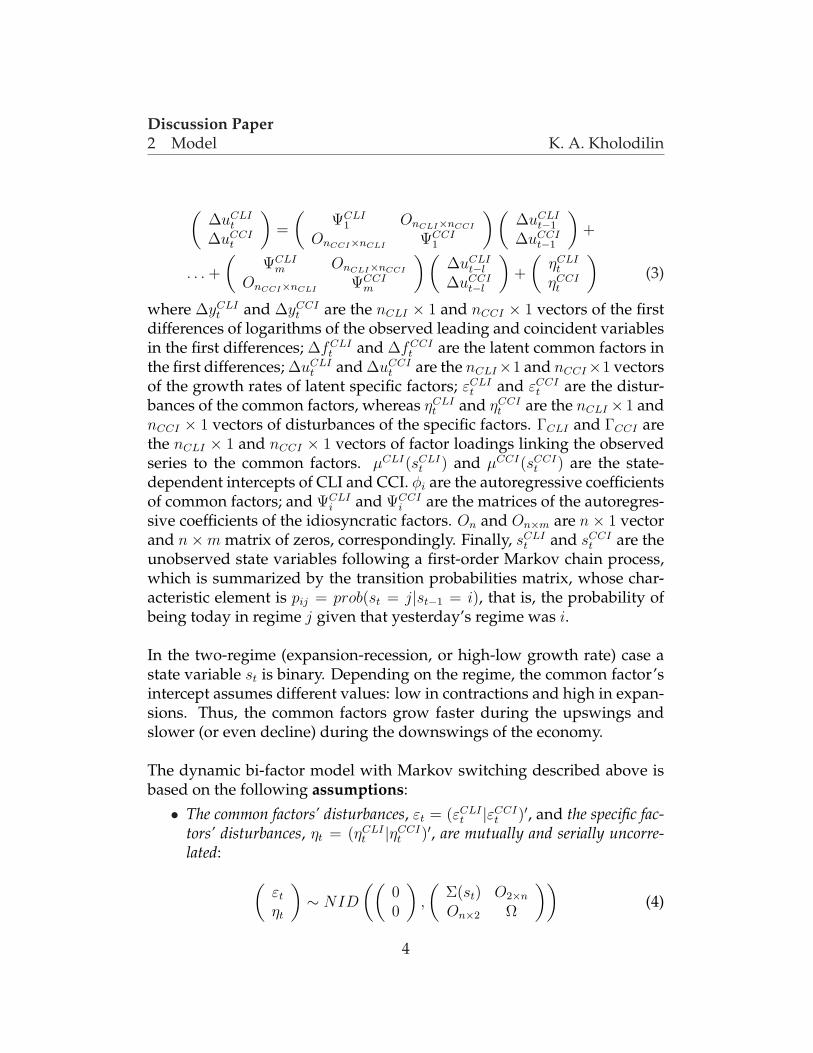
)(3)
where ∆yCLIt and ∆yCCI
t are the nCLI × 1 and nCCI × 1 vectors of the firstdifferences of logarithms of the observed leading and coincident variablesin the first differences; ∆fCLI
t and ∆fCCIt are the latent common factors in
the first differences; ∆uCLIt and ∆uCCI
t are the nCLI×1 and nCCI×1 vectorsof the growth rates of latent specific factors; εCLI
t and εCCIt are the distur-
bances of the common factors, whereas ηCLIt and ηCCI
t are the nCLI × 1 andnCCI × 1 vectors of disturbances of the specific factors. ΓCLI and ΓCCI arethe nCLI × 1 and nCCI × 1 vectors of factor loadings linking the observedseries to the common factors. µCLI(sCLI
t ) and µCCI(sCCIt ) are the state-
dependent intercepts of CLI and CCI. φi are the autoregressive coefficientsof common factors; and ΨCLI
i and ΨCCIi are the matrices of the autoregres-
sive coefficients of the idiosyncratic factors. On and On×m are n× 1 vectorand n×m matrix of zeros, correspondingly. Finally, sCLI
t and sCCIt are the
unobserved state variables following a first-order Markov chain process,which is summarized by the transition probabilities matrix, whose char-acteristic element is pij = prob(st = j|st−1 = i), that is, the probability ofbeing today in regime j given that yesterday’s regime was i.
In the two-regime (expansion-recession, or high-low growth rate) case astate variable st is binary. Depending on the regime, the common factor’sintercept assumes different values: low in contractions and high in expan-sions. Thus, the common factors grow faster during the upswings andslower (or even decline) during the downswings of the economy.
The dynamic bi-factor model with Markov switching described above isbased on the following assumptions:
• The common factors’ disturbances, εt = (εCLIt |εCCI
t )′, and the specific fac-tors’ disturbances, ηt = (ηCLI
t |ηCCIt )′, are mutually and serially uncorre-
lated:
(εt
ηt
)∼ NID
((00
),
(Σ(st) O2×n
On×2 Ω
))(4)
4

Discussion Paper2 Model K. A. Kholodilin
where Σ(st) is the diagonal 2 × 2 variance-covariance matrix of commonfactors, with the common factor residual variances on the main diagonal,σ2
CLI(st) and σ2CCI(st), which may be state dependent; Ω is the diagonal
n× n variance-covariance matrix of the idiosyncratic disturbances.
• There is no Granger causality between the common factors: φi.12 = φi.21 =0 ∀i ∈ [1, l]. This restriction together with the previous assumptionimply that the only way the CLI is linked to the CCI is through theintercept, when the state variables of both common factors are inter-dependent. There can also exist a relationship between the volatil-ities of two common factors when their residual variances are statedependent and their state variables are related. In principle, this as-sumption can be relaxed without changing much the outcomes ofthe model. Here it is used only for the sake of parsimony.
• This assumption specifies the state variable dynamics. In fact, we canconsider three cases:
(a) there is a single state variable, st, such that sCLIt = sCCI
t , in otherwords, the non-linear dynamics of the common factors are iden-tical;
(b) sCLIt and sCCI
t are completely independent;(c) sCLI
t and sCCIt are neither identical as in (a) nor independent as
in (b) but interdependent.
Now let us consider in more detail the specification of the Markov switch-ing in the non-linear dynamic bi-factor model under inspection. In thecase (a) above there is only one state variable and it all boils down to thestandard two-regime Markov switching model as in Hamilton (1989). Thetransition probabilities matrix then looks like:
π =
(p11 1− p11
1− p22 p22
)(5)
In the cases (b) and (c) there are two state variables: one per each commonfactor. This means that each composite indicator has its own recessionsand expansions. Therefore to describe the whole process, a compoundstate variable, comprising both sCLI
t and sCCIt , should be constructed as it
is done in Phillips (1991). This compound variable will have four differentstates:
5

Discussion Paper2 Model K. A. Kholodilin
Composite state variable st = 1 st = 2 st = 3 st = 4
Leading state variable sCLIt = 1 sCLI
t = 2 sCLIt = 1 sCLI
t = 2↑ ↓ ↑ ↓
Coincident state variable sCCIt = 1 sCCI
t = 1 sCCIt = 2 sCCI
t = 2↑ ↑ ↓ ↓
where the arrows show whether the economy goes up (expansion) or down(recession).
The dimension of the transition probabilities matrix is then 4 × 4 and itsstructure depends on which of the cases is assumed: (b) or (c). In thecase (b), when both state variables are independent, the transition prob-abilities matrix of the compound state variable is a Kronecker productof the transition probabilities matrices of the individual state variables:π = πCLI ⊗ πCCI . This is equivalent to:
π =
0BB@ pCLI11 pCCI
11 pCLI11 (1− pCCI
11 ) (1− pCLI11 )pCCI
11 (1− pCLI11 )(1− pCCI
11 )pCLI11 (1− pCCI
22 ) pCLI11 pCCI
22 (1− pCLI11 )(1− pCCI
22 ) (1− pCLI11 )pCCI
22(1− pCLI
22 )pCCI11 (1− pCLI
22 )(1− pCCI11 ) pCLI
22 pCCI11 pCLI
22 (1− pCCI11 )
(1− pCLI22 )(1− pCCI
22 ) (1− pCLI22 )pCCI
22 pCLI22 (1− pCCI
22 ) pCLI22 pCCI
22
1CCA(6)
Under the hypothesis (c) the two individual state variables are assumedto be interrelated in the sense that the CLI is supposed to enter the re-cessions (expansions) several periods earlier than the CCI. This is a kindof intermediate case between completely independent and identical statevariables corresponding to CLI and CCI.
As Phillips (1991) remarks, the model with an integer lag exceeding oneperiod would require a Markov process with the order higher than 1.However, the real-valued (positive) lag can be modelled with a first-orderMarkov process by constructing the following transition probabilities ma-trix:
π =
p11 1− p11 0 00 1− 1
A 0 1A
1B 0 1− 1
B 00 0 1− p22 p22
(7)
where A and B are the expected leads in the recession and expansion, cor-respondingly. For example, the expected lead of CLI with respect to CCI
6

Discussion Paper3 Data and Estimation K. A. Kholodilin
when entering the low-growth regime (st = 2) is obtained as:
A = p(st = 4|st−1 = 2) + 2p(st = 4|st−1 = 2)p(st = 2|st−1 = 2) + 3p(st = 4|st−1 = 2)p(st = 2|st−1 = 2)2 + . . .A = (1− p(st = 2|st−1 = 2)) + 2(1− p(st = 2|st−1 = 2))p(st = 2|st−1 = 2) + 3(1− p(st = 2|st−1 = 2))p(st = 2|st−1 = 2)2 + . . .A = (1− p(st = 2|st−1 = 2))
P∞k=0 kp(st = 2|st−1 = 2)k−1
A = (1− p(st = 2|st−1 = 2)) 11−p(st=2|st−1=2)2
A = 11−p(st=2|st−1=2)
(8)
We are going to examine three models corresponding to the three abovestated cases. By comparing these models one can test the underlying hy-potheses. Model (c) is an unrestricted version of model (a). Thus, by im-posing restrictions on the parameters A and B one can test the hypothesisof identical versus interdependent with lead non-linear cyclical dynam-ics, for example, using the Likelihood-ratio test. The null of identical statevariable implies that A = B = 1. The formal testing of (a) versus (b) or(c) versus (b) is a more complicated enterprise. Under the null of identicalor interdependent state variable the second state variable is not identified.It means that we are confronting the famous nuisance parameter problemsimilar, for instance, to testing the hypothesis of two regimes versus threeregimes.
In order to estimate the above dynamic factor models with Markov switch-ing, the linear part of the model is cast into the state-space form usingthe Kalman filter, whereas the Markov-switching part of the model is ex-pressed using the Hamilton filter. The estimations are carried out with themaximum likelihood method.
3 Data and Estimation
The component series of both CLI and CCI for the three large Europeaneconomies were taken from the various official publicly available sourceslike the data bases of central banks and statistical offices. The selection ofthe component series was based entirely on the empirical criteria. No eco-nomic theory has guided our choice. The following selection procedurewas employed.
The first step was to determine the leading and coincident time series. Theleading series are those with peaks and troughs occurring earlier than
7

Discussion Paper3 Data and Estimation K. A. Kholodilin
the peaks and troughs of some reference series. Therefore their cross-correlation with the reference series is highest when they are shifted back-wards. The coincident series have peaks and troughs coinciding withthose of the reference series. Hence their cross-correlation with the ref-erence series achieves its maximum at zero lag. As reference coincidentseries the index of industrial production was used. In many studies it istreated as a monthly proxy for the GDP, despite the fact that in the moderneconomy it accounts for less than a half of the whole output.
The second step has to do with the requirement that the components of acomposite indicator should be high enough but not too much correlatedamong themselves. It is important to avoid collinearity of the components.Therefore a kind of cluster analysis is needed to identify the groups of in-dicators with common dynamics.
The technique applied here is alike to the tree clustering, or joining1. As adistance measure the absolute value of contemporaneous cross-correlationis used. Shortly the algorithm runs as follows. For the whole data seta cross-correlation matrix is computed. Then a pair of variables havingthe highest absolute value of correlation is searched and united in a singlegroup. Graphically it means that they are drawn as two subbranches ofone branch. From these two variables a new variable is constructed as asimple mean. All the variables are initially standardized and hence haveequal unit variances. The new variable replaces the old ones in the dataset. For this new data set the correlation matrix is again estimated. Thecycle repeats until all there remains only one variable in the data set, thatis, the average of all the time series.
An example of such a tree can be seen on Figure 1. Three major groupsof indicators are easily distinguishable there. The first group includes thefinancial indicators (stock exchange index FTSE100, interest rates AJRP,AJLX and Spread, currency exchange rates AUSS and THAP) as well as thereal economy indicators (industrial production CKYW, number of prop-erty transactions FTAQ, and total passenger car production FFAO). Thesecond group includes mostly the business survey indicators (various Eu-ropean commission economic sentiment indicators BS-CONS, BS-INDU,
1For more details on cluster analysis see Everitt et al. (2001).
8

Discussion Paper3 Data and Estimation K. A. Kholodilin
BS-UK-ESI, and so on, CBI industrial trends survey ETCU and ETDQ,retail sales index EAPS, and average earnings index LNMQ). The thirdgroup consist of a mix of money market indicators (money stock M4 AUYN)and labor market indicators (employment in manufacturing YEJA, totalunemployment rate MGSX) and two other series.
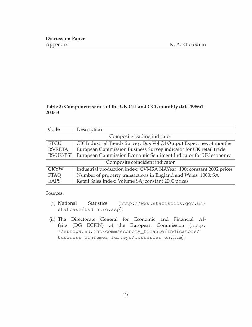
Combining both the leading-coincident analysis and clustering we haveidentified the components of the CLI and CCI. The former are mainly thebusiness survey indicators, whereas the latter are the real sector indicatorslike industrial production and retail trade. The complete list of componentseries for the UK see in Table 3.
The component series employed in this study are listed and shortly de-scribed in Tables 1 through 3 of Appendix.
All the series are tested for unit roots using the augmented Dickey-Fullertest. Each series is tested for random walk with drift and deterministictrend, random walk with drift, and random walk only. It turns out thatall the series have unit root. All the series are also tested for cointegration.The cointegration between the leading as well as between the coincidentseries was detected. As in Stock and Watson (1991) and Kim and Nelson(1999), the first differences of the logarithms of the original time series aretaken and then demeaned and standardized.
For each country we estimated two separate dynamic single-factor mod-els for CLI and CCI (with linear and Markov-switching dynamics) cor-responding to the hypotheses (b) and a dynamic bi-factor model withMarkov-switching corresponding to the hypothesis (c) presented in theprevious section. Recall that these hypotheses are defined by the follow-ing equations:
(a) Hypothesis of identical Markov-switching dynamics of CLI and CCI— equations (1) – (4) and (5). The model, in which CLI and CCI enterthe recessions and expansions simultaneously, without any leads.
(b) Hypothesis of independent Markov-switching dynamics of CLI andCCI — equations (1) – (4) and (6). This model can be alternativelyestimated as two separate dynamic single-factor models with two-regime switching based on coincident and leading indicators corre-
9

Discussion Paper3 Data and Estimation K. A. Kholodilin
spondingly. Each of the separate dynamic single-factor models isidentical to that of Chauvet (1998) and Kim and Nelson (1998).
(c) Hypothesis of interdependent Markov-switching dynamics of CLIand CCI — equations (1) – (4) and (7). A dynamic bi-factor modelwith interdependent cyclical dynamics that results in four-regimeswitching: two regimes for the leading indicator and two regimesfor the coincident indicator. The composite leading factor (or CLI)switches between its regimes earlier than the composite coincidentindicator (or CCI).
We determined the lag structure by balancing two requirements: on theone hand, our composite indicators should have some dynamics, that is,the lag order must be higher than zero; on the other hand, due to theshort sample the lag order cannot be too high. Therefore both the com-mon and idiosyncratic factors are specified as AR(1). For the identificationpurposes, the first loading factor in all the models is normalized to 1.
The parameter estimates and their standard errors corresponding to single-factor models of CLI and CCI and to bi-factor models are reported in Ta-bles 4 through 6. Both MS models of composite leading and coincidentindicators clearly distinguish between two regimes of positive and nega-tive growth rates.
The estimates of the non-switching parameters of the linear and Markov-switching models do not differ very much.
In the French and German case ∆CLI has a high positive autoregressivecoefficient varying for different models in the interval between 0.693 and0.823 for France and between 0.462 and 0.752 for Germany, whereas ∆CCIhas a negative, not always significant autoregressive coefficient varyingbetween -0.467 and -0.358 for France and between -0.228 and -0.131 forGermany. Correspondingly, as one can see on Figures 5 and 9, whichcompare the levels2 of the French and German composite indicators es-timated from the single- and bi-factor models, the CLI’s profile is muchsmoother than that of CCI. In the case of UK autoregressive coefficients of
2The levels of CLI and CCI are constructed as cumulated sums of their estimated firstdifferences. For example, CLIt = CLIt−1 + ∆CLIt.
10

Discussion Paper3 Data and Estimation K. A. Kholodilin
both ∆CLI and ∆CCI are not significantly different from zero suggestingthat the common factors are not persistent. Hence, as can be seen on Fig-ure 13, the profiles of British CLI and CCI are not so smooth.
Factor loadings are positive and in most cases significant. The values ofthe factor loadings are as a rule close to one and their dispersion is not veryhigh which is an indirect indicator of the approximately equal weights ofthe components. Therefore no single component is overinfluencing anycomposite indicator.
Under the bi-factor model with Markov switching the expected lead timesof CLI over CCI in recessions and expansions, A and B, can be computed.For France the expected lead in recessions is about 4 months and expectedlead in expansions is 1 month, for Germany both these leads are roughlyequal to 3 months, whereas for the UK the lead in recessions is approxi-mately 1 month and lead in expansions is roughly 3 months.
For the French CLI estimated as a single-factor model with Markov switch-ing the transition probability of being today in expansion given that yes-terday was expansion, p11 = 0.879, is slightly lower than the transitionprobability of being today in recession given that yesterday was recession,p22 = 1 − p12 = 0.898, implying that the expected duration of expansionsis approximately equal to 8 months and is lower than the expected dura-tion of recessions, which is about 10 months. For Germany the expecteddurations of expansions and recessions of CLI are 12 and 4 months andfor the UK these are 10 and 5 months respectively. The expected durationof the recessions of German and British CLIs are thus a bit too short. Theestimates of the dynamic single-factor model with Markov switching forCCI (see Tables 4–6) imply that the expected duration of the expansions ofFrench CCI is about 31 months and that of recessions is 15 months. Theexpected duration of the expansions and recessions of German CCI are 53months and 8 months correspondingly, whereas the expected durationsof expansions and recessions of the British CCI are 59 and 20 months re-spectively. Finally, according to the dynamic bi-factor model with Markovswitching that corresponds to the hypothesis (c), the expected durationsof expansions and recessions for France are 11 months both; the expectedduration of expansions of German cycle is 17 months and the expectedduration of recessions is about 4 months, while the expected durations of
11

Discussion Paper4 In-Sample Evaluation K. A. Kholodilin
expansions and recessions for the UK are 13 and 10 months respectively.
We can also test which of the two hypotheses, (a) or (c), fits the databest. For these two models the comparison the likelihood ratio test canbe accomplished. The critical value of the test statistic with two degreesof freedom and significance level of 1% is equal to LR0.01(2) = 9.21, at5% it is LR0.05(2) = 5.99, and at 10% it is LR0.10(2) = 4.61. For Francethe test statistic is LR = 2 × (LRc − LRa) = 2 × (−1592.6 + 1594.6) = 4,for Germany it is LR = 2 × (−1592.6 + 1594.6) = 37.4, and for UK it isLR = 2 × (−1817.7 + 1820.2) = 5. Therefore the null hypothesis of equalgoodness of fit of models (a) and (c) is rejected for Germany and UK andaccepted for France, implying that in case of Germany and UK the modelwith identical Markov-switching dynamics fits data worse than the modelwith the CLI leading the CCI.
4 In-Sample Evaluation
Unlike for the USA, we do not have any generally accepted business cyclechronology for France, Germany, and UK. Among the few available alter-native chronologies we chose two, to which the recession probabilities ofour non-linear models will be compared, namely the reference cycle datesdetermined and published by the Organization for Economic Cooperationand Development (OECD) and by the Economic Cycle Research Institute(ECRI). The OECD’s and ECRI’s chronologies for the three countries arereported in Table 7.
The third chronology we use here is based on the quarterly version of theBry-Boschan dating technique, which was suggested in ?. This chronol-ogy is obtained for the quarterly GDP data and is represented in the lasttwo columns of Table 7. For the analysis of the forecasting accuracy thequarterly dating is transformed into the monthly one: if in the quarterlychronology a quarter is recessionary (expansionary) then in the monthlychronology all the months belonging to this quarter are treated as reces-sionary (expansionary).
All these chronologies are plotted against the levels and year-on-year ratesof the real GDP in Figures 2–4. The BBQ chronology is supposed to reflect
12

Discussion Paper4 In-Sample Evaluation K. A. Kholodilin
the classical business cycle and hence it is compared to the level of theGDP. The other two chronologies are more likely to describe the growthcycle and therefore they are superimposed on the annual growth rates, orfourth-order differences of logs of the GDP.
Over the last 15 years the OECD detects five recessions for France, fourrecessions for Germany, and three recessions for the UK. At the same timeECRI finds three recessions for France, four recessions for Germany, andfour recessions for the UK.
The profiles of the French, German, and British CLI and CCI estimatedfrom the dynamic single- and bi-factor models with and without Markovswitching are plotted in Figures 5–13. The upper panels show the profilesof the composite indicators estimated with linear models, whereas the bot-tom panels depict the profiles of the CLI and CCI obtained with dynamicbi-factor models with Markov switching. It can be seen that the CLI hasoften the peaks and troughs that precede those of the CCI. This is espe-cially true for Germany — see Figure 9.
The filtered and smoothed conditional probabilities of recessions corre-sponding to the Markov-switching dynamic factor models examined hereare plotted in Figures 6–8 for France, Figures 10–12 for Germany, and Fig-ures 14–16 for the United Kingdom. The top panels show the conditionalrecession probabilities for the dynamic single-factor models, whereas theconditional recession probabilities derived from the dynamic bi-factor modelare shown on the bottom panel of each figure. The bold continuous linescorrespond to the low-state probabilities of CLI, while the dashed lines tothose of CCI. The shaded areas represent the recessionary phases of thecorresponding reference chronology. In the bi-factor models with interde-pendent Markov-switching dynamics (two state variables), there are fourregimes: two for the CLI and two for the CCI. The recession probabili-ties of the CLI are computed as the sum of the conditional probabilities ofregimes 2 and 4 (”low leading factor and high coincident factor” and ”lowleading factor and low coincident factor”), while CCI’s recession proba-bilities are the sum of the probabilities of regimes 3 and 4. The recessionprobabilities stemming from the two models — (b) and (c) — are very dif-ferent.
13

Discussion Paper4 In-Sample Evaluation K. A. Kholodilin
Under the hypothesis of the independent cycles of CLI and CCI (model(b)), the conditional recession probabilities of CLI are quite volatile evenafter smoothing — see the upper panels of Figures 6–14. For France — Fig-ure 6 — the CLI’s recession probabilities signal six recessions (two of themin 2001–2002 are so close to each other that can be merged into a singlerecession). All of them fall into the shaded regions, the second, third, andfourth model-derived recessions significantly lead the OECD’s recessions.French CCI has only two recessions: one in the beginning of sample andanother, longer one, in the end of it. They seem to start and end in accor-dance with the chronology of the OECD. For Germany — Figure 10 — fivemodel-derived recessions of CLI can be observed. All of them belong tothe shaded areas of the OECD’s dating. The CCI’s conditional recessionprobabilities give only two signals of downswings: in 1992 and in 2001.The second signal is rather weak being lower than 0.5. For UK — Fig-ure 14 — the dynamic single-factor model of CLI detects two recessionscoinciding with the first two recessions of OECD and three rather short-lived recessions in the end of the sample that fall into the shaded area. Themodel of British CCI allows detecting only two recessions: one long in thebeginning and another shorter in the end of the sample. Both lag behindthe model-derived recessions of CLI.
The picture changes substantially when model (c) is considered. The cor-responding conditional recession probabilities can be seen on the bottompanels of Figures 6–14. In the case of France the probabilities of the lowstate of CLI became smoother, whereas those of CCI have undergone sig-nificant changes: there are six model-derived recession of CCI now thatbegin and finish later than the recession probabilities of CLI. One can seethat the delay is longer at the beginning of recessions and shorter at the be-ginning of expansions, which perfectly accords with the values of the pa-rameters A and B reported in Table 4 and discussed above. In the case ofGermany the conditional recession probabilities of CLI underwent ratherminor change. By contrast, the recession probabilities of CCI started re-sembling those of CLI with a clearly visible lag. Now both CLI and CCIsignal five recessions. In the case of UK both the recession probabilitiesof CLI and CCI have been modified. The former now have eight peaksexceeding 0.5 margin but only six of them remain above 0.5 for a longenough time. The conditional recession probabilities of CCI under model(c) resemble those of CLI with a little lag, which is bigger when the shifts
14

Discussion Paper4 In-Sample Evaluation K. A. Kholodilin
from low- to high-state take place.
When the predicted reference chronology is known, the above comparisonof the in-sample forecasting performance can be formalized using somecriterion that measures the difference between the reference chronologyand the model-derived dating. For this purpose we use the QuadraticProbability Score (QPS) proposed in Brier (1950), which is based on prob-abilities derived from each model. Let Pt be the conditional probabilitythat the economy is in recession, estimated from the model; let Rt be abinary reference chronology (1 if recession, 0 otherwise), and the slightlymodified version of QPS is given by:
QPS =1
T− | τ |T−0.5(|τ |−τ)∑
t=0.5(|τ |+τ)+1
(Pt−τ −Rt)2 (9)
where τ is the integer denoting the time shift that accounts for the possi-bly leading (τ > 0), coincident (τ = 0) or lagging (τ < 0) character of therecession probabilities and Pt. QPS varies between 0 and 1, with a scoreof 0 corresponding to perfect accuracy. This is the unique proper scoringrule that is only a function of the discrepancy between realizations andmodel-derived probabilities (see Diebold and Rudebusch (1989) for fur-ther discussion).
The in-sample predicting performance of the non-linear models estimatedin this paper is compared to that of the Markov-Switching Vector Autore-gressions (MSVAR) with two regimes estimated using the Ox package ofH.-M.Krolzig3 and is reported in Tables 8–10. The MSVARs include thecomponent series of the dynamic bi-factor models: the ”CLI” means thatthe components of CLI are employed, ”CCI” — the components of CCI,and ”All” — that both the components of CLI and CCI are used. Fivetypes of the MSVAR model are considered: Markov switching with state-dependent intercept (MSI), Markov switching with state-dependent inter-cept and variance (MSIH), Markov switching with state-dependent mean(MSM), Markov switching with state-dependent intercept and autoregres-sive parameters (MSIA), and Markov switching with state-dependent in-tercept, variance, and autoregressive parameters (MSIAH).
3More details on the types of MSVAR models see in ?.
15
Discussion Paper4 In-Sample Evaluation K. A. Kholodilin
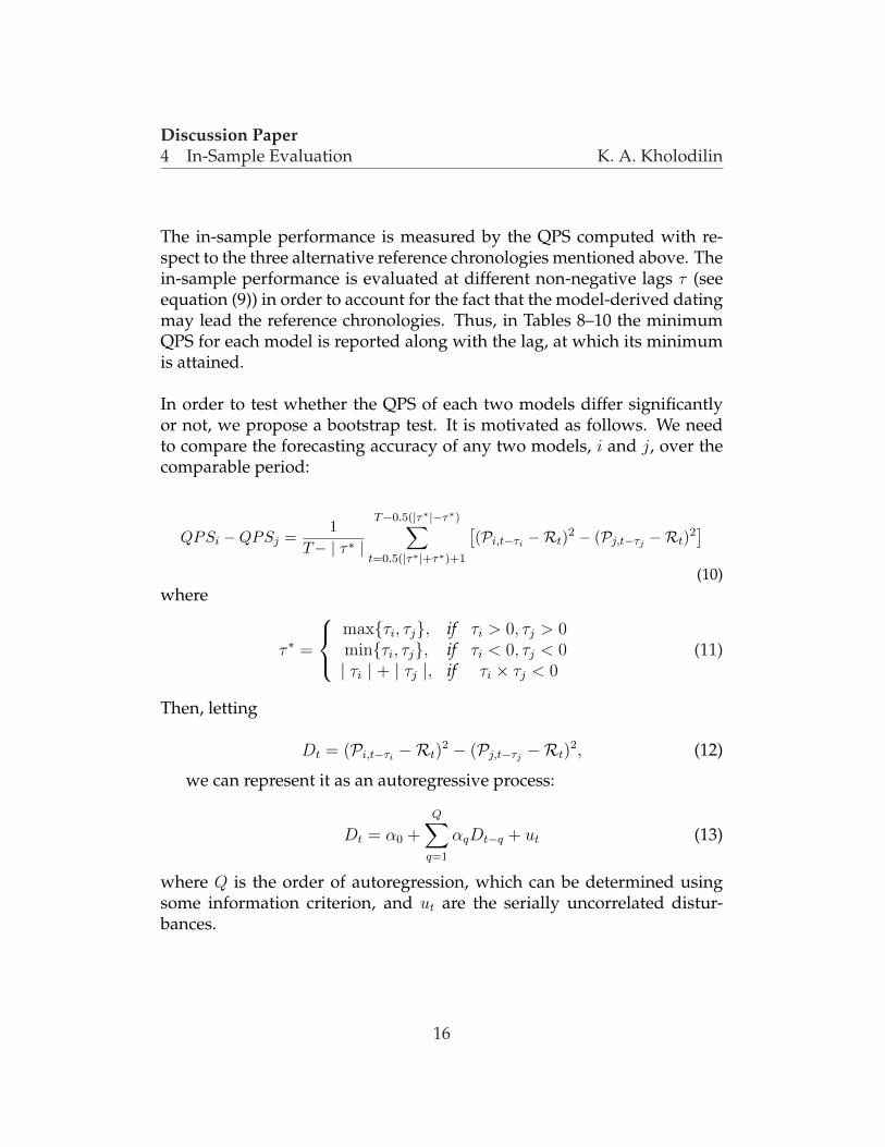
The in-sample performance is measured by the QPS computed with re-spect to the three alternative reference chronologies mentioned above. Thein-sample performance is evaluated at different non-negative lags τ (seeequation (9)) in order to account for the fact that the model-derived datingmay lead the reference chronologies. Thus, in Tables 8–10 the minimumQPS for each model is reported along with the lag, at which its minimumis attained.
In order to test whether the QPS of each two models differ significantlyor not, we propose a bootstrap test. It is motivated as follows. We needto compare the forecasting accuracy of any two models, i and j, over thecomparable period:
QPSi −QPSj =1
T− | τ∗ |T−0.5(|τ∗|−τ∗)∑
t=0.5(|τ∗|+τ∗)+1
[(Pi,t−τi −Rt)2 − (Pj,t−τj −Rt)2
]
(10)where
τ ∗ =
maxτi, τj, if τi > 0, τj > 0minτi, τj, if τi < 0, τj < 0| τi | + | τj |, if τi × τj < 0
(11)
Then, letting
Dt = (Pi,t−τi−Rt)
2 − (Pj,t−τj−Rt)
2, (12)
we can represent it as an autoregressive process:
Dt = α0 +
Q∑q=1
αqDt−q + ut (13)
where Q is the order of autoregression, which can be determined usingsome information criterion, and ut are the serially uncorrelated distur-bances.
16

Discussion Paper4 In-Sample Evaluation K. A. Kholodilin
Hence testing the null hypothesis of statistically equal forecasting accu-racy of model i and model j, that is, QPSi = QPSj , is equivalent to test-ing the null of α0 = 0. However, we do not know the distribution of Dt
and cannot be sure that the standard Student distribution is applicable.Therefore we obtain the distribution through the bootstrap. This is doneas follows:
(1) Estimate equation (13) and save the estimated parameters, α′ = α0, . . . , αQ,and the vector of errors, u′ = u0.5(|τ∗|+τ∗)+1, . . . , uT−0.5(|τ∗|−τ∗).
(2) Generate a bootstrap sample of size T− | τ ∗ | using the vector of esti-mated parameters α and the pseudo-disturbances drawn with replace-ment from the vector of errors u:
Drt = α0 +
Q∑q=1
αqDrt−q + ur
t (14)
where r denotes the r-th bootstrap replication.
(3) Compute the estimates of α from the sample and save αr0.
(4) Repeat steps (2)–(3) R times (R should be sufficiently large that its fur-ther increases have no important effect on results) and find the boot-strap p-values as: if 1
R
∑Rr=1 αr
0 > 0, then compute the proportion of αr0
that are lower than 0; otherwise compute the proportion of αr0 that are
greater than 0. If the proportion is higher than some chosen signifi-cance level, say 0.05, then the null of no difference between two QPSsis accepted, otherwise it is rejected.
We do not reproduce the p-values here because the corresponding tableswould occupy too much space. However, we will heavily rely on themwhen discussing the results below. The number of bootstrap replicationswas R = 2000.
On average, for all the countries the in-sample forecasting performanceof most of the models is not very satisfactory, since QPS is relatively high.In addition, most datings derived from the models based either on thesubset of the leading indicators or on the whole set of data conform much
17

Discussion Paper4 In-Sample Evaluation K. A. Kholodilin
better with the OECD’s and ECRI’s chronologies than with that of BBQ.By contrast, the models including the coincident component series onlyare better forecasting the BBQ chronology. Thus, it appears that the lead-ing series better reflect the growth cycles, whereas the coincident variablesare less volatile and hence are proxies for the classical cycle.
For France, as Table 8 shows, the OECD is best predicted by the follow-ing three models: bi-factor model (a), the CLI in the bi-factor model (c)and the CLI in the bi-factor model (b). Recall that the LR-test gave pref-erence to the model (a) over the model (c). The lowest QPS are achievedat leads equal to 2–6 months. The MSVAR models, for which the null ofno difference in the forecasting accuracy could not be rejected, are: themodels MSI and MSM of the components of CLI, MSM-CCI and severalmodels including all the component series. The same picture is for thechronology of the ECRI, although the lead time is very small, varying from0 to 2 months. Once more the closest rivals, for which the null cannot berejected, are MSI-CLI, MSM-CLI, MSIAH-CLI, MSM-CCI, MSIA-All andMSIAH-All. However, the MSVAR models attain the minimum of QPSat the negative lags, which means that they are lagging behind the ECRI’sgrowth cycle, whereas our objective is to find the models that forecast welland are leading. The three models having the highest conformity with theBBQ-chronology, however, are different. These are: single-factor model ofCCI, MSIH and MSM models for the components of CCI. The in-sampleperformance of the first two models is not statistically different, but bothof them significantly outperform MSM-CCI and all the other models.
The models that best of all detect the turning points of the OECD’s chronol-ogy for Germany are: MSI, MSM, and MSIAH including all the componentseries. The corresponding model-derived probabilities lead the OECD’scycle by 1–2 months. The best performance among the dynamic factormodels has model (c). Despite the fact that the QPS of the latter are higherthan those of the best MSVAR models, there is no statistically significantdifference between their forecasting accuracy. The best conformity withGerman ECRI’s dating is displayed by MSI model based on the compo-nents of CCI as well as by the MSM and MSIA models including the com-ponents of CLI. Only MSIA model is leading the reference chronology by2–5 months, the other model-derived chronologies coincide with the ref-erence one, save the filtered recession probabilities of MSM that are even
18

Discussion Paper5 Summary K. A. Kholodilin
lagging behind the ECRI’s growth cycle. Again, according to our empir-ical p-values the difference between these models and dynamic bi-factormodel (c) is not significant. The three models that are best at in-sampleprediction of the turns of German classical cycle are: bi-factor model (c),bi-factor model (b), and bi-factor model (a). These do not differ (at 5%significance level) in accuracy from the MSVAR models based on the com-ponents of CCI.
Finally, the OECD’s chronology for UK is best predicted within the sampleby the dynamic bi-factor model (c) with lead equal to 1–3 months, MSIAmodel for the components of CCI (lead time is 1 month), and MSIH modelfor the components of CLI (lead time is 8 months). The hypothesis of theequal forecasting accuracy of these models cannot be rejected at 5% signif-icance level. The three models having the highest conformity with ECRI’sgrowth cycle are: dynamic bi-factor model (c) with lag up to 5 months,MSIA-CLI model with lag of 1 month, and MSM-CLI model with lag of 1month for the filtered probabilities and lead of 2 months for the smoothedones. These three models have equal in-sample performance. The clas-sical cycle represented by the BBQ chronology is best of all detected bythe dynamic single-factor model of CCI (that is, dynamic bi-factor model(b)) with lag of 2 months for filtered probabilities and lag of 6 monthsfor smoothed ones, MSM-CCI and MSI-CCI models with the same lags.These models have statistically equal forecasting performance but are sig-nificantly different from most other models, save those MSVAR modelsthat are based on the components of CCI.
Given the uncertainty about the reference chronology, the out-of-sampleforecasting exercise is hardly possible. Of course, we can make the fore-casts with our models but their eventual performance will be affected bothby the forecasting errors and by the fact that it is not sure whether the se-lected reference chronologies reflect well the turning points of the businesscycle in the three European countries under inspection.
5 Summary
In this paper a dynamic factor model with Markov-switching and twocommon factors, one of which is leading and another coincident, is esti-
19

Discussion PaperReferences K. A. Kholodilin
mated for the three large European economies: France, Germany, and UK.The separation of the data set into the group of leading and the group ofcoincident indicators and estimation of one common factor per each groupallows more efficient use of the available information. The predictive con-tent of CLI permits detecting the turns of CCI in advance. As a rule theleading indicators composing the CLI are more readily available and sub-ject to less important revisions than the coincident indicators.
Three alternative hypotheses concerning the temporal relationship betweenthe CLI and CCI were examined: (a) switches between the recessionaryand expansionary phases of CLI and CCI are identical; (b) these switcheshappen independently; and (c) the switches of the CLI precede those ofCCI with some positive lead. In the latter case one of the outputs of themodel are the estimates of the expected lead time of CLI over CCI bothat peaks and troughs. The largest expected lead equal to 4 months wasfound for France and the smallest expected lead of 1 month, which vir-tually means that both composite indicators enter the same cyclical phasesimultaneously, for the UK.
The test of in-sample performance of models examined in the paper isconducted relative to the turning points of the three reference chronolo-gies: those of OECD and ECRI that reflect the growth cycle concept andthat of BBQ describing the classical cycle. The measure of conformity be-tween the model-derived and reference cycles is the QPS. In addition, thethe performance of the MSVAR models is computed. It appears that theranking is highly dependent on the reference chronology. For France it isour dynamic bi-factor models that capture the turns of the growth cyclesthe best. For Germany the some MSVAR models perform better, whereasfor the UK the first positions in the performance ranking are shared bothby bi-factor and certain MSVAR models.
References
Bandholz, H. (2005). New composite leading indicators for Hungary andPoland. Ifo Working Paper No. 3.
Bandholz, H. and M. Funke (2003). In search of leading indicators of eco-
20

Discussion PaperReferences K. A. Kholodilin
nomic activity in Germany. Journal of Forecasting 22, 277–297.
Brier, G. (1950). Verification of forecasts expressed in terms of probability.Monthly Weather Review 78, 1–3.
Burns, A. and W. Mitchell (1946). Measuring Business Cycles. New York.
Chauvet, M. (1998). An econometric characterization of business cycledynamics with factor structure and regime switching. International Eco-nomic Review 39, 969–996.
Chauvet, M. (2002). The Brazilian business and growth cycles. RevistaBrasileira de Economia 56(1).
Diebold, F. X. and G. D. Rudebusch (1989). Scoring the leading indicators.Journal of Business 62, 369–402.
Diebold, F. X. and G. D. Rudebusch (1996). Measuring business cycles: Amodern perspective. The Review of Economics and Statistics 78, 67–77.
Everitt, B. S., S. Landau, and M. Leese (2001). Cluster Analysis. OxfordUniversity Press.
Hamilton, J. D. (1989). A new approach to the economic analysis of nonsta-tionary time series and the business cycle. Econometrica 57(2), 357–384.
Kaufmann, S. (2000). Measuring business cycles with a dynamic Markovswitching factor model: An assessment using Bayesian simulationmethods. Econometrics Journal 3, 39–65.
Kholodilin, K. A. (2001). Latent leading and coincident factors model withMarkov-switching dynamics. Economics Bulletin 3(7), 1–13.
Kholodilin, K. A. (2002). Two alternative approaches to modelling the non-linear dynamics of the composite economic indicator. Economics Bul-letin 3(26), 1–18.
Kholodilin, K. A. and V. W. Yao (2005). Measuring and predicting turningpoints using a dynamic bi-factor model. International Journal of Forecast-ing 21, 525–537.
21

Discussion PaperReferences K. A. Kholodilin
Kim, C.-J. (1994)). Dynamic linear models with Markov-switching. Journalof Econometrics 60, 1–22.
Kim, C.-J. and C. R. Nelson (1998). Business cycle turning points, a newcoincident index, and tests of duration dependence based on a dynamicfactor model with regime switching. The Review of Economics and Statis-tics 80(2), 188–201.
Kim, C.-J. and C. R. Nelson (1999). State-Space Models with Regime Switch-ing: Classical and Gibbs-Sampling Approaches with Applications. Cam-bridge: MIT Press.
Kim, M.-J. and J.-S. Yoo (1995). New index of coincident indicators: A mul-tivariate Markov switching factor model approach. Journal of MonetaryEconomics 36, 607–630.
Phillips, K. L. (1991). A two-country model of stochastic output withchanges in regime. Journal of International Economics 31, 121–142.
Stock, J. H. and M. W. Watson (1991). A probability model of the coinci-dent economic indicators. In L. K. and M. G. (Eds.), Leading EconomicIndicators: New Approaches and Forecasting Records. Cambridge Univer-sity Press.
Watanabe, T. (2003, February). Measuring business cycle turning pointsin Japan with a dynamic Markov switching factor model. Monetary andEconomic Studies 21(1).
22

Discussion PaperAppendix K. A. Kholodilin
Appendix
Table 1: Component series of the French CLI and CCI, monthly data1992:1–2005:4
Code DescriptionComposite leading indicator
EC-NivCC Niveau du carnet de commandesEC-StockPFPrevu Stocks de produits finis prevus pour les prochains moisTHE THE — Taux de rendement des emprunts d’etat LT FMCAC40 Bourse Paris CAC 40 (adj. close)
Composite coincident indicatorIPI Index de la production industrielleip-agric Index de la production — Industries agricoles et alimentairesexport-ocde Exportations FAB; Valeur brute; OCDE; euroimport-ocde Importation CAF; Valeur brute; OCDE; euro
Sources:
(i) Banque de France (http://www.banque-france.fr/fr/stat_conjoncture/series/series.htm) ;
(ii) INSEE (http://www.indices.insee.fr/bsweb/servlet/bsweb );
(iii) Yahoo! Finance (http://fr.finance.yahoo.com/q/hp?s=%5EFCHI).
23

Discussion PaperAppendix K. A. Kholodilin
Table 2: Component series of the German CLI and CCI, monthly data1991:1–2005:3
Code DescriptionComposite leading indicator
IFO Das Ifo Geschaftsklima fur die Gewerbliche Wirtschaft,Erwartungen (R3), 2000=100, SA)
SU0253 Geldmarktsatze am Frankfurter Bankplatz, Dreimonatsgeld,Monatsdurchschnitt
WU3141 DAX-Index, 1987 = 1000YU0516 HWWA-Rohstoffpreisindex ”Euroland”
Composite coincident indicatorUXNI63 Produktion IndustrieUXA001 Auftragseingang in Verarbeitendes Gewerbe, Werte,
arbeitstaglich bereinigtUXHK87 Einzelhandelumsatz, Volumen, kalenderbereinigtUUCC04 Offene Stellen InsgesamtEU2001 Außenhandel, Warenhandel, Ausfuhr (fob)
Source:Deutsche Bundesbank (http://www.bundesbank.de/statistik/statistik_zeitreihen.php ).
24
Discussion PaperAppendix K. A. Kholodilin
Table 3: Component series of the UK CLI and CCI, monthly data 1986:1–2005:3
Code DescriptionComposite leading indicator
ETCU CBI Industrial Trends Survey: Bus Vol Of Output Expec: next 4 monthsBS-RETA European Commission Business Survey indicator for UK retail tradeBS-UK-ESI European Commission Economic Sentiment Indicator for UK economy
Composite coincident indicatorCKYW Industrial production index: CVMSA NAYear=100; constant 2002 pricesFTAQ Number of property transactions in England and Wales: 1000; SAEAPS Retail Sales Index: Volume SA; constant 2000 prices
Sources:
(i) National Statistics (http://www.statistics.gov.uk/statbase/tsdintro.asp );
(ii) The Directorate General for Economic and Financial Af-fairs (DG ECFIN) of the European Commission (http://europa.eu.int/comm/economy_finance/indicators/business_consumer_surveys/bcsseries_en.htm ).
25

Discussion PaperAppendix K. A. Kholodilin
Tabl
e4:
Esti
mat
esof
the
para
met
ers
ofFr
ench
sing
le-
and
bi-f
acto
rli
near
and
Mar
kov-
swit
chin
gm
odel
s,m
onth
lyda
ta19
92:1
–200
5:4
Mod
el(a
)M
odel
(b):
Com
posi
teLe
adin
gIn
dica
tor
Mod
el(c
)Pa
ram
eter
LL=-
1594
.6Pa
ram
eter
Line
ar,L
L=-8
68.4
MS,
LL=-
866.
9Pa
ram
eter
LL=-
1592
.6C
oeff
St.e
rror
Coe
ffSt
.err
orC
oeff
St.e
rror
Coe
ffSt
.err
orp11
0.90
10.
041
p11
——
0.87
90.
069
p11
0.90
80.
043
p12
0.09
40.
044
p12
——
0.10
20.
057
p22
0.91
20.
042
µC
LI.1
0.43
80.
163
µC
LI.1
——
0.24
10.
072
A3.
740
2.87
0µ
CL
I.2
-0.4
400.
168
µC
LI.2
——
-0.2
150.
072
B1.
310
1.47
0µ
CC
I.1
0.34
90.
096
γS
tPF
Prevu
0.22
50.
093
0.19
10.
098
µC
LI.1
0.25
20.
083
µC
CI.2
-0.3
560.
095
γT
HE
0.39
40.
125
0.39
60.
127
µC
LI.2
-0.2
120.
068
γS
tPF
Prevu
0.21
50.
095
γC
AC
40
0.22
60.
132
0.23
60.
141
µC
CI.1
0.29
90.
103
γT
HE
0.36
20.
133
φC
LI
0.82
30.
071
0.71
20.
115
µC
CI.2
-0.3
450.
111
γC
AC
40
0.24
40.
128
ψN
ivC
C-0
.201
0.10
5-0
.181
0.10
2γ
StP
FP
revu
0.18
10.
097
γIP
I−
Agr
0.48
80.
111
ψS
tPF
Prevu
-0.3
350.
076
-0.3
290.
077
γT
HE
0.40
10.
129
γE
xp−
OC
DE
1.08
00.
101
ψT
HE
-0.0
650.
083
-0.0
590.
082
γC
AC
40
0.24
40.
14γ
Im
p−
OC
DE
1.09
00.
105
ψC
AC
40
0.00
80.
045
0.00
50.
107
γIP
I−
Agr
0.49
30.
114
φC
LI
0.31
00.
270
σC
LI
0.15
40.
060
0.03
60.
051
γE
xp−
OC
DE
1.08
00.
106
φC
CI
-0.4
660.
082
σN
ivC
C0.
497
0.08
60.
553
0.09
0γ
Im
p−
OC
DE
1.09
00.
111
ψN
ivC
C-0
.197
0.11
9σ
StP
FP
revu
0.86
20.
098
0.87
60.
099
φC
LI
0.69
30.
126
ψS
tPF
Prevu
-0.3
320.
077
σT
HE
0.91
60.
106
0.92
40.
106
φC
CI
-0.4
670.
078
ψT
HE
-0.0
650.
081
σC
AC
40
0.97
00.
110
0.97
00.
110
ψN
ivC
C-0
.186
0.09
9ψ
CA
C40
0.00
20.
066
Mod
el(b
):C
ompo
site
Coi
ncid
entI
ndic
ator
ψS
tPF
Prevu
-0.3
230.
076
ψIP
I-0
.400
0.09
3Pa
ram
eter
Line
ar,L
L=-7
37.8
MS,
LL=-
737.
0ψ
TH
E-0
.051
0.08
1ψ
IP
I−
Agr
-0.2
680.
081
Coe
ffSt
.err
orC
oeff
St.e
rror
ψC
AC
40
0.01
50.
065
ψE
xp−
OC
DE
-0.3
860.
097
p11
——
0.96
80.
044
ψIP
I-0
.413
0.09
0ψ
Im
p−
OC
DE
-0.4
090.
099
p12
——
0.06
70.
086
ψIP
I−
Agr
-0.2
590.
081
σC
LI
0.15
10.
156
µC
CI.1
——
0.13
00.
136
ψE
xp−
OC
DE
-0.3
860.
100
σC
CI
0.40
70.
078
µC
CI.2
——
-0.3
080.
255
ψIm
p−
OC
DE
-0.3
960.
098
σN
ivC
C0.
447
0.15
7γ
IP
I−
Agr
0.48
80.
109
0.48
80.
110
σC
LI
0.02
90.
047
σS
tPF
Prevu
0.86
40.
099
γE
xp−
OC
DE
1.06
00.
101
1.07
00.
101
σC
CI
0.39
70.
077
σT
HE
0.92
20.
106
γIm
p−
OC
DE
1.07
00.
105
1.08
00.
105
σN
ivC
C0.
563
0.09
5σ
CA
C40
0.96
20.
109
φC
CI
-0.3
580.
086
-0.4
010.
088
σS
tPF
Prevu
0.87
60.
100
σIP
I0.
306
0.04
8ψ
IP
I-0
.416
0.09
3-0
.410
0.09
3σ
TH
E0.
925
0.10
6σ
IP
I−
Agr
0.75
00.
086
ψIP
I−
Agr
-0.2
700.
081
-0.2
690.
081
σC
AC
40
0.96
90.
109
σE
xp−
OC
DE
0.24
70.
047
ψE
xp−
OC
DE
-0.3
670.
098
-0.3
710.
098
σIP
I0.
298
0.04
7σ
Im
p−
OC
DE
0.30
10.
052
ψIm
p−
OC
DE
-0.3
970.
100
-0.4
060.
100
σIP
I−
Agr
0.75
10.
087
σC
CI
0.53
20.
094
0.48
90.
092
σE
xp−
OC
DE
0.24
60.
048
σIP
I0.
296
0.04
80.
300
0.04
8σ
Im
p−
OC
DE
0.30
10.
053
σIP
I−
Agr
0.74
70.
086
0.74
80.
086
σE
xp−
OC
DE
0.25
40.
048
0.25
30.
048
σIm
p−
OC
DE
0.30
50.
053
0.30
10.
053
Not
e:LL
isth
elo
g-lik
elih
ood
func
tion
valu
e
26

Discussion PaperAppendix K. A. Kholodilin
Tabl
e5:
Esti
mat
esof
the
para
met
ers
ofG
erm
ansi
ngle
-an
dbi
-fac
tor
line
aran
dM
arko
v-sw
itch
ing
mod
els,
mon
thly
data
1991
:1–2
005:
3
Mod
el(a
)M
odel
(b):
Com
posi
teLe
adin
gIn
dica
tor
Mod
el(c
)Pa
ram
eter
LL=-
2011
.0Pa
ram
eter
Line
ar,L
L=-9
09.9
MS,
LL=-
907.
5Pa
ram
eter
LL=-
1992
.3C
oeff
St.e
rror
Coe
ffSt
.err
orC
oeff
St.e
rror
Coe
ffSt
.err
orp11
0.98
30.
023
p11
——
0.91
70.
070
p11
0.94
10.
026
p12
0.12
20.
100
p12
——
0.27
20.
170
p22
0.72
90.
114
µC
LI
10.
008
0.03
1µ
CL
I1
——
0.17
00.
066
A2.
870
1.35
0µ
CL
I2
-0.0
580.
130
µC
LI
2—
—-0
.554
0.24
3B
3.29
01.
870
µC
CI
10.
126
0.09
3γ
SU
0253
0.55
00.
266
0.69
80.
301
µC
LI
10.
153
0.05
2µ
CC
I2
-0.9
510.
339
γW
U3141
0.63
10.
228
0.86
50.
295
µC
LI
2-0
.483
0.14
2γ
SU
0253
0.50
20.
262
γY
U0516
0.58
00.
264
0.65
70.
286
µC
CI
10.
212
0.08
5γ
WU
3141
0.66
20.
236
φC
LI
0.75
20.
081
0.44
30.
319
µC
CI
2-0
.574
0.17
0γ
YU
0516
0.61
00.
271
ψIF
O0.
081
0.13
90.
179
0.11
8γ
SU
0253
0.81
50.
289
γU
XA
001
0.81
90.
208
ψS
U0253
0.37
50.
076
0.37
00.
077
γW
U3141
0.83
70.
212
γU
XH
K87
0.27
10.
121
ψW
U3141
-0.1
620.
090
-0.2
110.
085
γY
U0516
0.64
50.
252
γU
UC
C04
0.12
40.
115
ψY
U0516
0.29
40.
078
0.30
50.
077
γU
XA
001
0.80
20.
180
γE
U2001
0.48
70.
151
σC
LI
0.14
80.
079
0.01
80.
044
γU
XH
K87
0.23
50.
117
φC
LI
0.73
20.
092
σIF
O0.
648
0.12
70.
737
0.10
9γ
UU
CC
04
0.10
00.
099
φC
CI
-0.2
530.
142
σS
U0253
0.74
90.
088
0.74
70.
086
γE
U2001
0.50
80.
138
ψIF
O0.
100
0.12
5σ
WU
3141
0.83
70.
108
0.78
30.
101
φC
LI
0.46
20.
149
ψS
U0253
0.34
30.
076
σY
U0516
0.80
20.
095
0.81
40.
093
φC
CI
-0.2
280.
131
ψW
U3141
-0.1
670.
090
Mod
el(b
):C
ompo
site
Coi
ncid
entI
ndic
ator
ψIF
O0.
184
0.08
4ψ
YU
0516
0.29
60.
078
Para
met
erLi
near
,LL=
-107
5.8
MS,
LL=-
1071
.0ψ
SU
0253
0.35
10.
076
ψU
XN
I63
-0.3
610.
099
Coe
ffSt
.err
orC
oeff
St.e
rror
ψW
U3141
-0.1
980.
083
ψU
XA
001
-0.3
760.
086
p11
——
0.98
00.
024
ψY
U0516
0.30
10.
075
ψU
XH
K87
-0.3
830.
072
p12
——
0.12
30.
094
ψU
XN
I63
-0.3
590.
098
ψU
UC
C04
0.63
00.
063
µC
CI
1—
—0.
142
0.10
0ψ
UX
A001
-0.3
890.
082
ψE
U2001
-0.3
300.
076
µC
CI
2—
—-0
.923
0.30
2ψ
UX
HK
87
-0.3
850.
072
σC
LI
0.14
60.
077
γU
XA
001
0.57
50.
232
0.74
50.
196
ψU
UC
C04
0.66
40.
071
σC
CI
0.35
90.
140
γU
XH
K87
0.27
60.
108
0.28
80.
114
ψE
U2001
-0.3
730.
064
σIF
O0.
661
0.12
1γ
UU
CC
04
0.12
40.
100
0.16
70.
118
σC
LI
0.01
70.
032
σS
U0253
0.79
20.
092
γE
U2001
0.32
90.
117
0.39
00.
109
σC
CI
0.36
40.
112
σW
U3141
0.83
00.
108
φC
CI
-0.1
650.
155
-0.2
760.
141
σIF
O0.
747
0.09
2σ
YU
0516
0.79
60.
095
ψU
XN
I63
-0.3
830.
143
-0.3
680.
107
σS
U0253
0.73
60.
084
σU
XN
I63
0.44
70.
129
ψU
XA
001
-0.3
680.
083
-0.3
910.
086
σW
U3141
0.80
60.
097
σU
XA
001
0.60
00.
103
ψU
XH
K87
-0.3
890.
072
-0.3
870.
073
σY
U0516
0.81
80.
092
σU
XH
K87
0.81
00.
091
ψU
UC
C04
0.58
10.
066
0.58
00.
066
σU
XN
I63
0.43
80.
116
σU
UC
C04
0.60
50.
067
ψE
U2001
-0.5
230.
069
-0.5
310.
068
σU
XA
001
0.59
90.
096
σE
U2001
0.80
30.
094
σC
CI
0.67
50.
286
0.40
00.
159
σU
XH
K87
0.81
30.
090
σU
XN
I63
0.24
90.
252
0.40
30.
138
σU
UC
C04
0.57
20.
069
σU
XA
001
0.69
80.
120
0.62
60.
103
σE
U2001
0.69
90.
087
σU
XH
K87
0.79
10.
088
0.79
90.
090
σU
UC
C04
0.64
60.
072
0.64
10.
072
σE
U2001
0.65
60.
076
0.64
70.
075
Not
e:LL
isth
elo
g-lik
elih
ood
func
tion
valu
e
27

Discussion PaperAppendix K. A. Kholodilin
Tabl
e6:
Esti
mat
esof
the
para
met
ers
ofU
Ksi
ngle
-and
bi-f
acto
rlin
eara
ndM
arko
v-sw
itch
ing
mod
els,
mon
thly
data
1986
:1–2
005:
3
Mod
el(a
)M
odel
(b):
Com
posi
teLe
adin
gIn
dica
tor
Mod
el(c
)Pa
ram
eter
LL=-
1820
.2Pa
ram
eter
Line
ar,L
L=-9
05.6
MS,
LL=-
904.
7Pa
ram
eter
LL=-
1817
.7C
oeff
St.e
rror
Coe
ffSt
.err
orC
oeff
St.e
rror
Coe
ffSt
.err
orp11
0.70
90.
112
p11
——
0.90
10.
122
p11
0.92
30.
042
p22
0.30
50.
185
p12
——
0.19
70.
233
p22
0.90
20.
042
µC
LI
10.
468
0.14
8µ
CL
I1
——
0.20
20.
198
A1.
220
0.32
6µ
CL
I2
-0.4
840.
158
µC
LI
2—
—-0
.406
0.35
2B
3.13
01.
480
µC
CI
10.
053
0.02
6γ
BS−
RE
TA
0.49
20.
107
0.49
40.
106
µC
LI
10.
241
0.12
7µ
CC
I2
-0.0
580.
032
γB
S−
UK−
ES
I1.
350
0.19
21.
340
0.19
0µ
CL
I2
-0.3
590.
107
γB
S−
RE
TA
0.48
90.
107
φC
LI
0.06
30.
098
-0.0
650.
104
µC
CI
10.
212
0.20
4γ
BS−
UK−
ES
I1.
240
0.15
9ψ
ET
CU
-0.2
550.
074
-0.2
560.
075
µC
CI
2-0
.234
0.14
1γ
FT
AQ
0.82
70.
604
ψB
S−
RE
TA
-0.2
330.
066
-0.2
340.
066
γB
S−
RE
TA
0.49
00.
105
γE
AP
S0.
974
0.42
6ψ
BS−
UK−
ES
I-0
.395
0.15
0-0
.373
0.15
0γ
BS−
UK−
ES
I1.
290
0.17
1φ
CL
I-0
.093
0.12
3σ
CL
I0.
434
0.08
50.
363
0.08
7γ
FT
AQ
1.24
00.
853
φC
CI
0.84
90.
114
σE
TC
U0.
544
0.07
70.
540
0.07
7γ
EA
PS
1.09
00.
879
ψE
TC
U-0
.263
0.07
9σ
BS−
RE
TA
0.85
50.
081
0.85
30.
081
φC
LI
-0.0
800.
108
ψB
S−
RE
TA
-0.2
340.
067
σB
S−
UK−
ES
I0.
163
0.11
10.
170
0.11
0φ
CC
I-0
.462
0.40
1ψ
BS−
UK−
ES
I-0
.331
0.12
5M
odel
(b):
Com
posi
teC
oinc
iden
tInd
icat
orψ
ET
CU
-0.2
560.
079
ψC
KY
W-0
.379
0.06
2Pa
ram
eter
Line
ar,L
L=-9
25.1
MS,
LL=-
921.
7ψ
BS−
RE
TA
-0.2
420.
066
ψF
TA
Q-0
.244
0.06
7C
oeff
St.e
rror
Coe
ffSt
.err
orψ
BS−
UK−
ES
I-0
.357
0.13
7ψ
EA
PS
-0.5
080.
058
p11
——
0.98
30.
024
ψC
KY
W-0
.356
0.06
5σ
CL
I0.
250
0.08
8p12
——
0.05
00.
050
ψF
TA
Q-0
.380
0.07
4σ
CC
I0.
000
0.00
0µ
CC
I1
——
0.07
80.
059
ψE
AP
S-0
.521
0.06
4σ
ET
CU
0.50
60.
073
µC
CI
2—
—-0
.239
0.15
5σ
CL
I0.
375
0.07
4σ
BS−
RE
TA
0.84
70.
082
γF
TA
Q1.
540
1.17
01.
190
0.77
7σ
CC
I0.
008
0.03
2σ
BS−
UK−
ES
I0.
239
0.09
3γ
EA
PS
0.85
70.
637
1.39
00.
725
σE
TC
U0.
522
0.07
5σ
CK
YW
0.83
10.
079
φC
CI
0.07
70.
308
-0.2
380.
385
σB
S−
RE
TA
0.84
50.
081
σF
TA
Q0.
920
0.08
8ψ
CK
YW
-0.3
630.
065
-0.3
600.
063
σB
S−
UK−
ES
I0.
202
0.10
0σ
EA
PS
0.72
00.
069
ψF
TA
Q-0
.269
0.07
6-0
.250
0.06
7σ
CK
YW
0.83
10.
098
ψE
AP
S-0
.499
0.06
1-0
.520
0.05
9σ
FT
AQ
0.81
40.
093
σC
CI
0.05
00.
060
0.02
10.
033
σE
AP
S0.
695
0.08
1σ
CK
YW
0.81
70.
096
0.83
50.
087
σF
TA
Q0.
815
0.13
30.
891
0.09
4σ
EA
PS
0.72
40.
079
0.68
00.
078
Not
e:LL
isth
elo
g-lik
elih
ood
func
tion
valu
e
28

Discussion PaperAppendix K. A. Kholodilin
Table 7: Reference chronologies of the business cycle in France, Ger-many, and UK
OECD ECRI BBQP T P T P T
Fran
ce
1990:01 1991:03 1988:02 1993:05 1992:III 1993:II1991:12 1993:08 1995:01 1996:091995:03 1997:01 1999:111998:05 1999:042000:11
Ger
man
y 1992:02 1993:07 1991:01 1993:01 1991:III1994:12 1996:02 1994:12 1997:01 1992:I 1993:I1998:03 1999:02 1998:03 1999:02 1995:III 1996:I2000:05 2000:05 2002:03 2001:II 2002:I
2002:III 2003:II
UK
1985:01 1985:12 1985:05 1985:12 1990:II 1991:III1988:09 1992:05 1988:01 1991:041994:09 1999:02 1994:07 1995:082000:08 1997:07 1999:02
2000:01
Note: ”P” stands for peaks, ”T” stands for troughs.Sources:
(i) Economic Cycle Research Institute (http://www.businesscycle.com/) ;
(ii) Organization for Economic Cooperation and Development (http://www.oecd.org/document/41/0,2340,en_2825_293564_1891113_1_1_1_1,00.html) ;
(iii) Own calculations using the code of Harding and Pagan.
29

Discussion PaperAppendix K. A. Kholodilin
Table 8: The in-sample peformance of alternative models with respectto the OECD’s and ECRI’s chronology (France, 1992:3–2005:4)
OECD ECRI BBQModel QPS Lag QPS Lag QPS Lagp-fid 0.163 2 0.222 -1 0.342 5p-sid 0.152 2 0.224 0 0.366 6p-fCLI 0.173 2 0.214 0 0.338 7p-sCLI 0.155 6 0.215 2 0.347 7p-fCCI 0.246 -3 0.231 -6 0.116 2p-sCCI 0.263 2 0.241 -5 0.125 5p-bifCLI 0.165 2 0.210 0 0.357 5p-bisCLI 0.154 5 0.227 1 0.392 7p-bifCCI 0.184 2 0.235 -1 0.303 3p-bisCCI 0.167 2 0.240 -1 0.312 5pMSI-CLI-f1 0.194 2 0.234 -1 0.339 3pMSI-CLI-s1 0.189 3 0.248 0 0.363 4pMSIH-CLI-f1 0.313 3 0.359 0 0.230 8pMSIH-CLI-s1 0.300 3 0.353 0 0.243 8pMSM-CLI-f1 0.194 2 0.234 -1 0.339 3pMSM-CLI-s1 0.190 3 0.249 0 0.364 4pMSIA-CLI-f1 0.310 3 0.326 -5 0.408 -7pMSIA-CLI-s1 0.308 3 0.326 -5 0.408 -7pMSIAH-CLI-f1 0.274 3 0.303 -5 0.380 -7pMSIAH-CLI-s1 0.281 3 0.314 -5 0.389 -5pMSI-CCI-f1 0.398 -8 0.391 -9 0.330 -9pMSI-CCI-s1 0.399 -8 0.393 -9 0.332 -9pMSIH-CCI-f1 0.417 -9 0.422 9 0.163 5pMSIH-CCI-s1 0.415 -9 0.417 9 0.162 5pMSM-CCI-f1 0.239 2 0.227 -9 0.200 -9pMSM-CCI-s1 0.230 2 0.223 -9 0.200 -9pMSIA-CCI-f1 0.340 -9 0.349 -9 0.290 -9pMSIA-CCI-s1 0.368 -9 0.377 -9 0.303 -9pMSIAH-CCI-f1 0.366 -9 0.359 -9 0.321 -9pMSIAH-CCI-s1 0.378 -9 0.370 -9 0.325 -9pMSI-All-f1 0.199 2 0.253 -1 0.334 2pMSI-All-s1 0.193 2 0.266 0 0.358 3pMSIH-All-f1 0.231 3 0.320 1 0.305 1pMSIH-All-s1 0.227 3 0.333 1 0.327 1pMSM-All-f1 0.216 2 0.279 -1 0.322 3pMSM-All-s1 0.216 2 0.298 0 0.344 4pMSIA-All-f1 0.353 7 0.333 -5 0.525 -7pMSIA-All-s1 0.351 7 0.331 -5 0.524 -7pMSIAH-All-f1 0.227 3 0.236 -5 0.510 -4pMSIAH-All-s1 0.226 3 0.244 -5 0.518 -4
30

Discussion PaperAppendix K. A. Kholodilin
Table 9: The in-sample peformance of alternative models with respectto the OECD’s and ECRI’s chronology (Germany, 1991:3–2005:3)
OECD ECRI BBQModel QPS Lag QPS Lag QPS Lagp-fid 0.432 -3 0.338 -6 0.147 0p-sid 0.456 -1 0.338 -9 0.149 1p-fCLI 0.338 -2 0.325 2 0.158 6p-sCLI 0.325 1 0.317 3 0.134 6p-fCCI 0.424 -3 0.330 -6 0.142 0p-sCCI 0.448 -1 0.331 -6 0.145 1p-bifCLI 0.328 0 0.320 2 0.153 6p-bisCLI 0.309 2 0.294 2 0.122 6p-bifCCI 0.253 -2 0.257 -2 0.131 0p-bisCCI 0.273 -2 0.256 -1 0.124 1pMSI-CLI-f1 0.256 2 0.271 -3 0.374 6pMSI-CLI-s1 0.258 3 0.268 1 0.372 6pMSIH-CLI-f1 0.354 3 0.390 -9 0.226 7pMSIH-CLI-s1 0.365 6 0.401 -9 0.265 7pMSM-CLI-f1 0.292 -1 0.247 -1 0.366 -1pMSM-CLI-s1 0.318 2 0.239 0 0.376 -1pMSIA-CLI-f1 0.329 3 0.226 2 0.292 7pMSIA-CLI-s1 0.338 3 0.221 5 0.289 8pMSIAH-CLI-f1 0.370 3 0.345 -4 0.267 9pMSIAH-CLI-s1 0.370 7 0.349 -4 0.260 9pMSI-CCI-f1 0.281 -1 0.200 -1 0.151 0pMSI-CCI-s1 0.283 0 0.177 0 0.171 1pMSIH-CCI-f1 0.475 -7 0.367 -5 0.188 -3pMSIH-CCI-s1 0.480 1 0.363 -4 0.187 -3pMSM-CCI-f1 0.470 -6 0.352 -9 0.180 0pMSM-CCI-s1 0.492 -5 0.365 -5 0.217 1pMSIA-CCI-f1 0.349 9 0.449 -9 0.623 -7pMSIA-CCI-s1 0.349 9 0.449 -9 0.623 -7pMSIAH-CCI-f1 0.471 -7 0.369 -4 0.215 -2pMSIAH-CCI-s1 0.473 1 0.366 -4 0.219 -2pMSI-All-f1 0.233 0 0.315 -3 0.213 5pMSI-All-s1 0.208 2 0.329 -3 0.216 6pMSIH-All-f1 0.278 1 0.296 -4 0.262 7pMSIH-All-s1 0.276 1 0.314 -3 0.269 3pMSM-All-f1 0.233 1 0.335 -3 0.221 5pMSM-All-s1 0.243 2 0.352 -3 0.227 6pMSIA-All-f1 0.297 1 0.329 -3 0.349 3pMSIA-All-s1 0.291 1 0.331 -3 0.348 3pMSIAH-All-f1 0.233 1 0.316 1 0.311 4pMSIAH-All-s1 0.227 1 0.319 1 0.303 6
31

Discussion PaperAppendix K. A. Kholodilin
Table 10: The in-sample peformance of alternative models with respectto the OECD’s and ECRI’s chronology (UK, 1986:3–2005:3)
OECD ECRI BBQModel QPS Lag QPS Lag QPS Lagp-fid 0.290 -5 0.260 -1 0.320 9p-sid 0.287 -4 0.247 -1 0.323 7p-fCLI 0.310 -5 0.266 -5 0.150 7p-sCLI 0.306 -4 0.244 -4 0.155 7p-fCCI 0.338 -8 0.299 -9 0.084 -2p-sCCI 0.377 -2 0.295 -9 0.101 6p-bifCLI 0.269 -5 0.204 -5 0.217 9p-bisCLI 0.274 2 0.184 -2 0.238 9p-bifCCI 0.223 0 0.174 -5 0.287 6p-bisCCI 0.217 1 0.168 -5 0.297 9pMSI-CLI-f1 0.314 -4 0.254 -2 0.247 9pMSI-CLI-s1 0.322 3 0.243 2 0.259 9pMSIH-CLI-f1 0.256 8 0.247 3 0.460 9pMSIH-CLI-s1 0.250 8 0.238 3 0.472 9pMSM-CLI-f1 0.301 -4 0.247 -1 0.255 9pMSM-CLI-s1 0.311 7 0.235 2 0.270 9pMSIA-CLI-f1 0.288 3 0.237 -1 0.303 9pMSIA-CLI-s1 0.283 8 0.225 -1 0.310 9pMSIAH-CLI-f1 0.276 7 0.254 -1 0.425 9pMSIAH-CLI-s1 0.264 8 0.247 2 0.435 9pMSI-CCI-f1 0.315 -8 0.279 -9 0.101 -2pMSI-CCI-s1 0.353 -2 0.285 -9 0.112 6pMSIH-CCI-f1 0.414 -9 0.376 -9 0.332 -9pMSIH-CCI-s1 0.393 -9 0.346 -9 0.369 -9pMSM-CCI-f1 0.323 -8 0.289 -9 0.093 -2pMSM-CCI-s1 0.367 -2 0.293 -9 0.106 6pMSIA-CCI-f1 0.223 1 0.261 -1 0.504 -9pMSIA-CCI-s1 0.219 1 0.263 6 0.514 -9pMSIAH-CCI-f1 0.466 -9 0.405 -9 0.220 -7pMSIAH-CCI-s1 0.474 -9 0.405 -9 0.239 5pMSI-All-f1 0.324 2 0.252 -2 0.258 9pMSI-All-s1 0.338 1 0.248 -1 0.267 9pMSIH-All-f1 0.474 -9 0.413 -9 0.262 3pMSIH-All-s1 0.519 -9 0.444 -9 0.284 4pMSM-All-f1 0.298 2 0.238 -1 0.256 9pMSM-All-s1 0.310 1 0.232 -1 0.269 9pMSIA-All-f1 0.439 -6 0.403 -5 0.224 4pMSIA-All-s1 0.439 -6 0.403 -5 0.224 4pMSIAH-All-f1 0.485 -8 0.449 -9 0.175 4pMSIAH-All-s1 0.485 -8 0.447 -9 0.174 4
32

Discussion PaperAppendix K. A. Kholodilin
Figure 1: The British economic indicators classified using the cluster anal-ysis³´
BS-BUIL³´³´³´³´
AUSS³´
THAP³´
³´FTSE100
³´³´
AJLX³´³´
AJRP³´
Spread³´³´
FTAQ³´³´
CKYW³´
FFAO³´
³´³´
LNMQ³´³´
BS-RETA³´³´
EAPS³´³´
ETDQ³´³´
BS-CONS³´³´
ETCU³´³´
BS-INDU³´
BS-UK-ESI³´
³´³´
YEJA³´³´
MGSX³´
BCJD³´
³´AUYN
³´BCGT
³´
33

Discussion PaperAppendix K. A. Kholodilin
Figu
re2:
Fren
chG
DP
vs.a
lter
nati
vere
fere
nce
chro
nolo
gies
,199
2:1-
2005
:4
1990
1995
2000
2005
300
350
400
BB
Qua
rt G
DP
1990
1995
2000
2005
0.5
1.0
OEC
D
D4L
GD
P
1990
1995
2000
2005
0.5
1.0
ECR
I_gr
owth
D
4LG
DP
34
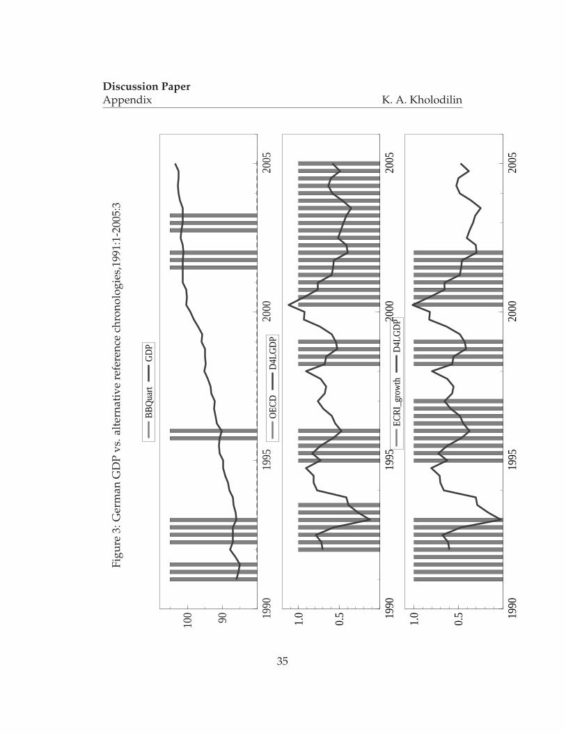
Discussion PaperAppendix K. A. Kholodilin
Figu
re3:
Ger
man
GD
Pvs
.alt
erna
tive
refe
renc
ech
rono
logi
es,1
991:
1-20
05:3
1990
1995
2000
2005
90100
BB
Qua
rt G
DP
1990
1995
2000
2005
0.5
1.0
OEC
D
D4L
GD
P
1990
1995
2000
2005
0.5
1.0
ECR
I_gr
owth
D
4LG
DP
35

Discussion PaperAppendix K. A. Kholodilin
Figu
re4:
Brit
ish
GD
Pvs
.alt
erna
tive
refe
renc
ech
rono
logi
es,1
986:
1-20
05:3
1985
1990
1995
2000
2005
2000
00
2500
00
3000
00B
BQ
uart
GD
P
1985
1990
1995
2000
2005
0.5
1.0
OEC
D
D4L
GD
P
1985
1990
1995
2000
2005
0.5
1.0
ECR
I_gr
owth
D
4LG
DP
36

Discussion PaperAppendix K. A. Kholodilin
Figu
re5:
Fren
chC
LIan
dC
CIi
nle
vels
,199
2:1-
2005
:4
1995
2000
2005
−50510(a
) Lin
ear d
ynam
ic s
ingl
e−fa
ctor
mod
els
CLI
C
CI
1995
2000
2005
−50510(b
) Dyn
amic
bi−
fact
or m
odel
with
Mar
kov
switc
hing
CLI
2f_m
s C
CI2
f_m
s
37

Discussion PaperAppendix K. A. Kholodilin
Figu
re6:
Rec
essi
onpr
obab
iliti
esof
the
sing
le-a
ndbi
-fac
tor
mod
els
for
Fran
cevs
.cyc
lical
chro
nolo
gyof
the
OEC
D,1
992:
1-20
05:4
1995
2000
2005
0.5
1.0
OEC
D
p_fC
LI
p_fC
CI
1995
2000
2005
0.5
1.0
OEC
D
p_sC
LI
p_sC
CI
1995
2000
2005
0.5
1.0
OEC
D
p_bi
fCLI
p_
bifC
CI
1995
2000
2005
0.5
1.0
OEC
D
p_bi
sCLI
p_
bisC
CI
38

Discussion PaperAppendix K. A. Kholodilin
Figu
re7:
Rec
essi
onpr
obab
iliti
esof
the
sing
le-a
ndbi
-fac
tor
mod
els
for
Fran
cevs
.cyc
lical
chro
nolo
gyof
the
ECR
I(gr
owth
cycl
e),1
992:
1-20
05:4
1995
2000
2005
0.5
1.0
ECR
I_gr
owth
p_
fCLI
p_
sCLI
1995
2000
2005
0.5
1.0
ECR
I_gr
owth
p_
fCC
I p_
sCC
I
1995
2000
2005
0.5
1.0
ECR
I_gr
owth
p_
bifC
LI
p_bi
sCLI
1995
2000
2005
0.5
1.0
ECR
I_gr
owth
p_
bifC
CI
p_bi
sCC
I
39

Discussion PaperAppendix K. A. Kholodilin
Figu
re8:
Rec
essi
onpr
obab
iliti
esof
the
sing
le-a
ndbi
-fac
tor
mod
els
for
Fran
cevs
.cyc
lical
chro
nolo
gyof
the
BBQ
(cla
ssic
alcy
cle)
,199
2:1-
2005
:4
1995
2000
2005
0.5
1.0
BB
Q
p_fC
LI
p_sC
LI
1995
2000
2005
0.5
1.0
BB
Q
p_fC
CI
p_sC
CI
1995
2000
2005
0.5
1.0
BB
Q
p_bi
fCLI
p_
bisC
LI
1995
2000
2005
0.5
1.0
BB
Q
p_bi
fCC
I p_
bisC
CI
40

Discussion PaperAppendix K. A. Kholodilin
Figu
re9:
Ger
man
CLI
and
CC
Iin
leve
ls,1
991:
1-20
05:3
1995
2000
2005
−5.0
−2.50.0
2.5
5.0
7.5
(a) L
inea
r dyn
amic
sin
gle−
fact
or m
odel
sC
LI
CC
I
1995
2000
2005
05
(b) D
ynam
ic b
i−fa
ctor
mod
el w
ith M
arko
v sw
itchi
ngC
LI2f
_ms
CC
I2f_
ms
41

Discussion PaperAppendix K. A. Kholodilin
Figu
re10
:Rec
essi
onpr
obab
iliti
esof
the
sing
le-a
ndbi
-fac
torm
odel
sfo
rGer
man
yvs
.cyc
lical
chro
nolo
gyof
the
OEC
D,1
991:
1-20
05:3
1995
2000
2005
0.5
1.0
OEC
D
p_fC
LI
p_fC
CI
1995
2000
2005
0.5
1.0
OEC
D
p_sC
LI
p_sC
CI
1995
2000
2005
0.5
1.0
OEC
D
p_bi
fCLI
p_
bifC
CI
1995
2000
2005
0.5
1.0
OEC
D
p_bi
sCLI
p_
bisC
CI
42

Discussion PaperAppendix K. A. Kholodilin
Figu
re11
:Rec
essi
onpr
obab
iliti
esof
the
sing
le-a
ndbi
-fac
torm
odel
sfo
rGer
man
yvs
.cyc
lical
chro
nolo
gyof
the
ECR
I(gr
owth
cycl
e),1
991:
1-20
05:3
1995
2000
2005
0.5
1.0
ECR
I_gr
owth
p_
fCLI
p_
sCLI
1995
2000
2005
0.5
1.0
ECR
I_gr
owth
p_
fCC
I p_
sCC
I
1995
2000
2005
0.5
1.0
ECR
I_gr
owth
p_
bifC
LI
p_bi
sCLI
1995
2000
2005
0.5
1.0
ECR
I_gr
owth
p_
bifC
CI
p_bi
sCC
I
43

Discussion PaperAppendix K. A. Kholodilin
Figu
re12
:Rec
essi
onpr
obab
iliti
esof
the
sing
le-a
ndbi
-fac
torm
odel
sfo
rGer
man
yvs
.cyc
lical
chro
nolo
gyof
the
BBQ
(cla
ssic
alcy
cle)
,199
1:1-
2005
:3
1995
2000
2005
0.5
1.0
BB
Q
p_fC
LI
p_sC
LI
1995
2000
2005
0.5
1.0
BB
Q
p_fC
CI
p_sC
CI
1995
2000
2005
0.5
1.0
BB
Q
p_bi
fCLI
p_
bisC
LI
1995
2000
2005
0.5
1.0
BB
Q
p_bi
fCC
I p_
bisC
CI
44

Discussion PaperAppendix K. A. Kholodilin
Figu
re13
:Bri
tish
CLI
and
CC
Iin
leve
ls,1
986:
1-20
05:3
1990
1995
2000
2005
−505
(a) L
inea
r dyn
amic
sin
gle−
fact
or m
odel
sC
LI
CC
I 1990
1995
2000
2005
−505
(b) D
ynam
ic b
i−fa
ctor
mod
el w
ith M
arko
v sw
itchi
ngC
LI2f
_ms
CC
I2f_
ms
45

Discussion PaperAppendix K. A. Kholodilin
Figu
re14
:R
eces
sion
prob
abili
ties
ofth
esi
ngle
-an
dbi
-fac
tor
mod
els
for
UK
vs.
cycl
ical
chro
nolo
gyof
the
OEC
D,1
986:
1-20
05:3
1990
1995
2000
2005
0.5
1.0
OEC
D
p_fC
LI
p_fC
CI
1990
1995
2000
2005
0.5
1.0
OEC
D
p_sC
LI
p_sC
CI
1990
1995
2000
2005
0.5
1.0
OEC
D
p_bi
fCLI
p_
bifC
CI
1990
1995
2000
2005
0.5
1.0
OEC
D
p_bi
sCLI
p_
bisC
CI
46

Discussion PaperAppendix K. A. Kholodilin
Figu
re15
:R
eces
sion
prob
abili
ties
ofth
esi
ngle
-an
dbi
-fac
tor
mod
els
for
UK
vs.
cycl
ical
chro
nolo
gyof
the
ECR
I(gr
owth
cycl
e),1
986:
1-20
05:3
1990
1995
2000
2005
0.5
1.0
ECR
I_gr
owth
p_
fCLI
p_
sCLI
1990
1995
2000
2005
0.5
1.0
ECR
I_gr
owth
p_
fCC
I p_
sCC
I
1990
1995
2000
2005
0.5
1.0
ECR
I_gr
owth
p_
bifC
LI
p_bi
sCLI
1990
1995
2000
2005
0.5
1.0
ECR
I_gr
owth
p_
bifC
CI
p_bi
sCC
I
47

Discussion PaperAppendix K. A. Kholodilin
Figu
re16
:R
eces
sion
prob
abili
ties
ofth
esi
ngle
-an
dbi
-fac
tor
mod
els
for
UK
vs.
cycl
ical
chro
nolo
gyof
the
BBQ
(cla
ssic
alcy
cle)
,198
6:1-
2005
:3
1990
1995
2000
2005
0.5
1.0
BB
Q
p_fC
LI
p_sC
LI
1990
1995
2000
2005
0.5
1.0
BB
Q
p_fC
CI
p_sC
CI
1990
1995
2000
2005
0.5
1.0
BB
Q
p_bi
fCLI
p_
bisC
LI
1990
1995
2000
2005
0.5
1.0
BB
Q
p_bi
fCC
I p_
bisC
CI
48