the u.s. business cycle, 1865-1939: dynamic factor analysis vs...
TRANSCRIPT

The U.S. Business Cycle, 1865-1939:
Dynamic Factor Analysis vs.
Reconstructed National Accounts
Albrecht Ritschl Humboldt University of Berlin
Samad Sarferaz Humboldt University of Berlin
Martin Uebele Humboldt University of Berlin
September 15, 2006
Abstract
This paper presents insights on the American business cycle during the pre- and interwar periods derived from disaggregate diffusion indices. We employ a Bayesian approach to dynamic factor analysis, and obtain factors representing economic activity in the U.S. economy across the divides of World War I and the Great Depression. We find a remarkable increase in volatility across World War I, which is even stronger than suggested by Romer (1987, 1989) from a re-examination of Historical National Accounts. Extending our results across World War II, we find that the post-war moderation in aggregate volatility occurred only relative to the interwar period but not with regard to the rather mild fluctuations we find before World War I. Our estimates also broadly confirm the NBER business cycle chronology for the prewar and interwar period.
Keywords: U.S. business cycle, volatility, dynamic factor analysis
JEL codes: N11, N12, C43, E32

1. Introduction Measuring the American business cycle during the pre- and interwar period has been
the subject mater of controversial debate. While there is broad agreement on the
business cycle turning points, the issue of volatility is still not fully resolved, as
different available estimates yield contradictory results. Did business cycle volatility
increase markedly after World War I? Is there a moderation after World War II, not
just with respect to the interwar period but also compared to the prewar years? How
severe were the key recessions other than the Great Depression of the 1930s, that is,
the recessions of the mid 1880s, of 1907, and of 1920/21?
Research on these issues has largely focused on the quality of Historical
National Accounts (HNA) and the scope for their improvement. For the half-century
before 1929 when the official National Income and Product Accounts (NIPA) set in,
mainly two GNP series have been in use, an official series generated by the
Commerce Department and the alternative Kendrick (1961) estimates (see Romer,
1988 for a detailed discussion and an explanation of their connection to earlier work
by Kuznets (1941), Kuznets (1946)). Both series are essentially indices that employ
different weighing and deflating schemes (one being weighed using 1982 prices, the
other using 1929 prices). Balke and Gordon (1986), Balke and Gordon (1989)
produced a revision and a widely used quarterly interpolation of the Commerce series.
Romer (1988), Romer (1989) presented a revised Kendrick series, which combined
income and product estimates of GNP to obtain an estimate that she argued was
unlikely to exhibit systematic bias in volatility vis-a-vis the true unknown data. For
both the pre- and interwar period, the series she obtained is markedly less volatile
than the Commerce series and the Balke/Gordon estimate derived from it. However,
no strategy has been devised as yet to make her calculations, as well as the underlying

plausibility considerations she presented, empirically testable. Doing this is one
objective of the present paper.
Intertemporal comparisons of volatility by HNA also hinge on comparable
data coming from a consistent source. Using comparable historical series across the
World Wars, Romer (1986) argued that no major reduction in volatility from the pre-
WWI to the postwar period could be found. The empirical basis for such comparisons
necessarily remains narrow, dictated by the availability of series that cover
sufficiently long spans on a consistent methodological basis. Again, the issues is
whether a testing strategy can be derived that makes the most efficient possible use of
the sparse information available.
The present paper takes up these debates and offers an alternative but
complementary approach. We draw on the growing literature on diffusion indices
(using a term of Stock and Watson (2002)) of economic activity, which are distilled
from a large panel of disaggregate time series using dynamic factor analysis. Stock
and Watson (1991) note that for a set of over a 100 disaggregate series representing
the U.S. postwar economy, these indices reliably replicate the NBER’s business cycle
turning points, as well as the stylized facts about business cycle intensity. In the
present paper, we adopt a Bayesian version of this methodology1 and apply it to a
wealth of disaggregate historical time series, taken mostly from the NBER’s
Macrohistory Database (which itself dates back to the business cycle project of Burns
and Mitchell (1947)). We look at the evolution of volatility over time on the basis of
different subsets of our data, and alternating between constant and time-varying
coefficients.
1 See e.g. Stock and Watson (2005) for a review.

The basic idea of this approach is to replace the aggregation techniques used in the
construction of HNA with a statistical algorithm, where the aggregation exploits the
information in the contemporaneous variance/covariance matrix of a large array of
disaggregate indicator series. To our knowledge, this approach was first applied in the
context of presenting an alternative to HNA estimates by Gerlach and Gerlach-Kristen
(2003) for Switzerland between the 1880s and the Great Depression. Sarferaz and
Uebele (2006) employ a Bayesian version of this approach to obtain an index of
economic activity for 19th century Germany that helps to decide between different
rivaling HNA-based chronologies. The present paper extends this methodology to the
historical application of macroeconomic diffusion indices with time-varying factor
loadings.
Our findings on changes in historical business cycle volatility are even more
dramatic than Romer’s. We picture the pre-World War I economy as probably even
less volatile than her estimates would suggest, and reaffirm the results that the
postwar business cycle was no less volatile than the fluctuations of the late 19th
century. At the same time, we reopen the case for a sharp real recession around 1920
that seemed settled through Romer’s (1988) work. Introducing identifying restrictions
to distinguish between real and nominal factors, we find minimal volatility of
monetary and financial conditions in the 19th century but a massive increase after
1914, supporting the popular claim that the establishment of the Federal Reserve
System in 1914 had negative, if any, effects on the stability of the U.S. monetary and
financial system.
The remainder of the paper is structured as follows. The next section briefly
sketches the main ingredients of the factor model we employ. Section III, divided up
in several subsections, presents the evidence. Section IV concludes.

II. Theory Dynamic factor models in the vein of Sargent and Sims (1999), Geweke (1977) and
Stock and Watson (1989) comprise that a given dataset can be divided into a latent
common part, which captures the comovements of the cross section and a variable
specific idiosyncratic part. These models imply that the economic activity is driven by
some few latent driving forces, which can be revealed by the estimation of the
dynamic factors. A Bayesian approach to DFMs is provided by Otrok and Whiteman
(1998), Kim and Nelson (1999) and Kose, Otrok and Whiteman (2003). Del Negro
and Ortok (2004) provide the estimation procedure for dynamic factor models with
time-varying parameters. For the estimation of the time-invariant parameters, we use
the methods described in Kim and Nelson (1999), because we condition on the first p
initial observations.
Our panel of data ity , spanning a cross section of Ni ,,1 K= series and an
observation period of length T, can be described by the following equation:
tittiiti ufcy ,,, ++= λ
where tf represents the latent factor, ic is the constant term, ti ,λ is the coefficient
linking the common factor to the i-th variable at time t, and tiu , is the variable-
specific idiosyncratic component. For the factor we assume an AR(q) process:
tqtqtt fff υφφ +++= -1-1 K
The law of motion for the idiosyncratic shock tiu , is expressed as:

tiptiptiti uuu ,-,1-,1, χθθ +++= K
and the factor loadings are assumed to be either constant or (in the time-varying
model) follow a driftless random walk:
tititi ,1-,, ελλ +=
The disturbances ti,χ , ti,ε , tv are i.i.d. normal.
The factors in this model are identifies up to a scaling constant and a sign restriction.
The scale indeterminacy can be tackled by fixing the variance of the factor
innovations tυ to be equal to a constant (see e.g. Sargent and Sims, 1977). We deal
with the sign indeterminacy of the factor loadings ti,λ and the factors tf by
restricting one of the factor loadings to be positive (see Geweke and Zhou, 1996).
Neither of these two identification assumptions restricts the information content of the
factor model.
We estimate the model in Bayesian fashion via the Gibbs sampling approach.
This procedure enables the researcher to draw from nonstandard distributions by
splitting them up into several blocks of standard conditional distributions. In our
case, the estimation procedure is subdivided into three blocks: First, the parameters of
the model },,,{ rsc θφ for prqs ,,1and,,1 KK == are calculated. Second,
conditional on the estimated values of the first block, the factor tf is computed.
Finally, conditional on the results of the previous blocks we estimate the (possibly
time-varying) factor loadings. All blocks are calculated by applying the methods
described in Kim and Nelson (1999). After the estimation of the third block, we start
the next iteration step again at the first block by conditioning on the last iteration step.

If the number of iteration steps goes to infinity, then it can be shown that the
conditional posterior distributions of the parameters and the factor will converge to
their marginal posterior distributions at an exponential rate2.
Similar to Del Negro and Otrok (2004) we use the cross section mean of the
factor loadings ∑=
=N
i tit N 1 ,
1λλ as an approximation for the change in volatility of
the dataset.
The prior for the autoregressive parameters is similar to the conjugate prior
applied by Kose, Otrok and Whiteman (2003), where the prior mean is equal to zero
and the covariance matrix is the diagonal matrix )1
1,
21
,1(diag=Σp
K , which
implies that we give more distant lagged values less weight. For the prior on the
variances of the idiosyncratic components we follow Otrok and Whiteman (1998),
which is Inverted Gamma(6,0.001). As in Del Negro and Otrok (2004), the prior on
the variances of the disturbances in the factor loadings law of motion is chosen to be
relatively tight.
III. Empirical Results
(a) 1869-1929, Constant Factor Loadings
We begin with the comparison of volatility between the prewar and interwar period.
As discussed above, factors are identified only up to a scaling factor (and a sign
convention, which is innocuous). Hence, comparisons of volatility can only be made
conditional on prior calibration. We implement this throughout by calibrating our
2 See Geman and Geman (1984).

series to the standard deviation of the (annualized) Balke and Gordon (1986) series
from their Hodrick/Prescott[6,25]-filtered trend. In a first step of our analysis, we
obtain a factor of general economic activity imposing constant factor loadings, as is
standard. The factor loads on 52 series, of which 32 can be categorized as real, while
another 20 are nominal. Most data are from the NBER Macroeconomic History
Database; some additional series we inserted from the newest edition of the Historical
Statistics of the U.S.3 Appendix A provides a list of variables.
(Figures 1a and 1b about here)
Results in Figure 1a show the factor, the simulated 67% upper and lower confidence
bands, as well as the original Balke and Gordon (1986, 1987) version of the
Commerce GNP series for 1869 to 1929. By construction, the factor and the Balke-
Gordon series have the same volatility for the sample period as a whole. We note that
both series, in spite of the vastly different methods of their calculation, tell broadly the
same business cycle chronology. Figure 1b includes the factor and the 2/3 confidence
bands, plotted against Romer’s (1986, 1989) version of the Kuznets/Kendrick GNP
estimate for the same observation period. Again, the factor paints broadly the same
picture in terms of the business cycle chronology it implies.
Differences between the HNA estimates of GNP and the factor, however,
appear to exist in volatility. Unsurprisingly, the factor is on the whole more volatile
than Romer’s series. This is so by construction, reflecting the higher overall volatility
of the Balke/Gordon estimate. We are interested instead in comparing the ehavior of
volatility across the divide of World War I.
3 See Carter, Gartner, Haines, Olmstead, Sutch and Wright (2006).

(Table 1 about here)
As Table 1 bears out, both the Balke/Gordon and Romer estimates of GNP show an
increase in volatility across World War I. This effect is stronger in the Balke/Gordon
estimate, largely because it exhibits a much sharper recession in 1920/21 than the
Romer series. Comparing the factor estimnates to the datam, we obtain an even
stronger increase in volatility across World War I than the Balke/Gordon estimate.
This has two implications. First, even if we accept the higher overall volatility of the
Balke/Gordon estimate for the observation period as a whole, the volatility of
economic activity before World War I was lower than their series implies – which
reinforces a claim made by Romer (1988, 1989) on the basis of new HNA re-
estimates.
However, we also see that by all means, our factor shows very high volatility
for the 1920s. Indeed, the factor appears to reinstate the 1920/21 recession, which
looked severe in the traditional Commerce estimate of GNP (and hence in
Balke/Gordon) but rather less severe in the Kendrick (1961) estimates and their
adaptation by Romer (1986, 1989). We find this effect to be noticeable, as it seems to
put a question mark between the assertion of Romer (1988) that the volatility of the
Balke/Gordon series in the 1920s is an artifact caused largely by employing 1982
prices in their weighing scheme. Our factor is rich in contemporary price information
and avoids any mechanistic aggregation that might generate spurious volatility.
Hence, it is immune against this critique. In the following subsections, we will
therefore subject both results – lower volatility pre-1914, increased volatility
thereafter – to further scrutiny.

(b) 1869-1914 – Expanded Dataset
The first step is to look into the prewar period in greater detail, and to see if there are
any major changes in volatility within this subperiod. The attempt to compare
volatility across World War I required narrowing the available dataset to 52 series that
are available for the whole period from 1869 to 1929. One salient feature of the pre-
war business cycle as represented in Figure 1 above seems to be the time variation of
volatility. As the factor was extracted from the common component of the underlying
time series for both the pre-war and the interwar period, any dynamics pertinent to the
latter but not to the former might be carried over and distort the business cycle
measurement for the prewar years. We therefore repeated extracting the common
component from the same 52 series for the pre-war period only (Figure 2a).
(Figure 2a about here)
As can be seen, results differ somewhat from the common factor for the longer period,
bu the main patterns are preserved: there is a strong upswing in the early 1870s,
followed by a recession in the second half of the decade, as well as a second recession
in 1885 and an intermittent upswing. The recessions of 1894, 1904, and 1907 are also
clearly visible. Eyeballing would again suggest that in terms of turning points, the fit
with the Balke/Gordon series is somewhat better.
(Figure 2b about here)

As an alternative to this benchmark, in Figure 2b we look at a factor extracted from an
expanded dataset of 103 series, which provide a much broader coverage of the U.S.
economy. Calculation of this broader factor exhibits two main results: first, all
recessions and upswings except for 1906/1907 now seem to be of more or less equal
intensity; the evidence from Figures 1 and 2a of more intense fluctuations prior to
1890 disappears. Secondly, however, the factor is estimated only very imprecisely. A
look at the error bands suggests the possibility of severe recessions in 1878, 1885 and
– newly – 1891 as well as 1898, while the evidence for the 1894 recession becomes
much weaker.
Hence, broadening the dataset seems to come at a cost, as the many additional
series appear to introduce considerable additional noise, which the model finds hard
to deal with. A tentative conclusion from the broader evidence seems warranted,
however: prior to 1905, the evidence for major shifts in the volatility of the U.S.
business cycle is at best mixed. The one recession that stands out from the pre-1914
evidence is the sharp contraction of 1907. It seems to initiate a pattern that became
typical of the interwar business cycle.
(c) 1869-1929: Time-Varying Factor Loadings
An alternative to broadening the dataset that allows making volatility comparisons
across World War I is to allow factor loadings to vary. As laid out before, time-
varying factor loadings render it possible to capture structural changes that affect the
interplay between sectoral and aggregate dynamics. The analogy is with an index
number (which is what the factor actually is). Making the factor loadings variable is

then analogous to allowing the index weights to change over time4. Proceeding this
way with our 52 series across World War I, we obtain a striking confirmation of our
previous results.
(Figures 3a and 3b about here)
Figure 3 shows a time-varying factor of economic activity for the period of 1869 to
1929, along with the Balke/Gordon and Romer estimates of GNP5. This factor is
remarkably flatter than both the Balke/Gordon and Romer series for pre-1914.
eyeballing suggests that during this period, its turning points are now closer to the
Romer series, whereas the cyuclical movements of the constant factor shown in
Figures 1a and 1b above seemed closer to the Balke/Gordon series. We find this result
to be noticeable, as it reflects romer’s criticism of indices with constant weights as
exaggerating volatility: as soon as we allow index weights to vary, much of the
volatility in the factor disappears, suggesting it was spurious in the first place. The
principal innovation here is that we do not do this by introducing a priori information
from e.g. census data, as would be common in conventional HNA construction, but
rather by likelihood methods that invoke the information content in the changing
cross-covariance of a large number of disaggregate series.
However, we again do not find a reduction in volatility after 1914. The time-
varying factor now fluctuates wildly and is very close to the Balke/Gordon series,
4 Note, however, that the factor loadings, whether time-varying or not, do not have the same economic interpretation as conventional index weights. While the latter typically represent employment, value added, or expenditure shares, the factor loadings are determined optimally from the iterating on the estimated joint distribution of factor loadings and data.
5 The observations before 1880 get used up by a “training sample” required for initiating the prior. Graphing them would thus carry no information.

except for the 1920/21 recession where it is even more volatile. Thus, our analysis
seems to conform with the traditional hypothesis of violent aggregate fluctuations
after World War I, which is not reflected in the Kendrick (1961) and Romer (1988)
estimates of GNP.
(Table 2 about here)
Table 2 summarizes the volatility results for the time-varying factor, again calibrated
to the Balke/Gordon series. As it turns out, the standard deviation for pre-1914 is now
down to almost half the level of the Romer series, while it is significantly higher than
bothe GNP series for the interwar period.
We conclude from this exercise that the higher volatility of the so-called Commerce
series and its adaptation by Balke and Gordon (1986, 1987) is not primarily a problem
of too narrow data representation or aggregation by the wrong price vector. We were
able to generate rather volatile indices of economic activity for the 19th century using
constant factor loadings from a rather broad set of data (in Figure 1 above) that suffers
from neither of the criticisms raised against this series. Instead, we find that changing
sectoral weights seem to be the major problem plaguing the data before World War I.
As soon as we allowed the factor loadings to vary, we were able to generate an
outcome that is markedly less volatile than even the Kendrick/Romer estimate of GNP
for the pre-war period. This finding would not be easy to obtain with HNA methods,
as the necessary census information on changing sectoral index weights is only
seldom available at sufficiently high levels of quality and observation frequency, and
certainly not for the U.S. prior to World War I.

(d) Structural Factors: Real vs. Nominal
In this subsection, we refine the analysis to account for real and nominal influences
separately. The literature on factor analysis of economic activity is divided on how to
do this best: a non-structural approach is to extract more than one factor from the full
dataset, forcing the second factor to be orthogonal to the first one. This procedure is
generally seen as yielding good characterizations of real activity by the first factor,
and of nominal conditions by the second factor. A more structural alternative to be
followed here is to restrict factor loadings a priori by exclusion restrictions. We do
this in Figure 4 for 1880 to 1929.
(Figure 4 about here)
Results for the real factor (Figure 4a) seem reassuring. The Great Depression of the
1880s appears back on stage, as do the 1904 and 1906 recessions. We also see the
wartime boom and post-World War I recession in the data very clearly. The late
1920s also show a sharp economic expansion, an effect that was not visibile in any of
the existing GNP estimates, but that does show up in the index of industrial
production by Miron and Romer (1990). An exciting message is delivered by the
nominal factor shown in Figure 4b: while the 19th century is essentially flat in
nominal shocks to the U.S. economy, very marked shocks appear during World War I.
The postwar deflation is clearly visible (if a bit belated), as is the nominal expansion
of the late 1920s. hence, both real and nominal volatility increased greatly across
World War I, the latter even more strongly so than the former.
Several tentative conclusions suggest themselves. First, it seems safe to rule
out major monetary causes of the pre-war recessions. Neither are the nominal

impulses very strong nor does the timing (in the sense of Granger causation) seem to
be right. Second, monetary shocks gain greatly in size but not in significance after
World War I. Again, timing seems to be a problem. Third, the evidence sheds an
unfavorable light on the performance of the Federal Reserve System after its
establishment in 1914: while the classical gold standard apparently did not too badly
in smoothing out nominal shocks, its more managed version does not look impressive
at all.
We again extend the analysis to 1939, keeping in mind, however, that the
estimates are not recursive, such that the estimated factor loadings for any point in
time t are potentially affected by extending the observation period from T to T+S.
Results are shown in Figure 5.
(Figure 5 about here)
As Figure 5 bears out, taking the Great Depression of the 1930s on board tends to
dampen the previous swings somewhat, and also to affect their timing. Notably, the
real expansion during World War I now looks weaker, and the postwar recession is
shifted backwards by one year. The nominal swings, in contrast, come out sharper and
much more significantly as far as the post-1914 years are concerned. As to the Great
Depression, the nominal turning point is now in 1929 (influenced also by the stock
market index that is enters the nominal factor), while the real turning point is –
somewhat implausibly – in 1931. Again, this shows how strongly the results are
affected by the non-recursive nature of the estimates: a contemporary observer
somehow informed by the Great Depression would have inferred since World War I
that monetary shocks were pervasive and significant. For an agent updating the
information set recursively in real time, this was probably not at all clear, as the low
significance levels of the factors obtained till 1929 show. This shows how important it
is to avoid statements on policy effectiveness from non-recursive estimates if the
underlying structures are not time-invariant6.
(e) Long-Term Volatility of U.S. Economic Activity
Our analysis of historical business cycle volatility can also be extended to the long run
of over a century, albeit on a narrow database. In this subsection we present evidence
based on a consistent set of 14 time series that wer recorded since 1890 on an
unchanged basis, and that are readily available. Evidently, the problem of inadequate
data representation becomes a big one over such a long period, and is unlikely to be
mitigated by the choice between constant and time-varying factor loadings.
(Figures 6 a and b about here)
As can be seen from Figure 6, some clear patterns emerge despite the unavoidable
data limitations. Most importantly, the increase in volatility during the interwar period
is clearly reflected in the data, as is the Great Moderation of U.S. aggregate
fluctuations after World War II. We do find it notable, though, that the levels of 19th
century volatility are not reached again until the 1960s. We also observe recurrent
volatility since the mid-1970s, an effect that is not borne out by modern GNP series
for the U.S. We have no doubt that this evidence is generated by the heavy
dependence of our factors on raw material production and financial indicators, whose
6 Amir Ahmadi and Ritschl (2006) have a factor model of monetary policy transmission on the interwar U.S. economy, and find only very minor effects.

high volatility in the last decades of the 20th century is undisputed. Clearly, however,
the postwar business cycle as reflected in our factor was no less volatile than the pre-
World War I cycle, which confirms a result of Romer (1986).
IV. Conclusions Factor analysis of aggregate economic activity presents an appealing alternative to
Historical National Accounts whenever the data are incomplete or plagued by
structural breaks in reporting. In this paper, we re-examined the volatility of historical
business cycles in the U.S. since 1869. While focusing mostly on the comparison
between the pre-war and the interwar period, we also presented a long-term
perspective from the late 19th century to the late 1990s.
Our main findings are that the business cycle prior to World War I was even
less volatile than has previously been thought, and was quite plausibly no more
volatile than the postwar business cycle of the 1950s. We also find pervasive evidence
that the interwar years, in particular the period immediately following World War I,
were more volatile than has been maintained in the more recent literature. This would
make the Great Depression of the 1930s less of a historical singularity.
Many of our findings derive from the analysis of time variation in factor
loadings, or the weights assigned to the various individual series in constructing the
index of aggregate economic activity. To this end, we employed a Bayesian approach
to factor analysis, iterating over the likelihood function by Gibbs sampling. We found
time varying factor loadings to be an effective way of dealing with the structural
changes in the U.S. economy, a problem that is hard to deal with in HNA approaches.
As a result, we suspect that spurious volatility in national accounts of the U.S.
business cycle is not so much a problem of missing or too narrow data but rather of

the inflexible weighing schemes underlying most work in national accounting with
historical data.
We also took a more structural approach, restricting our data to load into one
real and one nominal factor separately. While the real factor replicates the well-
known business cycle turning points without problems, the nominal factor shows only
very minor movements in the 19th century. Viewed in this perspective, the creation of
the Federal Reserve System in 1914 had apparently no stabilizing influence on the
monetary and financial system of the U.S. economy. Whether it also affected
economic activity in the U.S. in the long run is an issue for further research7
References
Amir Ahmadi, Pooyan, and Albrecht Ritschl, 2006. Monetary Policy During the Great Depression: A Bayesian FAVAR Approach (mimeo, Humboldt University of Berlin).
Balke, Nathan, and Robert Gordon, 1986, Appendix: Historical Data, in R. Gordon, ed.: The American Business Cycle (University of Chicago Press, Chicago).
Balke, Nathan, and Robert Gordon, 1989, The Estimation of Prewar Gross National Product: Methodology and New Evidence, Journal of Political Economy 97, 84-85.
Burns, Arthur F., and Wesley C. Mitchell, 1947. Measuring Business Cycles (NBER, New York).
Carter, Susan, Scott Sigmund Gartner, Michael R. Haines, Alan R. Olmstead, Richard Sutch, and Gavin Wright, eds., 2006. Historical Statistics of the United States. Millenium Edition (Cambridge University Press, New York).
Gerlach, Stefan, and Petra Gerlach-Kristen, 2003. Estimates of Real Economic Activity in Switzerland, 1886-1930 (mimeo, Hong Kong Institute of Monetary Research).
Geweke, J, 1977, The Dynamic Factor Analysis of Economic Time Series, in D.J. Aigner, and Alan D. Goldberger, eds.: Latent Variables in Socio-Economic Models (North Holland, Amsterdam).
Kendrick, John, 1961. Productivity Trends in the United States (Columbia University Press, New York).
Kim, Chang-Jin, and Charles R. Nelson, 1999. State-Space Models with Regime Switching (MIT Press, Cambridge).
7 The only truly long-term studies of monetary policy effects on the U.S. economy we are aware of are Sims (1999) and Sargent (1999). Stock and Watson (2005) provide an overview of estimates of monetary policy effectiveness in a dynamic factor framework for U.S. postwar data beginning in the late 1950s.

Kose, Ayhan, Christopher Otrok, and Charles H. Whiteman, 2003, International Business Cycles: World, Region and Country-Specific Factors, American Economic Review 93, 1216-1239.
Kuznets, Simon, 1941. National Income and Its Composition, 1919-1938 (National Bureau of Economic Research, New York).
Kuznets, Simon, 1946. National Product Since 1869 (National Bureau of Economic Research, New York).
Miron, Jeffrey A., and Christina Romer, 1990, A New Monthly Index of Industrial Production, 1884-1914, Journal of Economic History 40, 321-337.
Otrok, Christopher, and Charles H. Whiteman, 1998, Bayesian Leading Indicators: Measuring and Predicting Economic Conditions in Iowa, International Economic Review 39, 997-1014.
Romer, Christina, 1986, Is the Stabilization of the Postwar Economy a Figment of the Data?, American Economic Review 76, 314-334.
Romer, Christina, 1988, World War I and the Postwar Depression: A Reinterpretation Based on Alternative Estimates of GNP, Journal of Monetary Economics 22, 91-115.
Romer, Christina, 1989, The Pre-War Business Cycle Reconsidered: New Estimates of Gross National Product, 1869-1908, Journal of Political Economy 97, 1-37.
Sarferaz, Samad, and Martin Uebele, 2006. Tracking Down Germany's Pre-World War I Business Cycle: A Dynamic Factor Model for 1820-1913 (mimeo, Humboldt University of Berlin).
Sargent, T., 1999. The Conquest of American Inflation (Princeton University Press, Princeton).
Sargent, Thomas, and Christopher Sims, 1999, Business Cycle Modeling Without Pretending to Have Too Much A-Priori Economic Theory, in Christopher Sims, ed.: New Methods in Business Cycle Research (Federal Reserve Bank of Minneapolis, Minneapolis).
Sims, Christopher, 1999, The Role of Interest Rate Policy in the Generation and Propagation of Business Cycles: What Has Changed Since the 30s?, in Scott Shuh, and Jeffrey Fuhrer, eds.: Beyond Shocks: What Causes Business Cycles? (Federal Reserve Bank of Boston, Boston).
Stock, James, and Mark Watson, 1989, New Indexes of Coincident and Leading Economic Indicators, NBER Macroeconomics Annual 351-393.
Stock, James, and Mark Watson, 1991, A Probability Model for the Coincident Economic Indicators, in G. Moore, and K. Lahiri, eds.: The Leading Economic Indicators: New Approaches and Forecasting Records (Cambridge University Press, Cambridge).
Stock, James, and Mark Watson, 2002, Macroeconomic Forecasting Using Diffusion Indexes, Journal of Business and Economic Statistics 20, 147-162.
Stock, James, and Mark Watson, 2005, Implications of Dynamic Factor Models for VAR Analysis, mimeo.

Appendix: Data series and sources (a) 103 series, 1867-1914 1 Wholesale Price Cotton, raw 2 Oats production 3 INDEX OF CROP PRODUCTON, TWELVE IMPORTANT CROPS 4 INDEX OF TOTAL CROP PRODUCTION 5 WHEAT CROP 6 WHEAT CROP 7 POTATO CROP 8 OAT CROP 9 CORN CROP 10 COTTON CROP 11 WHEAT CROP ACREAGE 12 WHEAT CROP ACREAGE 13 POTATO CROP ACREAGE 14 OAT CROP ACREAGE 15 CORN CROP, YIELD PER ACRE 16 CORN CROP ACREAGE 17 COTTON CROP ACREAGE 18 COTTON CROP, YIELD PER ACRE 19 CATTLE SLAUGHTERED UNDER FEDERAL INSPECTION 20 TOBACCO CROP 21 TOBACCO CROP ACREAGE 22 SHEEP AND LAMBS SLAUGHTERED UNDER FEDERAL INSPECTION 23 m01038U.S. Live Hog Receipts 01/1859-12/1940 24 m04001aU.Price of Wheat, S. Wholesale , Chicago, Six Markets 07/1841-07/1944 25 m04005U.S. Wholesale Price of Corn Chicago 01/1860-12/1951 26 m04007U.S. Wholesale Price of Cattle Chicago 01/1858-12/1940 27 m04008U.S. Wholesale Price of Hogs Chicago 01/1858-12/1940 28 Wool Prices, HSUS (2006), pp3-208 29 "Population, Hist. Stat. Of the US, 2006, Vol. 3 30 Raw Steel production 31 Copper Prices,HSUS (2006), pp3-217 32 BITUMINOUS COAL PRODUCTION 33 LOCOMOTIVE PRODUCTION, BALDWIN LOCOMOTIVE WORKS 34 PIG IRON PRODUCTION 35 a02084U.S. Rail Consumption, American Iron and Steel Institute 1849-1961 36 a02244U.S. Merchant Vessels Built and Documented, Tonnage, Bureau of the Census-Customs Bureau, Annual Data 1797-1940 37 a02102U.S. U.S., Gross Tonnage of Yachts Built, Dept. Of Commerce-Bureau Of Marine Inspection and Navigation 1847-1937 38 a02135U.S. Total Merchant Marine, Annual Data Only 1843 - 1940 39 INDEX OF MANUFACTURING PRODUCTION 40 TOTAL COAL PRODUCTION 41 Brick Prices, HSUS (2006), pp3-217 42 U.S. Prices of No. 1 Anthracite Foundry Pig Iron M and N spliced 43 U.S. Wholesale Price of Copper P and Q spliced 44 Coal Prices (anthr.) 45 Coal Fuel Mineral Production 46 a02047U.S. Building Permits, Value of Total , Chicago 1854-1870, 1872-1943 47 Cargo moved on NY State canals 48 m07023U.S. Total Exports 07/1866-10/1969 49 U.S. Raw Silk Imports AA, AB and AC spliced 50 m07038U.S. Coffee Imports 01/1867-06/1941 51 m07040U.S. Tea Imports 01/1867-09/1941 52 m07042U.S. Tin Imports 01/1867-06/1893 08/1893-06/194 LONG TONS 53 m07028U.S. Total Imports 07/1866-10/1969 54 m07043aU.S. Raw Cotton Exports 01/1867-12/1941 55 Vessels entered US ports 56 Stock Prices, NBER Cowles and HSuS3-757 57 U.S. Net Savings of Life Insurance Policy Holders spliced together, NBER 58 U.S. Index of Wholesale Prices, T, U and V spliced 59 m04051U.S. Index of the General Price Level 01/1860-11/1939 60 m13001U.S. Call Money Rates Mixed Collateral 01/1857-11/1970 61 m13019U.S. American Railroad Bond Yields High Grade AT and AU spliced 62 m14124aU.S. National Bank Notes Outstanding Total End of Month 01/1864-12/1879 63 a13049U.S. Earnings Yield of All Common Stocks On the New York Stock Exchange 1871-1938 64 m13002U.S. Commercial Paper Rates New York City 01/1857-12/1971 65 US Notes 66 Business Failures 67 m12003U.S. Index of American Business Activity 01/1855-12/1970 68 m12015U.S. Bank Clearings Daily Average 10/1853-09/1943 69 Patents granted 70 a10030U.S. Number of Concerns in Business 1866-1938 71 a02004U.S. Index of Value Of Total Building, Original Data, Long 1868-1939 72 a02009U.S. Value of Building Permits Per Capita, Riggleman (Current Dollars) 1830-1933 73 a02010U.S. Value of Building Permits Per Capita, As Per Cent Of Trend, Riggleman (Constant Dollars) 1830-1933 74 a02037U.S. Adjusted Index of Building Permits, New England Cities, Riggleman 1875-1933 75 a02038U.S. Adjusted Index of Building Permits, Middle Atlantic Cities, Riggleman 1875-1933 76 a02040U.S. Adjusted Index of Building Permits, East North Central Cities, Riggleman 1875-1933 77 a02041U.S. Adjusted Index of Building Permits, West North Central Cities, Riggleman 1875-1933 78 a02042U.S. Adjusted Index of Building Permits, South Central Cities, Riggleman 1875-1933 79 a02043U.S. Adjusted Index of Building Permits, Western Cities, Riggleman 1875-1933 80 a02046U.S. Brooklyn ,Value of Permits For New Buildings 1874-1935
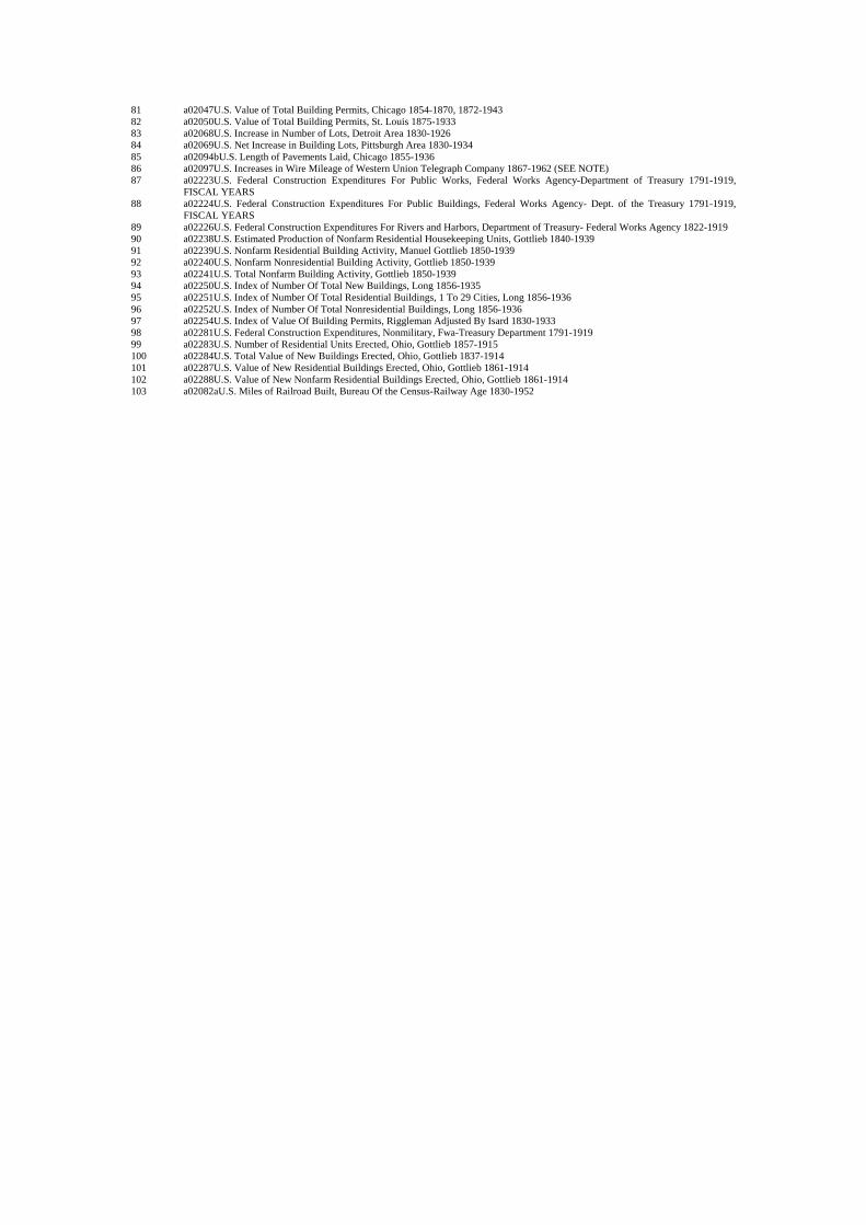
81 a02047U.S. Value of Total Building Permits, Chicago 1854-1870, 1872-1943 82 a02050U.S. Value of Total Building Permits, St. Louis 1875-1933 83 a02068U.S. Increase in Number of Lots, Detroit Area 1830-1926 84 a02069U.S. Net Increase in Building Lots, Pittsburgh Area 1830-1934 85 a02094bU.S. Length of Pavements Laid, Chicago 1855-1936 86 a02097U.S. Increases in Wire Mileage of Western Union Telegraph Company 1867-1962 (SEE NOTE) 87 a02223U.S. Federal Construction Expenditures For Public Works, Federal Works Agency-Department of Treasury 1791-1919,
FISCAL YEARS 88 a02224U.S. Federal Construction Expenditures For Public Buildings, Federal Works Agency- Dept. of the Treasury 1791-1919,
FISCAL YEARS 89 a02226U.S. Federal Construction Expenditures For Rivers and Harbors, Department of Treasury- Federal Works Agency 1822-1919 90 a02238U.S. Estimated Production of Nonfarm Residential Housekeeping Units, Gottlieb 1840-1939 91 a02239U.S. Nonfarm Residential Building Activity, Manuel Gottlieb 1850-1939 92 a02240U.S. Nonfarm Nonresidential Building Activity, Gottlieb 1850-1939 93 a02241U.S. Total Nonfarm Building Activity, Gottlieb 1850-1939 94 a02250U.S. Index of Number Of Total New Buildings, Long 1856-1935 95 a02251U.S. Index of Number Of Total Residential Buildings, 1 To 29 Cities, Long 1856-1936 96 a02252U.S. Index of Number Of Total Nonresidential Buildings, Long 1856-1936 97 a02254U.S. Index of Value Of Building Permits, Riggleman Adjusted By Isard 1830-1933 98 a02281U.S. Federal Construction Expenditures, Nonmilitary, Fwa-Treasury Department 1791-1919 99 a02283U.S. Number of Residential Units Erected, Ohio, Gottlieb 1857-1915 100 a02284U.S. Total Value of New Buildings Erected, Ohio, Gottlieb 1837-1914 101 a02287U.S. Value of New Residential Buildings Erected, Ohio, Gottlieb 1861-1914 102 a02288U.S. Value of New Nonfarm Residential Buildings Erected, Ohio, Gottlieb 1861-1914 103 a02082aU.S. Miles of Railroad Built, Bureau Of the Census-Railway Age 1830-1952

(b) 52 series, 1865 to 1939 1 Wholesale Price Cotton, raw 2 Oats production 3 m01038U.S. Live Hog Receipts 01/1859-12/1940 4 m04001aU.Price of Wheat, S. Wholesale , Chicago, Six Markets 07/1841-07/1944 5 m04005U.S. Wholesale Price of Corn Chicago 01/1860-12/1951 6 m04007U.S. Wholesale Price of Cattle Chicago 01/1858-12/1940 7 m04008U.S. Wholesale Price of Hogs Chicago 01/1858-12/1940 8 Wool Prices, HSUS (2006), pp3-208 9 Cotton production, HSUS (2006), pp4-111 10 "Population, Hist. Stat. of the U.S., 2006, Vol. 3 11 Raw Steel production 12 Copper Prices, HSUS (2006), pp3-217 13 Brick Prices, HSUS (2006), pp3-217 14 U.S. Prices of No. 1 Anthracite Foundry Pig Iron M and N spliced 15 U.S. Wholesale Price of Copper P and Q spliced 16 a02084U.S. Rail Consumption, American Iron and Steel Institute 1849-1961 17 Coal Prices (anthr.) 18 Coal Fuel Mineral Production 19 a02244U.S. Merchant Vessels Built and Documented, Tonnage, Bureau of the Census-Customs Bureau, Annual Data 1797-1940 20 a02047U.S. Building Permits, Value of Total , Chicago 1854-1870, 1872-1943 21 a02135U.S. Merchant Marine, Total , Annual Data Only 1843 - 1940 22 a02223U.S. Federal Construction Expenditures For Public Works, Federal Works Agency-Department of Treasury 1791-1919, 23 a02102U.S. Yachts Built, Gross Tonnage of , U.S., , Dept. Of Commerce-Bureau Of Marine Inspection and Navigation 1847-1937 24 a02238U.S. Nonfarm Residential Housekeeping Units, Estimated Production of , Gottlieb 1840-1939 25 a02239U.S. Nonfarm Residential Building Activity, Manuel Gottlieb 1850-1939 26 a02240U.S. Nonfarm Nonresidential Building Activity, Gottlieb 1850-1939 27 a02241U.S. Total Nonfarm Building Activity, Gottlieb 1850-1939 28 Cargo moved on NY State canals 29 m07023U.S. Total Exports 07/1866-10/1969 30 U.S. Raw Silk Imports AA, AB and AC spliced 31 m07038U.S. Coffee Imports 01/1867-06/1941 32 m07040U.S. Tea Imports 01/1867-09/1941 33 m07042U.S. Tin Imports 01/1867-06/1893 08/1893-06/194 LONG TONS 34 m07028U.S. Total Imports 07/1866-10/1969 35 m07043aU.S. Raw Cotton Exports 01/1867-12/1941 36 a02082aU.S. Miles of Railroad Built, Bureau Of the Census-Railway Age 1830-1952 37 Vessels entered US ports 38 Stock Prices, NBER Cowles and HSuS3-757 39 U.S. Net Savings of Life Insurance Policy Holders spliced together, NBER 40 a13049U.S. Earnings Yield of All Common Stocks On the NYSE 1871-1938, Boston Industrail 1866-1870, HSUS, 3-768 41 U.S. Index of Wholesale Prices, T, U and V spliced 42 m04051U.S. Index of the General Price Level 01/1860-11/1939 43 m13001U.S. Call Money Rates Mixed Collateral 01/1857-11/1970 44 m13019U.S. American Railroad Bond Yields High Grade AT and AU spliced 45 m14124aU.S. National Bank Notes Outstanding Total End of Month 01/1864-12/1879 46 m13002U.S. Commercial Paper Rates New York City 01/1857-12/1971 47 US Notes 48 Business Failures 49 a10030U.S. Number of Concerns in Business 1866-1938 50 m12003U.S. Index of American Business Activity 01/1855-12/1970 51 m12015U.S. Bank Clearings Daily Average 10/1853-09/1943 52 Patents granted
(c) 14 series, 1890-1995 1 Cotton raw 2 Oats production 3 Cotton production 4 Raw steel production 5 Cargo moved on NY state canals 6 Stock prices 7 Telephones 8 US notes 9 Coal fuel mineral production 10 Wheat prices 11 Wool prices 12 Coal prices (anthr.) 13 Copper prices 14 Brick prices

(a) vs. Balke/Gordon series (b) vs. Romer series
Fig. 1: Factor of economic activity from 52 series with 67% error bands, constant factor loadings, 1867-1914
Table 1: Volatility Increase Across World War I, Constant Factor Loadings
Std.dev. from 1869-1913 1914-1929 1869-1929 Difference RelativeHP (6.25) trend Interwar-Prewar Interwar/Prewar
Romer GNP 0.0213 0.0267 0.0225 0.0054 1.2535
Balke/Gordon GNP 0.0263 0.0390 0.0296 0.0127 1.4829
Constant Factor 52 0.0256 0.0398 0.0296 0.0142 1.5565

Fig. 2a: Factor of economic activity from 52 series with 67% error bands, constant factor loadings, 1867-1914
Fig. 2b: Factor of economic activity from 103 series with 67% error bands, constant factor loadings, 1867-1914

(a) vs. Balke/Gordon series (b) vs. Romer series
Fig. 3: Factor of economic activity from 52 series with 67% error bands, time-varying factor loadings, 1867-1914
Table 2: Volatility Increase Across World War I, Time-Varying Factor Loadings
Std.dev. from 1869-1913 1914-1929 1869-1929 Difference RelativeHP (6.25) trend Interwar-Prewar Interwar/Prewar
Romer GNP 0.0213 0.0267 0.0225 0.0054 1.2535
Balke/Gordon GNP 0.0263 0.0390 0.0296 0.0127 1.4829
TVAR Factor 52 0.0120 0.0503 0.0296 0.0383 4.1917

(a) Loading on 32 real series (b) Loading on 20 nominal series Fig. 4: Factors of economic activity from 52 series with 67% error bands, time-
varying factor loadings, 1867-1929 (a) Loading on 32 real series (b) Loading on 20 nominal series Fig. 4: Factors of economic activity from 52 series with 67% error bands, time-
varying factor loadings, 1867-1929

Fig. 5: Factors of economic activity from 14 series with 67% error bands, time-
varying factor loadings, 1890-1995