
Network Planning VITMM215
Markosz Maliosz PhD
10/05/2016
2
Outline
Telephone network dimensioning
– Traffic modeling
– Erlang formulas
– Exercises
3 3
Telephone Network
Circuit switching
Each voice channel is identical
For each call one channel is allocated
A call is accepted if at least one channel is idle
Goal: network dimensioning
Question to answer: How many circuits are required to satisfy subscribers’ needs?
Input: traffic statistics – subscribers’ behavior: when, how often are calls arriving?
how long are the call durations?
4
Arrival Process
In our case: telephone calls arriving to a switching system
described as stochastic point process
we consider simple point processes, i.e. we exclude multiple arrivals
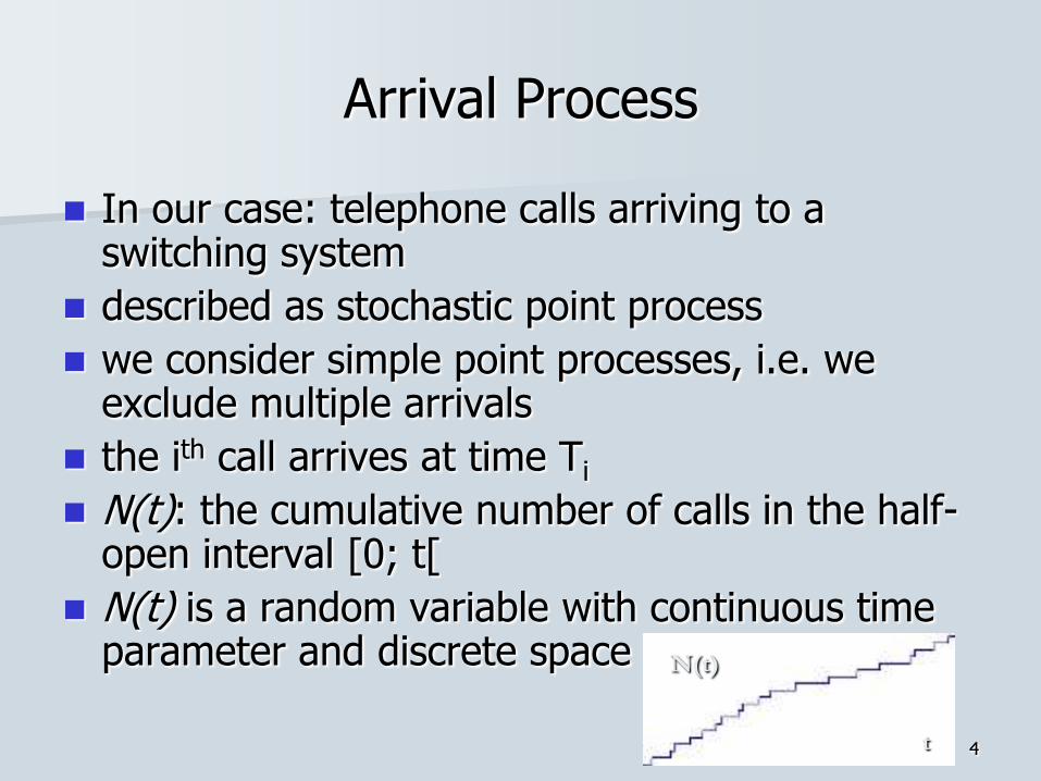
the ith call arrives at time Ti
N(t): the cumulative number of calls in the half-open interval [0; t[
N(t) is a random variable with continuous time parameter and discrete space
4 t
N(t)
5
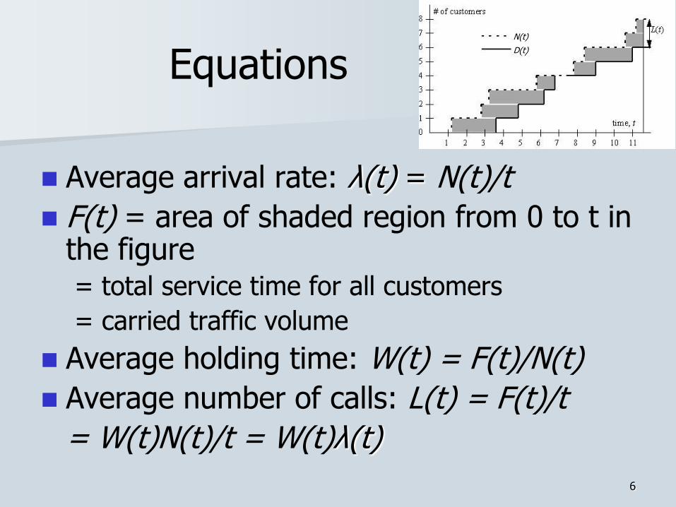
Arrivals and Departures
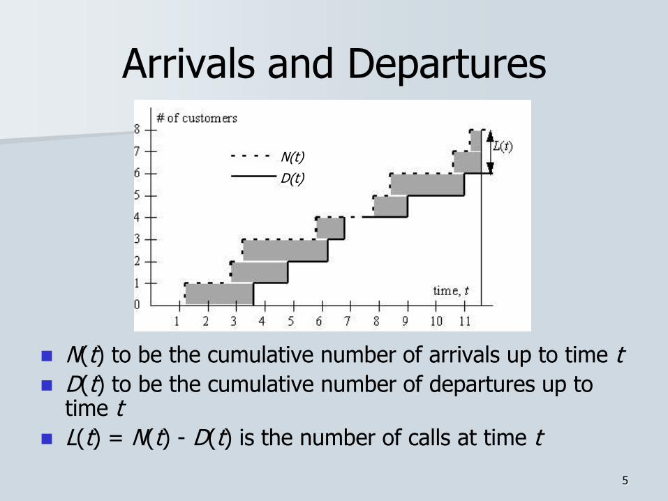
N(t) to be the cumulative number of arrivals up to time t
D(t) to be the cumulative number of departures up to time t
L(t) = N(t) - D(t) is the number of calls at time t
N(t)
D(t)
6
Equations
Average arrival rate: λ(t) = N(t)/t
F(t) = area of shaded region from 0 to t in the figure = total service time for all customers
= carried traffic volume
Average holding time: W(t) = F(t)/N(t)
Average number of calls: L(t) = F(t)/t
= W(t)N(t)/t = W(t)λ(t)
N(t)
D(t)
N(t)
D(t)
7
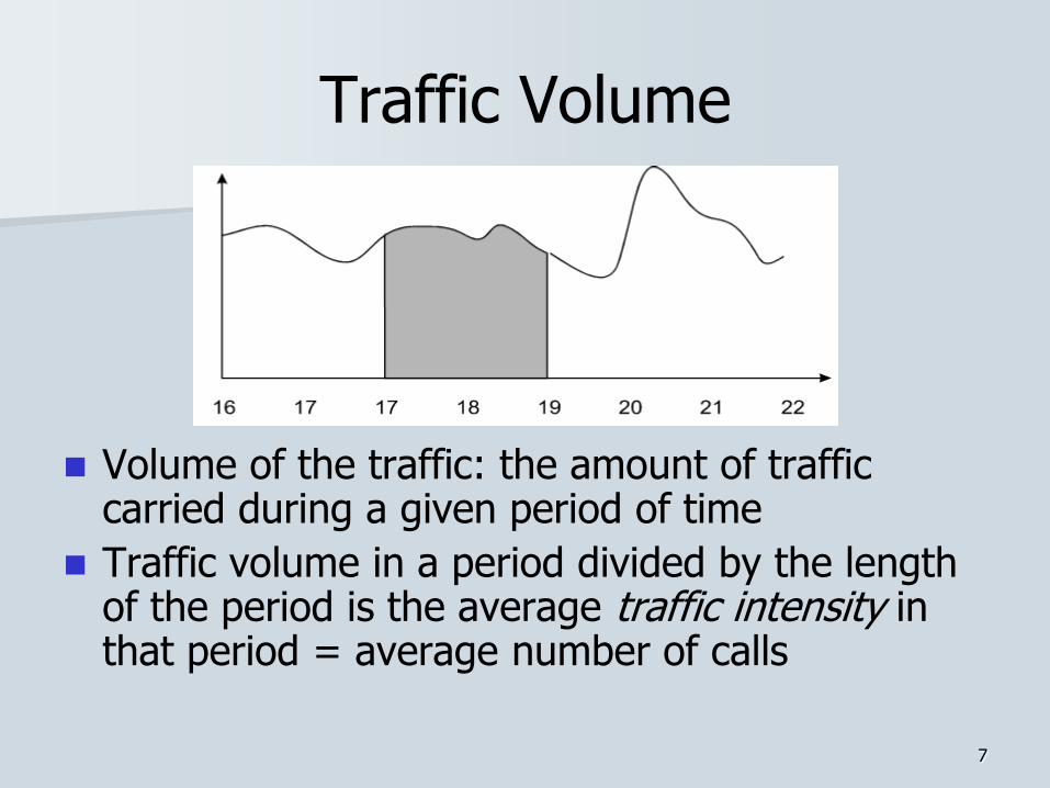
Traffic Volume
Volume of the traffic: the amount of traffic carried during a given period of time
Traffic volume in a period divided by the length of the period is the average traffic intensity in that period = average number of calls
8
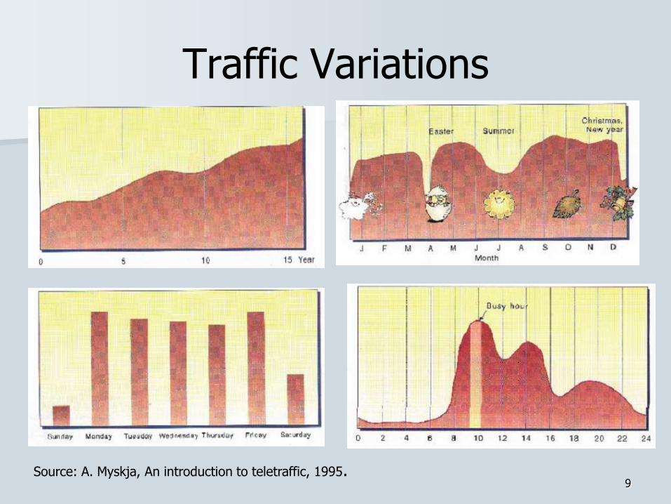
Traffic Variations
Traffic fluctuates over several time scales – Trend (>year)
Overall traffic growth: number of users, changes in usage Predictions as a basis for planning
– Seasonal variations (months) – Weekly variations (day) – Daily profile (hours) – Random fluctuations (seconds – minutes)
In the number of independent active users: stochastic process
Except the last one, the variations follow a given profile, around which the traffic randomly fluctuates
9
Traffic Variations
Source: A. Myskja, An introduction to teletraffic, 1995.
10
Busy Hour
It is not practical to dimension a network for the largest traffic peak
describe the peak load, where singular peaks are averaged out
Busy Hour = The period of duration of one hour where the volume
of traffic is the greatest.
Operator’s intention: spreading the traffic
– By service tariffs
busy hour period is the most expensive
less important calls are started outside of the busy hour, and typically last
longer
Recommendations define how to measure the busy hour traffic
– There are several definitions (ITU E.600, E.500)
– An operator may choose the most appropriate one
11
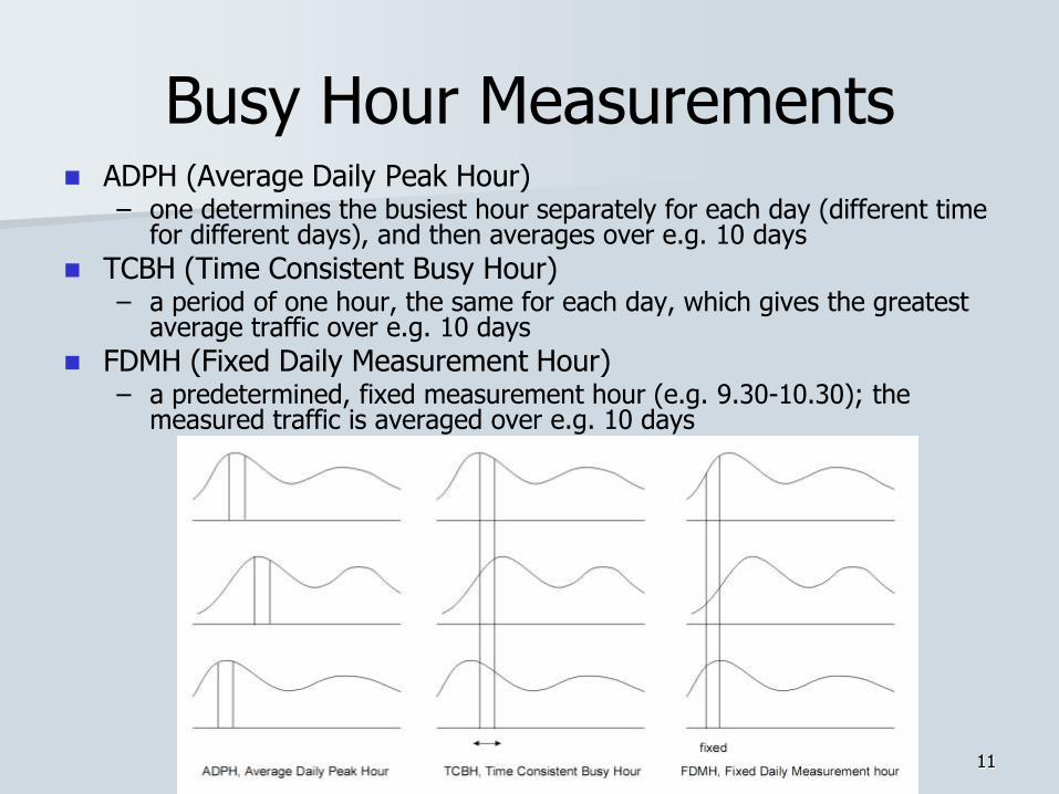
Busy Hour Measurements ADPH (Average Daily Peak Hour)
– one determines the busiest hour separately for each day (different time for different days), and then averages over e.g. 10 days
TCBH (Time Consistent Busy Hour) – a period of one hour, the same for each day, which gives the greatest
average traffic over e.g. 10 days
FDMH (Fixed Daily Measurement Hour) – a predetermined, fixed measurement hour (e.g. 9.30-10.30); the
measured traffic is averaged over e.g. 10 days
12
Traffic Model
Average arrival rate: λ(t) – depends on time, however it has a very strong deterministic component according to the profiles
In the busy hour period the average arrival time is considered stationary: λ, and the arrival process is considered as a Poisson process with intensity λ – Time homogenity
– Independence The future evolution of the process only depends upon the actual
state.
Independent of the user(!) – modeling all users in the same way
The average holding time (W(t)) is also considered to be stationary, and exponentially distributed with intensity μ
13 13
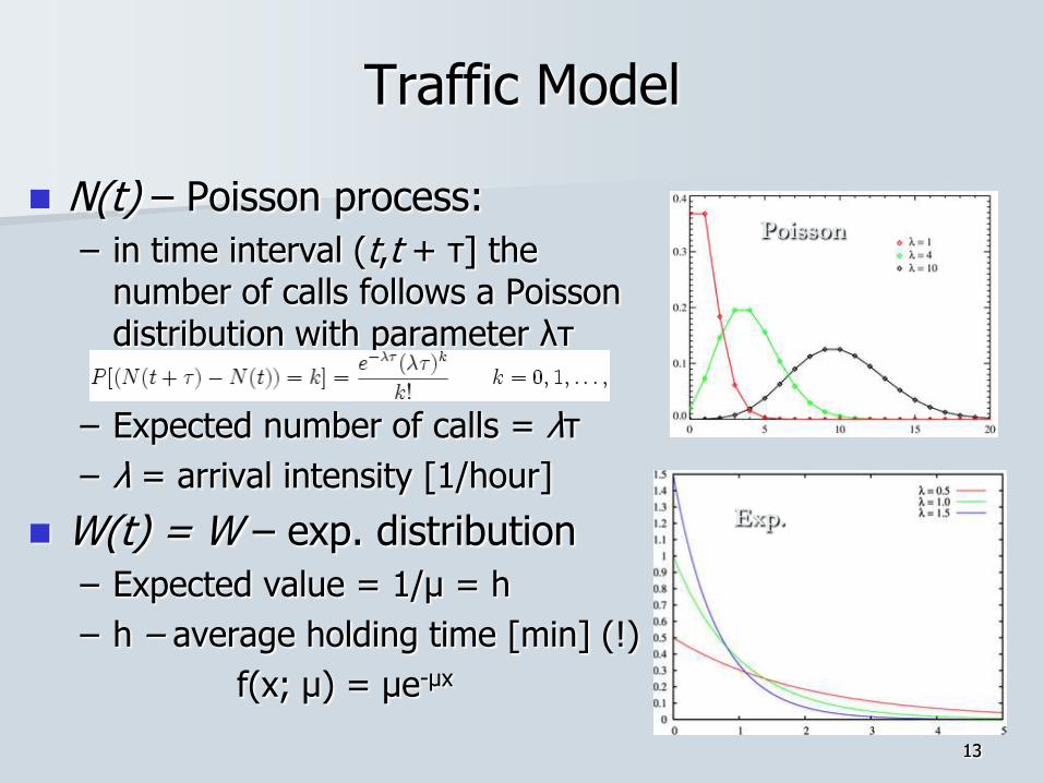
Traffic Model
N(t) – Poisson process:
– in time interval (t,t + τ] the number of calls follows a Poisson distribution with parameter λτ
– Expected number of calls = λτ
– λ = arrival intensity [1/hour]
W(t) = W – exp. distribution
– Expected value = 1/μ = h
– h – average holding time [min] (!)
f(x; μ) = μe-μx
Poisson
Exp.
14 14
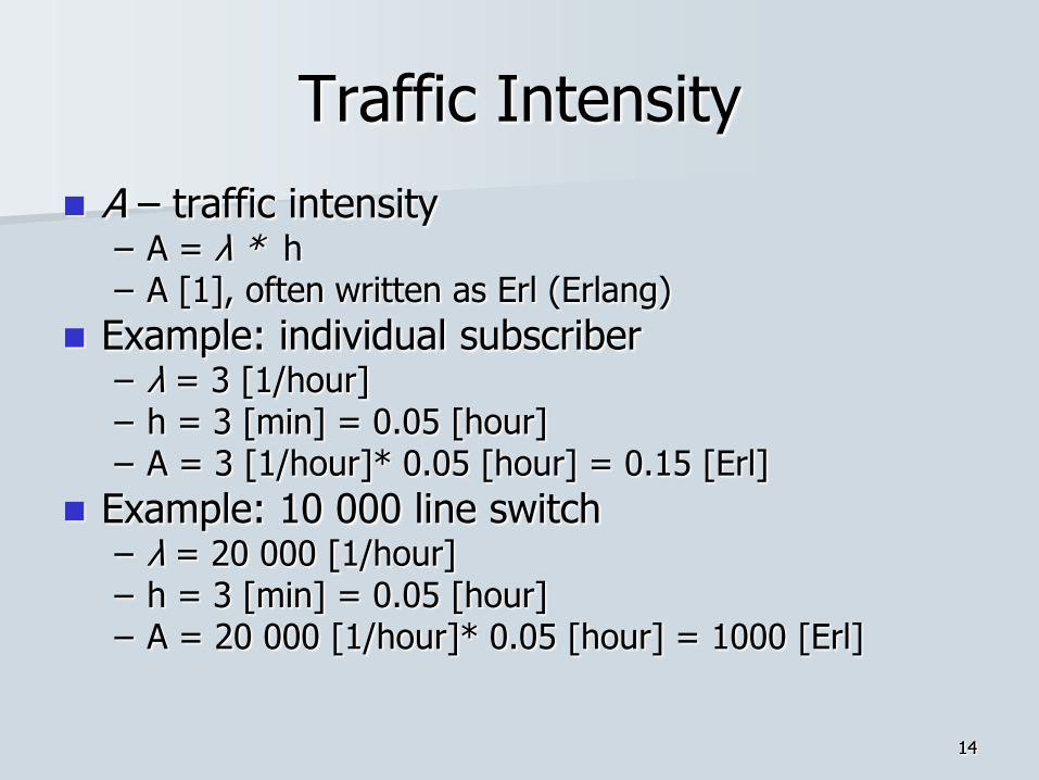
Traffic Intensity
A – traffic intensity – A = λ * h – A [1], often written as Erl (Erlang)
Example: individual subscriber – λ = 3 [1/hour] – h = 3 [min] = 0.05 [hour] – A = 3 [1/hour]* 0.05 [hour] = 0.15 [Erl]
Example: 10 000 line switch – λ = 20 000 [1/hour] – h = 3 [min] = 0.05 [hour] – A = 20 000 [1/hour]* 0.05 [hour] = 1000 [Erl]
15
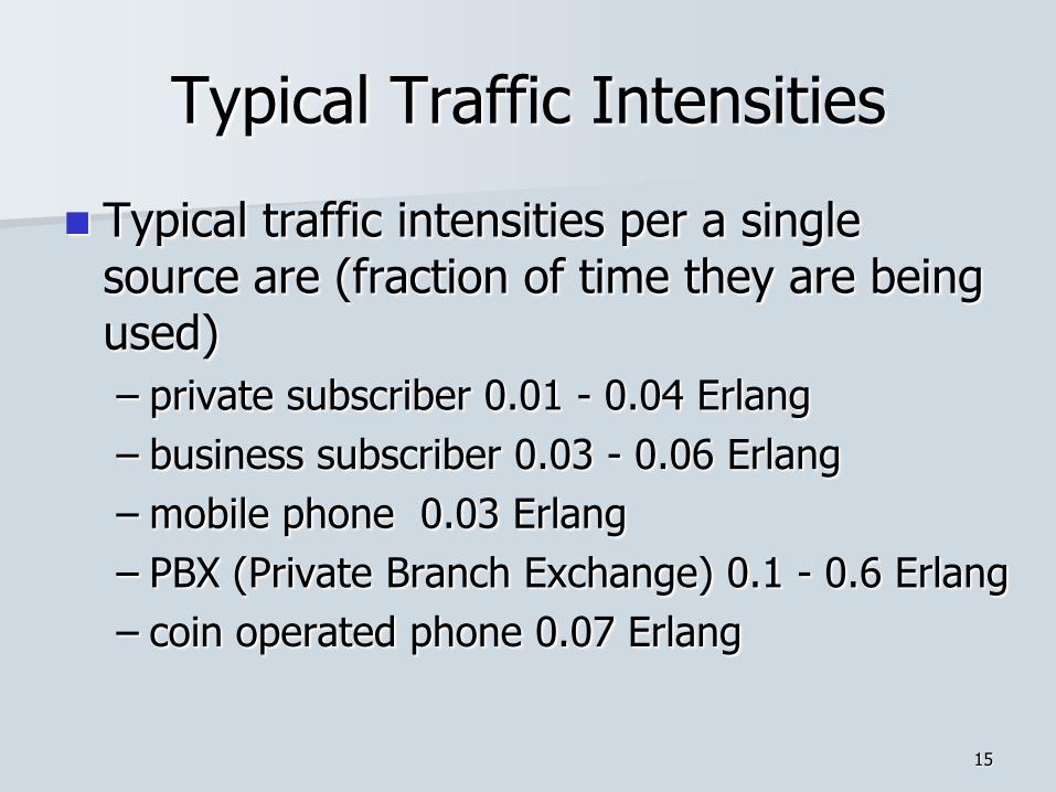
Typical Traffic Intensities
Typical traffic intensities per a single source are (fraction of time they are being used)
– private subscriber 0.01 - 0.04 Erlang
– business subscriber 0.03 - 0.06 Erlang
– mobile phone 0.03 Erlang
– PBX (Private Branch Exchange) 0.1 - 0.6 Erlang
– coin operated phone 0.07 Erlang
16
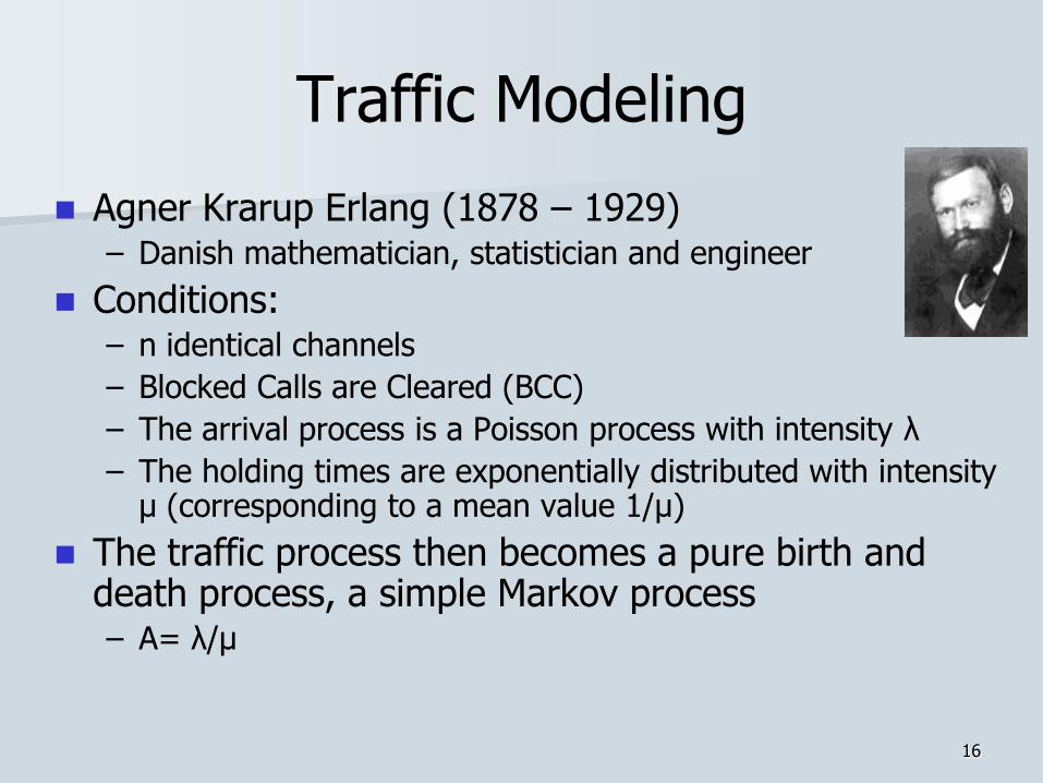
Traffic Modeling
Agner Krarup Erlang (1878 – 1929) – Danish mathematician, statistician and engineer
Conditions: – n identical channels
– Blocked Calls are Cleared (BCC)
– The arrival process is a Poisson process with intensity λ
– The holding times are exponentially distributed with intensity μ (corresponding to a mean value 1/μ)
The traffic process then becomes a pure birth and death process, a simple Markov process – A= λ/μ
17
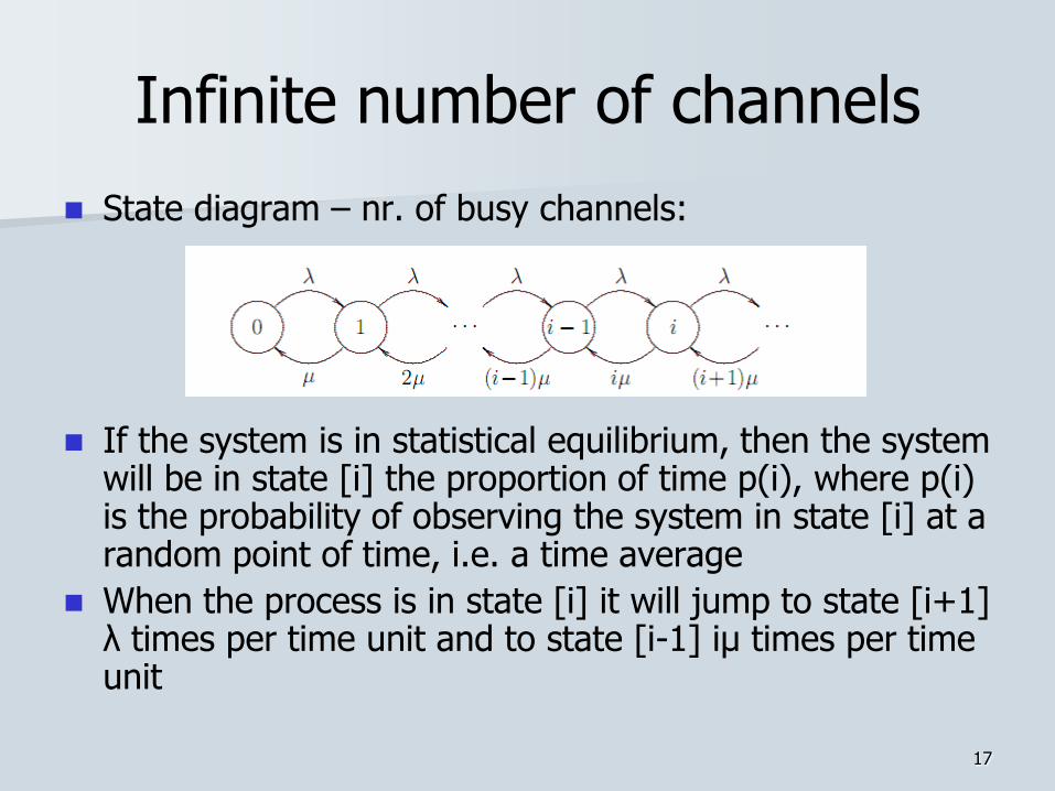
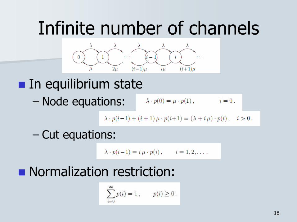
Infinite number of channels
State diagram – nr. of busy channels:
If the system is in statistical equilibrium, then the system will be in state [i] the proportion of time p(i), where p(i) is the probability of observing the system in state [i] at a random point of time, i.e. a time average
When the process is in state [i] it will jump to state [i+1] λ times per time unit and to state [i-1] iμ times per time unit
18
Infinite number of channels
In equilibrium state
– Node equations:
– Cut equations:
Normalization restriction:
19
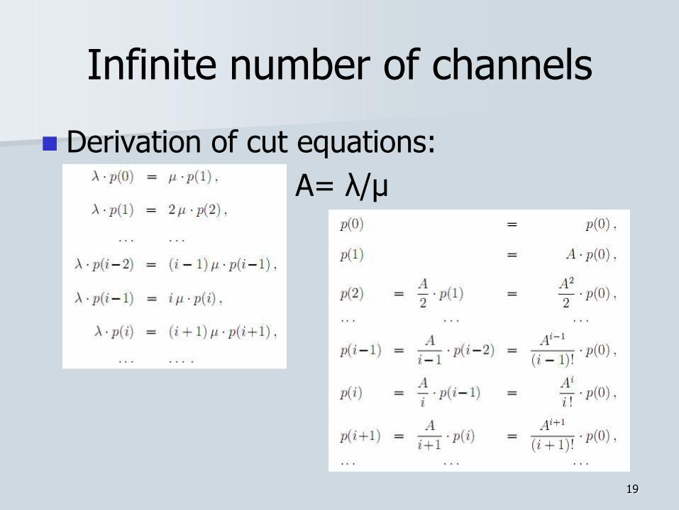
Infinite number of channels
Derivation of cut equations:
A= λ/μ
20
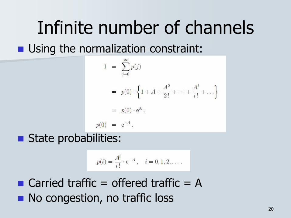
Infinite number of channels Using the normalization constraint:
State probabilities:
Carried traffic = offered traffic = A
No congestion, no traffic loss
21
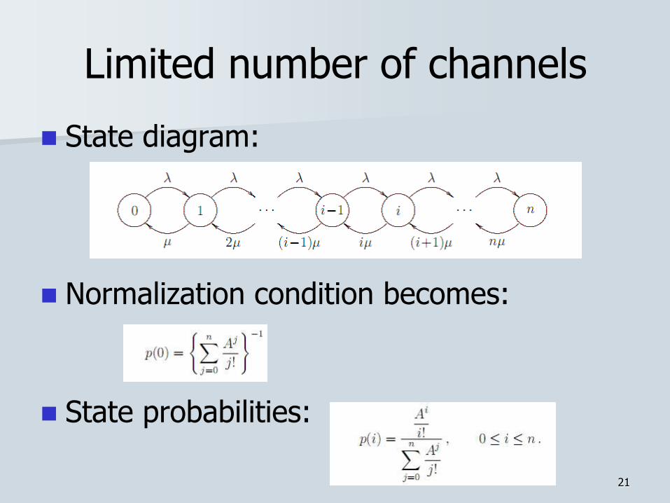
Limited number of channels
State diagram:
Normalization condition becomes:
State probabilities:
22
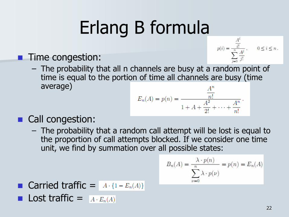
Erlang B formula
Time congestion: – The probability that all n channels are busy at a random point of
time is equal to the portion of time all channels are busy (time average)
Call congestion: – The probability that a random call attempt will be lost is equal to
the proportion of call attempts blocked. If we consider one time unit, we find by summation over all possible states:
Carried traffic =
Lost traffic =
23 23
Erlang B formula
Conditions for applicability:
– Gives good results if number of subscribers is much greater, than the number of channels (around 10x)
– Subscribers initiate calls independently from each other (not applicable e.g. if a TV advertisement presents a phone number and many people call it)
– The only reason for blocking is if all channels are busy
– Blocked Calls are Cleared, no waiting queue
– Subscribers do not repeat call attempt, if call was blocked
– The channel is occupied only by the particular subscribers, no resource sharing
24 24
Erlang B formula
25 25
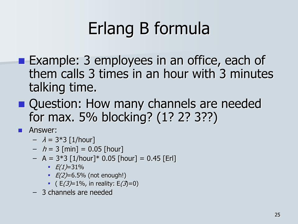
Erlang B formula
Example: 3 employees in an office, each of them calls 3 times in an hour with 3 minutes talking time.
Question: How many channels are needed for max. 5% blocking? (1? 2? 3??)
Answer: – λ = 3*3 [1/hour]
– h = 3 [min] = 0.05 [hour]
– A = 3*3 [1/hour]* 0.05 [hour] = 0.45 [Erl] E(1)=31%
E(2)=6.5% (not enough!)
( E(3)=1%, in reality: E(3)=0)
– 3 channels are needed
26 26
Erlang B formula
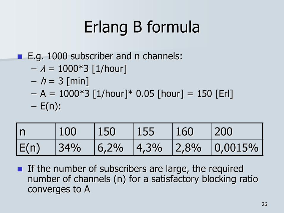
E.g. 1000 subscriber and n channels:
– λ = 1000*3 [1/hour]
– h = 3 [min]
– A = 1000*3 [1/hour]* 0.05 [hour] = 150 [Erl]
– E(n):
If the number of subscribers are large, the required number of channels (n) for a satisfactory blocking ratio converges to A
n 100 150 155 160 200
E(n) 34% 6,2% 4,3% 2,8% 0,0015%
27 27
Erlang B formula
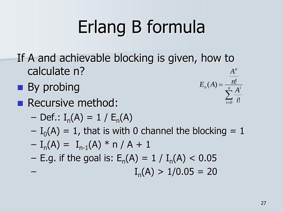
If A and achievable blocking is given, how to calculate n?
By probing
Recursive method:
– Def.: In(A) = 1 / En(A)
– I0(A) = 1, that is with 0 channel the blocking = 1
– In(A) = In-1(A) * n / A + 1
– E.g. if the goal is: En(A) = 1 / In(A) < 0.05
– In(A) > 1/0.05 = 20
n
i
i
n
n
i
A
n
A
AE
0 !
!)(

28
Extended Erlang B
Extended Erlang B: a certain percentage of blocked calls are reattempted – Iterative calculation with extra parameter, the Recall
Factor: Rf
– A0:initial traffic intensity
1. Calculate En(A0) with Erlang B
2. Nr. of blocked calls: B = A0 En(A0)
3. Nr. of recalls: R = Rf B
4. New offered traffic: A1 = A0+ R
5. Return to step 1 and iterate until value of A is stabilized
29
Erlang C formula
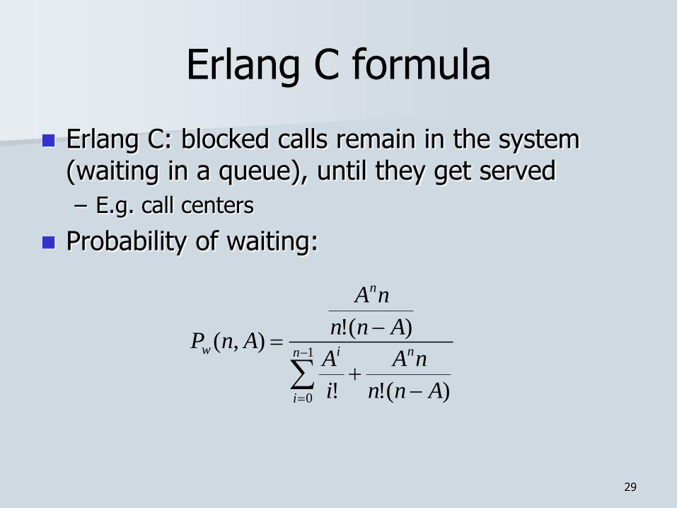
Erlang C: blocked calls remain in the system (waiting in a queue), until they get served
– E.g. call centers
Probability of waiting:
1
0 )(!!
)(!),(
n
i
ni
n
w
Ann
nA
i
A
Ann
nA
AnP

Exercises
30
31
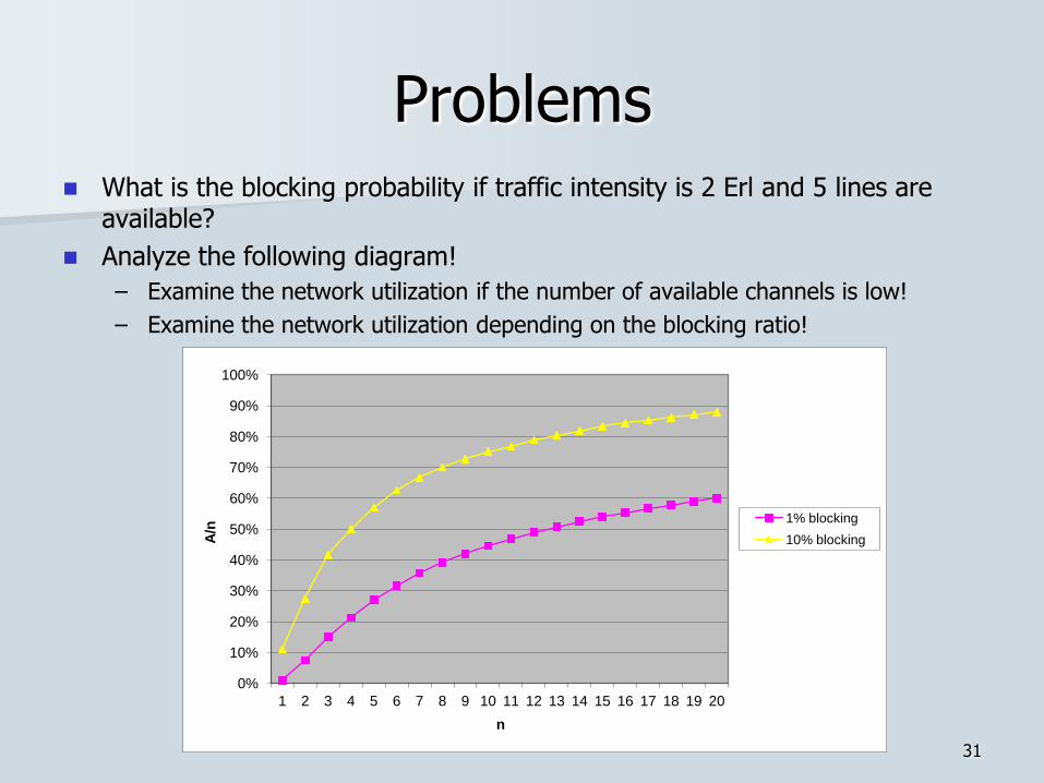
Problems What is the blocking probability if traffic intensity is 2 Erl and 5 lines are
available?
Analyze the following diagram!
– Examine the network utilization if the number of available channels is low!
– Examine the network utilization depending on the blocking ratio!
0%
10%
20%
30%
40%
50%
60%
70%
80%
90%
100%
1 2 3 4 5 6 7 8 9 10 11 12 13 14 15 16 17 18 19 20
A/n
n
1% blocking
10% blocking

32
Problems
How many lines are required for 100 subscribers, when they individually generate 0.04 Erl traffic intensity? – if the allowed blocking ratio is 20%?
– if the allowed blocking ratio is 1%?
20 employees work in an office with 2 lines. What is the blocking ratio if employees call with 0.1 Erl intensity?
33
Problems
10 employees work in an office with 3 lines. What is the blocking ratio if employees initiate once a 15 min long call in the busy hour?
– Average utilization of lines? – Blocking ratio? – Is it a well dimensioned system?
A subscriber generates 0.1 Erl traffic intensity. How many lines are required, if the blocking requirement is 1% and the number of subscribers are – 10? (5) – 100? (18) – 1 000? (117) – 4 000? (426) – 10 000? (1029)


