
Breaking the misconceptions: An analysis of the effects financial
liberalization on financial development using index measures
This paper examines the link between financial openness and financial development through a panel
data analysis on advanced and emerging market countries. Using index measures for financial openness
and financial development, we show that financial openness together with institutional, educational and
macroeconomic variables can explain a large part of the variation in financial development across
countries and over time. Our analysis shows that different kind of indexing strategies could aid in
finding a better measure for financial openness and financial development. Additional robustness checks
and the endogeneity analysis reveal that the findings are robust to different lag structures, time
dummies, trends, and reductions in the sample size. Financial openness is found to have a positive effect
on financial development independent from the lag structure chosen, and time dummies and trends
used. The positive influence of financial openness carries out even when the sample size is reduced to
developing countries.
Zeynep Özkök
Supervised by: Dr. Klaus Desmet
2
Breaking the misconceptions: An analysis of the effects financial liberalization
on financial development using index measures
Table of Contents
1. Introduction ....................................................................................................................................... 3
2. The Data ............................................................................................................................................. 6
2.1. Individual Measures ....................................................................................................................... 6
2.2 Aggregate Index Measures ............................................................................................................ 11
3. Empirical Model .............................................................................................................................. 17
4. Empirical Results ............................................................................................................................. 22
4.1 Results using equally weighted index measures ............................................................................. 23
4.2 Results using coefficient of variation type index measures ............................................................. 24
4.3 Results using principal component analysis type index measures ................................................... 25
4.4 Adding the interaction term .......................................................................................................... 28
5. Robustness checks and further issues ............................................................................................ 30
5.1 Robustness checks ........................................................................................................................ 30
5.2 Further issues ............................................................................................................................... 32
6. Concluding remarks ......................................................................................................................... 34
References ........................................................................................................................................... 35
Appendix .............................................................................................................................................. 41
Additional Web Appendices ............................................................................................................... 74
Data Appendix ................................................................................................................................... 74
Supplementary Appendix ................................................................................................................... 78
3
1. Introduction
In the wake of the recent financial crisis, the role of financial development in emerging markets and
developed countries has become a source of interest to many researchers. Financial development,
defined generally as the channel for increasing the efficiency of financial markets and resources,
monitoring investment projects, and the banking sector and improving on the overall importance of the
financial system, is viewed as a major element influencing economic growth and welfare.1
As the role of financial development on economic growth is recognized, there has become a wide spread
debate on the effects of financial liberalization on growth and financial development. Financial
liberalization described as the alleviation of capital controls, allowance of capital flows within and across
countries, deregulation of domestic financial markets and liberalization of capital accounts should
reduce macroeconomic volatility and thereby help promote financial sector development. Studies have
shown that financial liberalization can endorse economic growth and enhance welfare through
opportunities for a better and more efficient allocation of resources, through portfolio and risk
diversification and higher profitability of investment given that there exist appropriate controls,
frameworks and regulatory apparatus.2 3
Although the literature provides a broad examination of financial liberalization and economic growth,
the link between financial liberalization and financial development has been overlooked. We believe
that a proper analysis of this link will help clarify the ambiguity in the relationship between financial
liberalization and economic growth.
The small strand of literature generally attempts to answer the question regarding the effects of trade
and capital account openness on financial development and analyzes the possible influence of economic
institutions, legal and country specific variables, and educational attainment measures on financial
development. Various authors from Chinn and Ito (2002) and (2006), Ito (2006), Baltagi, Demetriades
and Law (2007), Demetriades and Law (2006), Demetriades and Andrianova (2005) and Huang (2007)
examine the effect of capital account liberalization on the development of equity markets controlling for
legal systems and institutions among mostly developed and emerging market economies. The results of
the panel data analysis by and large demonstrate that financial liberalization (capital account openness
in most cases) contributes to financial development in equity and stock markets for both less developed
and emerging market countries. The results also show that opening up capital accounts can be beneficial
for financial development only if the country under examination has attained a threshold level of legal
and institutional development.4 Trade openness and banking sector development are found to be
preconditions for financial openness and financial development in most studies.
1 Huang, Wei, “Emerging Markets, Financial Openness, and Financial Development”, University of Bristol Discussion
Paper, 2006 – 588, pp. 2 2 Aziakpono, Jesse Meshach, “Effects of Financial Integration on Financial Development and Economic Performance
of the SACU countries”, Paper presented at the ECA/ADB African Economic Conferences, (2007), pp. 2 3 Ibid., pp. 2
4 Ibid., pp. 12
4
The literature shows that there are three main issues in examining the relationship between financial
liberalization and financial development. First, the choice of indicators has been a topic of concern. One
needs a broad indicator that can incorporate different aspects of various measures suggested for
financial liberalization. Studies lack a comprehensive indicator that can bring together all features of
financial development such as the banking system, the stock and bond markets. With different
measures used for financial openness, the most prominent measure of financial liberalization, and for
financial development the results obtained seem unconvincing. Another concern with different
measures is that the results from various studies become hardly comparable due to particular choice of
individual measures used by the authors and the country and time coverage selected for the study.
Building better financial openness and financial development indices will help resolve problems
associated with particular choice of measures. Second, the number of countries included in most studies
is limited. Due to the lack of data for many less developed and some emerging market countries, most
economists use developed countries in their estimations, which highly influence the results. Third, what
seems to be a minor issue, which in reality can affect almost all findings, is the choice of control
variables. The literature shows that the choice of the control variables can influence the link between
financial openness and financial development. The correct specification of control variables can lead to a
better examination of these concepts.
The issues regarding the measurement and the choice of financial openness, financial development and
control variables thereby remain to be thoroughly explored. The essential point, however, is to explore
whether differences in terms of absorbing the benefits of financial liberalization among countries result
due to the ability of countries through different institutions, policies and regulations to convert financial
openness into financial development. One can argue that if financial openness can lead to the
development of a stable financial system, alongside well-functioning financial markets, this process can
then bring about an increase in the welfare of the society which can even enhance economic growth.
The question of the necessity of financial liberalization to translate into financial development so as to
achieve economic growth and welfare remains to be at the core of this study.
This paper, by this means, aims to examine the link between financial openness and financial
development through a panel study of developed and emerging market countries. Using index
measures we show that financial openness together with institutional, educational and macroeconomic
variables can explain a large part of the variation in financial development across countries and over
time. Principal component type index measures provide better results in terms of economic and
statistical significances. The results after the inclusion of the interaction term show that there is a
negative relationship between financial development and the simultaneous opening of financial and
goods markets. The robustness checks and the endogeneity analysis show that the findings are robust to
different lag structures, time dummies, trends, and reductions in the sample size.
We add to the literature on three aspects. First, we give a comparative view on different index measures
for financial openness and financial development straining away from choosing individual variables
which we believe do not fully represent the aspects of financial openness and financial development.
Second, we examine the simultaneity hypothesis of opening financial and goods markets with index
measures. Lastly we explicitly study one of the main problems of panel data models; endogeneity issues.

5
Our paper, to our knowledge, is the first one to compare different index measures for financial openness
and financial development with the hope of identifying the relationship among the two. We
complement Huang’s (2006) work by suggesting additional principal components type indices for
financial openness and financial development and by offering a broad comparison among the different
types of indices used in the analysis.
This paper is organized as follows. Section 2 introduces the data used in the analysis and briefly
describes the aggregate indices of financial openness and financial development. Section 3 explains the
empirical model and emphasizes on the estimation procedure. Section 4 reports the estimation results.
Section 5 discusses the robustness checks and further issues related to our sample. Section 6 concludes
by summarizing our findings.
6
2. The Data
This section introduces the variables used as measures of financial openness and financial development.
We first discuss the individual indicators and then construct aggregate index measures with different
groups of these measures.
One main problem in obtaining financial data for numerous countries is the tradeoff between having a
large estimation period and a wide number of countries. As the estimation period for the panel data
enlarges the number of countries for which the indicators of financial openness and financial
development are available reduces. In order to avoid this difficulty we choose 61 countries for which we
have data over the 1970 – 2007 period. However, for the main analysis we use a subgroup of the data,
1996 – 2007 period, in order to avoid as many missing values as possible.
The analysis is based on annual data obtained primarily from Beck, Demirguc-Kunt, and Levine’s
database (referred as BDL from onwards), the World Bank’s World Development Indicators (WDI), World
Governance Indicators, Edstats which extracts data from the UNESCO Institute for Statistics, and the
IMF’s International Financial Statistics. We, hereby, summarize the individual and aggregate measures
for financial openness and financial development along with the control variables used in our analysis.
2.1 Individual Measures
2.1.1 Financial Openness Indicators
Financial openness is measured with market capitalization of listed companies (% of GDP), foreign direct
investment (% of GDP), number of domestic companies listed (per million population), portfolio
investment flows (% of GDP), and international debt issues (% of GDP).
Our first measure of financial openness, market capitalization of listed companies (% of GDP), is equal
to the value of listed shares divided by GDP and is regarded as a measure of the size of stock markets
relative to the economy.5 It is most frequently used as a measurement of the corporate size of
companies. The second measure, foreign direct investment, is the sum of net inflows and outflows of
foreign direct investment recorded as a percentage of GDP. This indicator adds up equity capital,
reinvestment of earnings and other short- and long-term capital.6
The third financial openness indicator is the number of domestic companies listed per million population.
The World Bank defines this variable as the domestically incorporated companies listed on the country’s
stock exchanges at the end of the year.7 This indicator is another measure of market size. The fourth
measure of financial openness, portfolio investment flows (% of GDP), is the sum of portfolio debt flows
(private and publicly guaranteed and private nonguaranteed bond issues purchased by foreign
5 Demirguc-Kunt, Asli, and Ross Levine, Financial Structure and Economic Growth: A Cross-Country Comparison of
Banks, Markets, and Development, MIT Press, 2001, pp. 195 6 World Bank, 2007 World Development Indicators, International Bank for Reconstruction and Development/The
World Bank Press, 2007, pp. 319 7 Ibid., pp. 279
7
investors) and non-debt-creating portfolio equity flows which are equal to the sum of country funds,
depository receipts, and direct purchases of shares by foreign investors.8 Portfolio investment
constitutes one of the main elements of capital flows and we believe that the inclusion of this variable
will help determine the role played by portfolio investment across countries.
The fifth and last measure of financial openness is international debt issues (% of GDP) introduced by
BDL in their latest database. International debt flows measures “the net flow of international bond
issues relative to a country’s economic activity”.9
The literature suggests the use of market capitalization of companies, gross foreign direct investment,
gross private capital flows, and some independent indices as measures of financial openness. Among
these indicators we employ the market capitalization of companies and foreign direct investment as our
prospective measures of financial openness. Gross private capital flows are excluded from our analysis
and are replaced by portfolio investment flows due to their discontinuity by the World Bank. Portfolio
investment flows, which were one of the main determinants of private capital flows, are utilized to
highlight the importance of portfolio investment across countries. Different from the literature we also
make use of indicators such as the number of domestic companies listed per million population and
international debt issues. We believe that the inclusion of both of these variables as measures of
financial openness will be essential in determining the optimal estimator of financial openness.
As summarized by Kose et.al (200.) financial openness indicators are divided into two mainstream
measures; de jure measures which depend on the removal of legal restrictions on cross-border capital
flows, and the removal of controls on prices, quantities and foreign equity holdings and de facto
measures which observe countries’ integrations into the world capital and financial markets in all
practical terms.10 De jure measures are typically based on IMF indicators such as the Annual Report on
Exchange Arrangements and Exchange Restrictions (AREAER) and illustrate the number of years for
which a country’s capital accounts have been open and free from restrictions and controls. The AREAER
measure along with Chinn and Ito’s (2005) principal component based financial openness measure,
Quinn’s capital account openness index (1997, 2003), Mody and Murshid’s (2005) and Edwards’s (2005)
measures on capital and current account restrictions are mostly based on narrative and discrete 0-1
type variables, “indicating full openness or closedness”.11 De jure measures have long been accused of
not being able to fully reflect the degree of financial or capital account openness due to their reliance on
the removal of restrictions associated with foreign exchange transactions.12 Even though these
measures rely on the elimination of controls and restrictions on capital account they do not particularly
capture “the degree of enforcement or the effectiveness of enforcement” of these restrictions.13
8 Ibid., pp. 343
9 Beck, Thorsten, and Asli Demirguc-Kunt, “Financial Institutions and Markets Across Countries and Over Time –
Data and Analysis”, World Bank Working Paper, (2009), pp. 15 10
Kose, Ayhan, Eswar Prasad, Kenneth Rogoff, and Shang-Jin Wei, “Financial globalization: a reappraisal”, NBER Working Paper No. 12484, (2006), pp. 12 11
Ibid., pp. 11 12
Ibid., pp. 13 13
Ibid., pp. 13

8
Despite the fact that these types of indices are developed to measure financial globalization in terms of
openness of capital and financial markets, they do not represent the degree of integration into the
global markets. Alternatively, de facto measures which are grouped into price differential and quantity
based indicators examine the applied side by taking into account both legal restrictions and capital
flows. However, due to the difficulty in interpreting and utilizing price differential based de facto
measures, quantity based indicators of financial openness are more frequently used. Although the
quantity based de facto measures such as gross capital flows, may bring measurement errors and may
create difficulty in overcoming endogenity and causality issues, they remain to be the superior measure
of financial integration.14 For all the above reasons, we restrain from using discrete de jure measures
and prefer to use stock and flow variables to measure financial openness. We believe that through the
use of de facto openness indicators we will be able to examine the full aspect of financial and capital
markets in all practical terms.
2.1.2 Financial Development Indicators
Due to a wide range of financial development indicators used in this analysis we group the data into
several different categories. We consider that the combination of these categories will help determine
the aggregate effect of financial openness on financial development.
a) Banking sector development indicators:
We use six indicators to measure the development of the banking sector. These variables are liquid
liabilities (% of GDP), private credit by deposit money banks and other financial institutions (% of GDP),
the ratio of deposit money bank assets to the sum of deposit money bank assets and central bank assets
(in percentages), total bank assets (% of GDP), deposit money bank assets to central bank assets ratio (in
percentages), and domestic credit provided by the banking sector (% of GDP). All data used for this
category is available from the Financial Structure database by BDL and the World Bank’s WDI. The data
specified is annual and can be obtained online.
Liquid liabilities (% of GDP) equals the ratio of liquid liabilities of bank and nonbank financial
intermediaries to GDP.15 This variable is commonly used as an overall measure of financial sector
development and a typical measure of financial depth.
Private credit by deposit money banks and other institutions (% of GDP) is an indicator for the overall
development in private banking markets.16 This variable refers to financial resources provided to the
private sector by deposit money banks and other financial institutions and it solely measures the credit
provided to the private sector.
14
Ibid., pp. 14 15
Demirguc-Kunt, Asli, and Ross Levine, Financial Structure and Economic Growth: A Cross-Country Comparison of Banks, Markets, and Development, MIT Press, 2001, pp. 84 16
Chinn, Menzie, and Hiro Ito, “What matters for financial development? Capital controls, institutions, and interactions”, Journal of Development Economics, (2006), pp. 5

9
The ratio of deposit money bank assets to the sum of deposit money bank assets and central bank assets
(in percentages) is used to show the weight of deposit money bank assets among total assets. It reflects
the importance of private lending compared to total lending.17
Deposit money bank assets to central bank assets ratio (in percentages) highlights the importance of
private lending to government lending.18
Total bank assets (% of GDP) is used as a measure of financial depth. It is used to represent the overall
size of the banking sector.
Domestic credit provided by the banking sector (% of GDP) includes credit extended to the private sector
and general government, to the nonfinancial public sector in the form of investments in short- and long-
term government securities, to banking and nonbank institutions and loans to state enterprises but
excludes credit to the central government.19 This indicator is a measure of banking sector depth and
financial sector development in terms of size.20
The variables used to determine the banking sector development indicators correspond to the ones
used in the literature. We believe that a wide range of different variables will help us capture all possible
aspects of banking sector development. We include a broader selection of variables here in order to
fully capture the importance of the banking sector on overall financial development.
b) Stock market development indicators:
We use three different variables to measure development in stock markets. These three variables are
stock market capitalization (% of GDP), stock market turnover ratio (in percentages), and stock market
total value traded (% of GDP). The data listed below is annual and is extracted from the Financial
Structure database of BDL.
Stock market capitalization (% of GDP) is equal to the value of listed shares divided by GDP. It is an
indicator of the size of the stock market. Stock market turnover ratio (in percentages) is used as the
efficiency indicator of stock markets.21 It is classified as the ratio of the value of total shares traded to
stock market capitalization. Stock market total value traded (% of GDP) is equal to the total shares
traded on the stock market exchange divided by GDP. This indicator measures the activity or liquidity of
the stock markets.22
17
Huang, Wei, “Emerging Markets, Financial Openness, and Financial Development”, University of Bristol Discussion Paper, 2006 – 588, pp. 10 18
Ibid., pp. 10 19
World Bank, 2007 World Development Indicators, International Bank for Reconstruction and Development/The World Bank Press, 2007, pp. 241 20
Ibid., pp. 283 21
Demirguc-Kunt, Asli, and Ross Levine, Financial Structure and Economic Growth: A Cross-Country Comparison of Banks, Markets, and Development, MIT Press, 2001, pp. 32 22
Ibid., pp. 32
10
Stock market development indicators used also correspond to the ones found in the literature. The
three indicators are the most frequently used indicators to measure stock market development and we
believe that they will summarize all prospects of stock market development.
c) Bond market development indicators:
Private bond market capitalization (% of GDP) and public bond market capitalization (% of GDP) are the
two indicators used to measure bond market development. Data is reported annually from the Financial
Structure database of BDL.
Private bond market capitalization (% of GDP) is equal to the total amount of outstanding domestic debt
securities issued by financial institutions and corporations as a share of GDP. Public bond market
capitalization (% of GDP) on the other hand is equal to the total amount of public domestic securities
issued by governments as a share of GDP. Both of these indicators are used to determine the efficiency
of bond markets.
Bond market development indicators have not been used in the literature on financial openness and
financial development. Even though these indicators have been employed excessively in equity market
development literature, due to the short period of data availability they have not been used as
indicators for financial development. Since we consider a sub period in our analysis in order to obtain a
broader perspective of the effects of financial openness on financial development we propose using the
bond market development indicators so as to capture the efficiency and the effectiveness of bond
markets on the overall level of financial development.
2.1.3 Control Variables
In order to examine the effect of financial openness on financial development we introduce a broad
range of control variables. These variables allow us to analyze the true impact of financial openness on
financial development as we control for possible influential effects. The control variables used in this
paper include GDP per capita, GDP growth, trade openness, secondary school enrollment rate, and legal
and institutional variables. The data is available from the World Bank’s WDI and the World Governance
Indicators, and Edstats databases by the World Bank.
Logarithm of GDP per capita (in constant 2000 US dollars) and GDP growth (in annual percentages) are
used as measures for economic performance among countries. We employ these measures to control
for the demand of finance and to monitor the differences in performances and productivities across
countries.
Trade openness (% of GDP) measured by the sum of imports and exports of goods and services is used to
determine whether trade liberalization is a precondition for financial liberalization. Controlling for trade
openness allows examining the direct effects of financial liberalization on financial development.
Secondary school gross enrolment rate (% of population) is used as an indicator that controls for
differences in educational attainment across countries. We consider this measure as an important
reason for why we observe disparities across countries in their levels of financial development. Even

11
though there has not been a study that utilizes an educational attainment indicator as a control variable
in the financial openness and financial development literature, we believe that the inclusion of such a
variable can also alter our findings. If the wide educational gaps that are observed between developed,
emerging market and less developed countries affect the link between financial openness and financial
development then the exclusion of such a variable would certainly introduce a measurement bias.
Following the examples of educational attainment indicators used in the economic growth literature we
take secondary school gross enrollment rate as a possible determinant for why we examine differences
across countries in terms of grasping the benefits of financial liberalization.
Lastly legal and institutional variables are used to measure the economic institutions and the overall
quality of legal systems. We employ four different measures to control for institutional, legal, political
and economic factors that may affect the overall level of financial development. These indicators are
based on both subjective and perceptions-based data that reflect views of a range of respondents,
agencies and organizations. They are constructed as a first tool for cross-country comparisons, and
examination of ongoing trends over time.23 These indicators are government effectiveness, regulatory
quality, rule of law, and control corruption and they are measured through a range from-2.5 to 2.5
where higher values correspond to better governance outcomes.24 Following Baltagi, Demetriades and
Law (2007), Huang (2006) and Chinn and Ito (2005), we use institutional and legal variables to determine
their influence on the relationship between financial openness and financial development. Differently
from the authors mentioned we employ four different measures from the World Governance Indicators
due to better data availability and greater country coverage.
The institutional quality variables used in our analysis are time-invariant. Given that our analysis is
based on panel data specifications that can show variations across time, the use of time-invariant
control variables may constitute a main drawback. However, as Chinn and Ito (2005) explain, the
inclusion of these time-invariant factors do not pose a substantial problem for our analysis since the
characteristics given by institutional quality variables are likely to change very slowly.25 On this note, due
to the time invariability of these indicators, we take the averages of two consecutive years to replace
the missing years’ data in the World Governance Indicators database for the four legal/institutional
quality variables.
2.2 Aggregate Index Measures
Aggregating different measures of financial openness and financial development into a single index aids
in summarizing the comprehensive nature of the financial sector.
23
Daniel Kaufmann, Aart Kraay and Massimo Mastruzzi, “Governance Matters VIII: Governance Indicators for 1996-2008”, World Bank Policy Research, (2009), pp. 7 24
World Governance Indicators (WGI) dataset, World Bank, http://info.worldbank.org/governance/wgi/index.asp 25
Chinn, Menzie, and Hiro Ito, “What matters for financial development? Capital controls, institutions, and interactions”, Journal of Development Economics, (2005), pp. 10

12
2.2.1 Equally weighted index measure
We first construct equally weighted indicators for financial openness, banking sector, bond and stock
market, and overall financial development as well as for institutional quality. Our final equally weighted
indicators are averages of the banking sector, bond and stock market, and financial development
indicators. The biggest problem with equally weighted indicators is that different measures of financial
openness and financial development may have different weights and equally weighted indicators may
over-or-underestimate the importance of such measures. This could potentially bias our results. In
order to avoid this possibility we construct indices using other approaches.
2.2.2 Coefficient of variation type index measure
The second methodology followed in constructing indices uses the coefficient of variation approach.26
The weights for the indices for financial openness, financial development, and institutional quality are
calculated using the coefficient of variation for each variable and the sum of all coefficients of variation
for all the variables to be used in the index. The weights following this method will be constructed as
follows:
where is the sum of all coefficients of variations for the given number of variables, and denotes
the coefficient of variation of each variable and can be found by:
where and are the mean and standard deviation of these residuals respectively.
This procedure, thereby, allows for weighing each variable differently in the financial openness, financial
development and institutional quality indices. It helps avoid the potential bias that may occur when
using equal weights as described previously.
We can then construct indices for financial openness, financial development, and institutional quality as:
where is the relative weight of each variable in the financial openness index and denotes each
of the measures used for constructing the financial openness index. is market capitalization of
26
For more information please refer to: Ullah, Aman, and Davide E. A Giles, Handbook of Applied Economic Statistics, Marcel Dekker, Inc., N.Y. 1998, and Sheret, Michael, “The Coefficient of Variation: Weighting Considerations”, Social Indicators Research, (1984), Vol. 15, No. 3

13
listed companies (% of GDP), foreign direct investment (% of GDP), listed domestic companies (per
million population), international debt issues (% of GDP) and portfolio investment flows (% of GDP)
respectively.
Similarly, banking sector, bond and stock market and financial development, and institutional quality
indices are constructed as weighted averages of the corresponding variables as described previously.
2.2.3 Principal Component Analysis for an index measure
The third methodology used in constructing index measures is the principal component analysis.
Principal components analysis in its simplest form involves a mathematical procedure that helps
transform a number of possibly correlated variables into a smaller number of uncorrelated ones which
we call principal components. This type of analysis has two main objectives; reducing the dimensionality
of the data set, and identifying new meaningful variables.27
Our dataset contains a large number of variables which summarize the information for both financial
openness and financial development. Principal component analysis here aids in determining the weights
of the variables to be included in an index arbitrarily by constructing in such a way that “the resulting
components account for a maximal amount of variance in the data set”.28 This method has been shown
to be more efficient in establishing the optimal weights of variables in comparison to other type of
methods where variables are given equal or subjective weights according to the method employed.
The theory behind the principal components analysis is as follows:
Suppose that y1 is a principal component of x1,x2, x3, …, xp, such that:
Then the variance of y1 is maximized given the constraint that the sum of the squared weights of x1,x2,
x3, …,xp is equal to one.29 That is:
The random variables, xi can be standardized scores or deviations from the mean scores.30 Using
principal component analysis we can find the optimal weight vector (a11, a12, … ,a1p ) and the associated
27
http://www.fon.hum.uva.nl/praat/manual/Principal_component_analysis.html 28
Principal component analysis, pp. 7, http://support.sas.com/publishing/pubcat/chaps/55129.pdf 29
Ibid., pp. 11 30
A score is “a linear composite of the optimally-weighted observed variables”. We use standardized scores or deviations of the observed variables from their means in order to obtain observations with zero mean and unit variance in each column. Principal component analysis, pp. 11, http://support.sas.com/publishing/pubcat/chaps/55129.pdf
14
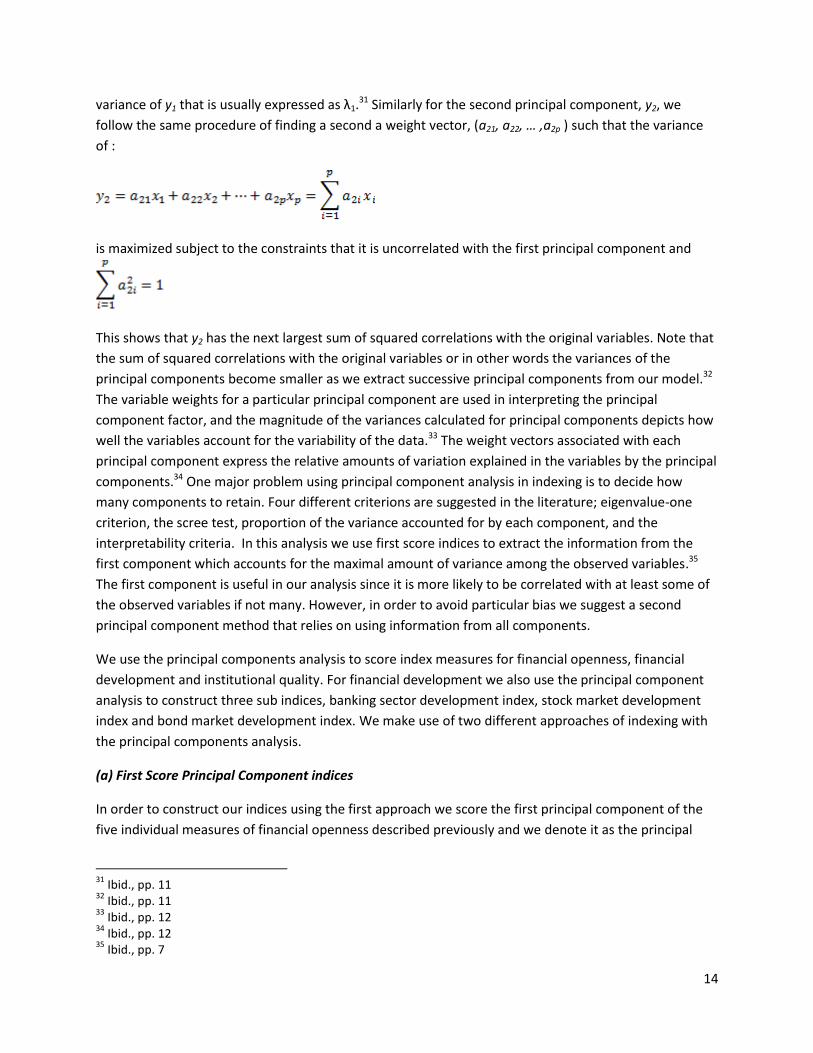
variance of y1 that is usually expressed as λ1.31 Similarly for the second principal component, y2, we
follow the same procedure of finding a second a weight vector, (a21, a22, … ,a2p ) such that the variance
of :
is maximized subject to the constraints that it is uncorrelated with the first principal component and
This shows that y2 has the next largest sum of squared correlations with the original variables. Note that
the sum of squared correlations with the original variables or in other words the variances of the
principal components become smaller as we extract successive principal components from our model.32
The variable weights for a particular principal component are used in interpreting the principal
component factor, and the magnitude of the variances calculated for principal components depicts how
well the variables account for the variability of the data.33 The weight vectors associated with each
principal component express the relative amounts of variation explained in the variables by the principal
components.34 One major problem using principal component analysis in indexing is to decide how
many components to retain. Four different criterions are suggested in the literature; eigenvalue-one
criterion, the scree test, proportion of the variance accounted for by each component, and the
interpretability criteria. In this analysis we use first score indices to extract the information from the
first component which accounts for the maximal amount of variance among the observed variables.35
The first component is useful in our analysis since it is more likely to be correlated with at least some of
the observed variables if not many. However, in order to avoid particular bias we suggest a second
principal component method that relies on using information from all components.
We use the principal components analysis to score index measures for financial openness, financial
development and institutional quality. For financial development we also use the principal component
analysis to construct three sub indices, banking sector development index, stock market development
index and bond market development index. We make use of two different approaches of indexing with
the principal components analysis.
(a) First Score Principal Component indices
In order to construct our indices using the first approach we score the first principal component of the
five individual measures of financial openness described previously and we denote it as the principal
31
Ibid., pp. 11 32
Ibid., pp. 11 33
Ibid., pp. 12 34
Ibid., pp. 12 35
Ibid., pp. 7
15
component index measure of financial openness, PCFO. Similarly the index measures of financial
development, PCFD, will be determined by the first principal component of the combination of three
different development indicators, a total of 11 variables. Excluding deposit money bank assets to central
bank assets ratio from our analysis, we also construct another financial development index with 10
variables, PCFD4. We construct first principal component indices for banking sector development, PCBD,
stock market development, PCSMD, and bond market development, PCBMD. Institutional quality index,
PCINSQUA, is constructed using the first score of the four variables that compromise this index.
(b) Principal Components analysis type indices that take into account information in all components
In order to ensure whether our first score principal component type indices are underestimating the
strength of the link between financial openness and financial development we utilize an additional
principal component indexing strategy to take into account all possible components so as not to discard
any information that could potentially affect our estimations.
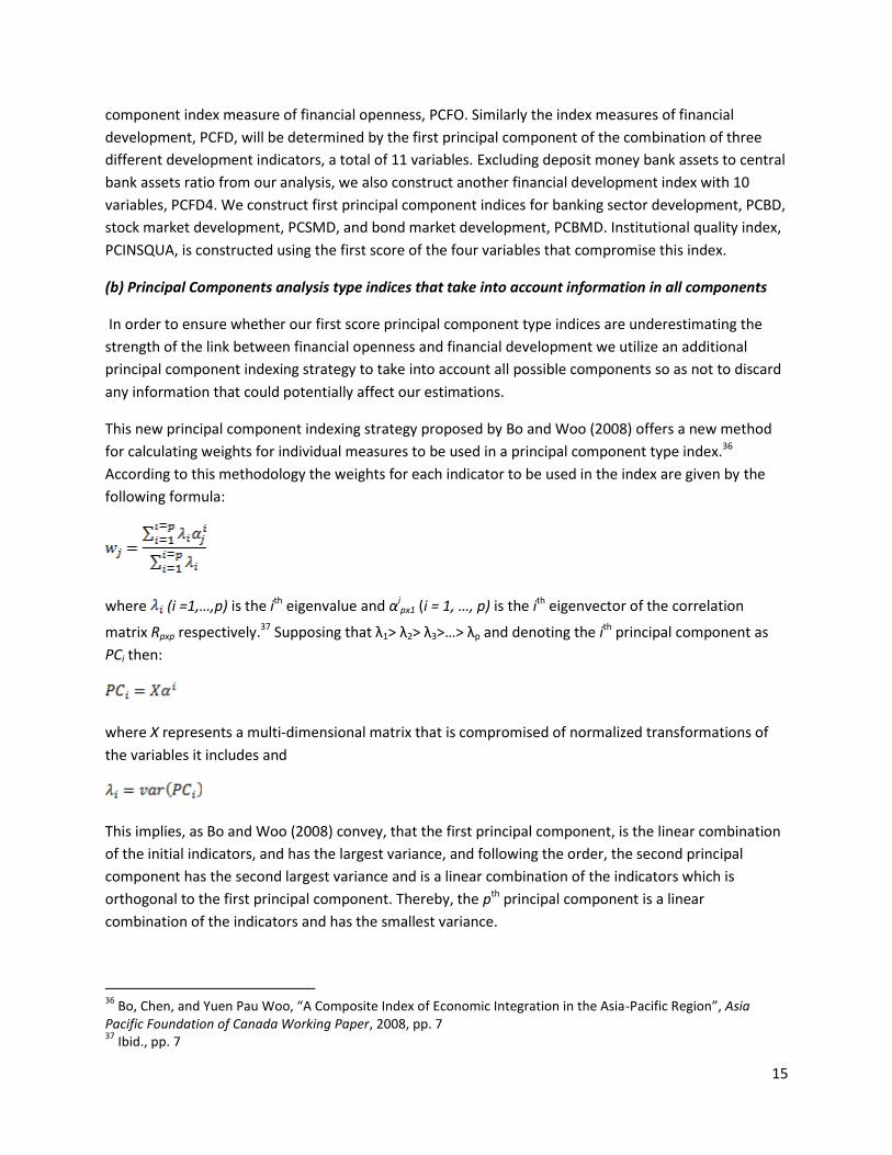
This new principal component indexing strategy proposed by Bo and Woo (2008) offers a new method
for calculating weights for individual measures to be used in a principal component type index.36
According to this methodology the weights for each indicator to be used in the index are given by the
following formula:
where (i =1,…,p) is the ith eigenvalue and αipx1 (i = 1, …, p) is the ith eigenvector of the correlation
matrix Rpxp respectively.37 Supposing that λ1> λ2> λ3>…> λp and denoting the ith principal component as
PCi then:
where X represents a multi-dimensional matrix that is compromised of normalized transformations of
the variables it includes and
This implies, as Bo and Woo (2008) convey, that the first principal component, is the linear combination
of the initial indicators, and has the largest variance, and following the order, the second principal
component has the second largest variance and is a linear combination of the indicators which is
orthogonal to the first principal component. Thereby, the pth principal component is a linear
combination of the indicators and has the smallest variance.
36
Bo, Chen, and Yuen Pau Woo, “A Composite Index of Economic Integration in the Asia-Pacific Region”, Asia Pacific Foundation of Canada Working Paper, 2008, pp. 7 37
Ibid., pp. 7
16
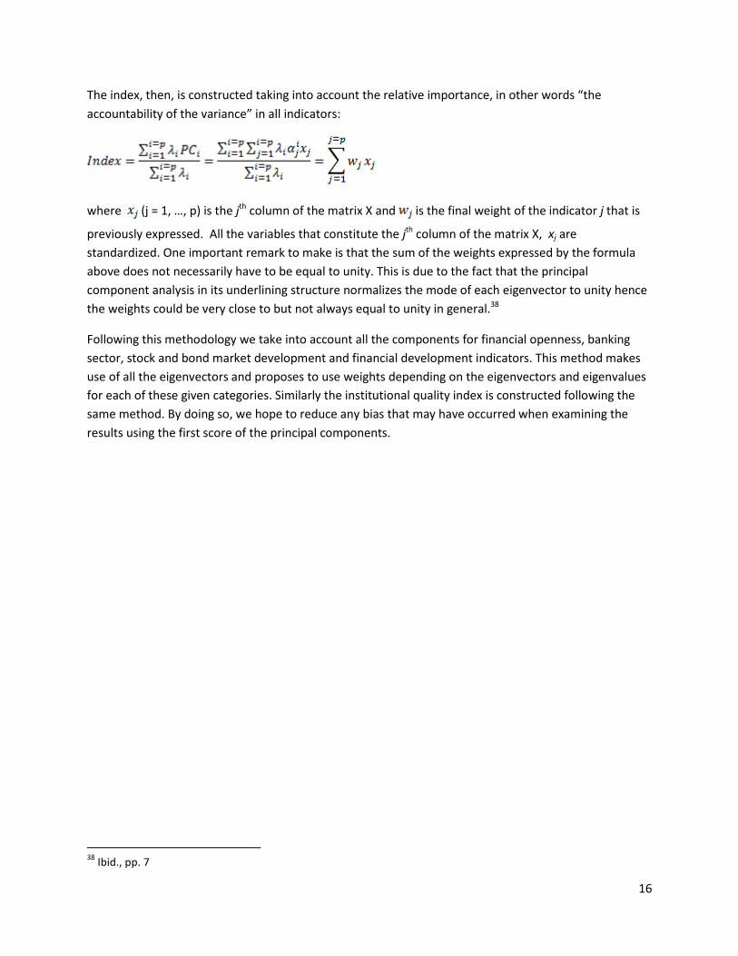
The index, then, is constructed taking into account the relative importance, in other words “the
accountability of the variance” in all indicators:
where (j = 1, …, p) is the jth column of the matrix X and is the final weight of the indicator j that is
previously expressed. All the variables that constitute the jth column of the matrix X, xj are
standardized. One important remark to make is that the sum of the weights expressed by the formula
above does not necessarily have to be equal to unity. This is due to the fact that the principal
component analysis in its underlining structure normalizes the mode of each eigenvector to unity hence
the weights could be very close to but not always equal to unity in general.38
Following this methodology we take into account all the components for financial openness, banking
sector, stock and bond market development and financial development indicators. This method makes
use of all the eigenvectors and proposes to use weights depending on the eigenvectors and eigenvalues
for each of these given categories. Similarly the institutional quality index is constructed following the
same method. By doing so, we hope to reduce any bias that may have occurred when examining the
results using the first score of the principal components.
38
Ibid., pp. 7
17
3. Empirical Model
Panel data models with cross sectional and time series data have been commonly used in financial
liberalization, economic growth and financial development literature. These models provide a powerful
approach in bringing together large number of countries across time to analyze and identify country-
specific effects that control for missing or unobserved variables.39 Unfortunately there are
disadvantages in using panel data models. Panel data models can cause complexities in the estimation
procedure. These types of models cannot be fully relied on determining the causal link between
financial liberalization and economic performance measures such as growth.40 There may also be large
finite sample biases when the instruments selected are weak.41 However, in our context, using panel
data models and in particular dynamic panel data estimation techniques will allow our financial
development and financial openness indicators to (partially) adjust to their long run equilibrium values
within a specified number of years.42 Via dynamic panel data models our estimates will no longer be
biased by any omitted variables such as country specific effects, and using instruments will assist in
overcoming problems of endogeneity and measurement error. With dynamic panel data models we will
not only be examining the cross-country variation in the data but also observing the effects of time-
series variation.
There have been various approaches employed in literature for the estimation of the link between
financial openness and financial development. While Chinn and Ito (2006) utilize simple, point estimate
OLS models, Huang (2006) argues for fixed effects estimation with levels, OLS estimation with first
differenced variables, and Arellano-Bond dynamic panel data model approach with GMM estimators.
Baltagi, Demetriades, and Law (2007) find dynamic panel data estimation models using the GMM case
suggested by Arellano-Bond more appropriate, whereas Demetriades and Law (2006) use two dynamic
panel data models, a first differenced panel GMM model, and the pooled mean group model.
In a standard static specification of the problem, we have that43:
39
Judson, Ruth A., and Ann L. Owen, “Estimating Dynamic Panel Data Models: A Practical Guide for Macroeconomists”, Federal Reserve Board of Governors, (1996), pp. 2 40
Aziakpono, Jesse Meshach, “Effects of Financial Integration on Financial Development and Economic Performance of the SACU countries”, Paper presented at the ECA/ADB African Economic Conferences, (2007), pp. 3 41
Bond, Stephen R., Anke Hoeffler, and Jonathan Temple, “GMM Estimation of Empirical Growth Models”, University of Oxford Economics Papers, 2001, pp. 5 42
Baltagi, Badi, Panicos Demetriades, and Siong Hook Law, “Financial Development, Openness, and Institutions: Evidence from Panel Data”, Paper presented at the IMF Conference on New Perspectives on Financial Globalization, 2007, pp. 11 43
Huang, Wei, “Emerging Markets, Financial Openness, and Financial Development”, University of Bristol Discussion Paper, 2006 – 588, pp. 15

18
where is the financial development measure, is the financial openness measure, is
the group of all control variables; trade openness, GDP growth, logarithm of GDP per capita, secondary
school enrollment rate, and institutional quality variables. The term is given to represent a country
specific effect that is captured neither by the financial openness indicators nor by the control variables.
This country fixed effect is used as a control for unobserved heterogeneity and is thought to differ
among countries. 44 is the coefficient on financial openness measures which we expect to be positive.
captures the total effect of financial openness on financial development and helps determine the
effectiveness of the link between the two. The error term is assumed to satisfy the Gauss-Markov
conditions.45 Dealing with unobserved heterogeneity that is present in the above model one can refer to
the within-group fixed effects estimator and first differences regression model. Unfortunately neither
model captures the partial adjustment property that accounts for the new information that explanatory
variables can bring to the dependent variable of financial development.46 Given that the dynamic panel
data models include this property, we prefer to use this type of a model in comparison to within-group
fixed effects estimators, or first differences regression models. Dynamic panel data model introduces a
method for modeling partial adjustment of variables. In order to obtain consistency in dynamic panel
data estimations we use the Arellano-Bond GMM panel data procedure to avoid the Nickell bias which
occurs when the lagged dependent variable is correlated with the disturbance. The country fixed effects
that are included in the dynamic panel data model suffer from this bias which disappears only if the time
variable T tends to infinity.47 Ultimately our Arellano-Bond (DIF – GMM) panel data model of 61
countries and twelve years, 1996 – 2007, can be given as:
where measures the speed of adjustment, and denotes the short run effect of the first difference
of financial openness on the first difference of financial development. Any influence of financial
openness is now conditioned on the history controlled by the first differenced lagged dependent
variable.48
The above model no longer has a country specific effect. The Arellano-Bond dynamic panel data model
accounts for the individual effects. We can observe that all terms have been differenced in order to
elude the Nickell bias. The inclusion of the lagged dependent variable helps remove any autocorrelation
that is present in the model. The moment conditions require that:
44
Ibid., pp. 15 45
Ibid., pp. 15 46
Ibid., pp. 19 47
Baltagi, Badi, Panicos Demetriades, and Siong Hook Law, “Financial Development, Openness, and Institutions: Evidence from Panel Data”, Paper presented at the IMF Conference on New Perspectives on Financial Globalization, 2007, pp. 11 48
Huang, Wei, “Emerging Markets, Financial Openness, and Financial Development”, University of Bristol Discussion Paper, 2006 – 588, pp. 17
19
This condition guarantees the lagged dependent variable to be uncorrelated with the first difference of
the error terms although the first difference of the lagged dependent variable could easily be correlated
with the first difference of the error terms. The moment conditions in the Arellano-Bond dynamic panel
data model increase with the time horizon, T.49 Two diagnostic tests for serial correlation are derived by
the model. These tests explore first order and second order serial correlation in error terms. The null
hypothesis in these tests supposes no serial correlation in disturbances. In our tests we expect to find
first order serial correlation in the first differenced residuals because and contain the same
term, that is .50 Second order and higher serial correlations could create further problems because
then we would not be able to verify the validity of the moment conditions.
To test for the over identifying restrictions in our model we perform Sargan tests. Since using a large
number of moment conditions may introduce bias while increasing efficiency we allow for one lag of the
dependent variable to be used as a right hand side regressor, and one lag of the variables other than the
dependent variable to be used as instruments for our moment conditions. We do not use the dependent
variable as an instrument in our estimations.
Given our model background, following Baltagi, Demetriades, and Law (2007), we test for the following
hypotheses:
I. (a) Do both trade and financial openness influence financial development and what happens to
financial development when we control for trade openness?
(b) Is simultaneous opening of both trade and capital accounts a necessary condition for financial
development? 51Do we examine a complementarity between the two? If the latter is true we will then
need to introduce an interaction term into the regression analysis to account for this simultaneity factor.
II. (a) What are the effects of economic and legal institutions on financial development over and above
the effects of openness?52
(b) Do educational indicators affect financial development?
Following these two hypotheses with two similar extensions, we can specify the following dynamic
equations for financial development:
49
Baltagi, Badi, Panicos Demetriades, and Siong Hook Law, “Financial Development, Openness, and Institutions: Evidence from Panel Data”, Paper presented at the IMF Conference on New Perspectives on Financial Globalization, 2007, pp. 11 50
Huang, Wei, “Emerging Markets, Financial Openness, and Financial Development”, University of Bristol Discussion Paper, 2006 – 588, pp. 18 51
Baltagi, Badi, Panicos Demetriades, and Siong Hook Law, “Financial Development, Openness, and Institutions: Evidence from Panel Data”, Paper presented at the IMF Conference on New Perspectives on Financial Globalization, 2007, pp. 5 52
Ibid., pp. 5
20
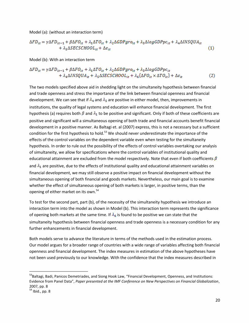
Model (a): (without an interaction term)
Model (b): With an interaction term
The two models specified above aid in shedding light on the simultaneity hypothesis between financial
and trade openness and stress the importance of the link between financial openness and financial
development. We can see that if and are positive in either model, then, improvements in
institutions, the quality of legal systems and education will enhance financial development. The first
hypothesis (a) requires both and to be positive and significant. Only if both of these coefficients are
positive and significant will a simultaneous opening of both trade and financial accounts benefit financial
development in a positive manner. As Baltagi et. al (2007) express, this is not a necessary but a sufficient
condition for the first hypothesis to hold.53 We should never underestimate the importance of the
effects of the control variables on the dependent variable even when testing for the simultaneity
hypothesis. In order to rule out the possibility of the effects of control variables overtaking our analysis
of simultaneity, we allow for specifications where the control variables of institutional quality and
educational attainment are excluded from the model respectively. Note that even if both coefficients
and are positive, due to the effects of institutional quality and educational attainment variables on
financial development, we may still observe a positive impact on financial development without the
simultaneous opening of both financial and goods markets. Nevertheless, our main goal is to examine
whether the effect of simultaneous opening of both markets is larger, in positive terms, than the
opening of either market on its own.54
To test for the second part, part (b), of the necessity of the simultaneity hypothesis we introduce an
interaction term into the model as shown in Model (b). This interaction term represents the significance
of opening both markets at the same time. If is found to be positive we can state that the
simultaneity hypothesis between financial openness and trade openness is a necessary condition for any
further enhancements in financial development.
Both models serve to advance the literature in terms of the methods used in the estimation process.
Our model argues for a broader range of countries with a wide range of variables affecting both financial
openness and financial development. The index measures in estimation of the above hypotheses have
not been used previously to our knowledge. With the confidence that the index measures described in
53
Baltagi, Badi, Panicos Demetriades, and Siong Hook Law, “Financial Development, Openness, and Institutions: Evidence from Panel Data”, Paper presented at the IMF Conference on New Perspectives on Financial Globalization, 2007, pp. 8 54
Ibid., pp. 8

21
the previous section avoid any problems that may result due to measurement errors55, we believe that our
results will provide a more advanced view of the effects of financial openness on financial development. We
hope to complement the work by Baltagi, Demetriades, and Law (2007) by a more thorough examination of
the simultaneity effect with our new unbiased index measures for financial openness and financial
development and by further studying the relationship between the two concepts. Given our initial objective
of establishing the importance of financial development as an element influencing economic growth and
welfare, and given that the literature has yet to find an answer to why we see differences among countries
in terms of extracting the advantages of financial liberalization, our analysis stands as a major starting point
for determining the transition mechanism between financial liberalization and financial development.
There remain to be a few drawbacks to our estimation model. The literature shows that in many cross-
sectional studies both developing and developed countries are lumped together in the same sample.56 As
Henry (2006) explains, including both sets of countries increases the sample size and could lead to more
efficient results in estimation, however, doing so without employing an empirical methodology which
particularly recognizes the fundamental theoretical difference between developed and developing
countries, would undermine the study’s ability to interpret the data.57 In order to correct the problem, we
first estimate our model with a full sample and then divide the sample into two components, developing and
developed countries so as to compare the results obtained in both estimation procedures. Another possible
drawback occurs due to the heavy influence of the control variables on financial development. As stated
previously the effect of financial development may be highly influenced by institutional quality and
educational attainment measures rather than the financial openness variable in which we are mostly
interested. In order to avoid this problem of mixing effects of the explanatory variables on the dependent
variable we exclude institutional quality and educational attainment indicators in some of our estimations.
We believe that by doing so we can obtain a better estimate for the actual effect of financial openness on
financial development.
55
Our index measures allow the data to tell us how to measure the concepts of financial openness and financial development. By avoiding any particular individual choices regarding measures for these two concepts and by examining the effects of different sectors on financial openness and financial development, we strongly argue that index measures will help avoid measurement problems that have been brought to the literature with particular use of individual measures. 56
Henry, Peter, “Capital Account Liberalization: Theory Evidence, and Speculation”, CDDRL Working Paper, (2006), pp. 16 57
Ibid., pp. 16

22
4. Empirical Results
We discuss the results of the dynamic panel data models introduced previously in this section. Table 1 in the
Appendix gives a brief summary of the variables used in our estimation procedure.
Examining the summary table reported in the Appendix, we can see that among all of our indices the equally
weighted banking sector development index, EBD, the equally weighted financial development index, EFD,
the coefficient of variation type banking sector development index, CBD, and the coefficient of variation
type financial development index, CFD, have the highest variabilities. This is caused by the high volatility of
deposit money bank assets to central bank assets ratio. This variability could be explained by the behavior of
individuals demanding deposit money bank assets under certain conditions and revising their decisions once
faced with uncertainty which can be triggered by recessionary periods. In order to avoid this bias from
causing mis-measurement problems in our indices we construct equally weighted, coefficient of variation
type and principal component type indices for financial development which discard the deposit money bank
assets to central bank assets ratio. 58
Tables 2 (a) to (d) show the relations of the index measures and the control variables. In Table 2 (a) we can
observe that the equally weighted financial openness index is positively correlated to all of our equally
weighted development indices. One surprising finding is to remark that the equally weighted financial
development index, EFD, is determined fully by the effect of the equally weighted banking sector
development index, EBD. Once deposit money bank assets to central bank assets ratio is excluded from our
index measures, the problem of one-to-one correlation between financial development and banking sector
development indices disappears, however, there still remain to be high correlations among the two indices
in comparison to the bond and stock market development indices. Even though the results of the pairwise
correlations reported in Table 2 (a) may have strong implications for our estimations we argue here that
these results may occur due to improper indexing techniques. An equally weighted index measure may not
be the best indicator to use but note that this problem could also be caused by the large variability of the
banking sector indicators as a whole. Consequently, some of the individual variables used to construct the
equally weighted banking sector development indicator may not be appropriate in this context.
Table 2 (b) shows the pairwise correlation results for coefficient of variation type indices. We again examine
a one-to-one correlation between coefficient of variation type banking sector development index, CBD, and
the financial development index, CFD. Another important remark to make concerns the negative
correlations of GDP growth with banking sector development index excluding deposit money bank assets to
central bank assets ratio, CBD1, bond market development index, CBMD, and financial development index
excluding the deposit money bank assets to central bank assets ratio, CFD4.
In Table 2 (c) we are given the pairwise correlations between first score principal component type indices
and control variables. The results show that all index measures have high correlations among each other,
58
The tables in the Supplementary Analysis show that the deposit money bank assets to central bank assets ratio have a 1-to-1 correlation with the equally weighted and coefficient of variation type banking sector development indices. Since this variable is found to have a great influence on our banking sector development indices, we presume that the exclusion of this variable will resolve any problems related to mis-measurement.
23
with financial openness index having a higher correlation for banking sector and overall financial
development indices. The banking sector development indices seem to have higher correlations with the
overall financial development indices which match the results found by Huang (2006). GDP growth again is
shown to have a high correlation with most of our indexing measures. The interaction term is found to be
positively correlated with both openness measures.
Lastly Table 2 (d) gives the pairwise correlations between principal component type indices that take into
account the information from all components and control variables. The financial openness index is again
found to be highly correlated with banking sector and overall financial development indices. There still
remain to be high correlations between financial development and banking sector development indices
however the results are more settled in comparison to those found in Table 2 (a).
4.1 Results using equally weighted index measures
Our empirical estimations for equally weighted indices are presented in Table 4 (a). In the benchmark
dynamic GMM estimations, all variables other than the lags of the dependent variable are treated as
exogenous. This method bares the assumption that all the right hand side regressors are uncorrelated with
the error term.59 We employ six different dependent variables in our regressions. The dependent variables
of the equally weighted indexing measure include the banking sector, bond and the stock market, and
financial development indices.
61 developing and advanced countries are covered in our analysis and the regressions are over a 12 year
period. The t-statistics reported in our regressions are based on standard errors. In addition to reporting the
results of dynamic panel data regressions, we also report the test for first and second order serial
correlation in disturbances, and the Sargan test for over-identifying restrictions.
The results in Table 4 (a) show that the equally weighted financial openness index, EFO, is statistically
significant for all dependent variables. Financial openness index enters with a positive coefficient for the
banking sector, bond and stock market and overall financial development indices when the most volatile
variable of banking sector is excluded from our analysis. This finding agrees with Huang (2006) where he
shows the equally weighted financial openness index to be mostly significant when regressed against the
first score principal component indices of banking sector, stock market and overall financial development.
Baltagi et. al (2007) report that for individual measures of banking sector development, their financial
openness index of total foreign assets and liabilities (%of GDP) is found to be positive and significant only
when private credit, domestic credit, and liquid liabilities are used as measures of banking sector
development. Law and Demetriades (2006) show that private capital flows which is used as a capital account
openness indicator along side to institutional quality variable and real GDP per capita all have a positive
significant impact on banking sector development indicator which is compromised of liquid liabilities, private
sector credit and domestic credit provided by the banking sector. The authors also find a positive and
significant relationship between the capital account openness measure of private capital inflows and stock
59
Baltagi, Badi, Panicos Demetriades, and Siong Hook Law, “Financial Development, Openness, and Institutions: Evidence from Panel Data”, Paper presented at the IMF Conference on New Perspectives on Financial Globalization, 2007, pp. 11

24
market development indicators of stock market capitalization, total share value traded and the number of
companies listed using pooled mean group estimates. Their results indicate that the coefficients of real GDP
per capita and institutional quality variable are positive and statistically significant throughout. Trade
openness is found to be significantly influencing the stock market development when stock market
capitalization and number of companies listed are used as the main indicators.
The rest of our results from Table 4 (a) indicate that the trade openness is positive and significant for
banking sector, EBD1, bond and stock market development, EBMD and ESMD, and financial development,
EFD4 indices, whereas GDP growth is significant for all dependent variables with changing magnitudes. GDP
growth has positive coefficients for stock market and overall financial development indices and negative
coefficients for banking sector and bond market development indices. This may imply that higher growth
leads to a decline in banking sector and bond market development. As Baltagi et. al (2007) express, the
negative coefficient of GDP growth may be related to counter-cyclicality of monetary policy.60 This could be
result of the sample being dominated by the advanced economies that face smaller GDP growth rates but
have well developed bond markets.
Both secondary school enrollment rate and equally weighted institutional quality index are found to be
negatively significant for almost all dependent variables. This finding contravenes the literature which states
that the effects of higher development in terms of institutions should be carried out to all sources of
financial development. Baltagi et. al (2007) using individual dependent variables find institutional quality
variable to be positive whenever it is significant, so our finding stands against the literature and remains to
be unresolved. We believe that our finding maybe the result of our indexing methodology, or due to the
choice of our institutional quality variables.
The results of the diagnostic tests show that in four out of six cases the first order serial autocorrelation is
rejected whereas the second order is accepted, and the Sargan test cannot reject the null hypothesis in all
cases thereby implying identification of our model.
Our results are in line with those found in the literature. We propose an addition of the bond market into
our financial development structure and the findings also highlight the importance of the link between
financial openness and bond market development.
4.2 Results using coefficient of variation type index measures
Table 4 (b) depicts the results of coefficient of variation type index measures. Financial openness index is
found to be significant for all dependent variables however the coefficients are positive only when banking
sector development that excludes the deposit money bank assets to central bank assets ratio, stock market
development, and both financial development indices are used as dependent variables. Similarly trade
openness is found to be positively significant for stock and bond market, and banking sector and financial
development indices that exclude the most volatile variable of the banking sector. GDP growth is shown to
have a negative coefficient for almost all cases with an exception of stock market and overall financial
development index, CFD4. Secondary school enrollment rate is again found to be negatively significant for
60
Ibid., pp. 12
25
all cases with the exception of bond market development whereas the coefficient of variation type
institutional quality index is negative and significant for all cases. The first order serial correlation is rejected
in four out of six cases and the Sargan test cannot reject the null hypothesis of over-identification for all
cases.
The coefficient of variation type indices depict similar results to the ones found using equally weighted
indices. Given that the structure of these indices depend greatly on standard deviations of individual
variables used in compiling index measures we would expect to find clearer relationships between openness
and development measures. However, the results show that the financial openness and development link is
better captured when using equally weighted indices.
4.3 Results using principal component analysis type index measures
In order to formally apply the principal component analysis to construct indices for financial openness,
financial development and institutional quality we first need to verify whether the individual variables that
are to be used in our indices are correlated. Our results show that we have positive correlations among most
of our individual variables. Following these results, we proceed on to using the principal component analysis
in constructing index measures.
4.3.1 Results using first principal components
We construct principal component indices using the first components (scores). Following this methodology
we score the first principal component of financial openness, PCFO, which consists of five individual
measures as described previously in Section 3. Similarly the index measure of financial development, PCFD,
will be determined by the first principal component of the combination of three different development
indicators, a total of 11 variables. We also score index measures using the first components for banking
sector development, PCBD, stock market development, PCSMD, and bond market development, PCBMD. In
order to examine whether the results are highly influenced by the most volatile variable of the banking
sector development index, deposit money bank assets to central bank assets ratio, we score index measures
for banking sector development, PCBD1 and financial development, PCFD4, that exclude this particular
variable.
The results for the first principal component of financial openness, in Table 3 (a), show that this component
captures 26.56% - 58.06 % of the total variation of individual measures depicted in terms of eigenvectors.
The total variation here refers to the maximal amount of variation in all five observed variables. PCFO, the
first component of financial openness index, is shown to capture 49.67% of the entire variance of 5
individual indicators of financial openness. Since most of these variables are observed to have similar
eigenvectors which represent their respective weights in the principal component analysis structure,
constructing an index measure of financial openness using the first principal component measure yields
accurate and sensible results.61 Given similar weights that are expressed by eigenvectors which range from
0.2656 – 0.5806, using any single measure to study the impact of financial openness on financial
61
Huang, Wei, “Emerging Markets, Financial Openness, and Financial Development”, University of Bristol Discussion Paper, 2006 – 588, pp. 12

26
development would bias our results. We thereby use the first principal component to score a proper and an
efficient index for financial openness.
Similarly the results of the principal component analysis for banking sector development in Table 3 (b) show
that the first principal component of banking sector development captures 27.89 % - 48.92 % of the total
variation of individual measures. One must note that the deposit money bank assets to central bank assets
ratio is found to have a negative sign in the first principal component of the PCBD, the first principal
component of banking sector development index. PCBD, overall, captures 60.72% of the entire variance of 6
individual indicators of banking sector development. Excluding deposit money bank assets to central bank
assets ratio from the individual variables that compromise the banking sector development index increases
the overall significance of the first component of banking sector development index, as shown in Table 3 (c).
Without deposit money bank assets to central bank assets ratio the first principal component of banking
sector development, PCBD1, captures 28.03% - 48.94 % of the total variation of individual measures. PCBD1,
summarizes 72.77% of the entire variance of 5 individual indicators of banking sector development
compared to the 60.72% that PCBD index captures.
The results of principal components analysis on bond market development depicted in Table 3 (d) show that
the first component explains 67.26% of the total variation of the two individual indicators. Since the number
of individual variables forming this index is relatively small we are assured that the first component will be
enough in capturing the total effects of the principal component analysis.
The first principal component of stock market development in Table 3 (e), on the other hand, is found to
capture 48.64% - 68.59 % of the total variation of individual measures. PCSMD, the first component of stock
market development index, overall, captures 65.57% of the entire variance of 3 individual indicators of the
stock market development.
Lastly the results of the principal component analysis for financial development, in Table 3 (f), show that the
first principal component of the financial development index explains 46.28% of the total variation of 11
variables that construct banking sector, stock market and bond market development indices. The
eigenvectors of the first principal component of financial development are all positive and similar, capturing
12.22 % - 41.01% of the total variation of individual measures. Among all 11 measures only deposit money
bank assets to central bank assets ratio has a negative eigenvector. When we exclude this variable from our
principal component index of financial development, in Table 3 (g), the proportion explained by the first
component rises up to 50.82% and all the eigenvectors in the first component are found to be positive.
For the institutional quality index we score the first principal component of government effectiveness,
regulatory quality, rule of law, and control of corruption. The total proportion, the variance, explained by
the first component, is 95.90% as shown in Table 3 (h). The eigenvectors are also found to be very similar
ranging between 49.35% - 50.41%.
The results strongly verify our choice of principal component type indices for financial openness, banking
sector, bond and stock market, financial development and institutional quality indices. We observe
eigenvectors which suggest that using individual variables in our analysis to examine the link between
27
financial openness and financial development would not gather all the information that can possibly be
captured through the use of principal component indices.
Table 4 (c) shows our first results of principal component indices. The results show that the financial
openness index, PCFO, is found to be significant in all cases with the exception of bond market development
index. In all five cases the financial openness index has a positive and statistically significant coefficient
which argues that financial openness contributes to the development of banking sector, stock market and
overall development of financial markets. Likewise trade openness is found to be positive and significant for
all dependent variables. This could imply that trade openness affects the development of bond markets
whereas financial openness does not have a significant effect on the overall enhancement of bond markets.
The estimated coefficients for trade and financial openness for all dependent variables suggest that the
openness indices are economically meaningful.
The control variables of institutional quality index and secondary school enrollment rate are mostly found to
be significant however with differing magnitudes. Secondary school enrollment rate enters with a positive
coefficient in three out of six cases, whereas institutional quality is once again found to be negatively
significant in four out of six cases. The diagnostics are satisfactory for all dependent variables used. The
absence of first order serial correlation is rejected and the Sargan test results cannot reject the over-
identification restrictions.
Overall, our findings show that there is a significant link between financial openness and financial
development when we index both measures using principal component analysis. The results also
demonstrate that working with first score principal component indices, the link between financial openness
and financial development becomes more comprehensible. We obtain better and economically more
meaningful results using the first score principal component analysis in comparison to using equally
weighted and coefficient of variation type indices. GDP growth and secondary school enrollment rate enter
with positive and highly significant coefficients under first score principal component indices than under
equally weighted or coefficient of variation type indices. However, one intricate observation is that with first
score principal component indices we can no longer find a link between financial openness and bond market
development.
Huang (2006) reports similar results to our initial estimations. He finds financial openness index constructed
using the first principal components to be positive and significant for stock market, banking sector and
financial development. Nevertheless, our estimations using the first score of the principal component
analysis match well with the results obtained in the literature.
4.3.2 Results using a new methodology of principal components
Using the corresponding weights determined by the principal component analysis taking into account all
components and their corresponding eigenvalues, we construct our indices taking the standardized
individual measures and multiplying them with these corresponding weights. This method allows us to have
all variables in a range of values and avoids any potential problem that could arise as a result of using
different scales or units of measurement.
28
The results in Table 4 (d) indicate that the financial openness index is significant for all dependent variables.
Trade openness is also found to be significant and positive for all cases. GDP growth is significant for all
cases with an exception of the second banking sector index, PCABD1,whereas logarithm of GDP per capita is
significant and positive for banking sector and stock market indices. First order serial autocorrelation tests
are rejected for all cases, while the Sargan test of over-identification cannot reject the null hypothesis in all
cases.
Our results show that using further components in our indexing strategy appears to offer similar findings in
examination of the link between financial openness and financial development to using the first principal
component indexing strategy. Due to the similarity of the results employing both types of principal
component indices, it is difficult to identify one methodology as the ideal procedure in constructing index
measures. Further examination of Tables 4 (c) and (d) shows that while first score indices give higher
significances in terms of t-statistics, the new methodology provides better results in terms of magnitudes
and stands to be more economically meaningful in terms of interpretations. As a result, we restrain from
using other type of indices such as equally weighted and coefficient of variation for further results, and we
report the following results using our most efficient methodology of principal components.
4.4 Adding the interaction term
In order to examine the effect of a simultaneous opening of both trade and financial markets on financial
development, we estimate our Model (b) given in equation (2). The results for new methodology of principal
components are reported in Table 5.
The results from Table 5 demonstrate that the financial and trade openness index are positive and
significant under all regressions. GDP growth is positive and significant for banking sector, stock market and
financial development indices and logarithm of GDP per capita is positive and significant only for banking
sector development indices. Institutional quality index is negatively significant for bond and stock market
development indices and positively significant for financial development index, PCAFD4 whereas secondary
school enrollment rate is positively significant for banking sector development index, and negatively
significant for stock market and financial development indices. The interaction term between financial and
trade openness is shown to be significant but negative in all cases. This finding is intriguing as it implies that
a simultaneous opening of both markets leads to a decline in banking sector, stock, bond and overall
financial development. This may be due to the effects of financial openness and trade openness being
picked up separately by each variable and not particularly by the interaction term. Our results mostly agree
with those found in the literature. Baltagi et. al (2007) find the interaction term to be statistically significant
together with financial and trade openness when the stock market development indicator is taken to be the
number of companies listed. Using banking sector development measures as the dependent variable, the
authors find the interaction term to be significant and negative for private credit, liquid liabilities and
domestic credit. Interestingly their results show that the coefficients of the financial openness terms are
positive and large whereas the interaction term has negative coefficients. Law and Demetriades (2006) find
the interaction term, trade openness and capital account openness measured by private capital flows to be
statistically significant and positive when stock market capitalization, total share value traded and the
number of companies listed are used as individual indicators of stock market development.

29
Our findings suggest that the use of index measures is beneficial in examining the link between financial
openness and financial development. In order to check sensitivity of our results to potential outliers we
proceed to robustness checks.

30
5. Robustness checks and further issues
We carry out a large number of robustness checks in order to examine sensitivity of our results to
alternative specifications and methods. Here, we only report a subset of these robustness checks. A further
issue that complicates our findings is also considered in this section. Below we discuss the results when the
issue of endogeneity in our sample is taken under examination. Breaking the data set into developing and
advanced countries we investigate whether our results hold when only developing countries are taken into
consideration.
5.1 Robustness checks
The first set of robustness checks involves adjusting variables by their respective means. Dividing each
individual variable in index measures by their means we can construct new indices for financial openness,
financial development and institutional quality. Adjusting variables by their means, we can obtain principal
component indices employing the new methodology suggested in section 3. However, due to the structure
used by principal component analysis the mean adjusted indices depict the same components as the non-
mean adjusted original ones. Adjusting the variables by their respective means before using the principal
components strategy does not alter the eigenvectors and eigenvalues used in construction of principal
components. The results (not reported here)62 match well with our previous findings, however, financial
openness index enters with a significantly negative coefficient for banking sector and bond market
development indices. For these three dependent variables we also find GDP growth and secondary school
enrollment rate to have negative coefficients. For stock market and financial development indices we
observe similar results to those given in Table 4 (d). The diagnostics for the Arellano-Bond serial
autocorrelation tests depict disappointing results for the first two dependent variables which help us confide
in our initial estimations using principal components and standardized variables in comparison to mean
adjusted ones.63
The second test of robustness checks concentrates on the number of observations used in our analysis. Due
to the data availability, some indices include a larger number of variables in comparison to others. Using
financial development indices as dependent variables, we would like to examine the results when the
number of observations for each dependent variable used in our estimations is equalized. By doing so, we
aim to minimize the bias that may result among different dependent variables as a result of problems of
missing observations. Table 6 depicts the results for this case. The results are similar to those found in Table
4 (d). When the number of observations for each regression is equalized only minor changes take place
according to the use of different dependent variables. Some control variables such as secondary school
enrollment rate and institutional quality index alter signs in Table 6.
62
Please refer to the Supplementary Appendix for the results of the mean adjusted indices. 63
Checking the robustness of equally weighted, coefficient of variation type and first score principal component type indices we find that the results are similar to the ones reported in Table 4. Similarly exclusion of institutional quality and secondary school enrollment rates from the regressions using these three index measures gives robust results. The exclusion of secondary school enrollment rate leads the trade openness term to take on a negative coefficient so we believe that this variable is of vital importance to our regressions. We can thereby confirm that our other index measures are robust to different estimation techniques.

31
Following up on robustness checks, we also seek to examine whether the exclusion of control variables of
secondary school enrollment rate and institutional quality index make a difference to our proposed model.
The exclusion of institutional quality index from our regressions whilst using the principal components type
indices of financial openness and financial development does not affect our initial findings. Similarly the
estimations with the exception of the secondary school enrollment rate show that trade openness loses
significance for some dependent variables and GDP growth and institutional quality index become more
significant with a negative coefficient for other dependent variables. These results show that even though
the exclusion of institutional quality does not remarkably change our results, the exclusion of secondary
school enrollment rate is enough to make our findings less economically meaningful. We thereby, stress the
importance of including both of these control variables in our analysis to examine the link between financial
openness and financial development.64
Further tests regarding the structure of the variables have also been taken into account. For brevity of the
discussion these results are not reported here. Treating all variables as predetermined does not alter our
main findings. With predetermined variables we find that trade openness enters with a negative coefficient
when banking sector and bond market development indices are used as dependent variables. Similarly
treating financial and trade openness as predetermined variables does not change our results. Lastly we
examine the effects of treating openness variables as endogenous. The results show large similarities to the
ones reported on Table 4 (d). We thereby confirm that the assumption of treating the right hand side
regressors as exogenous variables is not a restrictive one in our case.65
Another important issue considered is the time series versus cross sectional effects that influence our
model. Due to the twelve year period selected in our model we believe that there may be time series effects
that are not picked up by our one lag structure. In order to account for these effects we try a higher lag
model to observe whether our results are sensitive to different lag structures. Table 7 depicts the results
when three lags of the dependent variable are used as right hand side regressors and three lags of the
variables other than the dependent variable are used as instruments. The results show that adding lags does
not change our main findings. With further lags being used both as right hand side regressors and as
instruments we find that trade openness becomes insignificant for banking sector development index,
PCABD, and negatively significant for bond market development index. The dependent variables of
development indices show high time series persistence. GDP growth, logarithm of GDP per capita,
institutional quality and secondary school enrollment rate alter signs for some dependent variables.
Nevertheless, our results show improvement in diagnostics with Arellano-Bond serial autocorrelation tests.
Using other lag specifications and allowing for dependent variables to be used as instruments does not
change our main findings. We have restrained from using dependent variables as instruments in our main
analysis due to their unsuccessful diagnostics in terms of Sargan tests in comparison to the methods shown
in this paper. We have experimented that using other variables as instruments gives higher significances and
better diagnostic results than using dependent variables as instruments. However, our robustness checks
64
The table of results for the exclusion of institutional quality index and secondary school enrollment rate are not reported in this paper due to space limitations. The results are available in the Supplementary Appendix. 65
The results for all variables being treated as predetermined and endogenous can be found in the Supplementary Appendix.

32
with further lags do not modify our results. Our analysis with higher lags demonstrates that the qualitative
nature of our results is robust to alternative specifications and estimation methods.
We lastly explore how our benchmark results change when we consider not only time series effects but also
cross sectional effects in our model. In order to observe the changes we add time series dummies and a
country-specific time trend to account for differences across countries. The results are given in Table 8. We
do not report the entire set of results for all time dummies from 1996 to 2007. Due to collinearity dummies
for 1996 and 1997 are dropped. The results show that trade openness is only significant for stock and bond
market development when time dummies and a trend are included in the model to account for cross
sectional and time series dimensions. Logarithm of GDP per capita enters with negative signs in all cases.
The trend has a positive and significant coefficient for all dependent variables and the time dummy for the
year 1998 is positive and significant for four cases out of six. This implies that both cross-sectional and time
series effects have high influences on our model. By adding a trend we account for the differences across
countries in our sample. Examination of the time dummies not reported here66 shows that these dummies
are negatively significant for banking sector development indices whereas for stock and bond market, and
overall financial development indices some time dummies are found to be negatively and some positively
significant. The diagnostics are better when time dummies and a trend are included in our estimation
process. On the other hand adding more lags with time dummies gives similar results but further improves
the Arellano-Bond serial correlation and Sargan test results. By this means we confirm that our benchmark
results are robust to alternative estimation methods. Adding lags and time dummies to incorporate time
series effects and a trend variable to account for cross-sectional variation does not change the qualitative
nature of our results.
On a final note we examine the results when the most frequently used individual measures of financial
openness and financial development are regressed against index measures. Although it is not reported
here67 the findings convey mixed results for the relationship between financial openness and financial
development. Using individual measures as dependent variables for financial development, or using
individual variables as measures of financial openness we cannot find the clear link that we observe
between financial openness and financial development whilst using index measures. The results clearly
demonstrate that depending on the variables chosen, the relationship between financial openness and
financial development alters. This finding, once again, strengthens our argument that using index measures
we can evidently find a positive link between financial openness and financial development.
5.2 Further issues
As a last robustness check we examine the endogeneity problem that is existent in our model. As previously
explained, the use of developing and advanced countries together in our benchmark analysis can create a
drawback to our estimated model. Even though large number of observations in a joint sample brings more
efficient results we may not be able to fully differentiate whether the effects of financial openness on
financial development follow due to the influence of advanced economies in our joint data set. In order to
66
Please refer to the Supplementary Appendix for the full table with time series dummies and a linear trend, time series dummies and higher lags with time series dummies and a linear trend. 67
The results using individual measures can be found in the Supplementary Appendix.
33
avoid complications and to clarify the issue regarding the endogeneity problem we split our data set into
developing and advanced countries68 and examine the results when the developing country sample is used
in estimations.
The developing country sample includes 31 countries over the same twelve year period. Our results using
the same estimation methodology are reported in Table 9. The results show that financial openness is
positive and significant for all dependent variables used. The results are similar to those in Table 4 (d) in
terms of sign and significance for most variables; however, some variables such as trade openness, GDP
growth and secondary school enrollment are different in magnitudes. The diagnostics given in Table 9 satisfy
both Arellano –Bond serial correlation tests and the Sargan test of over-identification. The results, overall,
confirm that we do not have an endogeneity problem that is not explicitly recognized by our estimation
methods. The link between financial openness and financial development follows even when a subsample of
developing countries is used in our analysis. This strengthens the argument of the importance of opening up
financial markets in order to develop banking sector, bond and stock markets in developing countries. We
hereby reveal that financial openness does influence financial development in both developing and
advanced countries and the link between these two is more likely to affect growth and welfare of these
countries. The relationship examined here is important and should not be disregarded in an analysis of
welfare and growth differences across countries. Having shown that the discrepancies among countries in
terms of financial development might arise as a result of not fully opening up financially we leave the
analysis of financial openness, economic growth and welfare to another study.
68
We rely on the World Bank’s income group definition when splitting our data set into developing and advanced countries.

34
6. Concluding remarks
Even though the link between financial liberalization and economic growth has been widely examined, the
relationship between financial liberalization and financial development has yet to be thoroughly discussed.
Our main goal in this paper was to construct comprehensive indicators for financial openness and financial
development. By addressing the measurement problem through the use of index measures we were able to
thoroughly study this link.
Given the goal of using broad indicators for both financial openness and financial development through the
aid of aggregate indices in a large panel data set containing both developing and advanced countries we
studied the relationship between financial openness and financial development to the best of our
knowledge. Our results using aggregate indices with equal weights, coefficient of variation and two different
principal component type methodologies show that the relationship between financial openness and
financial development exists and it is more significant than what the literature has previously shown.
Further examination of our benchmark Arellano-Bond GMM results depict that the principal component
indices using all components provide higher significances and economically more meaningful
interpretations. In all estimations, independent of the development indices chosen, financial openness is
always found to be a positive and significant factor influencing financial development. The addition of an
interaction term, which is proposed to be an influential factor in determining whether the simultaneous
opening of financial and goods markets have further effects on financial development, brings intriguing
results. Our findings show that the interaction term is negatively significant implying that a simultaneous
opening of financial and goods markets may not be fully beneficial on financial development.
Additional robustness checks demonstrate that financial openness has a positive effect on financial
development independent from the lag structure chosen, and time dummies and trends used. The positive
influence of financial openness carries out even when the sample size is reduced to developing countries. By
breaking the sample into developing and advanced countries and by examining the results from the
developing country sample we can confirm that the link between financial openness and financial
development exists and this link is likely to be an influential factor in bringing about enhancements to
economic growth and welfare across countries. Even though our findings mostly report negatively significant
results for institutional quality, secondary school enrollment rate and GDP growth, we believe that these
variables are the most probable causes for the discrepancies across countries in terms of development
following financial liberalization.
On a last note, we have shown that using index measures with a large country sample and a broad selection
of control variables, the link between financial openness and financial development is unambiguous. To this
end, future work would call for a model that can provide theoretical underpinnings for the effects of
financial openness on financial development. By this means, we will be able to clearly examine the link
between financial openness and financial development, as well as economic growth and welfare through a
sound model that has the foundations to match macroeconomic theory with the results of estimations that
stem from the use of comprehensive financial indicators as reported here.

35
REFERENCES
Agenor, Pierre-Richard, “Does Globalization Hurt the Poor?”, The World Bank Working Paper, 2003
Alfaro, Laura, Sebnem Kalemli-Ozcan, and Vadym Volosovych, “Capital Flows in a Globalized World: The Role
of Policies and Institutions”, NBER Working Paper, 2005 – 11696
Arestis, Philip, Panicos O. Demetriades, Bassam Fattouh, and Kostas Mouratidis, “The Impact of Financial
Liberalization Policies on Financial Development: Evidence from Developing Economies”, University
of Leicester Department of Economics Discussion Paper 2002 – 01
Arestis, Philip, and Panicos O. Demetriades, “Finance and Growth: Institutional Considerations, Financial
Policies and Causality”, Keele University Department of Economics Discussion Paper, 1997 – 02
Arestis, Philip, and Panicos O. Demetriades, “Financial Development and Economic Growth: Assessing the
Evidence”, Economic Journal, 1997, Vol. 107, No. 442, pp. 783 – 799
Aziakpono, Jesse Meshach, “Effects of Financial Integration on Financial Development and Economic
Performance of the SACU Countries”, Paper presented at the ECA/ADB African Economic
Conferences, (2007)
Baltagi, Badi, Panicos Demitriades, and Siong Hook Law, “Financial Development, Openness, and
Institutions: Evidence from Panel Data”, Paper presented at the IMF Conference on New Perspectives
on Financial Globalization, 2007
Beck, Thorsten, and Asli Demirguc-Kunt, “Financial Institutions and Markets across Countries and Over Time
– Data and Analysis”, World Bank Working Paper, (2009), pp. 1 – 43
Beck, Thornsten, Asli Demirgüç-Kunt, and Ross Levine, "A New Database on Financial Development and
Structure," World Bank Economic Review 14, (2000), 597-605.
Bekaert, Geert, Campbell R. Harvey, and Christian Lundblad, “Emerging Equity Markets and Economic
Development”, Journal of Development Economics, (2001), Vol. 66, No. 2, pp. 465 – 504
Bekaert, Geert, and Campbell Harvey, “Economic Growth and Financial Liberalization”, NBER Reporter,
(Spring 2001), pp. 8 – 11
Bhagwati, Jagdish, "Why Free Capital Mobility May be Hazardous to Your Health: Lessons from the Latest
Financial Crisis”, NBER Conference on Capital Controls, (1998)
Bhagwati, Jagdish, In Defense of Globalization, Oxford University Press, 2005
Bo, Chen, and Yuen Pau Woo, “A Composite Index of Economic Integration in the Asia-Pacific Region”, Asia
Pacific Foundation of Canada Working Paper, 2008, pp. 1 – 27
36
Bond, Stephen R., Anke Hoeffler, and Jonathan Temple, “GMM Estimation of Empirical Growth Models”,
University of Oxford Economics Papers, 2001, pp. 1- 33
Burgoon, Brian, “Globalization and Welfare Compensation: Disentangling the Ties That Bind”, International
Organization, (Summer 2001), Vol. 55, No. 3, pp. 509-551
Chinn, Menzie, and Hiro Ito, “What Matters for Financial Development? Capital Controls, Institutions and
Interactions”, Journal of Development Economics, (2006), Vol. 81, No. 1, pp. 163 – 192
Chinn, Menzie, and Hiro Ito, “Capital Account Liberalization, Institutions and Financial Development: Cross
Country Evidence”, NBER Working Paper, 2002 – 8967
De la Torre, Augusto, and Sergio L. Schmukler, “Emerging Markets and Globalization: The Latin American
Experience”, Stanford University Press and World Bank, 2007
De Gregorio, Jose, “Financial Integration, Financial Development, and Economic Growth”, mimeo
Department of Industrial Engineering, Universidad de Chile, July 2000
Demetriades, Panicos O., and Siong Hook Law, “Openness, Institutions and Financial Development, WEF
Working Papers, 2006 – 0012
Demetriades, Panicos O., and Svetlana Andrianova, “Sources and Effectiveness of Financial Development:
What We Know and What We Need to Know”, World Institute for Development Economic Research
Working Papers, RP2005/76
Demetriades, Panicos O., and Siong Hook Law, “Finance, Institutions, and Economic Growth”, University of
Leicester Department of Economics Discussion Paper, 2005 – 04
Demetriades, Panicos O., and Siong Hook Law, “Capital inflows, trade openness and financial development
in developing countries”, Money Macro and Finance (MMF) Research Group Conference, 2004 – 38
Demetriades, Panicos O., and Khaled A. Hussein, “Does Financial Development Cause Economic Growth?
Time-Series Evidence from 16 Countries”, Keele University Department of Economics Discussion
Paper, 1995 – 13
Demirguc – Kunt, A., and A. Levine, “Stock Market Development and Financial Intermediaries: Stylized
Facts”, World Bank Economic Review, (1996), Vol. 10, pp. 291 – 322
Demirguc – Kunt, Asli, Thorsten Beck, and Ross Levine, “A New Database on Financial Development and
Structure”, The World Bank Policy Research Working Paper, 1999 – 2146
Demirguc-Kunt, Asli, and Ross Levine, Financial Structure and Economic Growth: A Cross-Country
Comparison of Banks, Markets, and Development, MIT Press, 2001
Dunteman, George H., Principal Components Analysis, Sage Publications, 1989

37
Easterly, William R., “Globalization, Inequality, and Development: The Big Picture”, Monetary and Economic
Studies, (Dec. 2004)
Eatwell, J., “International Financial Liberalization: The Impact on World Development”, United Nations
Development Program Discussion Paper Series, 1997 – 12
Edison, Hali, Ross Levine, Luca Ricci, and Torsten Slok, “International Financial Integration and Economic
Growth”, Journal of International Monetary and Finance, (2002), Vol. 21, pp. 749 – 776
Eichengreen, Barry J., “Capital Account Liberalization: What Do Cross-Country Studies Tell Us?”, World Bank
Economic Review, 2001, Vol. 15, pp. 341 – 365
Eichengreen , Barry, and M. Mussa, “Capital account liberalization: Theoretical and practical aspects”,
Journal of International Money and Finance, (2002), Vol. 21, pp. 749 – 776
Gourinchas, Pierre-Olivier, and Olivier Jeanne, “The Elusive Gains from International Financial Integration”,
NBER Working Paper, 2003 – 9684
Gourinchas, Pierre-Olivier, Olivier Jeanne, “Capital Flows to Developing Countries: The Allocation Puzzle”,
NBER Working Paper, 2007 – 13602
Henry, Peter, “Stock Market Liberalization, Economic Reform, and Emerging Market Equity Prices”, Journal
of Finance, (April 2000), Vol. 55, pp. 529 – 564
Henry, Peter, “Capital Account Liberalization: Theory, Evidence, and Speculation”, NBER Working Paper,
2006 – 12698
Henry, Peter, “Capital Account Liberalization, the Cost of Capital, and Economic Growth”, American
Economic Review, (2003), Vol. 93, pp. 91 – 96
Hoxha, Indrit, Sebnem Kalemli-Ozcan, and Dietrich Vollrath, “How big are the gains from international
financial integration”, NBER Working Paper, 2009 – 14636
Huang, Wei, “Emerging Markets, Financial Openness, and Financial Development”, University of Bristol
Discussion Paper, 2006 – 588
Ito, Hiro, “Financial development and financial liberalization in Asia: Thresholds, institutions and the
sequence of liberalization”, The North American Journal of Economics and Finance, (2006), pp. 303 -
327
Judson, Ruth A., and Ann L. Owen, “Estimating Dynamic Panel Data Models: A Practical Guide for
Macroeconomists”, Federal Reserve Board of Governors, (1996), pp. 1 - 21
Kaminsky, Graciela, and Sergio Schmukler, “Short-Run Pain, Long-Run Gain: The Effects of Financial
Liberalization”, NBER Working Paper, 2003 – 9787
38
Kaufmann, Daniel, Aart Kraay and Massimo Mastruzzi, “Governance Matters VIII: Governance Indicators for
1996-2008”, World Bank Policy Research, Paper number 4978, (2009), pp. 1 – 103
Kaufmann, Daniel, Aart Kraay and Massimo Mastruzzi, “The Worldwide Governance Indicators:
Methodology and Analytical Issues”, World Bank Policy Research, Paper number 5430, (2010
Klein, Michael, and Giovanni Olivei, “Capital Account Liberalization, Financial Depth, and Economic Growth”,
Tufts University, 2000
Kose, M. Ayhan, Eswar S. Prasad, Kenneth S. Rogoff, and Shang-Jin Wei, “Financial Globalization, Growth and
Volatility in Developing Countries”, NBER Working Paper, 2004 – 10942
Kose, M. Ayhan, Eswar S. Prasad, Kenneth S. Rogoff, and Shang-Jin Wei, “Financial Globalization: A
Reappraisal”, NBER Working Paper, 2006 – 12484
Kose, M. Ayhan, Eswar S. Prasad, Kenneth S. Rogoff, and Shang-Jin Wei, “The Effects of Financial
Globalization on Developing Countries: Some Empirical Evidence”, IMF Occasional Paper, (2003), No.
220
Lane, Philip R., and Gian Maria Milesi-Ferretti, “International Financial Integration”, IMF Working Paper,
2003 – WP 03/86
Law, Siong Hook, and W.N.W Azman Saini, “The Quality of Institutions and Financial Development”, MPRA
Paper 12107, (2008), pp. 1 -18
Levine, Ross, “International Financial Integration and Economic Growth”, Review of International Economics,
(2001), Vol. 9, No. 4, pp. 684 – 698
Levine, Ross, Norman Loayza, and Thorsten Beck, “Financial intermediation and growth: Causality and
causes”, Journal of Monetary Economics, (2000), Vol. 46, pp. 31 – 77
Levine, Ross, and Sara Zervos, “Capital Control Liberalization and Stock Market Development”, World
Development, (1998), Vol. 26, No. 7, pp. 1169 – 1183
Lucas, Robert E. Jr., “Why Doesn’t Capital Flow from Rich to Poor Countries?”, American Economic Review,
(1990), Vol. 80, pp. 92 – 96
Martin, Philippe, and Helene Rey, “Globalization and Emerging Markets: With or Without Crash?”, The
American Economic Review, (Dec. 2006), Vol. 96, No. 5, pp. 1631 -1651
Mendoza, Enrique G., Vincenzo Quadrini, and Jose-Victor Rios-Rull, “On the Welfare Implications of Financial
Globalization without Financial Development”, NBER Working Paper, 2007 - 13412
Mussa, M., “Factors driving global economic integration”, Federal Reserve Bank of Kansas City Working
Paper, 2000
39
Nissanke, M., and H. Stein, “Financial Globalization and Economic Development: Toward an Institutional
Foundation”, Eastern Economic Journal, (2003), Vol. 29, No. 2, pp. 287 – 308
Obstfeld, Maurice, “International Finance and Growth in Developing Countries: What Have We Learned”,
Commission on Growth and Development Working Paper, (2008), No. 34, pp. 1 – 52
Obstfeld, Maurice, and Alan M. Taylor, “Globalization and Capital Markets”, NBER Working Paper, 2002 –
8846
Obstfeld, Maurice, and Alan M. Taylor, Global Capital Markets: Integration, Crisis, and Growth. New York:
Cambridge University Press, (2004)
Ravallion, Martin, “The Debate on Globalization, Poverty and Inequality: Why Measurement Matters”, WB
Policy Research Working Paper, (2003), No. 3038
Reinhart, Carmen M., Guillermo A. Calvo, and Leonardo Leiderman, “Inflows of Capital to Developing
Countries in the 1990s”, Journal of Economic Perspectives, (Spring 1996), Vol. 10, pp. 123 – 139
Reinhart, Carmen M., and Ioannis Tokatlidis, “Before and After Financial Liberalization”, MPRA Paper, 2005,
No. 6986
Rodrik, D., and Andres Velasco, “Short-Term Capital Flows”, ABCDE Conference at the World Bank, 1999. Pp.
59 – 90
Rodrik, Dani, “Has Globalization Gone Too Far?”, Washington D.C. Institute for International Economics,
(1997)
Rodrik, Dani, “Saving Globalization from its Cheerleaders”, (Fall 2007), Journal of International Trade and
Diplomacy, Vol. 1, No. 2
Rodrik, Dani, “How Far will International Economic Integration Go?, Journal of Economic Perspectives,
(Winter 2000)
Rogoff, Kenneth, “Extending the Limits of Global Financial Integration”, Journal of Policy Modeling, (June
1004), Vol. 26, No. 4, pp. 519 – 523
Schmukler, Sergio L., “Financial Globalization: Gain and Pain for Developing Countries”, Federal Reserve
Bank of Atlanta Economic Review, 2004, pp. 39 – 66
Schmukler, Sergio L., and P. Zoito-Lobaton, “Financial Globalization: Opportunities and Challenges for
Developing Countries”, World Bank Paper, (2001)
Schularick, Moritz, and Thomas M. Steger, “Financial Integration, Investment, and Economic Growth:
Evidence from Two Eras of Financial Globalization”, Free University of Berlin, (December 2007)
Sheret, Michael, “The Coefficient of Variation: Weighting Considerations”, Social Indicators Research, (1984),
Vol. 15, No. 3, 289 - 295

40
Stiglitz, Joseph E., “Globalization and Its Discontents”, W. W. Norton & Company, 2003
Stiglitz, Joseph E., “Making Globalization Work”, W. W. Norton & Company, 2007
Stiglitz, J. E., “Capital Market Liberalization, Globalization, and the IMF”, Oxford Review of Economic Policy,
(2004), Vol. 20, No. 1, pp. 57 – 71
Stiglitz, J. E., “Globalization and growth in emerging markets”, Journal of Policy Modeling, (2004), Vol. 26, pp.
465 – 484
Stulz, Rene M., “Limits of Financial Globalization”, The Journal of Finance, (Dec. 2006), Vol. 96, No. 5, pp.
1595 – 1638
Ullah, Aman, and Davide E. A Giles, Handbook of Applied Economic Statistics, Marcel Dekker, Inc., N.Y. 1998
Williamson, John, and Molly Mahar., “A Survey of Financial Liberalization”, Essays in International Finance
Princeton University, (1998), No. 211
World Bank, 2007 World Development Indicators, International Bank for Reconstruction and
Development/The World Bank Press, 2007

APPENDIX
Table 1: Summary of the variables used in the analysis
Variable Obs. Mean Std. Dev. Min Max
Financial Openness Indicators Market capitalization of listed Companies
731
72.34478 70.24649 1.893907 561.1667
Foreign direct investment to GDP 653 13.19179 71.82348 -10.30521 1095.277 Listed domestic companies 731 25.58524 35.09791 0.44351 216.8098 International debt issues to GDP 719 19.90163 24.88576 0 210.6782 Portfolio investment flows to GDP 699 0.99554 19.38728 -24.78496 311.8403 Financial Development Indicators
Banking Sector Development
Liquid Liabilities to GDP 687 70.81914 51.8645 12.85222 393.6903 Private credit by domestic money banks and other financial institutions to GDP
708 71.22753 49.47556 4.7678 202.4169
Deposit money bank assets to central bank and deposit money bank assets ratio
663 91.46819 11.49604 22.97533 99.99999
Total bank assets to GDP 642 82.39304 47.92993 12.41812 257.47 Deposit money bank assets to central bank assets ratio
642 1957728 3480649 32.57632 6672430
Domestic credit provided by the banking Sector
719 91.07568 60.65812 -72.99422 313.4882
Bond Market Development Private bond market capitalization to GDP 504 23.96339 26.85921 0 148.9159 Public bond market capitalization to GDP 504 35.09477 23.52496 0.54743 159.9066
Stock Market Development
Stock market capitalization to GDP 730 68.2403 66.00559 2.08703 500.5284 Stock market turnover ratio 731 58.7599 66.56872 0.13829 622.4248 Stock market total value traded to GDP 730 46.49077 65.76845 0.07947 443.5691 Control Variables Trade Openness 711 83.77158 62.47997 14.93284 462.4626 GDP growth 727 3.826403 3.079174 -13.12672 18.28661
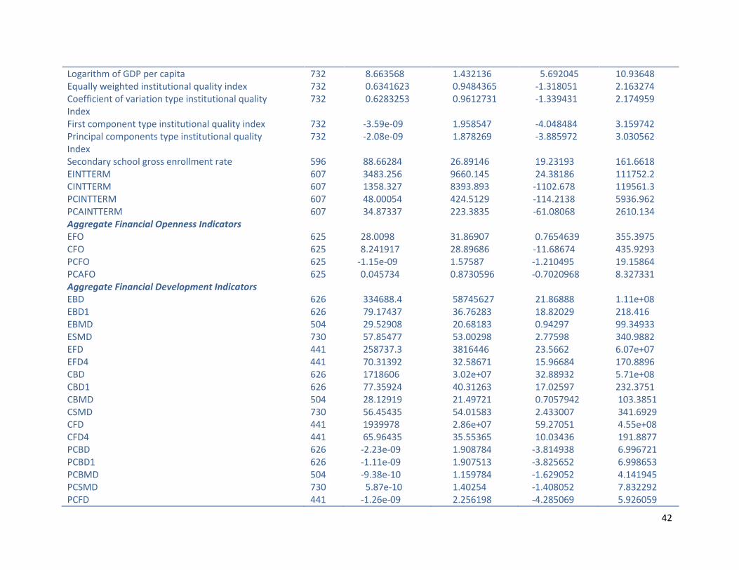
42
Logarithm of GDP per capita 732 8.663568 1.432136 5.692045 10.93648 Equally weighted institutional quality index 732 0.6341623 0.9484365 -1.318051 2.163274 Coefficient of variation type institutional quality Index
732 0.6283253 0.9612731 -1.339431 2.174959
First component type institutional quality index 732 -3.59e-09 1.958547 -4.048484 3.159742 Principal components type institutional quality Index
732 -2.08e-09 1.878269 -3.885972 3.030562
Secondary school gross enrollment rate 596 88.66284 26.89146 19.23193 161.6618 EINTTERM 607 3483.256 9660.145 24.38186 111752.2 CINTTERM 607 1358.327 8393.893 -1102.678 119561.3 PCINTTERM 607 48.00054 424.5129 -114.2138 5936.962 PCAINTTERM 607 34.87337 223.3835 -61.08068 2610.134 Aggregate Financial Openness Indicators EFO 625 28.0098 31.86907 0.7654639 355.3975 CFO 625 8.241917 28.89686 -11.68674 435.9293 PCFO 625 -1.15e-09 1.57587 -1.210495 19.15864 PCAFO 625 0.045734 0.8730596 -0.7020968 8.327331 Aggregate Financial Development Indicators EBD 626 334688.4 58745627 21.86888 1.11e+08 EBD1 626 79.17437 36.76283 18.82029 218.416 EBMD 504 29.52908 20.68183 0.94297 99.34933 ESMD 730 57.85477 53.00298 2.77598 340.9882 EFD 441 258737.3 3816446 23.5662 6.07e+07 EFD4 441 70.31392 32.58671 15.96684 170.8896 CBD 626 1718606 3.02e+07 32.88932 5.71e+08 CBD1 626 77.35924 40.31263 17.02597 232.3751 CBMD 504 28.12919 21.49721 0.7057942 103.3851 CSMD 730 56.45435 54.01583 2.433007 341.6929 CFD 441 1939978 2.86e+07 59.27051 4.55e+08 CFD4 441 65.96435 35.55365 10.03436 191.8877 PCBD 626 -2.23e-09 1.908784 -3.814938 6.996721 PCBD1 626 -1.11e-09 1.907513 -3.825652 6.998653 PCBMD 504 -9.38e-10 1.159784 -1.629052 4.141945 PCSMD 730 5.87e-10 1.40254 -1.408052 7.832292 PCFD 441 -1.26e-09 2.256198 -4.285069 5.926059

43
PCFD4 441 -1.26e-09 2.254396 -4.29558 5.926441 PCABD 626 -0.0640462 1.103597 -3.124777 3.57485 PCABD1 626 -0.0768389 1.303059 -3.447167 4.338953 PCABMD 504 -1.58e-09 0.8237887 -0.975333 3.208189 PCASMD 730 0.0006213 0.9618987 -0.9404376 5.754432 PCAFD 441 0.2059946 1.015499 -2.031706 3.105923 PCAFD4 441 0.2194182 1.141676 -1.944969 3.345601 Notes: The data above is for the period of 1996 – 2007. The countries used in this analysis are as follows: Argentina, Australia, Austria, Belgium, Bangladesh, Brazil, Barbados, Botswana, Canada, Switzerland, Chile, China, Cote d’Ivoire, Colombia, Cyprus, Germany, Denmark, Egypt, Spain, Finland, France, U.K., Ghana, Greece, Hong Kong, Hungary, Indonesia, India, Israel, Italy, Jamaica, Jordan, Japan, Kenya, Republic of Korea, Sri Lanka, Luxembourg, Morocco, Mexico, Mauritius, Malaysia, Nigeria, Netherlands, Norway, New Zealand, Pakistan, Peru, Philippines, Poland, Portugal, Russian Federation, Saudi Arabia, Singapore, Sweden, Thailand, Trinidad and Tobago, Tunisia, Turkey, U.S., Venezuela, South Africa. EFO = Equally weighted financial openness index, EBD = Equally weighted banking development index, EBMD = Equally weighted bond market development index, ESMD = Equally weighted stock market development index, EFD = Equally weighted financial development index, EFD4 = Equally weighted financial development index that excludes the deposit money bank assets to central bank assets ratio, EINTTERM = Equally weighted interaction term between financial and trade openness, CBD = Coefficient of variation type banking sector development index, CBD1 = Coefficient of variation type banking sector development index that excludes the deposit money banks to central bank assets ratio, CBMD = Coefficient of variation type bond market development index, CSMD = Coefficient of variation type stock market development index, CFD = Coefficient of variation type financial development index, CFD4 = Coefficient of variation type financial development index that excludes the deposit money bank assets to central bank assets ratio, CINTTERM = Coefficient of variation type interaction term between financial and trade openness, PCFO = First component financial openness index, PCBD = First component banking sector development index, PCBD1 = First component banking sector development index that excludes the deposit money banks to central bank assets ratio, PCBMD = First component bond market development index, PCSMD = First component stock market development index, PCFD = First component financial development index, PCFD4 = First component financial development index that excludes the deposit money bank assets to central bank assets ratio, PCINTTERM = First component interaction term between financial and trade openness, PCAFO = Principal components financial openness index, PCABD = Principal components banking sector development index, PCABD1 = Principal components banking sector development index that excludes the deposit money banks to central bank assets ratio, PCABMD = Principal components bond market development index, PCASMD = Principal components stock market development index, PCAFD = Principal components financial development index, PCAFD4 = Principal components financial development index that excludes the deposit money bank assets to central bank assets ratio, PCAINTTERM = Principal components interaction term between financial and trade openness.
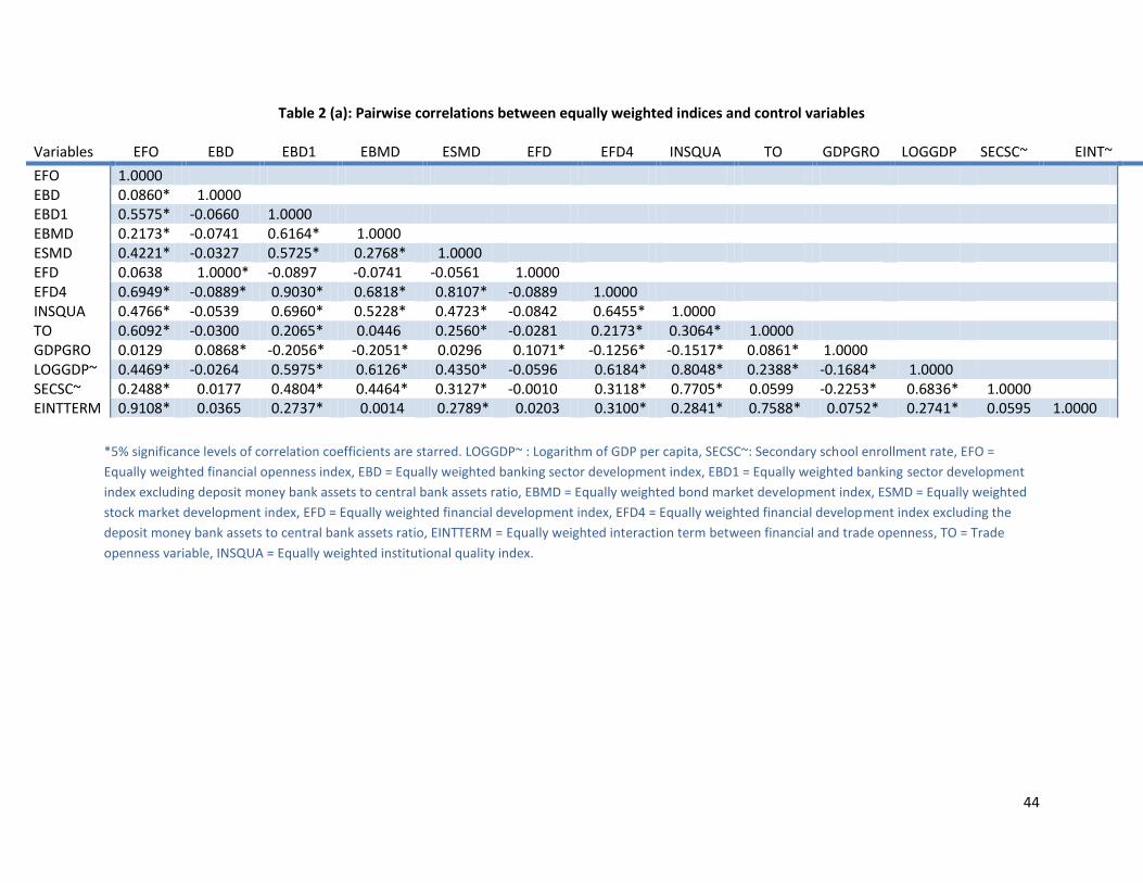
44
Table 2 (a): Pairwise correlations between equally weighted indices and control variables
Variables EFO EBD EBD1 EBMD ESMD EFD EFD4 INSQUA TO GDPGRO LOGGDP SECSC~ EINT~
EFO 1.0000 EBD 0.0860* 1.0000 EBD1 0.5575* -0.0660 1.0000 EBMD 0.2173* -0.0741 0.6164* 1.0000 ESMD 0.4221* -0.0327 0.5725* 0.2768* 1.0000 EFD 0.0638 1.0000* -0.0897 -0.0741 -0.0561 1.0000 EFD4 0.6949* -0.0889* 0.9030* 0.6818* 0.8107* -0.0889 1.0000 INSQUA 0.4766* -0.0539 0.6960* 0.5228* 0.4723* -0.0842 0.6455* 1.0000 TO 0.6092* -0.0300 0.2065* 0.0446 0.2560* -0.0281 0.2173* 0.3064* 1.0000 GDPGRO 0.0129 0.0868* -0.2056* -0.2051* 0.0296 0.1071* -0.1256* -0.1517* 0.0861* 1.0000 LOGGDP~ 0.4469* -0.0264 0.5975* 0.6126* 0.4350* -0.0596 0.6184* 0.8048* 0.2388* -0.1684* 1.0000 SECSC~ 0.2488* 0.0177 0.4804* 0.4464* 0.3127* -0.0010 0.3118* 0.7705* 0.0599 -0.2253* 0.6836* 1.0000 EINTTERM 0.9108* 0.0365 0.2737* 0.0014 0.2789* 0.0203 0.3100* 0.2841* 0.7588* 0.0752* 0.2741* 0.0595 1.0000
*5% significance levels of correlation coefficients are starred. LOGGDP~ : Logarithm of GDP per capita, SECSC~: Secondary school enrollment rate, EFO =
Equally weighted financial openness index, EBD = Equally weighted banking sector development index, EBD1 = Equally weighted banking sector development
index excluding deposit money bank assets to central bank assets ratio, EBMD = Equally weighted bond market development index, ESMD = Equally weighted
stock market development index, EFD = Equally weighted financial development index, EFD4 = Equally weighted financial development index excluding the
deposit money bank assets to central bank assets ratio, EINTTERM = Equally weighted interaction term between financial and trade openness, TO = Trade
openness variable, INSQUA = Equally weighted institutional quality index.

45
Table 2 (b): Pairwise correlations between coefficient of variation type indices and control variables
Variables CFO CBD CBD1 CBMD CSMD CFD CFD4 CINSQUA TO GDPGRO LOGGDP SECSC~ CINTTERM
CFO 1.0000 CBD 0.0247 1.0000 CBD1 0.2656* -0.0680 1.0000 CBMD 0.2172* -0.0689 0.6250* 1.0000 CSMD 0.0480* -0.0343 0.5651* 0.3239* 1.0000 CFD 0.0037 1.0000* -0.0913* -0.0689 -0.0577 1.0000 CFD4 0.4875* -0.0846* 0.8218* 0.6491* 0.8924* -0.0846* 1.0000 CINSQUA 0.2007* -0.0546 0.6900* 0.5518* 0.4613* -0.0847 0.6056* 1.0000 TO 0.3681* -0.0300 0.2075 0.0584 0.2289* -0.0281 0.1951* 0.3026* 1.0000 GDPGRO 0.0206 0.0868* -0.2074* -0.2082* 0.0278 0.1071* -0.0832* -0.1510* 0.0861* 1.0000 LOGGDP~ 0.2095* -0.0264 0.5950* 0.6289* 0.4306* -0.0596 0.5777* 0.8041* 0.2388* -0.1684* 1.0000 SECSC~ 0.0793* 0.0177 0.4695* 0.4481* 0.3076* -0.0010 0.2740* 0.7693* 0.0599 -0.2253* 0.6836* 1.0000 CINTTERM 0.9894* 0.0181 0.1517 0.0345 0.0278 0.0073 0.2567* 0.1637* 0.4097* 0.0368 0.1771* 0.0332 1.0000
*5% significance levels of correlation coefficients are starred. LOGGDP~ : Logarithm of GDP per capita, SECSC~: Secondary school enrollment rate, CFO =
Coefficient of variation type financial openness index, CBD = Coefficient of variation type banking sector development index, CBD1 = Coefficient of variation
type banking sector development index excluding deposit money bank assets to central bank assets ratio, CBMD = Coefficient of variation type bond market
development index, CSMD = Coefficient of variation type stock market development index, CFD = Coefficient of variation type financial development index,
CFD4 = Coefficient of variation type financial development index excluding the deposit money bank assets to central bank assets ratio, CINTTERM = Coefficient
of variation type interaction term between financial and trade openness, TO = Trade openness variable, CINSQUA = Coefficient of variation type institutional
quality index.
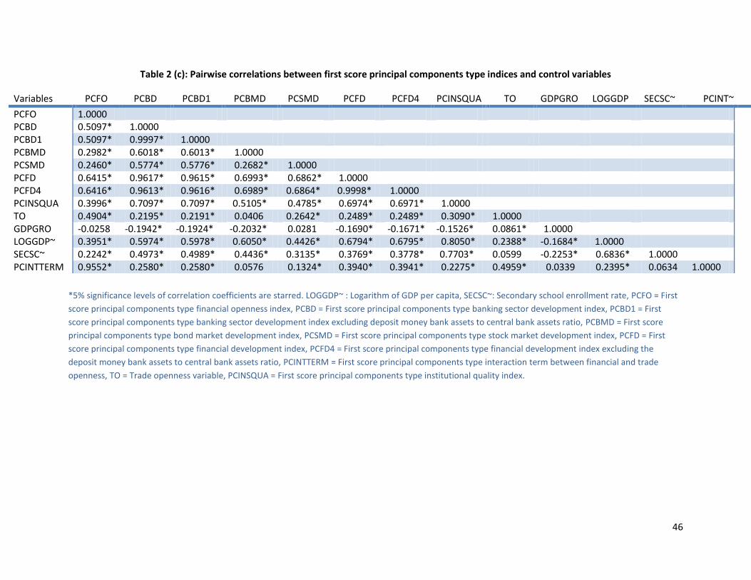
46
Table 2 (c): Pairwise correlations between first score principal components type indices and control variables
Variables PCFO PCBD PCBD1 PCBMD PCSMD PCFD PCFD4 PCINSQUA TO GDPGRO LOGGDP SECSC~ PCINT~
PCFO 1.0000 PCBD 0.5097* 1.0000 PCBD1 0.5097* 0.9997* 1.0000 PCBMD 0.2982* 0.6018* 0.6013* 1.0000 PCSMD 0.2460* 0.5774* 0.5776* 0.2682* 1.0000 PCFD 0.6415* 0.9617* 0.9615* 0.6993* 0.6862* 1.0000 PCFD4 0.6416* 0.9613* 0.9616* 0.6989* 0.6864* 0.9998* 1.0000 PCINSQUA 0.3996* 0.7097* 0.7097* 0.5105* 0.4785* 0.6974* 0.6971* 1.0000 TO 0.4904* 0.2195* 0.2191* 0.0406 0.2642* 0.2489* 0.2489* 0.3090* 1.0000 GDPGRO -0.0258 -0.1942* -0.1924* -0.2032* 0.0281 -0.1690* -0.1671* -0.1526* 0.0861* 1.0000 LOGGDP~ 0.3951* 0.5974* 0.5978* 0.6050* 0.4426* 0.6794* 0.6795* 0.8050* 0.2388* -0.1684* 1.0000 SECSC~ 0.2242* 0.4973* 0.4989* 0.4436* 0.3135* 0.3769* 0.3778* 0.7703* 0.0599 -0.2253* 0.6836* 1.0000 PCINTTERM 0.9552* 0.2580* 0.2580* 0.0576 0.1324* 0.3940* 0.3941* 0.2275* 0.4959* 0.0339 0.2395* 0.0634 1.0000
*5% significance levels of correlation coefficients are starred. LOGGDP~ : Logarithm of GDP per capita, SECSC~: Secondary school enrollment rate, PCFO = First
score principal components type financial openness index, PCBD = First score principal components type banking sector development index, PCBD1 = First
score principal components type banking sector development index excluding deposit money bank assets to central bank assets ratio, PCBMD = First score
principal components type bond market development index, PCSMD = First score principal components type stock market development index, PCFD = First
score principal components type financial development index, PCFD4 = First score principal components type financial development index excluding the
deposit money bank assets to central bank assets ratio, PCINTTERM = First score principal components type interaction term between financial and trade
openness, TO = Trade openness variable, PCINSQUA = First score principal components type institutional quality index.

47
Table 2 (d): Pairwise correlations between principal components (new methodology) type indices and control variables
Variables PCAFO PCABD PCABD1 PCABMD PCASMD PCAFD PCAFD4 PCAINSQUA TO GDPGRO LOGGDP SECSC~ PCAINTTERM
PCAFO 1.0000 PCABD 0.5672* 1.0000 PCABD1 0.5662* 0.9957* 1.0000 PCABMD 0.2679* 0.6039* 0.6110* 1.0000 PCASMD 0.2243* 0.4863* 0.4912* 0.3336* 1.0000 PCAFD 0.6694* 0.9292* 0.9231* 0.6962* 0.6749* 1.0000 PCAFD4 0.6347* 0.8827* 0.8912* 0.7783* 0.7054* 0.9798* 1.0000 PCAINSQUA 0.5189* 0.7224* 0.7243* 0.5584* 0.3946* 0.6845* 0.6761* 1.0000 TO 0.6209* 0.2129* 0.2162* 0.0668 0.1072* 0.2320* 0.2052* 0.3097* 1.0000 GDPGRO -0.0098 -0.1579* -0.1712* -0.2071* 0.0270 -0.1182* -0.1370* -0.1529* 0.0861* 1.0000 LOGGDP~ 0.4762* 0.5871* 0.5921* 0.6299* 0.3742* 0.6570* 0.6711* 0.8050* 0.2388* -0.1684* 1.0000 SECSC~ 0.2917* 0.5354* 0.5271* 0.4419* 0.2792* 0.3676* 0.3644* 0.7701* 0.0599 -0.2253* 0.6836* 1.0000 PCAINTTERM 0.9069* 0.2738* 0.2736* 0.0206 0.1285* 0.3048* 0.2784* 0.2862* 0.6922* 0.0613 0.2817* 0.0641 1.0000
*5% significance levels of correlation coefficients are starred. LOGGDP~ : Logarithm of GDP per capita, SECSC~: Secondary school enrollment rate, PCAFO =
Principal components type financial openness index, PCABD = Principal components type banking sector development index, PCABD1 = Principal components
type banking sector development index excluding deposit money bank assets to central bank assets ratio, PCABMD = Principal components type bond market
development index, PCASMD = Principal components type stock market development index, PCAFD = Principal components type financial development index,
PCAFD4 = Principal components type financial development index excluding the deposit money bank assets to central bank assets ratio, PCAINTTERM =
Principal components type interaction term between financial and trade openness, TO = Trade openness variable, PCAINSQUA = Principal components type
institutional quality index.
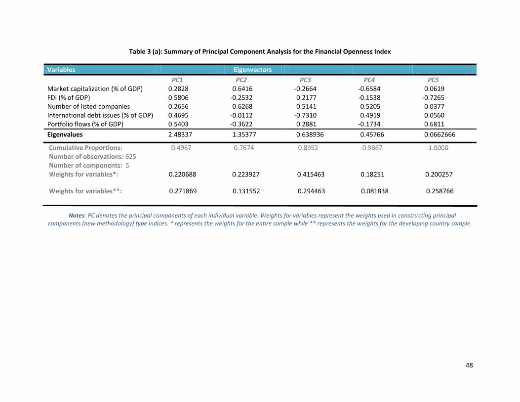
48
Table 3 (a): Summary of Principal Component Analysis for the Financial Openness Index
Variables Eigenvectors
PC1 PC2 PC3 PC4 PC5 Market capitalization (% of GDP) 0.2828 0.6416 -0.2664 -0.6584 0.0619 FDI (% of GDP) 0.5806 -0.2532 0.2177 -0.1538 -0.7265 Number of listed companies 0.2656 0.6268 0.5141 0.5205 0.0377 International debt issues (% of GDP) 0.4695 -0.0112 -0.7310 0.4919 0.0560 Portfolio flows (% of GDP) 0.5403 -0.3622 0.2881 -0.1734 0.6811
Eigenvalues 2.48337 1.35377 0.638936 0.45766 0.0662666
Cumulative Proportions: 0.4967 0.7674 0.8952 0.9867 1.0000 Number of observations: 625 Number of components: 5 Weights for variables*: 0.220688 0.223927 0.415463 0.18251 0.200257
Weights for variables**: 0.271869 0.131552 0.294463 0.081838 0.258766
Notes: PC denotes the principal components of each individual variable. Weights for variables represent the weights used in constructing principal
components (new methodology) type indices. * represents the weights for the entire sample while ** represents the weights for the developing country sample.

49
Table 3 (b): Summary of Principal Component Analysis for the Banking Sector Development Index
Variables Eigenvectors
PC1 PC2 PC3 PC4 PC5 PC6 Liquid liabilities (% of GDP) 0.4524 -0.0280 -0.1863 0.7825 0.2998 -0.2400 Private credit (% of GDP) 0.4871 0.0244 0.0384 -0.5171 0.0825 -0.6975 Deposit money bank~ 0.2789 0.3251 0.8802 0.1222 -0.0345 0.1599 Total bank assets (% of GDP) 0.4890 -0.0550 -0.2089 0.0411 -0.8199 0.2006 Deposit money bank assets~ -0.0428 0.9422 -0.3317 -0.0189 -0.0056 -0.0019 Domestic credit (% of GDP) 0.4892 -0.0463 -0.1880 -0.3214 0.4794 0.6246
Eigenvalues 3.64346 1.02264 0.775641 0.342712 0.130448 0.0851036
Cumulative Proportions: 0.6072 0.7777 0.9070 0.9641 0.9858 1.0000 Number of observations: 626 Number of components: 6 Weights for variables*: 0.29367 0.267275 0.347055 0.24793 0.09049 0.265793
Weights for variables**: 0.330091 0.268812 0.132193 0.316745 0.200221 0.290658
Notes: PC denotes the principal components of each individual variable. Deposit money bank~: Deposit money bank assets to the sum of central bank
assets and deposit money bank assets, Deposit money bank assets~: Deposit money bank assets to central bank assets ratio. Weights for variables represent the weights used in constructing principal components (new methodology) type indices. * represents the weights for the entire sample while ** represents the
weights for the developing country sample.
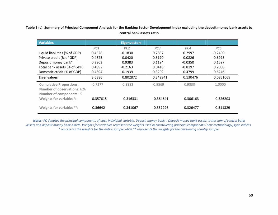
50
Table 3 (c): Summary of Principal Component Analysis for the Banking Sector Development Index excluding the deposit money bank assets to
central bank assets ratio
Variables Eigenvectors
PC1 PC2 PC3 PC4 PC5 Liquid liabilities (% of GDP) 0.4528 -0.1830 0.7837 0.2997 -0.2400 Private credit (% of GDP) 0.4875 0.0420 -0.5170 0.0826 -0.6975 Deposit money bank~ 0.2803 0.9383 0.1194 -0.0350 0.1597 Total bank assets (% of GDP) 0.4892 -0.2163 0.0418 -0.8197 0.2008 Domestic credit (% of GDP) 0.4894 -0.1939 -0.3202 0.4799 0.6246
Eigenvalues 3.6386 0.802872 0.342941 0.130476 0.0851069
Cumulative Proportions: 0.7277 0.8883 0.9569 0.9830 1.0000 Number of observations: 626 Number of components: 5 Weights for variables*: 0.357615 0.316331 0.364641 0.306163 0.326203
Weights for variables**: 0.36642 0.341067 0.337296 0.326477 0.311329
Notes: PC denotes the principal components of each individual variable. Deposit money bank~: Deposit money bank assets to the sum of central bank
assets and deposit money bank assets. Weights for variables represent the weights used in constructing principal components (new methodology) type indices. * represents the weights for the entire sample while ** represents the weights for the developing country sample.

51
Table 3 (d): Summary of Principal Component Analysis for the Bond Market Development Index
Variables Eigenvectors
PC1 PC2 Private bond market capitalization (% of GDP) 0.7071 0.7071 Public bond market capitalization (% of GDP) 0.7071 - 0.7071
Eigenvalues 1.3451 0.6549
Cumulative Proportions: 0.6726 1.0000 Number of observations: 504 Number of components: 2 Weights for variables*: 0.7071 0.24402
Weights for variables**: 0.707099 0.150402
Notes: PC denotes the principal components of each individual variable. Weights for
variables represent the weights used in constructing principal components (new methodology) type indices.* represents the weights for the entire sample while ** represents the weights
for the developing country sample.
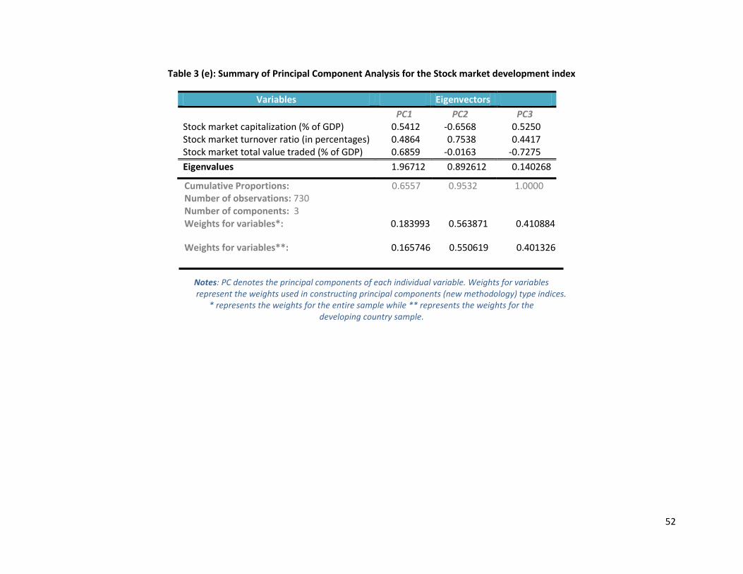
52
Table 3 (e): Summary of Principal Component Analysis for the Stock market development index
Variables Eigenvectors
PC1 PC2 PC3 Stock market capitalization (% of GDP) 0.5412 -0.6568 0.5250 Stock market turnover ratio (in percentages) 0.4864 0.7538 0.4417 Stock market total value traded (% of GDP) 0.6859 -0.0163 -0.7275
Eigenvalues 1.96712 0.892612 0.140268
Cumulative Proportions: 0.6557 0.9532 1.0000 Number of observations: 730 Number of components: 3 Weights for variables*: 0.183993 0.563871 0.410884
Weights for variables**: 0.165746 0.550619 0.401326
Notes: PC denotes the principal components of each individual variable. Weights for variables
represent the weights used in constructing principal components (new methodology) type indices. * represents the weights for the entire sample while ** represents the weights for the
developing country sample.

53
Table 3 (f): Summary of Principal Component Analysis for the Financial Development Index
Variables Eigenvectors
PC1 PC2 PC3 PC4 PC5 PC6 PC7 PC8 PC9 PC10 PC11 Liquid liabilities (% of GDP)
0.3718 -0.2705 -0.0363 0.0112 -0.2036 0.3889 0.0114 0.3803 -0.0615 0.5545 -0.3721
Private credit (% of GDP) 0.4101 0.0209 0.1146 -0.0949 0.1025 0.0289 -0.2748 -0.4908 -0.0907 -0.3157 -0.6112 Deposit money bank~ 0.2234 0.0038 0.4272 -0.0595 0.7073 0.1635 0.4636 -0.0007 -0.0257 0.0912 0.1145 Total bank assets (% of GDP)
0.3869 -0.2454 -0.0003 -0.0335 -0.0330 0.3030 -0.1948 0.3405 0.3191 -0.5761 0.3295
Deposit money bank assets~
-0.0445 0.0402 0.5679 0.7864 -0.2007 0.0516 -0.1076 -0.0134 -0.0043 -0.0288 -0.0008
Domestic credit (% of GDP)
0.4090 -0.1744 -0.0610 0.0255 -0.1109 -0.0142 -0.1836 -0.4797 -0.2899 0.3012 0.5890
Private bond market~ 0.3023 0.0789 -0.0799 0.1648 0.3535 -0.6518 -0.3842 0.3353 0.1465 0.1922 -0.0241 Public bond market~ 0.2015 -0.3801 -0.3985 0.3935 -0.0630 -0.2891 0.5912 -0.1056 0.0211 -0.1941 -0.1218 Stock market~ 0.2908 0.2667 0.3129 -0.2727 -0.4441 -0.2589 0.3000 -0.1144 0.5355 0.1305 0.0286 Stock market turnover~ 0.1222 0.5648 -0.4614 0.3325 0.1683 0.3840 -0.0008 -0.1700 0.3486 0.1248 0.0302 Stock total value traded~
0.3054 0.5415 -0.0285 -0.0159 -0.1989 -0.0600 0.1977 0.3205 -0.6093 -0.2320 0.0485
Eigenvalues 5.09043 1.35958 1.1467 0.934689 0.775953 0.672766 0.584361 0.16068 0.127049 0.10182 0.04597 Cumulative Proportions:
0.4628
0.5864
0.6906
0.7756
0.8461
0.9073
0.9604
0.9750
0.9866
0.9958
1.0000
Num. of obs.: 441 Num. of components: 11 Weights for variables*: Weights for variables**:
0.154240.21694
0.1769530.163011
0.22886700.074862
0.15639500.193194
0.0931650.083358
0.13997300.176872
0.1282500.181118
0.043830.13584
0.1515990.14052
0.144650.15856
0.192430.18567
Notes: PC denotes the principal components of each individual variable. Deposit money bank~: Deposit money bank assets to the sum of central bank assets and deposit money
bank assets, Deposit money bank assets~: Deposit money bank assets to central bank assets ratio, Private bond market~: Private bond market capitalization (% of GDP), Public
bond market~: Public bond market capitalization (% of GDP), Stock market~: Stock market capitalization (% of GDP), Stock market turnover ratio (in percentages), Stock total
value traded~: Stock market total value traded (% of GDP). Weights for variables represent the weights used in constructing principal components (new methodology) type
indices. * represents the weights for the entire sample while ** represents the weights for the developing country sample.

54
Table 3 (g): Summary of Principal Component Analysis for the Financial Development Index excluding deposit money
bank assets to central bank assets ratio
Variables Eigenvectors
PC1 PC2 PC3 PC4 PC5 PC6 PC7 PC8 PC9 PC10 Liquid liabilities (% of GDP)
0.3720 -0.2704 0.0570 -0.2052 -0.3816 0.0306 0.3840 -0.0594 0.5541 -0.3722
Private credit (% of GDP) 0.4104 0.0189 -0.1464 0.0798 -0.0399 -0.2824 -0.4926 -0.0913 -0.3125 -0.6110 Deposit money bank~ 0.2246 -0.0059 -0.4402 0.7114 -0.1708 0.4460 -0.0019 -0.0258 0.0882 0.1144 Total bank assets (% of GDP)
0.3870 -0.2453 -0.0032 -0.0503 -0.3072 -0.1891 0.3383 0.3163 -0.5781 0.3297
Domestic credit (% of GDP)
0.4092 -0.1736 0.0789 -0.1110 0.0140 -0.1785 -0.4777 -0.2876 0.3067 0.5889
Private bond market~ 0.3026 0.0792 0.1332 0.3788 0.6392 -0.4006 0.3369 0.1469 0.1904 -0.0242 Public bond market~ 0.2013 -0.3744 0.5442 0.0120 0.3120 0.6014 -0.1066 0.0204 -0.1935 -0.1217 Stock market~ 0.2916 0.2609 -0.3952 -0.4584 0.2710 0.2995 -0.1135 0.5361 0.1278 0.0285 Stock market turnover~ 0.1218 0.5728 0.5523 0.1992 -0.3808 0.0146 -0.1680 0.3496 0.1258 0.0302 Stock total value traded~
0.3058 0.5418 0.0157 -0.1927 0.0687 -0.2016 0.3182 -0.6108 -0.2312 0.0485
Eigenvalues 5.0823 1.35905 1.07573 0.784147 0.673569 0.588792 0.160829 0.12706 0.102543 0.04597 Cumulative Proportions: 0.5082 0.6441 0.7517 0.8301 0.8975 0.9564 0.9724 0.9851 0.9954 1.0000
Num. of obs.: 441 Num. of components: 10 Weights for variables*: Weights for variables**:
0.12784
0.18507
0.167244
0.191976
0.137605
0.183899
0.13228
0.16247
0.169106
0.19464
0.23718
0.161879
0.163332
0.155323
0.14751
0.20263
0.193161
0.12997
0.22733
0.23771
Notes: PC denotes the principal components of each individual variable. Deposit money bank~: Deposit money bank assets to the sum of central bank assets and deposit money bank assets, Private bond market~: Private bond market capitalization (% of GDP), Public bond market~: Public bond market capitalization (% of GDP), Stock market~: Stock market capitalization (% of GDP), Stock market turnover ratio (in percentages), Stock total value traded~: Stock market total value traded (% of GDP). Weights for variables
represent the weights used in constructing principal components (new methodology) type indices. * represents the weights for the entire sample while ** represents the weights for the developing country sample.

55
Table 3 (h): Summary of Principal Component Analysis for the Institutional Quality Index
Variables Eigenvectors
PC1 PC2 PC3 PC4 Government effectiveness 0.5021 -0.2055 -0.7095 0.4498 Regulatory quality 0.4935 0.8576 0.1347 0.0533 Rule of law 0.5003 -0.4158 0.6839 0.3303 Control of corruption 0.5041 -0.2223 -0.1039 -0.8281
Eigenvalues 3.8359 0.0882176 0.0458957 0.0458957
Cumulative Proportions: 0.9590 0.9810 0.9925 1.0000 Number of observations: 732 Number of components: 4 Weights for variables*: 0.4722 0.494113 0.480928 0.471117
Weights for variables**: 0.432668 0.490725 0.43863 0.424311
Notes: PC denotes the principal components of each individual variable. Weights for variables represent the weights used in constructing principal components (new methodology) type indices. * represents the weights for the entire sample while ** represents the weights for the developing country sample.
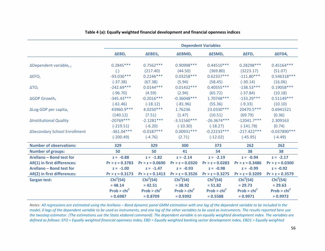
56
Table 4 (a): Equally weighted financial development and financial openness indices
Dependent Variables
∆EBDt ∆EBD1t ∆EBMDt ∆ESMDt ∆EFDt ∆EFD4t
∆Dependent variablet-1 0.2845*** (.)
0.7562*** (217.40)
0.90998*** (44.50)
0.44510*** (369.80)
0.28298*** (3223.17)
0.45164*** (51.07)
∆EFOt -93.036*** (-37.38)
0.2246*** (67.38)
0.03258*** (5.94)
0.62337*** (58.45)
-111.80*** (-30.14)
0.546318*** (16.06)
∆TOt -242.69*** (-96.70)
0.0144*** (4.59)
0.01432*** (2.94)
0.40555*** (65.72)
-138.53*** (-37.84)
0.19058*** (10.18)
∆GDP Growtht -345.43*** (-61.46)
-0.2016*** (-18.12)
-0.36048*** (-81.96)
1.70748*** (55.36)
-133.29*** (-9.33)
0.51149*** (10.10)
∆Log GDP per capitat 43960.9*** (140.12)
4.0250*** (7.51)
1.76236 (1.47)
23.0330*** (10.51)
20470.5*** (69.79)
0.6941521 (0.36)
∆Institutional Quality -20769*** (-219.51)
-2.1281*** (-6.20)
-3.51560*** (-10.30)
-26.3674*** (-18.27)
-12041.7*** (-141.78)
2.309163 (0.74)
∆Secondary School Enrollment -361.04*** (-200.49)
-0.0187*** (-4.76)
0.00931*** (2.71)
-0.22233*** (-12.02)
-217.422*** (-45.95)
-0.037890*** (-4.49)
Number of observations: 329 329 300 373 262 262
Number of groups: 50 50 41 54 38 38
Arellano – Bond test for AR(1) in first differences: Arellano – Bond test for AR(2) in first differences:
z = -0.88 Pr > z = 0.3783 z = -1.00 Pr > z = 0.3173
z = -1.82 Pr > z = 0.0690 z = -1.47 Pr > z = 0.1413
z = -2.14 Pr > z = 0.0320 z = -0.93 Pr > z = 0.3526
z = -2.19 Pr > z = 0.0283 z = -0.98 Pr > z = 0.3275
z = -0.94 Pr > z = 0.3486 z = -0.99 Pr > z = 0.3209
z = -2.17 Pr > z = 0.0300 z = -0.92 Pr > z = 0.3579
Sargan test: Chi2(54) = 48.14 Prob > chi2 = 0.6987
Chi2(54) = 42.51 Prob > chi2 = 0.8709
Chi2(54) = 38.92 Prob > chi2 = 0.9392
Chi2(54) = 51.82 Prob > chi2 = 0.5588
Chi2(54) = 29.73 Prob > chi2 = 0.9971
Chi2(54) = 29.63 Prob > chi2 = 0.9972
Notes: All regressions are estimated using the Arellano – Bond dynamic panel GMM estimation with one lag of the dependent variable to be included in the model, 0 lags of the dependent variable to be used as instruments, and one lag of the other variables to be used as instruments. The results reported here use the twostep estimator. (The estimations use the Stata xtabond command). The dependent variable is an equally weighted development index. The variables are defined as follows: EFO = Equally weighted financial openness index, EBD = Equally weighted banking sector development index, EBD1 = Equally weighted

57
banking sector development index that excludes the deposit money banks to central bank assets ratio, EBMD = Equally weighted bond market development index, ESMD = Equally weighted stock market development index, EFD = Equally weighted financial development index, EFD4 = Equally weighted financial development index that excludes the deposit money bank assets to central bank assets ratio. Institutional quality index is constructed using the equally weighted indexing procedure. Figures in brackets are t-statistics and the stars represent the significant t statistics for 1%, 5%, and 10% confidence levels respectively.

58
Table 4 (b): Coefficient of variation type financial development and financial openness indices
Dependent Variables
∆CBDt ∆CBD1t ∆CBMDt ∆CSMDt ∆CFDt ∆CFD4t
∆Dependent variablet-1 0.28745*** (.)
0.80089*** (128.23)
0.89815*** (64.59)
0.43401*** (416.73)
0.28804*** (5485.95)
0.36762*** (33.80)
∆CFOt -155.89*** (-28.46)
0.09445*** (24.13)
-0.01544** (-2.36)
0.13981*** (14.19)
293.114*** (23.20)
0.95850*** (34.59)
∆TOt -1405.6*** (-215.79)
0.07587*** (13.16)
0.03514*** (6.25)
0.70369*** (83.77)
-1410.37*** (-138.69)
0.46417*** (24.83)
∆GDP Growtht -1712.1*** (-73.53)
-0.24926*** (-13.71)
-0.34054*** (-68.66)
1.75160*** (48.57)
-1127.96*** (-26.13)
0.77060*** (8.29)
∆Log GDP per capitat 208992*** (327.17)
12.2716*** (13.21)
2.79637** (2.21)
35.8328*** (17.16)
132876*** (125.59)
8.71828*** (4.64)
∆C Institutional Quality -111119*** (-149.64)
-4.6047*** (-13.35)
-4.66715*** (-19.18)
-33.5282*** (-41.08)
-96394.6*** (-166.34)
-13.1181*** (-3.50)
∆Secondary School Enrollment -1820.87*** (-323.71)
-0.0530*** (-5.88)
-0.00227 (-1.09)
-0.264363*** (-15.80)
-1693.067*** (-118.65)
-0.143120*** (-8.18)
Number of observations: 329 329 300 373 262 262
Number of groups: 50 50 41 54 38 38
Arellano – Bond test for AR(1) in first differences: Arellano – Bond test for AR(2) in first differences:
z = -0.88 Pr > z = 0.3798 z = -1.00 Pr > z = 0.3176
z = -1.86 Pr > z =0.0625 z = -1.30 Pr > z =0.1928
z = -2.47 Pr > z = 0.0136 z = -1.26 Pr > z =0.2088
z = -2.22 Pr > z =0.0266 z = -0.84 Pr > z=0.4033
z = -0.91 Pr > z=0.3625 z = -0.99 Pr > z=0.3204
z = -2.13 Pr > z=0.0333 z = -1.20 Pr > z=0.2304
Sargan test: Chi2(54) = 46.60 Prob > chi2 = 0.7524
Chi2(54) = 42.25 Prob > chi2 = 0.8768
Chi2(54) = 37.02 Prob > chi2
= 0.9624
Chi2(54) = 49.98 Prob > chi2 = 0.6300
Chi2(54) = 33.89 Prob > chi2 = 0.9854
Chi2(54) = 31.03 Prob > chi2 = 0.9949
Notes: All regressions are estimated using the Arellano – Bond dynamic panel GMM estimation with one lag of the dependent variable to be included in the model, 0 lags of the dependent variable to be used as instruments, and one lag of the other variables to be used as instruments. The results reported here use the twostep estimator. The index measures are constructed using the coefficient of variation methodology. The variables are defined as follows: CFO = Coefficient of variation type financial openness index, CBD = Coefficient of variation type banking sector development index, CBD1 = Coefficient of variation type
59
banking sector development index that excludes the deposit money banks to central bank assets ratio, CBMD = Coefficient of variation type bond market development index, CSMD = Coefficient of variation type stock market development index, CFD = Coefficient of variation type financial development index, CFD4 = Coefficient of variation type financial development index that excludes the deposit money bank assets to central bank assets ratio. Institutional quality index is constructed using the coefficient of variation methodology. Figures in brackets are t-statistics and the stars represent the significant t-statistics for 1%, 5%, and 10% confidence levels respectively.
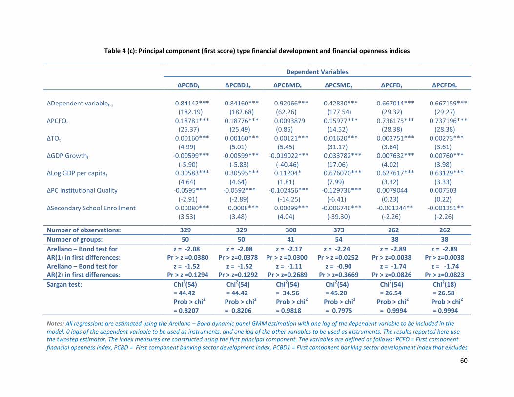
60
Table 4 (c): Principal component (first score) type financial development and financial openness indices
Dependent Variables
∆PCBDt ∆PCBD1t ∆PCBMDt ∆PCSMDt ∆PCFDt ∆PCFD4t
∆Dependent variablet-1 0.84142*** (182.19)
0.84160*** (182.68)
0.92066*** (62.26)
0.42830*** (177.54)
0.667014*** (29.32)
0.667159*** (29.27)
∆PCFOt 0.18781*** (25.37)
0.18776*** (25.49)
0.0093879 (0.85)
0.15977*** (14.52)
0.736175*** (28.38)
0.737196*** (28.38)
∆TOt 0.00160*** (4.99)
0.00160*** (5.01)
0.00121*** (5.45)
0.01620*** (31.17)
0.002751*** (3.64)
0.00273*** (3.61)
∆GDP Growtht -0.00599*** (-5.90)
-0.00599*** (-5.83)
-0.019022*** (-40.46)
0.033782*** (17.06)
0.007632*** (4.02)
0.00760*** (3.98)
∆Log GDP per capitat 0.30583*** (4.64)
0.30595*** (4.64)
0.11204* (1.81)
0.676070*** (7.99)
0.627617*** (3.32)
0.63129*** (3.33)
∆PC Institutional Quality -0.0595*** (-2.91)
-0.0592*** (-2.89)
-0.102456*** (-14.25)
-0.129736*** (-6.41)
0.0079044 (0.23)
0.007503 (0.22)
∆Secondary School Enrollment 0.00080*** (3.53)
0.0008*** (3.48)
0.00099*** (4.04)
-0.006746*** (-39.30)
-0.001244** (-2.26)
-0.001251** (-2.26)
Number of observations: 329 329 300 373 262 262
Number of groups: 50 50 41 54 38 38
Arellano – Bond test for AR(1) in first differences: Arellano – Bond test for AR(2) in first differences:
z = -2.08 Pr > z =0.0380 z = -1.52 Pr > z =0.1294
z = -2.08 Pr > z=0.0378 z = -1.52 Pr > z=0.1292
z = -2.17 Pr > z =0.0300 z = -1.11 Pr > z=0.2689
z = -2.24 Pr > z =0.0252 z = -0.90 Pr > z=0.3669
z = -2.89 Pr > z=0.0038 z = -1.74 Pr > z=0.0826
z = -2.89 Pr > z=0.0038 z = -1.74 Pr > z=0.0823
Sargan test: Chi2(54) = 44.42 Prob > chi2 = 0.8207
Chi2(54) = 44.42 Prob > chi2 = 0.8206
Chi2(54) = 34.56 Prob > chi2
= 0.9818
Chi2(54) = 45.20 Prob > chi2 = 0.7975
Chi2(54) = 26.54 Prob > chi2 = 0.9994
Chi2(18) = 26.58 Prob > chi2 = 0.9994
Notes: All regressions are estimated using the Arellano – Bond dynamic panel GMM estimation with one lag of the dependent variable to be included in the model, 0 lags of the dependent variable to be used as instruments, and one lag of the other variables to be used as instruments. The results reported here use the twostep estimator. The index measures are constructed using the first principal component. The variables are defined as follows: PCFO = First component financial openness index, PCBD = First component banking sector development index, PCBD1 = First component banking sector development index that excludes
61
the deposit money banks to central bank assets ratio, PCBMD = First component bond market development index, PCSMD = First component stock market development index, PCFD = First component financial development index, PCFD4 = First component financial development index that excludes the deposit money bank assets to central bank assets ratio. Institutional quality index is constructed using the first principal component of the individual institutional quality measures. Figures in brackets are t-statistics and the stars represent the significant t-statistics for 1%, 5%, and 10% confidence levels respectively..

62
Table 4 (d): Principal component analysis (new methodology) type financial development and financial openness indices
Dependent Variables
∆PCABDt ∆PCABD1t ∆PCABMDt ∆PCASMDt ∆PCAFDt ∆PCAFD4t
∆Dependent variablet-1 0.86929*** (89.11)
0.871759*** (77.41)
0.84670*** (65.73)
0.304918*** (120.67)
0.60474*** (72.78)
0.44201*** (30.34)
∆PCAFOt 0.16546*** (12.95)
0.204118*** (14.72)
0.11894*** (13.01)
0.255378*** (10.96)
0.73309*** (27.56)
0.85960*** (45.65)
∆TOt 0.000669** (2.26)
0.000651* (1.71)
0.00060*** (4.38)
0.007924*** (42.70)
0.00387*** (15.30)
0.00493*** (11.44)
∆GDP Growtht 0.001170** (2.42)
0.0000948 (0.17)
-0.010550*** (-21.10)
0.033182*** (33.19)
0.01664*** (11.43)
0.01589*** (9.47)
∆Log GDP per capitat 0.08265*** (3.16)
0.09658*** (2.78)
0.0294515 (1.43)
0.138069*** (2.44)
-0.10891* (-1.93)
-0.0490796 (-0.63)
∆PCA Institutional Quality -0.0138673 (-1.35)
-0.025017 (-1.51)
-0.080613*** (-18.02)
-0.136876*** (-10.00)
0.0637*** (4.45)
0.04465*** (3.02)
∆Secondary School Enrollment 0.000656*** (3.17)
0.00074*** (3.00)
-0.000501** (-2.57)
-0.004251*** (-11.52)
-0.0005151 (-1.19)
0.00064** (2.36)
Number of observations: 329 329 300 373 262 262
Number of groups: 50 50 41 54 38 38
Arellano – Bond test for AR(1) in first differences: Arellano – Bond test for AR(2) in first differences:
z = -2.54 Pr > z = 0.0110 z = -1.70 Pr > z = 0.0886
z = -2.45 Pr > z =0.0141 z = -1.66 Pr > z =0.0973
z = -2.28 Pr > z =0.0226 z = -1.31 Pr > z=0.1900
z = -2.00 Pr > z =0.0458 z = -1.00 Pr > z=0.3164
z = -2.51 Pr >z=0.0121 z = -1.02 Pr >z=0.3093
z = -2.27 Pr >z=0.0235 z = -0.97 Pr >z=0.3333
Sargan test: Chi2(54) = 45.51 Prob > chi2 = 0.7878
Chi2(54) = 45.54 Prob > chi2 = 0.7869
Chi2(54) = 34.65 Prob > chi2
= 0.9812
Chi2(54) = 43.86 Prob > chi2 = 0.8362
Chi2(54) = 28.36 Prob > chi2 = 0.9984
Chi2(54) = 31.25 Prob > chi2 = 0.9944
Notes: All regressions are estimated using the Arellano – Bond dynamic panel GMM estimation with one lag of the dependent variable to be included in the model, 0 lags of the dependent variable to be used as instruments, and one lag of the other variables to be used as instruments. The results reported here use the twostep estimator. The index measures are constructed following the principal component methodology that utilizes all components. The variables are defined as follows: PCAFO = Principal components financial openness index, PCABD = Principal components banking sector development index, PCABD1 =

63
Principal components banking sector development index that excludes the deposit money banks to central bank assets ratio, PCABMD = Principal components bond market development index, PCASMD = Principal components stock market development index, PCAFD = Principal components financial development index, PCFD4 = Principal components financial development index that excludes the deposit money bank assets to central bank assets ratio. Institutional quality index is constructed using the principal components methodology. Figures in brackets are t-statistics and the stars represent the significant t-statistics for 1%, 5%, and 10% confidence levels respectively.
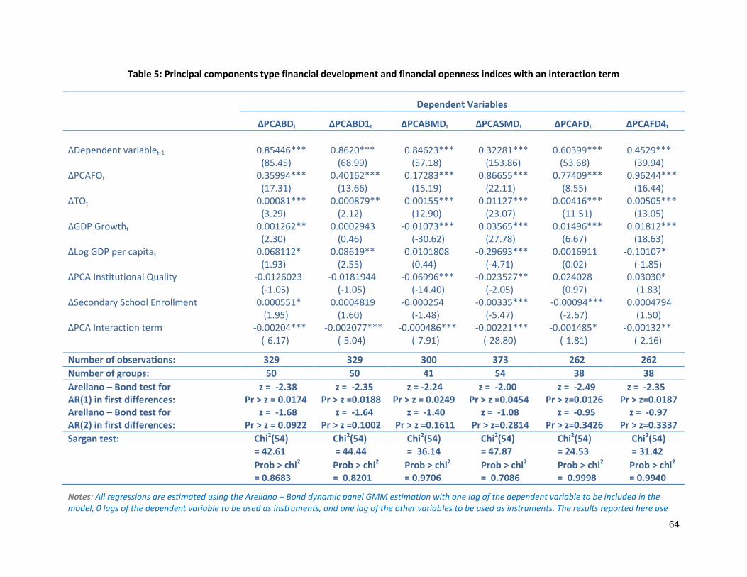
64
Table 5: Principal components type financial development and financial openness indices with an interaction term
Dependent Variables
∆PCABDt ∆PCABD1t ∆PCABMDt ∆PCASMDt ∆PCAFDt ∆PCAFD4t
∆Dependent variablet-1 0.85446*** (85.45)
0.8620*** (68.99)
0.84623*** (57.18)
0.32281*** (153.86)
0.60399*** (53.68)
0.4529*** (39.94)
∆PCAFOt 0.35994*** (17.31)
0.40162*** (13.66)
0.17283*** (15.19)
0.86655*** (22.11)
0.77409*** (8.55)
0.96244*** (16.44)
∆TOt 0.00081*** (3.29)
0.000879** (2.12)
0.00155*** (12.90)
0.01127*** (23.07)
0.00416*** (11.51)
0.00505*** (13.05)
∆GDP Growtht 0.001262** (2.30)
0.0002943 (0.46)
-0.01073*** (-30.62)
0.03565*** (27.78)
0.01496*** (6.67)
0.01812*** (18.63)
∆Log GDP per capitat 0.068112* (1.93)
0.08619** (2.55)
0.0101808 (0.44)
-0.29693*** (-4.71)
0.0016911 (0.02)
-0.10107* (-1.85)
∆PCA Institutional Quality -0.0126023 (-1.05)
-0.0181944 (-1.05)
-0.06996*** (-14.40)
-0.023527** (-2.05)
0.024028 (0.97)
0.03030* (1.83)
∆Secondary School Enrollment 0.000551* (1.95)
0.0004819 (1.60)
-0.000254 (-1.48)
-0.00335*** (-5.47)
-0.00094*** (-2.67)
0.0004794 (1.50)
∆PCA Interaction term -0.00204*** (-6.17)
-0.002077*** (-5.04)
-0.000486*** (-7.91)
-0.00221*** (-28.80)
-0.001485* (-1.81)
-0.00132** (-2.16)
Number of observations: 329 329 300 373 262 262
Number of groups: 50 50 41 54 38 38
Arellano – Bond test for AR(1) in first differences: Arellano – Bond test for AR(2) in first differences:
z = -2.38 Pr > z = 0.0174 z = -1.68 Pr > z = 0.0922
z = -2.35 Pr > z =0.0188 z = -1.64 Pr > z =0.1002
z = -2.24 Pr > z = 0.0249 z = -1.40 Pr > z =0.1611
z = -2.00 Pr > z =0.0454 z = -1.08 Pr > z=0.2814
z = -2.49 Pr > z=0.0126 z = -0.95 Pr > z=0.3426
z = -2.35 Pr > z=0.0187 z = -0.97 Pr > z=0.3337
Sargan test: Chi2(54) = 42.61
Prob > chi2 = 0.8683
Chi2(54) = 44.44
Prob > chi2 = 0.8201
Chi2(54) = 36.14
Prob > chi2
= 0.9706
Chi2(54) = 47.87
Prob > chi2 = 0.7086
Chi2(54) = 24.53
Prob > chi2 = 0.9998
Chi2(54) = 31.42
Prob > chi2 = 0.9940
Notes: All regressions are estimated using the Arellano – Bond dynamic panel GMM estimation with one lag of the dependent variable to be included in the model, 0 lags of the dependent variable to be used as instruments, and one lag of the other variables to be used as instruments. The results reported here use

65
the twostep estimator. The index measures are constructed following the principal component methodology that utilizes all components. The variables are defined as follows: PCAFO = Principal components financial openness index, PCABD = Principal components banking sector development index, PCABD1 = Principal components banking sector development index that excludes the deposit money banks to central bank assets ratio, PCABMD = Principal components bond market development index, PCASMD = Principal components stock market development index, PCAFD = Principal components financial development index, PCFD4 = Principal components financial development index that excludes the deposit money bank assets to central bank assets ratio, PCA Interaction term = Interaction term between financial and trade openness. Institutional quality index is constructed using the principal components methodology. Figures in brackets are t-statistics and the stars represent the significant t-statistics for 1%, 5%, and 10% confidence levels respectively.
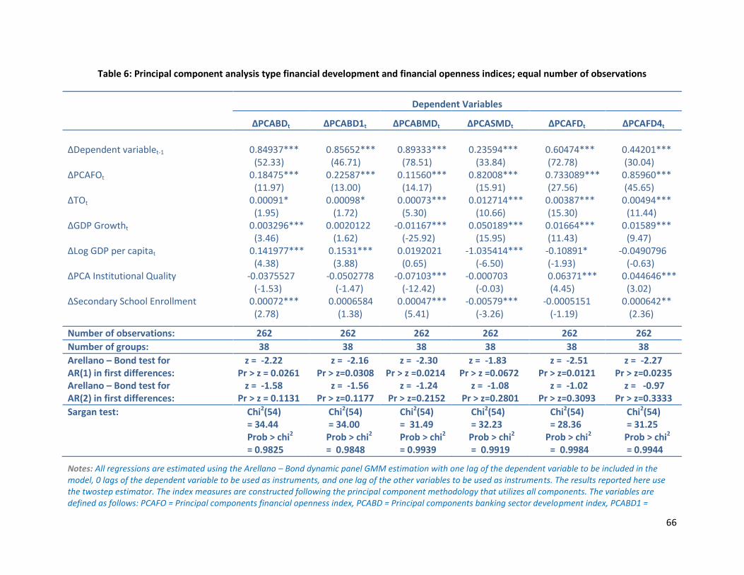
66
Table 6: Principal component analysis type financial development and financial openness indices; equal number of observations
Dependent Variables
∆PCABDt ∆PCABD1t ∆PCABMDt ∆PCASMDt ∆PCAFDt ∆PCAFD4t
∆Dependent variablet-1 0.84937*** (52.33)
0.85652*** (46.71)
0.89333*** (78.51)
0.23594*** (33.84)
0.60474*** (72.78)
0.44201*** (30.04)
∆PCAFOt 0.18475*** (11.97)
0.22587*** (13.00)
0.11560*** (14.17)
0.82008*** (15.91)
0.733089*** (27.56)
0.85960*** (45.65)
∆TOt 0.00091* (1.95)
0.00098* (1.72)
0.00073*** (5.30)
0.012714*** (10.66)
0.00387*** (15.30)
0.00494*** (11.44)
∆GDP Growtht 0.003296*** (3.46)
0.0020122 (1.62)
-0.01167*** (-25.92)
0.050189*** (15.95)
0.01664*** (11.43)
0.01589*** (9.47)
∆Log GDP per capitat 0.141977*** (4.38)
0.1531*** (3.88)
0.0192021 (0.65)
-1.035414*** (-6.50)
-0.10891* (-1.93)
-0.0490796 (-0.63)
∆PCA Institutional Quality -0.0375527 (-1.53)
-0.0502778 (-1.47)
-0.07103*** (-12.42)
-0.000703 (-0.03)
0.06371*** (4.45)
0.044646*** (3.02)
∆Secondary School Enrollment 0.00072*** (2.78)
0.0006584 (1.38)
0.00047*** (5.41)
-0.00579*** (-3.26)
-0.0005151 (-1.19)
0.000642** (2.36)
Number of observations: 262 262 262 262 262 262
Number of groups: 38 38 38 38 38 38
Arellano – Bond test for AR(1) in first differences: Arellano – Bond test for AR(2) in first differences:
z = -2.22 Pr > z = 0.0261 z = -1.58 Pr > z = 0.1131
z = -2.16 Pr > z=0.0308 z = -1.56 Pr > z=0.1177
z = -2.30 Pr > z =0.0214 z = -1.24 Pr > z=0.2152
z = -1.83 Pr > z =0.0672 z = -1.08 Pr > z=0.2801
z = -2.51 Pr > z=0.0121 z = -1.02 Pr > z=0.3093
z = -2.27 Pr > z=0.0235 z = -0.97 Pr > z=0.3333
Sargan test: Chi2(54) = 34.44 Prob > chi2 = 0.9825
Chi2(54) = 34.00 Prob > chi2 = 0.9848
Chi2(54) = 31.49 Prob > chi2
= 0.9939
Chi2(54) = 32.23 Prob > chi2 = 0.9919
Chi2(54) = 28.36 Prob > chi2 = 0.9984
Chi2(54) = 31.25 Prob > chi2 = 0.9944
Notes: All regressions are estimated using the Arellano – Bond dynamic panel GMM estimation with one lag of the dependent variable to be included in the model, 0 lags of the dependent variable to be used as instruments, and one lag of the other variables to be used as instruments. The results reported here use the twostep estimator. The index measures are constructed following the principal component methodology that utilizes all components. The variables are defined as follows: PCAFO = Principal components financial openness index, PCABD = Principal components banking sector development index, PCABD1 =

67
Principal components banking sector development index that excludes the deposit money banks to central bank assets ratio, PCABMD = Principal components bond market development index, PCASMD = Principal components stock market development index, PCAFD = Principal components financial development index, PCFD4 = Principal components financial development index that excludes the deposit money bank assets to central bank assets ratio. Institutional quality index is constructed using the principal components methodology. Figures in brackets are t-statistics and the stars represent the significant t-statistics for 1%, 5%, and 10% confidence levels respectively.
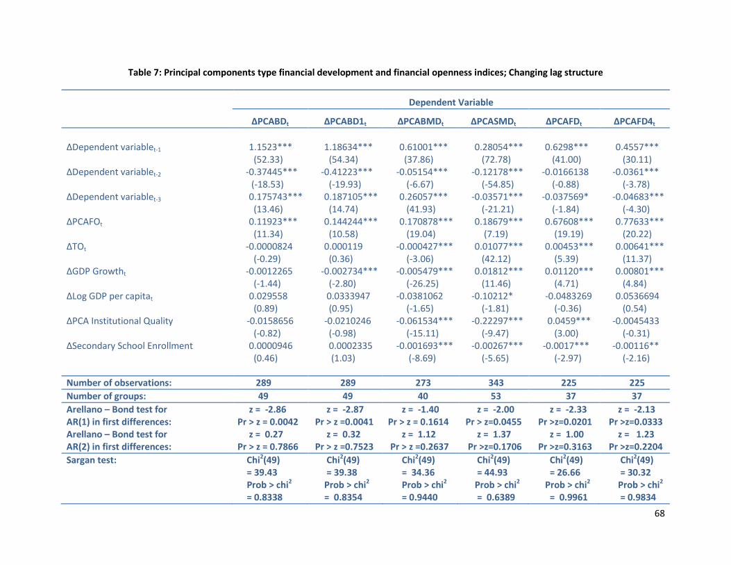
68
Table 7: Principal components type financial development and financial openness indices; Changing lag structure
Dependent Variable
∆PCABDt ∆PCABD1t ∆PCABMDt ∆PCASMDt ∆PCAFDt ∆PCAFD4t
∆Dependent variablet-1 1.1523*** (52.33)
1.18634*** (54.34)
0.61001*** (37.86)
0.28054*** (72.78)
0.6298*** (41.00)
0.4557*** (30.11)
∆Dependent variablet-2 -0.37445*** (-18.53)
-0.41223*** (-19.93)
-0.05154*** (-6.67)
-0.12178*** (-54.85)
-0.0166138 (-0.88)
-0.0361*** (-3.78)
∆Dependent variablet-3 0.175743*** (13.46)
0.187105*** (14.74)
0.26057*** (41.93)
-0.03571*** (-21.21)
-0.037569* (-1.84)
-0.04683*** (-4.30)
∆PCAFOt 0.11923*** (11.34)
0.144244*** (10.58)
0.170878*** (19.04)
0.18679*** (7.19)
0.67608*** (19.19)
0.77633*** (20.22)
∆TOt -0.0000824 (-0.29)
0.000119 (0.36)
-0.000427*** (-3.06)
0.01077*** (42.12)
0.00453*** (5.39)
0.00641*** (11.37)
∆GDP Growtht -0.0012265 (-1.44)
-0.002734*** (-2.80)
-0.005479*** (-26.25)
0.01812*** (11.46)
0.01120*** (4.71)
0.00801*** (4.84)
∆Log GDP per capitat 0.029558 (0.89)
0.0333947 (0.95)
-0.0381062 (-1.65)
-0.10212* (-1.81)
-0.0483269 (-0.36)
0.0536694 (0.54)
∆PCA Institutional Quality -0.0158656 (-0.82)
-0.0210246 (-0.98)
-0.061534*** (-15.11)
-0.22297*** (-9.47)
0.0459*** (3.00)
-0.0045433 (-0.31)
∆Secondary School Enrollment 0.0000946 (0.46)
0.0002335 (1.03)
-0.001693*** (-8.69)
-0.00267*** (-5.65)
-0.0017*** (-2.97)
-0.00116** (-2.16)
Number of observations: 289 289 273 343 225 225
Number of groups: 49 49 40 53 37 37
Arellano – Bond test for AR(1) in first differences: Arellano – Bond test for AR(2) in first differences:
z = -2.86 Pr > z = 0.0042 z = 0.27 Pr > z = 0.7866
z = -2.87 Pr > z =0.0041 z = 0.32 Pr > z =0.7523
z = -1.40 Pr > z = 0.1614 z = 1.12 Pr > z =0.2637
z = -2.00 Pr > z=0.0455 z = 1.37 Pr >z=0.1706
z = -2.33 Pr >z=0.0201 z = 1.00 Pr >z=0.3163
z = -2.13 Pr >z=0.0333 z = 1.23 Pr >z=0.2204
Sargan test: Chi2(49) = 39.43 Prob > chi2 = 0.8338
Chi2(49) = 39.38 Prob > chi2 = 0.8354
Chi2(49) = 34.36 Prob > chi2
= 0.9440
Chi2(49) = 44.93 Prob > chi2 = 0.6389
Chi2(49) = 26.66 Prob > chi2 = 0.9961
Chi2(49) = 30.32 Prob > chi2 = 0.9834
69
Notes: All regressions are estimated using the Arellano – Bond dynamic panel GMM estimation with 3 lags of the dependent variable to be included in the model, 0 lags of the dependent variable to be used as instruments, and 3 lags of the other variables to be used as instruments. The results reported here use the twostep estimator. The index measures are constructed following the principal component methodology that utilizes all components. The variables are defined as follows: PCAFO = Principal components financial openness index, PCABD = Principal components banking sector development index, PCABD1 = Principal components banking sector development index that excludes the deposit money banks to central bank assets ratio, PCABMD = Principal components bond market development index, PCASMD = Principal components stock market development index, PCAFD = Principal components financial development index, PCFD4 = Principal components financial development index that excludes the deposit money bank assets to central bank assets ratio. Institutional quality index is constructed using the principal components methodology. Figures in brackets are t-statistics and the stars represent the significant t-statistics for 1%, 5%, and 10% confidence levels respectively.
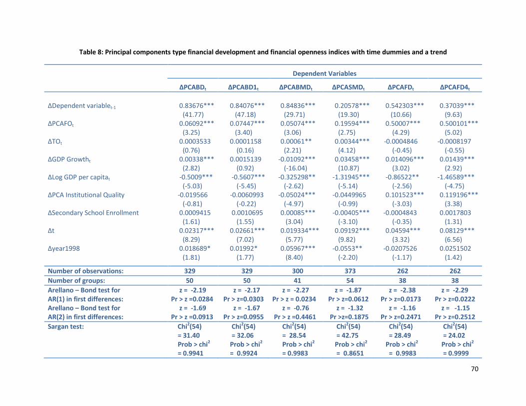
70
Table 8: Principal components type financial development and financial openness indices with time dummies and a trend
Dependent Variables
∆PCABDt ∆PCABD1t ∆PCABMDt ∆PCASMDt ∆PCAFDt ∆PCAFD4t
∆Dependent variablet-1 0.83676*** (41.77)
0.84076*** (47.18)
0.84836*** (29.71)
0.20578*** (19.30)
0.542303*** (10.66)
0.37039*** (9.63)
∆PCAFOt 0.06092*** (3.25)
0.07447*** (3.40)
0.05074*** (3.06)
0.19594*** (2.75)
0.50007*** (4.29)
0.500101*** (5.02)
∆TOt 0.0003533 (0.76)
0.0001158 (0.16)
0.00061** (2.21)
0.00344*** (4.12)
-0.0004846 (-0.45)
-0.0008197 (-0.55)
∆GDP Growtht 0.00338*** (2.82)
0.0015139 (0.92)
-0.01092*** (-16.04)
0.03458*** (10.87)
0.014096*** (3.02)
0.01439*** (2.92)
∆Log GDP per capitat -0.5009*** (-5.03)
-0.5607*** (-5.45)
-0.325298** (-2.62)
-1.31945*** (-5.14)
-0.86522** (-2.56)
-1.46589*** (-4.75)
∆PCA Institutional Quality -0.019566 (-0.81)
-0.0060993 (-0.22)
-0.05024*** (-4.97)
-0.0449965 (-0.99)
0.101523*** (-3.03)
0.119196*** (3.38)
∆Secondary School Enrollment 0.0009415 (1.61)
0.0010695 (1.55)
0.00085*** (3.04)
-0.00405*** (-3.10)
-0.0004843 (-0.35)
0.0017803 (1.31)
∆t 0.02317*** (8.29)
0.02661*** (7.02)
0.019334*** (5.77)
0.09192*** (9.82)
0.04594*** (3.32)
0.08129*** (6.56)
∆year1998 0.018689* (1.81)
0.01992* (1.77)
0.05967*** (8.40)
-0.0553** (-2.20)
-0.0207526 (-1.17)
0.0251502 (1.42)
Number of observations: 329 329 300 373 262 262
Number of groups: 50 50 41 54 38 38
Arellano – Bond test for AR(1) in first differences: Arellano – Bond test for AR(2) in first differences:
z = -2.19 Pr > z =0.0284 z = -1.69 Pr > z =0.0913
z = -2.17 Pr > z=0.0303 z = -1.67 Pr > z=0.0955
z = -2.27 Pr > z = 0.0234 z = -0.76 Pr > z =0.4461
z = -1.87 Pr > z=0.0612 z = -1.32 Pr >z=0.1875
z = -2.38 Pr > z=0.0173 z = -1.16 Pr > z=0.2471
z = -2.29 Pr > z=0.0222 z = -1.15 Pr > z=0.2512
Sargan test: Chi2(54) = 31.40 Prob > chi2 = 0.9941
Chi2(54) = 32.06 Prob > chi2 = 0.9924
Chi2(54) = 28.54 Prob > chi2
= 0.9983
Chi2(54) = 42.75 Prob > chi2 = 0.8651
Chi2(54) = 28.49 Prob > chi2 = 0.9983
Chi2(54) = 24.02 Prob > chi2 = 0.9999

71
Notes: All regressions are estimated using the Arellano – Bond dynamic panel GMM estimation with one lag of the dependent variable to be included in the
model, 0 lags of the dependent variable to be used as instruments, and one lag of the other variables to be used as instruments. The results reported here use
the twostep estimator. The index measures are constructed following the principal component methodology that utilizes all components. The variables are
defined as follows: PCAFO = Principal components financial openness index, PCABD = Principal components banking sector development index, PCABD1 =
Principal components banking sector development index that excludes the deposit money banks to central bank assets ratio, PCABMD = Principal components
bond market development index, PCASMD = Principal components stock market development index, PCAFD = Principal components financial development
index, PCFD4 = Principal components financial development index that excludes the deposit money bank assets to central bank assets ratio. Institutional quality
index is constructed using the principal components methodology. Figures in brackets are t-statistics and the stars represent the significant t-statistics for 1%,
5%, and 10% confidence levels respectively.

72
Table 9: Principal components type financial development and financial openness indices for the developing country sample
Dependent Variables
∆PCABDt ∆PCABD1t ∆PCABMDt ∆PCASMDt ∆PCAFDt ∆PCAFD4t
∆Dependent variablet-1 0.844134*** (37.54)
0.75831*** (24.67)
0.60517*** (13.54)
0.23144*** (43.53)
0.46032*** (8.45)
0.58921*** (3.38)
∆PCAFOt 0.05967*** (7.95)
0.06260*** (5.79)
0.02662*** (2.31)
0.38857*** (15.70)
0.08031*** (7.95)
0.13934*** (6.74)
∆TOt -0.00183*** (-5.00)
-0.001274* (-1.68)
-0.0008384 (-1.57)
0.00775*** (5.28)
0.0027243 (1.12)
0.0000593 (0.01)
∆GDP Growtht -0.00775*** (-3.74)
-0.0047189 (-1.40)
-0.00651*** (-6.61)
0.013346*** (10.98)
-0.00881*** (-6.27)
-0.007631* (-1.68)
∆Log GDP per capitat 0.39747*** (4.22)
0.3801*** (2.32)
-0.0886657 (-0.59)
-0.63521*** (-4.60)
0.277662 (1.31)
0.2301466 (0.31)
∆PCA Institutional Quality -0.04267** (-2.22)
-0.0203214 (-0.77)
-0.19296*** (-4.65)
-0.21788*** (-5.06)
-0.1873293 (-1.04)
-0.25922*** (-4.15)
∆Secondary School Enrollment -0.00358*** (-3.77)
-0.0015018 (-0.72)
0.00505*** (4.19)
-0.00367* (-1.93)
0.0015686 (0.58)
-0.00807** (-2.22)
Number of observations: 152 152 111 163 100 100
Number of groups: 25 25 18 27 16 16
Arellano – Bond test for AR(1) in first differences: Arellano – Bond test for AR(2) in first differences:
z = -1.76 Pr > z = 0.0778 z = 1.19 Pr > z = 0.2347
z = -1.93 Pr > z =0.0537 z = 0.99 Pr > z =0.3239
z = -1.69 Pr > z = 0.0920 z = 1.95 Pr > z =0.0510
z = -1.79 Pr > z =0.0741 z = -1.62 Pr > z=0.1049
z = -1.81 Pr > z=0.0701 z = -0.04 Pr > z=0.9680
z = -1.79 Pr > z=0.0729 z = -0.28 Pr > z=0.7760
Sargan test: Chi2(54) = 22.78 Prob > chi2 = 0.9999
Chi2(54) = 20.19 Prob > chi2 = 1.0000
Chi2(54) = 9.28 Prob > chi2
= 1.0000
Chi2(54) = 15.54 Prob > chi2 = 1.0000
Chi2(54) = 8.00 Prob > chi2 = 1.0000
Chi2(54) = 11.93 Prob > chi2 = 1.0000
Notes: All regressions are estimated using the Arellano – Bond dynamic panel GMM estimation with one lag of the dependent variable to be included in the model, 0 lags of the dependent variable to be used as instruments, and one lag of the other variables to be used as instruments. The results reported here use the twostep estimator. The index measures are constructed following the principal component methodology that utilizes all components. The variables are defined as follows: PCAFO = Principal components financial openness index, PCABD = Principal components banking sector development index, PCABD1 =

73
Principal components banking sector development index that excludes the deposit money banks to central bank assets ratio, PCABMD = Principal components bond market development index, PCASMD = Principal components stock market development index, PCAFD = Principal components financial development index, PCFD4 = Principal components financial development index that excludes the deposit money bank assets to central bank assets ratio. Institutional quality index is constructed using the principal components methodology. Figures in brackets are t-statistics and the stars represent the significant t-statistics for 1%, 5%, and 10% confidence levels respectively.

74
ADDITIONAL WEB APPENDICES
DATA APPENDIX
Financial openness indicators:
Market capitalization of listed companies (% of GDP): This variable represents the openness of the stock
market and the public consensus regarding the value of equities of companies as countries become more
globalized. It is equal to the value of listed shares divided by GDP. It is mostly used to represent a company’s
net worth and it is a decisive variable for stock valuation.69 Source: World Bank’s World Development
Indicators Database (2007)
Foreign direct investment: It is the sum of net inflows and outflows of foreign direct investment recorded as
a percentage of GDP. This indicator is brings together equity capital, reinvestment earning and other short
and long-term capital. It is one of the most frequently used indicators in the capital flows, financial
openness/globalization literature. Source: World Bank’s World Development Indicators Database (2007)
Number of domestic companies listed per million population: This variable is defined as the domestically
incorporated companies listed on the country’s stock exchanges at the end of the year.70 Domestic
companies listed do not include investment companies, mutual funds, or other collective investment
vehicles. As Baltagi, Demetriades and Law (2007) express, the number of domestic companies listed
provides a range of access to the capital market by new companies as financial liberalization takes place.71 It
is another measure for market size. Number of domestic companies listed and market capitalization of listed
companies both facilitate in observing the overall financial system as the barriers to entry of foreign firms
are being lifted. These two measures serve in understanding the stock market perspective of the openness
debate. Source: Beck, Demirguc-Kunt and Levine’s Database on Financial Development and Structure (2007)
Portfolio investment flows (% of GDP): These flows sum portfolio debt flows (public and publicly guaranteed
and private nonguaranteed bond issues purchased by foreign investors) and non-debt-creating portfolio
equity flows which are equal to the sum of country funds, depository receipts, and direct purchases of
shares by foreign investors.72 They exclude the liabilities constituting foreign authorities’ reserves. Portfolio
investment flows are used as an indicator for private capital flows. Portfolio flows are divided by the GDP in
current US dollars obtained from the World Bank’s World Development Indicators and are represented as a
percentage of GDP. Portfolio investment flows together with foreign direct investment represent the
incoming stream of investment and capital opportunities that the countries attract as a result of opening up
69
Huang, Wei, “Emerging Markets, Financial Openness, and Financial Development”, University of Bristol Discussion Paper, 2006 – 588, pp. 9 70
World Bank, 2007 World Development Indicators, International Bank for Reconstruction and Development/The World Bank Press, 2007, pp. 279 71
Baltagi, Badi, Panicos Demetriades, and Siong Hook Law, “Financial Development, Openness, and Institutions: Evidence from Panel Data”, Paper presented at the IMF Conference on New Perspectives on Financial Globalization, 2007, pp. 10 72
World Bank, 2007 World Development Indicators, International Bank for Reconstruction and Development/The World Bank Press, 2007, pp. 343

75
their financial markets. These types of flow variables are particularly useful in determining an efficient
financial openness measure. Source: World Bank’s World Development Indicators Database (2007)
International debt issues (% of GDP): International debt flows measures the net flow of international bond
issues relative to a country’s economic activity.73 This variable increases in the income level. Examining
country wide data we can observe that high-income countries are the group with the highest issues of
international debt relative to GDP. This indicator measures “the degree to which a country’s financial system
is interlinked with international financial markets”.74 This variable assists in examining the net flows of bond
issues and in bringing a view from the bond market. Source: Beck, Demirguc-Kunt and Levine’s Database on
Financial Development and Structure (2007)
Financial development indicators
a) Banking sector development indicators:
Liquid liabilities (% of GDP): It is the sum of currency, demand and interest bearing liabilities of banks and
other financial intermediaries divided by GDP represented as a percentage. Liquid liabilities is the broadest
indicator of financial intermediation due its inclusion of three financial sectors. 75 Source: Beck, Demirguc-
Kunt and Levine’s Database on Financial Development and Structure (2007)
Private credit by deposit money banks and other institutions (% of GDP): It is an indicator for the overall
development in private banking markets.76 This variable refers to financial resources provided to the private
sector by deposit money banks and other financial institutions through loans, purchases of nonequity
securities, and trade credits. Source: Beck, Demirguc-Kunt and Levine’s Database on Financial Development
and Structure (2007)
The ratio of deposit money bank assets to the sum of deposit money bank assets and central bank assets (in
percentages): It is equal to the deposit money bank assets divided by the sum of deposit money bank assets
and central bank assets. Source: Beck, Demirguc-Kunt and Levine’s Database on Financial Development and
Structure (2007)
Deposit money bank assets to central bank assets ratio (in percentages): It is measured as the ratio of
deposit money bank claims on domestic nonfinancial real sector to central bank claims on domestic
nonfinancial real sector. Source: Beck, Demirguc-Kunt and Levine’s Database on Financial Development and
Structure (2007)
Total bank assets (% of GDP): It is the sum of central bank assets to GDP and deposit money bank assets to
GDP. It is used to represent the overall size of the banking sector. Source: Beck, Demirguc-Kunt and Levine’s
Database on Financial Development and Structure (2007)
73
Beck, Thorsten, and Asli Demirguc-Kunt, “Financial Institutions and Markets Across Countries and Over Time – Data and Analysis”, World Bank Working Paper, (2009), pp. 15 74
Ibid., pp. 15 75
Ibid., pp. 22 76
Chinn, Menzie, and Hiro Ito, “What matters for financial development? Capital controls, institutions, and interactions”, Journal of Development Economics, (2006), pp. 5
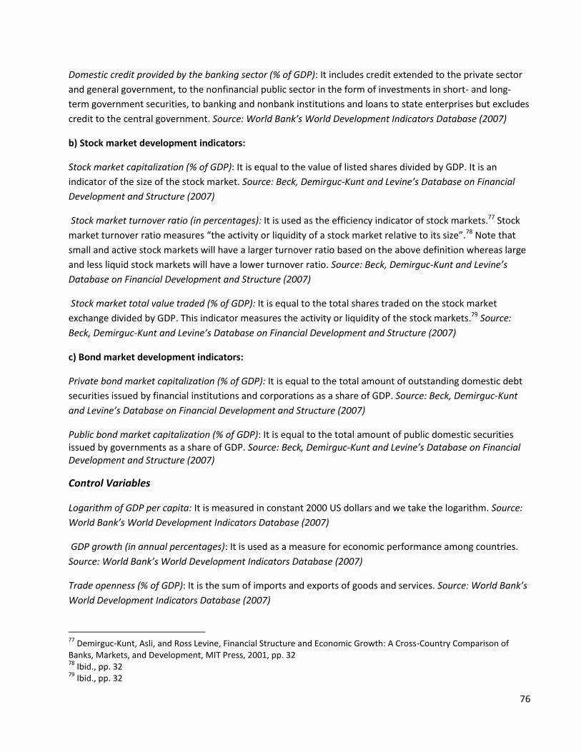
76
Domestic credit provided by the banking sector (% of GDP): It includes credit extended to the private sector
and general government, to the nonfinancial public sector in the form of investments in short- and long-
term government securities, to banking and nonbank institutions and loans to state enterprises but excludes
credit to the central government. Source: World Bank’s World Development Indicators Database (2007)
b) Stock market development indicators:
Stock market capitalization (% of GDP): It is equal to the value of listed shares divided by GDP. It is an
indicator of the size of the stock market. Source: Beck, Demirguc-Kunt and Levine’s Database on Financial
Development and Structure (2007)
Stock market turnover ratio (in percentages): It is used as the efficiency indicator of stock markets.77 Stock
market turnover ratio measures “the activity or liquidity of a stock market relative to its size”.78 Note that
small and active stock markets will have a larger turnover ratio based on the above definition whereas large
and less liquid stock markets will have a lower turnover ratio. Source: Beck, Demirguc-Kunt and Levine’s
Database on Financial Development and Structure (2007)
Stock market total value traded (% of GDP): It is equal to the total shares traded on the stock market
exchange divided by GDP. This indicator measures the activity or liquidity of the stock markets.79 Source:
Beck, Demirguc-Kunt and Levine’s Database on Financial Development and Structure (2007)
c) Bond market development indicators:
Private bond market capitalization (% of GDP): It is equal to the total amount of outstanding domestic debt
securities issued by financial institutions and corporations as a share of GDP. Source: Beck, Demirguc-Kunt
and Levine’s Database on Financial Development and Structure (2007)
Public bond market capitalization (% of GDP): It is equal to the total amount of public domestic securities issued by governments as a share of GDP. Source: Beck, Demirguc-Kunt and Levine’s Database on Financial Development and Structure (2007)
Control Variables
Logarithm of GDP per capita: It is measured in constant 2000 US dollars and we take the logarithm. Source:
World Bank’s World Development Indicators Database (2007)
GDP growth (in annual percentages): It is used as a measure for economic performance among countries.
Source: World Bank’s World Development Indicators Database (2007)
Trade openness (% of GDP): It is the sum of imports and exports of goods and services. Source: World Bank’s
World Development Indicators Database (2007)
77
Demirguc-Kunt, Asli, and Ross Levine, Financial Structure and Economic Growth: A Cross-Country Comparison of Banks, Markets, and Development, MIT Press, 2001, pp. 32 78
Ibid., pp. 32 79
Ibid., pp. 32

77
Secondary school gross enrolment rate (% of population): It is used as an indicator that controls for
differences in educational attainment across countries. We take secondary school gross enrollment rate as a
possible determinant for why we examine differences across countries in terms of grasping the benefits of
financial liberalization. Source: World Bank’s Edstats Database
Legal and institutional variable: They are used to measure the economic institutions and the overall quality
of legal systems. We employ four different measures to control for institutional, legal, political and
economic factors that may affect the overall level of financial development. The four variables used reflect
the “statistical compilation of responses on the quality of governance given by a large number of enterprise,
citizen and expert survey respondents in industrial and developing countries, as reported by a number of
survey institutes, think tanks, non-governmental organizations, and international organizations”.80 These
indicators are government effectiveness, regulatory quality, rule of law, and control corruption and are
measured through a range from-2.5 to 2.5 where higher values correspond to better governance outcomes.
Source: World Bank’s World Governance Indicators
80
World Governance Indicators (WGI) dataset, World Bank, http://info.worldbank.org/governance/wgi/index.asp

78
SUPPLEMENTARY APPENDIX
Table 1 (a): Summary of pairwise correlations for the financial openness variables and indices
Notes: Market capitalization: market capitalization of listed companies (% of GDP), FDI= Foreign direct investment (% of GDP), List of domestic companies =
number of domestic companies listed (per million population), international debt issues (% of GDP), portfolio investment = portfolio investment flows (% of
GDP), EFO = Equally weighted financial openness index, CFO = Coefficient of variation type financial openness index, PCFO = First score principal component type
financial openness index, PCAFO= Principal component type financial openness index. * represents the significances at the %5 percent level.
Variables Market cap.
FDI List of dom. Com.
Int. debt issues
Portfolio investment
EFO CFO PCFO PCAFO
Market Capitalization 1.0000 FDI 0.1961* 1.0000 List of domestic companies 0.5267* 0.2031* 1.0000 International debt issues 0.3212* 0.5409* 0.2204* 1.0000 Portfolio investment 0.0722 0.9224* 0.1053* 0.4588* 1.0000 EFO 0.7003* 0.7985* 0.5746* 0.6433* 0.6837* 1.0000 CFO 0.2525* 0.9812* 0.2548* 0.5622* 0.9620* 0.8361* 1.0000 PCFO 0.4457* 0.9149* 0.4186* 0.7399* 0.8514* 0.9428* 0.9471* 1.0000 PCAFO 0.6224* 0.7501* 0.7229* 0.6332* 0.6535* 0.9706* 0.7999* 0.9226* 1.0000
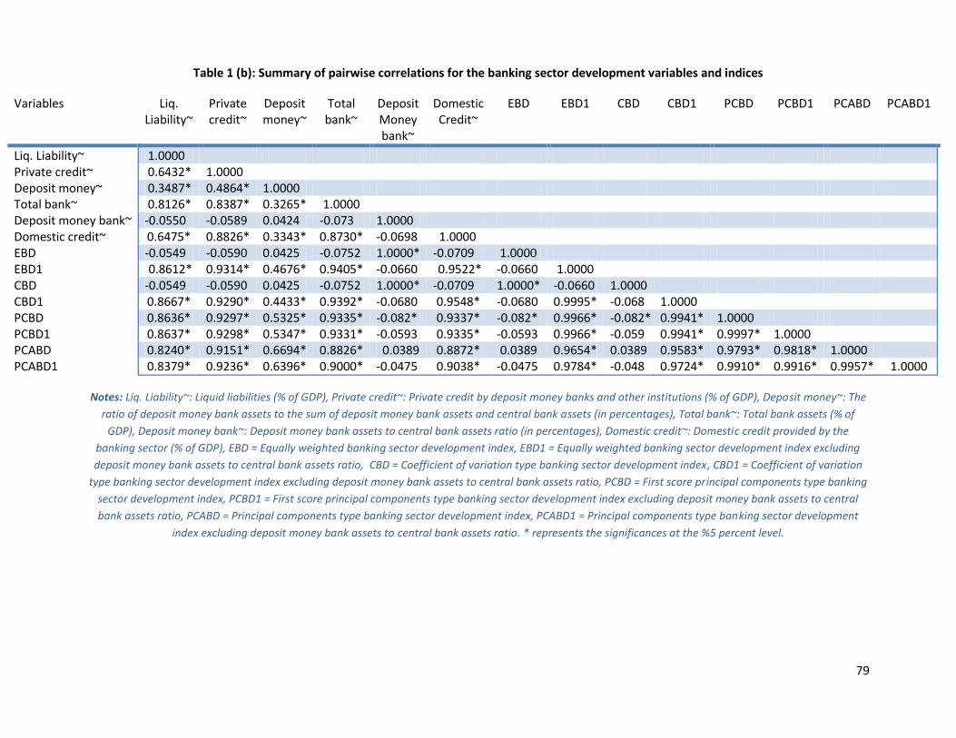
79
Table 1 (b): Summary of pairwise correlations for the banking sector development variables and indices
Variables Liq. Liability~
Private credit~
Deposit money~
Total bank~
Deposit Money bank~
Domestic Credit~
EBD EBD1 CBD CBD1 PCBD PCBD1 PCABD PCABD1
Liq. Liability~ 1.0000 Private credit~ 0.6432* 1.0000 Deposit money~ 0.3487* 0.4864* 1.0000 Total bank~ 0.8126* 0.8387* 0.3265* 1.0000 Deposit money bank~ -0.0550 -0.0589 0.0424 -0.073 1.0000 Domestic credit~ 0.6475* 0.8826* 0.3343* 0.8730* -0.0698 1.0000 EBD -0.0549 -0.0590 0.0425 -0.0752 1.0000* -0.0709 1.0000 EBD1 0.8612* 0.9314* 0.4676* 0.9405* -0.0660 0.9522* -0.0660 1.0000 CBD -0.0549 -0.0590 0.0425 -0.0752 1.0000* -0.0709 1.0000* -0.0660 1.0000 CBD1 0.8667* 0.9290* 0.4433* 0.9392* -0.0680 0.9548* -0.0680 0.9995* -0.068 1.0000 PCBD 0.8636* 0.9297* 0.5325* 0.9335* -0.082* 0.9337* -0.082* 0.9966* -0.082* 0.9941* 1.0000 PCBD1 0.8637* 0.9298* 0.5347* 0.9331* -0.0593 0.9335* -0.0593 0.9966* -0.059 0.9941* 0.9997* 1.0000 PCABD 0.8240* 0.9151* 0.6694* 0.8826* 0.0389 0.8872* 0.0389 0.9654* 0.0389 0.9583* 0.9793* 0.9818* 1.0000 PCABD1 0.8379* 0.9236* 0.6396* 0.9000* -0.0475 0.9038* -0.0475 0.9784* -0.048 0.9724* 0.9910* 0.9916* 0.9957* 1.0000
Notes: Liq. Liability~: Liquid liabilities (% of GDP), Private credit~: Private credit by deposit money banks and other institutions (% of GDP), Deposit money~: The
ratio of deposit money bank assets to the sum of deposit money bank assets and central bank assets (in percentages), Total bank~: Total bank assets (% of
GDP), Deposit money bank~: Deposit money bank assets to central bank assets ratio (in percentages), Domestic credit~: Domestic credit provided by the
banking sector (% of GDP), EBD = Equally weighted banking sector development index, EBD1 = Equally weighted banking sector development index excluding
deposit money bank assets to central bank assets ratio, CBD = Coefficient of variation type banking sector development index, CBD1 = Coefficient of variation
type banking sector development index excluding deposit money bank assets to central bank assets ratio, PCBD = First score principal components type banking
sector development index, PCBD1 = First score principal components type banking sector development index excluding deposit money bank assets to central
bank assets ratio, PCABD = Principal components type banking sector development index, PCABD1 = Principal components type banking sector development
index excluding deposit money bank assets to central bank assets ratio. * represents the significances at the %5 percent level.

80
Table 1 (c): Summary of pairwise correlations for the bond market development variables and indices
Variables Private bond~
Public bond~ EBMD CBMD PCBMD PCABMD
Private bond market capitalization 1.0000 Public bond market capitalization 0.3451* 1.0000 EBMD 0.8456* 0.7928* 1.0000 CBMD 0.9232* 0.6794* 0.9858* 1.0000 PCBMD 0.8201* 0.8201* 0.9989* 0.9770* 1.0000 PCABMD 0.9606* 0.5924* 0.9607* 0.9936* 0.9469* 1.0000
Notes: Private bond~:Private bond market capitalization (% of GDP), Public bond~: Public bond market capitalization (% of GDP), EBMD = Equally weighted
bond market development index, CBMD = Coefficient of variation type bond market development index, PCBMD = First score principal components type bond
market development index, PCABMD = Principal components type bond market development index. * represents the significances at the %5 percent level.
Table 1 (d): Summary of pairwise correlations for the stock market development variables and indices
Variables Stock market caitalization
Stock market turnover
Stock market total value
traded
ESMD CSMD PCSMD PCASMD
Stock market capitalization 1.0000 Stock market turnover 0.1084* 1.0000 Stock market total value traded 0.6862* 0.6003* 1.0000 ESMD 0.7443* 0.7120* 0.9498* 1.0000 CSMD 0.7156* 0.7279* 0.9593* 0.9987* 1.0000 PCSMD 0.7591* 0.6822* 0.9620* 0.9987* 0.9978* 1.0000 PCASMD 0.5480* 0.8635* 0.9104* 0.9656* 0.9735* 0.9561* 1.0000
Notes: Stock market capitalization: Stock market capitalization (% of GDP), Stock market turnover ratio (in percentages), Stock market total value traded (% of
GDP), ESMD = Equally weighted bond market development index, ESMD = Equally weighted stock market development index, CSMD = Coefficient of variation
type stock market development index, PCSMD = First score principal components type stock market development index, PCASMD = Principal components type
stock market development index. * represents the significances at the %5 percent level.

81
Table 2: Principal component type financial development and financial openness indices adjusted by their means
Dependent Variables
∆MEPCABDt ∆MEPCABD1t ∆MEPCABMDt ∆MEPCASMDt ∆MEPCAFDt ∆MEPCAFD4t
∆Mean adjusted dependent variablet-1 0.76194*** (67.47)
0.77124*** (135.2)
0.91726*** (137.9)
0.3343*** (142.3)
0.42044*** (68.12)
0.39434*** (44.87)
∆MEPCAFOt -0.00494*** (-7.668)
-0.00657*** (-5.760)
-0.00150*** (-3.466)
0.0107*** (6.819)
0.05291*** (26.13)
0.06108*** (20.90)
∆TOt 0.00172*** (12.50)
0.00199*** (13.80)
0.00198*** (15.42)
0.0130*** (67.62)
0.0117*** (21.13)
0.0126*** (20.92)
∆GDP Growtht -0.00370*** (-13.09)
-0.00444*** (-9.464)
-0.0119*** (-52.07)
0.0430*** (43.46)
0.0144*** (7.533)
0.0170*** (7.357)
∆Log GDP per capitat 0.20176*** (13.70)
0.23933*** (14.20)
0.0430*** (2.650)
0.5721*** (17.55)
0.33211*** (5.552)
0.44315*** (7.264)
∆MEPCA Institutional Quality -0.02367*** (-21.86)
-0.02541*** (-15.73)
-0.0666*** (-39.10)
-0.224*** (-26.38)
-0.0881*** (-5.516)
-0.1234*** (-8.988)
∆Secondary School Enrollment -0.000650*** (-3.762)
-0.0009*** (-3.881)
-0.000829*** (-12.56)
-0.00547*** (-15.01)
-0.00331*** (-14.95)
-0.00314*** (-9.030)
Number of observations: 329 329 300 373 262 262
Number of groups: 50 50 41 54 38 38
Arellano – Bond test for AR(1) in first differences: Arellano – Bond test for AR(2) in first differences:
z = -1.36 Pr > z = 0.1737 z = -1.30 Pr > z = 0.1919
z = -1.40 Pr > z=0.1624 z = -1.29 Pr > z=0.1979
z = -2.39 Pr > z =0.0167 z = -1.55 Pr > z=0.1219
z = -2.09 Pr > z =0.0370 z = -0.89 Pr > z=0.3742
z = -2.21 Pr >z=0.0268 z = -0.86 Pr >z=0.3871
z = -2.23 Pr >z=0.0260 z = -0.80 Pr >z=0.4243
Sargan test: Chi2(54) = 45.71 Prob > chi2 = 0.7815
Chi2(54) = 44.52 Prob > chi2 = 0.8178
Chi2(54) = 37.22 Prob > chi2
= 0.9603
Chi2(54) = 49.01 Prob > chi2 = 0.6669
Chi2(54) = 31.07 Prob > chi2 = 0.9984
Chi2(54) = 30.74 Prob > chi2 = 0.9955
Notes: All regressions are estimated using the Arellano – Bond dynamic panel GMM estimation with one lag of the dependent variable to be included in the model, 0 lags of the dependent variable to be used as instruments, and one lag of the other variables to be used as instruments. The results reported here use
the twostep estimator. All index measures are mean adjusted. These index measures are constructed following the principal component methodology that utilizes all components. The variables are defined as follows: MEPCAFO =Mean adjusted principal components financial openness index, MEPCABD = Mean
adjusted principal components banking sector development index, MEPCABD1 = Mean adjusted principal components banking sector development index that

82
excludes the deposit money banks to central bank assets ratio, MEPCABMD = Mean adjusted principal components bond market development index, MEPCASMD = Mean adjusted principal components stock market development index, MEPCAFD = Mean adjusted principal components financial development index, MEPCFD4 = Mean adjusted principal components financial development index that excludes the deposit money bank assets to central bank assets ratio. Institutional quality index is constructed using the principal components methodology. MEPCA Institutional quality= Mean adjusted principal component type
institutional quality index. Figures in brackets are t-statistics and the stars represent t-statistics for 1%, 5%, and %10 confidence levels.

83
Table 3: Principal component type financial development and financial openness indices, excluding control variables of institutional quality
index and secondary school enrollment rate
∆PCABDt ∆PCABD1t ∆PCABMDt ∆PCASMDt ∆PCAFDt ∆PCAFD4t
Models (a) (b) (a) (b) (a) (b) (a) (b) (a) (b) (a) (b)
∆Dependent
variablet-1
.8646***
(103.33)
.87120***
(204.77)
.86717***
(118.23)
.87304***
(179.23)
.8632***
(117.84)
.8292***
(62.00)
.3103***
(180.44)
.25195***
(119.63)
.5962***
(58.30)
.58840***
(89.11)
.46342***
(69.81)
.43659***
(30.84)
∆PCAFOt .1754***
(24.99)
.02923***
(3.08)
.21763***
(30.10)
.04433***
(2.63)
.1497***
(16.41)
.0785***
(7.09)
.2298***
(11.89)
.19711***
(11.97)
.7063***
(23.31)
.42352***
(41.93)
.84526***
(51.16)
.54748***
(22.31)
∆TOt .0008***
(3.43)
-.0000977
(-0.47)
.00098***
(4.02)
.0002797
(1.27)
.0005***
(2.74)
.0005***
(3.16)
.0080***
(38.32)
.0002215
(1.08)
.0037***
(9.12)
.00201***
(12.60)
.00507***
(17.77)
.00194***
(4.97)
∆GDP Growtht .0013***
(2.91)
-.00129**
(-1.90)
.0001143
(0.26)
-.0023***
(-3.43)
-.0114***
(-45.15)
-.010***
(-34.44)
.0330***
(40.62)
.03340***
(45.12)
.0137***
(-7.52)
.0121909
(8.00)
.01729***
(16.99)
.00716***
(3.25)
∆Log GDP per
capitat
.0692***
(2.59)
.3563***
(13.10)
.0818***
(2.73)
.38187***
(10.38)
-.02965**
(-1.48)
.06491**
(2.27)
.10383**
(1.71)
1.078***
(26.27)
.0225963
(0.32)
.4431226
(6.77)
-.0939***
(-2.60)
.64371***
(8.83)
∆PCAInstitutio-
nal Quality
- -.02005**
(-1.68)
- -.0449***
(-5.24)
- -.082***
(-24.67)
- -.1699***
(-15.52)
- .0235216
(1.54)
- .0091028
(0.64)
∆Secondary
School
Enrollment
.0010***
(5.30)
- .00110***
(5.07)
- -.00037**
(-2.15)
- -.004***
(-8.98)
- -.0013***
(-3.28)
- .00055**
(2.15)
-
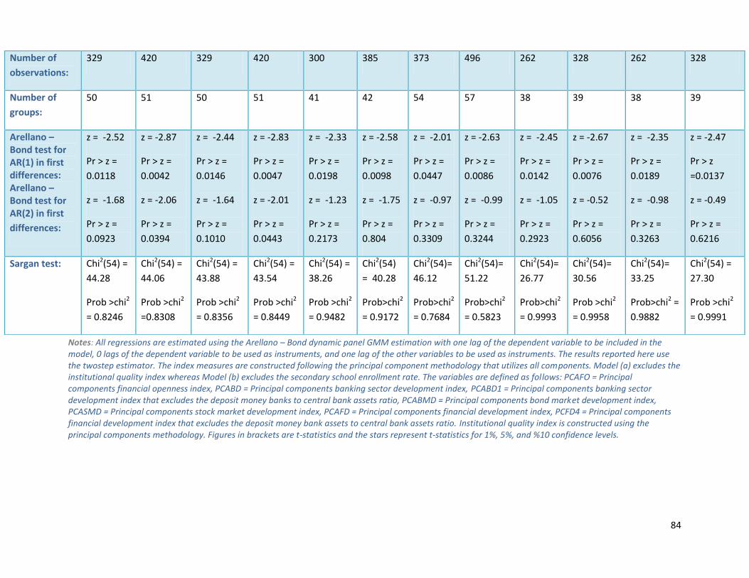
84
Notes: All regressions are estimated using the Arellano – Bond dynamic panel GMM estimation with one lag of the dependent variable to be included in the model, 0 lags of the dependent variable to be used as instruments, and one lag of the other variables to be used as instruments. The results reported here use the twostep estimator. The index measures are constructed following the principal component methodology that utilizes all components. Model (a) excludes the institutional quality index whereas Model (b) excludes the secondary school enrollment rate. The variables are defined as follows: PCAFO = Principal components financial openness index, PCABD = Principal components banking sector development index, PCABD1 = Principal components banking sector development index that excludes the deposit money banks to central bank assets ratio, PCABMD = Principal components bond market development index, PCASMD = Principal components stock market development index, PCAFD = Principal components financial development index, PCFD4 = Principal components financial development index that excludes the deposit money bank assets to central bank assets ratio. Institutional quality index is constructed using the principal components methodology. Figures in brackets are t-statistics and the stars represent t-statistics for 1%, 5%, and %10 confidence levels.
Number of
observations:
329 420 329 420 300 385 373 496 262 328 262 328
Number of
groups:
50 51 50 51 41 42 54 57 38 39 38 39
Arellano – Bond test for AR(1) in first differences: Arellano – Bond test for AR(2) in first
differences:
z = -2.52
Pr > z =
0.0118
z = -1.68
Pr > z =
0.0923
z = -2.87
Pr > z =
0.0042
z = -2.06
Pr > z =
0.0394
z = -2.44
Pr > z =
0.0146
z = -1.64
Pr > z =
0.1010
z = -2.83
Pr > z =
0.0047
z = -2.01
Pr > z =
0.0443
z = -2.33
Pr > z =
0.0198
z = -1.23
Pr > z =
0.2173
z = -2.58
Pr > z =
0.0098
z = -1.75
Pr > z =
0.804
z = -2.01
Pr > z =
0.0447
z = -0.97
Pr > z =
0.3309
z = -2.63
Pr > z =
0.0086
z = -0.99
Pr > z =
0.3244
z = -2.45
Pr > z =
0.0142
z = -1.05
Pr > z =
0.2923
z = -2.67
Pr > z =
0.0076
z = -0.52
Pr > z =
0.6056
z = -2.35
Pr > z =
0.0189
z = -0.98
Pr > z =
0.3263
z = -2.47
Pr > z
=0.0137
z = -0.49
Pr > z =
0.6216
Sargan test: Chi2(54) =
44.28
Prob >chi2
= 0.8246
Chi2(54) =
44.06
Prob >chi2
=0.8308
Chi2(54) =
43.88
Prob >chi2
= 0.8356
Chi2(54) =
43.54
Prob >chi2
= 0.8449
Chi2(54) =
38.26
Prob >chi2
= 0.9482
Chi2(54)
= 40.28
Prob>chi2
= 0.9172
Chi2(54)=
46.12
Prob>chi2
= 0.7684
Chi2(54)=
51.22
Prob>chi2
= 0.5823
Chi2(54)=
26.77
Prob>chi2
= 0.9993
Chi2(54)=
30.56
Prob >chi2
= 0.9958
Chi2(54)=
33.25
Prob>chi2 =
0.9882
Chi2(54) =
27.30
Prob >chi2
= 0.9991
85
Table 4: Principal component type financial development and financial openness indices, predetermined variables
Dependent Variables
∆PCABDt ∆PCABD1t ∆PCABMDt ∆PCASMDt ∆PCAFDt ∆PCAFD4t
∆Dependent variablet-1 0.85356*** (98.27)
0.85302*** (117.36)
0.83843*** (33.69)
0.30953*** (44.25)
0.66462*** (25.46)
0.50773*** (25.54)
∆PCAFOt 0.20042*** (8.95)
0.27345*** (11.00)
0.10854*** (7.23)
0.16656*** (4.91)
0.85077*** (41.51)
1.08361*** (28.70)
∆TOt -0.000513 (-1.26)
-0.00116*** (-2.82)
-0.00098*** (-4.32)
0.01166*** (23.56)
0.00310*** (7.07)
0.00384*** (7.16)
∆GDP Growtht -0.000572 (-0.83)
-0.00162** (-2.13)
-0.00756*** (-21.13)
0.02164*** (6.52)
0.01519*** (6.89)
0.01262*** (5.58)
∆Log GDP per capitat 0.15938*** (6.03)
0.18541*** (6.00)
0.13306*** (5.56)
0.18515** (1.90)
-0.10165 (-1.26)
-0.10732** (-1.73)
∆PCA Institutional Quality -0.07817*** (-2.40)
-0.05497** (-1.90)
-0.081705*** (-39.10)
-0.37460*** (-19.68)
0.10857** (1.83)
0.07534** (1.79)
∆Secondary School Enrollment 0.00063* (1.29)
0.00012*** (0.23)
-0.001066*** (-4.02)
-0.014225*** (-20.18)
-0.000829 (-1.12)
-0.00056 (-0.84)
Number of observations: 329 329 300 373 262 262
Number of groups: 50 50 41 54 38 38
Arellano – Bond test for AR(1) in first differences: Arellano – Bond test for AR(2) in first differences:
z = -2.49 Pr > z = 0.0129 z = -1.80 Pr > z = 0.0716
z = -2.43 Pr > z =0.0149 z = -1.73 Pr > z =0.0840
z = -2.26 Pr > z =0.0240 z = -1.34 Pr > z=0.1739
z = -1.92 Pr > z =0.0553 z = -1.01 Pr > z=0.3113
z = -2.54 Pr >z=0.0110 z = -1.04 Pr >z=0.2987
z = -2.32 Pr >z=0.0201 z = -1.05 Pr >z=0.2937
Sargan test: Chi2(108) = 41.34 Prob > chi2 = 1.0000
Chi2(108) = 44.40 Prob > chi2 = 1.0000
Chi2(108) = 39.58 Prob > chi2
= 1.0000
Chi2(108) = 49.55 Prob > chi2 = 1.0000
Chi2(108) = 34.13 Prob > chi2 = 1.0000
Chi2(108) = 33.10 Prob > chi2 = 1.0000
Notes: All regressions are estimated using the Arellano – Bond dynamic panel GMM estimation with one lag of the dependent variable to be included in the model, 0 lags of the dependent variable to be used as instruments, and one lag of the other variables to be used as instruments. The results reported here use the twostep estimator. The index measures are constructed following the principal component methodology that utilizes all components. All variables with the
exception of the lag of the dependent variable are treated as being predetermined. The variables are defined as follows: PCAFO = Principal components financial openness index, PCABD = Principal components banking sector development index, PCABD1 = Principal components banking sector development index that

86
excludes the deposit money banks to central bank assets ratio, PCABMD = Principal components bond market development index, PCASMD = Principal components stock market development index, PCAFD = Principal components financial development index, PCFD4 = Principal components financial development
index that excludes the deposit money bank assets to central bank assets ratio. Institutional quality index is constructed using the principal components methodology. Figures in brackets are t-statistics and the stars represent t-statistics for 1%, 5%, and %10 confidence levels.
87
Table 5: Principal component type financial development and financial openness indices, endogenous variables
Dependent Variables
∆PCABDt ∆PCABD1t ∆PCABMDt ∆PCASMDt ∆PCAFDt ∆PCAFD4t
∆Dependent variablet-1 0.8753*** (81.67)
0.8738*** (79.90)
0.84279*** (39.11)
0.29763*** (47.18)
0.61170*** (36.48)
0.4478*** (18.85)
∆PCAFOt 0.22080*** (10.49)
0.2804*** (11.53)
0.08947*** (5.97)
0.19891*** (5.20)
0.94161*** (25.04)
1.1869*** (24.26)
∆TOt -0.00265*** (-5.67)
-0.00296*** (-5.84)
-0.00054** (-1.95)
0.01140*** (21.97)
0.001502** (1.84)
0.00276*** (2.44)
∆GDP Growtht 0.00174*** (3.28)
0.00081* (1.29)
-0.00990*** (-21.49)
0.03574*** (12.22)
0.01662*** (8.09)
0.01751*** (21.80)
∆Log GDP per capitat 0.22506*** (10.85)
0.24787*** (9.92)
0.14803*** (5.41)
-0.136158 (-1.08)
-0.10941 (-1.01)
-0.146371* (-1.56)
∆PCA Institutional Quality 0.01308 (0.65)
0.00368 (0.17)
-0.09542*** (-8.61)
-0.39572*** (-15.19)
0.06084 (1.18)
-0.004402 (-0.12)
∆Secondary School Enrollment -0.00167** (-2.22)
-0.00189** (-2.03)
-0.000773** (-1.78)
-0.01631*** (-9.23)
-0.00239** (-2.10)
0.00124 (1.10)
Number of observations: 329 329 300 373 262 262
Number of groups: 50 50 41 54 38 38
Arellano – Bond test for AR(1) in first differences: Arellano – Bond test for AR(2) in first differences:
z = -2.74 Pr > z = 0.0062 z = -1.78 Pr > z = 0.0744
z = -2.65 Pr > z =0.0080 z = -1.74 Pr > z =0.0827
z = -2.35 Pr > z =0.0187 z = -1.29 Pr > z=0.1972
z = -1.94 Pr > z =0.0526 z = -1.09 Pr > z
=0.2762
z = -2.49 Pr >z=0.0129 z = -1.17 Pr >z=0.2406
z = -2.26 Pr >z=0.0241 z = -1.17 Pr >z=0.2439
Sargan test: Chi2(108) = 43.76 Prob > chi2 = 1.0000
Chi2(108) = 43.66 Prob > chi2 = 1.0000
Chi2(108) = 38.26 Prob > chi2
= 1.0000
Chi2(108) = 50.35 Prob > chi2 = 1.0000
Chi2(108) = 34.37 Prob > chi2 = 1.0000
Chi2(108) = 34.99 Prob > chi2 = 1.0000
Notes: All regressions are estimated using the Arellano – Bond dynamic panel GMM estimation with one lag of the dependent variable to be included in the model, 0 lags of the dependent variable to be used as instruments, and one lag of the other variables to be used as instruments. The results reported here use the twostep estimator. The index measures are constructed following the principal component methodology that utilizes all components. All variables with the exception of the lag of the dependent variable are treated as being endogenous. The variables are defined as follows: PCAFO = Principal components financial

88
openness index, PCABD = Principal components banking sector development index, PCABD1 = Principal components banking sector development index that excludes the deposit money banks to central bank assets ratio, PCABMD = Principal components bond market development index, PCASMD = Principal
components stock market development index, PCAFD = Principal components financial development index, PCFD4 = Principal components financial development index that excludes the deposit money bank assets to central bank assets ratio. Institutional quality index is constructed using the principal components
methodology. Figures in brackets are t-statistics and the stars represent t-statistics for 1%, 5%, and %10 confidence levels.
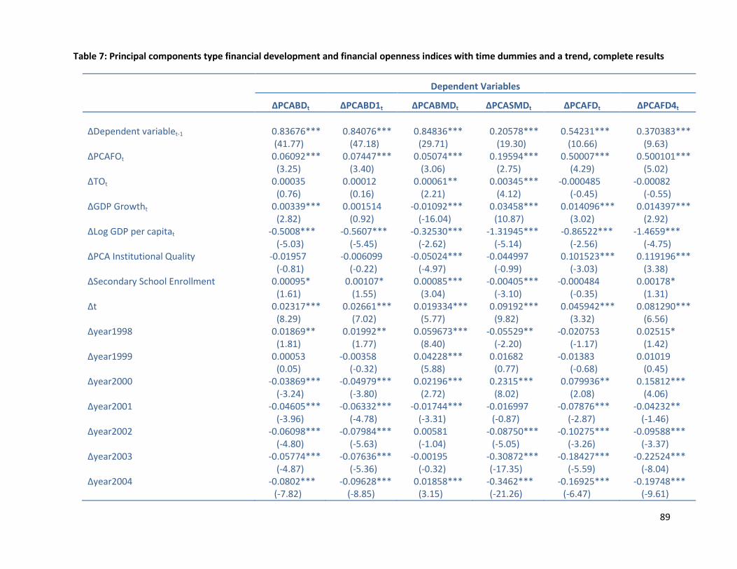
89
Table 7: Principal components type financial development and financial openness indices with time dummies and a trend, complete results
Dependent Variables
∆PCABDt ∆PCABD1t ∆PCABMDt ∆PCASMDt ∆PCAFDt ∆PCAFD4t
∆Dependent variablet-1 0.83676*** (41.77)
0.84076*** (47.18)
0.84836*** (29.71)
0.20578*** (19.30)
0.54231*** (10.66)
0.370383*** (9.63)
∆PCAFOt 0.06092*** (3.25)
0.07447*** (3.40)
0.05074*** (3.06)
0.19594*** (2.75)
0.50007*** (4.29)
0.500101*** (5.02)
∆TOt 0.00035 (0.76)
0.00012 (0.16)
0.00061** (2.21)
0.00345*** (4.12)
-0.000485 (-0.45)
-0.00082 (-0.55)
∆GDP Growtht 0.00339*** (2.82)
0.001514 (0.92)
-0.01092*** (-16.04)
0.03458*** (10.87)
0.014096*** (3.02)
0.014397*** (2.92)
∆Log GDP per capitat -0.5008*** (-5.03)
-0.5607*** (-5.45)
-0.32530*** (-2.62)
-1.31945*** (-5.14)
-0.86522*** (-2.56)
-1.4659*** (-4.75)
∆PCA Institutional Quality -0.01957 (-0.81)
-0.006099 (-0.22)
-0.05024*** (-4.97)
-0.044997 (-0.99)
0.101523*** (-3.03)
0.119196*** (3.38)
∆Secondary School Enrollment 0.00095* (1.61)
0.00107* (1.55)
0.00085*** (3.04)
-0.00405*** (-3.10)
-0.000484 (-0.35)
0.00178* (1.31)
∆t 0.02317*** (8.29)
0.02661*** (7.02)
0.019334*** (5.77)
0.09192*** (9.82)
0.045942*** (3.32)
0.081290*** (6.56)
∆year1998 0.01869** (1.81)
0.01992** (1.77)
0.059673*** (8.40)
-0.05529** (-2.20)
-0.020753 (-1.17)
0.02515* (1.42)
∆year1999 0.00053 -0.00358 0.04228*** 0.01682 -0.01383 0.01019 (0.05) (-0.32) (5.88) (0.77) (-0.68) (0.45) ∆year2000 -0.03869*** -0.04979*** 0.02196*** 0.2315*** 0.079936** 0.15812*** (-3.24) (-3.80) (2.72) (8.02) (2.08) (4.06) ∆year2001 -0.04605*** -0.06332*** -0.01744*** -0.016997 -0.07876*** -0.04232** (-3.96) (-4.78) (-3.31) (-0.87) (-2.87) (-1.46) ∆year2002 -0.06098*** -0.07984*** 0.00581 -0.08750*** -0.10275*** -0.09588*** (-4.80) (-5.63) (-1.04) (-5.05) (-3.26) (-3.37) ∆year2003 -0.05774*** -0.07636*** -0.00195 -0.30872*** -0.18427*** -0.22524*** (-4.87) (-5.36) (-0.32) (-17.35) (-5.59) (-8.04) ∆year2004 -0.0802*** -0.09628*** 0.01858*** -0.3462*** -0.16925*** -0.19748*** (-7.82) (-8.85) (3.15) (-21.26) (-6.47) (-9.61)

90
∆year2005 -0.04020*** -0.04678*** -0.03087*** -0.26550*** -0.11033*** -0.145713*** (-4.83) (-5.77) (-4.25) (-18.18) (-5.76) (-7.75) ∆year2006 -0.03723*** -0.04563*** -0.0257*** -0.25209*** -0.09977*** -0.11913*** (-6.22)
(-6.55) (-3.59) (-17.51) (-5.69) (-8.69)
Number of observations: 329 329 300 373 262 262
Number of groups: 50 50 41 54 38 38
Arellano – Bond test for AR(1) in first differences: Arellano – Bond test for AR(2) in first differences:
z = -2.19 Pr > z =0.0284 z = -1.69 Pr > z =0.0913
z = -2.17 Pr > z=0.0303 z = -1.67 Pr > z=0.0955
z = -2.27 Pr > z = 0.0234 z = -0.76 Pr > z =0.4461
z = -1.87 Pr > z =0.0612 z = -1.32 Pr > z=0.1875
z = -2.38 Pr > z=0.0173 z = -1.16 Pr > z=0.2471
z = -2.29 Pr > z=0.0222 z = -1.15 Pr > z=0.2512
Sargan test: Chi2(54) = 31.40 Prob > chi2 = 0.9941
Chi2(54) = 32.06 Prob > chi2 = 0.9924
Chi2(54) = 28.54 Prob > chi2
= 0.9983
Chi2(54) = 42.75 Prob > chi2 = 0.8651
Chi2(54) = 28.49 Prob > chi2 = 0.9983
Chi2(54) = 24.02 Prob > chi2 = 0.9999
Notes: All regressions are estimated using the Arellano – Bond dynamic panel GMM estimation with one lag of the dependent variable to be included in the
model, 0 lags of the dependent variable to be used as instruments, and one lag of the other variables to be used as instruments. The results reported here use
the twostep estimator. The index measures are constructed following the principal component methodology that utilizes all components. The model above
includes a linear time trend and time dummies. The variables are defined as follows: PCAFO = Principal components financial openness index, PCABD = Principal
components banking sector development index, PCABD1 = Principal components banking sector development index that excludes the deposit money banks to
central bank assets ratio, PCABMD = Principal components bond market development index, PCASMD = Principal components stock market development index,
PCAFD = Principal components financial development index, PCFD4 = Principal components financial development index that excludes the deposit money bank
assets to central bank assets ratio. Institutional quality index is constructed using the principal components methodology. Figures in brackets are t-statistics and
the stars represent t-statistics for 1%, 5%, and %10 confidence levels.

91
Table 8: Principal components type financial development and financial openness indices with time dummies
Dependent Variables
∆PCABDt ∆PCABD1t ∆PCABMDt ∆PCASMDt ∆PCAFDt ∆PCAFD4t
∆Dependent variablet-1 0.84355*** (34.10)
0.83795*** (41.39)
0.8301*** (24.96)
0.20455*** (14.72)
0.58265*** (11.25)
0.4327927*** (10.14)
∆PCAFOt 0.06913*** (3.76)
0.07702*** (3.40)
0.05142*** (3.16)
0.18548*** (3.27)
0.46010*** (7.61)
0.5292751*** (5.65)
∆TOt -0.00002 (-0.03)
0.00029 (0.50)
0.00086** (3.00)
0.00355*** (7.27)
-0.00007 (-0.06)
0.0001039 (0.06)
∆GDP Growtht 0.00308*** (3.60)
0.00218** (1.66)
-0.01145*** (-20.58)
0.03567*** (7.67)
0.01384*** (3.03)
0.0133873*** (2.74)
∆Log GDP per capitat -0.50117*** (-4.97)
-0.55298*** (-5.19)
-0.175442*** (-2.57)
-1.54424*** (-3.57)
-0.89022*** (-2.82)
-1.541898*** (-4.01)
∆PCA Institutional Quality 0.00936 (0.33)
0.00089 (0.04)
-0.05432*** (-5.34)
-0.04045 (-0.86)
0.07048** (2.06)
0.1185935*** (3.08)
∆Secondary School Enrollment 0.00143*** (2.63)
0.00173*** (2.55)
0.00095*** (2.86)
-0.004243*** (-3.43)
0.00005 (0.04)
0.0021574* (1.51)
∆year1998 0.04342*** (4.35)
0.05636*** (4.88)
0.06710*** (7.15)
0.027654 (1.13)
0.043610** (1.85)
0.118667* (4.40)
∆year1999 0.05849*** 0.05676*** 0.05962*** 0.20274*** 0.08914*** 0.1793196 (5.26) (3.67) (6.73) (5.81) (2.92) (4.52) ∆year2000 0.03964*** 0.03173* 0.05660*** 0.52527*** 0.236972*** 0.3919676*** (2.58) (1.47) (6.47) (8.86) (3.55) (5.60) ∆year2001 0.06601*** 0.04323** 0.02940*** 0.38038*** 0.12899** 0.2927506** (3.56) (1.72) (2.47) (5.55) (2.12) (4.07) ∆year2002 0.07551*** 0.05667** 0.06186*** 0.40316*** 0.154927*** 0.3287523*** (3.74) (1.96) (5.16) (5.45) (2.53) (4.54) ∆year2003 0.10026*** 0.08451*** 0.07904*** 0.28146*** 0.138351** 0.2983793*** (4.33) (2.72) (6.04) (3.49) (2.07) (3.65) ∆year2004 0.1014*** 0.08759*** 0.11577*** 0.34050*** 0.20772*** 0.4086914*** (3.97) (2.40) (8.40) (3.59) (2.43) (4.22) ∆year2005 0.16715*** 0.162413*** 0.07756*** 0.52375*** 0.30428*** 0.5295226*** (5.86) (3.88) (4.56) (4.74) (3.26) (4.94)
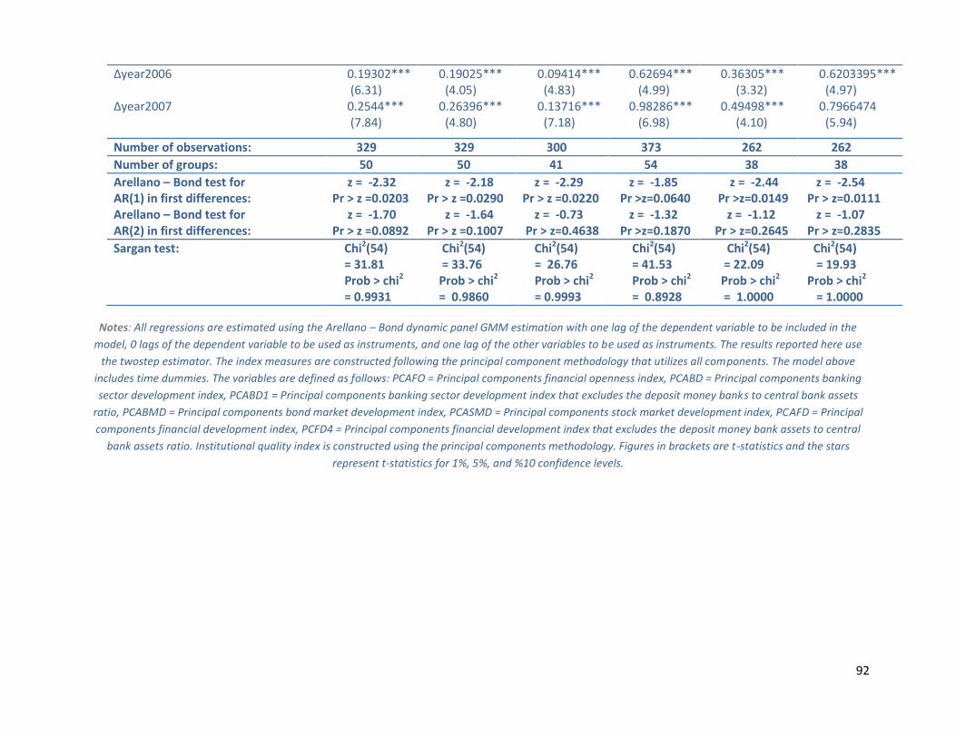
92
∆year2006 0.19302*** 0.19025*** 0.09414*** 0.62694*** 0.36305*** 0.6203395*** (6.31) (4.05) (4.83) (4.99) (3.32) (4.97) ∆year2007 0.2544***
(7.84)
0.26396*** (4.80)
0.13716*** (7.18)
0.98286*** (6.98)
0.49498*** (4.10)
0.7966474 (5.94)
Number of observations: 329 329 300 373 262 262
Number of groups: 50 50 41 54 38 38
Arellano – Bond test for AR(1) in first differences: Arellano – Bond test for AR(2) in first differences:
z = -2.32 Pr > z =0.0203 z = -1.70 Pr > z =0.0892
z = -2.18 Pr > z =0.0290 z = -1.64 Pr > z =0.1007
z = -2.29 Pr > z =0.0220 z = -0.73 Pr > z=0.4638
z = -1.85 Pr >z=0.0640 z = -1.32 Pr >z=0.1870
z = -2.44 Pr >z=0.0149 z = -1.12 Pr > z=0.2645
z = -2.54 Pr > z=0.0111 z = -1.07 Pr > z=0.2835
Sargan test: Chi2(54) = 31.81 Prob > chi2 = 0.9931
Chi2(54) = 33.76 Prob > chi2 = 0.9860
Chi2(54) = 26.76 Prob > chi2 = 0.9993
Chi2(54) = 41.53 Prob > chi2 = 0.8928
Chi2(54) = 22.09 Prob > chi2 = 1.0000
Chi2(54) = 19.93 Prob > chi2 = 1.0000
Notes: All regressions are estimated using the Arellano – Bond dynamic panel GMM estimation with one lag of the dependent variable to be included in the
model, 0 lags of the dependent variable to be used as instruments, and one lag of the other variables to be used as instruments. The results reported here use
the twostep estimator. The index measures are constructed following the principal component methodology that utilizes all components. The model above
includes time dummies. The variables are defined as follows: PCAFO = Principal components financial openness index, PCABD = Principal components banking
sector development index, PCABD1 = Principal components banking sector development index that excludes the deposit money banks to central bank assets
ratio, PCABMD = Principal components bond market development index, PCASMD = Principal components stock market development index, PCAFD = Principal
components financial development index, PCFD4 = Principal components financial development index that excludes the deposit money bank assets to central
bank assets ratio. Institutional quality index is constructed using the principal components methodology. Figures in brackets are t-statistics and the stars
represent t-statistics for 1%, 5%, and %10 confidence levels.

93
Table 9: Principal components type financial development and financial openness indices with time dummies and a trend
Dependent Variables
∆PCABDt ∆PCABD1t ∆PCABMDt ∆PCASMDt ∆PCAFDt ∆PCAFD4t
∆Dependent variablet-1 1.1304*** (39.42)
1.16364*** (39.68)
0.53056*** (12.86)
0.21979*** (25.98)
0.68672*** (11.42)
0.48552*** (12.45)
∆Dependent variablet-2 -0.3912*** -0.39947*** -0.02324 -0.15466*** -0.022323 -0.05661*** (-11.70) (-12.98) (-1.07) (-35.16) (-0.75) (-2.58) ∆Dependent variablet-3 0.17724*** 0.17827*** 0.24188*** -0.000901 0.04210 0.08282** (9.86) (10.89) (11.95) (-0.15) (1.05) (2.26) ∆PCAFOt 0.03264*
(1.46) 0.07336***
(2.25) 0.09571***
(6.51) 0.08576***
(1.76) 0.40269***
(7.06) 0.41688***
(6.37) ∆TOt -0.00054
(-0.89) -0.000062
(-0.07) 0.00008
(0.29) 0.00565***
(8.66) 0.00227 (1.22)
0.00236 (1.27)
∆GDP Growtht 0.000734 (0.45)
-0.000657 (-0.36)
-0.00613*** (-6.95)
0.02261*** (8.53)
0.00089 (0.22)
0.00496 (1.09)
∆Log GDP per capitat -0.590112*** (-4.16)
-0.58476*** (-2.79)
-0.316264*** (-4.71)
-2.48431*** (-9.12)
-0.8957** (-2.16)
-1.8038*** (-3.88)
∆PCA Institutional Quality 0.06757*** (2.52)
0.09809*** (2.76)
-0.036513*** (-4.94)
-0.090751*** (-3.52)
0.10820** (2.31)
0.12416*** (2.74)
∆Secondary School Enrollment 0.000763* (1.27)
0.00082* (1.30)
-0.000793*** (-2.47)
-0.00284** (-2.30)
-0.00020 (-0.12)
0.00107 (0.64)
∆t 0.02638*** (5.42)
0.0272*** (3.66)
0.01420*** (6.28)
0.12764*** (11.85)
0.03793*** (2.90)
0.07253*** (4.33)
∆year2000 -0.056317*** -0.06269*** -0.009492** 0.214588*** 0.12310*** 0.13789*** (-4.38) (-3.68) (-2.29) (11.38) (5.29) (4.13) ∆year2001 -0.043154*** -0.040735*** -0.036021*** -0.071995*** -0.11285*** -0.09596*** (-4.07) (-3.00) (-7.02) (-4.63) (-2.87) (-4.47) ∆year2002 -0.054824*** -0.042994** -0.02323*** -0.11637*** -0.10517*** -0.09558*** (-3.64) (-2.33) (-3.74) (-8.84) (-3.06) (-2.83) ∆year2003 -0.063674*** -0.06433*** -0.01583** -0.3560*** -0.166744*** -0.21296*** (-4.80) (-3.89) (-2.21) (-29.12) (-4.88) (-4.79) ∆year2004 -0.08588*** -0.08723*** 0.0087* -0.37503*** -0.123284*** -0.15444*** (-9.18) (-7.19) (1.35) (-31.23) (-4.56) (-4.24)

94
∆year2005 -0.027871*** -0.02496** -0.02421*** -0.32904*** -0.08308*** -0.118708*** (-2.95) (-2.28) (-3.38) (-24.48) (-3.86) (-4.12) ∆year2006 -0.04543*** -0.05348*** -0.02485*** -0.288475*** -0.07656*** -0.09518*** (-8.48)
(-8.23) (-4.28) (-19.86) (-4.80) (-4.47)
Number of observations: 289 289 273 343 225 225
Number of groups: 49 49 40 53 37 37
Arellano – Bond test for AR(1) in first differences: Arellano – Bond test for AR(2) in first differences:
z = -2.96 Pr > z = 0.0031 z = 0.12 Pr > z = 0.9058
z = -2.79 Pr > z=0.0053 z = -0.12 Pr > z =0.9067
z = -0.80 Pr > z = 0.4262 z = 1.97 Pr > z =0.0487
z = -2.02 Pr > z =0.0437 z = 1.32 Pr > z =0.1870
z = -2.91 Pr > z=0.0036 z = 2.61 Pr > z=0.0090
z = -2.74 Pr > z=0.0062 z = 2.65 Pr > z=0.0080
Sargan test: Chi2(49) = 26.95 Prob > chi2 = 0.9956
Chi2(49) = 26.96 Prob > chi2 = 0.9956
Chi2(49) = 24.36 Prob > chi2
= 0.9988
Chi2(49) = 43.10 Prob > chi2 = 0.7101
Chi2(49) = 17.77 Prob > chi2 = 1.0000
Chi2(49) = 17.73 Prob > chi2 = 1.0000
Notes: All regressions are estimated using the Arellano – Bond dynamic panel GMM estimation with three lags of the dependent variable to be included in the
model, 0 lags of the dependent variable to be used as instruments, and three lags of the other variables to be used as instruments. The results reported here use
the twostep estimator. The index measures are constructed following the principal component methodology that utilizes all components. The model above
includes a higher lag structure, a linear time trend and time dummies. The variables are defined as follows: PCAFO = Principal components financial openness
index, PCABD = Principal components banking sector development index, PCABD1 = Principal components banking sector development index that excludes the
deposit money banks to central bank assets ratio, PCABMD = Principal components bond market development index, PCASMD = Principal components stock
market development index, PCAFD = Principal components financial development index, PCFD4 = Principal components financial development index that
excludes the deposit money bank assets to central bank assets ratio. Institutional quality index is constructed using the principal components methodology.
Figures in brackets are t-statistics and the stars represent t-statistics for 1%, 5%, and %10 confidence levels.
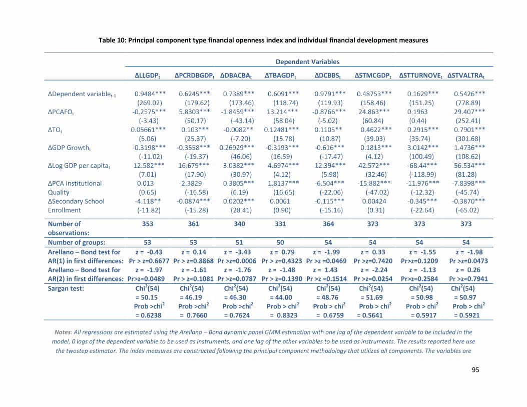
95
Table 10: Principal component type financial openness index and individual financial development measures
Dependent Variables
∆LLGDPt ∆PCRDBGDPt ∆DBACBAt ∆TBAGDPt ∆DCBBSt ∆STMCGDPt ∆STTURNOVEt ∆STVALTRAt
∆Dependent variablet-1 0.9484*** (269.02)
0.6245*** (179.62)
0.7389*** (173.46)
0.6091*** (118.74)
0.9791*** (119.93)
0.48753*** (158.46)
0.1629*** (151.25)
0.5426*** (778.89)
∆PCAFOt -0.2575*** (-3.43)
5.8303*** (50.17)
-1.8459*** (-43.14)
13.214*** (58.04)
-0.8766*** (-5.02)
24.863*** (60.84)
0.1963 (0.44)
29.407*** (252.41)
∆TOt 0.05661*** (5.06)
0.103*** (25.37)
-0.0082** (-7.20)
0.12481*** (15.78)
0.1105** (10.87)
0.4622*** (39.03)
0.2915*** (35.74)
0.7901*** (301.68)
∆GDP Growtht -0.3198*** (-11.02)
-0.3558*** (-19.37)
0.26929*** (46.06)
-0.3193*** (16.59)
-0.616*** (-17.47)
0.1813*** (4.12)
3.0142*** (100.49)
1.4736*** (108.62)
∆Log GDP per capitat 12.582*** (7.01)
16.679*** (17.90)
3.0382*** (30.97)
4.6974*** (4.12)
12.394*** (5.98)
42.572*** (32.46)
-68.44*** (-118.99)
56.534*** (81.28)
∆PCA Institutional Quality
0.013 (0.65)
-2.3829 (-16.58)
0.3805*** (6.19)
1.8137*** (16.65)
-6.504*** (-22.06)
-15.882*** (-47.02)
-11.976*** (-12.32)
-7.8398*** (-45.74)
∆Secondary School Enrollment
-4.118** (-11.82)
-0.0874*** (-15.28)
0.0202*** (28.41)
0.0061 (0.90)
-0.115*** (-15.16)
0.00424 (0.31)
-0.345*** (-22.64)
-0.3870*** (-65.02)
Number of observations:
353 361 340 331 364 373 373 373
Number of groups: 53 53 51 50 54 54 54 54
Arellano – Bond test for AR(1) in first differences: Arellano – Bond test for AR(2) in first differences:
z = -0.43 Pr > z=0.6677 z = -1.97
Pr>z=0.0489
z = 0.14 Pr > z=0.8868 z = -1.61 Pr > z=0.1081
z = -3.43 Pr >z=0.0006 z = -1.76 Pr >z=0.0787
z = 0.79 Pr > z=0.4323 z = -1.48 Pr > z=0.1390
z = -1.99 Pr >z =0.0469
z = 1.43 Pr >z =0.1514
z = 0.33 Pr >z=0.7420
z = -2.24 Pr >z=0.0254
z = -1.55 Pr>z=0.1209 z = -1.13 Pr>z=0.2584
z = -1.98 Pr >z=0.0473 z = 0.26
Pr >z=0.7941
Sargan test: Chi2(54) = 50.15 Prob >chi2 = 0.6238
Chi2(54) = 46.19 Prob >chi2 = 0.7660
Chi2(54) = 46.30 Prob >chi2
= 0.7624
Chi2(54) = 44.00 Prob > chi2 = 0.8323
Chi2(54) = 48.76 Prob > chi2 = 0.6759
Chi2(54) = 51.69 Prob > chi2 = 0.5641
Chi2(54) = 50.98 Prob > chi2 = 0.5917
Chi2(54) = 50.97 Prob > chi2
= 0.5921
Notes: All regressions are estimated using the Arellano – Bond dynamic panel GMM estimation with one lag of the dependent variable to be included in the
model, 0 lags of the dependent variable to be used as instruments, and one lag of the other variables to be used as instruments. The results reported here use
the twostep estimator. The index measures are constructed following the principal component methodology that utilizes all components. The variables are

96
defined as follows: LLGDP = Liquid liabilities (%of GDP), PCRDBOFGDP = Private credit by deposit money banks and other institutions (% of GDP), DBACBA = The
ratio of deposit money bank assets to the sum of deposit money bank assets to central bank assets (in percentages), TBAGDP = Total bank assets (% of GDP),
DCBBS = Domestic credit provided by the banking sector (% of GDP), STMCGDP = Stock market capitalization (% of GDP), STTURNOVER = Stock market turnover
ratio (in percentages), STVALTRA = Stock market total value traded (% of GDP), PCAFO = Principal components financial openness index. Institutional quality
index is constructed using the principal components methodology. Figures in brackets are t statistics and the stars represent the significant t-statistics for 1%,
5%, and % 10 confidence levels.
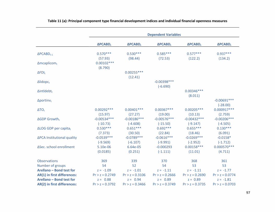
97
Table 11 (a): Principal component type financial development indices and individual financial openness measures
Dependent Variables
∆PCABDt ∆PCABDt ∆PCABDt ∆PCABDt ∆PCABDt
∆PCABDt-1 0.570*** 0.530*** 0.585*** 0.577*** 0.937*** (57.93) (98.44) (72.53) (122.2) (134.2) ∆mcaplicomt 0.00102*** (8.790) ∆FDIt 0.00255*** (12.41) ∆lidopct -0.00398*** (-6.690) ∆intldebtt 0.00346*** (8.011) ∆portinvt -0.00691*** (-28.00) ∆TOt 0.00292*** 0.00401*** 0.00367*** 0.00205*** 0.000917*** (15.97) (27.27) (19.00) (10.13) (2.759) ∆GDP Growtht -0.00534*** -0.00186*** -0.00576*** -0.00432*** -0.00206*** (-10.73) (-4.608) (-15.50) (-9.147) (-4.505) ∆LOG GDP per capitat 0.530*** 0.651*** 0.692*** 0.655*** 0.130*** (7.373) (30.50) (22.84) (18.46) (6.091) ∆PCA Institutional quality -0.0539*** -0.0789*** -0.0616*** -0.0269*** -0.0158* (-9.569) (-6.107) (-9.991) (-2.952) (-1.712) ∆Sec. school enrollment 5.10e-06 6.64e-05 -0.000293 0.00158*** 0.000570*** (0.0185) (0.251) (-1.111) (11.01) (4.711) Observations 369 339 370 368 361 Number of groups 54 52 54 53 53 Arellano – Bond test for AR(1) in first differences: Arellano – Bond test for AR(2) in first differences:
z = -1.09 Pr > z = 0.2749
z = 0.88 Pr > z = 0.3792
z = -1.01 Pr > z = 0.3106
z = 0.94 Pr > z = 0.3466
z = -1.11 Pr > z = 0.2666
z = 0.89 Pr > z = 0.3749
z = -1.11 Pr > z = 0.2690
z = 0.89 Pr > z = 0.3735
z = -1.77 Pr > z = 0.0774
z = -1.81 Pr > z = 0.0703
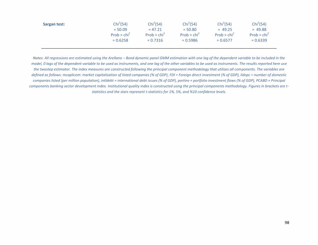
98
Sargan test: Chi2(54) = 50.09
Chi2(54) = 47.21
Chi2(54) = 50.80
Chi2(54) = 49.25
Chi2(54) = 49.88
Prob > chi2 = 0.6258
Prob > chi2 = 0.7316
Prob > chi2 = 0.5986
Prob > chi2 = 0.6577
Prob > chi2 = 0.6339
Notes: All regressions are estimated using the Arellano – Bond dynamic panel GMM estimation with one lag of the dependent variable to be included in the
model, 0 lags of the dependent variable to be used as instruments, and one lag of the other variables to be used as instruments. The results reported here use
the twostep estimator. The index measures are constructed following the principal component methodology that utilizes all components. The variables are
defined as follows: mcaplicom: market capitalization of listed companies (% of GDP), FDI = Foreign direct investment (% of GDP), lidopc = number of domestic
companies listed (per million population), intldebt = international debt issues (% of GDP), portinv = portfolio investment flows (% of GDP), PCABD = Principal
components banking sector development index. Institutional quality index is constructed using the principal components methodology. Figures in brackets are t-
statistics and the stars represent t-statistics for 1%, 5%, and %10 confidence levels.

99
Table 11 (b): Principal component type financial development indices and individual financial openness measures
Dependent Variables
∆PCABD1t ∆PCABD1t ∆PCABD1t ∆PCABD1t ∆PCABD1t
∆PCABD1t-1 0.684*** 0.606*** 0.692*** 0.663*** 0.966*** (83.94) (105.4) (87.85) (92.03) (75.07) ∆mcaplicomt 0.00130*** (11.07) ∆FDIt 0.00338*** (12.52) ∆lidopct -0.00300*** (-7.590) ∆intldebtt 0.00466*** (13.04) ∆portinvt -0.00603*** (-15.27) ∆TOt 0.00244*** 0.00425*** 0.00374*** 0.00169*** 0.000831** (11.07) (21.54) (14.37) (6.102) (2.192) ∆GDP Growtht -0.00701*** -0.00335*** -0.00733*** -0.00585*** -0.00426*** (-11.41) (-6.373) (-10.50) (-9.677) (-9.134) ∆Log of GDP per capitat 0.252*** 0.608*** 0.484*** 0.488*** 0.0875*** (4.050) (20.95) (13.17) (9.370) (3.268) ∆PCA Institutional quality -0.0487*** -0.0782*** -0.0517*** -0.00489 -0.0186** (-5.048) (-4.628) (-6.043) (-0.466) (-2.332) ∆Sec. school enrollment -0.000766*** -0.000253 -0.00106*** 0.00118*** 0.000230 (-2.682) (-0.788) (-4.768) (6.148) (1.481) Observations 369 339 370 368 361 Number of groups 54 52 54 53 53 Arellano – Bond test for AR(1) in first differences:
z = -1.05 Pr > z = 0.2934
z = -1.04 Pr > z = 0.2988
z = -1.06 Pr > z = 0.2903
z = -1.05 Pr > z = 0.2954
z = -2.79 Pr > z = 0.0052
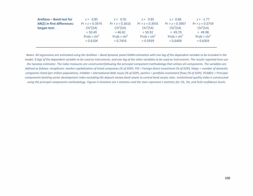
100
Arellano – Bond test for AR(2) in first differences:
z = 0.85 Pr > z = 0.3974
z = 0.91 Pr > z = 0.3616
z = 0.85 Pr > z = 0.3935
z = 0.86 Pr > z = 0.3907
z = -1.77 Pr > z = 0.0759
Sargan test: Chi2(54) = 50.49
Chi2(54) = 46.81
Chi2(54) = 50.92
Chi2(54) = 49.70
Chi2(54) = 49.98
Prob > chi2 = 0.6104
Prob > chi2 = 0.7454
Prob > chi2 = 0.5939
Prob > chi2 = 0.6409
Prob > chi2 = 0.6303
Notes: All regressions are estimated using the Arellano – Bond dynamic panel GMM estimation with one lag of the dependent variable to be included in the
model, 0 lags of the dependent variable to be used as instruments, and one lag of the other variables to be used as instruments. The results reported here use
the twostep estimator. The index measures are constructed following the principal component methodology that utilizes all components. The variables are
defined as follows: mcaplicom: market capitalization of listed companies (% of GDP), FDI = Foreign direct investment (% of GDP), lidopc = number of domestic
companies listed (per million population), intldebt = international debt issues (% of GDP), portinv = portfolio investment flows (% of GDP), PCABD1 = Principal
components banking sector development index excluding the deposit money bank assets to central bank assets ratio. Institutional quality index is constructed
using the principal components methodology. Figures in brackets are t-statistics and the stars represent t-statistics for 1%, 5%, and %10 confidence levels.
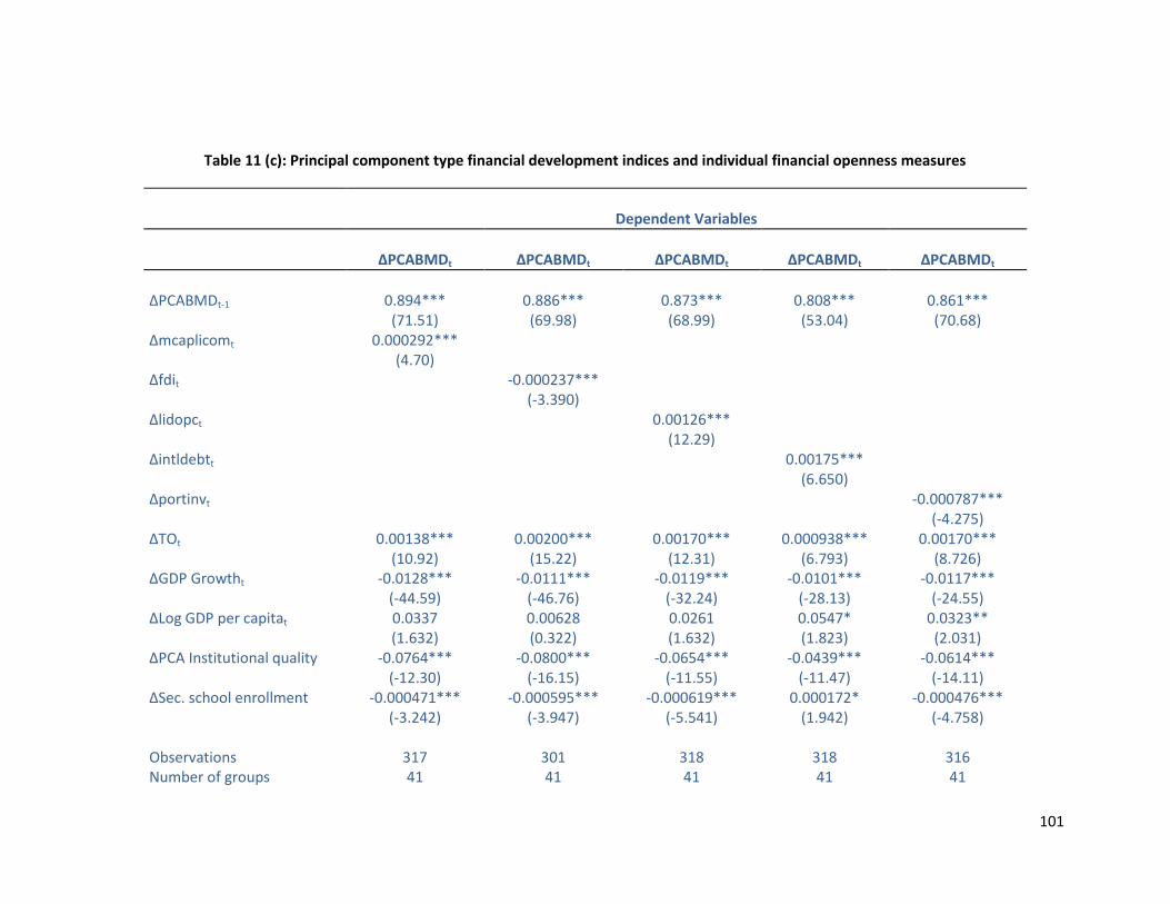
101
Table 11 (c): Principal component type financial development indices and individual financial openness measures
Dependent Variables
∆PCABMDt ∆PCABMDt ∆PCABMDt ∆PCABMDt ∆PCABMDt
∆PCABMDt-1 0.894*** 0.886*** 0.873*** 0.808*** 0.861*** (71.51) (69.98) (68.99) (53.04) (70.68) ∆mcaplicomt 0.000292*** (4.70) ∆fdit -0.000237*** (-3.390) ∆lidopct 0.00126*** (12.29) ∆intldebtt 0.00175*** (6.650) ∆portinvt -0.000787*** (-4.275) ∆TOt 0.00138*** 0.00200*** 0.00170*** 0.000938*** 0.00170*** (10.92) (15.22) (12.31) (6.793) (8.726) ∆GDP Growtht -0.0128*** -0.0111*** -0.0119*** -0.0101*** -0.0117*** (-44.59) (-46.76) (-32.24) (-28.13) (-24.55) ∆Log GDP per capitat 0.0337 0.00628 0.0261 0.0547* 0.0323** (1.632) (0.322) (1.632) (1.823) (2.031) ∆PCA Institutional quality -0.0764*** -0.0800*** -0.0654*** -0.0439*** -0.0614*** (-12.30) (-16.15) (-11.55) (-11.47) (-14.11) ∆Sec. school enrollment -0.000471*** -0.000595*** -0.000619*** 0.000172* -0.000476*** (-3.242) (-3.947) (-5.541) (1.942) (-4.758) Observations 317 301 318 318 316 Number of groups 41 41 41 41 41

102
Arellano – Bond test for AR(1) in first differences: Arellano – Bond test for AR(2) in first differences:
z = -2.48 Pr > z = 0.0131
z = -1.66 Pr > z = 0.0962
z = -2.54 Pr > z = 0.0109
z = -1.41 Pr > z = 0.1598
z = -2.58 Pr > z = 0.0098
z = -1.68 Pr > z = 0.0932
z = -2.43 Pr > z = 0.0152
z = -1.66 Pr > z = 0.0974
z = -2.52 Pr > z = 0.0119
z = -1.62 Pr > z = 0.1047
Sargan test: Chi2(54) = 35.11
Chi2(54) = 34.29
Chi2(54) = 34.38
Chi2(54) = 35.51
Chi2(54) = 33.25
Prob > chi2 = 0.9783
Prob > chi2 = 0.9833
Prob > chi2 = 0.9828
Prob > chi2 = 0.9756
Prob > chi2 = 0.9882
Notes: All regressions are estimated using the Arellano – Bond dynamic panel GMM estimation with one lag of the dependent variable to be included in the
model, 0 lags of the dependent variable to be used as instruments, and one lag of the other variables to be used as instruments. The results reported here use
the twostep estimator. The index measures are constructed following the principal component methodology that utilizes all components. The variables are
defined as follows: mcaplicom: market capitalization of listed companies (% of GDP), FDI = Foreign direct investment (% of GDP), lidopc = number of domestic
companies listed (per million population), intldebt = international debt issues (% of GDP), portinv = portfolio investment flows (% of GDP), PCABMD = Principal
components bond market development index. Institutional quality index is constructed using the principal components methodology. Figures in brackets are t-
statistics and the stars represent t-statistics for 1%, 5%, and %10 confidence levels.

103
Table 11 (d): Principal component type financial development indices and individual financial openness measures
Dependent Variables
∆PCASMDt ∆PCASMDt ∆PCASMDt ∆PCASMDt ∆PCASMDt
∆PCASMDt-1 0.346*** 0.297*** 0.300*** 0.316*** 0.303*** (240.9) (95.18) (220.4) (198.1) (205.1) ∆mcaplicomt 0.00485*** (78.23) ∆FDIt 0.000620*** (5.660) ∆lidopct -0.00915*** (-20.62) ∆intldebtt 0.00792*** (20.95) ∆portinvt 0.00118*** (4.036) ∆TOt 0.00555*** 0.00984*** 0.0113*** 0.00818*** 0.0104*** (20.54) (36.55) (43.98) (43.40) (32.07) ∆GDP Growtht 0.0328*** 0.0309*** 0.0296*** 0.0357*** 0.0309*** (85.27) (24.62) (36.78) (46.87) (41.45) ∆Log of GDP per capitat -0.233*** 0.367*** 0.520*** 0.253*** 0.396*** (-6.360) (8.371) (13.40) (5.852) (9.542) ∆PCA Institutional quality -0.0551*** -0.147*** -0.0883*** 0.00223 -0.112*** (-7.230) (-10.93) (-11.91) (0.137) (-9.381) ∆Secondary school enrollment
-0.00689*** -0.00474*** -0.00634*** -0.00367*** -0.00548***
(-26.87) (-17.86) (-26.38) (-9.463) (-15.45) Observations 425 388 425 418 411 Number of groups 58 56 58 57 57 Arellano – Bond test for AR(1) in first differences: Arellano – Bond test for
z = -2.12 Pr > z = 0.0340
z = -0.89
z = -1.96 Pr > z = 0.0504
z = -0.96
z = -2.03 Pr > z = 0.0421
z = -0.95
z = -2.07 Pr > z = 0.0382
z = -1.00
z = -2.00 Pr > z = 0.0459
z = -0.97

104
AR(2) in first differences: Pr > z = 0.3730 Pr > z = 0.3388 Pr > z = 0.3428 Pr > z = 0.3175 Pr > z = 0.3342 Sargan test: Chi2(54)
= 50.66 Chi2(54) = 46.56
Chi2(54) = 48.13
Chi2(54) = 50.31
Chi2(54) = 50.00
Prob > chi2 = 0.6038
Prob > chi2 = 0.7537
Prob > chi2 = 0.6991
Prob > chi2 = 0.6175
Prob > chi2 = 0.6294
Notes: All regressions are estimated using the Arellano – Bond dynamic panel GMM estimation with one lag of the dependent variable to be included in the
model, 0 lags of the dependent variable to be used as instruments, and one lag of the other variables to be used as instruments. The results reported here use
the twostep estimator. The index measures are constructed following the principal component methodology that utilizes all components. The variables are
defined as follows: mcaplicom: market capitalization of listed companies (% of GDP), FDI = Foreign direct investment (% of GDP), lidopc = number of domestic
companies listed (per million population), intldebt = international debt issues (% of GDP), portinv = portfolio investment flows (% of GDP), PCASMD = Principal
components stock market development index. Institutional quality index is constructed using the principal components methodology. Figures in brackets are t-
statistics and the stars represent t-statistics for 1%, 5%, and %10 confidence levels.

105
Table 11 (e): Principal component type financial development indices and individual financial openness measures
Dependent Variables
∆PCAFD ∆PCAFD ∆PCAFD ∆PCAFD ∆PCAFD
∆PCAFDt-1 0.529*** 0.546*** 0.470*** 0.535*** 0.444*** (69.27) (51.05) (42.59) (62.71) (33.20) ∆mcaplicomt 0.00307*** (15.56) ∆FDIt 0.00639*** (7.854) ∆lidopct -0.00151 (-0.775) ∆intldebtt 0.00681*** (12.51) ∆portinvt 0.00325*** (5.083) ∆TOt 0.00579*** 0.00633*** 0.00744*** 0.00420*** 0.00936*** (12.12) (11.62) (13.59) (11.83) (16.38) ∆GDP Growtht 0.00719*** 0.0108*** 0.00607*** 0.0145*** 0.00542** (3.720) (5.879) (3.646) (11.15) (2.577) ∆Log of GDP per capitat 0.370*** 0.601*** 0.997*** 0.414*** 0.777*** (3.332) (7.789) (9.999) (9.176) (9.698) ∆PCA Institutional Quality 0.0164 -0.0275 -0.00390 0.0935*** 0.000669 (1.252) (-1.193) (-0.553) (10.84) (0.0383) ∆Sec. school enrollment -0.000480 -0.00131*** -0.000518 0.00184*** -0.00129*** (-0.828) (-3.985) (-1.565) (4.254) (-2.973) Observations 276 262 276 276 275 Number of groups 38 38 38 38 38 Arellano – Bond test for AR(1) in first differences: Arellano – Bond test for AR(2) in first
z = -2.68 Pr > z = 0.0073
z = -0.20 Pr > z = 0.8415
z = -2.44 Pr > z = 0.0146
z = -0.59 Pr > z = 0.5553
z = -2.51 Pr > z = 0.0120
z = -0.49 Pr > z = 0.6272
z = -2.68 Pr > z = 0.0075
z = -0.56 Pr > z = 0.5784
z = -2.28 Pr > z = 0.0229
z = -0.79 Pr > z = 0.4282
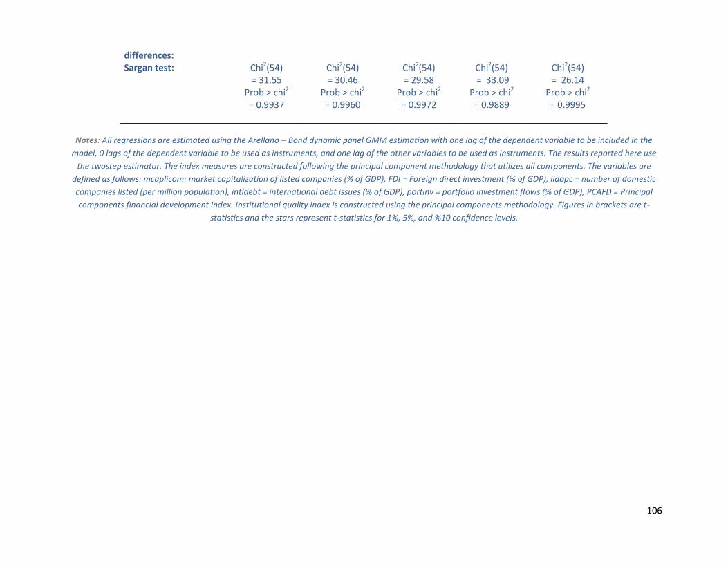
106
differences: Sargan test: Chi2(54)
= 31.55 Chi2(54) = 30.46
Chi2(54) = 29.58
Chi2(54) = 33.09
Chi2(54) = 26.14
Prob > chi2 = 0.9937
Prob > chi2 = 0.9960
Prob > chi2 = 0.9972
Prob > chi2 = 0.9889
Prob > chi2 = 0.9995
Notes: All regressions are estimated using the Arellano – Bond dynamic panel GMM estimation with one lag of the dependent variable to be included in the
model, 0 lags of the dependent variable to be used as instruments, and one lag of the other variables to be used as instruments. The results reported here use
the twostep estimator. The index measures are constructed following the principal component methodology that utilizes all components. The variables are
defined as follows: mcaplicom: market capitalization of listed companies (% of GDP), FDI = Foreign direct investment (% of GDP), lidopc = number of domestic
companies listed (per million population), intldebt = international debt issues (% of GDP), portinv = portfolio investment flows (% of GDP), PCAFD = Principal
components financial development index. Institutional quality index is constructed using the principal components methodology. Figures in brackets are t-
statistics and the stars represent t-statistics for 1%, 5%, and %10 confidence levels.
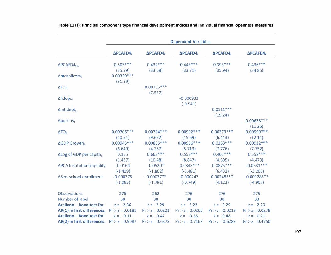
107
Table 11 (f): Principal component type financial development indices and individual financial openness measures
Dependent Variables
∆PCAFD4t ∆PCAFD4t ∆PCAFD4t ∆PCAFD4t ∆PCAFD4t
∆PCAFD4t-1 0.503*** 0.432*** 0.443*** 0.393*** 0.436*** (35.39) (33.68) (33.71) (35.94) (34.85) ∆mcaplicomt 0.00339*** (31.59) ∆FDIt 0.00756*** (7.557) ∆lidopct -0.000933 (-0.541) ∆intldebtt 0.0111*** (19.24) ∆portinvt 0.00678*** (11.25) ∆TOt 0.00706*** 0.00734*** 0.00992*** 0.00373*** 0.00999*** (10.51) (9.652) (15.69) (6.443) (12.11) ∆GDP Growtht 0.00945*** 0.00835*** 0.00936*** 0.0153*** 0.00922*** (6.649) (4.267) (5.713) (7.776) (7.752) ∆Log of GDP per capitat 0.155 0.663*** 0.553*** 0.401*** 0.558*** (1.437) (10.48) (8.847) (4.395) (4.479) ∆PCA Institutional quality -0.0164 -0.0520* -0.0343*** 0.0875*** -0.0531*** (-1.419) (-1.862) (-3.481) (6.432) (-3.206) ∆Sec. school enrollment -0.000375 -0.000777* -0.000247 0.00248*** -0.00128*** (-1.065) (-1.791) (-0.749) (4.122) (-4.907) Observations 276 262 276 276 275 Number of label 38 38 38 38 38 Arellano – Bond test for AR(1) in first differences: Arellano – Bond test for AR(2) in first differences:
z = -2.36 Pr > z = 0.0181
z = -0.11 Pr > z = 0.9087
z = -2.29 Pr > z = 0.0223
z = -0.47 Pr > z = 0.6378
z = -2.22 Pr > z = 0.0265
z = -0.36 Pr > z = 0.7167
z = -2.29 Pr > z = 0.0219
z = -0.48 Pr > z = 0.6283
z = -2.20 Pr > z = 0.0278
z = -0.71 Pr > z = 0.4750
108
Sargan test: Chi2(54) = 32.86
Chi2(54) = 30.86
Chi2(54) = 35.34
Chi2(54) = 32.90
Chi2(54) = 35.71
Prob > chi2 = 0.9898
Prob > chi2 = 0.9953
Prob > chi2 = 0.9768
Prob > chi2 = 0.9896
Prob > chi2 = 0.9740
Notes: All regressions are estimated using the Arellano – Bond dynamic panel GMM estimation with one lag of the dependent variable to be included in the
model, 0 lags of the dependent variable to be used as instruments, and one lag of the other variables to be used as instruments. The results reported here use
the twostep estimator. The index measures are constructed following the principal component methodology that utilizes all components. The variables are
defined as follows: mcaplicom: market capitalization of listed companies (% of GDP), FDI = Foreign direct investment (% of GDP), lidopc = number of domestic
companies listed (per million population), intldebt = international debt issues (% of GDP), portinv = portfolio investment flows (% of GDP), PCAFD4 = Principal
components financial development index excluding the deposit money bank assets to central bank assets ratio. Institutional quality index is constructed using
the principal components methodology. Figures in brackets are t-statistics and the stars represent t-statistics for 1%, 5%, and %10 confidence levels.

109
Table 12: Principal component type financial development and financial openness indices, fixed effects in levels
Dependent Variables
PCABDt PCABD1t PCABMDt PCASMDt PCAFDt PCAFD4t
PCAFOt 0.34825*** (4.22)
0.45020*** (4.67)
0.25722*** (4.86)
0.41546*** (4.24)
0.60681*** (7.36)
0.71384*** (8.00)
TOt -0.00240 (-1.24)
-0.00294 (-1.30)
-0.00130 (-1.23)
0.0098*** (3.73)
0.0009 (0.40)
0.0024 (1.06)
GDP Growtht -0.0171*** (-3.19)
-0.0213*** (-3.40)
-0.00424 (-1.15)
0.00353 (0.37)
-0.00692 (-1.23)
-0.00629 (-1.04)
Log GDP per capitat 1.8698*** (9.67)
2.120*** (9.38)
0.5264*** (4.64)
0.7684*** (2.73)
1.7430*** (8.18)
1.578*** (6.84)
PCA Institutional Quality 0.00538 (0.09)
-0.0023 (-0.03)
-0.129*** (-3.31)
0.06699 (0.66)
0.02515 (0.40)
-0.01507 (-0.22)
Secondary School Enrollment
-0.00186 (-0.88)
-0.0024*** (-0.97)
0.00355*** (2.93)
-0.0078*** (-2.42)
-0.0037** (-1.73)
-0.004** (-1.57)
Constant -15.898*** (-9.78)
-17.96*** (-9.44)
-4.8891*** (-4.84)
-6.7945*** (-2.83)
-15.296*** (-8.18)
-13.850*** (-6.85)
Number of observations:
453 453 401 506 360 360
Number of groups: 51 51 41 56 38 38
R-square: Within: Between: Overall:
0.3530
0.4429 0.4000
0.3526
0.4414 0.3993
0.2299
0.3690 0.3576
0.1935
0.1254 0.1228
0.4927
0.5073 0.4797
0.4774
0.5230 0.4986
F-test for ui=0 F(50,396) = 51.82
F(50,396) = 54.47
F(40,354) = 130.04
F(55,444) = 19.60
F(37, 316) = 44.43
F(37,316) = 52.82
Notes: All regressions are estimated using fixed effects. The index measures are constructed following the principal component methodology that utilizes all
components. The model above includes a higher lag structure, a linear time trend and time dummies. The variables are defined as follows: PCAFO = Principal
components financial openness index, PCABD = Principal components banking sector development index, PCABD1 = Principal components banking sector

110
development index that excludes the deposit money banks to central bank assets ratio, PCABMD = Principal components bond market development index,
PCASMD = Principal components stock market development index, PCAFD = Principal components financial development index, PCFD4 = Principal components
financial development index that excludes the deposit money bank assets to central bank assets ratio. Institutional quality index is constructed using the
principal components methodology. Figures in brackets are t-statistics and the stars represent t-statistics for 1%, 5%, and %10 confidence levels.


