does when you are born matter? - ifs · does when you are born matter? ... 1 introduction it is...
TRANSCRIPT

Does when you are born matter?
The impact of month of birth on children’s
cognitive and non-cognitive skills in England*
A report to the Nuffield Foundation by
Claire Crawford, Lorraine Dearden and Ellen Greaves
(Institute for Fiscal Studies)
November 2011
Copy-edited by Judith Payne
(ISBN: 978-1-903274-87-3)
* The authors are very grateful to the Nuffield Foundation for funding this work (grant number EDU/36559) and to the Economic and Social Research Council (ESRC) for funding via the Centre for the Microeconomic Analysis of Public Policy at IFS (RES-544-28-0001). The authors would also like to extend particular thanks to Rebecca Allen, Maria Evangelou, Helen Evans, Josh Hillman, Jo Hutchinson, Sandra McNally, Tim Oates, Ingrid School and Caroline Sharp for helpful comments and advice. All views expressed are those of the authors.
The Nuffield Foundation is an endowed charitable trust that aims to improve social well-being in the widest sense. It funds research and innovation in education and social policy and also works to build capacity in education, science and social science research. The Nuffield Foundation has funded this project, but the views expressed are those of the authors and not necessarily those of the Foundation. More information is available at http://www.nuffieldfoundation.org.

© Institute for Fiscal Studies, 2011
2
Executive summary
It is well known that children born at the start of the academic year tend to achieve better exam results,
on average, than children born at the end of the academic year. This matters because educational
attainment is known to have long-term consequences for a range of adult outcomes. But it is not only
educational attainment that has long-lasting effects: there is a body of evidence that emphasises the
significant effects that a whole range of skills and behaviours developed and exhibited during childhood
may have on later outcomes. There is, however, relatively little evidence available on the extent to which
month of birth is associated with many of these skills and behaviours, particularly in the UK.
The aim of this report is to build on this relatively limited existing evidence base by identifying the effect
of month of birth on a range of key skills and behaviours amongst young people growing up in England
today, from birth through to early adulthood. This work will extend far beyond the scope of previous
research in this area – in terms of both the range of skills and behaviours considered, and the ability to
consider recent cohorts of children – enabling us to build up a more complete picture of the impact of
month of birth on children’s lives than has previously been possible. In particular, we consider month of
birth differences in the following outcomes:
national achievement test scores and post-compulsory education participation decisions;
other measures of cognitive skills, including British Ability Scale test scores;
parent, teacher and child perceptions of academic ability;
children’s perceptions of their own well-being, including whether or not they have been bullied;
parent and teacher perceptions of children’s socio-emotional development;
children’s engagement in a range of risky behaviours.
We also consider whether parents respond differently to children born in different months of the year,
particularly in terms of the investments they make in their child’s home learning environment.
To do so, we use simple regression models including month of birth dummies (i.e. a series of variables
indicating whether or not a child was born in a particular month, relative to being born in September)
alongside controls for a range of individual and family background characteristics. Our analysis pieces
together information from three UK cohort studies – the Millennium Cohort Study, the Avon Longitudinal
Study of Parents and Children, and the Longitudinal Study of Young People in England – to enable us to
consider month of birth differences in these outcomes from birth through to early adulthood. All three
data sets contain rich information on the skills and behaviours outlined above. They have also all been
linked to administrative data on national achievement test scores, allowing us to compare month of birth
differences amongst cohort members of these surveys with those based on national cohorts.
In line with previous literature, we find evidence of large and significant differences between August- and
September-born children in terms of their cognitive skills, whether measured using national achievement
tests or alternative indicators such as the British Ability Scales. These gaps are particularly pronounced
when considering teacher reports of their performance; moreover, they are also present when
considering differences in socio-emotional development and engagement in a range of risky behaviours.
The absolute magnitude of these differences decreases as children get older, suggesting that August-
borns are ‘catching up’ with their September-born peers in a variety of ways as the difference in relative
age becomes smaller over time.
Interestingly, these differences in academic performance are reflected in young people’s beliefs about
their own ability and the extent to which they are able to control their own lives, but do not appear to
translate into differences in self-worth, enjoyment or perceived value of school, or expectations of and
aspirations for further and higher education. Children born in August are, however, slightly more likely to
report being unhappy or subject to bullying in primary school than children born in September (although

© Institute for Fiscal Studies, 2011
3
these differences do not persist at older ages). They are also significantly more likely to take vocational
qualifications during college (ages 16–18) and slightly less likely to attend a Russell Group university at
age 19. Given the well-documented differences in returns to academic and vocational qualifications, and
by degree institution, these choices may well mean that August-born children end up with poorer labour
market outcomes than September-born children, as other papers have suggested. This is something we
plan to investigate in future research.
We also identify differences in some forms of parental investment by month of birth, with parents of
August-born children providing a richer home learning environment, on average, than parents of
September-born children, by the age of 5. This provides some evidence to support the notion that parents
appear to be ‘compensating’ for the disadvantages that their August-born children face in school by
spending more time at home helping them learn.
Interestingly, though, with the exception of some evidence of differences by household income in the
choice of academic or vocational qualifications at ages 16–18, there are very few consistent differences by
socio-economic status in the month of birth gradients that we observe, i.e. the gaps between August- and
September-born children tend to be similar for low and high income groups, by mother’s work status, etc.
This suggests that, on the whole, families of higher socio-economic status are not able to overcome the
month of birth penalties that their children face any better than families of lower socio-economic status.
While this report provides new evidence of the existence and magnitude of month of birth gradients
across a whole range of skills and behaviours, it does not consider what might be driving these
differences. There are at least four reasons why we might expect children born in different months to
achieve different outcomes:
they are different ages when they sit the tests;
they start school at different ages;
the amount of schooling they receive prior to assessment differs;
their age relative to others in their class or year group differs.
In ongoing research, we are using a combination of administrative and survey data to try to identify
separately the impact of these drivers on children’s test scores. This will enable us to better understand
the most appropriate policy responses to help summer-born children overcome the disadvantages that
the current education system foists upon them. For example, if it is the age at which children start school
that matters most, then this might have implications for the admissions policies that local authorities
choose to follow. On the other hand, if it is the age at which children sit the tests that matters most, then
this may suggest the need to test children when they are ready (i.e. have multiple testing opportunities)
or to age-adjust their scores in some way. We expect to report the results of this research in 2012.
In future research, we are also planning to use the newly available ‘Understanding Society’ data set to
investigate the long-term impact of month of birth on labour market and other outcomes during
adulthood. This will provide us with greater insight into the extent to which the differences documented
in this report go on to have a real and lasting impact on people’s lives.
© Institute for Fiscal Studies, 2011
4
1 Introduction
It is well known that children born at the start of the academic year tend to achieve better exam results,
on average, than children born at the end of the academic year.1 In England, where the academic year
runs from 1 September to 31 August, this means that children born in the autumn tend to significantly
outperform those born in the summer. Our own previous research (Crawford, Dearden & Meghir, 2007)
found large and persistent differences in both average point scores and the probability that a child
reached the standard expected by the government in nationally set exams, with August-born children
performing significantly worse than their September-born counterparts throughout their school lives. For
example, we found that August-born girls (boys) are 5.5 (6.1) percentage points less likely to achieve five
A*–C grades at GCSE than September-born girls (boys).
Given the importance of educational attainment in determining a range of later-life outcomes – from the
probability of being in work and the wage received, to health issues and criminal activity2 – these
differences, which arise because of the interaction between the month of birth and school admissions
policies,3 have the potential to affect individuals throughout their lives. But it is not only educational
attainment that has long-lasting effects: there is a body of literature that emphasises the significant effects
that a whole range of skills and behaviours developed and exhibited during childhood may have on later
outcomes.4
There are a number of reasons why we might expect month of birth – through the age at which children
start school and sit academic tests – to affect the development of these skills. For example, enjoyment of
school has been found to be correlated not only with later academic performance, but also with
engagement in a range of risky behaviours (including smoking, drinking and cannabis use),5 all of which
may create health costs later in life. Similarly, motivation and perseverance in particular tasks have been
found to be significantly positively associated with adult wages, even after taking differences in
educational attainment into account.6 If consistently being amongst the youngest (and perhaps also the
smallest) in your class affects your enjoyment of school and/or your motivation and determination to do
well (amongst other things), then the month in which you were born may have long-term consequences
far beyond those captured by educational attainment alone.
Despite these (and other) potentially important repercussions, however, there is relatively little evidence
available on the extent to which month of birth is associated with the development of many of these skills
and behaviours, particularly in the UK. In fact, the outcomes that have received most attention to date are
the likelihood of being assessed as having special educational needs and the likelihood of being bullied.
1 See, for example, Fredriksson & Ockert (2005), Bedard & Dhuey (2006), Datar (2006), Puhani & Weber (2007), Black, Devereux & Salvanes (2008), Smith (2009) and Department for Education (2010).
2 For some UK examples, see, for example, Dearden (1999), Feinstein (2002a and 2002b), Blundell, Dearden & Sianesi (2005) and Hammond & Feinstein (2006).
3 More specifically, they may arise because of differences in the age at which children born in different months start school or sit the tests, or because of differences in the amount of schooling they receive prior to the tests, or because they are younger relative to other children in their class or school. Crawford, Dearden & Meghir (2007) provided some evidence on which of these effects drives the month of birth differences that we observe. In work to be published in 2012, we update and extend this analysis using a more robust identification strategy.
4 For recent work in the UK, see Carneiro, Crawford & Goodman (2007), Chowdry, Crawford & Goodman (2009) and Goodman & Gregg (2010).
5 See, for example, Goodman & Gregg (2010).
6 See, for example, Duncan & Dunifon (1998) and Duckworth et al. (2007).

© Institute for Fiscal Studies, 2011
5
In terms of the likelihood of being assessed as having special educational needs (SEN), our own previous
research (Crawford, Dearden & Meghir, 2007) showed that during the first year of primary school (age 5),
very few children have been diagnosed with SEN, so differences by month of birth are small and generally
insignificant. The largest penalties are evident at age 11, when August-born girls are 0.4 percentage
points (25%) more likely to have statemented (i.e. more severe) SEN and 8.1 percentage points (72%)
more likely to have non-statemented (i.e. less severe) SEN than September-born girls. The figures for
boys are slightly smaller in percentage terms.
Department for Education (2010) confirmed these findings and also showed that August-born children
are particularly likely to be identified as having learning difficulties and speech, language and
communication needs, which seems consistent with the hypothesis that children who are relatively young
in their year are being identified as having SEN because they are struggling to keep up with their older
peers. Dhuey & Lipscomb (2010) found similar results for the US, with every additional month of
(relative) age decreasing the likelihood of receiving special education services, particularly those
supporting learning disabilities, by 2–5%. Goodman, Gledhill & Ford (2003) for the UK and Elder &
Lubotsky (2009) for the US also found evidence of a negative relationship between relative age and child
psychiatric disorders.
Interestingly, Sharp (1995) found that differences in SEN labelling are only present when teachers are
asked to assess children according to their needs, suggesting that much of the disparity may be driven by
teacher perceptions of the well-established month of birth differences in educational attainment, rather
than by a genuine difference in needs.
In terms of the likelihood of being bullied, Department for Education (2010) used data from the TellUs
survey to show that August-born children are 5–6 percentage points more likely to be bullied than
September-born children at ages 10, 12 and 14. Similarly, Mühlenweg (2010) used Progress in
International Reading Literacy Study (PIRLS) data for 17 countries and found that the youngest children
in a particular grade are more likely to have been bullied within the past month than the older children
within the same grade.
In terms of the effect of month of birth on other skills and behaviours, Dhuey & Lipscomb (2008)
investigated the likelihood of taking a high-school leadership position (defined as either a sports team
captain or a club president). They found that the relatively oldest students in each cohort are 4–11%
more likely to take a leadership position than the relatively youngest. The relatively older students also
believe that they possess more leadership skill than their younger peers. Mühlenweg, Blomeyer & Laucht
(2011) showed that children entering school at a relatively young age are significantly less persistent and
more hyperactive at age 8, although these effects have disappeared by age 11. They also found that young
school entrants are significantly less able to adapt to change at age 11.
The aim of this report is to build on this relatively limited existing evidence base by identifying the effect
of month of birth on a range of key skills and behaviours amongst young people growing up in England
today, from birth through to early adulthood. This work will extend far beyond the scope of previous
research in this area – in terms of both the range of skills and behaviours considered, and the ability to
consider recent cohorts of children – enabling us to build up a more complete picture of the impact of
month of birth on children’s lives than has previously been possible. In particular, we consider month of
birth differences in the following outcomes:
national achievement test scores and post-compulsory education participation decisions;
other measures of cognitive skills, including British Ability Scale test scores;
parent, teacher and child perceptions of academic ability;
children’s perceptions of their own well-being, including whether or not they have been bullied;
parent and teacher perceptions of children’s socio-emotional development;
children’s engagement in a range of risky behaviours.

© Institute for Fiscal Studies, 2011
6
We also consider whether parents respond differently to children born in different months of the year,
particularly in terms of the investments they make in their child’s home learning environment.
Month of birth differences in these outcomes are of interest for at least two reasons: first, because they
affect the well-being of children at the age at which they are observed; and second, because they have
potentially serious long-term consequences for children’s lives. For example, if children born later in the
year are more likely to be bullied, as previous research has suggested, then that is clearly of concern in
and of itself. If, on the other hand, there are significant differences in young people’s sense of control over
their own lives, simply because of the month in which they were born, then we might be more concerned
about this because of its potential effect on their choices and decisions later in life.
To carry out our analysis, we use a simple regression model including month of birth dummies (i.e. a
series of variables indicating whether or not a child was born in a particular month, relative to being born
in September) and month of interview (to recreate the scenario in which all children are surveyed/tested
on the same date), alongside controls for a range of individual and family background characteristics.
Our analysis pieces together information from three UK cohort studies – the Millennium Cohort Study
(MCS), the Avon Longitudinal Study of Parents and Children (ALSPAC) and the Longitudinal Study of
Young People in England (LSYPE) – to enable us to consider month of birth differences in these outcomes
from birth through to early adulthood. All three data sets contain rich information on the skills and
behaviours outlined above. They have also been linked to administrative data on national achievement
test scores, allowing us to compare month of birth differences amongst cohort members of these surveys
with those based on national cohorts.
This report now proceeds as follows: Chapter 2 discusses in more detail the data sets that we use and the
methodology that we adopt; Chapter 3 presents our results; and Chapter 4 concludes and discusses the
next steps in our research agenda.

© Institute for Fiscal Studies, 2011
7
2 Data and methodology
2.1 Data
As described above, we piece together information from three UK cohort studies to enable us to consider
month of birth differences in a range of skills and behaviours from birth to early adulthood. The three
data sets we use are:
the Millennium Cohort Study;
the Avon Longitudinal Study of Parents and Children;
the Longitudinal Study of Young People in England.
These data sets have all been linked to administrative data comprising national achievement test scores
and school census information held by the Department for Education and known as the National Pupil
Database (NPD). We discuss each of these data sets in turn below.
Millennium Cohort Study
The Millennium Cohort Study (MCS) is a longitudinal study that has followed approximately 18,500
children sampled from all live births in the UK between September 2000 and January 2002.7 The first
survey was conducted when the study child was around 9 months old, with follow-ups to date at ages 3, 5
and 7 years. The MCS provides rich information on both the study child and their parents, including the
standard characteristics available in most longitudinal surveys, such as gender, ethnicity, family income
and parental education. Importantly for our purposes, it also provides interviewer-assessed measures of
cognitive ability, as well as parent and teacher reports of the child’s socio-emotional development, at ages
3, 5 and 7. At age 7, the study children themselves were also asked about various aspects of their lives and
their class teachers were surveyed as well.
Specifically, we consider the following outcomes from the MCS:
national achievement test scores at ages 5 and 7 (see the NPD section below for further details);
scores from the British Ability Scales8 (BAS) – a measure of cognitive ability – at ages 3, 5 and 7;
teacher ratings of the child’s performance in reading, writing and maths at age 7;
parent ratings of whether the child has difficulty with reading, writing and maths at age 7;
parent and teacher reports of the Strengths & Difficulties Questionnaire (SDQ)9 at ages 3, 5 and 7;
child reports of whether they like school and are unhappy at school at age 7;
parent and child reports of whether the child is bullied at age 7;
parent reports of the home learning environment they provide for their child at ages 3, 5 and 7;
whether the parent paid for extra lessons at age 7.
7 For more details on the MCS, see http://www.cls.ioe.ac.uk/studies.asp?section=000100020001.
8 For more details on the BAS, see http://www.gl-assessment.co.uk/health_and_psychology/resources/british_ability_scales/british_ability_scales.asp?css=1.
9 The SDQ is a short behavioural screening questionnaire for children aged between 3 and 16. It comprises five questions in each of five sections, designed to capture emotional symptoms, conduct problems, hyperactivity/inattention, peer relationship problems and pro-social behaviour. Respondents are presented with a series of statements about the child’s behaviour and asked to decide whether the statement is ‘not true’ (receiving a score of 0), ‘somewhat true’ (receiving a score of 1) or ‘certainly true’ (receiving a score of 2). A total SDQ score is calculated by summing the scores from the emotional symptoms, conduct problems, hyperactivity/inattention and peer relationship sections, which we then invert to create a measure of positive rather than negative behaviour.

© Institute for Fiscal Studies, 2011
8
Full details of the construction of each of these variables can be found in Appendix A.
In this report, we focus on children born in England only, for two reasons: first, education is a devolved
issue in the UK and the systems in place in Scotland, Wales and Northern Ireland therefore differ
somewhat from that in England; second, it makes our results more comparable to those in the other
survey data sets that we use. All children in the MCS in England were born between 1 September 2000
and 31 August 2001 and are therefore all in the same academic cohort.
Avon Longitudinal Study of Parents and Children
The Avon Longitudinal Study of Parents and Children (ALSPAC) is a longitudinal study that has followed
the children of around 14,000 pregnant women whose expected date of delivery fell between 1 April
1991 and 31 December 1992, and who were resident in the Avon area of England at that time.10 This
means that ALSPAC cohort members were born in one of three academic years: 1990–91, 1991–92 and
1992–93, i.e. they are up to 10 years older than the children in the MCS.
ALSPAC cohort members and their families have been surveyed via high-frequency postal questionnaires
from the time of pregnancy onwards, with information collected on a wide range of family background
characteristics, including mother’s and father’s education and occupational class, income, housing tenure
and so on. In addition, ALSPAC cohort members have been monitored through a number of hands-on
clinics, during which staff administer a range of detailed physical, psychometric and psychological tests.
This provides us with a series of objective measures of skills and behaviours which are less commonly
available in other survey data sets.
Specifically, we consider the following outcomes from ALSPAC:
national achievement test scores at ages 7, 11 and 16 (see the NPD section below for further details);
child reports of their plans to continue in post-compulsory education at age 14;
child reports of their likelihood of going to university or college at age 14;
scores from the Wechsler Intelligence Scale for Children (WISC)11 – a measure of IQ – at age 8;
scores from two comprehension tests: listening at age 8 and reading at age 9;
teacher ratings of the child’s readiness to transition to secondary school at age 11;
child reports of their perceived scholastic competence and self-worth at age 8;
child reports of whether they like school at age 8;
locus of control score (whether the child believes they control their own destiny) at age 8;
parent and teacher reports of the Strengths & Difficulties Questionnaire between ages 7 and 13;
child reports of whether they are bullied at ages 8 and 10;
child reports of whether they smoke and have ever tried cannabis at age 14;
parent reports of the home learning environment they provide for their child at age 3.
Full details of the construction of each of these variables can be found in Appendix A.
Longitudinal Study of Young People in England
The Longitudinal Study of Young People in England (LSYPE) is a longitudinal study following around
16,000 young people in England who were aged 13/14 (henceforth ‘aged 14’) in 2003–04 and are all in
10 For more details on the ALSPAC data resource, see http://www.bristol.ac.uk/alspac/sci-com/.
11 WISC is a measure of IQ comprising five verbal tests (information, similarities, arithmetic, vocabulary and comprehension) and five performance tests (picture completion, coding, picture arrangement, block design and object assembly), which are combined to give a total IQ score (see Wechsler, Golombok & Rust (1992)).

© Institute for Fiscal Studies, 2011
9
the same academic cohort. This means that they were born between 1 September 1989 and 31 August
1990 and are thus slightly older than the sample of young people in ALSPAC. Data have been collected
annually, with six waves currently available, which means that we can observe outcomes for these young
people up to age 18/19 (henceforth ‘age 19’).
The LSYPE collects data on the characteristics of a large sample of today’s teenagers and their families,
including standard things such as gender, ethnicity, family income and parental education, alongside
detailed information on the attitudes and aspirations of children towards education, and engagement in a
range of risky behaviours, throughout their teenage years.
Specifically, we consider the following outcomes from the LSYPE:
national achievement test scores at ages 11, 14 and 16 (see the NPD section below for further
details);
child reports of their plans to continue in post-compulsory education at age 14;
child reports of how likely they are to apply to university from ages 14 to 19;
actual post-compulsory education decisions, including participation in further and higher education;
child reports of their beliefs in their own ability and whether they find school valuable at age 14;
child reports of whether they like school and ever play truant at age 14;
locus of control score (whether the child believes they control their own destiny) at age 15;
child reports of whether they are bullied at ages 14 to 17;
child reports of whether they smoke at ages 14 and 16;
child reports of whether they drink regularly and have ever tried cannabis from ages 14 to 18;
whether the parent paid for extra lessons in academic subjects at ages 14, 15 and 16.
Full details of the construction of each of these variables can be found in Appendix A.
National Pupil Database
The National Pupil Database (NPD) combines data on national achievement test results at the end of each
curriculum period (Key Stage) with (limited) pupil and school characteristics, such as eligibility for free
school meals and special educational needs status, available from the annual (now termly) school
census.12 It is a statutory requirement for all state-funded (and partially state-funded) schools in England
to provide this information; the data are therefore accurate and reliable.
All children in England are assessed at ages 5, 7, 11, 16 and 18. At the end of their first year of school (age
5), pupils are assessed by their teachers on the basis of personal, social and emotional development;
communication, language and literacy; problem solving, reasoning and numeracy; knowledge and
understanding of the world; physical development; and creative development. At age 7, pupils are
assessed on the basis of reading, writing, speaking and listening, maths and science. At the end of primary
school (age 11), they are assessed and tested in English, maths and science. At the end of compulsory
education (age 16), pupils take exams in a range of subjects – usually around 10 in total – including
English, maths and science, which lead to General Certificate of Secondary Education (GCSE) or equivalent
qualifications. These are high-stakes exams that are often used to assess pupils’ ability to continue into
post-compulsory education. The government’s target is for all pupils to achieve at least five A*–C grades
at this level.
As described above, these test results have been linked into each of our survey data sets where possible.
This means that we have access to test results at ages 5 and 7 in the MCS, at ages 7, 11 and 16 in ALSPAC,
and at ages 11, 16 and 18 in the LSYPE. Due to differences in modes of assessment at different ages and
12 For more information on the NPD, see http://nationalpupildatabase.wikispaces.com/.

© Institute for Fiscal Studies, 2011
10
dates, the tests linked to the MCS were all assessed by teachers, while those in ALSPAC and the LSYPE
were all externally examined. In each case, we calculate average point scores for a selection of tests taken
at a particular age and standardise each within sample to have a mean of 0 and a standard deviation of 1
(see Appendix A for full details); this allows us to compare more easily the magnitude of the month of
birth differences that we observe from a variety of tests measured on different scales.
2.2 Methodology
To estimate the impact of month of birth on a wide range of skills and behaviours, we adopt simple linear
regression models of the following form:
yi = αi + δMOBi + λMOIi + βxi + εi
where y is the outcome of interest, MOB is a series of binary (dummy) variables indicating whether the
child is born in a particular month (the omitted month being September), MOI indicates the month in
which the survey interview took place (entered linearly) and x is a vector of individual characteristics.
When we consider whether the effect of month of birth varies by subgroup, we interact the month of birth
dummies with the variable(s) indicating the relevant subgroup of interest (e.g. income quintile).
For continuous outcomes (such as standardised average point scores), we use ordinary least squares
(OLS) regression models. In each case, the coefficients on the month of birth dummy variables are
interpreted as the effect of being born in that particular month, relative to September, in standard
deviations (where a coefficient of 0.2, for example, is equivalent to 20% of a standard deviation). For
binary outcomes (such as whether the young person is ever bullied), we use probit regression models. As
the coefficients from these models are difficult to interpret, we present percentage point impacts in the
figures in Chapter 3, which can be interpreted as marginal effects. For example, a 5 percentage point
impact would be equivalent to moving from a baseline of 26% to 31%, or from 57% to 62%. In all models,
we account for the survey design and non-random attrition where possible.13
The month of birth dummies are our primary characteristics of interest. In this report, we focus on the
effect of being born in August relative to September, but full details of the effects of being born in each
month relative to September can be found in our online appendix.14
While most surveys make some attempt to stagger interviews by age, children born in August and
September tend to be closer in age at the time of most survey interviews than they are when they sit
national achievement tests. An example of this phenomenon is shown in Figure 2.1, in which the solid
vertical lines represent the average age in days at which August- and September-born children were
interviewed for the Wave 3 (age 5) MCS survey, while the dashed lines represent the average age in days
at which they were assessed for the Foundation Stage Profile (FSP). The solid lines are clearly closer
together than the dashed lines, highlighting that the average difference in age in days is larger for the
national achievement tests than for the survey interviews.
To recreate the scenario in which all children are surveyed/tested on the same date, therefore, we
additionally control for month of interview in all regression models using outcomes derived from survey
data (i.e. all outcomes other than those based on national achievement test scores). This ensures that all
13 Wave-specific survey weights that account for non-random attrition as well as the probability of selection for the survey are provided for the MCS and the LSYPE. We also account for the stratification of the MCS and LSYPE survey designs and the clustering of young people in the LSYPE within schools. No such weights are provided for the ALSPAC survey, and the simple random sampling survey design requires no adjustment.
14 http://www.ifs.org.uk/docs/appendix_mob.pdf.

© Institute for Fiscal Studies, 2011
11
of our results, considering different skills and behaviours, taken at different ages and from a variety of
different sources, are comparable.
Figure 2.1 Age in days at MCS Wave 3 (age 5) interview and at Foundation Stage Profile assessment
Notes: Solid vertical lines show mean age at Wave 3 interview. Dashed lines show mean age at FSP.
Finally, some studies have highlighted differences in the number of children born in different months,
particularly just either side of the academic year cut-off, and in the characteristics of the parents of these
children.15 In our analysis, we find very little evidence of such differences16 (see Appendix B), but to
ensure that the individuals we are comparing are as similar as possible – as well as to improve the
precision of our estimates – we include a variety of individual and family background characteristics in
our regression models as well (see Appendix C for full details of the construction of these variables).
15 See, for example, Buckles & Hungerman (2008) and Gans & Leigh (2009).
16 Neither do Dickert-Conlin & Elder (2010).
0
.005
.01
.015
Density
1700 1800 1900 2000 2100 2200Age in days
August born September born
Note: solid lines show the mean age at wave 3 interview, dashed lines show mean age at FSP.

© Institute for Fiscal Studies, 2011
12
3 Results
In this chapter, we document the differences in outcomes between children born in September, at the
start of the academic year, and children born in August, at the end of the academic year. We group related
sets of factors together and examine how the August–September differential changes throughout
childhood, using comparable factors from the Millennium Cohort Study (MCS), the Avon Longitudinal
Study of Parents and Children (ALSPAC) and the Longitudinal Study of Young People in England (LSYPE).
Specifically, we consider differences in:
national achievement test scores and post-compulsory education participation (Section 3.1);
other measures of cognitive skills (Section 3.2);
parent, teacher and child perceptions of academic ability (Section 3.3);
children’s perceptions of their own well-being, including whether or not they are bullied (Section
3.4);
parent and teacher perceptions of children’s socio-emotional development (Section 3.5);
risky behaviours (Section 3.6);
parental investments in the home learning environment (Section 3.7).
Underlying these results are simple regression models of the kind outlined in Section 2.2, which include
children born in all months of the year, alongside a set of controls for month of interview, plus a range of
individual and family background characteristics. Full results from these models can be found in our
online appendix.17
3.1 Educational attainment
This section documents differences in national achievement test scores from age 5 to age 16,18 as well as
differences in aspirations for and participation in further and higher education. Figure 3.1 presents the
differences in standardised average point scores between August- and September-born children, which
are reported in standard deviations.19 As an example of how to interpret these figures, MCS children born
in August score, on average, nearly 80% of a standard deviation lower in the Foundation Stage Profile
than MCS children born in September. This gap is similar to that found in earlier work using national
cohorts (e.g. Crawford, Dearden & Meghir, 2007; henceforth CDM 2007) and to the difference in test
scores between children born to mothers with a degree compared with mothers having no qualifications.
In line with previous work (e.g. CDM 2007), the absolute magnitude of this gap decreases over time,
falling to just over half a standard deviation at age 7 (KS1), 35% of a standard deviation at age 11 (KS2)
and 15% of a standard deviation at age 16 (KS4). Again, these figures are similar to those found using
national cohorts (CDM 2007).
17 http://www.ifs.org.uk/docs/appendix_mob.pdf.
18 See Section 2.1 and Appendix A for further details of the content and construction of each of these outcomes.
19 To provide some sense of the magnitude of these differences, one standard deviation in the Foundation Stage Profile (age 5) is roughly equal to a difference of 20 points; at Key Stage 1 (age 7), it is roughly equal to around 7 points, or the difference between being awarded a Level 2C and a Level 2A; at Key Stage 2 (age 11), it is roughly equal to around 6 points, or the difference between being awarded the government’s expected level (Level 4) and above the expected level (Level 5); at Key Stage 3 (age 14), it is roughly equal to around 6 points, or the difference between being awarded the government’s expected level (Level 5) and above the expected level (Level 6); at Key Stage 4 (age 16), it is roughly equal to around 100 points, or the difference between getting eight C grades and eight A grades at GCSE.

© Institute for Fiscal Studies, 2011
13
Figure 3.1 National achievement test scores: performance of August-born children relative to September-born children
Notes: Error bars represent 95% confidence intervals. Scores have been standardised within sample to have a mean of 0 and a standard deviation of 1.
Figure 3.2 Aspirations for and participation in post-compulsory education: beliefs and actions of August-born children relative to September-born children
Note: Error bars represent 95% confidence intervals.
-1.1
-1.0
-0.9
-0.8
-0.7
-0.6
-0.5
-0.4
-0.3
-0.2
-0.1
0.0
FSP KS1 KS1 KS2 KS2 KS3 KS4 KS4
Stan
dar
d d
evi
atio
ns
KS1
KS1
KS2
-10
-5
0
5
10
15
Plans full-time education (age 14)
Plans full-time education (age 14)
In full-time education (age 17)
Vocational course
(age 17)
Academic course
(age 17)
Pe
rce
nta
ge p
oin
ts
Plans full-time education (age 14)
Plans full-time education (age 14)
MCS
ALSPAC
LSYPE
ALSPAC
LSYPE

© Institute for Fiscal Studies, 2011
14
Figures 3.2 and 3.3 show how these differences translate into young people’s aspirations for and
participation in further and higher education respectively. Figure 3.2 shows that there are no significant
differences between young people born in August and September in terms of their likelihood of planning
to stay in full-time education at age 14. August- and September-born children also overestimate their
chances of staying on in full-time education by roughly equivalent amounts, as there is no difference
between the proportions participating in post-compulsory education at age 17: around 86% of August-
and September-born children in the LSYPE believe they will stay in post-compulsory education when
asked about their expectations at age 14, but only 73% actually participate at age 17.
However, conditional on being in full-time education post-16, those born in August are significantly more
likely to be studying for vocational qualifications (by just over 7 percentage points) and slightly less likely
to be studying for academic qualifications than those born in September (although this estimate is not
significantly different from zero). Given the well-known differences in returns to academic and vocational
qualifications, on average, this suggests that the choices made by (or forced upon) young people born
later in the year may lead to long-run differences in labour market outcomes (e.g. wages). Interestingly,
these differences between the proportions of young people taking academic and vocational qualifications
are driven by individuals from low income groups,20 suggesting that it is these groups who are most likely
to suffer the long-term consequences of being born later in the year. The extent of month of birth
differences in longer-term outcomes is something we plan to investigate further in future research.21
Figure 3.3 shows how the August–September gap in expectations of, applications to and participation in
higher education evolves over time. The magnitude and significance of this gap vary, but suggest that,
amongst LSYPE cohort members, those born in August are less likely to think that they are ‘very likely’ to
apply to university through their teenage years than those born in September, with estimates ranging
from 3.5 to 6.7 percentage points less likely.22 Interestingly, the proportion of young people who believe
they are ‘very likely’ to apply to university rises as they get older, while the proportion of young people
who believe that they are only ‘likely’ to apply falls, as some become more likely and others less likely to
think that they will apply to university (see Figures D.1 and D.2 in Appendix D). This is presumably
because, as young people age, they obtain more accurate information about their educational attainment
and wider circumstances, and their expectations of higher education become more realistic.
Thinking now about differences in actual participation in higher education, Figure 3.3 shows that August-
born pupils are just over 2 percentage points less likely than September-born pupils to go to university at
age 19, although this estimate is not significantly different from zero; this is very similar to the difference
identified using national data (e.g. CDM 2007), in which the larger sample sizes mean that the estimate is
significant. They are also slightly less likely to attend a Russell Group institution – a group of high-status,
research-intensive universities, whose degrees tend to earn graduates higher average wages than degrees
from other institutions23 – again suggesting that month of birth might have consequences that last beyond
formal education and into adulthood, something that we plan to investigate further in future work.
20 To investigate this issue, we reran the regressions, interacting the month of birth dummies with variables indicating the income quintile to which young people belong. These results are available from the authors on request.
21 We plan to use the newly available UK data set ‘Understanding Society’ to investigate the long-term impact of month of birth on labour market and a range of social outcomes during adulthood.
22 The results for the ALSPAC sample suggest that those born in August are actually slightly more likely to think that they are very
likely to apply to university, but this finding is very imprecisely estimated and not statistically significant.
23 See, for example, Chevalier & Conlon (2003).

© Institute for Fiscal Studies, 2011
15
Figure 3.3 Aspirations for and participation in higher education: beliefs and actions of August-born children relative to September-born children
Notes: Error bars represent 95% confidence intervals. Being ‘very likely’ to apply for university at ages 18 and 19 also
includes individuals who have already applied, and at age 19 also includes those who have already started university.
3.2 Other measures of cognitive skills
Figure 3.4 presents differences in other measures of cognitive skills for members of the MCS and ALSPAC,
on the same scale as Figure 3.1 above. Because we control for the month in which children are
interviewed (see Section 2.2 for further details), we are able to compare the month of birth differences in
these measures with those found in national achievement tests, hopefully providing us with a greater
understanding of the extent to which August-born children may be being penalised by not being able to
access a curriculum designed to help them pass these tests.
As was the case in Figure 3.1, the gap in performance between August- and September-born children is
largest at younger ages, with children born in August scoring, on average, nearly 90% of a standard
deviation lower than children born in September on the British Ability Scale at age 3. Thereafter, the
August–September gap declines in absolute magnitude, just as it did for the national achievement tests,
with the differences in BAS scores at ages 5 and 7 (and IQ at age 8) around 10% of a standard deviation
lower than the corresponding gaps in Key Stage tests shown in Figure 3.1.
The August–September differences in comprehension tests taken at ages 8 and 9 also suggest smaller
gaps in cognitive skills than either the Key Stage 1 or Key Stage 2 tests (the closest comparisons). One
potential explanation is that September-born children benefit more from time in school (including the
possibility of ‘teaching to the test’) than August-born children, providing some explanation for why the
gaps are greater in national achievement tests than in other measures of cognitive skills.
-15
-10
-5
0
5
10
15
20
V likely to apply
(age 14)
V likely to apply
(age 14)
V likely to apply
(age 16)
V likely to apply
(age 17)
V likely to apply
(age 18)
V likely to apply
(age 19)
Goes to university (age 19)
Russell Group
university (age 19)
Pe
rce
nta
ge p
oin
ts
V likely to apply (age 14)
V likely to apply (age 14)
ALSPAC
LSYPE

© Institute for Fiscal Studies, 2011
16
Figure 3.4 Other measures of cognitive skills: performance of August-born children relative to September-born children
Notes: Error bars represent 95% confidence intervals. Scores have been standardised within sample to have a mean of 0 and a standard deviation of 1. WOLD and NARA are measures of listening and reading comprehension respectively.
3.3 Parent, teacher and child perceptions of academic ability
The sections above have shown how the performance of August-born children compares with that of
September-born children in various cognitive tests. This section compares how their relative
performance is perceived by parents, teachers and themselves. Figure 3.5 presents differences in parent
and teacher perceptions of the child’s academic ability. It shows that, at age 7, teachers of MCS cohort
members are more likely to report August- than September-born children as being below average in
reading, writing and maths. These differences are substantial: in maths, for example, teachers are 27
percentage points more likely to report August-born students as being below average – which,
considering that they only rate 11% of September-born children as being below average, means that they
are around 2.5 times more likely to rate August-borns as below average.
Interestingly, the parents of August-born children do not appear to be as concerned about their academic
performance as the child’s teacher at the same age: for example, they are only slightly more likely to
report that their child has difficulty with reading than the parents of September-born children, and these
estimates are not significantly different from zero. They are, however, nearly 10 percentage points more
likely to report that their child has difficulty with writing, and 13 percentage points more likely to report
difficulties with maths, although both estimates are significantly lower than the gaps reported by the
child’s class teacher. It is not clear why there should be such stark differences between parent and
teacher reports. One possibility is that teachers are more explicitly comparing children’s performance
within their class or year group, while parents are comparing them with a wider group of individuals,
potentially including other siblings at the same age. Interestingly, it does not seem to be the case that
parents are simply over-optimistic about their child’s academic performance: in fact, parents are more
likely to report that their child has difficulty with reading, writing or maths than their teachers are to
report them as being below average in the same subjects (see Table D.1 in Appendix D for details).
-1.1
-1.0
-0.9
-0.8
-0.7
-0.6
-0.5
-0.4
-0.3
-0.2
-0.1
0.0 BAS (age 3) BAS (age 5) BAS (age 7) IQ (age 8) WOLD (age 8) NARA (age 9)
Stan
dar
d d
evi
atio
ns
BAS (age 3)
NARA (age 9) ALSPAC
MCS

© Institute for Fiscal Studies, 2011
17
Figure 3.5 Parent and teacher perceptions of academic ability: performance of August-born children relative to September-born children
Note: Error bars represent 95% confidence intervals.
Figure 3.6 Child’s perception of themselves and value of school: August-born children relative to September-born children
Notes: Error bars represent 95% confidence intervals. Scales have been standardised within sample to have a mean of 0 and a standard deviation of 1.
-30
-20
-10
0
10
20
30
40
Teacher: below
average in reading
Teacher: below
average in writing
Teacher: below
average in maths
Parent: difficulty reading
Parent: difficulty writing
Parent: difficulty in
maths
Teacher: ready for
secondary school
Pe
rce
nta
ge p
oin
ts
Parent: difficulty writing
Teacher: ready for secondary school
-0.5
-0.4
-0.3
-0.2
-0.1
0.0
0.1
0.2
Scholastic competence
(age 8)
Ability beliefs (age 14)
Self-worth (age 8)
Locus of control (age 8)
Locus of control (age 15)
Value of school
(age 17)
Stan
dar
d d
evi
atio
ns
Self-worth (age 8)
Value of school (age 17)
MCS
ALSPAC
ALSPAC
LSYPE

© Institute for Fiscal Studies, 2011
18
There are also substantial differences between children born in August and children born in September in
terms of whether their teacher thinks they are ‘very ready’ for secondary school (reported at age 11):
teachers report 63% of September-born children as being very ready, compared with just 49% of August-
born children, a difference of over 14 percentage points. This highlights the difficulties that August- and
summer-born children more generally are likely to experience when making the transition from primary
to secondary school, and suggests that additional support might be needed for these children during this
transition period.
Their lower performance on cognitive tests also appears to translate into the perceptions that August-
born children have about their own academic ability. Figure 3.6 shows that children born in August score
themselves significantly lower on a scholastic competence scale at age 8 and an ability beliefs scale at age
14 than children born in September. Interestingly, however, these perceptions of their academic ability
do not appear to translate into significantly lower self-worth more generally. There is also no evidence
that August-born children find school less valuable than their September-born counterparts.
There are, however, some differences in young people’s locus of control, with August-born children
significantly more likely to have an external locus of control, i.e. to believe that their own actions do not
affect what happens to them, at both age 8 (observed in the ALSPAC sample) and age 15 (observed in the
LSYPE sample). Given evidence linking children’s locus of control to later education and labour market
outcomes24, these results again suggest that month of birth may have consequences that last into
adulthood, something that we plan to investigate in future research.
3.4 Perceptions of well-being of young person
We saw in Section 3.3 that while children born in August had lower perceptions of their own academic
ability than children born in September, those differences did not translate into differences in self-worth
or the value they attached to schooling. In this section, we consider whether children born in August
enjoy school less or are bullied more than older children in their year.
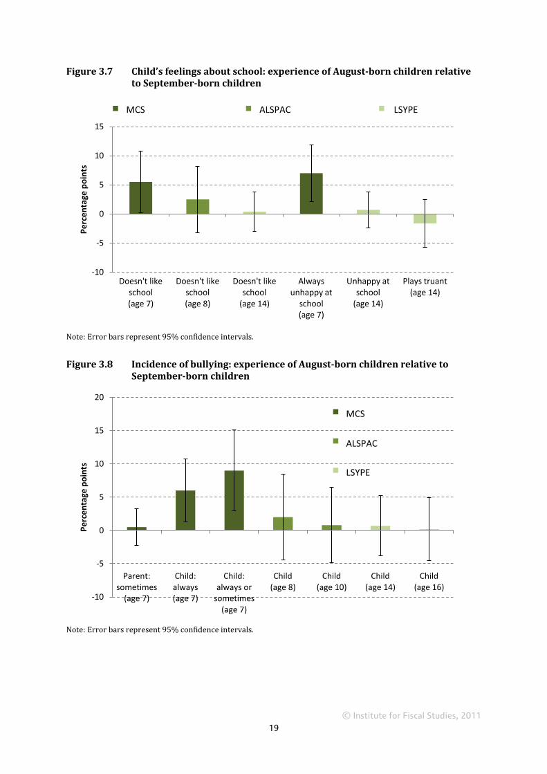
Figure 3.7 shows that, at age 7, August-born children in the MCS are around 5 percentage points more
likely to report not liking school than September-born children – an increase of around one-third relative
to the base of 14% of September-born children that report not liking school (see Table D.1 in Appendix D)
– although these differences are not replicated amongst ALSPAC cohort members at age 8 or amongst
LSYPE cohort members at age 14. August-borns are also significantly more likely to report that they are
unhappy at school than September-borns at age 7, but again this is not replicated in self-reported
measures at age 14. This suggests that while there may be differences in children’s feelings about school
by month of birth at younger ages, these gaps do not persist throughout their school careers.
There is a more mixed picture in terms of differences in the likelihood of being bullied at various ages.
Figure 3.8 shows that August-born children are 9 percentage points (19%) more likely than September-
born children to report being bullied all or some of the time at age 7 in the MCS. This supports the
findings of previous research in this area (e.g. Department for Education, 2010; Mühlenweg, 2010), but is
in contrast to the results based on parent reports in the MCS at the same age, which suggest that there is
no difference in the likelihood of being bullied by month of birth. This is an interesting finding and
perhaps suggests that August-born children are not being completely honest with their parents about the
difficulties they are facing at school.
24 See, for example, Osborne Groves (2005) or Cebi (2007).
© Institute for Fiscal Studies, 2011
19
Figure 3.7 Child’s feelings about school: experience of August-born children relative to September-born children
Note: Error bars represent 95% confidence intervals.
Figure 3.8 Incidence of bullying: experience of August-born children relative to September-born children
Note: Error bars represent 95% confidence intervals.
-10
-5
0
5
10
15
Doesn't like school (age 7)
Doesn't like school (age 8)
Doesn't like school
(age 14)
Always unhappy at
school (age 7)
Unhappy at school
(age 14)
Plays truant (age 14)
Pe
rce
nta
ge p
oin
ts
Doesn't like school (age 7) Doesn't like school (age 8) Plays truant (age 14)
-10
-5
0
5
10
15
20
Parent:
sometimes (age 7)
Child: always (age 7)
Child:
always or sometimes
(age 7)
Child
(age 8)
Child
(age 10)
Child
(age 14)
Child
(age 16)
Pe
rce
nta
ge p
oin
ts
Child: always (age 7)
Child (age 8)
Child (age 14)
ALSPAC MCS LSYPE
ALSPAC
LSYPE
MCS

© Institute for Fiscal Studies, 2011
20
The findings based on child-reported bullying at age 7 in the MCS are also somewhat at odds with those
based on child-reported bullying at ages 8 and 10 in ALSPAC and at age 14 onwards in the LSYPE. One
possible explanation is that this problem is at its worst when the difference in relative age is largest and
decreases over time as the difference in relative age falls; this explanation is likely to be less relevant for
the ALSPAC cohort at age 8, although it must be remembered that this is not a nationally representative
sample.
3.5 Socio-emotional development
It is clear that, on the basis of tests taken at the same point in time, the cognitive skills of August-born
children tend to be significantly lower, on average, than those of September-born children. It is also clear
that these differences are mirrored in the beliefs that young people hold about their own ability, but not
their well-being more generally, particularly not at older ages. In this section, we consider whether there
is any evidence of differences in their socio-emotional development. Figure 3.9 reports gaps in the
reversed scores of August- and September-born children in terms of the Strengths and Difficulties
Questionnaire, as reported by the child’s parent and class teacher at various ages. It shows that August-
born children tend to have lower scores (i.e. poorer socio-emotional development) than September-born
children, on average, at all ages (although the differences are not statistically significant at older ages
when reported by parents).
Figure 3.9 Socio-emotional development (measured by reversed SDQ score): performance of August-born children relative to September-born children
Notes: Error bars represent 95% confidence intervals. Scores have been standardised within sample to have a mean of 0 and a standard deviation of 1.
Differences in socio-emotional development reported by the child’s class teacher are generally larger in
magnitude than those reported by the child’s parent, perhaps suggesting that teachers are more explicitly
comparing children within their class or academic cohort, while parents may be taking into account a
wider range of peers of different ages in assessing their child’s socio-emotional development. As
discussed in Section 3.3, this also appeared to be the case for differences in academic ability. Differences
between August- and September-born children in terms of socio-emotional development reported by
-0.5
-0.4
-0.3
-0.2
-0.1
0.0
0.1
0.2 Age 3 Age 5 Age 7 Age 7 Age 9 Age 11 Age 13 Age 7 Age 8 Age 11
Stan
dar
d d
evi
atio
ns
Age 3
Age 9
Parent-reported SDQ Teacher-reported SDQ
ALSPAC
MCS

© Institute for Fiscal Studies, 2011
21
both parents and teachers decline over time. This suggests that, as was the case with cognitive skills,
August-born children are ‘catching up’ with their September-born peers in terms of socio-emotional
development as they get older and the difference in relative age declines.
It is also interesting to note that the teacher reports of the August–September differences in socio-
emotional development are significantly larger than those between children born to mothers with a
degree compared with mothers having no qualifications, while the parent reports are no different. This
suggests that teachers are more aware of behavioural differences between children born in different
months than between children from different socio-economic backgrounds, while that does not appear to
be the case for parents.25
3.6 Risky behaviours
In this section, we move on to consider month of birth differences in young people’s engagement in a
range of risky behaviours. Figure 3.10 presents differences in the likelihood of sometimes smoking and
ever having tried cannabis. In the LSYPE, the differences are negative and significant in both cases, with
August-borns over 6 percentage points less likely to smoke and over 8 percentage points less likely to
have tried cannabis than September-borns at age 16. These differences are not replicated in the ALSPAC
sample (where the estimates are close to zero in both cases), but it must be remembered that ALSPAC is
not necessarily a representative group of young people in England, as the cohort members were all born
in the Avon area.
Figure 3.10 Smoking and cannabis use: behaviour of August-born children relative to September-born children
Note: Error bars represent 95% confidence intervals.
25 Results are available from the authors on request.
-20
-15
-10
-5
0
5
10
Age 14 Age 14 Age 16 Age 14 Age 14 Age 15 Age 16 Age 17 Age 18
Pe
rce
nta
ge p
oin
ts
Age 14
Age 14
Smokes sometimes Has ever tried cannabis
ALSPAC
LSYPE

© Institute for Fiscal Studies, 2011
22
Figure 3.11 Alcohol consumption: behaviour of August-born children relative to September-born children
Note: Error bars represent 95% confidence intervals.
Figure 3.11 shows that there are also negative and significant differences between those born in August
and those born in September in terms of the probability of drinking alcohol at least once a week,
particularly during compulsory schooling. At age 14, for example, August-borns are 8 percentage points
less likely than September-borns to drink alcohol regularly. Thereafter, this difference increases slightly
up to age 16 (though not significantly so) and then starts to fall, so that by age 18 it is effectively zero. As
was the case for cannabis usage, and indeed for the academic test results reported in Section 3.1, young
people born in August appear to be ‘catching up’ with their September-born peers over time: in general,
while there is a sizeable difference in engagement in risky behaviours in the mid-teenage years – when
relatively few young people participate (see Table D.1 in Appendix D) – by age 17 or 18 many more
engage in each activity and the gap in participation between those born at the start and end of the
academic year has grown relatively smaller.
3.7 Parental investments
So far, this chapter has documented the sometimes large differences in outcomes – both cognitive and
non-cognitive – between children according to the month in which they were born. In this section, we
consider whether parents respond to the month of birth differences that we and they observe, to provide
their children with correspondingly more or less ‘investment’ of either time or resources in order to aid
their development. The direction of this response is theoretically uncertain: it could be that parents try to
compensate for the differences that they observe, i.e. that parents of August-born children invest more in
order to compensate for the lower performance of their children along a variety of dimensions;
alternatively, it could be that parents of September-born children invest more because they know that
‘skills beget skills’, i.e. that their investment will be more productive because their child has higher skills
to start with. Their response to month of birth differences is thus an empirical question.
-20
-15
-10
-5
0
5
10
Age 14 Age 15 Age 16 Age 17 Age 18
Pe
rce
nta
ge p
oin
ts
Series 1 LSYPE

© Institute for Fiscal Studies, 2011
23
Figure 3.12 Home learning environment: experience of August-born children relative to September-born children
Notes: Error bars represent 95% confidence intervals. Scales have been standardised within sample to have a mean of 0 and a standard deviation of 1.
Figure 3.13 Paying for extra lessons/tuition for child: experience of August-born children relative to September-born children
Note: Error bars represent 95% confidence intervals.
Figure 3.12 presents estimates of the difference in the home learning environment (in terms of reading to
their child, teaching them the alphabet, etc.) provided by parents at ages 3, 5 and 7. At age 3, it is clear
that there is no difference in the home learning environment between children born in August and
-0.20
-0.15
-0.10
-0.05
0.00
0.05
0.10
0.15
0.20
0.25
0.30
Age 3 Age 3 Age 5 Age 7 Stan
dar
d d
evi
atio
ns
Age 3
Age 3
-4
-3
-2
-1
0
1
2
3
4
Age 7 Age 14 Age 15 Age 16
Pe
rce
nta
ge p
oin
ts
Age 7
Age 14
MCS
ALSPAC
LSYPE
MCS

© Institute for Fiscal Studies, 2011
24
children born in September; at ages 5 and 7, however, it appears that the parents of August-born children
provide a richer home learning environment for their children than the parents of September-born
children. This provides some support for the ‘compensating’ hypothesis described above.
It is particularly interesting to note that the greater investment does not occur until after the children
start school, suggesting that it is not until parents are able to compare their child’s performance more
explicitly with that of other children in the same academic cohort that they change their behaviour.
Alternatively, it is plausible that the greater relative age of the September-born children means that they
are more likely to have younger siblings, thus reducing the amount of time parents can spend with these
older children. We do not observe this phenomenon in the MCS cohort, however: those born in September
are not significantly more likely to have a younger sibling than those born in August.26
This change in behaviour does not extend to a difference in the likelihood of paying for additional private
tuition, however, either at age 7 or during the teenage years (see Figure 3.13), with all estimates being
small and not significantly different from zero.
3.8 Summary
To summarise, this chapter has shown that there are large and significant differences between
August- and September-born children in terms of their cognitive skills, whether measured using national
achievement tests or alternative indicators such as the British Ability Scales. These gaps are particularly
pronounced when considering teacher reports of their performance. They are also present when
considering differences in socio-emotional development and engagement in a range of risky behaviours.
In line with other literature (e.g. Crawford, Dearden & Meghir, 2007), the absolute magnitude of these
differences decreases as children get older, suggesting that August-borns are ‘catching up’ with their
September-born counterparts in a variety of ways as the difference in relative age becomes smaller over
time.
Interestingly, these differences in academic performance are reflected in young people’s beliefs about
their own ability and the extent to which they are able to control their own lives, but do not appear to
translate into differences in self-worth, enjoyment or perceived value of school, or expectations of and
aspirations for further and higher education. Children born in August are, however, slightly more likely to
report being unhappy or subject to bullying in primary school than children born in September (although
these differences do not persist at older ages). They are also significantly more likely to take vocational
qualifications during college and slightly less likely to attend a Russell Group university at age 19. Given
the well-documented differences in returns to academic and vocational qualifications, and by degree
institution,27 these choices may well mean that August-born children end up with poorer labour market
outcomes than September-born children, as some papers have suggested.28 This is something we plan to
investigate in future research.
We have also identified differences in some forms of parental investment by month of birth, with parents
of August-born children providing a richer home learning environment, on average, than parents of
September-born children, by the age of 5. This provides some evidence to support the notion that parents
appear to be ‘compensating’ for the disadvantages that their August-born children face in school by
spending more time with them at home.
26 At the age 5 survey, 44% of children born in September have a younger sibling, compared with 41% of children born in August. This difference is not statistically significant, however (the p-value on a two-sided test is 0.201).
27 See, for example, Dearden et al. (2002) and Chevalier & Conlon (2003).
28 See, for example, Bedard & Dhuey (2009), Kawaguchi (2011) or Solli (2011) – although not all papers support these conclusions: see, for example, Black, Devereux & Salvanes (2008) or Dobkin & Ferreira (2010).

© Institute for Fiscal Studies, 2011
25
Finally, with the exception of some evidence of differences by household income in the choice of academic
or vocational qualifications at ages 16–18, there are very few consistent differences by socio-economic
status in the month of birth gradients that we observe, i.e. the gaps between August- and September-born
children tend to be similar for low and high income groups, by mother’s work status, etc.29 This suggests
that, on the whole, families of higher socio-economic status are not able to overcome the month of birth
penalties that their children face any better than families of lower socio-economic status.
29 Further details of these results are available on request from the authors.

© Institute for Fiscal Studies, 2011
26
4 Conclusions and next steps
There is already a sizeable evidence base documenting the relationship between month of birth and
cognitive skills, including educational attainment, in the UK and elsewhere; however, there is relatively
little evidence of the effect of month of birth on other types of skills and behaviours, including non-
cognitive skills. Such differences matter both because they may affect children’s well-being at the time of
observation and because they may have potentially long-lasting consequences for their adult lives. The
aim of this report has been to help fill this evidence gap.
We have made use of three overlapping cohort studies to build up a more complete picture than has
hitherto been possible of the effect of month of birth on a range of key skills and behaviours – including
behaviour at and views of school, post-compulsory education aspirations and choices, engagement in
risky behaviours and wider measures of well-being, such as experience of bullying – amongst young
people growing up in England today, from birth to early adulthood.
In line with previous literature, we have found evidence of large and significant differences between
August- and September-born children in terms of their cognitive skills, whether measured using national
achievement tests or alternative indicators such as the British Ability Scales. These gaps were particularly
pronounced when considering teacher reports of children’s performance; moreover, they were also
present when considering differences in socio-emotional development and engagement in a range of
risky behaviours. The absolute magnitude of each of these differences decreases as children get older,
suggesting that August-borns ‘catch up’ with their September-born peers in a variety of ways as the
difference in relative age becomes smaller over time.
Interestingly, these differences in academic performance are reflected in young people’s beliefs about
their own ability and the extent to which they are able to control their own lives, but do not appear to
translate into differences in self-worth, enjoyment or perceived value of school, or expectations of and
aspirations for further and higher education. Children born in August are, however, slightly more likely to
report being unhappy or subject to bullying in primary school than children born in September (although
these differences do not persist at older ages). They are also significantly more likely to take vocational
qualifications during college and slightly less likely to attend a Russell Group university at age 19. Given
the well-documented differences in returns to academic and vocational qualifications, and by degree
institution, these choices may well mean that August-born children end up with poorer labour market
outcomes than September-born children, as some other papers have suggested.
We have also identified differences in some forms of parental investment by month of birth, with parents
of August-born children providing a richer home learning environment, on average, than parents of
September-born children, by the age of 5. This provides some evidence to support the notion that parents
appear to be ‘compensating’ for the disadvantages that their August-born children face in school by
spending more time with them at home.
Interestingly, though, with the exception of some evidence of differences by household income in the
choice of academic or vocational qualifications at ages 16–18, there are very few consistent differences by
socio-economic status in the month of birth gradients that we observe, i.e. the gaps between August- and
September-born children tend to be similar for low and high income groups, by mother’s work status, etc.
This suggests that, on the whole, families of higher socio-economic status are not able to overcome the
month of birth penalties that their children face any better than families of lower socio-economic status.

© Institute for Fiscal Studies, 2011
27
Next steps
This report has provided new evidence of the existence and magnitude of month of birth gradients across
a whole range of skills and behaviours. It has not, however, considered what might be driving these
differences. There are at least four reasons why we might expect children born in different months to
achieve different outcomes:
age of sitting the test (absolute age) effect: if all children sit exams on the same day, then those
born later in the academic year will always be younger than their peers when taking the tests;
age of starting school effect: perhaps it is not the age at which children sit the test that is important,
but the age at which they start school, i.e. it is their ‘readiness for school’ that matters;
length of schooling effect: if younger children experience fewer terms of schooling prior to the tests
than the older members of their cohort, then this might explain their poorer academic performance;
age position (relative age) effect: under this hypothesis, younger children tend to perform more
poorly not because they are the youngest in absolute terms, but because they are the youngest
relative to others in their class or year group.30
In ongoing research, we are using data from the Millennium Cohort Study and the National Pupil Database
to try to identify separately the impact of each of these four potential drivers on children’s test scores.
This will enable us to better understand the most appropriate policy responses to help summer-born
children overcome the disadvantages that the current education system foists upon them. For example, if
it is the age at which children start school that matters most, then this might have implications for the
admissions policies that local authorities choose to follow. On the other hand, if it is the age at which
children sit the tests that matters most, then this may suggest the need to test children when they are
ready (i.e. have multiple testing opportunities) or to age-adjust their scores in some way. We expect to
report the results of this research in 2012.
In future research, we are also planning to use the newly available ‘Understanding Society’ data set to
investigate the long-term impact of month of birth on labour market and other outcomes during
adulthood. This will provide us with greater insight into the extent to which the differences documented
in this report go on to have a real and lasting impact on people’s lives.
30 The implication is that if all children sat the exam on their birthday (assuming that they also all received the same amount of schooling beforehand), then the scores of the youngest would still not be as high as those of the oldest.

© Institute for Fiscal Studies, 2011
28
Appendix A
Variable Description MCS Foundation Stage Profile (FSP) total score Score from national data. Teacher assessed at the end of
reception year (age 5) along the following components: personal, social and emotional development; communication, language and literacy; mathematical development; knowledge and understanding of the world; physical development; creative development. Summed to create a total raw score and standardised on the whole sample to have mean 0 and standard deviation 1.
KS1 average points score (age 7) Score from national data. Teacher assessed at the end of Key Stage 1 (age 7). The average points score is constructed from assessments in English, maths and science. This score is standardised on the whole sample to have mean 0 and standard deviation 1.
BAS total score (age 3) British Ability Scale, naming vocabulary test. Total score is standardised on the whole sample to have mean 0 and standard deviation 1.
BAS total score (age 5) Created from three components of the British Ability Scale: naming vocabulary, picture similarity and pattern construction. Each component was standardised on the whole sample to have mean 0 and standard deviation 1. An average score was created from these three standardised scores provided at least two components were present.
BAS total score (age 7) Created from three components of the British Ability Scale: word reading, pattern construction and maths. Each component was standardised on the whole sample to have mean 0 and standard deviation 1. An average score was created from these three standardised scores provided at least two components were present.
Teacher rates below average in reading (age 7) Binary variable coded to equal 1 if the child’s teacher reports that the child is ‘below average’ or ‘well below average’ in reading, and 0 otherwise.
Teacher rates below average in writing (age 7) As above, for writing.
Teacher rates below average in maths (age 7) As above, for maths.
Parent states difficulty in reading (age 7) Binary variable coded to equal 1 if the child’s parent reports that the child has ‘some difficulty’ or ‘great difficulty’ in reading, and 0 otherwise.
Parent states difficulty in writing (age 7) As above, for writing.
Parent states difficulty in maths (age 7) As above, for maths.
Parent-reported Strengths and Difficulties Questionnaire (age 3)
Scale created from five questions in each of four dimensions: emotional development, conduct, hyperactivity and relationship with peers. The total score is reversed and standardised on the whole sample to have mean 0 and standard deviation 1.
Parent-reported Strengths and Difficulties Questionnaire (age 5)
As above.
Parent-reported Strengths and Difficulties Questionnaire (age 7)
As above.
Teacher-reported Strengths and Difficulties Questionnaire (age 7)
As above, reported by the teacher.

© Institute for Fiscal Studies, 2011
29
MCS continued Parent paid for additional lessons (age 7) Binary variable coded to equal 1 if the child’s parent
reported paying for extra lessons for the child in reading, writing or maths, and 0 otherwise.
Home learning environment (age 3) Scale created from six questions answered by parents: the frequency of reading to the child and visiting the library (where ‘daily’ corresponded to a score of 7 and ‘less often than once or twice a month’ corresponded to a score of 1); whether they teach the child the alphabet and paint and draw, practise numbers and counting, and sing songs, poems or nursery rhymes with the child (where a positive response corresponded to a score of 1). The total score is standardised on the whole sample to have mean 0 and standard deviation 1.
Home learning environment (age 5) Scale created from four questions answered by parents: the frequency of reading to the child, telling stories, musical activities, and drawing and painting (where ‘daily’ corresponded to a score of 7 and ‘less often than once or twice a month’ corresponded to a score of 1). The total score is standardised on the whole sample to have mean 0 and standard deviation 1.
Home learning environment (age 7) Scale created from four questions answered by parents: the frequency of reading to the child, telling stories, musical activities, and drawing and painting (where ‘daily’ corresponded to a score of 7 and ‘less often than once or twice a month’ corresponded to a score of 1). The total score is standardised on the whole sample to have mean 0 and standard deviation 1.
Child doesn’t like school (age 7) Binary variable coded equal to 1 if the child responds ‘I don’t like it’ to the question ‘How much do you like school?’, and 0 otherwise.
Always unhappy at school (age 7) Binary variable coded equal to 1 if the child responds ‘all of the time’ to the question ‘How often do you feel unhappy at school?’, and 0 otherwise.
Parent reports child is bullied at least several times (age 7)
Binary variable coded equal to 1 if the parent reports that the child has been bullied at school ‘several times’ or ‘many times’, and 0 otherwise.
Child reports always bullied (age 7) Binary variable coded equal to 1 if the child responds ‘all of the time’ to the question ‘How often do other children bully you?’, and 0 otherwise.
Child reports always/sometimes bullied (age 7) Binary variable coded equal to 1 if the child responds ‘all of the time’ or ‘some of the time’ to the question ‘How often do other children bully you?’, and 0 otherwise.
ALSPAC KS1 capped points score Score from national data. Externally assessed at the end of
Key Stage 1 (age 7). The average points score is constructed from assessments in reading, writing and maths. This score is standardised on the whole sample to have mean 0 and standard deviation 1.
KS2 average points score Score from national data. Externally assessed at the end of Key Stage 2 (age 11). The average points score is constructed from assessments in English, maths and science. This score is standardised on the whole sample to have mean 0 and standard deviation 1.
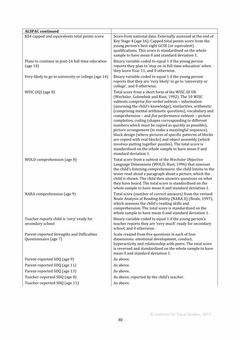
© Institute for Fiscal Studies, 2011
30
ALSPAC continued KS4 capped and equivalents total points score Score from national data. Externally assessed at the end of
Key Stage 4 (age 16). Capped total points score from the young person’s best eight GCSE (or equivalent) qualifications. This score is standardised on the whole sample to have mean 0 and standard deviation 1.
Plans to continue in post-16 full-time education (age 14)
Binary variable coded to equal 1 if the young person reports they plan to ‘stay on in full-time education’ when they leave Year 11, and 0 otherwise.
Very likely to go to university or college (age 14) Binary variable coded to equal 1 if the young person reports that they are ‘very likely’ to go to ‘university or college’, and 0 otherwise.
WISC (IQ) (age 8) Total score from a short form of the WISC-III UK (Wechsler, Golombok and Rust, 1992). The 10 WISC subtests comprise five verbal subtests – information (assessing the child’s knowledge), similarities, arithmetic (comprising mental arithmetic questions), vocabulary and comprehension – and five performance subtests – picture completion, coding (shapes corresponding to different numbers which must be copied as quickly as possible), picture arrangement (to make a meaningful sequence), block design (where pictures of specific patterns of blocks are copied with real blocks) and object assembly (which involves putting together puzzles). The total score is standardised on the whole sample to have mean 0 and standard deviation 1.
WOLD comprehension (age 8) Total score from a subtest of the Wechsler Objective Language Dimensions (WOLD; Rust, 1996) that assesses the child’s listening comprehension: the child listens to the tester read aloud a paragraph about a picture, which the child is shown. The child then answers questions on what they have heard. The total score is standardised on the whole sample to have mean 0 and standard deviation 1.
NARA comprehension (age 9) Total score (number of correct answers) from the revised Neale Analysis of Reading Ability (NARA II) (Neale, 1997), which assesses the child’s reading skills and comprehension. The total score is standardised on the whole sample to have mean 0 and standard deviation 1.
Teacher reports child is ‘very’ ready for secondary school
Binary variable coded to equal 1 if the young person’s teacher reports they are ‘very much’ ready for secondary school, and 0 otherwise.
Parent-reported Strengths and Difficulties Questionnaire (age 7)
Scale created from five questions in each of four dimensions: emotional development, conduct, hyperactivity and relationship with peers. The total score is reversed and standardised on the whole sample to have mean 0 and standard deviation 1.
Parent-reported SDQ (age 9) As above.
Parent-reported SDQ (age 11) As above.
Parent-reported SDQ (age 13) As above.
Teacher-reported SDQ (age 8) As above, reported by the child’s teacher.
Teacher-reported SDQ (age 11) As above.

© Institute for Fiscal Studies, 2011
31
ALSPAC continued Home learning environment (age 3) Scale created from parent reports of frequency of visiting
the library, reading to the child and singing with the child (where ‘nearly daily’ is coded as 4 and ‘never’ is coded as 0) and whether the parent teaches the child colours, the alphabet, numbers, nursery rhymes, songs, and shapes and sizes (where a positive response is coded as 1). Each component is standardised and a scale is created from the total. The scale is then standardised on the whole sample to have mean 0 and standard deviation 1.
Child doesn’t like school (age 8) Binary variable coded to equal 1 if the young person responds ‘not much’ or ‘no’ when asked whether they like school, and 0 otherwise.
Scholastic competence (age 8) A total score created from six items from a shortened form of Harter’s Self-Perception Profile for Children (Harter, 1985), where children responded to questions by ‘posting’ whether the statement was true or not for them in a box. The score is then standardised on the whole sample to have mean 0 and standard deviation 1.
Global self-worth (age 8) A total score created from six items from a shortened form of Harter’s Self-Perception Profile for Children (Harter, 1985), where children responded to questions by ‘posting’ whether the statement was true or not for them in a box. The score is then standardised on the whole sample to have mean 0 and standard deviation 1.
Locus of control (age 8) Total score from a shortened version of the Nowicki–Strickland Internal–External scale (Nowicki & Strickland, 1973) for pre-school and primary children. The score is then standardised on the whole sample to have mean 0 and standard deviation 1. Higher values indicate a more “internal” locus of control.
Victim of bullying (age 8) Derived from a series of questions asked to the child about events that may have happened to them, such as whether they had personal belongings taken from them or been hit / beaten up. Answers to these questions categorised children into being bullied ‘overtly’ or ‘relationally’. We combine these indicators into a single binary variable, coded to equal 1 if the child was bullied in either way, and 0 otherwise.
Victim of bullying (age 10) As above.
Smokes at least 1–6 cigarettes per week (age 14) Binary variable coded to equal 1 if the young person reports that they usually smoke ‘1–6 a week’ or more, and 0 otherwise.
Smokes at least sometimes (age 14) Binary variable coded to equal 1 if the young person reports that they usually smoke ‘sometimes, but less than 1 a week’ or more, and 0 otherwise.
Ever tried cannabis (age 14) Binary variable coded to equal 1 if the young person reports that they have ever tried cannabis, and 0 otherwise.
LSYPE KS2 average points score Score from national data. Externally assessed at the end of
Key Stage 2 (age 11). The average points score is constructed from assessments in English, maths and science. This score is standardised on the whole sample to have mean 0 and standard deviation 1.
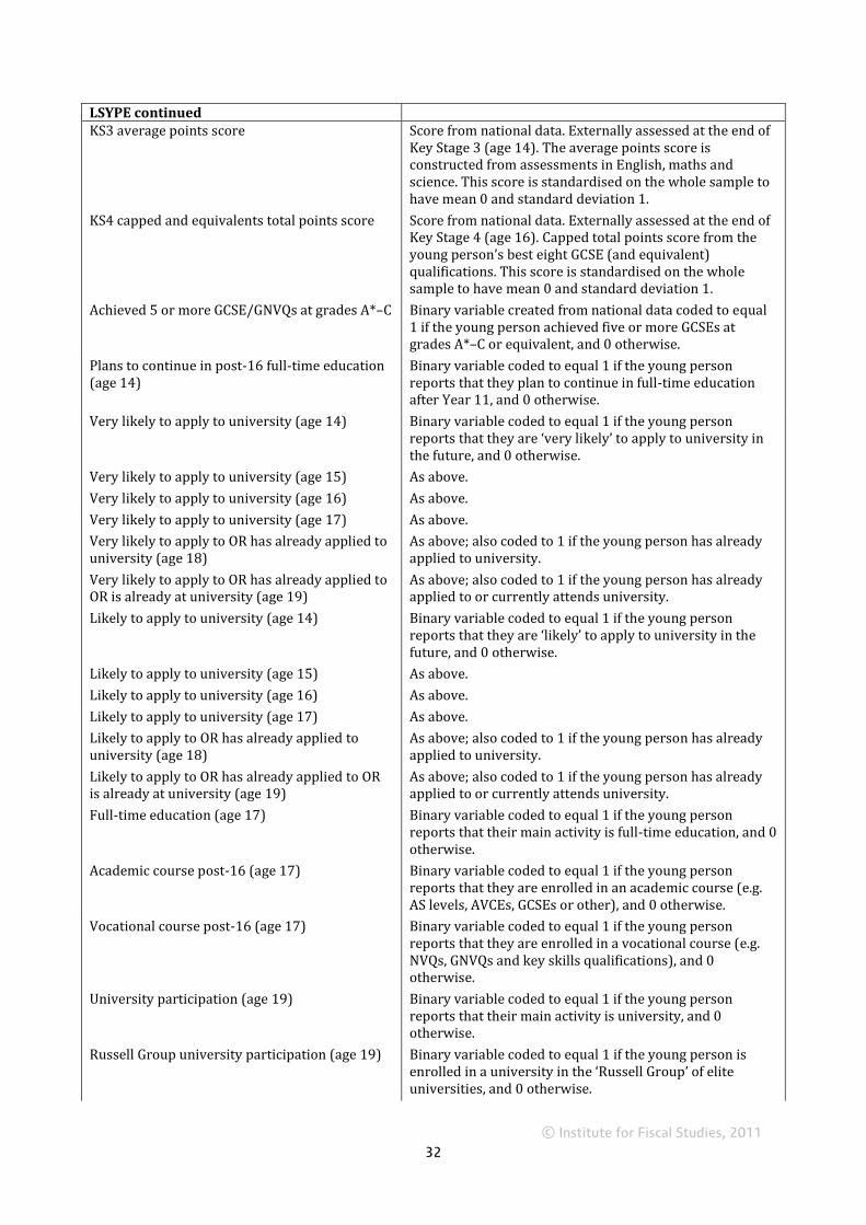
© Institute for Fiscal Studies, 2011
32
LSYPE continued KS3 average points score Score from national data. Externally assessed at the end of
Key Stage 3 (age 14). The average points score is constructed from assessments in English, maths and science. This score is standardised on the whole sample to have mean 0 and standard deviation 1.
KS4 capped and equivalents total points score Score from national data. Externally assessed at the end of Key Stage 4 (age 16). Capped total points score from the young person’s best eight GCSE (and equivalent) qualifications. This score is standardised on the whole sample to have mean 0 and standard deviation 1.
Achieved 5 or more GCSE/GNVQs at grades A*–C Binary variable created from national data coded to equal 1 if the young person achieved five or more GCSEs at grades A*–C or equivalent, and 0 otherwise.
Plans to continue in post-16 full-time education (age 14)
Binary variable coded to equal 1 if the young person reports that they plan to continue in full-time education after Year 11, and 0 otherwise.
Very likely to apply to university (age 14) Binary variable coded to equal 1 if the young person reports that they are ‘very likely’ to apply to university in the future, and 0 otherwise.
Very likely to apply to university (age 15) As above.
Very likely to apply to university (age 16) As above.
Very likely to apply to university (age 17) As above.
Very likely to apply to OR has already applied to university (age 18)
As above; also coded to 1 if the young person has already applied to university.
Very likely to apply to OR has already applied to OR is already at university (age 19)
As above; also coded to 1 if the young person has already applied to or currently attends university.
Likely to apply to university (age 14) Binary variable coded to equal 1 if the young person reports that they are ‘likely’ to apply to university in the future, and 0 otherwise.
Likely to apply to university (age 15) As above.
Likely to apply to university (age 16) As above.
Likely to apply to university (age 17) As above.
Likely to apply to OR has already applied to university (age 18)
As above; also coded to 1 if the young person has already applied to university.
Likely to apply to OR has already applied to OR is already at university (age 19)
As above; also coded to 1 if the young person has already applied to or currently attends university.
Full-time education (age 17) Binary variable coded to equal 1 if the young person reports that their main activity is full-time education, and 0 otherwise.
Academic course post-16 (age 17) Binary variable coded to equal 1 if the young person reports that they are enrolled in an academic course (e.g. AS levels, AVCEs, GCSEs or other), and 0 otherwise.
Vocational course post-16 (age 17) Binary variable coded to equal 1 if the young person reports that they are enrolled in a vocational course (e.g. NVQs, GNVQs and key skills qualifications), and 0 otherwise.
University participation (age 19) Binary variable coded to equal 1 if the young person reports that their main activity is university, and 0 otherwise.
Russell Group university participation (age 19) Binary variable coded to equal 1 if the young person is enrolled in a university in the ‘Russell Group’ of elite universities, and 0 otherwise.

© Institute for Fiscal Studies, 2011
33
LSYPE continued Parent paid for additional academic lessons (age 14)
Binary variable coded to equal 1 if the parent reports paying for extra lessons in English, maths, science or languages, and 0 otherwise.
Parent paid for additional academic lessons (age 15)
As above.
Parent paid for additional academic lessons (age 16)
As above.
Ability beliefs (age 14) Scale created from young person’s response to six questions about academic ability: ‘How good are you at English, maths, science and ICT?’ (where responses ranged from ‘very good’ to ‘not good at all’), and whether they strongly agree, agree, disagree or strongly disagree that they ‘get good marks for my work’ and are ‘good at school work’. For each question, the most positive response was given the highest score, each variable was standardised to have mean 0 and standard deviation 1, and then summed to create a total score. This total score is then standardised on the whole sample to have mean 0 and standard deviation 1.
Usefulness of school (age 14) As above, for three questions relating to the usefulness of school, such as how much the young person agrees with the statements ‘School is a waste of time for me’ and ‘School work is worth doing’.
Value of school (age 17) As above, for five questions relating to the value of school, such as how much the young person agrees with the statements ‘My school work in Year 11 was usually worth doing’ and ‘School has taught me things which would be useful in a job’.
Locus of control (age 15) Total score derived from eight questions relating to how much the young person controls their own destiny, e.g. ‘I can pretty much decide what will happen in my life’, where a higher score means they are more likely to believe they control their own destiny. The score is then standardised on the whole sample to have mean 0 and standard deviation 1. Higher values indicate a more “internal” locus of control.
Young person doesn’t like school (age 14) Binary variable coded to equal 1 if the young person reports that they ‘disagree’ or ‘strongly disagree’ that they like school, and 0 otherwise.
Young person is unhappy at school (age 14) Binary variable coded to equal 1 if the young person reports that they ‘disagree’ or ‘strongly disagree’ that they are happy at school, and 0 otherwise.
High score on bullying scale (age 14) First, a total score was created from five questions on the frequency of different types of bullying reported by the young person. A binary variable was then created equal to 1 if the young person falls in the top 25% of this total score, and 0 otherwise.
High score on bullying scale (age 15) As above.
High score on bullying scale (age 16) As above.
High score on bullying scale (age 17) As above, but created from six questions.
Smokes at least sometimes (age 14) Binary variable coded to equal 1 if the young person reports that they ‘sometimes smoke cigarettes’ or smoke more frequently, and 0 otherwise.
Smokes at least sometimes (age 16) As above.

© Institute for Fiscal Studies, 2011
34
LSYPE continued Drunk alcohol at least once a month for the past 12 months (age 14)
Binary variable coded to equal 1 if the young person reports that they have drunk alcohol ‘at least once a month over past 12 months’ or more frequently, and 0 otherwise.
Drunk alcohol at least once a month for the past 12 months (age 15)
As above.
Drunk alcohol at least once a month for the past 12 months (age 16)
As above.
Drunk alcohol at least once a month for the past 12 months (age 17)
As above.
Drunk alcohol at least once a month for the past 12 months (age 18)
As above.
Ever tried cannabis (age 14) Binary variable coded to equal 1 if the young person reports that they have ever tried cannabis, and 0 otherwise.
Ever tried cannabis (age 15) As above.
Ever tried cannabis (age 16) As above.
Ever tried cannabis (age 17) As above.
Ever tried cannabis (age 18) As above.
Ever plays truant (age 14) Binary variable coded to equal 1 if the young person reports that they have played truant in the past 12 months, and 0 otherwise.
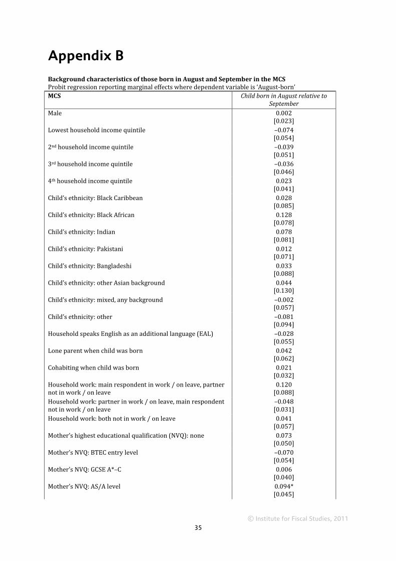
© Institute for Fiscal Studies, 2011
35
Appendix B
Background characteristics of those born in August and September in the MCS Probit regression reporting marginal effects where dependent variable is ‘August-born’
MCS Child born in August relative to September
Male 0.002 [0.023]
Lowest household income quintile –0.074 [0.054]
2nd household income quintile –0.039 [0.051]
3rd household income quintile –0.036 [0.046]
4th household income quintile 0.023 [0.041]
Child’s ethnicity: Black Caribbean 0.028 [0.085]
Child’s ethnicity: Black African 0.128 [0.078]
Child’s ethnicity: Indian 0.078 [0.081]
Child’s ethnicity: Pakistani 0.012 [0.071]
Child’s ethnicity: Bangladeshi 0.033 [0.088]
Child’s ethnicity: other Asian background 0.044 [0.130]
Child’s ethnicity: mixed, any background –0.002 [0.057]
Child’s ethnicity: other –0.081 [0.094]
Household speaks English as an additional language (EAL) –0.028 [0.055]
Lone parent when child was born 0.042 [0.062]
Cohabiting when child was born 0.021 [0.032]
Household work: main respondent in work / on leave, partner not in work / on leave
0.120 [0.088]
Household work: partner in work / on leave, main respondent not in work / on leave
–0.048 [0.031]
Household work: both not in work / on leave 0.041 [0.057]
Mother’s highest educational qualification (NVQ): none 0.073 [0.050]
Mother’s NVQ: BTEC entry level –0.070 [0.054]
Mother’s NVQ: GCSE A*–C 0.006 [0.040]
Mother’s NVQ: AS/A level 0.094* [0.045]

© Institute for Fiscal Studies, 2011
36
MCS Child born in August relative to September
Mother’s NVQ: foundation degree –0.115* [0.048]
Father’s highest educational qualification (NVQ): none –0.039 [0.054]
Father’s NVQ: BTEC entry level 0.038 [0.066]
Father’s NVQ: GCSE A*–C –0.036 [0.044]
Father’s NVQ: AS/A level 0.008 [0.048]
Father’s NVQ: foundation degree –0.043 [0.051]
Mother’s National Statistics Socio-Economic Classification (NSSEC): low managerial/professional
–0.056 [0.058]
Mother’s NSSEC: intermediate –0.088 [0.063]
Mother’s NSSEC: small employer & self-employed –0.042 [0.083]
Mother’s NSSEC: low supervisory & technical –0.072 [0.077]
Mother’s NSSEC: semi-routine –0.028 [0.065]
Mother’s NSSEC: routine 0.014 [0.069]
Father’s National Statistics Socio-Economic Classification (NSSEC): low managerial/professional
–0.033 [0.047]
Father’s NSSEC: intermediate 0.091 [0.071]
Father’s NSSEC: small employer & self-employed 0.077 [0.058]
Father’s NSSEC: low supervisory & technical –0.060 [0.055]
Father’s NSSEC: semi-routine –0.014 [0.062]
Father’s NSSEC: routine –0.072 [0.059]
Housing tenure: other –0.042 [0.081]
Housing tenure: parents –0.033 [0.062]
Housing tenure: rent from LA –0.048 [0.037]
Housing tenure: rent privately –0.028 [0.046]
Financial circumstances: doing alright 0.031 [0.033]
Financial circumstances: just about getting by 0.046 [0.036]
Financial circumstances: finding it quite difficult –0.003 [0.050]
Financial circumstances: finding it very difficult 0.020 [0.079]
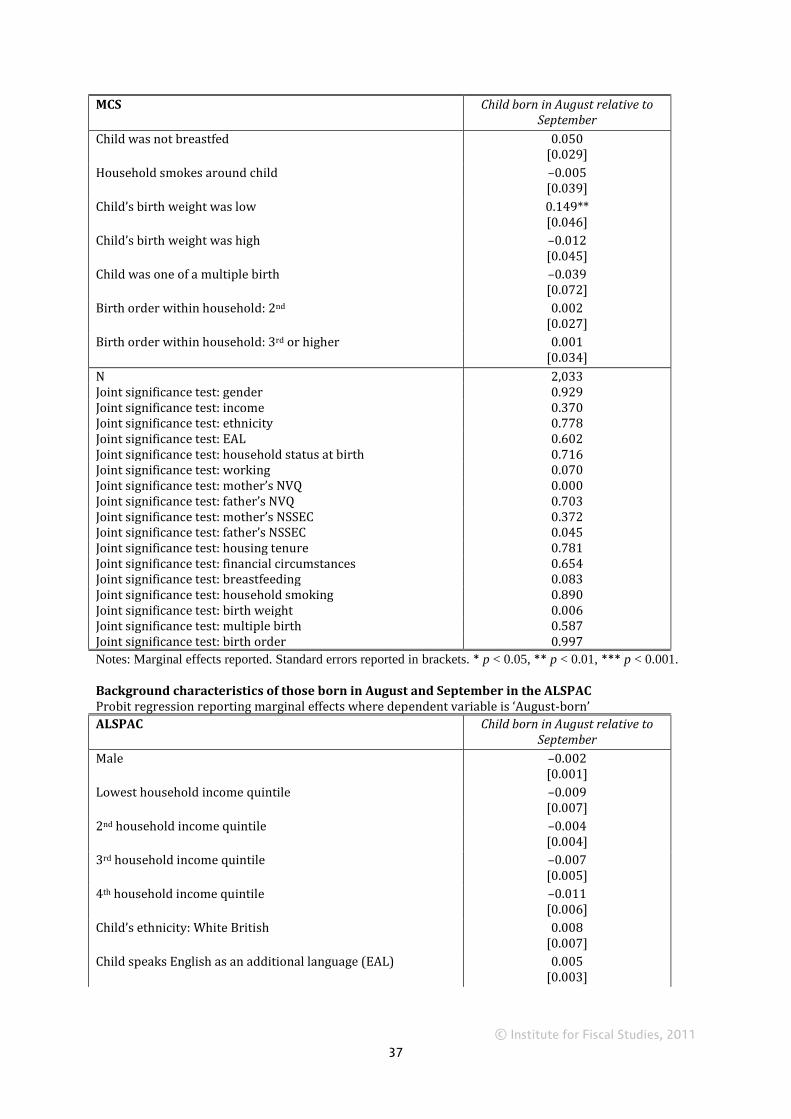
© Institute for Fiscal Studies, 2011
37
MCS Child born in August relative to September
Child was not breastfed 0.050 [0.029]
Household smokes around child –0.005 [0.039]
Child’s birth weight was low 0.149** [0.046]
Child’s birth weight was high –0.012 [0.045]
Child was one of a multiple birth –0.039 [0.072]
Birth order within household: 2nd 0.002 [0.027]
Birth order within household: 3rd or higher 0.001 [0.034]
N 2,033 Joint significance test: gender 0.929 Joint significance test: income 0.370 Joint significance test: ethnicity 0.778 Joint significance test: EAL 0.602 Joint significance test: household status at birth 0.716 Joint significance test: working 0.070 Joint significance test: mother’s NVQ 0.000 Joint significance test: father’s NVQ 0.703 Joint significance test: mother’s NSSEC 0.372 Joint significance test: father’s NSSEC 0.045 Joint significance test: housing tenure 0.781 Joint significance test: financial circumstances 0.654 Joint significance test: breastfeeding 0.083 Joint significance test: household smoking 0.890 Joint significance test: birth weight 0.006 Joint significance test: multiple birth 0.587 Joint significance test: birth order 0.997
Notes: Marginal effects reported. Standard errors reported in brackets. * p < 0.05, ** p < 0.01, *** p < 0.001.
Background characteristics of those born in August and September in the ALSPAC Probit regression reporting marginal effects where dependent variable is ‘August-born’
ALSPAC Child born in August relative to September
Male –0.002 [0.001]
Lowest household income quintile –0.009 [0.007]
2nd household income quintile –0.004 [0.004]
3rd household income quintile –0.007 [0.005]
4th household income quintile –0.011 [0.006]
Child’s ethnicity: White British 0.008 [0.007]
Child speaks English as an additional language (EAL) 0.005 [0.003]

© Institute for Fiscal Studies, 2011
38
ALSPAC Child born in August relative to September
Lone parent at 32 weeks’ gestation 0.006* [0.002]
Cohabiting at 32 weeks’ gestation 0.003 [0.002]
Household work: mother in work at age 3 –0.001 [0.002]
Household work: father in work at age 3 0.004 [0.005]
Mother’s highest educational qualification (NVQ): CSE –0.004 [0.005]
Mother’s NVQ: vocational –0.000 [0.004]
Mother’s NVQ: O level –0.002 [0.004]
Mother’s NVQ: A level –0.003 [0.004]
Father’s highest educational qualification (NVQ): CSE –0.001 [0.003]
Father’s NVQ: vocational –0.010 [0.007]
Father’s NVQ: O level 0.004 [0.002]
Father’s NVQ: A level 0.001 [0.003]
Mother’s class: ii 0.001 [0.004]
Mother’s class: iii (non-manual) 0.003 [0.004]
Mother’s class: iii (manual) 0.003 [0.003]
Mother’s class: iv –0.005 [0.008]
Mother’s class: v 0.002 [0.005]
Father’s class: ii –0.002 [0.003]
Father’s class: iii (non-manual) –0.003 [0.005]
Father’s class: iii (manual) 0.000 [0.003]
Father’s class: iv 0.003 [0.003]
Father’s class: v –0.000 [0.006]
Mother’s age at birth of child: 30–34 –0.007 [0.004]
Mother’s age at birth of child: 25–29 –0.006 [0.004]
Mother’s age at birth of child: 20–24 –0.003 [0.004]
Mother’s age at birth of child: under 20 0.001 [0.004]

© Institute for Fiscal Studies, 2011
39
ALSPAC Child born in August relative to September
Ever lived in social housing 0.000 [0.002]
Always owned/mortgaged home –0.001 [0.002]
Financial difficulties –0.004 [0.003]
Child was not breastfed 0.001 [0.002]
Household smokes around child –0.002 [0.002]
Child’s birth weight was low 0.006** [0.002]
Child’s birth weight was high 0.004 [0.003]
Child was one of a multiple birth –0.006 [0.007]
Birth order within household: 2nd 0.004* [0.002]
Birth order within household: 3rd 0.005* [0.002]
Birth order within household: 4th or higher 0.006** [0.002]
N 2,845 Joint significance test: gender 0.151 Joint significance test: income 0.086 Joint significance test: ethnicity 0.103 Joint significance test: EAL 0.192 Joint significance test: household status at birth 0.139 Joint significance test: working 0.605 Joint significance test: mother’s NVQ 0.715 Joint significance test: father’s NVQ 0.019 Joint significance test: mother’s class 0.215 Joint significance test: father’s class 0.538 Joint significance test: mother’s age at birth of child 0.133 Joint significance test: social housing 0.910 Joint significance test: own/mortgage home 0.795 Joint significance test: financial circumstances 0.095 Joint significance test: breastfeeding 0.454 Joint significance test: household smoking 0.214 Joint significance test: birth weight 0.013 Joint significance test: multiple birth 0.303 Joint significance test: birth order 0.009
Notes: Marginal effects reported. Standard errors reported in brackets. * p < 0.05, ** p < 0.01, *** p < 0.001.
Background characteristics of those born in August and September in the LSYPE Probit regression reporting marginal effects where dependent variable is ‘August-born’
LSYPE Child born in August relative to September
Male 0.002 [0.020]
Lowest household income quintile –0.026 [0.060]

© Institute for Fiscal Studies, 2011
40
LSYPE Child born in August relative to September
2nd household income quintile 0.024 [0.050]
3rd household income quintile 0.034 [0.048]
4th household income quintile 0.002 [0.045]
Young person’s ethnicity: Black Caribbean 0.072 [0.077]
Young person’s ethnicity: Black African –0.121 [0.080]
Young person’s ethnicity: Indian 0.013 [0.062]
Young person’s ethnicity: Pakistani –0.133 [0.071]
Young person’s ethnicity: Bangladeshi –0.215** [0.073]
Young person’s ethnicity: mixed –0.051 [0.065]
Young person’s ethnicity: other 0.159 [0.088]
Child speaks English as an additional language (EAL) 0.108 [0.061]
Lone parent when child was born 0.011 [0.033]
Household work: mother in part-time work at age 14 0.021 [0.032]
Household work: mother unemployed at age 14 –0.156 [0.133]
Household work: mother looking after home/family at age 14 0.027 [0.042]
Household work: mother other –0.009 [0.073]
Household work: father in part-time work at age 14 0.127 [0.077]
Household work: father unemployed at age 14 0.056 [0.100]
Household work: father looking after home/family at age 14 –0.027 [0.145]
Household work: father other 0.075 [0.066]
Mother’s highest educational qualification (NVQ): none –0.068 [0.053]
Mother’s NVQ: other 0.041 [0.102]
Mother’s NVQ: level 1 and below 0.026 [0.054]
Mother’s NVQ: GCSE grades A–C –0.016 [0.046]
Mother’s NVQ: A level or equivalent 0.050 [0.051]
Mother’s NVQ: higher education below degree level 0.015 [0.050]
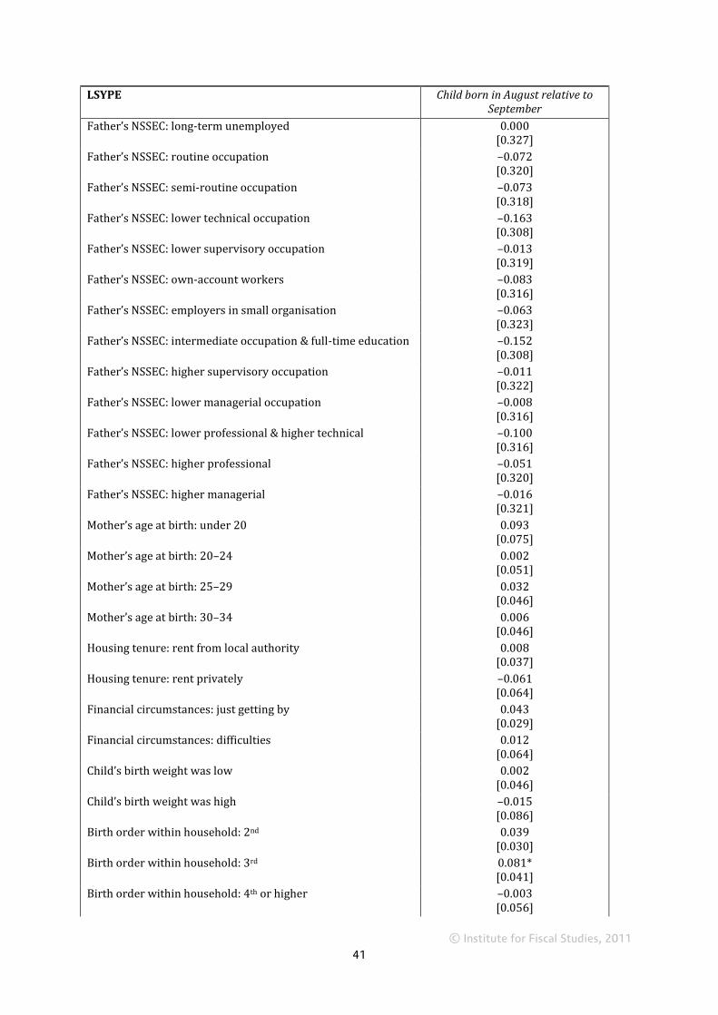
© Institute for Fiscal Studies, 2011
41
LSYPE Child born in August relative to September
Father’s NSSEC: long-term unemployed 0.000 [0.327]
Father’s NSSEC: routine occupation –0.072 [0.320]
Father’s NSSEC: semi-routine occupation –0.073 [0.318]
Father’s NSSEC: lower technical occupation –0.163 [0.308]
Father’s NSSEC: lower supervisory occupation –0.013 [0.319]
Father’s NSSEC: own-account workers –0.083 [0.316]
Father’s NSSEC: employers in small organisation –0.063 [0.323]
Father’s NSSEC: intermediate occupation & full-time education –0.152 [0.308]
Father’s NSSEC: higher supervisory occupation –0.011 [0.322]
Father’s NSSEC: lower managerial occupation –0.008 [0.316]
Father’s NSSEC: lower professional & higher technical –0.100 [0.316]
Father’s NSSEC: higher professional –0.051 [0.320]
Father’s NSSEC: higher managerial –0.016 [0.321]
Mother’s age at birth: under 20 0.093 [0.075]
Mother’s age at birth: 20–24 0.002 [0.051]
Mother’s age at birth: 25–29 0.032 [0.046]
Mother’s age at birth: 30–34 0.006 [0.046]
Housing tenure: rent from local authority 0.008 [0.037]
Housing tenure: rent privately –0.061 [0.064]
Financial circumstances: just getting by 0.043 [0.029]
Financial circumstances: difficulties 0.012 [0.064]
Child’s birth weight was low 0.002 [0.046]
Child’s birth weight was high –0.015 [0.086]
Birth order within household: 2nd 0.039 [0.030]
Birth order within household: 3rd 0.081* [0.041]
Birth order within household: 4th or higher –0.003 [0.056]

© Institute for Fiscal Studies, 2011
42
LSYPE Child born in August relative to September
N 2,047 Joint significance test: gender 0.906 Joint significance test: income 0.637 Joint significance test: ethnicity 0.018 Joint significance test: EAL 0.087 Joint significance test: household status at birth 0.737 Joint significance test: mother’s work status 0.679 Joint significance test: father’s work status 0.443 Joint significance test: mother’s NVQ 0.387 Joint significance test: father’s NSSEC 0.405 Joint significance test: mother’s age at birth of child 0.615 Joint significance test: housing tenure 0.498 Joint significance test: financial circumstances 0.303 Joint significance test: birth weight 0.191 Joint significance test: birth order 0.984
Notes: Marginal effects reported. Standard errors reported in brackets. * p < 0.05, ** p < 0.01, *** p < 0.001.

© Institute for Fiscal Studies, 2011
43
Appendix C
Variable Description MCS Child’s gender Binary variable coded to equal 1 if the child is male, and 0
otherwise; based on main parent report at Wave 1.
Household income Discrete variable for household income quintile at Wave 1, entered as a set of binary variables in the regression with ‘highest income quintile’ as the reference category. Household income is taken from a derived variable based on data reported by the main parent in Wave 1 of the survey that accounts for the composition of the family using OECD equivalence scales.
Child’s ethnicity Discrete variable reported by the main parent in Wave 1 of the survey, where categories are: White British; Black Caribbean; Black African; Indian; Pakistani; Bangladeshi; other Asian background; mixed, any background; other; missing. Entered as a set of binary variables in the regression with ‘White British’ as the reference category.
English as an additional language (EAL) Binary variable reported by the main parent in Wave 1 of the survey. Coded to equal 1 if the household speaks a language other than English in the home (including if English is also spoken), and 0 otherwise.
Household marital status at birth Discrete variable for whether the main parent was a lone parent, cohabiting or married when the child was born. Entered as a set of binary variables in the regression with ‘married’ as the reference category.
Household work status Discrete variable for whether the main and second parents were in work at Wave 1 of the survey. Categories are: both in work / on leave; main in work / on leave, partner not in work / on leave; partner in work / on leave, main not in work / on leave; both not in work / on leave. Entered as a set of binary variables in the regression with ‘both in work / on leave’ as the reference category.
Mother’s education Discrete variable for highest level of education (academic or vocational) measured at Wave 1. Categories are: none; NVQ level 1 (e.g. BTEC entry level); NVQ level 2 (e.g. GCSE A*–C); NVQ level 3 (e.g. AS/A level); NVQ 4&5 (e.g. foundation degree); NVQ 6&7 (degree and higher). Entered as a set of binary variables in the regression with ‘NVQ 6&7’ as the reference category.
Father’s education As above.
Mother’s socio-economic status Discrete variable for National Statistics Socio-Economic Classification measured at Wave 1. Categories are: high managerial/professional; low managerial/professional; intermediate; small employer & self-employed; low supervisory & technical; semi-routine; routine. Entered as a set of binary variables in the regression with ‘high managerial/professional’ as the reference category.
Father’s socio-economic status As above.

© Institute for Fiscal Studies, 2011
44
MCS continued Housing tenure Discrete variable reported by main parent at Wave 1 of the
survey. Categories are: own/mortgage/shared equity; rent privately; rent from local authority or housing association; with parents; other. Entered as a set of binary variables in the regression with ‘own/mortgage/shared equity’ as the reference category.
Financial circumstances Discrete variable from main parent’s response to the question ‘How well [is the household] managing financially these days?’ in Wave 1 of the survey. Categories are: living comfortably; doing alright; just about getting by; finding it quite difficult; finding it very difficult. Entered as a set of binary variables in the regression with ‘living comfortably’ as the reference category.
Whether child was breastfed Binary variable coded to equal 1 if the mother reports that she ever tried to breastfeed the child, and 0 otherwise; based on data provided at Wave 1.
Whether household smokes around child Binary variable coded to equal 1 if main parent reports that anyone ever smokes in the same room as the baby, and 0 otherwise; based on data provided at Wave 1.
Child’s birth weight Discrete variable created from main parent’s report of the child’s birth weight at Wave 1, coded into categories: low (less than 2.5 kg); average (2.5kg to 4.5kg); high (over 4.5kg). Entered as a set of binary variables in the regression with ‘average’ as the reference category.
Whether child was one of a multiple birth Binary variable coded to equal 1 if the child is a twin/triplet, and 0 otherwise.
Child’s birth order Discrete variable derived from the household grid. Created by counting the number of older siblings in the household at Wave 1 (including half- and step-siblings). Entered as a set of binary variables in the regression with ‘1st or only child’ as the reference category.
ALSPAC Child’s gender Binary variable coded to equal 1 if child is male, and 0
otherwise, based on health visitor records at birth.
Household income Household income is derived from postal questionnaires completed by the main carer when the child is 33 and 47 months (weekly take-home family income in five bands). Band medians were imputed with data from the Family Expenditure Survey, and an adjustment was made for families on Housing Benefit. Incomes were deflated by the RPI and equivalised using the modified OECD scale. A discrete variable for income quintiles was then created, and entered as a set of binary variables in the regression with ‘highest income quintile’ as the reference category. We thank Liz Washbrook of CMPO for providing us with her code for this variable.
Child’s ethnicity Binary variable coded to equal 1 if the child is classified as ‘White British’ in administrative data (the National Pupil Database), and 0 otherwise.
English as an additional language (EAL) Binary variable coded to equal 1 if the child is classified as having ‘English as an additional language’ in administrative data, and 0 otherwise.

© Institute for Fiscal Studies, 2011
45
ALSPAC continued Household status at 32 weeks’ gestation Discrete variable for whether the main parent was a lone
parent, cohabiting or married at 32 weeks’ gestation. Entered as a set of binary variables in the regression with ‘married’ as the reference category.
Household work status Two binary variables, one for the mother and one for the father, coded to equal 1 if they work full-time or part-time when the child is aged 3, and 0 otherwise.
Mother’s education Discrete variable for highest level of educational qualification measured at 32 weeks’ gestation. Categories are: CSE, vocational, O level, A level, degree. Entered as a set of binary variables in the regression with ‘degree’ as the reference category.
Father’s education As above.
Mother’s socio-economic status Discrete variable coding social class of the mother using the 1991 OPCS classification, based on questions at 32 weeks’ gestation about the normal job, occupation, trade or profession. Entered as a set of binary variables in the regression with ‘professional etc. occupations’ as the reference category.
Father’s socio-economic status As above.
Mother’s age at birth of child Discrete variable derived from mother’s response at 33 months. Categories are: 19 or under, 20 to 24, 25 to 29, 30 to 34, over 34. Entered as a set of binary variables in the regression with ‘over 34’ as the reference category.
Housing tenure Two binary variables created from mother’s responses to the survey from the child’s birth up to 122 months. The first binary variable is coded to equal 1 if the family has ever lived in social housing since the birth, and 0 otherwise. The second binary variable is coded to equal 1 if the family has always owned or had a mortgage for their home since the birth, and 0 otherwise.
Financial circumstances Binary variable coded to equal 1 if the partner reports a high score of financial difficulties (at least 10) at 8 months or 33 months, and 0 otherwise.
Whether child was breastfed Binary variable coded to equal 1 if the mother reports ever having breastfed the child in the 4-week, 6-month or 15-month surveys, and 0 otherwise.
Whether household smokes around child Binary variable coded to equal 1 if the mother reports that the child is in the same room as smokers at the weekend in the 6-month survey, and 0 otherwise.
Child’s birth weight Discrete variable created from main parent’s report of the child’s birth weight at 61 months, coded to categories: low (less than 2.5 kg); average (2.5kg to 4.5kg); high (over 4.5kg). Entered as a set of binary variables in the regression with ‘average’ as the reference category.
Whether child was one of a multiple birth Binary variable coded to equal 1 if the child is a twin or triplet, and 0 otherwise, based on health visitor records at birth.
Child’s birth order Derived from number of older siblings based on parent reports at 47, 61 and 81 months. Earliest information is used where possible, and only updated if this is missing for some reason. Entered as a set of binary variables in the regression with ‘1st or only child’ as the reference category.

© Institute for Fiscal Studies, 2011
46
ALSPAC continued Cohort Set of binary variables representing the academic cohort of
the child, with the middle cohort (those born between 1 September 1991 and 31 August 1992) as the reference category.
LSYPE Young person’s gender Binary variable coded to equal 1 if the child is male, and 0
otherwise, reported by the main parent in the household grid in Wave 1 of the survey.
Household income Discrete variable for household income quintile at Wave 1, entered as a set of binary variables in the regression with ‘highest income quintile’ as the reference category. Household income is taken from questions at Wave 1 of the survey. Banded income is created from parent reports. Missing values are imputed using interval regression (unless no one in the household is in work, in which case income is imputed to be zero). Household income is equivalised using OECD weights.
Young person’s ethnicity Discrete variable reported by the main parent in Wave 1 of the survey, where categories are: White; Black Caribbean; Black African; Indian; Pakistani; Bangladeshi; mixed; other; missing. Entered as a set of binary variables in the regression with ‘White’ as the reference category.
English as an additional language (EAL) Binary variable coded to equal 1 if English is an additional language in the home, and 0 otherwise. Reported by the main parent in Wave 1 of the survey.
Household status at birth Binary variable coded to equal 1 if the main parent was a lone parent when the child was born (derived from the LSYPE history file), and 0 otherwise.
Household work status Two sets of discrete variables for the mother’s and father’s work status, reported in Wave 1 of the survey. Categories are: full-time work; part-time work; unemployed; looking after home/family; other. Both are entered as a set of binary variables in the regression with ‘full-time work’ as the reference category.
Mother’s education Discrete variable for highest level of education (academic or vocational) reported in Wave 1 of the survey. Categories are: none; other; level 1 and below; GCSE grades A–C or equivalent; A level or equivalent; higher education below degree level; degree or higher. Entered as a set of binary variables in the regression with ‘degree or higher’ as the reference category.
Father’s socio-economic status Discrete variable for National Statistics Socio-Economic Classification (NSSEC) reported at Wave 1. Categories are: long-term unemployed; routine occupation; semi-routine occupation; lower technical occupation; lower supervisory occupation; own-account workers; employers in small organisations; intermediate occupation & full-time education; higher supervisory occupation; lower managerial occupation; lower professional & higher technical; higher professional; higher managerial; employers in large organisation. Entered as a set of binary variables in the regression with ‘employers in large organisation’ as the reference category.

© Institute for Fiscal Studies, 2011
47
LSYPE continued Mother’s age at birth of young person Discrete variable derived from mother’s response at Wave
1. Categories are: 19 or under; 20 to 24; 25 to 29; 30 to 34; over 34. Entered as a set of binary variables in the regression with ‘over 34’ as the reference category.
Housing tenure Discrete variable reported by the main parent at Wave 1 of the survey. Categories are: own/mortgage; rent privately; rent from local authority or housing association; other. Entered as a set of binary variables in the regression with ‘own/mortgage’ as the reference category.
Financial circumstances Discrete variable from main parent’s response to the question ‘How well [is the household] managing on income?’ at Wave 1. Categories are: managing quite well; just getting by; having difficulties. Entered as a set of binary variables in the regression with ‘managing quite well’ as the reference category.
Young person’s birth weight Discrete variable created from the main parent’s report of the child’s birth weight at Wave 1, coded to categories: low (less than 2.5 kg); average (2.5kg to 4.5kg); high (over 4.5kg). Entered as a set of binary variables in the regression with ‘average’ as the reference category.
Young person’s birth order Derived from number of older siblings reported by the young person at Wave 1. Entered as a set of binary variables in the regression with ‘1st or only child’ as the reference category.

© Institute for Fiscal Studies, 2011
48
Appendix D
Figure D.1 Proportion of young people that state they are ‘very likely’ to apply for university in the future (or have already applied or already attend university)
Note: Being ‘very likely’ to apply for university at ages 18 and 19 also includes individuals who have already applied,
and at age 19 also includes those who have already started university.
Figure D.2 Proportion of young people that state they are ‘likely’ to apply for university in the future (or have already applied or already attend university)
Note: Being ‘likely’ to apply for university at ages 18 and 19 also includes individuals who have already applied, and
at age 19 also includes those who have already started university.
0.0
0.1
0.2
0.3
0.4
0.5
0.6
0.7
0.8
14 15 16 17 18 19
Age
All August-born September-born
0.0
0.1
0.2
0.3
0.4
0.5
0.6
0.7
0.8
14 15 16 17 18 19
Age
All August-born September-born

© Institute for Fiscal Studies, 2011
49
Table D.1 Average outcomes for the sample as a whole and for those born in September
Variable All young people Young people born in September
Mean Std dev. Mean Std dev. MCS Foundation Stage Profile (FSP) total score 0 1 0.356 0.915 Key Stage 1 (KS1) average point score 0 1 0.236 1.024 British Ability Scale (BAS) total score (age 3) 0 1 0.022 1.018 BAS total score (age 5) 0.006 0.750 0.236 0.692 BAS total score (age 7) 0.006 0.790 0.174 0.801 Teacher rates below average in reading (age 7) 0.205 0.404 0.139 0.346 Teacher rates below average in writing (age 7) 0.285 0.451 0.181 0.385 Teacher rates below average in maths (age 7) 0.192 0.394 0.105 0.307 Parent states difficulty in reading (age 7) 0.280 0.449 0.266 0.442 Parent states difficulty in writing (age 7) 0.322 0.467 0.268 0.443 Parent states difficulty in maths (age 7) 0.329 0.470 0.260 0.439 Parent-reported Strengths and Difficulties Questionnaire (SDQ) (age 3)
0 1 –0.013 0.953
Parent-reported SDQ (age 5) 0 1 0.063 0.988 Parent-reported SDQ (age 7) 0 1 0.056 1.003 Teacher-reported SDQ (age 7) 0 1 0.153 0.965 Parent paid for additional lessons (age 7) 0.053 0.224 0.048 0.215 Home learning environment (age 3) 0 1 –0.035 0.966 Home learning environment (age 5) 0 1 –0.009 1.009 Home learning environment (age 7) 0 1 –0.036 1.003 Child doesn’t like school (age 7) 0.162 0.369 0.139 0.346 Always unhappy at school (age 7) 0.071 0.257 0.048 0.214 Parent reports child is bullied at least several times (age 7)
0.072 0.259 0.071 0.257
Child reports always bullied (age 7) 0.094 0.292 0.065 0.246 Child reports always/sometimes bullied (age 7) 0.495 0.500 0.469 0.499 ALSPAC KS1 capped points score 0 1 0.262 0.936 KS2 average points score 0 1 0.185 0.948 KS4 capped and equivalents total points score 0 1 0.131 0.964 WISC (IQ) (age 8) 0 1 –0.057 0.981 WOLD comprehension (age 8) 0 1 0.014 1.007 NARA comprehension (age 9) 0 1 0.043 1.012 Plans to continue in post-16 full-time education (age 14)
0.882 0.323 0.882 0.323
Teacher reports child is ‘very ready’ for secondary school
0.557 0.497 0.630 0.483
Parent-reported SDQ (age 7) 0 1 0.034 0.989 Parent-reported SDQ (age 9) 0 1 0.022 1.013 Parent-reported SDQ (age 11) 0 1 0.055 0.984 Parent-reported SDQ (age 13) 0 1 0.057 0.974 Teacher-reported SDQ (age 8) 0 1 0.055 0.994 Teacher-reported SDQ (age 11) 0 1 0.070 0.984 Home learning environment (age 3) 0 1 0.029 1.031 Child doesn’t like school (age 8) 0.192 0.394 0.194 0.396 Scholastic competence (age 8) 0 1 0.140 0.962 Global self-worth (age 8) 0 1 0.044 0.973 Locus of control (age 8) 0 1 0.024 0.975 Victim of bullying (age 8) 0.282 0.450 0.280 0.449 Victim of bullying (age 10) 0.200 0.400 0.213 0.410 Smokes at least 1–6 cigarettes per week (age 14) 0.034 0.182 0.030 0.170 Smokes at least sometimes (age 14) 0.061 0.239 0.054 0.227 Has ever tried cannabis (age 14) 0.086 0.280 0.065 0.248

© Institute for Fiscal Studies, 2011
50
Variable All young people Young people born in September
Mean Std dev. Mean Std dev. LSYPE KS2 average points score 0 1 0.197 0.971 KS3 average points score 0 1 0.154 0.981 KS4 capped and equivalents total points score 0 1 0.094 0.968 Achieved 5 or more GCSE/GNVQs at grades A*–C 0.580 0.494 0.627 0.484 Plans to continue in post-16 full-time education (age 14)
0.839 0.368 0.864 0.342
Very likely to apply to university (age 14) 0.338 0.473 0.371 0.483 Very likely to apply to university (age 15) 0.319 0.466 0.332 0.471 Very likely to apply to university (age 16) 0.354 0.478 0.373 0.484 Very likely to apply to university (age 17) 0.384 0.486 0.402 0.491 Very likely to apply to university OR has already applied (age 18)
0.456 0.498 0.463 0.499
Very likely to apply to university OR has already applied OR is at university (age 19)
0.530 0.499 0.543 0.499
Likely to apply to university (age 14) 0.687 0.464 0.710 0.454 Likely to apply to university (age 15) 0.630 0.483 0.660 0.474 Likely to apply to university (age 16) 0.606 0.489 0.644 0.479 Likely to apply to university (age 17) 0.563 0.496 0.599 0.490 Likely to apply to university OR has already applied (age 18)
0.566 0.496 0.580 0.494
Likely to apply to university OR has already applied OR is at university (age 19)
0.606 0.489 0.608 0.489
Full-time education (age 17) 0.724 0.447 0.730 0.444 Academic course post-16 (age 17) 0.678 0.467 0.692 0.462 Vocational course post-16 (age 17) 0.359 0.480 0.347 0.476 University participation (age 19) 0.287 0.452 0.282 0.450 Russell Group university participation (age 19) 0.074 0.262 0.084 0.278 Parent paid for additional academic lessons (age 14)
0.069 0.253 0.072 0.259
Parent paid for additional academic lessons (age 15)
0.106 0.308 0.119 0.324
Parent paid for additional academic lessons (age 16)
0.062 0.241 0.065 0.246
Ability beliefs (age 14) 0 1 0.096 0.953 Usefulness of school (age 14) 0 1 0.050 0.969 Value of school (age 17) 0 1 0.005 1.016 Young person doesn’t like school (age 14) 0.126 0.332 0.115 0.319 Young person is unhappy at school (age 14) 0.142 0.349 0.122 0.327 High score on bullying scale (age 14) 0.294 0.456 0.280 0.449 High score on bullying scale (age 15) 0.272 0.445 0.291 0.455 High score on bullying scale (age 16) 0.288 0.453 0.270 0.444 High score on bullying scale (age 17) 0.269 0.443 0.278 0.448 Smokes at least sometimes (age 14) 0.078 0.268 0.105 0.306 Smokes at least sometimes (age 16) 0.215 0.411 0.247 0.431 Drunk alcohol at least once a month for the past 12 months (age 14)
0.245 0.430 0.277 0.448
Drunk alcohol at least once a month for the past 12 months (age 15)
0.386 0.487 0.422 0.494
Drunk alcohol at least once a month for the past 12 months (age 16)
0.489 0.500 0.518 0.500
Drunk alcohol at least once a month for the past 12 months (age 17)
0.676 0.468 0.703 0.457
Drunk alcohol at least once a month for the past 12 months (age 18)
0.855 0.353 0.865 0.342
Ever tried cannabis (age 14) 0.088 0.283 0.112 0.315

© Institute for Fiscal Studies, 2011
51
Variable All young people Young people born in September
Mean Std dev. Mean Std dev. LSYPE continued Ever tried cannabis (age 15) 0.097 0.296 0.130 0.336 Ever tried cannabis (age 16) 0.211 0.408 0.252 0.434 Ever tried cannabis (age 17) 0.281 0.450 0.322 0.468 Ever tried cannabis (age 18) 0.389 0.488 0.422 0.494 Ever plays truant (age 14) 0.157 0.364 0.155 0.362

© Institute for Fiscal Studies, 2011
52
References
Bedard, K. and E. Dhuey (2006), The persistence of early childhood maturity: international evidence of
long-run age effects, Quarterly Journal of Economics, 121, 1437–72.
Bedard, K. and E. Dhuey (2009), School entry policies and skill accumulation across directly and indirectly
affected men, University of Toronto, mimeo.
Black, S., Devereux, P. and Salvanes, K. (2008), Too young to leave the nest? The effects of school starting
age, NBER Working Paper 13969.
Blundell, R., L. Dearden and B. Sianesi (2005), Evaluating the impact of education on earnings: models,
methods and results from the NCDS, Journal of the Royal Statistical Society, Series A, 168, 473–512.
Buckles, K. and D. Hungerman (2008), Season of birth and later outcomes: old questions, new answers,
NBER Working Paper 14573.
Carneiro, P., C. Crawford and A. Goodman (2007), The impact of early cognitive and non-cognitive skills
on later outcomes, CEE Discussion Paper 92.
Cebi, M. (2007), Locus of control and human capital investment revisited, Journal of Human Resources, 42,
919–32.
Chevalier, A. and G. Conlon (2003), Does it pay to attend a prestigious university?, IZA Discussion Paper
848.
Chowdry, H., C. Crawford and A. Goodman (2009), Drivers and Barriers to Educational Success: Evidence
from the Longitudinal Survey of Young People in England, DCSF Research Report DCSF-RR102.
Crawford, C., L. Dearden and C. Meghir (2007), When You Are Born Matters: The Impact of Date of Birth on
Child Cognitive Outcomes in England, Centre for the Economics of Education Report to the Department for
Children, Schools and Families (http://www.ifs.org.uk/publications/4073).
Datar, A. (2006), Does delaying kindergarten entrance give children a head start?, Economics of Education
Review, 25, 43–62.
Dearden, L. (1999), The effects of families and ability on men’s education and earnings in Britain, Labour
Economics, 6, 551–67.
Dearden, L., S. McIntosh, M. Myck and A. Vignoles (2002), The returns to academic and vocational
qualifications in Britain, Bulletin of Economic Research, 54, 249–74.
Department for Education (2010), Month of Birth and Education, DfE Research Report 17.
Dhuey, E. and S. Lipscomb (2008), What makes a leader? Relative age and high school leadership,
Economics of Education Review, 27, 173–83.
Dhuey, E. and S. Lipscomb (2010), Disabled or young? Relative age and special education diagnoses in
schools, Economics of Education Review, 29, 857–72.
Dickert-Conlin, S. and T. Elder (2010), Suburban legend: school cutoff dates and the timing of births,
Economics of Education Review, 29, 826–41.
Dobkin, C. and F. Ferreira (2010), Do school entry laws affect educational attainment and labor market
outcomes?, Economics of Education Review, 29, 40–54.
Duckworth, A., C. Peterson, M. Matthews and D. Kelly (2007), Grit: perseverance and passion for long-
term goals, Journal of Personality & Social Psychology, 92, 1087–101.
Duncan, R. and G. Dunifon (1998), Long-run effects of motivation on labor market success, Social
Psychology Quarterly, 61, 33–48.

© Institute for Fiscal Studies, 2011
53
Elder, T. and D. Lubotsky (2009), Kindergarten entrance age and children’s achievement: impacts of state
policies, family background and peers, Journal of Human Resources, 44, 641–83.
Feinstein, L. (2002a), Quantitative Estimates of the Social Benefits of Learning, 1: Crime, Wider Benefits of
Learning Research Report 5, Institute of Education, London.
Feinstein, L. (2002b), Quantitative Estimates of the Social Benefits of Learning, 2: Health (Depression and
Obesity), Wider Benefits of Learning Research Report 6, Institute of Education, London.
Fredriksson, P. and B. Ockert (2005), Is early learning really more productive? The effect of school
starting age on school and labour market performance, IZA Discussion Paper 1659.
Gans, J. and A. Leigh (2009), Born on the first of July: an (un)natural experiment in birth timing, Journal of
Public Economics, 93, 246–63.
Goodman, A. and P. Gregg (2010), Poorer Children’s Educational Attainment: How Important Are Attitudes
and Behaviours?, Report to the Joseph Rowntree Foundation.
Goodman, R., J. Gledhill and T. Ford (2003), Child psychiatric disorder and relative age within school year:
cross sectional survey of large population sample, British Medical Journal, 327, 1–4.
Hammond, C. and L. Feinstein (2006), Are Those who Flourished at School Healthier Adults? What Role for
Adult Education?, Wider Benefits of Learning Research Report 17, Institute of Education, London.
Harter, S. (1985), Manual for the self-perception profile for children, University of Denver, mimeo.
Kawaguchi, D. (2011), Actual age at school entry, educational outcomes, and earnings, Journal of the
Japanese and International Economies, 25(2), 64–80.
Mühlenweg, A. (2010), Young and innocent: international evidence on age effects within grades on
victimization in elementary school, Economics Letters, 109, 157–60.
Mühlenweg, A., D. Blomeyer and M. Laucht (2011), Effects of age at school entry on the development of
non-cognitive skills: evidence from psychometric data, ZEW Discussion Paper 11-017.
Neale, M. (1997), Neale Analysis of Reading Ability – Revised, NFER-Nelson, Windsor.
Nowicki, S. and B. Strickland (1973), A locus of control scale for children, Journal of Consulting and Clinical
Psychology, 40, 148–54.
Osborne Groves, M. (2005), How important is your personality? Labor market returns to personality for
women in the US and UK, Journal of Economic Psychology, 26, 827–41.
Puhani, P. and A. Weber (2007), Does the early bird catch the worm? Instrumental variable estimates of
early educational effects of age of school entry in Germany, Empirical Economics, 32, 359–86.
Rust, J. (1996), The Manual of the Wechsler Objective Language Dimensions, The Psychological
Corporation, London.
Sharp, C. (1995), What’s age got to do with it? A study of patterns of school entry and the impact of season
of birth on school attainment, Education Research, 37, 251–65.
Smith, J. (2009), Can regression discontinuity help answer an age-old question in education? The effect of
age on elementary and secondary school achievement, The B.E. Journal of Economic Analysis & Policy, 9,
issue 1 (Topics), article 48.
Solli, I. (2011), Left behind by birth month, University of Stavanger, mimeo.
Wechsler, D., S. Golombok and J. Rust (1992), Wechsler Intelligence Scale for Children – Third Edition, UK
Manual, The Psychological Corporation, Sidcup, UK.