DOCUMENT RESUME

ED 329 420 RC 018 039

AUTHOR Cautley, Eleanor K.TITLE Rural-Urban Differences in Employment, Household

Composition, and Poverty Status among SingleMothers.

SPONS AGENCY Economic Research Service (DOA), Washington, D.C.PUB DATE 89

NOTE 95p.; M.S. Thesis, University ofWisconsin-Madison.

PUB TYPE Dissertations/Theses - Masters Theses (042)

EDRS PRICE MF01/PC04 Plus Postage.DESCRIPTORS Census Figures; Dependents; *Employment Level; Family

Characteristics; Family Income; *Family Structure;Fatherless Family; Heads of Households; *Mothers;*One Parent Family; *Poverty; Rural Family; *RuralUrban Differences

ABSTRACTUsing 1980 Census data, this study examined household

composition and labor force participation for single motherhouseholds in urban and rural areas. The study used Census data on arepresentative random sample of 5,712 female headea familyhouseholds. Variables studied were rura7.-urban status, householdcomposition, labor force participation, and poverty status. The studycontrolled for race, education, marital status, and age. Adescriptive analysis of the data used crosstabulation, group means,and proportions in poverty, while multivariate analysis methods weremultiple classification analysis and least squares multipleregression analysis. Significant findings were: (1) single motherhouseholds in small town and rural areas experience povert/ levels ashigh or higher than those in central city and suburban areas; (2)

extra adults living in the household and earnings from employment ofthese extra adults are both associated with decreased family povertylevels; and (3) employment of the single mother is the most importantvariable associated with decreased family poverty. Policyrecommendations include wage equity policies across geographic areas,increased levels of support from absent fathers, and assistance withcosts of day care and health care for single parents. This papercontains 9 data tables and 54 references. (KS)

***********************************************************************

Reproductions supplied by EDRS are the best that can be madefrom the original document.

*******************************************************t***************

RURAL-URBAN DIFFERENCES IN EMPLOYMENT, HOUSEHOLD COMPOSITION,

AND POVERTY STATUS AMONG SINGLE MOTHERS

by

ELEANOR K. CAUTLEY

A thesis submitted in partial fulfillment of the

requirements for the degree of

MASTER OF SCIENCE

at the

UNIVERSITY OF WISCONSIN-MADISON

1989

BEST COPY AVAILABLE

"PERMISSION TO REPRODUCE THISMATERIAL HAS BEEN GRANTED BY

Ete4bior (12y414,01

TO THE EDUCATIONAL RESOURCESINFORMATION CENTER (ERIC)."

U.S. DEPARTMENT OF EDUCATION°flirt. of Educational Research and improvement

EDUCATIONAL RESOURCES INFORMATIONCENTER (ERIC)

document has been repronoced ssreceived 1mm the person or organizstron

originating it1 Minor changes have been made lo improve

reproduction Quality

Points ol view or opinions staled in thisdocu

ment do nol necessarily represent official

OE RI position or POliCy

APPROVED

Doris P. Slesinger, Ph.D7Professor of Sociologyand Rural Sociology

Date

TABLE OF CONTENTS

LIST OF TABLES

ACKNOWLEDGEMENTS iii

ABSTRACT

INTRODUCTION 1

PREVIOUS RESEARCH 4

Rural-Urban Comparisons 5

Household Composition 7

Labor Force Participation 11

THEORY AND HYPOTHESESHypotheses

17

21

METHODOLOGY 24

Sample 24

Definitions 25

Variables 25

Limitations on Census Data 30

Statlstical Methods 31

DATA ANALYSIS 34

Characteristics of Single Mothers and Their Households 34

Poverty Status and Characteristics of Single MotherHouseholds 44

Multivariate Analysis 54

CONCLUSIONS 69

Summary 69

Discussion 72

FOOTNOTES 76

APPENDIX A. Sampling, Weighting, and Data Extract 77

APPENDIX B. Nonrelatives and Poverty Status 79

REFERENCES 81

ii

LIST OF TABLES

Table 1. Characteristics of Single Mothers by Urban-RuralResidence, 1980 35

Table 2. Composition of Single Mother Households byUrban-Rural Residence, 1980 38

Table 3. Poverty Status of Single Mother Families byUrban-Rural Residence, 1979 43

Table 4. Proportion Poor by Urban-Rural Residence forCharacteristics of Single Mother Households, 1979 45

Tablr J. Multiple Classification Analysis of ProportionPoor for Selected Demographic Characteristics ofSingle Mother Households

Table 6. Multiple Classification Analysis of Effect ofAdditional Adults in Single Mother Households onProportion Poor in Urban and Rural Areas

55

57

Table 7A. Multiple Classification Analysis of Effects ofAdults Earning Income in Single Mother Households onProportion Poor in Urban and Rural Areas 59

Table 78. Multiple Classification Analysis of Effect ofLabor Force Variables on Poverty in Single MotherHouseholds in Urban and Rural Areas 61

Table 8. Multiple Regression Analysis of the Effect ofAdults and Employed Persons on Income-Needs Ratio forSingle Mother Households in Urban and Rural Areas 66

iii

ACKNOWLEDGEMENTS

This thesis was completed with the encouragement and support of

many people. The Department of Rural Sociology has been my

intellectual home for 15 years, and the environment that the

Department provided was especially supportive in my completion of

this work. Many staff and students played a role in creating this

atmosphere. I would like especially to thank Pilar Parra, Josephine

Beoku-Betts, Francine Horton, and Mochammad Sjachrani for their

friendship and advice. Most importantly, I want to acknowledge the

special support given me by my academic advisor and long-time

employer, Professor Doris P. Slesinger. This thesis would not have

been possible without her patience, advice, and encouragement. I

have benefitted from her teaching in more ways than I can list.

Doris' commitment to sociology as a path to bettering the world for

the disadvantaged has helped convince me that this work is

worthwhile. Thank you, Doris.

The data set used for this analysis is the product of the labor

of several people. The 1980 Census data tapes were graciously

provided by Professor Glenn V. Fuguitt and Research Assistant Robert

Jenkins. Additional variables were created by Cheryl Knobeloch;

Professor James Sweet generously provided access to these

6

iv

variables. Bruce Christenson designed the stratified sampling

method and assisted with many details of the data sampling and

weighting process. I especially wish to thank him for the

conceptual design of the weighting procedure.

Some of the financial support for this work came from a

Cooperative Agreement with the Economic Research Service, United

States Department of Agriculture, and I particularly want to thank

Dr. Peggy Ross. Computing hardware and software used for this

research was provided by the Center for Demography and Ecology,

NCCHD grant HD-05876.

I would like to thank Professor Sara McLanahan and Professor

James Sweet for serving on my master's examining committee. Their

insightful comments have helped improve this work.

Karen Morgan's very able assistance in word processing has eased

the way for me many times, and I thank her for her special

assistance on this project. I also appreciate the encouragement of

my new colleagues at the Center for Health Statistics. Last and

certainly not least, I want to thank my family and friends for their

unfailing support during this project. I especially want to

acknowledge the encouragement I received from J. Michael Blohm; his

friendship has been a great source of comfort during all the trials

and tribulations of completing this thesis.

1

ABSTRACT

Single mother households experience very high levels of poverty

as well as high levels of labor force participation. This research

examines household composition and labor force participation for

single mother households in urban and rural areas. A sample of 1980

U.S. Census data is used which classifies residence into central

city, suburb, small town and rural areas. Overall, single mother

households in small town and rural areas experience poverty levels

as high or higher than those in central city and suburban areas,

when controlling for characteristics of the single mother.

Using family poverty status as the dependent variable, this

thesis confirms the hypothesis th..It extra adults living in the

single mother's household, and earnings from employment of these

extra adults, are both associated with decreased family poverty

levels. These relationships remain strong when controlling for

race, education, marital status and age of the single mother.

Employment of the single mother stands out clearly as the single

most important variable associated with decreased family poverty.

Analysis of poverty across the rural-urban continuum provides

mixed evidence for employment. Among employed single mothers,

vi

highest poverty levels occur in smnll towns, followed by central

cities, rural areas and suburbs. Effects of unobserved variables

such as pay scales appear to influence poverty levels among employed

mothers. Policy recommendations include wage equity policies across

geographic areas, increased levels of support from absent fathers,

and assistance with costs of day care and health care for single

parents.

RURAL-URBAN DIFFERENCES IN EMPLOYMENT, HOUSEHOLD COMPOSITION,

AND POVERTY STATUS AMONG SINGLE MOTHERS

Single mothers have been the focus of a great deal of research

in recent years. The dramatic growth in this population has been

well documented. The number of single mother families with minor

children increased from 2.9 million in 1970 to 5 million in 1980,

and continues to increase at a steady rate. As a proportion of all

families with minor children, single mother families have increased

dramatically: from 10.2 percent in 1970 to 16.7 percent in 1980

(U.S. Bureau of the Census, 1971 and 1981). The very high poverty

rates among single mother families have also been investigated. In

1979, for example, 40 percent of single mother families were poor,

while only 8 percent of all other families with minor children were

poor (U.S. Bureau of the Census, 1983, Table 108). The term

"feminization of poverty" served to focus even more attention on the

problems of single mothers and their children. Of all poor families

with children in 1979, 53 percent were single mother families. This

has led to concern for the long-term consequences of poverty for so

many mothers and children as well as concerns with implications for

the welfare system.

2

Often overlooked in this crisis of the feminization of poverty

is the fact that a large proportion of single mothers are employed.

Increases in the labor force participation rates of all women have

been well documented: 43 percent of all women were in the labor

force in 1970; this increased to 52 percent in 1980 and to 54

percent in 1985. (All data in this paragraph are from Taeuber and

Valdisera, 1986 except where noted.) Employment rates of mothers

are increasing at an even faster pace: while 40 percent of married

mothers with children under 18 were in the labor force in 1970, this

jumped to 54 percent in 1980 and to over 60 percent in 1985. The

high labor force participation rates of single mothers in

particular, however, are rarely noted. In 1970, 59 percent of

single mothers with minor children were in the labor force, and this

increased to 68 percent in 1980 (U.S. Bureau of the Census, 1984,

Table 274). Despite these high rates of employment, single mothers

and their children are one of the poorest groups in the United

States today.

This research looks more closely at the characteristics of

single mother households, and at the relationship between employment

and poverty among these households. There are several important

facets to this relationship, which will be examined in detail here.

These facets include household composition and employment status of

household members. Other factors, including characteristics of the

mother, also affect poverty status. Area of residence is another

facet: characteristics of rural and urban women differ, and urban

3

women have different options for employment than do rural women.

This study will describe differences between single mother

households in rural and urban areas, and examine the relationship

between employment and poverty.

4

PREVIOUS RESEARCH

Poverty status is measured by comparing family income to a

federal poverty threshold specific to family size. Families with

incomes above the threshold are not poor; below it they are poor.

Thus it is an absolute index of family income adequacy; it is not a

relative index which could address issues of income distribution and

inequality. The federal poverty thresholds have been in use since

1960, with some modifications over the years. The thresholds are

inflated yearly with the Consumer Price Index. A very large body of

literature examines causes and correlates of poverty in the United

States. There is strong agreement among researchers that being poor

is clearly related to one's race, educational attainment, gender,

and participation in the labor force. It is also generally

understood that poverty is not solely attributable to individual

characteristics; social class and societal institutions are also a

part of the causal model.

This section reviews the literature on women and poverty status,

with special attention to: 1) rural-urban comparisons; 2) household

composition; and 3) labor force participation. Some of the research

concerns all women, some concerns only married women or married

mothers, and some concerns just single mothers.

5

Rural-Urban Comparisons

There are two different wayc of defining rural and urban

residence in the United States. The more commonly used definition

distinguishes between metropolitan and nonmetropolitan residence.

Each county in the United States is classified as either metro or

nonmetro; metro counties generally have a city of 50,000 or more

surrounded by additional urbanized area, or they are adjacent

counties economically tied to the central city county. Nonmetro

counties make up the balance of the country. At the time of the

1980 census, almost 75 percent of the U.S. population lived in

metropolitan areas. The other definition of rural and urban

residence uses a smaller level of geography, and divides the nation

into Urbanized Areas and outside of Urbanized Areas. Urbanized

areas generally include a central city of 50,000 or more inhabitants

plus the closely settled suburbs. The remaining area includes two

additional groupings: rural areas, which are towns smaller than

2,500 and the open countryside; and ether urban areas, consisting of

towns of 2,500 or more. In 1980, 61.4 percent of the population

lived in urbanized areas.

Relatively little research has used rural-urban, rather than

metro-nonmetro, comparisons of populations. Hanson (1982), defining

rural as communities with less than 2,500 persons, found significant

differences between women from rural and urban backgrounds in terms

of their occupational status and earnings. Rural women who migrated

6

to urban areas Improved their occupational statuti, but never caught

up with women who came from urban backgrounds. Hanson concludes

that her findings support both the theory of segmented labor

markets, and the importance of the interacaon between human capital

variables and structural differences in urban and rural labor

markets. Cautley and Slesinger (1988), using the Urbanized Area

concept, find rural single mothers earn lower wages than urban

mothers, with the difference being primarily due to lower pay scales

in rural areas, and not to differing occupational structures. Much

of the literature on rural women concerns only farm women (Haney,

198, aaney states the need for much more research to be done.

A alAch larger body of research compares metropolitan and

nonmetropolitan populations (Hoppe, 1988; McGranahan et al., 1986;

McLaughlin and Sachs, 1988; O'Hare, 1988; Weinberg, 1987). While

Wilson et al. (1987) have argued that poverty is increasingly a

metropolitan problem, due to the size of the poor population in

central cities, the poverty rate in nonmetropolitan areas has become

perhaps more entrenched. Deavers, Hoppe and Ross (1986) note that

not only is the nonmetropolitan poverty rate consistently higher

than the metropolitan rate, but there were numerically more poor

persons in nonmetropolitan counties than in central cities in 1983.

Ghelfi (1986) points out that 93 percent of black nonmetropolitan

families live in the South, where they experience poverty rates much

higher than the national average, and indeed higher than blacks in

any other region, metropolitan or nonmetropolitan. Ross and

7

Morrissey (1986) found that persistent poverty, defined as being

poor during 3 or more years in a 5 year period, was more prevalent

in nonmetropolitan than in metropolitan areas. Using data from the

Panel Study of Income Dynamics (PSID) for 1978-1982, Ross and

Morrissey find that 8.4 percent of nonmetropolitan residents were

persistently poor, as contrasted with 5.1 percent of metropolitan

residents.

Household Composition

Single mother families have been an increasing proportion of all

families with minor children since 1950. Research on the causes for

this growth of single mother families from 1970 to 1980 reveals

distinct differences by race: for white single mothers, marital

disruption is the primary component, followed by population growth.

For blacks, population growth, followed by increases in both never

married women and marital disruption, are the major components

(Wojtkiewicz, McLanahan and Garfinkel, 1987). Research on trends in

divorce and family disruption indicate that the pattern of

increasing single mother families is not likely to change in the

foreseeable future. Using 1985 data, Castro and Bumpass (1987)

conclude that trends in separation and divorce are not decreasing,

as some have described, but will probably remain at relatively high

levels. Bumpass calculates that "abaut two-fifths of children born

to married mothers will experience the disruption of that marriage"

before reaching adulthood (1984:71).

I;

8

The research on single mothers and poverty is recent and

extensive (Bane, 1986; Duncan and Rodgers, 1987; Garfinkel and

McLanahan, 1985, 1986; Goldberg and Kremen, 1987; Kniesner, McElroy

and Wilcox, 1986; McLanahan, Garfinkel and Watson, 1986). The

increase of single mothers with children as a proportion of the poor

population has been well documented: 26.7 percent of the poor lived

in single mother households in 1970 and 33.2 percent in 1980. This

increasing proportion is due to two factors: the growth of the

single mother family population, and declining poverty rates among

other groups, particularly the elderly (Garfinkel and McLanahan,

1985). Although the actual poverty rates experienced by single

mother families.have declined slightly from 1960 to 1980, their

poverty rates are consistently much higher than those of two parent

families, and this has been true since at least 1967 (Garfinkel and

McLanahan, 1986). In their definitive work on the prevalence and

welfare dependence of sin&le mothers, Garfinkel and McLanahan (1986)

discuss three major reasons for high poverty levels among single

mother families: low wages and limited earning power for many

mothers who head households; low or zero amounts of child support

paid by absent fathers; very low levels of support provided by most

public assistance programs.

A comparison of single mother families and married couple

families clarifies the reasons for higher poverty among single

mothers. Although the average earnings of single mothers are

somewhat greater than those of married mothers, they are extremely

9

low in comparison to earnings of married fathers (Bane and Ellwood,

1989). The child support paid by absent fathers is inconsequentiai

when compared to average earnings of married fathers. Bane and

Ellwood (1989) also present data to demonntrite the work

disincentive effects of welfare program benefits. The single mother

who works full time at a wage of $6 per hour will have a maximum of

$3000 more disposable income compared to the full time welfare

recipient, and she will not have access to Medicaid health care

benefits. Only the mothers who have significant work experience or

higher levels of education are likely to benefit from working

instead of receiving welfare.

Bane and Ellwood (1986) present a classification of events which

are associated with tho beginning and ending of a "spell" of

poverty. For single mothers, the change to a female-headed family

from another family type accounts for over half of all beginnings;

declining earnings of household members accounts for another

one-cluarter of transitions into poverty. One-third of poverty

periods !or single mothers end when the mother's income increases.

Another one-fourth end with marriage of the mother, almost one-fifth

end with an increase in unearned income, and another one-fifth end

when earnings of other household members increased. Thus, changes

in household composition are most important for initiating poverty

spells, while increases in household income are most important in

ending them.

Bane (1986) challenges the assumption that changes in family

10

structure cause poverty. Using PSID data on transitions of

individuals into poverty (lasting one year or more), she tabulates

poverty spells that began before, simultanet,a to, and after a

transition to a female headed household. Periods of poverty

beginning simultaneously with a family structure transition are

"event-driven", while transitions occurring to already-poor families

are merely "reshuffling" existing poverty into new households.

There are striking diffqrences between whites and blacks: for

whites, 14 percent of poverty spells began before the household

transition, 49 percent were simultaneous, and 37 percent began after

transition; for blacks, 33 percent were tefore, 22 percent

simultaneous, and 45 percent after. Bane concludes that "(mlost

poverty, even that of female-headed families, occurs because of

income or job changes." (1986:231).

The length of time that a family may spend in poverty varies

widely, especially by race. Blacks are likely to have a period of

poverty averaging 6.5 years, or almost twice the 3.4 years for

whites (Bane and Ellwood, 1986). Thus, black single mothers will be

disproportionately represented in a cross-sectional sample of poor

single mother families.

Garfinkel and McLanahan (1986:Tables 1-2) show a strong

relationship of marital status and race with source of income for

single mother families. For example, the proportion of divorced

mothers with earned income is much higher than for any other marital

status. Not surprisingly, widows are much wire likely to have

11

Social Security income than are other women. In general, the

proportions of black mothers receiving each type of income are lower

than the proportions of white women. The exceptions occur in the

public assistance and food stamp categories; with black mothers

averaging more income from these sources than whites.

Overall, widows with children are much less likely to be poor

than are other single mothers, mainly due to higher benefit levels

paid by Social Security as compared to other income transfer

programs. Among white single mothers, widows have the highest

income while, among blacks, divorced mothers' income is highest on

average.

Labor Force Participation

The literature on women in the labor force is quite extensive,

but relatively little focuses on single mothers as an analytic

entity. Until recently, much of the analysis focused on labor force

activity of wives (Sweet, 1973; Smith-Lovin and Tickamyer, 1981).

Traditionally, wives left the labor force, often for an extended

period of time, after the birth of a child. Smith-Lovin and

Tickamyer (1981) found two very different patterns for wives --

"workers" were those who tended to remain continuously in the labor

force during childbearing years while "nonworkers" dropped out of

the labor force at time of first birth and rarely returned. Sweet

(1973) found that wives' employment rates increased as age of

youngest child increased. Labor force participation rates of wives

f'^

12

have increased steadily since 1950, with the larg3st proportional

increases occurring among mothers of young children. In 1950, 12

percent of wives with a child under six years were employed; in

1980, 45 percent were employed (Taeuber and Valdisera, 1986).

Recent research has focused on this increasing labor force

participation of mothers, including those with very young children

(O'Connell and Bloom, 1987). The increase in working mothers

prompted interest in child care arrangements used by working mothers

(Presser and Baldwin, 1980; O'Connell and Bloom, 1987) and the

variations in shifts used by working parents to accommodate child

care needs (Presser, 1986).

Although men are more likely than women to be in the labor

force, and more likely to be full time year round workers, the gap

in proportion working between men and women is narrowing. kmong

employed women in 1984, 48 percent were full time year-round workers

(Taeuber and Valdisera, 1986). The overall increasing labor force

participation of women has been due primarily to increases in full

time work (i.e., 35 hours or more per week). Currently, two-thirds

of all employed women are full time workers (Taeuber and Valdisera,

1986).

In general, black women have higher labor force participation

rates than white women. Historically, nonwhite women's labor force

rates have been highot. than white rates, at least since 1890; the

nonwhite and white) rates have slowly converged over the decades

(Sweet, 1973; Bitnchi and Spain, 1986). More recently, the

13

difference between black and white women has narrowed considerably:

in 1985, 56 percent of black women age 16 and over were in the labor

force, compared to 54 percent of similar white women (Taeuber and

Valdisera, 1986). Among women under age 25, white women have had,

and continue to have, higher labor force participation rates than

black women.

One of the most striking results of research on female labor

force participation is the clear differentiation between jobs

available to women and to men (Waite, 1981; Bergmann, 1986). This

aex segregation of occupations is due to a combination of factors,

including availability of a female labor supply that is educated and

skilled, willing to work for lower wages than men, and seen as

possessing attributes desirable to employers (Oppenheimer, 1970).

There is some evidence of slowly declining occupational sex

segregation over the decades. Using 1900, 1950, and 1980 Census

data with consistent occupation coding, Jacobs (1987) finds that

both differences between sexes in occupations and the degree of

concentration of women in occupations, as measured by an index of

dissimilarity, have declined since 1900. Thus, women have become

more widely dispersed among occupations relative to their position

in 1900, but even in 1980 continue to be more concentrated in

specific occupations than men.

One of the consequences of occupational sex segrcsation is a

lower wage scale for women than for men in all occupations (Bianchi

and Spain, 1986; Bergmann, 1986; Scott, 1984). On average, women

14

who worked full time all year earned 60 percent of the comparable

male earnings in 1980. This ratio of women's to men's earnings has

barely changed since 1955, showing only a small increase since 1982

(Bianchi and Spain, 1986; Bergmann, 1986). The change seams to be

occurring for young women first: median earnings of full time

year-round employed women age 25-29 in 1982 were 76 percent of the

comparable median earnings for men (Blau and Ferber, 1985).

Some research has compared overall female labor force

participation in metropolitan and nonmetropolitan areas (Brown and

O'Leary, 1979; Bokemeier, Sachs and Keith, 1983). Women's labor

force participation rates have been consistently higher in

metropolitan than in nonmetropolitan areas, at least since 1960.

Rates for women with chil4ren, however, are very similar in

metropolitan and nonmetropolitan areas (McGranahan et al., 1986).

The characteristics of women in the labor force differ between

metropolitan and nonmetropolitan areas in terms of educational

attainment, age, and part-time/full-time work. Nonmetropolitan

women on average have lower education levels, older mean age, and a

larger proportion work full time (Bokemeier, Sachs and Keith,

1983). Bokemeier and Tickamyer's (1985) study of employed

nonmetropolitan women in differing regions concluded that "the

important distinction in most aspects of labor force experience is

not locational differences within nonmetro regions but, instead, the

difference ... that occurs between metro and nonmetro areas."

(1985:67)

15

Household composition is related to labor force participation

among women. Using 1980 data on extended family households, Tienda

and Glass (1985) find that the presence of nonnuclear adults (i.e.,

persons other than spouse or child of head) affects labor force

participation of single mother heads of households. If the

nonnuclear adults were unemployed women or employed men or women,

the authors observed increased labor force participation of the

female head.

There is relatively little research on single mothers in the

labor force. Some of the research focuses on the increased labor

force activity of mothers following a divorce (Bergmann, 1986).

Studies of trends over time in employment of single mothers are also

scarce, partly because the category of single mother is not clearly

specified in older data sets. In one of the few studies examining

employment and poverty in female-headed households, McLaughlin and

Sachs report that employment "reduces the likelihood that a

household will be in poverty in all residence areas" (1988:298) but

the reduction in poverty is greater in central cities than in

nonmetropolitan areas.

Currently, single mothers continue to have the highest labor

force participation rates among all mothers, but the rate of

increase is much greater for married mothers. Average earnings of

single mothers are also somewhat greater than those of married

mothers (Bane and Ellwood, 1989). In comparison to married couples

with children, however, single mothers' earnings from employment are

f0 4

16

much smaller. This is due not only to the disadvantages that all

women experience in the labor market, such as lower average earnings

and limited access to some types of work, but also to working less

than full time all year. This is due to the competing demands on a

single mother's time, including child care and household management

as well as employment demands. Thus, employment patterns of single

mothers resemble those of married mothers much more than those of

married fathers (Bane and Ellwood, 1989).

Most of the recent work on single mothers has focused on issues

of increasing prevalence, welfare dependence, extreme poverty, and

differences between black and white families. This research will

examine single mother households in 1980, specifically examining

household composition and levels of employment as related to poverty

in these households.

17

THEORY AND HYPOTHESES

The research questions posed here revolve around the rural-urban

area of residence concept, which has been described as a continuum

of population size and density. (This entire discussion is based on

Willits, Beeler and Crider, 1982 and Beeler, Willits and Kuvlesky,

1965.) "Rural" represents one extreme -- areas where the

population is small and widely scattered -- while central cities of

urban areas are the other extreme of the continuum, with large,

densely settled populations. Theoretically, these variations in

settlement are presumed to affect social life in several important

ways. First, greater population density often is accompaniea by

greater availability of services. For example, more choice of child

care services, more adult education opportunities, and more health

care facilities would be expected to be available in urban areas as

compared to rural ones. More readily available public

transportation in urban areas accompanies services, making them

accessible to those without a private car.

The rural-urban continuum is also seen as a continuum of

changing values, with greater acceptance of diverse life styles in

urban areas, and greater importance attached to traditional values

in rural areas. The greater prevalence of married-couple families

as a proportion of all families in rural areas (as compared to urban

18

areas) is seen as evidence of such traditionalism.

Finally, the rural-urban continuum is seen by some as part of

the dual labor market structure. That is, the peripheral sector of

the dual labor market is over-represented in rural areas which have

small firms with lower wages, no unions, low profits, labor

intensive work, and concentration in peripheral or extractive

industries, such as agriculture and textiles manufacturing (Hanson,

1982; Beck, Horan and Tolbert, 1978).

For some time, the rural-urban continuum was thought to be

contracting -- that is, the differences between rural and urban

areas were disappearing in the face of increased communication and

transportation. McGranahan et al. (1986) cite decreasing

urban-rural differentials in fertility, female labor force

participatim rates, and poverty rates as examples of the

"convergence" between rural and urban areas. The rate of

convergence, however, dramatically slowed during the 1910s, as urban

areas experienced much more widespread changes in family structure

and female labor force participation. McGranahan et al. conclude

that "it may no longer be useful to think of rural areas as becoming

economically and socially more like urban areas." (1986:41)

Although we can speculate that urban areas are merely leading

the way, and that rural areas will experience similar social changes

later in time, the continuum remains a useful concept for research.

Comparative work shows differences in family structures,

occupations, industries, earnings, and poverty status between urban

19

and rural areas. Studies of poverty find both individual and

structural characteristics important in explaining variance in

poverty rates across residence groups. In this research, recidence

is seen as a structural characteristic, expected to have an impact

on poverty status independent of other characteristics.

The experience of the poor in urban and rural areas differs with

respect to the nature of their isolation from the nonpoor. In

central cities of large urban areas, the poor are often physically

isolated from the rest of the city. Low income housing serves to

concentrate racial minorities in ghetto areas, which many rarely

leave. Shopping, schools and social service offices are all

available in the ghetto or nearby, so that many resi..lents never have

to leave the poorest areas of the city in their normal day-to-day

lives. Only residents with employment elsewhere in the (Aty are

exposed to the nonpoor population on a regular basis.

In rural areas, the physical segregation of the poor is often

less pronounced. In order to shop, work, attend schools and obtain

social services, the poor mix with the nonpoor on a regular basis.

There are fewer choices of places to conduct business in rural

areas, as well as less segregated schools, so the poor experience

less isolation from the nonpoor. This may be less true in

persistently poor rural areas, where large proportions o: the

population have been continuously poor for many decades. In such

places, their experiences may be more similar to those of central

city residents.

20

Factors concerning single mother's participation in the labor

force are also very relevant to this research. Single mothers are

more likely to be poor than married mothers because they are

responsible for the dual roles of breadwinner and child caretaker,

without having a partner sharing the roles. Many two parent

families now have two wage earners; single parents are limited to

their own wages in supporting a family. Women's average wages are

lower than men's, leading to a much greater likelihood that employed

single mothers will have difficulty supporting a family on one

wage. Single mothers are additionally disadvantaged in the labor

force by being fully responsible for child care as well. Either her

wage must be high enough to pay for child care in addition to all

family living expenses, or she must have a free source of child care

such as a nearby relative who is not employed. Single mothers work

more hours on average than do married mothers, but less than married

fathers, contributing to greater reductions in earned income. Some

single mothers receive support from absent fathers, hut this has

generally been a very small and unreliable part of their income. An

alternative to employment is the welfare system for single mothers,

but this is advantageous only to the least employable mothers.

Current levels of benefits force families to live on a poverty-level

income. The current welfare system includes work disincentives,

making exit from the system difficult for many.

Now that many married mothers are employed, single mothers are

also expected to find employment. But the support systems available

21

to narried mothers are lacking for many single mothers. Some live

with other family members to share living expenses or child care

responsibility. An additional adult can provide household income

and/or child care, but an extra person can also be a drain on family

income and resources. This research will test several hypotheses

related to the composition of single mother households, examining

both the presence and the employment of additional adults.

Hypotheses

Hypothesis 1. Poverty rates for single mother households are

lower in urban areas than in rural areas.

Prior research has shown that rural populations are more likely

to be poor than are urban populations. The rural-urban continuum

suggests that rural single mother households are disadvantaged in

several ways, as compared to similar urban househoi,s: fewer

support services are available, the single mother family is a less

traditional and less acceptable form of family than the two-parent

family, and the rural labor market structure is more lisadvantageous

for women than is the urban one.

Hypothesis 2. Poverty rates in single mother households are

lower ir 'households without an extra adult present than in

households where an adult in addition to the head is present.

We know that some single mothers choose to live with male

partners or other adults. These arrangements can be seen as

alternatives to marriage -- attempts to share the family headship

22

and breadwinner roles with another adult. Since women are generally

at a disadvantage in the labor market, earning less on average than

men, some women will seek other ways to gain economic advantage.

Sharing the costs of shelter and other living expenses, or sharing

the work of keeping a home and caring for children with a friend or

relative is an option for some women.

Hypothesis 2A. Among households with an extra adult present,

poverty rates are lower in urban as compared to rural areas.

Rural households are disadvantaged in several ways, making

access to employment and income more difficult. With rural pay

scales generally lower than urban ones, any advantage of having an

extra adult in the household to share expenses or work may be lost.

Hypothesis 3. Single mother households with employed adults

have lower poverty rates than households with no employed adults.

It is very clear that employment is inversely related to poverty

levels. This research looks at employment of the single mother and

the numbers of other employed persons in the household.

Hypothesis 3A. Among single mother households with employed

adults, urban households have lower poverty rates than rural

households.

Prior research has shown that levels of employment in rural

areas are generally higher than in urban areas. We also know,

however, that wage scales in rural areas are generally lower than in

urban areas. The disadvantages to the employed worker of being in a

rural area will outweigh the advantages.

:t 1

23

These five hypotheses will be tested on a random sample of

single mother households, described in the next section.

Previous research has indicated that poverty rates are highly

correlated with race, education, marital status and age. Thus, in

testing the five hypotheses, I will control for the effects of these

sociodemographic variables.

') )

24

METHODOLOGY

Sample

United States Census data were selected for this research

because they offer a reliable national data set that includes

information on every household member, such as age, sex, and

employment status. Family poverty status, another important

variable, is also available. The data used for this analysis were

extracted in a series of steps from the 1980 U.S. Census of

Population, Public Use Microdata Sample (PUMS), C Sample. The C

Sample was chosen because it is the only Census data set with area

of residence coded for urban and rural areas.

The household is the unit of analysis in this study. The final

random sample represents all female headed family households in the

United States with at least one own child under age 18 and no

husband present, stratified by urban and rural residence. There

were 4.9 million such households in 1980. The unweighted number of

households in this sample is 5,12; when weighted, the number of

houaeholds in the sample is 5,796. Of these households, 1,600 or

27.6 percent are rural and 4,196 or 72.4 percent are urban.

Published Census data derived from the PUMS files show that 27.5

percent of such households are rural and 72.5 percent are urban

(U.S. Bureau of the Census, 1983:Table 100), giving evidence that

25

this sample is an accurate random sample of the PUMS file. Details

of the sampling, weighting, and data extract are provided in

Appendix A. All data are weighted when presented here.

Definitions

The term "single mother" has widespread usage. It is used here

to label women who head family households with no husband present

and with one or more own child under age 18 in the household.

Single mothers are also referred to as heads of households in this

analysis. Single mother households are defined as all persons

living in the housing unit, whether or not they are related to the

single mother.

Variables

A large set of variables from the PUMS data set was used in this

analysls, and several additional variables were created.

Rural-Urban Status

One of the most c-ucial variables is the rural-urban area of

residence classification created by the Census Bureau. The PUMS C

Sample data were selected specifically because of the availability

of this variable. The rural-urban variable distinguishes four

categories of rural-urban residence:

26

- central city of urbanized area

- urban fringe

- urban outside urbanized areas

- rural.

The first two categories together make up the Urbanized Area

grouping, while the latter two are Outside Urbanized Area.

Urbanized Areas are defined as "a concentration of at least 50,000

people that usually includes a central city and surrounding closely

settled suburbs. Generally, population density is 1,000 or more

persons per square mile." (Cautley and Slesinger, 1988:808)

Urbanized Areas are further divided into central cities and urban

fringe. Outside Urbanized Areas are all places of 2,500 or more

persons, generally up to 50,000 persons at most, which are not

included in the Urbanized Area definition. Rural areas are places

of less than 2,500 plus open countryside. Further details are

available in U.S. Bureau of the Census (1982).

Thus, this rural-urban variable specifies an area of residence

characterized by varying population size and density. This variable

is preferable to the more commonly used metropolitan-nonmetropolitan

classification of residence simply because it is a more refined

measure. It presumably introduces less error into the analysis

because, instead of classifying entire counties, the rural-urban

variable classifies smaller and more homogeneous areas.

The labels used in this analysis for the four rural-urban

residence areas are:

Central City: central city of urbanized area

Suburb:

Small town:

Rural:

outside central city, within urbanized area

outside urbanized area, within place of 2,500

or more inhabitants

towns of less than 2,500, and remaining area.

27

In order to test some hypotheses, urbanized area residents (central

city and suburb) will be considered "urban" while the residetts

outside of urbanized areas will be considered "rural".

Household Composition

A variable with three categories was created to describe

household composition. Every household was classified into one of

the following categories:

1) mother living with children, all of whom are under age 18;

2) mother living with children, including both one or more

under age 18, and one or more age 18 or older;

3) mother living with children, including one or more under age

18, and at least one adult (age 18 or more) who is not her

child. This person can be her parent, sibling, other

relative, or non-relative. She may have an adult child

living with her in addition to this extra adult.

In addition, two new variables were created for children in the

household: age of youngest own child, and total number of own

children. These variables provide a more complete picture of the

children residing in the households than do the standard PUMS

variables.

(;

28

Labor Force Participation

Employment status during 1979 is available for the household

head and all other household members. A new variable was created to

represent the employment status of household heads. Two variables

-- weeks worked in 1979 and usual hours worked per week in 1979 --

were combined by multiplication and recoded to make one variable:

employment status. Women who were employed between 1 and 1749 hours

during 1971 were labeled part time employees, while those employed

1750 or more hours were labeled full time. The third grouping in

this new variable consists of women who were not employed at all

during 1979.

Number of adults earning income in each household was calculated

by counting all persons over age 17 who had any income in 1979 from

wages, salaries, or self-employment. This variable includes all

adults in the household, except the head. Early analysis showed

this variable to be vbry similar to number of employed adults in the

household.

Poverty Status

Another very important variable provided by the Census data is

poverty status. This variable is based on family income relative to

poverty thresholds established by the federal government; there are

different thresholds for differing family sizes. In parts of this

analysis a collapsed version with two poverty values is used: 1)

income is below poverty thveshold; 2) income is at or above poverty

threshold. These two groups are referred to as the poor and nonpoor.

29

In order to use poverty status as the dependent variable in a

multiple regression model, it is recoded as a continuous variable,

using the federal poverty thresholds for every combination of family

size and number of children under 18, up to a maximum of 9 persons

in a family with 8 minor children (U.S. Bureau of the Census,

1982:35). Family income is divided by the poverty threshold

appropriate to that family's size, and the result is divided by 100

and rounded off. This yields a percent of poverty threshold that is

more precise than the conventional groupings. This variable is

labeled the "income-needs ratio" for analysis. The value of this

variable ranges from -119 to 1500, with a mean of 153.4 percent.

The negative values represent families that had a net loss of income

in 1979; these values are recoded to 0 for this analysis.

While households are the unit of analysis here, poverty status

is a family variable. That is, it pertains to the income of only

those household members who are related to the head by blood,

marriage, or adoption. Single mother households may contain

unrelated persons in addition to the single mother's family. In

this sample, 575 households (9.9 percent) include one or more

unrelated persons. Because the poverty status of these persons may

differ from that of the single mother family, an analysis of these

households was conducted. The results were that 43 percent of these

unre]ated persons had a poverty status differing from the head.

Details of this analysis are included in Appendix B.

30

Democravhi_c_Characteristics

In addition to these variables, demographic characteristics of

the single mother head of household were also included in this

analysis: age, race, educational attainment, and marital status.

Limitations on Census Data

Census data were collected on April 1, 1980. Area of residence,

marital status and household composition all pertain to that date

while family income, poverty status and employment data all pertain

to 1979. Thus there is a certain amount of inaccuracy introduced in

an analysis such as this, in which data valid for two separate

points in time are analyzed together. For example, some of the

households included in this sample were not single mother households

during 1979, but we use their employment and poverty status for 1979

in this analysis. Some of the families that were poor in 1979 are

not poor in 1980, but they are analyzed as poor families here.

There is no solution to this dilemma, but it is important to

recognize it.

The PUMS data files have been edited so that no missing data

remain. All missing items are replaced through allocation of

responses from other persons with similar characteristics and

through substitution when an entire person record is missing. These

procedures eliminate all the problems a researcher faces with

missing data, but they also introduce additional error into the data

set.

31

The 1980 Census is estimated to be very close to a full count.

The small undercount occurred mainly among poor, black, southern,

and male population groups. Poverty status is a crucial variable in

this analysis. Because this analyets includes large groups of poor

and black families, it is likely that the undercount has a slight

offect on the proportions poor estimated in this study. This could

result in slight underestimation of poverty levels.

Census data, as well as one-time survey data, provide a snapshot

view of the world -- this has serious limitations in an attempt to

understand poverty status. Because blacks remain poor for longer

periods of time than do whites, black. are over-represented in a

cross-section of time such as a census (Garfinkel and McLanahan,

1986).

These limitations on census data should be kept in mind but need

not prevent an analysis such as this one.

Statistical Methods

This analysis includes a section of descriptive analysis and a

multivariate analysis section. The descriptive analysis relies on

simple crosstabulations, group means, and proportions in poverty.

This section describes the single mother population and speci;ies

the variables to be used in the multivariate analysis.

Two methods are used in the multivariate analysis: multiple

classification analysis (MCA) and ordinary least squares multiple

regression analysis. Some of the regression results are tested fcr

32

significance with the General F Test (also called the General Linear

Test).

Multiple classification analysis is a form of multiple

regression analysis that is appropriate to use when some of the

independent variables are categorical rather than continuous, and

when there is a dichotomous dependent variable with response

categories greater than 15 percent and less than 85 percent (Andrews

et al, 1973). MCA results are presented as unadjusted and adjusted

means. Unadjusted means are mean values of the dependent variable

for each category of the independent variables; this is identical to

crosstabulations of the independent and dependent variablea.

Adjusted means are dependent variable means for each category of

independent variables also, controlling for the effects of all other

independent variables in the model. As with multiple regression,

the multiple R-squared statistic is used to indicat( proportion of

variance explained in the dependent variable. The Beta statistic is

used to measure "the ability of the predictor to explain variation

in the dependent variable after adjusting for the effects of all

other predictors." (Andrews et al., 1973:7). This is an indication

of relative importance only.

Multiple regression analysis is used to estimate regression

coefficients for several independent variables, while controlling

for the effects of other variables. The dependent variable used for

the regression models here is an approximation of a continuous

variable. The standardized regression coefficients, similar to the

33

MCA Beta statistic, are indicators of "change in the mean response

(0f the dependent variable) per unit change in the independent

variable when all other independent variables are held constant."

(Meter, Wasserman and Kutner, 1983:262) The R-squared statistic (or

the coefficient of multiple determination) indicates proportion of

variance explained in the dependent variable. The General F Test is

used to test whether the addition of new variables to the model

significantly improves the proportion of variance explained. This

is also a test of whether the regression coefficients of the new

variables are significantly different from zero.

34

DATA ANALYSIS

Characteristics of Single Mothers and Their Museholds

This data set represents all single mother households in the

United States in 1980. There were 5 million such households; 17

percent of all family households with minor children were single

mother households. This analysis provides a description of single

mother households, with special attention to the differences between

households in rural and urban areas.

Single mothers in this sample range in age from 16 to 84.

Because of the Census Bureau definition of a household, no head of

household can be under age 16, constraining the lower age limit.

The small group of elderly mothers (0.3 percent are age 65-84) are

presumably grandmothers raising their grandchildren.

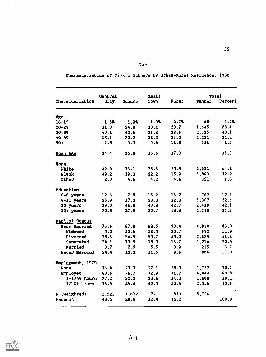
Table 1 presents data on several characteristics of single

mothers in this sample, for both the total group and the four

rural-urban residential areas. By far the largest proportion of

single mothers live in central cities (43.5 percent), followed by

residence in suburban areas (28.9 percent). Much smaller groups

live in rural areas (15.2 percent) and small towns (12.4 percent).

Comparing the residential areas, several differences in

characteristics are clear. While the average age of all single

mothers is 35.3 years, mothers residing in central cities are

35

7:412:1

Characteristics of St-14; Hothers by Urban-Rural Residence, 1980

CharacteristicsCentral

City SuburbSmallTown Rural

TotalNumber Percent

Age16-19 1.5% 1.0% 1.0% 0.7% 68 1.2%

20-29 31.9 24.9 30.1 23.7 1,645 28.4

30-39 40.1 42.6 36.3 38.6 2,325 40.1

40-49 18.7 22.2 23.2 25.2 1,231 21.2

50* 7.8 9.3 9.4 11.8 526 8.5

Mean Age 34.4 35.8 35.6 37.0 35.3

RaceWhite 42.8 76.1 73.6 79.5 3,581 61.8

Black 49.2 19.3 22.2 15.9 1,863 32.2

Other 8.0 4.6 4.2 4.6 351 6.0

Education0-8 years 12.6 7.9 15.2 16.2 702 12.1

9-11 years 25.9 17.3 23.3 22.3 1,307 22.6

12 years 39.0 46.9 40.8 42.7 2,439 42.1

13+ years 22.5 27.9 20.7 18.8 1,348 23.3

Mar426:1 Status75.6 87.8 88.5 90.4 4,810 83.0Ever Married

Widowed 9.2 10.6 13.9 20.7 692 11.9

Divorced 38.6 54.9 50.7 49.0 2,689 46.4

Separated 24.1 19.5 18.3 16.7 1,214 20.9

Married 3.7 2.9 5.5 3.9 215 3.7

Never Married 24.4 12.2 11.5 9.6 986 17.0

Employment, 1979None 36.4 23.3 27.1 28.3 1,752 30.2

Employed 63.6 76.7 72.9 71.7 4,044 69.8

1-1749 hours 27.2 30.3 30.6 31.3 1,688 29.1

1750+ tlurs 36.5 46.4 42.3 40.4 2,356 40.6

N (weighted) 2,523 1,672 721 879 5,796

Percent. 43.5 28.9 12.4 15.2 100.0

36

younger, on average, than mothers in other areas. Rural mothers are

oldest of the four groups, with 37.0 percent age 40 and older, and

an average age of 37.0 years.

About 62 percent of all single mothers are white, and 38 percent

are nonwhite. The racial distribution of single mothers in central

cities is markedly different from that in other areas. Over half of

all central city single mothers ariv nonwhite, with most being

black. In the other residential areas, the proportion of nonwhite

single mothers is one-fourth at most.

About 65 percent of all single mothers have completed high

school. Suburban single mothers have higher educational attainment

than mothers from other residential areas, with 75 percent being

high school graduates. The mothers living in the other three

residential areas have very similar educational attainment, with

about 60 percent high school graduates in each area.

Overall, four-fifths of single mothers have ever been married;

almost half of all single mothers are divorced. Central city

mothers are much less likely to have ever married than mothers

living in other areas; three-fourths of central city mothers have

been married, while 88 to 90 percent of all zAher single mothers

have been married. The proportion divorced is highest among

suburban mothers, while wi*mhood is most prevalent among rural

single mothers. This latter status probably reflects the older

average age of rural mothers.

Seventy percent of all single mothers were employed during 1979,

37

with 40.6 percent being employed full time (as defined by working

1750 or more hours in that year). Proportions employed during 1979

also vary by residential area. The greatest employment is among

suburban single mothers (76.7 percent), followed by small town (72.9

percent) and rural (71.7 percent) mothers, while central city

mothers have the lowest levels of employment (63.6 percent).

Suburban mothers are also more likely to be employed full time than

mothers in other areas.

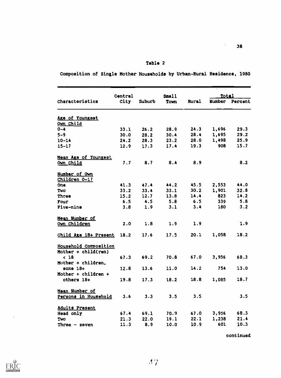
The characteristics of the entire single mother household are

deemed important in this research. Table 2 presents information

about the composition of these households, again for four

residential types as well as for the total sample.

Almost 30 percent of all single mothers have a preschool age

child -- that is, age 4 or younger. Central city single mothers are

most likely to have a preschool child. Given the older age

distribution of rural mothers, it is not surprising to find that a

larger proportion of them have no child younger than 15. The mean

age of youngest child reflects these differences in age distribution

of youngest child.

Forty-four percent of single mothers have one minor child living

with them, 33 percent have two, and 23 percent have three or more.

Suburban mothers are more likely than others to have only one child

(47.4 percent). Central city mothers are more likely to have three

or more children, followed by rural mothers. This is reflected in

the mean number of children: central city mothers have the largest

38

Table 2

Composition of Single Mother Households by Urban-Rural Residence, 1980

CharacteristicsCentral

City SuburbSmallTown Rural

TotalNumber Percent

Age of YoungestOwn Child0-4 33.1 26.2 28.9 24.3 1,696 29.3

5-9 30.0 28.2 30.4 28.4 1,695 29.2

10-14 24.2 28.3 23.2 28.0 1,498 25.9

15-17 12.9 17.3 17.4 19.3 908 15.7

Mean Age of YoungestOwn Child 7.7 8.7 8.4 8.9 8.2

Number of OwnChildren 0-17One 41.3 47.4 44.2 45.5 2,553 44.0

Two 33.2 33.4 33.1 30.2 1,901 32.8Three 15.2 12.7 13.8 14.4 823 14.2

Four 6.5 4.5 5.8 6.5 339 5.8

Five-nine 3.8 1.9 3.1 3.4 180 3.2

Mean Number ofOwn Children 2.0 1.8 1.9 1.9 1.9

Child Age 18+ Present 18.2 17.6 17.5 20.1 1,058 18.2

Household CompositionMother + child(ren)

< 18 67.3 69.2 70.8 67.0 3,956 68.3

Mother + children,some 18+ 12.8 13.6 11.0 14.2 754 13.0

Mother + children +others 18+ 19.8 17.3 18.2 18.8 1,085 18.7

Mean Number ofPersons in Household 3.6 3.3 3.5 3.5 3.5

Adults PresentHead only 67.4 69.1 70.9 67.0 3,956 68.3

Two 21.3 22.0 19.1 22.1 1,238 21.4

Three - seven 11.3 8.9 10.0 10,9 601 10.3

continued

7

39

Tabli 2, continued

Total Adult EarnersNone 30.1 18.2 20.9 21.1 1,401 24.2

One 52.9 60.4 60.5 58.2 3,292 56.8

Two - five 17.0 21.4 18.6 20.7 1,104 19.0

N (weighted) 2,523 1,672 721 879 5,796

Percent 43.5 28.9 12.4 15.2 100.0

40

average number of children, suburban mothers the smallest, and small

town and rural mothers fall in between. Overall, these data preseni

the picture of suburban mothers more likely to have just one child,

central city mothers more likely to have se4eral young children, and

rural mothers to have teenagers.

Almost one fifth of all single mother households have an adult

child present -- that is, a child of the mother who is age 18 or

older. Rural households are more likely to have an adult child

present than are the other areas.

The household composition variable summarizes persons living in

the household with the mother. By definition, all of these

households contain at least one minor child along with the single

mother. Over two-thirds of all households contain a mother with

only minor children. The second largest group consists of

households with minor children plus another adult besides the mother

-- almost 20 percent of all households are in this group. The

smallest proportion of households (13.0 percent) consists of mothers

living with both minor and adult children (age 18+). There are no

large differences between residential areas for this variable.

Small town mothers are most likely to be living with only minor

children; central city mothers are somewhat more likely to be living

with another adult.

The mean number of persons in these households is 3.5 overall.

Central city hous...holds are largest on average, with 3.6 persons,

followed by small town and rural households with 3.5 persons each,

41

and finally suburban households with 3.3 persons. Subtracting

average number of own children from average household size, there is

an average of about 1.6 persons other than own children in these

households. One person, of course, is the single mother. The

remaining 0.6 person is an adult who is not a child of the mother,

or one of very few unrelated minor children in these households.

Another way of looking at household composition is to consider

number of adults present. In two-thirds of these households, the

single mother is the sole adult. About one-fifth of single mother

households have two adults present, and one-tenth have three or more

adults. The variations between urban and rural areas are not great;

suburban and small town mothers are slightly more likely to be the

only adult, while central city and rural mothers are slightly more

likely to have another adult present. Central city mothers are most

likely to live with two or more additional adults.

In an analysis of adult earners not shown here, it was found

that over 99 percent of adult earners were employed during 1979.

Thus, the correlation between earning income end employment is

extremely high. It was decided to use earners as the variable for

analysis here because poverty status is related to income more

directly than it is to employment. Any small error in reporting

employmept is avoided with tAis choice.

Number of adults who earned any income during 1979 is also shown

in Table 2; note that this variable includes the single mother plus

any adults living with her. Urned income includes wages, salaries,

51)

42

and self-employment income. About one-fourth of all households have

no adults earning income in 1979, and three-fourths have one or more

earners. Within residence areas, central city households are least

likely to have adults earning income. Rural, small town, and

suburban households have similar proportions with adult earners --

approximately 80 percent. The majority of households with an adult

earner have just one; again, the proportion of central city

households with one earner is lower than for the other three

residence areas.

If only households with an extra adult present are analyzed,

this pattern changes slightly (data nct shown in Table 2). Central

city households are still least likely to have an extra adult

earning income (68.6 percent), followed by rural households (76.6

percent), then small town households (80.2 percent). Suburban

households continue to be most likely to have an extra earner (81.2

percent).

Poverty status is the dependent variable for this research.

Table 3 shows poverty status by area of residence for all single

mother families. Overall, 31.0 percent of all families are very

poor -- their 1979 income is below 75 percent of the poverty

threshold. The depth of poverty is greatest in central cities, with

35.4 percent being very poor. This is followed by small townq (32.7

percent) and rural areas (31.5 percent), while 23.4 percent of

suburban families experience this level of poverty. Another 11

percent of all families are in the 75-99 percent of poverty

43

Table 3

Poverty Status of Single Mother Familiesby Urban-Rural Residence, 1979

Poverty StatusCentral

City SuburbSmallTown Rural

TotalNumber Percent

< 75% 35.4 23.4 32.7 31.5 1,798 31.0

75-99 12.1 9.4 11.8 9.7 635 10.9

100-124 8.4 6.9 10.4 10.9 499 8.6

125-149 7.6 6.9 9.4 7.6 443 7.6

150-174 6.4 7.2 8.4 7.4 408 7.0

175-199 5.0 8.3 4.7 6.6 359 6.2

200+ 24.9 37.8 22.5 26.2 1,654 28.5

N (weighted) 2,523 1,672 721 879 5,796

Percent 43.5 28.9 12.4 15.2 100.0

44

threshold group. Thus, a total of 42 percent of all single mother

families fall below the poverty threshold. As an example of how

this translates into money income, for a family of three persons,

including two minor children, an income of $5844 or less in 1979 is

below the poverty threshold.

At the other extreme, 28.5 percent of all families had income of

at least 200 percent of the poverty threshold. Again there are

differences by area, with suburban families much more likely to be

well off -- 37.8 percent have this level of income. The other three

residence groups are closer to 25 percent each with incomes at or

above the 200 percent threshold. Small town families are the least

likely to have higher family incomes (22.5 percent are at 200

percent of poverty threshold).

Poverty Status and Characteristics of Sinxle Mother Households

This section focuses on findings related to the dependent

variable, poverty status, and provides preliminary evidence

regarding the five hypotheses. For the total group, Table 4 asain

indicates that central city residents are most likely to be poor

(47.6 percent), followed by small town (44.6 percent) and rural

residents (41.2 percent). Suburban residents are least likely to be

poor (32.8 percent). This provides partial confirmation for

Hypothesis 1, which states that poverty in urban areas is lower than

it is in rural areas. Although central city residents are poorer

than any other group, a combined urban group (central city and

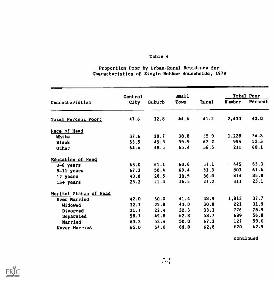
Table 4

Proportion Poor by Urban-Rural Residence forCharacteristics of Single Mother Households, 1979

Characteristics

CentralCity Suburb

SmallTown Rural

Total PoorNumber Percent

Total Percent Poor: 47.6 32.8 44.6 41.2 2,433 42.0

Race of Head

White 37.6 28.7 38.8 35.9 1,228 34.3

Black 53.5 45.3 59.9 63.2 994 53.3

Other 64.4 48.5 65.4 56.5 211 60.1

Education of Head0-8 years 68.0 61.1 60.6 57.1 445 63.3

9-11 years 67.3 50.4 69.4 51.3 803 61.4

12 years 40.8 28.5 38.5 36.0 874 35.8

13+ years 25.2 21.3 16.5 27.2 311 23.1

Mavital Status of Head42.0 30.0 41.4 38.9 1,813 37.7Ever Married

Widowed 32.7 25.8 43.0 30.8 221 31.9

Divorced 31.7 22.4 32.3 33.3 776 :8.9

Separated 58.7 49.8 62.8 58.7 689 56.8

Married 63.3 52.4 50.0 67.2 127 59.0

Never Married 65.0 54.0 69.0 62.8 620 62.9

continued

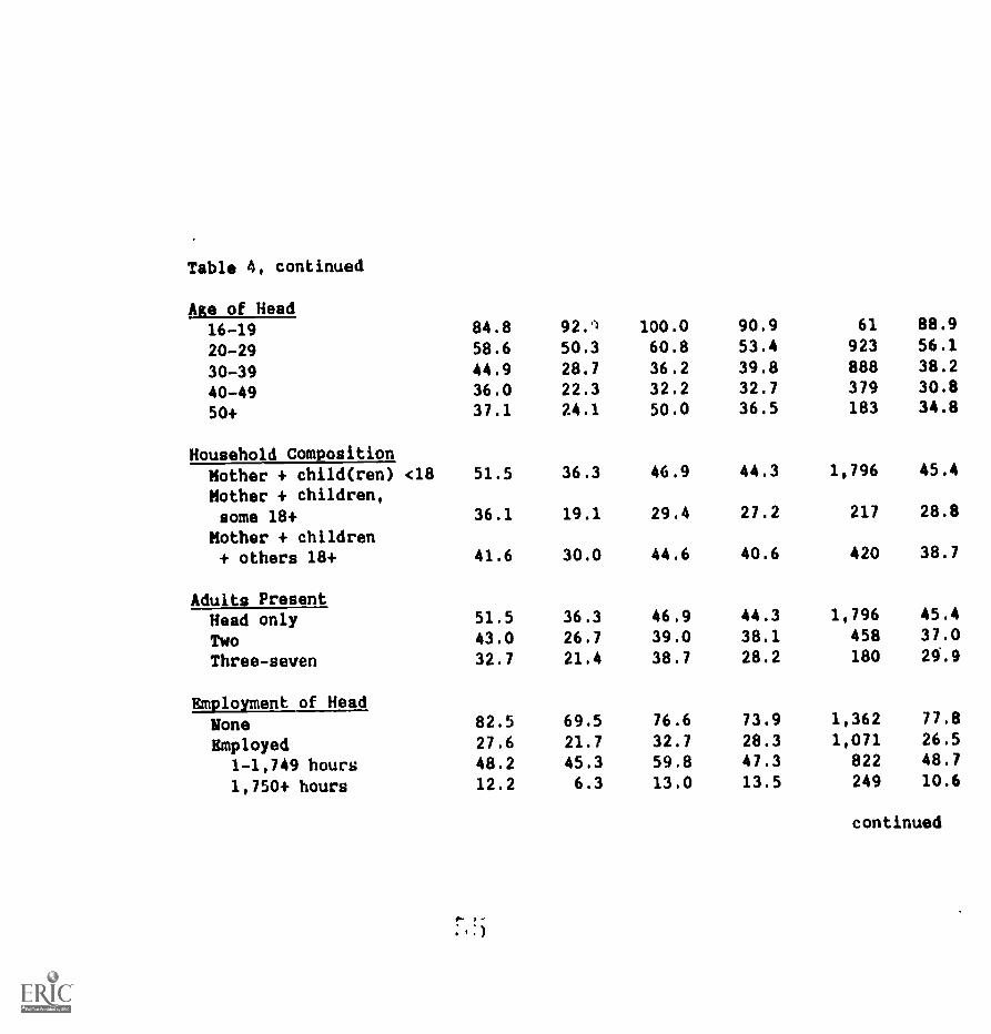
Table 4, continued

Age of Head16-19

20-29

30-3940-4950+

Household Composition<18

84.8

58.6

44.936.037.1

51.5

36.1

41.6

51.5

43.032.7

82.5

27.6

48.2

12.2

92.1

50.3

28.7

22.324.1

36.3

19.1

30.0

36.3

26.7

21.4

69.5

21.7

45.3

6.3

100.060.8

36.232.2

50.0

46.9

29.4

44.6

46.939.0

38.7

76.6

32.7

59.813.0

90.9

53.439.832.736.5

44.3

27.2

40.6

44.3

38.128.2

73.9

28.347.313.5

61

923

888

379183

1,796

217

420

1,796

458180

1,362

1,071822249

88.9

56.138.2

30.834.8

45.4

28.8

38.7

45.437.024.9

77.8

26.5

48.7

10.6

Mother + child(ren)Mother + children,some 18+

Mother + children+ others 18+

Adults PresentHead onlyTwoThree-seven

Employment of Head

None

Employed1-1,749 hours1,750+ hours

continued

Table 4, continued

Total Adult EarnersNone 89.7 78.9 86.8 81.1 1,204 85.9

One 31.9 25.6 36.2 34.6 1,108 30.9

Two-five 21.9 14.3 24.6 19.2 213 19.3

N (weighted) 2,523 1,672 721 879 5,796

Percent 43.5 28.9 12.4 15.2 100.0

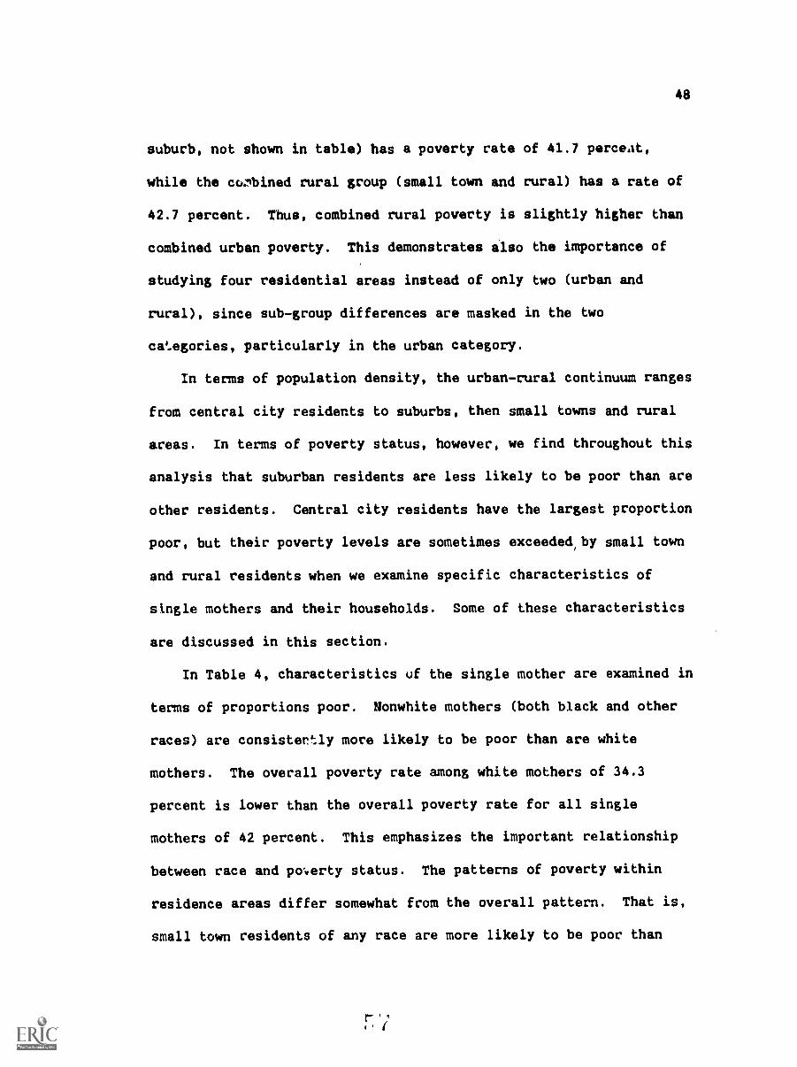
48

suburb, not shown in table) has a poverty rate of 41.7 perceat,

while the ccobined rural group (small town and rural) has a rate of

42.7 percent. Thus, combined rural poverty is slightly higher than

combined urban poverty. This demonstrates also the importance of

studying four residential areas instead of only two (urban and

rural), since sub-group differences are masked in the two

ca'..egories, particularly in the urban category.

In terms of population density, the urban-rural continuum ranges

from central city residents to suburbs, then small towns and rural

areas. In terms of poverty status, however, we find throughout this

analysis that suburban residents are less likely to be poor than are

other residents. Central city residents have the largest proportion

poor, but their poverty levels are sometimes exceeded,by small town

and rural residents when we examine specific characteristics of

single mothers and their households. Some of these characteristics

are discussed in this section.

In Table 4, characteristics uf the single mother are examined in

terms of proportions poor. Nonwhite mothers (both black and other

races) are consistertly more likely to be poor than are white

mothers. The overall poverty rate among white mothers of 34.3

percent is lower than the overall poverty rate for all single

mothers of 42 percent. This emphasizes the important relationship

between race and po.verty status. The patterns of poverty within

residence areas differ somewhat from the overall pattern. That is,

small town residents of any race are more likely to be poor than

49

central city residents; among black mothers, rural women are much

more likely to be poor than their central city counterparts. As

always, suburban women are least likely to be poor.

Proportions poor drop as educational attainment increases. The

greatest decrease in proportion poor is found with attainment of a

high school diploma -- proportion poor decreases by more than 25

percent in the overall group. Within residence areas, a very

similar pattern holds true. Among mothers with the least education,

central city mothers have much higher rates of poverty than the

others, and rural women are somewhat lower. This may be a

reflection of age differences among these groups, with the older

rural women more able to obtain employment and income in spite of

low education levels. It may also reflect racial differences and

unequal access to employment and income. Interestingly, at the

highest education levels, small town women actually have a lower

proportion poor than suburban women. The small number in this

group, however, may give misleading results.

In terms of marital status and poverty, two groups emerge. High

poverty levels are found among separated, married,1

and never

married women. Lower than average poverty rates are found among

widowed and divorced women. This difference seems to be related to

nature of the mother's relationship with the father of her children,

or with her former husband. Both widows and divorced women have

formal, legal relationships to their husbands and, to some degree,

to their husbands' income. Never married and separated women have

50

no such legal relationships. Within the four residence areas,

suburban mothers have the lowest levels of poverty for all marital

status groups. As noted before, divorced women are the largest

marital status group among single mothers. About one-third of

central city, small town, and rural mothers who are divorced are

poor, while only 22 percent of suburban divorced women are poor.

Poverty rates decline with increasing age; only when single

mothers reach age 50 is there a reversal of this trend. The

greatest decrease in poverty levels occurs with single mothers age

30-39 -- they are much less likely to be poor than are mothers age

20-29. Some of the highest poverty rates found in this research

occur among teenage single mothers -- 85 percent or more of these

women are poor, varying with residence area. In this sample,

however, this group is quite small.

The household composition variable provides evidence in support

of Hypothesis 2: households with an extra adult are less likely to

be poor than those with only the single mother. (Note that poverty

status applies only to family members within the household.) In all

four residence areas, highest poverty rates are observed in

households with only minor children, and poverty rates are lower for

households with an extra adult present -- whether that adult is a

child of the head or not. The lowest rates of poverty are observed

in households with an adult child present. Apparently, in some

cases an extra adult is more likely to be an economic burden; more

so when the adult is not a child of the head.

51

The presence of extra adults in the household also provides

evidence for Hypothesis 2. Poverty rates are lower when another

adult in addition to the single mother lives in the household. And

poverty rates continue todecline when three Dr more adults are

present. Hypothesis 2A can be examined with these data; in

households with an extra adult, are urban poverty rates lower than

rural ones? The answer is no, except in the case of suburban

households. Central city households with two adults present are

more likely to be poor than are rural or small town households.

When three or more adults are present small town households are

poorest, but central city households are more likely to be poor than

are rural households.

Employment of the single mother provides verification for

Hypothesis 3, as shown in Table 4. Without exception, employment is

associated with lower poverty rates and, conversely, being outside

the labor force is associated with the highest levels of poverty.

While this is not surprising, it is .eresting to note both the

strength of this association and the variations rcs residence

types. Part-time employment of the single mother head during 1979

brings the family poverty rate down to 48.7 percent, and when she is

employed full time the overall poverty rate drops to 10.6 percent.

These rates can be contrasted with the overall poverty rate of 42

percent, and witil -1,most 78 percent poverty when the mother is not

employed. Across the four residence groups the same relationships

hold true. Suburban residents have the lowest poverty rates;

52

central city residents have the highest poverty rates when the head

is not employed. Of special interest here is that small town and

rural residents share the distinction of having highest poverty

rates when the single mother is employed. The fact that almost 60

percent of small town mothers who work part time are poor is

especially striking. There is a selection bias inherent in this

relationship. Women who have the skills necessary to obtain

employment are more likely to be employed, leaving the least

employable women out of the labor force, and thus more likely to be

poor.

The relationships between number of adults earning income in

1979 and poverty status also help confirm Hypothesis 3. Households

with no adults earning income in 1979 have the highest poverty

levels while households with one adult earner have poverty rates

below 37 percent. Only 25.6 percent of suburban households with one

adult earner are poor. Presence of two or more earners is related

to even lower poverty rates -- less than 25 percent everywhere, and

less than 20 percent in rural areas and suburbs.

The evidence in support of Hypothesis 3A is also presented in

Table 4. Hypothesis 3A states that, among households with employed

adults, urban poverty levels are lower than rural ones. As noted

earlier, poverty rates for employed single mothers heads are

consistently lower than those of mothers who are nnt employed,

across all four residence groups. In terms of full time employed

mothers (working 1750 or more hours), poverty rates in urban areas

53

are lower than rates in rural areas: 12.2 percent of full time

workers in central cities are poor, and 6.3 percent in suburbs,

while small town and rural mothers have rates of 13.0 percent and

13.5 percent, respectively. The picture is somewhat less clear for

part time working mothers. Highest poverty rates are experienced by

small town mothers (59.8 percent), but this is followed by central

city (48.2 percent) and then rural mothers (47.3 percent). Suburban

mothers, as always, have the lowest poverty rate, at 45.3 percent.

Thus, the poverty rates for employed mothers give partial support to

Hypothesis 3A.

Poverty rates for households with one adult earner (including

the head) give some further support to Hypothesis 3A. When there is

one adult earner in the household, small town and rural households

have the highest poverty rates (36.2 and 34.6 percent respectively),

followed by central city (31.9 percent) and suburban households

(25.6 percent). The pattern changes, however, in households with

two or more adults earning income. Highest poverty rates are found

in small town households, followed by central cities. Thus, the

evidence for Hypothesis 3A is mixed. It appears that central cities

are more similar to rural areas than they are to suburban areas when

earned income and poverty are examined. This question will be

raised again with the multivariate analysis, to see whether

controlling for sociodemographic characteristics will yield a

different outcome.

54

Multivariate Anal;

This section includes the specification and estimation of all

multivariate models, in order to test the five hypotheses. In all

models, four variables are included to control for the effects of

socioeconomic variables presented in the previous section: race,

education, marital status and age of mother.

The first hypothesis -- that poverty eates are lower in urban

than in rural areas -- is tested with a multivariate model using

multiple classification analysis (MCA), in ortler that proportion

poor may be compared between models for the four residence areas

with and without controls. The dependent variable is poverty

status, coded as a dichotomous v&Aable: poor and nonpoor. The

results are presented in Table 5.

The column labeled "Unadjusted Percent" in Table 5 presents the

proportion in poverty for each independent variable. These results

are the same as proportions poor shown in Table 4. The "Adjusted

Percent" column presents the proportion in poverty for each

variable, controlling for all the other independent variables in the

model.

The proportion poor in central cities, controlling for race,

education, maritai status and age, drops from 48 to 43 percent2

when other variables in the model are controlled. The proportion

poor in suburbs is 38 percent in the multivariate model,

considerably higher than the 33 percent poor in the simple model.

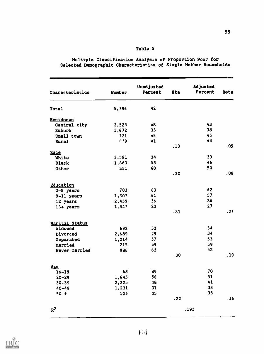
55

Table 5

Multiple Classification Analysis of Propoction Poor forSelected Demographic Characteristics of Single Mother Households

Characteristics NumberUnadjusted

Percent EtaAdjustedPercent Beta

Total

Residence

5,796

2,5231,672

42

48

33

4338

Central citySuburbSmall town 721 45 45

Rural P79 41 43.13 .05

RaceWhite 3,581 34 39

Black 1,863 53 46

Other 351 60 50

.20 .08

Education0-8 years 703 63 62

9-11 years 1,307 61 57

12 years 2,439 36 36

13+ years 1,347 23 27

.31 .27

Marital StatusWidowed 692 32 34

Divorced 2,689 29 34

Separated 1,214 57 53

Married 215 59 59

Never married 986 63 52

.30 .19

ALft16-19 68 89 70

20-29 1,645 56 51

30-39 2,325 38 41

40-49 1,231 31 33

50 + 526 35 33

.22 .16

R2 .193

G

56

Proportions poor in small town and rural areas are 45 and 43 percent

respectively in the multivariate model. Thus, the proportions poor

in rural areas -- including small towns -- are equal to or higher

than the proportions poor in cities and suburbs, when controlling

for race, education, marital status and mother's age. These

findings provide confirmation of Hypothesis 1.

Hypothesis 2 states that households with more than one adult are

less likely to be poor than those with only one adult, i.e., the

single mother. This is tested with multiple classification

analysis; results are presented in Table 6. Only adjusted percents

are presented in this table; as noted earlier, the unadjusted

percents are identical to those included in Table 4. This table

provides clear and unequivocal evidence in support of Hypothesis 2.

For all four residence areas as well as for the total group, the

presence of extra adults is associated with lower poverty levels,

controlling for the effects of race, education, marital status and

age. Overall, the adjusted percent poor for households with two or

more adults is 35 percent while 45 percent of households with one

adult are poor. The pattern is.similar in the four residence areas;

the difference in proportion poor between households with one and

two or more adults is eight or more percentage points. In

comparison with the grand mean for each residence area, households

with on, Adult are always more likely to be poor, and households

with an extra adult are always less likely to be poor.

Hypothesis ZA posits that, in households with an extra adult

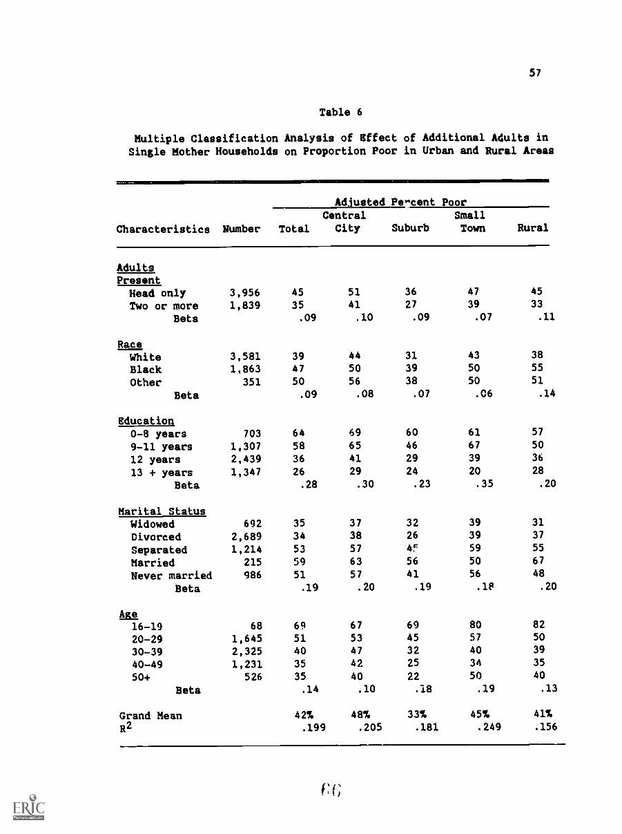
57

Table 6

Multiple Classification Analysis of Effect of Additional Adults inSingle Mother Households on Proportion Poor in Urban and Rural Areas

Characteristics Number

Adiusted Pe.-cent Poor

Total

CentralCity Suburb

SmallTown Rural

AdultsPresent

Head only 3,956 45 51 36 47 45

Two or more 1,839 35 41 27 39 33

Beta .09 .10 .09 .07 .11

RaceWhite 3,581 39 44 31 43 38

Black 1,863 47 50 39 50 55

Other 351 50 56 38 50 51

Beta .09 .08 .07 .06 .14

Education0-8 years 703 64 69 60 61 57

9-11 years 1,307 58 65 46 67 50

12 years 2,439 36 41 29 39 36

13 + years 1,347 26 29 24 20 28

Beta .28 .30 .23 .35 .20

Marital StatusWidowed 692 35 37 32 39 31

Divorced 2,689 34 38 26 39 37

Separated 1,214 53 57 4f 59 55

Married 215 59 63 56 50 67

Never married 986 51 57 41 56 48

Beta .19 .20 .19 .1S .20

Age16-19 68 69 67 69 80 82

20-29 1,645 51 53 45 57 50

30-39 2,325 40 47 32 40 39

40-49 1,231 35 42 25 34 35

50+ 526 35 40 22 50 40

Beta .14 .10 .18 .19 .13

Grand Mean 42% 48% 33% 45% 41%

R2 .199 .205 .181 .249 .156

(4;

58

present in addition to the single mother, urban poverty rates will

be lower than rural poverty rates. Multiple classification analysis

results shown in Table 6 provide mixed evidence. Among households

with more than one adult, suburban households have the lowest

poverty rate, 27 percent. The next lowest rate, however, is found

in rural households with 33 percent poor, followed by small town

with 39 percent poor, and the highest rate is among central city

households with 41 percent poor. Thus, central city households do

not conform to the hypothesis.

Hypothesis 3 states that households with employed members are

less likely to be poor than those with no employed members. This is

tested with multiple classification analysis using number of adults

earning income during 1979 as the independent variable of interest.

The distribution of this variable is shown in Table 2; MCA results

are in Table 7A. The proportion poor, controlling for effects of

other variables, is indeed much smaller in households with adult

earners. This is true for all residence areas as well as for the

total group. The decrease in proportion poor between households

with no earners and those with one earner is dramatic: 78 percent

of all households with no adult earner are poor, while 33 percent of

households with one adult earner are poor. The smallest decline in

proportion poor occurs in small town households, but even there the

difference in proportions poor is 36 percent. Thus Hypothesis 3 is

confirmed without reservation.

It is possible, witb these data, to examine the effects of

f;

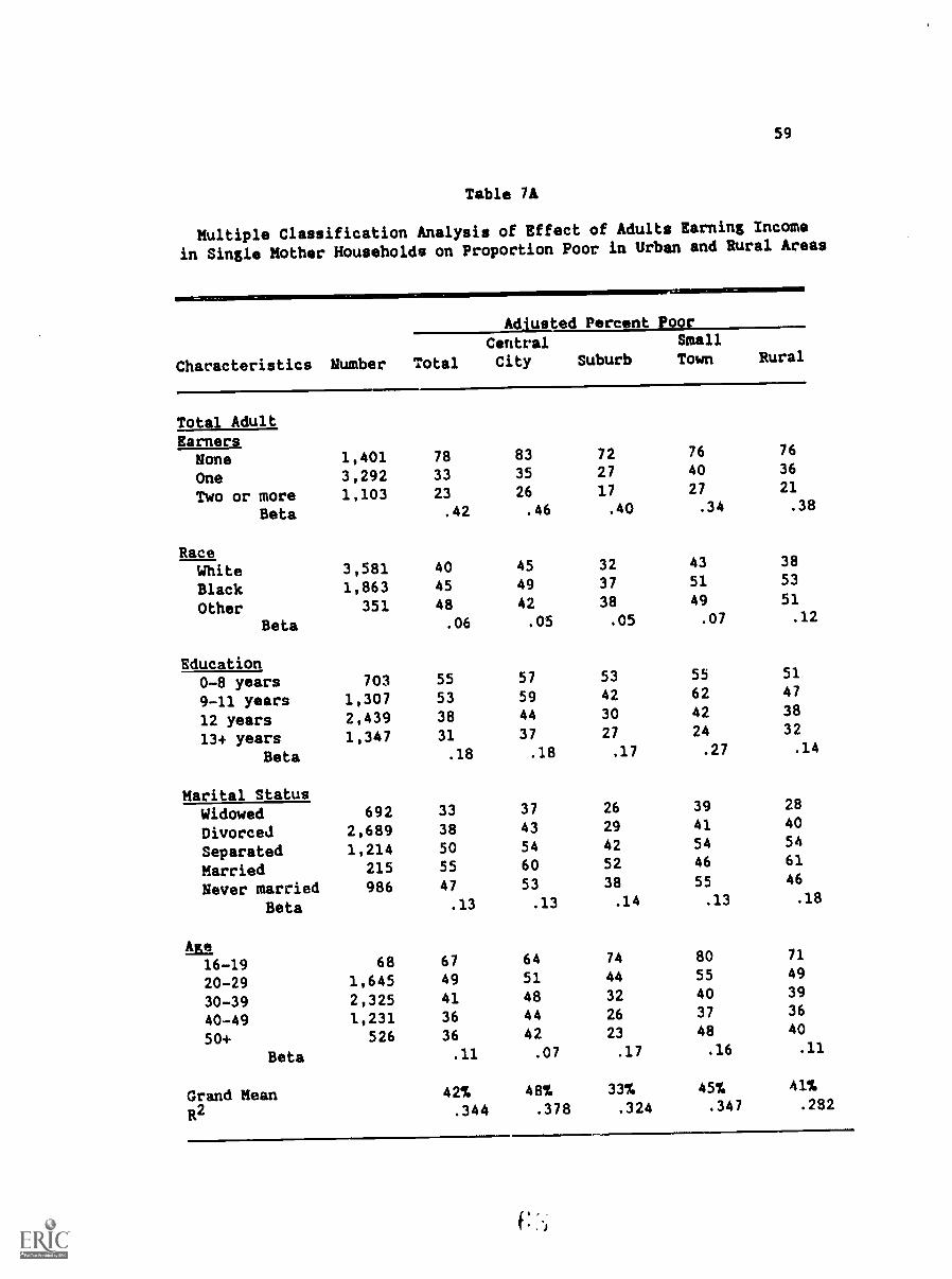
59

Table 7A

Multiple Classification Analysis of Effect of Adults Earning Income

in Single Mother Households on Proportion Poor in Urban and Rural Areas

cow

Adiusted Percent Poor

Central Small

Characteristics Number Total City Suburb Town Rural

Total AdultEarners

None 1,401 78 83 72 76 76

One 3,292 33 35 27 40 36

Two or more 1,103 23 26 17 27 21

Beta .42 .46 .40 .34 .38

RaceWhite 3,581 40 45 32 43 38

Black 1,863 45 49 37 51 53

Other 351 48 42 38 49 51

Beta .06 .05 .05 .07 .12

Education0-8 years 703 55 57 53 55 51

9-11 years 1,307 53 59 42 62 47

12 years 2,439 38 44 30 42 38

13+ years 1,347 31 37 27 24 32

Beta .18 .18 .17 .27 .14

Marital StatusWidowed 692 33 37 26 39 28

Divorced 2,689 38 43 29 41 40

Separated 1,214 50 54 42 54 54

Married 215 55 60 52 46 61

Never married 986 47 53 38 55 46

Beta .13 .13 .14 .13 .18

A6116-19 68 67 64 74 80 71

20-29 1,645 49 51 44 55 49

30-39 2,325 41 48 32 40 39

40-49 1,231 36 44 26 37 36

50+ 526 36 42 23 48 40

Beta .11 .07 .17 .16 .11

Grand Mean 42% 48% 33% 45% 41%

R2 .344 .378 .324 .347 .282

60

specific adults' employment on poverty status. As shown in Table 4,

the employment of the single mother was strongly related to

decreasing poverty status. In Table 7B the adults with earned

incomo are separated into two groups: household heads and all other

adults. Employment of the head, controlling for other adult earners

and sociodemographic characteristics, is strongly related to reduced

poverty levels. Overall, 73 percent of all households are poor when

tho head is not employed, 49 percent are poor when the head is

employed part time, and only 14 percent are poor when the head is

employed full time. Results are similar in all four areas:

proportion poor declines sharply with employment of the head, and

even more so when the h.ad is employed full time. Indeed, when the

head was employed full time (1750 or more hours), poverty rates

dropped below 20 percent -- a very unusual occurrence in this

population. The weakest effect of head employment is seen in small

town households; 59 percent of these households remain poor when the

head is employed part time. This is the highest poverty level among

all households with part time employed heads. Among households with

head employed full time in 1979, the highest proportion poor is

again found in small towns (19 percent). This is followed by

central city households with 17 percent poor when head is a full

time employee, rural households at 14 percent poor, and suburban

households with only 9 percent poor. The Beta statistics indicate

that employment of the head is by far the most important variable in

this model. Although MCA does not indicate proportion of variance

61

Table 78

Multiple Classification Analysis of Effect of Labor Force Variableson Poverty in Single Mother Households in Urban and Rural Areas

Characteristics Number

Adjusted Percent Poor

TotalCentralCity Suburb

SmallTown Rural

Head EmploymentNone 1,752 73 78 66 70 73

1-1749 hours 1,688 49 49 44 59 48

1750+ hours 2,356 14 17 9 19 14

Beta .50 .52 .50 .46 .50

Other Adult EarnersNo other adults 3,952 45 51 36 47 45

No other earners 467 49 53 43 63 46

Other adult earners 1,377 32 37 23 35 30

Beta .12 .12 .12 .14 .13

RaceWhite 3,581 40 45 31 43 38

Black 1,863 46 49 39 50 53

Other 351 47 53 34 47 49

Beta .06 .05 .07 .05 .12

Education0-8 years 703 52 53 50 54 48

9-11 years 1,307 51 57 39 61 45

12 years 2,439 40 46 31 42 40

13+ years 1,347 32 39 27 26 33

Beta .15 .14 .14 .24 .10

Marital StatusWidowed 692 28 34 19 36 23

Divorced 2,689 40 45 32 42 40

Separated 1,214 49 52 40 54 29

Married 215 52 58 46 47 58

Never married 986 47 53 37 54 37

Beta .13 .12 .13 .13 .21

continued

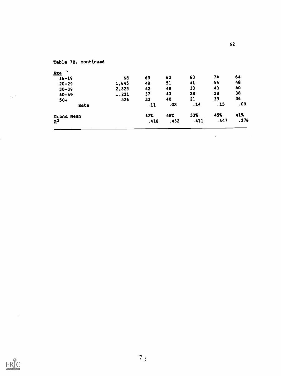
62

Table 7B, continued

Alt16-19 68 63 63 63 74 64

20-29 1,645 48 51 41 54 48

30-39 2,325 42 49 33 43 40

40-49 J,231 37 43 28 38 38

50+ 526 33 40 21 39 36

Beta .11 .08 .14 .13 .09

Grand Mean 42% 48% 33% 45% 41%

R2 .418 .432 .411 .447 .376

63

explained by each independent variable, it is clear that the

mother'r employment plays a very large role in determining poverty

status.

Similar results occur with analysis of employment among other

adults in the household. As noted earlier, adults with earned

income represent employed adults. When other adults are present,

but not earning income, the overall poverty rate is 49 percent.

When another adult is earning, the proportion poor drops to 32

percent. Within residence areas the central city and small town

households are more likely to remain poor when another adult ts

earning income. The Beta statistic indicates that this variable is

relatively less important than the head's employment. It is

important to note, however, that the pattern of increasing

employment related to decreasing poverty levels is maintained when

adults in the households are separated into two groups.

Hypothesis 3A states that, among households with one or more

employed adult, poverty rates in urban areas are lower than those in

rural areas. This is operationalized with a model including the

four control variables, plus the number of adult earners in the

household. Multiple classification analysis results are presented

in Table 7A.

Small town and rural households with one earner have higher

proportions poor than central city or suburban households, thus

partially confirming the hypothesis. When two or more adults

earning income are present, small town and central city households

64

have the highest proportions poor. Since these results do not

completely support the hypothesis, we turn to Table 78 for

additional information. The results for employment of head and

other adult earners do not provide confirmation of Hypothesis 3A.

In general, in households with employed heads, poverty rates are

highest in small towns, followed by central cities. The reverse is

true for households with other adults employed: proportion poor is

highest for central city cases, followed by small towns and then

rural areas. Only in the suburban households, with consistently the

lowest poverty levels, do we find evidence that urban poverty is

lower overall than rural poverty.

A multiple regression analysis of these variables was conducted

to estimate regression coefficients, and thus learn more about their

relationship to poverty status. The dependent variable is the

income-needs ratio, ranging in value from 0 to 1500 with a mean of

153.5. This variable is the Census poverty status, recalculated by

dividing 1979 family income by the poverty threshold appropriate to

that family size, then dividing by 100. The poorer a family, the

smaller the income-needs ratio, and vice versa. Families with an

income-needs ratio of 100 or more are not poor. The first

regression model estimated includes the sociodemographic control

variables alcng with residence areas. Race is coded dichotomously:

white and nonwhite. Marital status is coded as five dummy

variables, omitting the category of "nevev married" to avoid

problems with multicollinearity. Age and education of mother are

65

coded in single year increments. Area of residence is coded as four

dummy variables, with suburbs omitted, again to avoid

multicollinearity.

Results are presented as Model 1 in Table 8. The negative

coefficient for race indicates that the average income-needs ratio

is lower for nonwhites than for whites, controlling for the effects

of education, marital status, age and residence. A one-year

increase in educational attainment is associated with a 14-point

increase in the income-needs ratio, controlling for the effects of

the other variables in the model. The dummy variable coefficients

for marital status indicate that widowed and divorced mothers are

better off than the omitted category of never married mothers, while

separated and married (spouse absent) mothers are worse off. For

example, the mean income-needs ratio for widowed mothers is almost

30 points greater than the mean for never married mothers. Thc

coefficient for age indicates that a one-year increase in age is

associated with a modest 3-point increase in the dependent variable,

controlling for race, education, marital status and residence

effects. The coefficients for the dummy variables for residence

compare the difference in mean income-needs ratio to the omitted

category of suburban residents. Small town and rural residents are

least well off, with a mean ratio more than 30 points lower than the

suburban mean. Model 1 accounts for 21.6 percent of the variance in

the income-needs ratio.

Model 2 includes the number of adults present in addition to the

Table 8

Multiple Regression Analysis of the Effect of Adults and Employed Persons on Income-Needs

Ratio for Single Mother Households in Urban and Rural Areas, 1979 (n=5,796)

Independent

Variables

Model 1 Model 2 Model 3

RegressionCoefficient

StandardizedCoefficient

Rwession..Aefficient

StandardizedCoefficient

RegressionCoefficient

StandardizedCoefficient

Race -24.012*** -.089 -27.379*** -.101 -23.965*** -.089

Education 14.287*** .305 14.552*** .311 10.109*** .216

Widowed 29.595*** .073 26.568*** .066 32.501*** .080

Divorced 27.105*** .103 26.812*** .102 4.826 .018

Separated -16.308*** .051 -16.097*** -.050 -16.437*** -.051

Married -28.240*** -.041 -28.953*** -.042 -25.664*** -.037

Age 3.035*** .218 2.676*** .193 2.454*** .177

Central City -14.670*** -.056 -14.886*** -.056 -7.854* -.030

Small Town -32.273*** -.081 -32.036*** -.081 -31.513*** -.079

Rural -30.774*** -.084 -30.610*** -.084 -29.549*** -.081

Adults Present 14.106*** .087

Head Employment 59.549*** .379

Other AdultEarners 14.754*** .109

Constant -109.821*** -116.223*** -101.144***R2 .216 .223 .351

* p < .05** p < .01*** p < .001

75

67

variables in Model 1. The addition of this variable, although

significant, does not yield a large increase in percent of explained

variance. The General F Test indicates that the addition of adults

present to the model is significant at the .001 level (F = 50.0).

There are only minor changes in the regression coefficients between

Models 1 and 2. In both models, according to the standardized

coefficients, variables responsible for the greatest variance in

mean income-needs ratio are education and age.

Model 3 adds head employment and number of other adult earners

to the variables included in Model 1. This results in explaining

35.1 percent of the variance in the dependent variable. The

addition of these variables is again significant at the .001 level

(F = 600.4). A change in head's employment status, either from not

in labor force to part time employment, or from part time to full

time employment, results in a 6n-point increase in the income-needs

ratio. This result occurs when the effects of race, education,

marital status, age, and other earners are controlled, making an

even stronger statement about the importance of employment in single

mother households. The addition of one adult earner in a household

is associated with more than a 14-point increase in the income-needs

ratio. The standardized coefficients for Model 3 indicate that

head's employment is very important, followed by education and age,

in determining change in the dependent variable. The coefficient

for divorced marital status undergoes a striking change in Model 3,

indicating possible interaction effects with head's employment.

68

In all three regression models, the coefficients for small town

and rural areas indicate a poorer income-needs ratio than in central

cities or suburbs. This again supports Hypothesis 1, and indicates

the urban-rural residence concept is useful in studying the

distribution of poverty.

69

CONCLUSIONS

Swam=

This research brings together data concerning single mothers and

their households to study the effects of household composition and

labor force participation on family poverty status. In 1979, single

mother families had a very high level of poverty -- 42.0 percent

overall-- as well as a moderately high level of participation in the

labor force -- 75.8 percent of households had an adult member in the

labor force.

In a descriptive analysis, characteristics of single mothers are

examined in terms of their area of residence. These data indicate

that single mothers are not a homogeneous group -- there are some

important differences between single mother households in urban and

rural areas. The proportion of minority single mothers is much

higher in central cities than elsewhere; rural mothers are older on

average than mothers elsewhere. Suburban single mothers are better

educated than any of the other residence groups. In all four

residence areas, the most common marital status is divorced; the

next most common status varies by residence area, with never married

second in central cities, separated second in suburbs and small

towns, and widowed second in rural areas.

Over two-thirds of single mother households consist of only a

70

mother and her minor children. Data presented here help in our

understanding of the role played by extra adults in the single

mother household. In about one-fifth of all single mother

households there are two or more adults earning income. The single

mother herself is employed in over two-thirds of all cases. Labor

force participation levels are greatest in suburban households and

lowest in central city households, with small towns and rural

households in between.

Poverty status also varies among families living in urban and

rural areas. The highest percent poor occurs among central city

families, followed by small town and rural families. Suburban

single mother families have the lowest proportion poor, although

still much higher than the national al,erage percent poor for all

families.

As has been found in prior research, poverty status varies by

demographic charscteristics of the single mother and her family.

White mothers are much less likely to be poor than are nonwhite

mothers. Higher education levels as well as older age groups are

associated with lower levels of poverty. Divorced and widowed

mothers are less likely to be poor than others. And mothers who

live with another adult are less likely to be poor than mothers

living with only minor children. The employment of single mothers

is associated with dramatically lower proportions poor, even more so

when mothers are employed full time. Earned income from employment

of other adults in the household is also associated with lower

71

poverty levels.

Multivariate analysis confirms the differences between

households in rural and urban areas with the finding that rural

single mother fAmilies (small town and rural) are as poor or poorer

than those in urban areas (central city and suburb) when controlling

for mother's race, education, marital status and age. This analysis

also confirms that the differences between mothers in urban and

rural areas in terms of their race, education, marital status and

age remain when controlling for effects of other variables.

Extra adults living in the single mother household and earnings

from these extra adults are both associated with decreased poverty

levels. These relationships remain strong when controlling for

race, education, marital status and age of the mother.

Patterns of poverty across the rural-urban continuum do net

remain clear in multivariate analysis of labor force participation.

For example, in households with one adult earner, highest poverty

levels are found in small towns, followed by rural areas, but when

two or more adults are earning income, highest poverty levels in

small towns are followed by central cities as second highest. When

employment of only the single mother is examined, poverty levels are

more consistent: highest in small towns, followed by central cities

and then rural areas and suburbs. Among households with an extra

adult earning income, poverty levels are highest in central cities,

followed by small towns. This result suggests that the presence of

extra adult earners operates differently than the employment of the

72

single mother in reduction of family poverty. In central cities,

the extra earner may be more likely to be a nonrelative whose

earnings do not impact the family poverty status, or to be earning a

relatively small amount. In small towns the employed mother clearly

has a more difficult time in earning an abovepoverty wage. In

rural areas, her returns on employment are more clearly beneficial

to her family.

Discussion

A finding of strong associations between employment and poverty

status is aot new, nor is it surprising. The more significant

finding is that many single mothers remain poor, even when employed

part time, or even when other members of their households are

employed. This serves to underline the irequities that many women

experience in the labor market. As long as many women are paid less

than men for comparable work, as long as certain occupations are

more likely to be held by women and others more likely to be held by

men, women will continue to be less able than men to support a

family above the poverty level. The fact that so many single

mothers choose employment in the face of these odds demonstrates a

strong will to support a family under adverse circumstances.

The absent father clearly has an obligation also to contribute

to the support of his children. Until recently, this has been a

small proportion of the income in most single mother families. With

several states experimenting with methods of collecting and

73

distributing fathers' contributions, it is expected that there will

be more regular child support available to single mothers in the

future.

The need for a comprehensive federal family policy has been

strongly stated by Sidel (1986) and several others. It seems clear

that the most workable policies would provide equal access to

programs for all families. Instead of using the poverty threshold

as an arbitrary cutoff point for eligibility, program benefits would

decline as family income increased. This creates a continuing

incentive to improve family income through training and employment.

Family policies should recognize the differences between

two-parent lnd single-parent househoius; when the tasks of

child-rearing and homemaking are all the responsibility of one

person, they can be overwhelming. Trying to maintain employment

along with arrangements for childcare, taking care of health needs

of well and ill children, and managing a household on a small budget

can be virtually impossible. Many single mothers have sporadic

employment records due to these many competing demands.

A national child care policy making low-cost, good quality child

care available to families with lower incomes would extend the

single mother's ability to earn a living. Currently, many single

mothers cannot afford to work because the high cost of child care,

along with transportation and other costs of employment, uses up a

substantial part of income earned. An effective child care policy

would provide more incentive for employment.

74

The federal Family Support Act of 1988 takes several steps

toward implementing some of these policy provisions. It requires

states to automatically withhold child support payments from

noncustodial parents, along with a requirement for a computerized

tracking system. Several major provisions of the Act will help

reform the welfare system, particularly eliminating work

disincentives by providing child care and Medicaid benefits for one

year to families leaving welfare for employment (U.S. House of

Representatives, 1989). The Act also mandates increasing

AFDC-recipient participation in education and job training programs,

emphasizing participation of families most likely to be long-term

welfare recipients. The major provisions of the Act will be phased

in during 1990.

Data presented here provide evidence that, when it comes to

employment, single mother families in small towns are different from

families in other areas, i.e., families with employed members are

more likely to be pour in small towns than in other areas. A prior

analysis of average earnings among single mothers employed full time

showed that small town mothers' earnings were low because of lower

pay rates in =all towns than elsewhere, and not because of

differing occupational structures (Cautley and Slesinger, 1988).

Traditional.cy, national employment and ware policies have not

addressed urban-rural or geographic differences. Most efforts at

addressing such wage and employment inequities have focused on rural

economic development programs, along with education an4 training

75

programs. There is a need for further research on rural labor

markets, including research on the impact of the "rural renaissance".

Further research is also needed into the relationship of

household composition to employment and poverty status. How does

household income of sinvle mothers living with adult children differ

from income of mothers living with other adult relatives, or from

mothers with unmarried partners? What are the patterns of income

distribution when other adults are present? How do employment and

income patterns vary when the single mother is not the head of

household? Additional research on employment of single mothers is

also needed. How do part time and full time employment patterns

occur, and how do they differ from those of married mothers? Why

are some mothers with marginal job skills in the labor market while

others are not? How do employment patterns vary among occupational

grouping? How do employment patterns differ between low-wage and

high-wage areas? In addition, comparisons of single mothers to

married couples with children in urban and rural areas would provide

information on whether the urban-rural differences found here are

universal or specific to single mother households.

This research has helped define important differences between

single mother households in urban and rural areas. It is hoped

that, as or understanding of these households increases, our

ability to design effective family policies will also increase.

76

FOOTNOTES

1. The "married spouse absent" category is a small, yet complex

group of women. They include wives separated from their husbands

because of military service or employment, along with wives whose

husbands are institutionalized in prisons, long-term care hospitals,

and the like. The category can also include wives deserted by their

husbands who are not willing to label themselves as separated. In

some research, this marital status category is omitted from analysis

because of the complexity involved.

2. Multiple classification results are presented as whole percents

without decimals, unlike other results in this paper.

77

APPENDIX A

Sampling, Weighting, and Data Extract

The first step in creating this data set was to stratify the

entire 1980 Public Use Microdata Sample (PUMS) C Sample into urban

and rural components, while also eliminating vacant housing units

and residents of group quarters. (Urban is used here to mean

Urbanized Area, as defined by the Bureau of the Census; rural is

Outside Urbanized Area.) This resulted in a data set of

approximately 805,000 useable cases.

The next step was to draw a random sample of all female headed

households. Because an adequate sample of rural households is

essential to this analysis, 20 percent of all rural female headed

households were randomly sampled, while 10 percent of all such urban

households were sampled. The results were 7,594 rural and 18,725

urban female headed households, a total of 26,319 cases.

Two weights were then calculated, in order to return the samples

to their actual population proportions. A "mean weight" was

calculated first and then used to calculate two "adjusted weights,"

which are applied to the random sample. The "mean weight" is

calculated to increase the entire sample to 20 percent, without

regard for urban/rural status. It is calculated as'

78

(2 * 18,725) + 7,594 = 45,044

45,044 / (18,725 + 7,594) = 1.71146

The mean weight is 1.71146. The adjusted weights are calculated

from the relative proportions of the urban and rural samples:

urban weight = 2/1.71146 = 1.1686

rural weight = 1/1.71146 = 0.5843

The resulting weighted sample sizes are:

urban sample: 18,725 * 1.1686 = 21,882.035 cases

rural sample:

total sample

7,594 * 0.5843 =

=

4,437.174 cases

26,319.209 cases

Note that the weighted sample has the same number of cases as the

unweighted sample. In addition, the proportions of urban and rural

cases in the weighted sample are identical to their proportions in

the total population.

In the next step, all family households with female householder,

no husband present, were extracted from the data set. The

unweighted number of cases was. 9,651. This extract was merged with

a special PUhS C Sample data file, used to obtain several additional

variables pertaining to ages of children.

The final step was to extract households with one or more own

children under age 18. The final sample size is 5,712 unweighted

cases or 5,796 weighted cases. Tests have been performed that have

empirically determined that the weighting procedure developed for

the initial PUMS sample is equally valid for this and other extracts

from that sample.

L1

79

APPENDIX B

Nonrelatives and Poverty Status

There are 575 households (9.9 percent) in this sample which

include one or more persons not related to the single mother head of

household. The vast majority of these unrelated people are adults,

defined as age 18 or older -- 554 households include one or more

adult nonrelatives. Poverty status is computed separately for these

nonrelatives, so they do not necessarily share the same economic

position as the single mother and her children. When poverty status

is coded dichotomously -- poor and nonpoor 43 percent (n=239) of

the households with an unrelated adult have a different poverty

status for the unrelated person than for the single mother and her

family. Of these 239 households, almost two-thirds (n=152) include

a nonpoor unrelated adult living with a poor single mother. In the

remaining 86 households, the single mother is nonpoor while the

unrelated adult is poor. There appear to be no differences between

rural and urban areas in these trends.

To summarize, 2.6 percent of households in this sample include a

nonrelated adult who is not poor and living with a poor family.

Another 1.5 percent of households include a poor nonrelated adult

living with a nonpoor family, and 5.4 percent of households include

a nonrelated adult whose dichotomous poverty status is the same as

80

that of the single mother and her family. Overall, 9.6 percent of

households in this survey include a nonrelated adult. About 20

households (0.4 percent of sample) include a nonrelated child.

REFERENCES

Andrews, Frank M., J.N. Morgan, J.A. Sonquist, and L. Klem.1973 Multiplp Classification Analysis., 2nd edition. Institute

for Social Research, University of Michigan, Ann Arbor.

Bane, Mary Jo.1986 "Household Composition and Poverty." Chapter 9 in Fighting

Poverty: What Works and What Doesn't. Edited by S.H.Danziger and D.H. Weinberg, Harvard University Press,CAmbridge, MA.

Bane, Mary Jo and D. Ellwood.1986 "Slipping into and Out of Poverty: The Dynamics of

Spells." Journal of Human Resources 21(1):1-23.

1989 "One Fifth of the Nation's Children: Why Are They Poor,"Science 245:1047-1053.

Beeler, Robert C., Fern K. Willits and William P. Kuvlesky.1965 "The Meaning of 'Rurality' in American Society: Some

Implications of Alternative Definitions." Rural Sociology

30(3) :255-266.

Beck, E.M., Patrick M. Horan and Charles M. Tolbert II.1978 "Stratification in a Dual Economy: A Sectoral Model of

Earnings Determination." American Sociological Review

43:704-720.

Bergmann, Barabara R.1986 The Economic Emergence of Women. Basic Books, New York.

Bianchi, Suzanne M. and Daphne Spain.1986 American Women in Transition. (the population of the U.S.

in the 1980s3 A Census Monograph Series. NY: Russell Sage

Foundation.

Blau, Francine D. and Marianne A. Ferber.

1985 "Women in the Labor Market: The Last Twenty Years."Chapter 1 in Women and Work: An Annual Review, Vol. 1,ediLed by Laurie Larwood, A.H. Stromberg and Barbara A.Gutek, Sage Publications, Beverley Hills, CA.

82

Bokemeier, Janet L., Carolyn Sachs, and Verna Keith.

1983 "Labor force participation of metropolitan, nonmetropolitan,and farm women: a comparative study." Rural Sociology

48(4) :515-539.

Bokemeier, Janet L. and Ann R. Tickamyer.1935 "Labor Force Experiences of Nonmetropolitan Women." Rural

Sociology 50(1) :51-73.

Brown, David L. and Jeanne M. O'Leary.1979 "Labor Force Activity of Women in Metropolitan and

Nonmetropolitan America." Rural Development Resoarch ReportNo. 15, Economic Development Division, U.S.D.A. (September).

Bumpass, Larry.1984 "Children and Marital Disruption: A Replication and

Update." Demography 21(1) :71-82.

Castro, Teresa and Larry Bumpass.1987 "Recent Trends and Differentials in Marital Disruption."

Working Paper 87-20, Center for Demography and Ecology,University of Wisconsin-Madison.

Cautley, Eleanor and Doris P. Slesinger.1988 "Labor Force Participation and Poverty Status Among Rural

and Urban Women Who Head Families." Policy Studies Review

7(4) :795-809.

Deavers, Kenneth L., Robert A. Hoppe and Peggy J. Ross.1986 "Public Policy and Rural Poverty: A View from the 1980s."

Policy Studies Journal 15(2)291-309.

Duncan, Greg J. and Willard Rodgers.1987 "Single-Parent Families: Are Their Economic Problems

Transitory and Persistent?" Family Planning Perspectives

19(4):171-178.

Garfinkel, Irwin and Sara McLanahan.1985 "The Feminization of Poverty: Nature, Causes, and a Partial

Cure." Discussion Paper 776-85, Institute for Research onPoverty, University of Wisconsin, Madison, WI (April).

1986 Single Mothers and Their Children: A New American Dilemma.The Urban Institute Press, Washington, D.C.

83

Ghelfi, Linda M.1986 "Poverty Among Black Families in the Nonmetropolian South."

Rural Development Research Report Number 62, EconomicResearch Service, U.S. Department of Agriculture,Washington, D.C.

Goldberg, Gertrude S. and Eleanor Kramen.1987 "The Feminization of Poverty: Only in America?" Social

Policy 17(4):3-14.

Haney, Wava G.1982 "Women." Chapter 12 (p. 124-135) in Dillman and Hobbs

(eds.), Rural Society in the U.S.: Issues for the 1980s.

Westview Press, Boulder, CO.

Hanson, Sandra L.1982 "The Effects of Rural Residence on the Socio-Economic

Attainment Process of Married Females." Rural Sociology

47(1):91-113.

Hoppe, Robert A.1988 "Defining and Measuring Nonmetropolitan Poverty: Results

from the Survey of Income and Program Participation." Paperpresented at annual meeting of Rural Sociological Society,August, Athens, GA.

Jacobs, Jerry A.1987 "Long-Term Trends In Occupational Segregation by Sex."

Paper presented at annual meeting of American SociologicalAssociation, August, Chicago, IL.

Kniesner, Thomas J., Marjorie B. McElroy and Steven P. Wilcox.1986 "Family Structure, Race, and the Feminization of Poverty."

Discussion Paper No. 810-86, Institute for Research onPoverty, University of Wisconin, Madison, WI (September).

McGranahan, David A., John C. Hession, Fred K. Nines and Max F.

Jordan.

1986 "Social and Economic Characteristics of the Population inMetro and Non-metro Counties, 1970-80. Rural DevelopmentResearch Report Number 58, Economic Research Service, U.S.Department of Agriculture. Washington, D.C.

McLanahan, Sara, Irwin Garfinkel and Dorothy Watson.

1986 "Family Structure, Poverty and the Underclass." WorkingPapev 86-13, Center for Demography and Ecology, Universityof Wisconsin, Madison, WI.

84

McLaughlin, Diane K. and Carolyn Sachs.1988 "Poverty in Female-Headed Households: Residential

Differences." Rural SocioloRY 53(3):287-306.

Neter, John, William Wasserman and Michael H. Kutner.1983 Applied Linear Regression Models. Richard D. Irwin,

Homewood, Illinois.

O'Connell, Martin and David E. Bloom.1987 "Cutting the Apron Strings: Women in the Labor Force in the

1980s." Discussion Paper 87-1, Center for PopulationStudies, Harvard University, Cambridge, MA (February).

O'Hare, William P.1988 "The Rise of Poverty in Rural America." Population Trends

and Public Policy Number 15, Population Reference Bureau,Washington, D.C.

Oppenheimer, Valerie K.1970 "The Female Labor Force in the United States." Population

Monograph Series, No. 5, University of California, Berkeley,CA.

Presser, Harriet B.1986 "Shift Work Among American Women and Child Care." Journal

of Marriage and the Family 48(August):551-563.

Presser, Harriet B. and Wendy Baldwin.1980 "Child Care as a Constraint on Employment: Prevelence,

Correlates, and Bearing on the Work and Fertility Nexus."American Journal of_ Sociology 85(5):1202-1213.

Ross, Peggy J. and Elizabeth S. Morrissey.1986 "Persistent Poverty Among the Nonmetro Poor." Paper given

at South Rural Sociological Association, Orlando, FL.

Scott, Hilda.

1984 Working your Way to the Bottom: The Feminization of

Poverty. Pandora Press, London.

Sidel, Ruth.1986 Women and Children Last: The Plight of Poor Women in

Affluent America. Viking, New York.

Slesinger, Doris P. and Eleanor Cautley.1988 "Determinants of Poverty Among Rural and Urban Women Wh.

Live Alone." Rural Sociology 53(3):307-320.

85

Smith-Lovin, Lynn and Ann R. Tickamyer.1981 "Fertility and Patterns of Labor Force Participation Among

Married Women." Social BiologY 28(1-2):81-95.

Sweet, James A.1973 Women in the Labor Force. Seminar Press, New York.

Taeuber, Cynthia M. and Victor Valdisera.1986 "Women in the American Economy." Current Population Reports

Special Studies Series P-23, No. 146, U.S. Bureau of theCensus. U.S. Government Printing Office, Washington, D.C.

Tienda, Marta and Jennifer Glass.1985 "Household Structure and Labor Force Participation of Black,

Hispanic, and White Mothers." Demography 22(3):381-394.

U.S. Bureau of the Census.1971 "Household and Family Characteristics: March 1970."

Current Population Reports, Series P-20, No. 218.Washington, DC: US Government Printing Office.

1981 "Household and Family Characteristics: karch 1980."Current Population Reports, Series P-20, No. 366.Washington, DC: US Government Printing Office.

1982 "User's Guide, Part A." Text, 1980 Census of Population andHousiu, PHC80-R1-A. Washington, D.C., U.S. GovernmentPrinting Office.

1983 1980 Census of Population, General Social and EconomicCharacteristics, United States Summary (Vol. 1, Chapter C),PC80-1-C1. Washington, D.C.: U.S. Government PrintingOffice.

1984 1980 Census of Population, Detailed PopulationCharacteristics, United States Summary (Vol. 1, Chapter D,Section A), PC80-1-D1-A. Washington, D.C.: U.S. Government

Printing Office.

U.S. House of Representatives, Committee on Ways and Means.1989 "General Explanation of the Family Support Act of 1988."

Prepared for the use of the Committee on Ways and Means byits Staff, Feb. 10, 1989. Washington, D.C.: U.S.

Government Printing Office.

Waite, Linda J.1981 "U.S. Women at Work." Population Bulletin 36(2), Population

Reference Bureau, Washington, D.C.

9.1

86

Weinberg, Daniel H.1987 "Rural Pockets of Poverty." Rural Sociology 52(3):398-408.

Willits, Fern K., Robert C. Beeler and Donald M. Crider.1982 "Persistence of Rural/Urban Differences." Chapter 7 (p.

69-76) in Dillman and Hobbs (eds.), Rural Society in theU.S.: Issues for the 1980s. Westview Press, Boulder, CO.

Wilson, William Julius, Robert Aponte, Joleen Kirschenman and LoicJ.D. Wacquant.1987 "The Changing Structure of Urban Poverty." Paper presented

at annual meeting of American Sociological Association,August, Chicago, IL.

Wojtkiewicz, Roger A., Sara S.-McLanahan and Irwin Garfinkel.1987 "The Growth of Families Headed by Women: 1950 to 1980."

Discussion Paper 822-87, Institute for Research on Poverty,University of Wisconsin, Madison, WI.