NBER WORKING PAPER SERIES

THE DIVERGENCE OF HUMANCAPITAL LEVELS ACROSS CITIES

Christopher R. BerryEdward L. Glaeser

Working Paper 11617http://www.nber.org/papers/w11617

NATIONAL BUREAU OF ECONOMIC RESEARCH1050 Massachusetts Avenue

Cambridge, MA 02138September 2005

Glaeser thanks the Taubman Center for State and Local Government for financial support. Lawrence Katzand three anonymous referees provided very helpful comments. The views expressed herein are those of theauthor(s) and do not necessarily reflect the views of the National Bureau of Economic Research.

©2005 by Christopher R. Berry and Edward L. Glaeser. All rights reserved. Short sections of text, not toexceed two paragraphs, may be quoted without explicit permission provided that full credit, including ©notice, is given to the source.

The Divergence of Human Capital Levels Across CitiesChristopher R. Berry and Edward L. GlaeserNBER Working Paper No. 11617September 2005JEL No. J0

ABSTRACT

Over the past 30 years, the share of adult populations with college degrees increased more in cities

with higher initial schooling levels than in initially less educated places. This tendency appears tobe driven by shifts in labor demand as there is an increasing wage premium for skilled peopleworking in skilled cities. In this paper, we present a model where the clustering of skilled people inmetropolitan areas is driven by the tendency of skilled entrepreneurs to innovate in ways that employ

other skilled people and by the elasticity of housing supply.

Christopher R. BerryHarris School of Public PolicyUniversity of Chicago1155 E. 60th Street, Suite 179Chicago, IL 60637crberry@uchicago.edu

Edward L. GlaeserDepartment of Economics315A Littauer CenterHarvard UniversityCambridge, MA 02138and NBEReglaeser@harvard.edu

2

I. Introduction

U.S. metropolitan areas with more college graduates in 1990 became increasingly skilled

over the 1990s. Figure 1 shows a 52 percent correlation between the initial share of

adults with college degrees in 1990 and the growth in the share of adults with college

degrees between 1990 and 2000 across metropolitan areas. A one percent increase in

the share of adults with college degrees in the 1990s is associated with a .13 percent

increase in the share of the population with college degrees between 1990 and 2000. The

correlation between initial share of the population with college degrees and growth in that

share was 44 percent in the 1980s and 60 percent in the 1970s.

In Section II of this paper, we document this divergence of skill levels. There is a strong

correlation between changes in the share of the adult population with college degrees and

the initial share of the population that is well educated and this is robust to a wide number

of controls. This relationship is also robust to following Moretti (2004) and using

colleges per capita in 1940 as an instrument for initial skill levels. This tendency of

initially skilled places to become more skilled over time has, so far, caused only very

modest increases in segregation by skill across metropolitan areas. Traditional measures

of segregation such as isolation and dissimilarity indices show a small rise over the past

30 years. Still, segregation by skill across metropolitan area remains quite modest.

In Section III, we present a simple model of urban agglomeration that can potentially

explain the increased tendency of skilled people to move to initially skilled areas. The

core assumption of the model is that the number of entrepreneurs is a function of the

number of skilled (and unskilled) people working in an area. This model departs from

traditional regional models by assuming that new entrepreneurs are, at least for a time,

relatively immobile. If skilled people are more likely to innovate in ways that employ

other skilled people then this creates an agglomeration economy where skilled people

want to be around each other.

3

The model can explain the observed changes over time through two mechanisms. First, if

the tendency of skilled entrepreneurs to particularly hire skilled people has increased over

time, then this would explain why skilled people come to initially skilled cities. Second,

if housing supply has become more inelastic over time, then unskilled people will face

increasingly higher prices to live around skilled people and move to cheaper places.

In Section IV, we evaluate these explanations. Cross-industry evidence shows that there

has been more innovation in skilled sectors of the economy and new firms generally

employ the skilled (Abowd et al., 2001). We find an increasing correlation across

industries between managerial skills and worker skills. In 1970, the correlation across

industries between the share of managers with college degrees and the share of workers

with college degrees was 38 percent. In 2000, that same correlation coefficient reached

51 percent. A one percentage point increase in the share of managers with college

degrees in 1970 was associated with a .15 percentage point increase in the share of

workers with college degrees. In 2000, a one percentage point increase in the share of

managers with college degrees was associated with a .38 percentage point increase in

share of workers’ college degrees. The tendency of skilled managers to employ skilled

workers has clearly increased over time. We take all of this as evidence supporting the

view that skilled entrepreneurs increasingly provide employment opportunities primarily

for skilled workers.

The evidence for the housing supply inelasticity hypothesis is more mixed. While there

is significant evidence suggesting that housing supply is more inelastic now than in the

past, there is little evidence suggesting that this explains the increased tendency of skilled

people to move into skilled areas. The relationship between metropolitan area skill levels

and housing prices has remained relatively constant between 1980 and today.

Controlling for initial housing price levels does not reduce the correlation between initial

skills and later skill growth.

In Section V of this paper, we explore the predictions of the model for wage and income

patterns across metropolitan areas. As the model suggests, there is an increasingly tight

4

relationship between education and income at the metropolitan area level. In 1970, the

correlation between share of adults with college degrees and the log of income in the

metropolitan area was 21 percent. In 2000, that correlation rose to 63 percent. When we

hold individual education constant, the correlation between metropolitan area education

and individual wages has also risen and this rise has been much more pronounced for

high skilled workers. This finding supports the view that our core fact is the result of

increasing demand for high skilled workers in initially high skill cities.

Finally, we document that the divergence of skill levels seems related to the decline of

income convergence across metropolitan areas (Barro and Sala-i-Martin, 1992). In the

1970s, the correlation between initial wages and wage growth was –36 percent. In the

1990s, this correlation switched signs and became 15 percent. While the end of regional

convergence certainly does not imply a need for policy intervention, it does at least mean

that we cannot expect that differences in income across space will naturally disappear.

II. Evidence on Skill Divergence

In this section, we review the basic facts that motivate this paper. First, we present the

evidence on the relationship between changes in the share of skilled individuals at the

metropolitan area level and the initial share of individuals who are skilled. Second, we

examine whether the increase in skills can be explained by industrial shifts in skilled

cities. Third, we present evidence on the segregation of the skilled within the United

States.

The Correlation between Increase in Skills and Initial Skills

We begin with our most basic relationship: the connection between growth in the

percentage of adults with college degrees and the initial share of people in the area with

college degrees. We estimate:

(1) εβα ++•+=−+ ControlsOtherCollegeCollegeCollege ttt 1 ,

5

where tCollege refers to the share of the adult population at time t with sixteen years of

schooling or more. Our units of observation are all 318 metropolitan statistical areas and

primary metropolitan statistical areas (NECMA definitions in New England). Unless

otherwise noted, all data come from the 1970, 1980, 1990, and 2000 US censuses. We

rely on county level data from each census aggregated to a consistent set of 1999

metropolitan area boundaries.1

Table 1 shows our first set of regressions. Regression (1) of Table 1 quantifies the

relationship, shown in Figure 1, between the growth in the share of population with

college degrees and the initial share of the population with degrees in the 1990s with no

other controls. In this regression, the r-squared is 27 percent and the coefficient is .13.

As the share of college graduates in the metropolitan area increased by 1 percent in 1990,

on average the share of adults with college degrees increased by 1.13 percentage points in

2000.

This coefficient does not merely reflect a tendency of skilled people to come to certain

areas in recent years. Following Moretti (2004), we can use the number of colleges per

capita in the metropolitan area in 1940 as a measure of the area’s long term commitment

to human capital. There is a 23 percent correlation between the number of colleges in the

metropolitan area in 1940 and the growth in the share of adults with college degrees

between 1990 and 2000. When we use the number of colleges per capita in 1940 as an

instrument for the share of the adult population with college degrees in 1990, we

estimate:

(2) 1990)048(.)009(.19902000 217.006. CollegeCollegeCollege •+−=− .

The relationship between initial skills and growth in skill is, if anything, stronger, when

we use this historic measure of human capital as an instrument for schooling in 1990.

1 The data set is described further in the appendix of Glaeser and Saiz (2004).

6

In regression (2) of Table 1, we include standard controls for four region dummies, the

logarithm of the initial level of income, the logarithm of the initial population level, and

the initial share of the population working in manufacturing industries. Regional effects

are weak and only the west had a discernibly lower level of skill upgrading. There is also

no correlation between city size and growth of skills. Manufacturing cities had a slightly

higher increase in the share of their populations with college degrees. Initial income also

predicts an increase in the share of the growth in college graduates. While many of these

effects are significant, they only modestly reduce the coefficient on the initial share of the

population with college degrees from .13 to .11.

Regression (3) of Table 1 reproduces regression (1) for the 1980s. In this decade the

correlation between initial skills and subsequent skill growth is weaker, but it is still

significant. The correlation coefficient between growth and initial level is 44 percent.

The coefficient in this regression is .13 which is almost the same as in the 1990s. Figure

2 shows this relationship. Comparing Figures 1 and 2 shows that in the 1990s, the most

highly skilled cities (often based around universities) increased their skill levels

substantially, but in the 1980s, the skill growth in these university towns was

considerably more modest.

Regression (4) of Table 1 reproduces regression (2) for the 1980s. In this case, including

the other controls causes the coefficient on the initial years of schooling to increase. One

change between the 1980s and 1990s is that initial income does not predict an increase in

the share of the adult population with college degrees between 1980 and 1990. A second

change is that metropolitan areas with more people became more skilled in the 1980s.

Regressions (5) and (6) of Table 1 reproduce regressions (1) and (2) for the 1970s. In

this decade, the raw correlation between the initial share of the adult population with

college degrees and later growth in this measure is at its strongest. The coefficient in

regression (5) is .24 and the r-squared is 36 percent. Adding other controls again makes

little difference to this coefficient. In this decade, both initial population and initial

7

income predict an increase in the share of the population with college degrees, but during

this decade manufacturing cities were less likely to increase the share of their population

with sixteen years of schooling or more.

The functional form of equation (1) is somewhat problematic since the change in a share

cannot be distributed normally. Furthermore, this dependent variable corresponds weakly

to the standard structure of urban growth regressions. In Table 2, we instead estimate:

(3) εβα +•+=���

����

� +t

t

t CollegeLog 111

BAs with AdultsBAs with Adults

and

(4) εβα +•+=���

����

� +t

t

t CollegeLog 221

BAs w.o.AdultsBAs w.o.Adults

where tBAs wAdults refers to the number of college educated adults in the metropolitan

area as of time t and tBAs w.o.Adults refers to the number of adults with less than

sixteen years of schooling in the metropolitan area during the same year. We focus on

the difference between 1β , the impact of the initial college variable on growth in the

number of adults with sixteen years of schooling or more and 2β , the impact of the

initial college variable on growth in the number of adults with less than sixteen years of

schooling. We omit other controls to make comparisons between the coefficients more

straightforward.

Regression (1) of Table 2 shows the results for the 1990s. The coefficient on the lagged

share of the population with college degrees is positive and significant at the 10 percent

level. A .01 increase in the share of people with sixteen years of schooling is associated

with a .002 log point increase in the growth of people with sixteen years of schooling.

The coefficient becomes significant at the five percent level and increases by more than

8

10 percent if Las Vegas is omitted from the sample. As has been previously noted

(Glaeser et al. 1995), the correlation between education and growth is often sensitive to

the inclusion of that single metropolitan area.

In regression (2) of Table 2, we look at the correlation between the initial share of the

population with college degrees and the growth in the adult population without college

degrees. In the 1990s, there is essentially no correlation. We are able to reject the

equality of the coefficients in regressions (1) and (2) at the 10 percent level. In

regressions (3) and (4) of Table 2, we repeat regressions (1) and (2) of Table 2 for the

1980s. In the 1980s, the impact of initial years of schooling on later population growth is

essentially identical for both college graduates and non-college graduates. A .01 increase

in the share of the population with college degrees is associated with .003 log point

increase in population growth for either population subgroup.

In regressions (5) and (6) of Table 2, we repeat this exercise for the 1970s and find that in

that decade the impact of college education is completely reversed. Places that were

better educated in 1970 added significant numbers of non-college graduates, but added

almost no more college graduates. A .01 increase in the share of the population with

college degrees is associated with .006 log point increase in population growth for non-

college graduates but a .0006 log point increase in population growth for college

graduates. The test of the equality of the coefficients in regressions (5) and (6) soundly

rejects.

Table 2 shows the transformation of the impact of college graduates on population

growth. In the 1970s, skilled cities grew by attracting unskilled workers. In the 1990s,

skilled cities grew by attracting skilled workers. The relationships are generally less

striking when we look at the logarithm of population because this concave transformation

emphasizes the growth in percent college educated of cities with a small initial number of

college graduates, but nonetheless these regressions continue to emphasize a changing

pattern where skills are increasingly attracting skills.

9

Is the connection between initial skills and skill upgrading the result of skilled industries

increasingly moving to skilled cities? To test this hypothesis, we construct an index that

predicts the level of skills in a metropolitan area based on its industrial composition and

the skill levels of industries at the national level. Each metropolitan area’s industrial skill

index is:

(5)in U.S.AIndustry in WorkersTotalin U.S.A. BAs .Industry win Workers

MSAin Employment TotalMSAin Industry in Employment

� •Industries

The index sums across industries the multiple of the industry’s share of MSA

employment and the average share of the industry with college degrees in the U.S. as a

whole. The index represents the share of workers with BAs in the MSA that would be

found if each industry in the MSA had the same share of BA workers as in the industry

nationwide. In other words, the index is a prediction of local educational attainment

based solely on the MSA’s industrial composition. This index is calculated for one-digit

industries. The industry share of MSA employment is from the Regional Economic

Information System (REIS) of the Bureau of Economic Analysis, and we calculate

education levels in each industry using the public use micro-samples (PUMS) of the U.S.

Census (Ruggles et al. 2004).

Table 3 reports results from regressions of changes in this index on the initial share of

adults in the metropolitan area with sixteen years of schooling or more. In the upper

panel we report coefficients from these regressions for the 1970s, 1980s and 1990s. The

upper panel shows the effect of initial schooling on increases in the skill level of

industries at the metropolitan area level. The first column gives results for the 1970s. In

that decade, initial skills did predict a transition into more skilled industries, but this

effect is weak relative to the overall connection between initial skills and skills growth.

In the 1980s and the 1990s, there is no connection between initial skills and industrial

shifts into more skilled industries. While these results are coarse and use only one-digit

industries, they certainly suggest that the impact of skills on skill upgrading is occurring

10

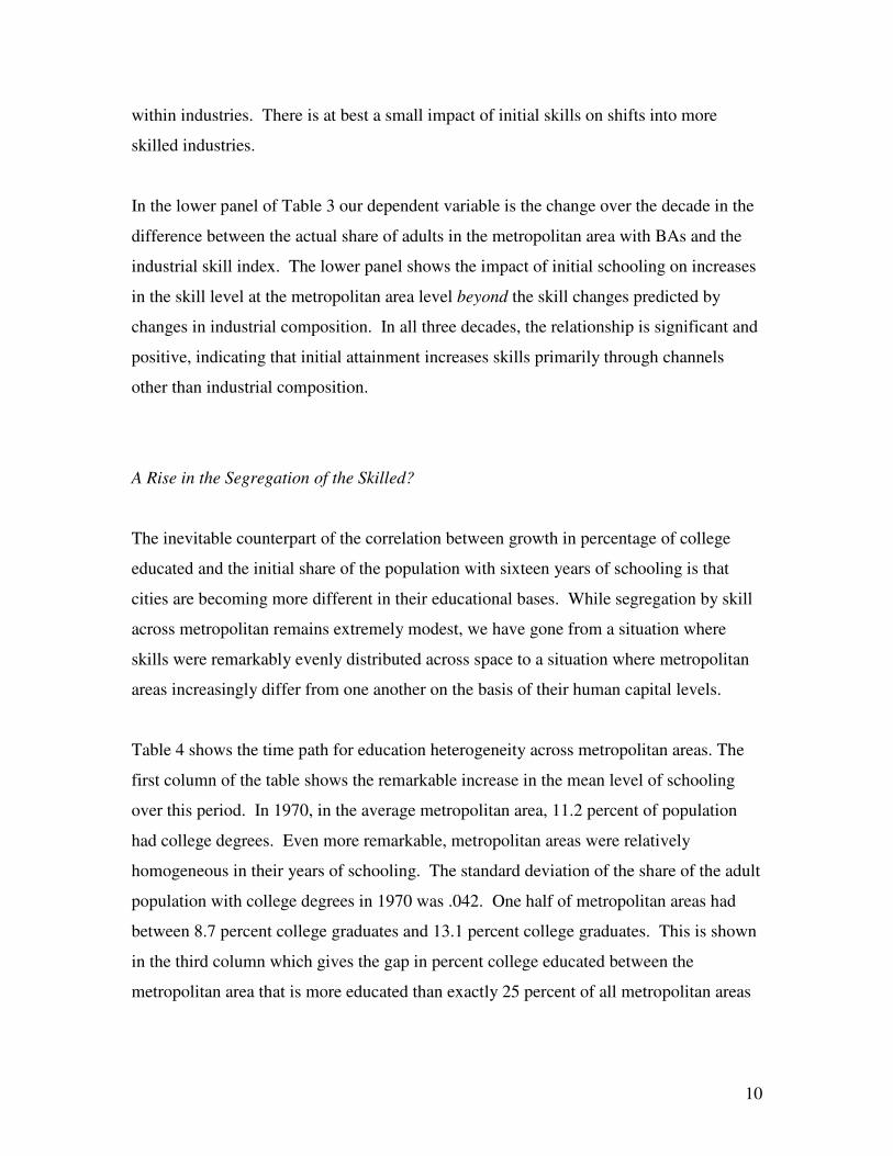
within industries. There is at best a small impact of initial skills on shifts into more

skilled industries.

In the lower panel of Table 3 our dependent variable is the change over the decade in the

difference between the actual share of adults in the metropolitan area with BAs and the

industrial skill index. The lower panel shows the impact of initial schooling on increases

in the skill level at the metropolitan area level beyond the skill changes predicted by

changes in industrial composition. In all three decades, the relationship is significant and

positive, indicating that initial attainment increases skills primarily through channels

other than industrial composition.

A Rise in the Segregation of the Skilled?

The inevitable counterpart of the correlation between growth in percentage of college

educated and the initial share of the population with sixteen years of schooling is that

cities are becoming more different in their educational bases. While segregation by skill

across metropolitan remains extremely modest, we have gone from a situation where

skills were remarkably evenly distributed across space to a situation where metropolitan

areas increasingly differ from one another on the basis of their human capital levels.

Table 4 shows the time path for education heterogeneity across metropolitan areas. The

first column of the table shows the remarkable increase in the mean level of schooling

over this period. In 1970, in the average metropolitan area, 11.2 percent of population

had college degrees. Even more remarkable, metropolitan areas were relatively

homogeneous in their years of schooling. The standard deviation of the share of the adult

population with college degrees in 1970 was .042. One half of metropolitan areas had

between 8.7 percent college graduates and 13.1 percent college graduates. This is shown

in the third column which gives the gap in percent college educated between the

metropolitan area that is more educated than exactly 25 percent of all metropolitan areas

11

and the metropolitan area that is more educated than exactly 75 percent of all

metropolitan areas.

In 1980, the average share of metropolitan areas with college degrees increased to 16.4

percent and the standard deviation rose to .054. The percentage increase in the mean

during this period was much larger than the percentage increase in the standard deviation,

so the coefficient of variation actually fell. Still, this does not lessen the fact that cities

were increasingly differentiating themselves on the basis of years of schooling during this

decade. The gap between 25th percentile and 75th percentile in the share of adults with

college degrees increased to 6.3 percent.

In the 1990s, the mean share of the population with college degrees increased further to

18.7 percent, and the standard deviation of this number across metropolitan areas

increased to .063. In 1990, the mean share of metropolitan area population with college

degrees increase to 22.6 percent and the standard deviation increased to .073. The gap

between the 25th percent and the 75th percentile continued to widen to 9.6 percentage

points. The rising standard deviation reflects the increasing weight in the tails of the

distribution. By 2000, there were 62 metropolitan areas with less than seventeen percent

of their adults had college degrees and 32 where more than thirty-four percent of their

adults had college degrees. Since the distribution is truncated below at zero, the most

impressive growth has been at the upper tail of the distribution. In 1970, no metropolitan

area had more than 30.8 percent of its adult population with college degrees. In 2000,

there were 49 metropolitan areas where more than 30.8 percent of adult population had

sixteen years of schooling or more.

While there is clearly a correlation between change in the share of adults with college

degrees and the initial share of the population that is well educated, and it is clear that the

variance of these shares is rising over time, the changes in the segregation of the skilled

across metropolitan areas remain modest. Also in Table 4, we use standard measures

from the segregation literature to assess the degree to which the skilled are segregated

across metropolitan areas. Our first measure is the dissimilarity index:

12

(6) � −=MSAs

ityDissimilarBAs w.o.Adults Total

BAs w.o.AdultsBAs w.Adults Total

BAs w.Adults21 MSAMSA

where MSABAs w.Adults refers to the number of adults in the metropolitan area with

college degrees, MSABAs w.o.Adults refers to the number of adults in the metropolitan

area without sixteen years of schooling. This measure can be interpreted as the share of

people with sixteen years of schooling who would have to move for there to be a

completely even distribution of people with sixteen years of schooling across all

metropolitan areas.

Table 4 shows the time path of this index. Dissimilarity does rise over this period from

.11 to .128. These numbers are quite low relative to the segregation of other groups such

as African-Americans and they reflect the fact that skills are still distributed relatively

evenly over space. So while skilled people are becoming more segregated, this trend is

mild and the skilled still remain relatively integrated over space.

The second primary measure of segregation is the isolation index or:

(7) � −=MSAs

IsolationAdults Total

BAs w.Adults TotalBAs w.Adults Total

BAs w.AdultsAdults

BAs w.Adults MSA

MSA

MSA

where MSAAdults refers to the number of adults in the MSA and Adults Total refers to the

total number of adults across all metropolitan areas. The first term in the expression

averages across adults with sixteen years of schooling the average share of adults with

sixteen years of schooling in their metropolitan area. The second term subtracts off the

average share of adults with sixteen years of schooling in the sample as a whole. This

index captures the extent to which people with college degrees are surrounded only by

like people.

13

If we didn’t correct for the overall increase in the share of the population with college

degrees then the isolation index would rise from 12.8 percent to 28.2 percent over the

time period. At the start of the time period, on average someone with a college degree

lived in a metropolitan area where about one-eighth of the population had a similar

credential. Thirty years later, a typical person with a college degree lives in a

metropolitan area where more than one-in-four have the same amount of schooling.

But most of this gain reflects the rise in education generally and when we correct by

subtracting the sample wide share of the population with sixteen years of schooling, this

isolation index increases only from .008 to .016. This increase is real but modest and the

average college graduate lives in a metropolitan area that is only slightly better educated

than the average person without a college degree.

III. Sorting by Skills: Theory

In this section, we present a simple model of urban agglomeration which provides an

explanation for the tendency of skilled people to live among other skilled people. The

core assumption in the model is that the number of employers depends on the number of

people, and particularly, the number of skilled people in the area.2 We think of this as

reflecting a process where entrepreneurs come out of a city’s labor force and then tend to

stay generally in that area. Duranton and Puga (2001) present a more thorough

discussion of location decisions of innovators in urban areas.

While we will generally be treating firms as fixed, we assume that workers are mobile

and their utility in the city must be equal to their reservation utility which equals U for

skilled workers and U for unskilled workers. Utility for high skill workers in city “i”

equals: ( )( )Hi

Li

Hi

HHi ANNCWU ,+− ; utility for low skill workers equals

( )( )Li

Li

Hi

LLi ANNCWU ,+− . The variables L

iW and HiW refer to the endogenously

determined wages received in city i by low and high skill workers respectively. The

2 The link between population size and innovations is emphasized by Kremer (1993).

14

variables LiA and H

iA refer to the exogenous amenity levels in the city which can

disproportionately attract high and low skill individuals.

The terms ( )Li

Hi

H NNC + and ( )Li

Hi

L NNC + refer to the cost of living in city i

(primarily housing costs) which is a function of the sum of the total number of high skill

workers ( HiN ) and the total number of low skill workers ( L

iN ), and we denote this N.

We allow an increase in population to have different impacts on the cost of living for

both high and low skilled workers. The equations ( )( ) UANNCWU Hi

Li

Hi

HHi =+− , and

( )( ) UANNCWU Li

Li

Hi

LLi =+− ,, then determine the labor supply into this city. We can

use these two equalities to define implicit functions ( )( )Li

Hi

HHi

Hi NNCAW +, and

( )( )Li

Hi

LLi

Li NNCAW +, which reflect the wages that firms need to pay workers to induce

them to stay in a town of size N.

There are two types of firms each of which employs only one type of worker. Each firm

sells its product at a price of 1 and has access to a production technology: )( jj

i Qfθ

where j equals H or L, jQ refers to the number of workers hired by the firm, and f(.) is

monotonically increasing and concave. Each firm is assumed to be started by an

entrepreneur who receives the excess rents from the firm. The limiting factor to

entrepreneurship is assumed to be new ideas and these ideas occur stochastically in the

population. The number of entrepreneurs whose firms employ high type workers is

assumed to equal Hii Nhh 1φ+ . The term ih is an exogenous constant and the term

HiNh1φ assumes that the amount of entrepreneurship of this type is proportional to the

number of high skilled people living in this community. We are assuming that high skill

workers produce a new idea with probability 1h , and with probability φ this new idea

involves the employment of high skill workers. We also implicitly assume that there is

some natural comparative advantage to this location that ensures that these firms remain

in the area, or that new ideas are location-specific so that they cannot be taken elsewhere.

15

The number of entrepreneurs who open low skill firms equals Hi

Lii NhNll 11 )1( φ−++ .

The term il is again an exogenous constant. The term LiNl1 describes the number of low

skill firms started by low skill entrepreneurs. We assume that unskilled workers cannot

innovate in a way that employs more skilled workers. Finally, the term HiNh1)1( φ−

refers to the number of high skill entrepreneurs who start firms that employ less skilled

workers. The parameter φ is important in the model and captures the extent to which

high skill people come up with ideas that lead only to the employment of high skill

workers.

The assumption that the number of firms is proportional to the number of workers of each

type is the core of the model. This assumption embeds two different ideas. First, we are

assuming that innovations just occur randomly to workers. We are assuming that these

events are sufficiently rare in the life of most workers that they can be treated as being

measure zero in the location decision, but when they occur they create the possibility for

a new product that can produce sizable rents. Second, we are assuming that when a

worker has a new idea, that worker stays in his home area. This fixed nature of

employment can be justified if entrepreneurs want to stay in their cities for consumption

reasons or if the innovation makes use of unique aspects of their own urban environment.

This connection between population size and entrepreneurship is the key agglomeration

effect in this model. Workers are both providers of labor supply and potential innovators

who create labor demand. We have also assumed that unskilled workers only innovate in

firms that employ other unskilled workers, but that when skilled workers innovate with

probability φ they employ their own human capital type and with probability φ−1 they

employ workers of another human capital type. We think it is reasonable to assume that

people without education will have difficulty figuring out a new production process that

uses entirely people with more education, but it is possible that skilled people (like Henry

Ford) will occasionally develop firms that use less skilled workers.

16

With these assumptions the core equations of the model equate the marginal product of

labor for both high skilled firms and low skilled firms with the wage that is demanded by

workers to stay in that town, or ( )( )Li

Hi

HHi

HiH

ii

HiH

i NNCAWNhh

Nf +=��

�

����

�

+′ ,

1φθ and

( )( )Li

Hi

LLi

LiL

iHii

LiL

i NNCAWNlNhl

Nf +=��

�

����

�

+−+′ ,

)1( 11φθ . These equations do not

include any classic human capital externalities (as in Lucas, 1988), and the only benefit

for less skilled workers from living around the more skilled is actually a pecuniary

externality. If 0=ih , the model suggests that each firm has decreasing returns to skilled

workers, but that the city as a whole has constant returns to skilled workers.

Comparative statics then follow:

Proposition 1: The number of skilled people in the city will decline and the number of

unskilled people in the city will rise if Liθ , il or L

iA increase.

If ( )NC L '1 φ−

is sufficiently high, then an increase in Hiθ , il or H

iA will cause both

the number of skilled people and the number of unskilled people in the city to rise.

If ( )NC L '1 φ−

is sufficiently low, then an increase in Hiθ , il or H

iA will cause the

number of skilled people in the city to rise and the number of unskilled people in the city

to fall.

Proposition 1 provides the core results of this model. Parameters that increase the

attractiveness of the city for the less skilled, such as Liθ , il or L

iA , will cause the cost of

living to rise and skilled people leave the city. An increase in Liθ (the productivity of

less skilled firms) or il (the number of firms specializing in less skilled workers) will

create an increase in labor demand for the less skilled in that location. An increase in LiA reflects an amenity that particularly attracts the poor, such as more generous welfare

payments, will also repel the rich as it seems to have done in cases like East St. Louis.

17

The more interesting results concern the comparative statics on Hiθ , ih and H

iA . Because

an increase in the skilled leads to more firms that hire both the skilled and the unskilled it

is quite possible that a parameter that makes a place more attractive to the skilled will end

up attracting more unskilled as well. The impact of the skilled on the location of the

unskilled depends on the magnitude of ( )NC L '1 φ−

. The numerator of this expression

captures the extent to which the skilled are likely to produce innovations that employ the

unskilled. The denominator captures the extent to which an increase in the number of the

skilled living in the area drives up the cost of living for the unskilled.

When ( )NC L '1 φ−

is high, either because the skilled innovate in a way that employs the

unskilled or because ( )NC L ' is low, then we would expect the skilled and unskilled to

live together. Any location specific characteristic that attracts the skilled, such as a

consumption amenity ( HiA ), or the productivity of more skilled workers ( H

iθ ) or an

increase in the number of firms that hire the more skilled, will also attract more unskilled

people as well who will choose to locate near the skilled.

However if ( )NC L '1 φ−

is low, either because the skilled innovate in a way that only

employs the skilled or because ( )NC L ' is high, then the forces that attract the skilled will

tend to push the unskilled away. In this case, the impact of the skilled on the cost of

living overwhelms the impact of the skilled on the employment prospects for the less

skilled. Furthermore, in this scenario we should expect to see more clustering of skilled

and unskilled people in different metropolitan areas.

This proposition suggests two reasons why we should see an increasing tendency for

more skilled workers to go to cities that have advantages for the skilled. First,

innovations of the skilled may now tend to employ primarily skilled persons while in the

18

past, innovative firms founded by skilled people often employed large numbers of

unskilled people. In a sense this is a comparison between Henry Ford and Bill Gates.

Both individuals were themselves skilled, but Ford’s production involved vast numbers

of unskilled workers. Gates’ company primarily employs the more skilled.

A second reason why we should expect to see a change in the locational patterns of the

skilled and unskilled is increasing housing supply inelasticity. When housing supply is

sufficiently elastic so that ( )NC L ' is small, then even if the innovations of the skilled

only rarely employ unskilled, the unskilled will still come to the town because the cost of

living there is so modest. However, when ( )NC L ' is large then the skilled will push up

housing prices for the unskilled by such a large amount that they will not be willing to

pay to live around the skilled entrepreneurs. As such, a second possible reason why the

skilled increasingly locate around each other is that the housing supply has gotten more

inelastic over time, possibly as a result of land use regulations (Glaeser, Gyourko and

Saks, 2005).

We end this section by considering the impact of an increase in φ on wages, but in this

case we hold city populations fixed. A model of the form described above has essentially

perfect labor supply so that shocks to labor demand can only have a limited effect on

nominal wages and no effect on real wages. This could be modified by assuming

heterogeneous tastes for different locales, but this would complicate the situation

excessively. Instead, we simply assume that in some short run, city populations are fixed.

As such, this proposition should be seen as a partial equilibrium analysis that restricts

population movements to changes in φ . If population levels are allowed to move freely

with respect to changes in this parameter, then the differences in wages will be entirely

determined by differences in the cost of living functions and will not reflect different

demand for workers. To simplify matters further, we assume that 0== ii lh and find:

19

Proposition 2: The difference in wages between the skilled and unskilled will increase

with φ .

If higher skill levels in cities are caused by differential amenity levels or higher

levels of Hiθ then as φ rises, the sensitivity of average income to the share of high skilled

people in the area will also rise as long as f’’ is effectively constant in the range of

interest and 21

21

lhL

iH

i θθ > .

If αQQf =)( then the differences in the logarithm of wages between skilled and

unskilled that is associated with an increase in φ will be greater in areas where Li

Hi

NN

is

higher.

Proposition 2 provides the basis for our analysis in Section V where we look at the

changes in wages over time. The proposition has three parts. First, as φ rises this will

mean that there are more firms using skilled labor relative to firms using unskilled labor.

This causes labor demand for skilled workers to rise and this will increase the wages of

the skilled relative to the unskilled. This effect is not surprising, but it relates to the well

known rise in returns to skill over the last 25 years. If new firms make more use of

skilled workers, then this provides one possible reason for this phenomenon.

The second part of the proposition shows that the connection between area level skills

and area level income will increase as φ rises. The primary reason for this is that the

rise in returns to skill naturally means that the relationship between area level skills and

area level income will rise.

The third part of the proposition suggests that an increase in φ will cause greater wage

gaps between skilled and unskilled in more skilled areas. The reason for this is that

higher values of φ mean that the skilled entrepreneurs, who are more abundant in more

skilled cities, generally raise the wages of skilled laborers. A higher value of φ

20

essentially increases the degree of complementarity across skilled people since it means

that skilled people are more likely to end up hiring other skilled people.

IV. Skills, Innovation and Housing Supply

We now turn to evidence on changes in the ratio ( )NC L '1 φ−

. We start by documenting the

tendency of skilled innovators to hire skilled laborers. We then turn to the changes in

housing supply elasticity.

Skills and Innovation

One possible explanation for skill divergence among cities is that the innovations of

skilled entrepreneurs disproportionately utilize skilled workers. Although we are not

aware of a publicly available data source that would allow us to test this hypothesis

directly, we have assembled several pieces of evidence that are broadly consistent with

such an explanation.

Perhaps the most direct evidence on the relative level of human capital in new firms

comes from Abowd et al. (2001), who use a restricted access data set from the Census

Bureau’s Longitudinal Employer-Household Dynamics Program. Examining the Illinois

economy, the authors find that one important factor contributing to the overall increase in

human capital in the 1990s is that entering businesses had substantially more skilled

employees than exiting businesses. They note, however, that upskilling within

continuing businesses accounts for the largest share of the aggregate increase in skills.

This work does not specifically relate to the difference between skilled and unskilled

entrepreneurs, but if we believe that the majority of entrepreneurs are skilled, then this

fact supports our assumption that φ has changed.

Another testable implication of the model is that the pattern of skill divergence we

observe across cities also holds across industries. Using the census PUMS data, we

21

computed average educational attainment by 3-digit industry and examined whether

highly skilled industries have a tendency to become more skilled over time. Column one

of Table 5 shows this relationship. For each time period, there is a positive association

between the initial share of workers with a college degree and the growth in college

attainment over the succeeding decade. The association is only significant at the 10

percent level in the 1980s, however. The relationship between initial attainment and

subsequent upskilling is largest in the 1970s, suggesting that the rate of skill divergence

may have decreased over time. However, we are not able to reject the hypothesis that

skill divergence in the 1990s is equal to that observed in the 1970s.

We next investigate whether employment in more skilled industries is growing over time.

This fact might be understood as testing the hypothesis that skilled people are particularly

innovating in recent time periods. In every decade, we see a positive association

between initial college attainment in an industry and subsequent employment growth in

the industry. This result is simply a re-affirmation of the common finding in the wage

structure literature that between-industry demand shifts have favored college workers

(e.g., Katz and Murphy, 1992). The relationship is strongest in the 1980s, although we

cannot reject that the coefficients for the 1980s and 1970s are equal. We can, however,

reject that the relationship in 1990s is equal to either of the earlier decades, indicating that

the relationship between initial attainment and subsequent employment growth has

declined over time, consistent with Autor, Katz and Krueger (1998). In sum, two patterns

we observed across cities are also evident across industries; namely, the tendency for

highly skilled cities and industries to become more skilled over time and to add more

jobs.

While the above evidence on skill and employment growth across industries is consistent

with the basic hypothesis that skilled entrepreneurs disproportionately hire skilled

workers, we have still not shown an explicit link between the skills of entrepreneurs and

workers. Although we lack data on entrepreneurs specifically, we approach this problem

by computing educational attainment by occupation within industries. Using the census

22

PUMS, we compute the percentage of college graduates in three broad occupational

categories: managerial and proprietary, technical and professional, and all other workers.3

We compute these occupational attainment estimates by 3-digit industry code, excluding

farming and agriculture from the analysis. As shown in Table 6, we then correlate the

educational attainment among managers and owners with the educational levels for the

other groups. In 1970, across industries the correlation between manager’s education

levels and the education level of ordinary workers was 38 percent. In 2000, the

correlation between manager’s education level and the education level of ordinary

workers was 51 percent. This difference is strongly significant statistically.

Figure 3 shows the relationship between the share of managers with college degrees and

the share of ordinary workers with college degrees in 1970. The regression line in the

graph shows that on average a one percent increase in the share of managers with college

degrees is associated with a .15 percent increase in the share of ordinary workers with

college degrees. Figure 4 shows the same relationship for 2000. The regression line in

that growth shows that on average a one percent increase in the share of managers with

college degrees in 2000 is associated with a .38 percent increase in the share of ordinary

workers with college degrees. In other words, high skill managers increasingly manage

firms with high skill workers.

In Table 6, we also show the correlations between the education of managers and the

education of professional and technical workers. This correlation coefficient was .42 in

1970 and .64 in 2000. Again, the change is statistically significant. Highly skilled

managers and skilled technical workers have also increasingly concentrated within

industries.

3 Specifically, using the PUMS occupation codes (Ruggles et al. 2004), we classify individuals into three categories: Managers, Officials, and Proprietors (codes 200 to 290); Professional and Technical (codes 000 to 099); and all other workers. We exclude farming occupations (codes 100, 123, and 810 to 840) and those with missing values from the analysis.

23

Our findings are not definitive and there are substantial questions about causality in all of

our empirical findings, but our evidence suggests the idea that skilled entrepreneurs and

managers disproportionately hire skilled labor to be a promising explanation for skill

divergence across cities. The increasing correlation between managerial and worker

skill, and the persistent tendency for initial skilled industries to become more skilled over

time provides some evidence for this view. These results are also broadly consistent with

Kremer and Maskin’s (1996) finding of increasing segregation of high- and low-skill

workers into separate firms.

Housing Supply

A second possible explanation for the increasing tendency of skilled cities to become

more skilled is that housing supply appears to have become more inelastic. While we

lack compelling measures of supply elasticity, there are a variety of pieces of evidence

that do point toward an increasing inability to build more housing cheaply. In this

section, we summarize that evidence.

The first piece of evidence pointing toward this inelasticity is the increasing gap between

housing prices and construction costs. In 1970, in almost every metropolitan area, most

houses were valued at less than 1.25 times construction costs. Ninety percent of the areas

in a 102 metropolitan area sample had an average price that was less than twelve percent

more than construction cost. Thirty years later in the average metropolitan area, housing

prices cost more than 46 percent more than construction costs (Glaeser, Gyourko and

Saks, 2005). These prices must reflect increasing difficulties of building readily.

A second piece of evidence suggesting declining housing supply elasticity is the

declining number of new homes that are being built, particularly in high cost areas. In a

sample of homes in 102 metropolitan areas, the median metropolitan area in 1970 built

35 percent of its homes over the previous decade. In 2000, the median metropolitan area

built only 14 percent of its homes over the previous decade (Glaeser, Gyourko and Saks,

24

2005). Detailed analysis of particular metropolitan areas shows a stunning decline in

permitting between 1960 and today (Glaeser, Gyourko and Saks, 2004).

A third piece of evidence showing declining elasticity is that the connection between

housing prices and new construction is falling. Glaeser, Gyourko and Saks (2004) show

that in the 1960s and 1970s in New York City, new construction increases when housing

prices rise. In the 1990s, this correlation disappears. Glaeser, Gyourko and Saks (2005)

find across metropolitan areas that higher housing prices are becoming more negatively

associated with new construction over time. This decline is consistent with an increasing

inability to build in high cost regions.

But while there is evidence suggesting that housing supply has become more inelastic

over time, there is little evidence suggesting that the housing price premium associated

with living in a better educated city has increased. If we regress median housing values

in 1980 on the share of adults with bachelor’s degrees during that year, we estimate:

(8) ( ) 1980)241(.)042(.1980 012.322.10 CollegeValueLog •+=

Standard errors are in parentheses and there are 318 observations. The r-squared is 33

percent. Data are from the census and housing values are in 2000 dollars.

The same regression in 2000 yields:

(9) ( ) 2000)207(.)051(.2000 007.388.10 CollegeValueLog •+=

There are 318 observations and the r-squared is 40 percent. Data are from the census.

There has been a tendency of housing prices to rise in highly educated areas, but

generally the price increase has been lower than the price increase that would be

suggested by rising wages in those areas (Glaeser and Saiz, 2004).

25

A second piece of evidence suggesting that high housing prices are not driving the

increasing tendency of the skilled to move toward skilled areas is that controlling for

lagged housing prices does little to change to relationship between initial skill levels and

the growth in the share of the population with at least sixteen years of schooling. For

example if we modify our basic regression from Table 1 to include the lagged median

housing value, we estimate:

(10) )(001.139.004. 1990)002(.1990)014(.)02(.19902000 ValueLogCollegeCollegeCollege •+•+−=−

where )( 1990ValueLog refers to the logarithm of median housing value in the metropolitan

area in 1990. The r-squared in this regression is 28 percent and there are 318

observations. The coefficient on share with sixteen years of schooling or more is

essentially unchanged from that reported in Table 1, regression 1. The coefficient on the

lagged median housing value is essentially zero. There is no sense that controlling for

lagged housing prices impacts the relationship between initial share of the adult

population with sixteen years of schooling or more and later growth in that variable.

Overall, there is little evidence supporting the idea that increasing inelastic housing can

explain the divergence of human capital levels. While housing supply is becoming more

inelastic, there has been a substantially higher cost associated with living in educated

metropolitan areas for many decades. As a result, it doesn’t seem likely that high

housing prices are the main reason for the increasing tendency of the skilled to live in

more skilled areas.

V. Evidence on Income Patterns across Metropolitan Areas

Finally, we turn to the implications of skill agglomerations for wages and income

patterns. First we turn to the correlations between area level skills and area level income.

Second, we turn to patterns of metropolitan area income convergence.

26

Income and Education across Metropolitan Areas

The model suggested that if the tendency of skilled entrepreneurs to employ skilled

laborers is rising, we should expect an increasing correlation between area level skills and

area level income. Indeed, the correlation between education and income is also

increasing. Figure 5 shows the relationship between the percent of the population with a

college degree and the logarithm of per capita income at the metropolitan area level in

2000. The income data come from REIS and educational attainment from the census.

The regression line shown in the figure is:

(11) ( ) 2000)11(.)02(.2000 63.18.9 CollegeIncomeLog •+=

The r-squared of this regression is 40 percent and there are 318 observations. In 1970,

the relationship is much weaker as shown in Figure 6. The regression line in this case is:

(12) ( ) 1970)21(.)02(.1970 84.01.8 CollegeIncomeLog •+=

There are again 318 observations and the r-squared is 4.6 percent. The correlation

between the logarithm of mean income in the metropolitan area and the percent of the

population with college degrees increases from 21.4 percent in 1970 to 32.2 percent in

1980 to 49.8 percent in 1990 to 63.3 percent in 2000.

While these trends are impressive, these results in no sense correct for the general rise in

returns to skill. To do this, we follow Rauch (1993) and turn to individual level

regressions where we examine the changing correlation between metropolitan area level

skills and wages holding individual skills constant. Our basic specification is:

(13) ControlsOtherSchoolingSchoolingWageLog tMSAttittMSAi +•+•= ,,,, )( βα

27

Data are from the PUMS (Ruggles et al. 2004).4 For each individual, the logarithm of

hourly income for individual i at time t living in a particular metropolitan area

( )( ,, tMSAiWageLog ) is regressed on their own education and the percentage of adults with

a college degree in the metropolitan area ( tMSASchooling , ). The coefficients on both

individual schooling and metropolitan area level schooling are allowed to change over

time. We estimate the individual schooling effects by including dummy variables for

individual years of education. We include only males between 25 and 55 with complete

observations. We control for race using dummy variables and for age by using a fourth

order polynomial. The coefficients are also allowed to change over time.

In all of our regressions, we use average schooling in 1970 as our measure of

metropolitan area schooling and estimate its effect on individual wages in 1980, 1990,

and 2000. This has the effect of limiting the endogeneity of our key independent variable

and of focusing on the wage effects of initially high skilled cities. If we used

contemporaneous schooling levels, then the correlation with wages is almost sure to be

the result of omitted variables that both raise demand for high skilled workers in the

region and later attract more skilled people into that region.

The results are shown in Table 7. The first equation shows our basic results, which echo

those of Rauch (1993) and Glaeser and Saiz (2004). There is a strong basic connection

between the share of college graduates in the metropolitan area and the logarithm of the

hourly wage. Each extra percent of adults with a college degree is associated with .58 log

points of extra income in 1980. This effect rises over time and in 2000, each extra

percent of metropolitan area college attainment is associated with 1.22 log points of extra

income. The f-tests reported in the bottom row of the table confirm that this change is

statistically significant.

Perhaps the most significant issue with this Rauch (1993) type regression is the

possibility that metropolitan area schooling is correlated with unobserved individual

4 For each PUMS year, we use the sample with the richest metropolitan area coverage, which is the 1 percent sample in 1970, 1980, and 1990, and the 5 percent sample in 2000 (Ruggles at al. 2004).

28

human capital. After all, since more skilled metropolitan areas are defined on the basis of

people with more observed human capital sorting into them, it would not be surprising

that people with more unobserved human capital also sort into them. If we are willing to

accept that this sorting has not changed over time and that the coefficient on unobserved

ability is not changing over time (both of which are quite debatable assumptions), then

controlling for metropolitan area fixed effects is one way of addressing the problems

related to unobserved ability sorting.

In regression (2) of Table 7, we repeat our basic specification including metropolitan area

fixed effects. As such, we can no longer estimate a baseline relationship between

metropolitan area years of schooling and the logarithm of hourly wages. However, we

can estimate the extent to which metropolitan area schooling has become a more

important predictor over time by looking at the interaction between metropolitan area

schooling in 1970 and dummy variables for the years 1990 and 2000. Again, the

regression shows a significant increase in the correlation between MSA level education

and individual wages. The coefficient on education rises by .51 between 1980 and 1990

and .16 between 1990 and 2000. Including MSA fixed effects does little to change the

basic relationships identified in regression (1).

In regressions (3)-(5), we reproduce regression (1) of Table 7 for different education

subgroups (results including MSA fixed effects are quite similar). In this case, we are

looking at whether there has been a change in the correlation between metropolitan area

education and wages for different subgroups and this represents a test of the prediction of

proposition 2 that an increase in the parameter φ , which represents the tendency of high

human capital entrepreneurs to hire their own, will lead to higher wages particularly for

high skilled workers. We divide the population into people with 16 years of education or

more, between 12 and 16 years of education and strictly less than 12 years of education.

This follows the work of Mare (1995) who identified different Rauch (1993) effects

among education subgroups.

29

In regression (3), we see the changing impact of area-level education on high school

dropouts. The effect only gets slightly stronger over time. The coefficient rises from .75

to 1.15, and we cannot reject that the coefficients for 1980 and 2000 are equal. In

regression (4), we report results for high school graduates and those with some college.

In this case, the basic effect is stronger and the coefficient rises between 1980 and 2000

from .45 to 1.08. For this group, all of the increase appears to have come between 1980

and 1990, as we cannot reject that the coefficients for 1990 and 2000 are equal. In

regression (5), we report results for college graduates and in this case the coefficient rises

from .68 to 1.41. The correlation between area level education and individual wages is

about even for college graduates and for high school dropouts in 1970, but by 2000 a gap

emerges in which the highly skilled benefit most from being around other skilled

workers.

These regressions treat metropolitan area level schooling as exogenous, which may not

be appropriate. After all, the major theme of the paper is the sorting of skilled people

into more skilled areas. Thus, we prefer to see these empirical results as tests of one

implication of the model rather than as estimates of a meaningful economic parameter.

The End of Regional Convergence?

In this final empirical section, we present what may be one of the most interesting

consequences of increased sorting by skill: the decline of metropolitan area convergence.

The basic convergence regression is:

(14) ( ) ControlsOther IncomeMSA IncomeMSA IncomeMSA

1-t1-t

t +•+=���

����

�LogLog βα

This regression is known to be biased downwards if there is time varying measurement

error in metropolitan area income. A significant literature (e.g. Barro and Sala-i-Martin,

1992) has documented a general pattern of regional convergence, and also reports a

decline in the amount of convergence in the 1980s relative to earlier time periods.

30

In Table 8, we estimate these convergence patterns for the 1970s, 1980s and 1990s using

two different measures of income: average wage and per capita income, both from REIS.

In the Table 8a, we include only initial income as a regressor. Both measures of income

data show the same pattern. There was substantial convergence in the 1970s which

decreased over time. In the case of the wage data, shown in regressions (1)-(3), the

coefficient on initial income is -.06 in the 1970s and .02 in the 1990s. These coefficients

move from being significantly negative to being significantly positive. Figure 7 shows

wage convergence in the 1970s; Figure 8 shows wage divergence in the 1990s.

Regression (4)-(6) of Table 8a show the results for income. In this case, convergence in

the 1970s is even more striking and the basic coefficient is -.11. In the 1990s, the

coefficient estimate is positive but not statistically significant. The change in coefficients

for income is even larger than the change in coefficients for wages. In the 1970s, poorer

metropolitan areas were getting richer relative to richer metropolitan areas. In the 1990s,

richer areas got richer relative to poorer areas.5

One potential explanation for this fact is the rise in returns to skill and the increased

sorting across metropolitan areas. In the Table 8b, we repeat our convergence

regressions controlling for the change in the share of the adult population with college

degrees in the metropolitan area. This control eliminates all signs of divergence. When

we use log of wages in the first three regressions there is still a substantial decline in the

level of convergence over the past 30 years. When we use log of income in the last three

regressions, the change in the amount of convergence is more modest and it does appear

that controlling for the change in the share of the population with college degrees

explains the decline in regional convergence.

Convergence has declined substantially over the last 30 years. One potential reason for

this is that initial high income, and high skill, places are increasingly attracting more

5 Barro and Sali-i-Martin (1999) find that convergence in personal income across U.S. states appeared to end in the 1980s, a result which they attribute to oil shocks. They do not report results for the 1990s.

31

skilled people. When we control for the changes in the skill composition at the area

level, convergence reappears although there still seems to be some change between the

1970s and the 1990s.

VI. Conclusion

In this paper, we have documented that places with higher levels of human capital have

attracted more skilled people over the last three decades. The correlation between the

initial share of metropolitan area adults with college degrees and change in that variable

over the 1990s is enormously strong. Educated people are still remarkably spread out

across areas, but it is possible that segregation by skill might become more significant

over time if this trend continues.

One potential explanation for this phenomenon is that labor demand is often created by

local entrepreneurs who start firms in their own city. If skilled people are increasingly

likely to start firms that hire other skilled people, then this could readily explain why an

initially high level of skills would lead to a growth in the skill composition of a city over

time. The initial population starts new firms and hires new skilled people. According to

this view, the key change over the last 30 years is that high skill entrepreneurs

increasingly innovate in ways that lead to more employment for other skilled people.

There is some evidence that such a change has occurred. The correlation between the

skill level managers and workers within industries has been rising over time. The wages

for skilled workers in skilled cities have been rising relative to the wages of unskilled

workers in the same cities. This is a prediction of a model where the skill level in a place

leads to an increase in labor demand particularly for skilled workers.

While it seems that the tendency of the skilled to move to skilled areas is partly

responsible for the remarkable decline in income convergence across metropolitan areas,

it is not obvious that a public policy response to this change is needed or appropriate.

After all, basic results in welfare economics tell us that while wealth differences across

32

people may be important, wealth differences across places are not necessarily troubling.

Unless we are confident that the increasing tendency of skilled cities to become more

skilled creates negative externalities for the unskilled, these results suggest interesting

changes across America’s cities but they do not suggest any definite policy action.

33

References

Abowd, J., Haltiwanger, J., Lane, J. and K. Sandusky (2001) “Within and Between Firm Changes in Human Capital, Technology, and Productivity” U.S. Census Bureau, LEHD Program, Technical Paper No. TP-2001-03.

Autor, D., Katz, L. and A. Krueger (1998) “Computing Inequality: Have Computers Changed the Labor Market?” Quarterly Journal of Economics 113(4): 1169-1213.

Barro, R. and X. Sala-i-Martin (1992) “Convergence” Journal of Political Economy 100(2): 223-251.

Barro, R. and X. Sala-i-Martin (1999) Economic Growth, Cambridge, MA: MIT Press. Duranton, G. and D. Puga (2001) “Nursery Cities: Urban Diversity, Process Innovation

and the Life Cycle of Products” American Economic Review 91(5): 1454-1477. Glaeser, E, Gyourko, J. and R. Saks (2005) “Why Have Housing Prices Gone Up?”

American Economic Review, forthcoming Glaeser, E., Gyourko, J. and R. Saks (2004) “Why in Manhattan So Expensive?” Journal

of Law and Economics, forthcoming. Glaeser, E. and A. Saiz (2004) “The Rise of the Skilled City,” Brookings-Wharton

Papers on Urban Affairs: 47-94. Glaeser, E., Scheinkman, J. and A. Shleifer (1995) “Economic Growth in a Cross-Section

of Cities,” Journal of Monetary Economics 36: 117-143. Katz, L. and K. Murphy (1992) “Changes in Relative Wages, 1963-1987: Supply and

Demand Factors” Quarterly Journal of Economics 107(1): 35-78. Kremer, M. (1993) “Population Growth and Technological Change: One Million B.C. to

1990” Quarterly Journal of Economics 108(3): 681-716. Kremer, M. and E. Maskin (1996) “Wage Inequality and Segregation by Skill” NBER

Working Paper # 5718. Lucas, R. (1988) “On the Mechanics of Economic Development” Journal of Monetary

Economics 22: 3-42. Mare, D. (1995) “Living With Graduates” Harvard University Mimeograph. Moretti, E. (2004) “Estimating the Social Returns to Higher Education: Evidence from

Cross-Sectional and Logitudinal Data” Journal of Econometrics 121(1-20: 175-212. Rauch, J. (1993) “Productivity Gains from Geographic Concentration of Human Capital:

Evidence from the Cities,” Journal of Urban Economics 34: 380-400. Ruggles, S., Sobek, M., Alexander, T., Fitch, C., Goeken, R., Kelly Hall, P., King, M.

and C. Ronnander (2004) Integrated Public Use Microdata Series: Version 3.0 [Machine-readable database]. Minneapolis, MN: Minnesota Population Center [producer and distributor].

34

Table 1 -

1990-2000 1980-1990 1970-1980

Change in percentage of adults with bachelor’s

degree

Change in percentage of adults with bachelor’s

degree

Change in percentage of adults with bachelor’s

degree

(1) (2) (3) (4) (5) (6)

Share with bachelor's degree (age 25+) at t-10 0.1376090 0.1173534 0.1296989 0.1472086 0.2433141 0.2050632 (0.0124199) (0.0144661) (0.0147455) (0.0136836) (0.0180609) (0.0199073) Log of population at t-10 0.0004802 0.0053672 0.0030759 (0.0008472) (0.0007268) (0.0008470) Share of workers in manufacturing at t-10 0.0278880 0.0183154 -0.0222402 0.0116913 (0.0086370) (0.0086630) Log of per capita income at t-10 0.02515 0.0046874 0.0117082 (0.0059294) (0.0050577) (0.0060210) Regional fixed effects No Yes No Yes No Yes Observations 318 318 318 318 318 318 R squared 0.2798 0.4001 0.1967 0.516 0.3648 0.4477

Standard errors in parentheses. Observations include all 318 metropolitan statistical areas and primary metropolitan statistical areas (NECMA definitions in

New England). All data are from the 1970, 1980, 1990 and 2000 US censuses. County level data from each census are aggregated to a consistent set of metropolitan area boundaries as defined by the Office of Management and Budget in 1999.

35

Table 2 -

1990-2000 1980-1990 1970-1980

Log change in number of adults with

college degree

Log change in number of adults w.o.

college degree

Log change in number of adults with

college degree

Log change in number of adults w.o.

college degree

Log change in number of adults with

college degree

Log change in number of adults w.o.

college degree

(1) (2) (3) (4) (5) (6)

Share with bachelor's degree (age 25+) at t-10 0.1920509 0.0671524 0.3119436 0.3057507 0.0552201 0.5958813 (0.1019708) (0.0824342) (0.1387881) (0.1258663) (0.2062770) (0.1961645) Observations 318 318 318 318 318 318 R squared 0.0111 0.0021 0.0157 0.0183 0.0002 0.0284 Constant 0.2768968 0.0794055 0.3337489 0.1051539 0.6430823 0.1269587 Test: coefficient for adults with college degree equals coefficient for adults w.o. college degree

Chi squared statistic p-value

2.95 0.086

0.00 0.945

18.93 0.0000

Standard errors in parentheses. Observations include all 318 metropolitan statistical areas and primary metropolitan statistical areas (NECMA definitions in

New England). All data are from the 1970, 1980, 1990 and 2000 US censuses. County level data from each census are aggregated to a consistent set of metropolitan area boundaries as defined by the Office of Management and Budget in 1999.

36

Table 3: 1970s 1980s 1990s Dependent Variable: Change in Industrial Skill Index

Initial share of BAs .0346519 (.0086341)

-.0038652 (.007843)

.0031569 (.008467)

Observations 318 318 318 R squared 0.0485 0.0008 0.0004 Constant .0701384 .0313898 .0315159

Dependent Variable: Change in MSA Education minus Industrial Skill Index

Initial share of BAs .2086622 (.0184751)

.1335641 (.0159062)

.1344521 (.0142837)

Observations 318 318 318 R squared 0.2876 0.1824 0.2190 Constant -.0451122 -.0190977 -.0215653

Standard errors in parentheses.

Observations include all 318 metropolitan statistical areas and primary metropolitan statistical areas (NECMA definitions in New England). Share of BAs is obtained from the US census. County level data from each census are aggregated to a consistent set of metropolitan area boundaries as defined by the Office of Management and Budget in 1999. The Industrial Skill Index is based on data from the Regional Economic Information System (REIS) of the Bureau of Economic Analysis and the public use micro-samples (PUMS) of the U.S. Census, as defined in the text.

37

Table 4: Segregation by Skill

Year Mean share

BAs across

Metropolitan

Areas

Standard

Deviation

25-75

Difference

Dissimilarity

Index

Isolation

Index

1970

.112 .042 .045 .110 .008

1980

.164 .054 .063 .114 .011

1990

.187 .063

.077 .123 .013

2000

.226 .073 .096 .128 .016

Observations include all 318 metropolitan statistical areas and primary metropolitan statistical areas (NECMA definitions in New England). All data are from the 1970, 1980, 1990 and 2000 US censuses. County level data from each census are aggregated to a consistent set of metropolitan area boundaries as defined by the Office of Management and Budget in 1999. Formulas for the dissimilarity and isolation indices are given in the text.

38

Table 5

1970s 1980s 1990s Dependent Variable: Change in Percent BAs in Industry

Initial Share of BAs in Industry .1111996 (.0255809)

.0370845 (.0209052)

.063308 (.0245295)

Observations 142 142 133 R squared 0.1189 0.0220 0.0484 Constant .0467842 .0238306 .0132863

Dependent Variable: Log Change in Industry Employment

Initial Share of BAs in Industry 1.13637 (.2095189)

1.481435 (.2222994)

.4701833 (.2243097)

Observations 142 142 133 R squared 0.1452 0.2445 0.0255 Constant .0485614 -.0937727 -.0812391

Standard errors in parentheses. Data are from the 1970, 1980, 1990, and 2000 PUMS. Educational attainment and total employment are computed for a consistent set of three-digit industry codes, using the PUMS variable ind1950 (Ruggles et al. 2004). Each observation is one three-digit industry.

39

Table 6: Changing Correlation between Education of Managers and Workers Worker BA

Attainment Tech./Prof. BA Attainment

Manager/Proprietor BA Attainment

1970 Worker BA Attainment

1.0000

Tech./Prof. BA Attainment

0.3508 1.0000

Manager/Proprietor BA Attainment

0.3846 0.4246 1.0000

2000 Worker BA Attainment

1.0000

Tech./Prof. BA Attainment

0.5035 1.0000

Manager/Proprietor BA Attainment

0.5147 0.6367 1.0000

Data are from the 1970 and 2000 PUMS (Ruggles et al. 2004). Workers are classified into one of the three occupational categories as described in the text, using the PUMS variable occ1950. Educational attainment is computed by occupational category within three-digit industry codes, using the PUMS variable ind1950. Each observation is a three-digit industry x occupational category.

40

Table 7: IPUMS Estimates of Effects of MSA-Level Education on Individual Wages

Total Sample Total Sample Did Not Graduate High School

High School Graduates, No BA

College Graduates

(1) (2) (3) (4) (5) 1970 Pct BAs x 1980 dummy

.5771157 (.2619824)

Omitted .7529274 (.372206)

.453735 (.2762018)

.6831703 (.2781051)

1970 Pct BAs x 1990 dummy

1.130842 (.2550705)

.5123142 (.0548032)

1.308788 (.3094018)

1.180671 (.2745616)

.9964586 (.2645873)

1970 Pct BAs x 2000 dummy

1.219518 (.2147136)

.6692932 (.0428129)

1.151335 (.2275083)

1.080403 (.2104377)

1.414034 (.2699609)

MSA fixed effects No Yes No No No R-squared .1919 .2092 .0816 .0991 .0967 Observations 2938321 2938321 347696 1681883 908742 F test: 2000=1980 0.0033 0.0000 0.2190 0.0068 0.0081 F test: 2000=1990 0.4743 0.0001 0.4505 0.4805 0.0065 F test: 1990=1980 0.0102 0.0000 0.1091 0.0027 0.1199

Note: Robust standard errors clustered by MSA in parentheses. Data are from the 1970, 1980, 1990, and 2000 PUMS. Regressions include year fixed effects and controls for age up to a 4th degree polynomial, race, Hispanic status, and individual education. All controls are allowed to vary by year. Total sample includes all males aged 25 to 55 who worked at least 10 hours per week. Individuals with missing or imputed values for any of the variables are excluded. The dependent variable is the logarithm of the individual’s hourly wage.

41

Table 8a: Trends in Regional Convergence Log Change in

Wages, 1970-80 Log Change in

Wages, 1980-90 Log Change in Wages, 1990-

2000

Log Change in Income, 1970-

80

Log Change in Income, 1980-

90

Log Change in Income, 1990-

2000 (1) (2) (3) (4) (5) (6)

-0.060 0.025 0.019 -0.114 -0.062 0.014 Initial Log Wages/Income (0.009) (0.010) (0.007) (0.022) (0.030) (0.020) Constant 1.798 0.303 0.254 1.876 1.195 0.265 (0.116) (0.140) (0.102) (0.182) (0.276) (0.198) Observations 318 318 318 318 318 318 R-squared 0.13 0.02 0.02 0.08 0.01 0.00 Standard errors in parentheses Table 8b Log Change in

Wages, 1970-80

Log Change in Wages, 1980-

90

Log Change in Wages, 1990-

2000

Log Change in Income, 1970-

80

Log Change in Income, 1980-

90

Log Change in Income, 1990-

2000 (1) (2) (3) (4) (5) (6)

-0.074 -0.023 -0.001 -0.150 -0.201 -0.090 Initial Log Wage/Income (0.008) (0.010) (0.006) (0.023) (0.022) (4.51)

3.841 6.939 4.230 0.985 4.188 2.250 Change in Share of Adults with College Degree

(0.591) (0.707) (0.463) (0.225) (0.226) (10.51)

Constant 1.780 0.754 0.392 2.117 2.327 1.202 (0.109) (0.131) (0.092) (0.186) (0.201) (6.24) Observations 318 318 318 318 318 318 R-squared 0.23 0.25 0.23 0.13 0.53 0.26 Standard errors in parentheses Observations include all 318 metropolitan statistical areas and primary metropolitan statistical areas (NECMA definitions in New England), using constant 1999 boundaries. Income and wage data are from REIS. Educational attainment is from the census.

42

Figure 1

0.0

5.1

Cha

nge

in P

erce

nt w

ith B

A 1

990-

2000

.1 .2 .3 .4 .5Percent of Adults with BA Degree in 1990

Figure 2

0.0

2.0

4.0

6.0

8.1

Cha

nge

in P

erce

nt w

ith B

A 1

980-

1990

.1 .2 .3 .4Percent of Adults with BA Degree in 1980

Note for Figures 1 and 2: Observations include all 318 metropolitan statistical areas and primary metropolitan statistical areas (NECMA definitions in New England), using constant 1999 boundaries. Data are from the census.

43

Figure 3

0.1

.2.3

.4S

hare

of N

on-T

echn

ical

Wor

kers

w B

A in

197

0

0 .2 .4 .6 .8Share of Managers w BA in 1970

Figure 4

0.2

.4.6

Sha

re o

f Non

-Tec

hnic

al W

orke

rs w

BA

in 2

000

0 .2 .4 .6 .8Share of Managers w BA in 2000

Note for Figures 3 and 4: Data are from the PUMS. Each circle represents one 3-digit industry. Managers and non-technical workers are defined as described in the text.

44

Figure 5

9.5

1010

.511

Log

of P

er C

apita

Per

sona

l Inc

ome

in 2

000

.1 .2 .3 .4 .5Share of Adults with BA Degree in 2000

Figure 6

7.5

88.

59

Log

of P

er C

apita

Per

sona

l Inc

ome

in 1

970

.05 .1 .15 .2 .25 .3Share of Adults with BA Degree in 1970

Note for Figures 5 and 6: Observations include all 318 metropolitan statistical areas and primary metropolitan statistical areas (NECMA definitions in New England), using constant 1999 boundaries. Income data are from REIS and educational attainment from the census.

45

Figure 7

.6.8

11.

21.

41.

6Lo

g C

hang

e in

Avg

Wag

e 19

70-8

0

10 12 14 16 18Average Wage in 1970

Figure 8

.2.4

.6.8

11.

2Lo

g C

hang

e in

Avg

Wag

e 19

90-2

000

12 14 16 18 20Average Wage in 1990

Note for Figures 7 and 8: Observations include all 318 metropolitan statistical areas and primary metropolitan statistical areas (NECMA definitions in New England), using constant 1999 boundaries. Data are from REIS.

46

Appendix: Proofs of Propositions

Proof of Proposition 1: Differentiating equations ( )( ) UANNCWU Hi

Li

Hi

HHi =+− , and

( )( ) UANNCWU Li

Li

Hi

LLi =+− ,, gives us that 1=

∂∂

=∂∂

H

Hi

L

Li

CW

CW

, 01

2 <−=∂∂

UU

AW

Li

Li ,

01

2 <−=∂∂

UU

AW

Hi

Hi .

For any exogenous parameter “x” that enters directly into the equation

( )( )Li

Hi

LLi

LiL

iHii

LiL

i NNCAWNlNhl

Nf +=��

�

����

�

+−+′ ,

)1( 11φθ but not into the equation

( )( )Li

Hi

HHi

HiH

ii

HiH

i NNCAWNhh

Nf +=��

�

����

�

+′ ,

1φθ it follows that:

( )( )

( ) ( ) xN

NCNhh

hQfNC

xN L

i

H

Hii

iHH

i

HHi

∂∂

′++

′′−

′−=∂

∂

2

1φθ

, and since( )

( )( ) ( )

10

2

1

−>′+

+

′′−

′−>NC

Nhh

hQfNC

H

Hii

iHH

i

H

φθ

then x

Nx

N Hi

Li

∂∂

>∂

∂ with opposite sign.

For Lix θ= , differentiation yields

( )( )

( )( ) ��

�

����

�

∂∂

+∂∂′+

+−+

∂∂

−−∂∂

−+′′−=��

�

����

�

+−+′

Li

Li

Li

HiL

Li

Hii

Li

HiL

iLi

LiH

ii

LL

iLi

Hii

Li

NNNC

NlNhl

NNh

NNhl

QfNlNhl

Nf

θθ

φθ

φθ

φθ

φ 2

11

11

11 )1(

)1()1(

)1(

Assume Li

Li

Li

Hi NN

θθ ∂∂

≥≥∂∂

0 , and in that case both terms on the right side of the equation

are non-positive and there is a contradiction so L

i

Hi

Li

Li NN

θθ ∂∂

>>∂∂

0 .

47

For ilx = ,

( ) ( ) ( )

( )( )

( )2

11

11

2

11

)1(

)1()1(

')1(

Li

Hii

i

HiL

ii

LiH

ii

LL

i

i

Li

i

HiL

Li

Hii

Li

LL

i

NlNhl

lN

Nhl

NNhl

Qf

lN

lN

NCNlNhl

NQf

+−+

∂∂

−−∂

∂−+

′′−

���

����

�

∂∂

+∂

∂=

+−+′′−

φ

φφθ

φθ

. If we

assume that i

Li

i

Hi

lN

lN

∂∂

≥≥∂

∂0 , the right hand side of the equation is non-positive and

there is a contradiction so this proves that i

Hi

i

Li

lN

lN

∂∂

>>∂

∂0 .

For LiAx = ,

( )( )

( )( ) ��

�

����

�

∂∂

+∂∂

+

+−+

∂∂

−−∂∂

−+′′−=

∂∂

−

Li

Li

Li

HiL

Li

Hii

Li

HiL

iLi

LiH

ii

LL

iLi

Li

AN

AN

NC

NlNhl

AN

NhAN

NhlQf

AW

'

)1(

)1()1(

2

11

11

φ

φφθ

and again

if we assume that Li

Li

Li

Hi

AN

AN

∂∂

≥≥∂∂

0 , the right hand side of the equation is non-positive

and there is a contradiction so Li

Hi

Li

Li

AN

AN

∂∂

>>∂∂

0 .

For any exogenous parameter “x”, that enters directly into the equation

( )( )Li

Hi

HHi

HiH

ii

HiH

i NNCAWNhh

Nf +=��

�

����

�

+′ ,

1φθ but not into the equation

( )( )Li

Hi

LLi

LiL

iHii

LiL

i NNCAWNlNhl

Nf +=��

�

����

�

+−+′ ,

)1( 11φθ , it follows that:

48

( ) ( ) ( )

( ) ( ) ( ) xN

NCNlNhl

NhlQf

NCNlNhl

NhQf

xN H

i

L

Li

Hii

Hii

LL

i

L

Li

Hii

Li

LL

iLi

∂∂

++−+

−+′′−

−+−+

−′′−

=∂

∂

')1(

)1(

')1(

)1(

2

11

1

2

11

1

φφθ

φφθ

. The denominator of this

expression is always positive. The numerator is positive if and only if

( )( )

( ) LiL

Li

Li

Hii

L NhQfNlNhl

NC 1

2

11)1('

1′′−

+−+>−

θφφ

, which since ( )

( ) LiL

Li

Li

Hii

NhQfNlNhl

1

2

11)1(′′−

+−+θ

φ is a

positive finite number will always hold if ( )NC L '1 φ−

is sufficiently high and will never hold

if ( )NC L '1 φ−

is sufficiently low. If ( )( )

( ) LiL

Li

Li

Hii

L NhQfNlNhl

NC 1

2

11)1('

1′′−

+−+>−

θφφ

, then the signs of

xN L

i

∂∂

and x

N Hi

∂∂

must be the same and if ( )( )

( ) LiL

Li

Li

Hii

L NhQfNlNhl

NC 1

2

11)1('

1′′−

+−+<−

θφφ

then the

signs of x

N Li

∂∂

and x

N Hi

∂∂

must be opposite.

When ( )( )

( ) LiL

Li

Li

Hii

L NhQfNlNhl

NC 1

2

11)1('

1′′−

+−+<−

θφφ

, then x

Nx

N Li

Hi

∂∂

>∂

∂ because

( ) ( ) ( )

( ) ( ) ( )1

')1(

)1(

')1(

)1(

0

2

11

1

2

11

1

−>+

+−+

−+′′−

−+−+

−′′−

>NC

NlNhl

NhlQf

NCNlNhl

NhQf

L

Li

Hii

Hii

LL

i

L

Li

Hii

Li

LL

i

φφθ

φφθ

.

When Hix θ= , then differentiation of the first equality yields,

( ) ( ) ( ) ( ) ( )NCN

NCNhh

hQf

NQf H

Hi

LiH

Hii

iH

HiH

i

Hi

H ''2

1θφ

θθ ∂

∂+��

�

�

��

�

�+

+′′−

∂∂

=′

49

and if ( )( )

( ) LiL

Li

Li

Hii

L NhQfNlNhl

NC 1

2

11)1('

1′′−

+−+>−

θφφ

, so x

N Li

∂∂

and x

N Hi

∂∂

have the same sign, then

0>∂∂

Hi

HiN

θ and 0>

∂∂

Hi

LiN

θ. When ( )

( )( ) L

iLL

i

Li

Hii

L NhQfNlNhl

NC 1

2

11)1('

1′′−

+−+<−

θφφ

, then

xN

xN L

iHi

∂∂

>∂

∂, so it would be impossible for

Hi

Hi

Hi

Li NN

θθ ∂∂

≥≥∂∂

0 since that would imply

that ( ) ���

����

�

∂∂

+∂∂′>

Hi

Li

Hi

Hi NN

NCθθ

0 and therefore H

i

Li

Hi

Hi NN

θθ ∂∂

>>∂∂

0 .

When ihx = , differentiation yields

( ) ( ) ( ) ( ) ( ) ( )NCh

NNC

Nhh

hQf

hN

Nhh

NQf H

i

LiH

Hii

iH

Hi

i

Hi

Hii

Hi

HH

i ''2

1

2

1∂

∂+��

�

�

��

�

�+

+′′−

∂∂

=+

′′−φ

θφ

θ

and if ( )( )

( ) LiL

Li

Li

Hii

L NhQfNlNhl

NC 1

2

11)1('

1′′−

+−+>−

θφφ

, then 0>∂

∂

i

Hi

lN

and 0>∂

∂

i

Li

lN

. When

( )( )

( ) LiL

Li

Li

Hii

L NhQfNlNhl

NC 1

2

11)1('

1′′−

+−+<−

θφφ

, then x

Nx

N Li

Hi

∂∂

>∂

∂, so it would be impossible for

i

Hi

i

Li

hN

hN

∂∂

≥≥∂

∂0 and therefore

i

Li

i

Hi

hN

hN

∂∂

>>∂

∂0 .

When HiAx = , differentiation yields:

( ) ( ) ( ) ( )NCAN

NCNhh

hQf

AN

AW H

Hi

LiH

Hii

iH

HiH

i

Hi

Hi

Hi ''2

1∂∂

+��

�

�

��

�

�+

+′′−

∂∂

=∂∂

−φ

θ and if

( )( )

( ) LiL

Li

Li

Hii

L NhQfNlNhl

NC 1

2

11)1('

1′′−

+−+>−

θφφ

, then 0>∂∂

Hi

Hi

AN

and 0>∂∂

Hi

Li

AN

. When

50

( )( )

( ) LiL

Li

Li

Hii

L NhQfNlNhl

NC 1

2

11)1('

1′′−

+−+<−

θφφ

, then x

Nx

N Li

Hi

∂∂

>∂

∂, so it would be impossible for

Hi

Hi

Hi

Li

AN

AN

∂∂

≥≥∂∂

0 and therefore Hi

Li

Hi

Hi

AN

AN

∂∂

>>∂∂

0 .

Proof of Proposition 2: The wages of the skilled equal ���

����

�′1

1h

fHi φ

θ and the derivative

of this with respect to φ equals ���

����

�′′−11

2

1h

fh

Hi

φφθ

which is positive. The wages of the

unskilled equals

�����

�

�

�����

�

�

+−′

11)1(

1

lNN

hf

Li

Hi

Li

φθ and the derivative of this with respect to φ

equals

�����

�

�

�����

�

�

+−′′

���

����

�+− 11

2

11

1

)1(

1

)1( lNN

hf

lNN

h

NN

h

Li

Hi

Li

Hi

Li

HiL

i

φφ

θ which is negative.

If z denotes the share of high skilled people in the area, then average income is

����

�

�

����

�

�

+−

−′−+��

�

����

�′=11

1

1)1(

1)1(

1

lz

zh

fzh

fzY Li

Hi

φθ

φθ . Allowing H

iθ and HiA to vary and

differentiating totally yields:

Hi

Li

Li

Hi

dh

fzdz

lz

zhf

lz

zh

zh

lz

zhf

hf

Yd θφ

φφ

φθ

φθφ

θ

���

����

�′+

����������

�

�

����������

�

�

����

�

�

����

�

�

+−

−′′

��

���

� +−

−

−−

−����

�

�

����

�

�

+−

−′−��

�

����

�′

=1

11

2

11

1

111

1

1)1(1

1)1(

)1(1

1)1(11

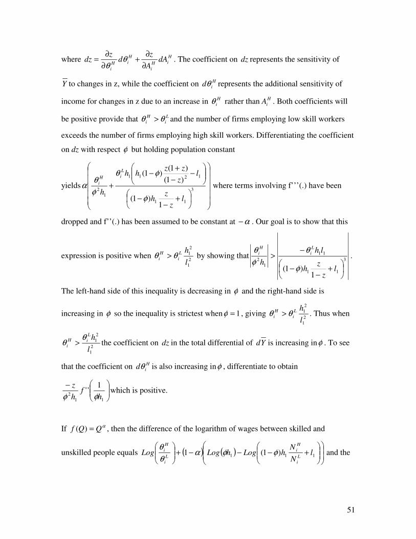
51

where HiH

i

HiH

i

dAAz

dz

dz∂∂+

∂∂= θθ

. The coefficient on dz represents the sensitivity of

Y to changes in z, while the coefficient on Hidθ represents the additional sensitivity of

income for changes in z due to an increase in Hiθ rather than H

iA . Both coefficients will

be positive provide that Li

Hi θθ > and the number of firms employing low skill workers

exceeds the number of firms employing high skill workers. Differentiating the coefficient

on dz with respect φ but holding population constant

yields

�����

�

�

�����

�

�

��

���

� +−

−

���

����

�−

−+−

+ 3

11

1211

12

1)1(

)1()1(

)1(

lz

zh

lz

zzhh

h

LiH

i

φ

φθ

φθα where terms involving f’’’(.) have been

dropped and f’’(.) has been assumed to be constant at α− . Our goal is to show that this

expression is positive when 21

21

lhL

iH

i θθ > by showing that 3

11

11

12

1)1( �

�

���

� +−

−

−>

lz

zh

lhh

Li

Hi

φ

θφθ

.

The left-hand side of this inequality is decreasing in φ and the right-hand side is

increasing in φ so the inequality is strictest when 1=φ , giving 21

21

lhL

iH

i θθ > . Thus when

21

21

lhL

iHi

θθ > the coefficient on dz in the total differential of Yd is increasing inφ . To see

that the coefficient on Hidθ is also increasing inφ , differentiate to obtain

���

����

�−

112

1''

hf

hz

φφwhich is positive.

If αQQf =)( , then the difference of the logarithm of wages between skilled and

unskilled people equals ( ) ( ) ��

�

�

��

�

����

����

�+−−−+��

�

����

�111 )1(1 l

NN

hLoghLogLogLi

Hi

Li

Hi φφα

θθ

and the

52

derivative of this with respect to φ equals

11

1

)1(

1

lNN

h

NN

h

Li

Hi

Li

Hi

+−+

φφ and this is increasing

with Li

Hi

NN

.