Direct Calculation of Cavity Noise

and Validation of Acoustic Analogies

Xavier Gloerfelt, Christophe Bailly and Daniel Juv�e

Laboratoire de M�ecanique des Fluides et d'Acoustique

Ecole Centrale de Lyon & UMR CNRS 5509

BP 163, 69131 Ecully cedex, France.

1. Introduction

Flow-induced cavity noise is a harmful noise source in many applications.1 A complex nonlin-

ear phenomenon is responsible for the intense self-sustained oscillations observed in experiments.

However, the pysics is di�cult to model analytically. The tonal Strouhal numbers are well approx-

imated by Rossiter's formula2 for a wide range of con�gurations but this simple semi-empirical

analysis is not able to indicate the main oscillation mode neither its amplitude. Moreover, it is now

generally recognized that noise generation mechanism can be dependent on the incoming boundary

layer, the geometric properties of the cavity, the Mach number of the mean ow, and many other

parameters. To predict detailed assessments of noise generation in complex cases, direct evaluation

from uid mechanics equations through DNS or LES with CAA tools represents the most thorough

technique currently available. Nevertheless, the storage requirement and computation time make

simulations of both the ow and acoustic �elds di�cult for realistic applications.

An alternative approach for computing the cavity noise consists of a two step calculation:

nonlinear generation of sound and linear sound propagation. Once sources have been identi�ed,

with CFD or CAA calculations, there are several techniques to calculate the resulting radiated

�eld. In this work, we propose to study numerical issues of three integral formulations: the Ffowcs

Williams and Hawkings (FW-H) analogy which extends Lighthill's theory to account for solid

boundaries and two Wave Extrapolation Methods (WEM) from a control surface, the Kirchho�

and porous FW-H methods. All these integral formulations have similar analytical insights based

on Green's function formalism and su�er from the limitation of the observer in a uniform ow. The

linear wave equation is assumed valid outside the source region, so that nonlinear propagation of

acoustic waves is also not described.

In the �rst part of this paper, we shall present the direct computation of Navier-Stokes equa-

tions for a two-dimensional rectangular cavity with aspect ratio of 2, matching one con�guration

of Karamcheti's experiments.3 In the second part, the far-�eld noise, associated with sources com-

puted from the previous DNS, is obtained using the three integral formulations. Each method shall

1

be described and the results shall be compared with those of direct acoustic simulation taken as a

reference.

2. Direct computation of cavity noise

2.1 Introduction

Despite the amount of numerical studies published on cavity ows, few deal with radiated noise.

Initial attemps have been made in supersonic cases, where acoustic �eld is dominated by shock

waves radiation. These CFD computations of compressible cavity ows used the two dimensional

unsteady RANS (Reynolds Averaged Navier-Stokes) equations with a turbulence model.4,5 The

�rst computations of acoustic radiation from a cavity with a subsonic grazing ow have been carried

out recently by Colonius et al.,6 and Shieh & Morris7 using 2-D Direct Numerical Simulation (DNS)

at a Reynolds number based on cavity depth ReD ' 5000. To investigate higher Reynolds numbers

(ReD ' 2 � 105), Shieh & Morris8 applied CAA tools to solve unsteady RANS with a turbulence

model: the one equation Spalart-Allmaras turbulence model and Detached Eddy Simulation have

been implemented.

In the present work, the tested con�guration is a 2-D rectangular cavity with L=D = 2, where

L = 5:18 mm is the cavity length and D = 2:54 mm is its depth. The incoming ow is a laminar

boundary layer with a Mach number M= 0:7 and a thickness � t 0:2D. The Reynolds number

chosen is ReD = 41000 in order to match Karamcheti's experiment.3 The latter studied the

acoustic radiation from two-dimensional rectangular cavities cut into a at surface at low Reynolds

numbers. The acoustic �elds were investigated by means of Schlieren observations, interferometry,

and hot-wire anemometer. In our simulation, the freestream air temperature T1 is 298.15 K and

the static pressure p1 is taken as 1 atm. The relatively thick incoming boundary layer ensures the

shear layer mode of oscillations.9 The choice of a high subsonic speed is interesting because the

frequency increases slightly with Mach number and the cavity is no more compact relatively to the

acoustic wavelength. Moreover, the test case is more relevant for integral methods because mean

ow e�ects on sound propagation are important.

2.2 Numerical procedure

A Direct Numerical Simulation (no turbulence model) of the 2-D compressible Navier-Stokes

equations is performed. These governing equations are discretized with a fourth order, seven-point

stencil, DRP di�erencing operator spatially, and are advanced in time with the use of an explicit

4th order Runge-Kutta scheme.9,10 Nonre ecting conditions are implemented to avoid spurious

re ections which can superpose to physical waves. To this end, the radiation boundary conditions

of Tam and Dong,11 using a polar asymptotic solution of the linearized Euler equations in the

acoustic far-�eld, are applied to the in ow and upper boundaries. At the out ow, we combine the

out ow boundary conditions of Tam and Dong, where the asymptotic solution is modi�ed to allow

2

the exit of vortical and entropic disturbances, with a sponge zone to dissipate vortical structures

in the region where the shear layer leaves the computational domain. This sponge zone uses grid

stretching and progressive additional damping terms.10 Along the solid walls, the nonslip condition

applies. The wall temperature Tw is calculated using the adiabatic condition. We keep centered

di�erencing at the wall to ensure su�cient robustness using ghost points.

The computational mesh is built up from nonuniform Cartesian grid with 147 � 161 points

inside the cavity and 501 � 440 outside, highly clustered near the walls. The minimum step size

corresponds to �y+min = 0:8 in order to resolve the viscous sublayer. The computational domain

extends over 8:5D vertically and 12D horizontally to include a portion of the radiated �eld. The

upstream and downstream boundaries are su�ciently far away from the cavity to avoid possible

self-forcing. The initial condition is a polynomial expression of the laminar Blasius boundary layer

pro�le with no forcing terms. Owing to the strong anisotropic computational mesh, we have a very

sti� discretized system. For explicit time marching schemes, an extremely small time step has to

be used in order to satisfy the stability CFL criterion: �t = 0:7 ��ymin=c1 = 6:06 � 10�9 s. A

selective damping, with a mesh Reynolds number of RS = 4:5, has to be introduced in order to

�lter out non physical short waves resulting from the use of �nite di�erences and/or treatment of

boundary conditions. It is applied a second time near the walls. The computation is 4 hours long

on a Nec SX-5.

2.3 Results and discussion

0 10 20 30 40 50 60 70 80−5000

−2500

0

2500

5000

t*U/D

p’ (

Pa)

a)

0 1 2 3 4 5 660

80

100

120

140

160

St

SP

L (d

B)

per

St

b)

Figure 1: a) Pressure history versus time, and b) Spectrum of pressure uctuations versus the Strouhalnumber St= fL=U1, at x=D = �0:04 and y=D = 2D.

Figure 1a gives a monitored pressure history in the near-�eld acoustic region. The ow reaches

a self-sustained oscillatory state after a time of about 25D=U1 but is still irregular until 65D=U1.

This transient time corresponds with the time needed by the recirculating ow to get installed in

the cavity. The associated sound pressure level spectrum is depicted in �gure 1b, and displays one

principal peak at St= 0:68. Several secondary peaks are noticeable and represent harmonics or

subharmonics of the fundamental mode f0. The experimental Strouhal number of oscillations is

St= 0:71. This error of 5% on the predicted frequency can be explained by the di�erent incoming

3

ow parameters or by the neglected 3-D e�ects.

A snapshot of vorticity depicted in �gure 2a shows the presence of two vortical structures

convected in the shear layer and impinging periodically the downstream edge of the cavity at

the frequency f0. The induced compression waves travel upstream and excite the shear layer at

the separation point near the leading edge, sustaining the oscillation process. The Rossiter semi-

empirical formula2 provides St= 0:71 for this con�guration with always two vortices in the shear

layer.

A Schlieren visualization, corresponding with vertical gradients of density, shows the struc-

ture of the radiated �eld in �gure 2b. Two wave patterns are visible for the positive gradients

(dark), which interfer during propagation. Their strong upstream directivity is characteristic of

high speed convection by the free stream. These radiations are in qualitatively good agreement

with the Schlieren picture taken from Karamcheti's experiment. From �nite-frange interferometry,

Karamcheti3 estimated an overall pressure level of about 160 dB at a distance of around three

cavity depths. The spectrum of �gure 1b indicates a level of 156 dB at 2:9D.

−1 0 1 2−1

0

x1/D

x 2/D

a)

b)

Figure 2: a) Snapshot of vorticity contours (16 contours between !D=U1 = �10:5 and 1:36: ( )negative contours, ( ) positive contours). b) Schlieren pictures corresponding to transversal derivativeof the density: present simulation on the left, Karamcheti's experiment3 on the right.

3. Validation of integral methods

Integral methods rest upon two principal physical backgrounds: �rst, the acoustic analogy which

split the computational domain in an aerodynamic region, where source terms responsible for noise

generation are built up, and an acoustic region governed by a linear wave equation; second, the

wave extrapolations which allow the evaluation of the far-�eld once some quantities are known on

a control surface.

Recent advances in integral methods were essentially developed for the reduction of helicopter

rotor noise12 and have been recently applied for the prediction of jet noise.13,14 Zhang, Rona, and

Lilley5 have used Curle's spatial formulation to obtain far-�eld spectra of cavity noise.

4

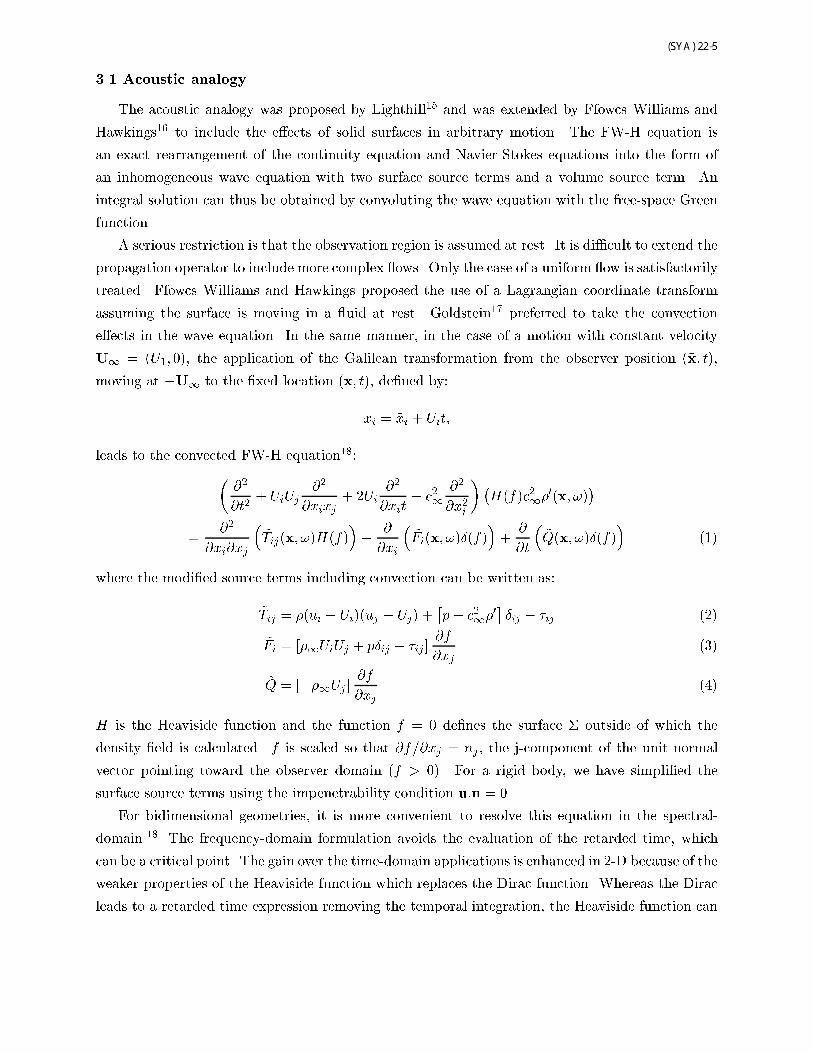
3.1 Acoustic analogy

The acoustic analogy was proposed by Lighthill15 and was extended by Ffowcs Williams and

Hawkings16 to include the e�ects of solid surfaces in arbitrary motion. The FW-H equation is

an exact rearrangement of the continuity equation and Navier-Stokes equations into the form of

an inhomogeneous wave equation with two surface source terms and a volume source term. An

integral solution can thus be obtained by convoluting the wave equation with the free-space Green

function.

A serious restriction is that the observation region is assumed at rest. It is di�cult to extend the

propagation operator to include more complex ows. Only the case of a uniform ow is satisfactorily

treated. Ffowcs Williams and Hawkings proposed the use of a Lagrangian coordinate transform

assuming the surface is moving in a uid at rest. Goldstein17 preferred to take the convection

e�ects in the wave equation. In the same manner, in the case of a motion with constant velocity

U1 = (U1; 0), the application of the Galilean transformation from the observer position (~x; t),

moving at �U1 to the �xed location (x; t), de�ned by:

xi = ~xi + Uit;

leads to the convected FW-H equation18:

�@2

@t2+ UiUj

@2

@xixj+ 2Ui

@2

@xit� c2

1

@2

@x2i

��H(f)c2

1�0(x; !)

�

=@2

@xi@xj

�~Tij(x; !)H(f)

��

@

@xi

�~Fi(x; !)�(f)

�+

@

@t

�~Q(x; !)�(f)

�(1)

where the modi�ed source terms including convection can be written as:

~Tij = �(ui � Ui)(uj � Uj) +�p� c2

1�0��ij � �ij (2)

~Fi = [�1UiUj + p�ij � �ij]@f

@xj(3)

~Q = [��1Uj ]@f

@xj(4)

H is the Heaviside function and the function f = 0 de�nes the surface � outside of which the

density �eld is calculated. f is scaled so that @f=@xj = nj , the j-component of the unit normal

vector pointing toward the observer domain (f > 0). For a rigid body, we have simpli�ed the

surface source terms using the impenetrability condition u:n = 0.

For bidimensional geometries, it is more convenient to resolve this equation in the spectral-

domain.18 The frequency-domain formulation avoids the evaluation of the retarded time, which

can be a critical point. The gain over the time-domain applications is enhanced in 2-D because of the

weaker properties of the Heaviside function which replaces the Dirac function. Whereas the Dirac

leads to a retarded time expression removing the temporal integration, the Heaviside function can

5

only change the upper limit of the integration to a �nite value, the lower limit remaining in�nite.

The spectral formulation removes this time constraint by solving FW-H equation harmonically.

With application of the Fourier transform:

F [�(x; t)] = �(x; !) =

Z1

�1

�(x; t)e�i!t dt (5)

equation (1) becomes�@2

@x2i+ k2 � 2iMik

@

@xi�MiMj

@2

@xi@xj

��H(f)c2

1�0(x; !)

�

= �@2

@xi@xj

�~Tij(x; !)H(f)

�+

@

@xi

�~Fi(x; !)�(f)

�� i! ~Q(x; !)�(f) (6)

where Mi = Ui=c1. A Green function for this inhomogeneous convected wave equation is obtained

from a Prandtl-Glauert transformation of the 2-D free-space Green's fonction in the frequency

domain:

G(x j y; !) =i

4�ei(Mk(x1�y1)=�2)H

(2)0

�k

�2r�

�(7)

where r� =p(x1 � y1)2 + �2(x2 � y2)2, H

(2)0 is the Hankel function of the second kind and order

zero, and � =p1�M2 is the Prandtl-Glauert factor, M< 1. The integral solution of equation (6)

is then given by:

H(f)p0(x; !) =�

Zf=0

~Fi(y; !)@G(x j y)

@yid��

Zf=0

i! ~Q(y; !)G(x j y) d�

�

ZZf>0

~Tij(y; !)@2G(x j y)

@yi@yjdy (8)

In 2-D, the volume integral is restricted to the surface including the aerodynamic sources Tij and

the surface integrals are calculated on the solid lines which represent rigid boundaries. We applied

the spatial derivatives on the Green function to avoid the evaluation of derivatives of aerodynamic

quantities. It is formally equivalent to the transformation in temporal derivatives as performed by

di Francescantonio19 or Farassat and Myers.20

3.2 Wave extrapolation methods

This kind of methods permits one to solve linear wave propagation problem once some ow

quantities are given on a closed �ctitious surface surrounding all the sources. The most famous one

is the Kirchho� method which makes a parallel with electromagnetism by using Kirchho�'s formula,

published in 1883. The use of the FW-H equation for a permeable surface can provide an alternative

extrapolation method as noted in the original Ffowcs Williams and Hawkings paper.16 This method

has been recently implemented by di Francescantonio.19 At nearly the same time, Brentner and

Farassat21 demonstrated the relationship between the FW-H equation and the Kirchho� equation

for moving surfaces. The FW-H and Kirchho� formulations solve the same physical problem, the

di�erences between the two writings being due to some choices made in the derivation process.

6

The main advantage of wave extrapolation methods with respect to acoustic analogy approaches

is that only surface integrals have to be evaluated because all non linear quadrupolar sources are

enclosed in the control surface. The problem is thus reduced by one dimension, which is particularly

interesting in a numerical point of view.

The convected Kirchho� method

For a moving medium, the acoustic pressure at an arbitrary point x and time t is related to

the distribution of sources within V and the distribution of the pressure and its derivative on the

boundary of V by the generalized Green's formula.17 For a 2-D con�guration, it can be written as:

H(f)p0(x; t) =

Z1

�1

ZZV (f>0)

(y; �)G(x; tjy; �) dyd�

+

Z1

�1

Z�(f=0)

�G@p

@yi� p

@G

@yi

�ni d�(y)d� +

U1

c21

Z1

�1

Z�(f=0)

�pDG

D��G

Dp

D�

�n1 d�(y)d�

where D=Dt is the time rate of change seen by an observer moving along with the mean ow.

Expressing the Green's function in the frequency-domain (7) and assuming all the quadrupolar

source are included in �, we obtain:

H(f)p0(x; !) =i�

4

Zf=0

�@p(y; !)

@n�H

(2)0

�k

�2r�

�+

k

�2p(y; !)

�@r�@n�

H(2)1

�k

�2r�

�

� iM@y1@n�

H(2)0

�k

�2r�

��� exp

�iMk(x1 � y1)

�2

��d�� (9)

where n� and d�� are the Prandtl-Glauert transforms of n and d�. This is the bidimensional

Kirchho� formulation for a uniformly moving medium in the frequency-domain.

The Ffowcs Williams and Hawkings WEM

This method is sometimes called the porous FW-H method because it coincides with the ap-

plication of the FW-H analogy on a �ctitious porous surface. The analytical developments are the

same that those of the FW-H analogy but the impenetrability condition is no more required, and,

on the contrary, one has to allow a uid ow across �. For a two-dimensional problem with uniform

subsonic motion, the FW-H WEM is given by equation (8) without the volume integral:

H(f)p0(x; !) = �

Zf=0

~Fi(y; !)@G(x j y)

@yid��

Zf=0

i! ~Q(y; !)G(x j y) d� (10)

with the two source terms:

~Fi = [�(ui � 2Ui)uj + �1UiUj + p�ij � �ij]@f

@xj(11)

~Q = [�uj � �1Uj]@f

@xj(12)

7

3.3 Numerical implementation

From an algorithmic point of view, there is almost no di�erence between the three integral

approaches considered here. The �rst step is the recording of the aerodynamic quantities during one

period of the DNS computation. The acoustic time step is 40 times the DNS time step corresponding

to 131 points per period. In the convected Kirchho� method, the pressure distribution and its

normal derivative over the three lines L1, L2, and L3 spanning the longitudinal direction are

needed to perform the surface integration. The normal derivative @p=@y2 is not directly available

from the near �eld solution and is here calculated with the DRP scheme. The variables (u1; u2; p; �)

are recorded on the same three �ctitious lines for the FW-H WEM, and on the walls of the cavity

and the surface around it for the FW-H analogy application as reported in �gure 3.

S

S1

22 D0 D

L

LL

123

-2 D

0.2 D0.5 D

1 D

-5 D 5 D

Figure 3: Schematic of the di�erent line and surface sources for evaluation of integral formulations.

The source terms are calculated and transformed in the frequency-domain using the Fourier

transform de�ned by (5). The integrals are then evaluated for each point of an acoustic meshgrid.

This regular cartesian grid of 176 � 184 points covers a area of (�5D; 5D) � (�1D; 8D), corre-

sponding with the main part of acoustic domain of DNS. Endly, an inverse Fourier transform is

used to recover the acoustic signal in time-domain.

3.4 Results and discussions

In the Kirchho� method, the results of the integration of (9) over L1, L2, and L3 are depicted

in �gure 4. Same results are obtained for the extrapolation using the permeable form of the FW-

H equation. The pressure �elds from integration over L1, L2, and L3 with source terms de�ned

by (11), and (12), and with M= 0:7 in the observer domain are compared in �gure 5. All the

computed far-�elds are consistent with that of DNS depicted in �gure 6b, even when the control

surface is located in the near-�eld region. The contour plots are only little sharper when the surface

is farther from sources because more nonlinear e�ects are included in the control surface. In this

con�guration, the additional nonlinear terms appearing in the surface integrals of FW-H WEM but

missing in the Kirchho� formulation as noted by Brentner and Farassat21 do not play a signi�cant

role and do not lead to the drastic di�erences observed in some previous comparisons when the

control surface is too close to the sources.21,22 Like di Francescantonio19 or Prieur and Rahier,23

we notice a similar behaviour of the two extrapolation methods. The advantage of porous FW-H

method is only the fact that it uses directly the quantities computed by direct simulation without

the need of further numerical process.

8

a) b) c)

Figure 4: Pressure �eld calculated at the same time by a) Kirchho�'s method from L1, b) Kirchho�'smethod from L2, c) Kirchho�'s method from L3.

a) b) c)

Figure 5: Pressure �eld calculated at the same time by a) FW-H WEM from L1, b) FW-H WEM from L2,c) FW-H WEM from L3.

When we apply FW-H analogy, the surface integrals are evaluated on the physical rigid walls

of the cavity and the volume integration is performed over the two surfaces S1 and S2 depicted in

�gure 3. The evaluation of volume integrals of Tij are sensible to truncature e�ets, especially in the

streamwise direction where the source terms decrease slowly. It is due to the presence of advected

vortices, ejected from the cavity during the clipping process, in the reattached boundary layer on

the downstream wall. By summing the volume and surface contributions (�g. 6a), we reconstruct

the total sound �eld in reasonably good agreement with the DNS reference solution of �gure 6b.

A quantitative comparison with the other methods is provided by the pressure pro�les and far-

�eld directivity of �gure 7. The results of the two WEM are similar and in fairly agreement with

the DNS reference solution whereas more di�erences can be seen for the acoustic analogy pro�le.

The main discrepancies for the directivity occur near the small angles � (i.e. in the downstream

direction) where the volume integration is abruptly cut by the end of the computational domain

at x1 = 5D, leading to truncature errors.

9

a) b)

Figure 6: Pressure �eld calculated at the same time by a) FW-H analogy (surface + volume integrals), b)DNS reference solution.

0 2 4 6 8 10−4000

−2000

0

2000

4000

p’ (

Pa)

r/D

a)

60 80 100 120 140 160 180132

142

152

162

θ (deg)

OA

SP

L(p’

) (

dB)

b)

Figure 7: a), Pressure pro�le along the line x1 + x2 = 2D (r =px21+ x2

2) b), Overall sound pressure level

as function of � measured from streamwise axis with center at the downstream edge of the cavity. () Kirchho�'s method from L1, ( ) FW-H WEM from L1, ( ) FW-H analogy, ( ) DNS.

However, FW-H analogy allows a better understanding of the structure of the radiated �eld than

WEM since the direct and re ected sound �eld can be separated. Following re ection's theorem

of Powell,24 we can indeed argue that the volume integral (�g. 8a) represents the direct radiated

�eld, and the surface integrals (�g. 8b) show essentially the re ected part of the �eld due to the

cavity walls. These two �elds at the same frequency give an interference �gure where the two waves

patterns are still distinguishable in our case because the cavity is not compact at the oscillation

frequency (L=� = 0:47).

The FW-H analogy provides more informations than the WEM but is more expensive in CPU

time because of the evaluation of volume integral (surface integral in 2-D) whereas wave extrapola-

tion methods need only surface integral (line integral in 2-D). For example, the computation time

needed by the FW-H WEM is around 13 minutes, whereas the FW-H analogy requires 17 hours, on

a Dec � computer. For the purpose of comparison, the DNS would take 320 hours on this machine.

10

a) b)

Figure 8: Pressure �eld obtained corresponding to: a) volume integral part of FW-H analogy, and b) surfaceintegral part of FW-H analogy.

4. Conclusion

In a �rst part, a direct calculation of the sound radiated by a ow over a 2-D rectangular cavity

is carried out. To this end, a DNS is performed using CAA numerical methods. This approach is

expensive but is able to give all the interactions between ow and acoustic, and provides a powerful

tool to determine noise generation mechanisms. The directly computed sound �eld is qualitatively

and quantitatively consistent with Karamcheti's measurements in the same con�guration.

The results of DNS are then successfully compared to three hybrid methods which use the

DNS aerodynamic quantities to solve integral formulations. The wave extrapolation methods, like

Kirchho�'s or porous FW-H methods, are relatively una�ected by the location of the control surface

and constitute interesting complementary tools to extend CAA near-�eld to the far-�eld. Acoustic

analogy is less e�cient because volume integrations are costly and sensible to truncature e�ects.

Nevertheless, it allows a separation between direct and re ected sound �elds, which is useful for an

analysis of radiation patterns.

To extend the present investigation, a 3-D simulation should be carried out. The recirculation

zone inside the cavity is indeed characterized by a three-dimensional turbulent mixing, even if the

development of the shear layer is almost two-dimensional. Such a study is under way.

Acknowledgments

Computing time is supplied by Institut du D�eveloppement et des Ressources en Informatique

Scienti�que (IDRIS - CNRS). The authors would like to thank Christophe Bogey for providing

ALESIA code, and for many useful discussions and suggestions during the course of this work.

References

1Rockwell, D., 1983, Oscillations of impinging shear layers, AIAA Journal, 21(5), p. 645{664.

11

2Rossiter, J.E. Wind-tunnel experiments on the ow over rectangular cavities at subsonic and transonicspeeds. Technical Report 3438, Aeronautical Research Council Reports and Memoranda, 1964.

3Karamcheti, K. Acoustic radiation from two-dimensional rectangular cutouts in aerodynamic surfaces.Tech. Note 3487, N.A.C.A., 1955.

4Hankey, W.L. & Shang, J.S., 1980, Analyses of pressure oscillations in an open cavity, AIAA Journal,18(8), p. 892{898.

5Zhang, X., Rona, A. & Lilley, G.M., 1995, Far-�eld noise radiation from an unsteady supersonic cavity,AIAA Paper 95-040.

6Colonius, T., Basu, A.J. & Rowley, C.W., 1999, Numerical investigation of the ow past a cavity,AIAA Paper 99-1912.

7Shieh, C.M. & Morris, P.J., 1999, Parallel numerical simulation of subsonic cavity noise, AIAA Paper

99-1891.

8Shieh, C.M. & Morris, P.J., 2000, Parallel computational aeroacoustic simulation of turbulent subsoniccavity ow, AIAA Paper 2000-1914.

9Gloerfelt, X., Bailly, C. & Juv�e, D., 2001, Computation of the noise radiated by a subsonic cavityusing direct simulation and acoustic analogy, AIAA Paper 2001-2226.

10Bogey, C., Bailly, C. & Juv�e, D., 2000, Numerical simulation of sound generated by vortex pairing ina mixing layer, AIAA Journal, 38(12), p. 2210{2218.

11Tam, C.K.W. & Dong, Z., 1996, Radiation and out ow boundary conditions for direct computation ofacoustic and ow disturbances in a nonuniform mean ow, J. Comput. Acous., 4(2), p. 175{201.

12Brentner, K.S., 2000, Modeling aerodynamically generated sound: Recent advances in rotor noise pre-diction, AIAA Paper 2000-0345.

13Colonius, T. & Freund, J.B., 2000, Application of Lighthill equation to a Mach 1.92 turbulent jet,AIAA Journal, 38(2), p. 368{370.

14Bogey, C., Bailly, C. & Juv�e, D., 2001, Noise computation using Lighthill's equation with inclusion ofmean ow - acoustics interactions, AIAA Paper 2001-2255.

15Lighthill, M.J., 1952, On sound generated aerodynamically I. General theory, Proc. of the Royal Society

of London, A 211, p. 564{587.

16Ffowcs Williams, J.E. & Hawkings, D.L., 1969, Sound generated by turbulence and surfaces in arbi-trary motion, Philosophical Transactions of the Royal Society, A264(1151), p. 321{342.

17Goldstein, M.E., 1976, Aeroacoustics, McGraw-Hill, New York.

18Lockard, D.P., 2000, An e�cient, two-dimensional implementation of the Ffowcs Williams and Hawkingsequation, J. Sound Vib., 229(4), p. 897{911.

19Di Francescantonio, P., 1997, A new boundary integral formulation for the prediction of sound radia-tion, J. Sound Vib., 202(4), p. 491{509.

20Farassat, F. & Myers, M.K., 1988, Extension of Kirchho�'s formula to radiation from moving surfaces,J. Sound Vib., 123(3), p. 451{460.

21Brentner, K.S. & Farassat, F., 1998, An analytical comparison of the acoustic analogy and Kirchho�formulation for moving surfaces, AIAA Journal, 36(8), p. 1379{1386.

22Singer, B.A., Brentner, K.S., Lockard, D.P. & Lilley, G.M., 2000, Simulation of acoustic scatteringfrom a trailing edge, J. Sound Vib., 230(3), p. 541{560.

23Prieur, J. & Rahier, G., 1998, Comparison of Ffowcs Williams-Hawkings and Kirchho� rotor noisecalculations, AIAA Paper 98-2376.

24Powell, A., 1960, Aerodynamic noise and the plane boundary, J. Acoust. Soc. Am., 32(8), p. 982{990.

12