Introduction to Cavity QEDFabian Grusdt

March 9, 2011

AbstractThis text arose in the course of the “Hauptseminar Experimentelle Quantenoptik” in WS 2010 at the

TU Kaiserslautern, organized by Prof. Ott and Prof. Widera. I want to give a short introduction - alsofrom the theoretical point of view - to the fascinating field of cavity quantum electrodynamics (CQED).Modern experiments (QND measurements on photons and photon blockade) are discussed and basicresults derived.

Contents

I. Introduction 1

II. The Jaynes-Cummings Model 1

III. Strong- and Weak- coupling regime 2

IV. Basic experimental techniques 2First proofs of strong coupling . . . . . . . . . . 2Atom traps inside cavities . . . . . . . . . . . . 3

V. QND measurements on single photons 3

VI. Photon blockade 5Photon blockade experiment . . . . . . . . . . . 5

VII. Acknowledgements 7

I. Introduction

Cavity QED investigates the interaction of singleatoms with single electromagnetic field modes. Toachieve the experimental goal of realizing such a sys-tem, effort was made and nowadays it is achievableeven for optical transitions. This paves the way formany interesting physical applications. Two of themost interesting ones are for sure the use of cavityQED for the construction of a quantum network (withthe aim to use it for quantum computational tasks)and on the other hand its usefulness for elementaryverifications of quantum mechanics.

II. The Jaynes-Cummings Model

In this section we want to introduce the importantJaynes-Cummings Hamiltonian describing a two-levelatom (consisting of states |g〉, |e〉 separated by ~ωA)

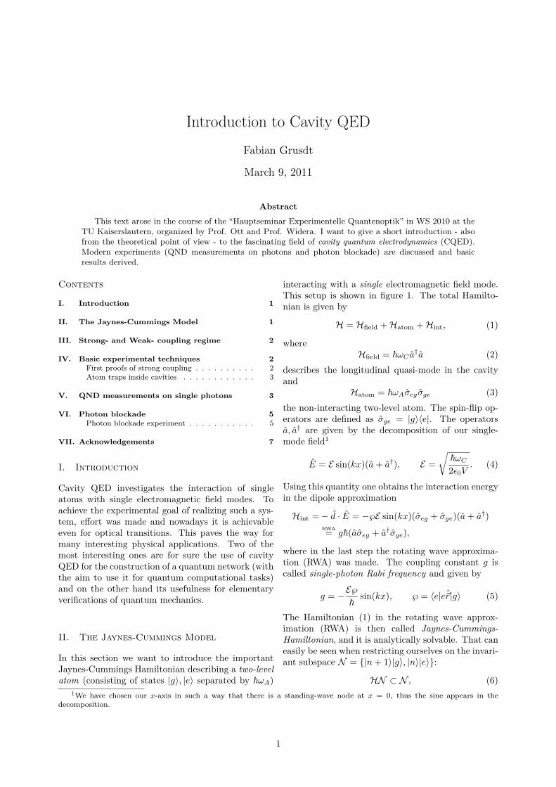
interacting with a single electromagnetic field mode.This setup is shown in figure 1. The total Hamilto-nian is given by

H = Hfield +Hatom +Hint, (1)

whereHfield = ~ωC a†a (2)

describes the longitudinal quasi-mode in the cavityand

Hatom = ~ωAσegσge (3)the non-interacting two-level atom. The spin-flip op-erators are defined as σge = |g〉〈e|. The operatorsa, a† are given by the decomposition of our single-mode field1

E = E sin(kx)(a+ a†), E =√

~ωC2ε0V

. (4)

Using this quantity one obtains the interaction energyin the dipole approximation

Hint =− d · E = −℘E sin(kx)(σeg + σge)(a+ a†)RWA= g~(aσeg + a†σge),

where in the last step the rotating wave approxima-tion (RWA) was made. The coupling constant g iscalled single-photon Rabi frequency and given by

g = −E℘~

sin(kx), ℘ = 〈e|e~r|g〉 (5)

The Hamiltonian (1) in the rotating wave approx-imation (RWA) is then called Jaynes-Cummings-Hamiltonian, and it is analytically solvable. That caneasily be seen when restricting ourselves on the invari-ant subspace N = |n+ 1〉|g〉, |n〉|e〉:

HN ⊂ N , (6)1We have chosen our x-axis in such a way that there is a standing-wave node at x = 0, thus the sine appears in the

decomposition.

1

|e〉

ωA

|g〉Γ

::::I

κ::::IωCxg x

→x↑y

Figure 1: The cavity QED parameters.

i.e. H is block-diagonal. Exact diagonalization of the2×2 blocks yields the eigenstates (dressed-states [15]):

|+, n〉 = sin θn|n〉|e〉+ cos θn|n+ 1〉|g〉,|−, n〉 = cos θn|n〉|e〉 − sin θn|n+ 1〉|g〉

with

cos θn =√

Ωn − δ2Ωn

, sin θn =√

Ωn + δ

2Ωn,

Ωn =√

4g2(n+ 1) + δ2, δ = ωA − ωC .

The eigenenergies of these dressed states are

E±,n = 12

~ωA + (n+ 1)~ωC ±12

~Ωn. (7)

They are compared to the case of vanishing couplingg = 0 in figure 2.

III. Strong- and Weak- coupling regime

The Jaynes-Cummings Hamiltonian does not includeany coupling to an environment leading to decay. Inorder to include the two loss-mechanisms, namelyspontaneous decay into the vacuum modes from |e〉(rate Γ) and decay of the field mode2 (rate κ), onehas to use a master equation(see e.g. [5]).It should - by physical understanding - be clear thatlarge losses, i.e. Γ, κ g lead to strong decay andthus no coherent evolution is expected. This case isreferred to as weak coupling regime. In the oppositecase Γ, κ g coherent evolution dominates for a verylong time, until dephasing destroys it. This case is re-ferred to as strong coupling regime. After some anal-ysis [5] it turns out that the cavity coupling leads to amodified decay rate of the atom. Both extreme casescan be found, that of enhanced and that of inhibitedspontaneous decay.

IV. Basic experimental techniques

In this section I want to discuss the basic experimen-tal techniques employed in cavity QED. One of the

main goals of modern experiments is to trap singleatoms long enough to perform quantum-logical oper-ations with them [3,4]. But there is also a second,reverse way of using cavity QED, where the field inhigh-Q cavities itself is measured via beams of Ry-dberg atoms[1]. These experiments (and also theirmethods) will be discussed in the following chapter.

First proofs of strong coupling

The first aim when dealing with cavity QED was toproof operation in the strong coupling regime. There-fore it was tried to measure the single-atom vacuumRabi splitting. A basic problem in the first experi-ments was that one couldn’t trap atoms in cavitiesbut only beams of atoms where available. The firstexperiment [7] that measured single atom transitsshall be presented in the following.The experimental setup is shown in figure 3 (a): Thecold atoms are provided by a Cesium-MOT some mil-limeters above the cavity. At the beginning of eachmeasurement the MOT is released and the atoms canescape. Some of them then pass through the cavityand interact with the field. The energy levels them-selves are recorded via the transmission of a probebeam incident on the cavity: The transmittance ishigh when the probe laser is on resonance with acavity mode. When an atom enters, it acts like adispersive medium and thus the mode energies areeffectively shifted. The shift is given by the vacuumRabi splitting g (provided there are no (e.g. thermal)photons inside the cavity, which is very unlikely foroptical frequencies).In order to make sure that only a single atom is insidethe cavity at a time, a second probe laser is used tomonitor the transit of single atoms. Therefore thesecond probe laser is held at zero detuning (relativeto ωC). When an atom enters, the transmittanceof this second laser decreases dramatically and thepresence of a single atom is shown.

2In the experiment this decay is usually caused by mirror imperfections.

2

ωC = ωA

ωC = ωA

|0〉|g〉

|1〉|g〉|0〉|e〉

|2〉|g〉|1〉|e〉

|0〉

|−, 0〉

|+, 0〉

|−, 1〉

|+, 1〉

√2g↓

g↓

Figure 2: The Jaynes-Cummings energy levels for zero detuning δ = 0. Left: g = 0, right: g 6= 0.

(a) (b)

Figure 3: Experimental setup (a) and single atom vacuum Rabi splitting (b) as main result of [7]. Themeasurement in explained in the text below.

Atom traps inside cavities

It is very desirable to trap a single atom for a longtime inside an optical cavity. There exist proposalshow one can then couple many such cavity-atom sys-tems to implement quantum networks [3], or how toperform quantum computation with the neutral atomground states as qubits [4].For trapping single atoms dipole traps are standard.In order to not disturb the cavity mode used forthe CQED setup one uses far off-resonance traps(FORTs). The needed additional laser beam can becoupled into a TEM00 cavity mode besides a standardprobe beam for example. The central experimentalproblem is the finite trapping time of the atom. Itis limited by several heating mechanisms (discussede.g. in [8,9,10]). Additionally the two levels needed|e〉 and |g〉 experience different AC-Stark shifts, de-phasing the coherent evolution of the system.However the mentioned problems could be solvedby using a specific trapping wavelength called magicwavelength. It depends on the sort of atoms used. In[10] a trapping mechanism based on the magic wave-length λCs = 935 nm for Cesium is reported wherethe authors reach an atomic trapping time of 2− 3s.

V. QND measurements on single photons

The group of Haroche at ENS in Paris succeeded inperforming non-destructive measurements on singlephotons trapped inside a high-Q cavity [1,2] wherethe photon is not lost in the process. These processesare expected to be described by the quantum mechan-ical postulates of measurements.They used the dispersive interaction of single atomswith the trapped intra-cavity-photons in the strongcoupling regime to perform a measurement on thefield via atoms. Therefore they need atomic stateswith a long enough lifetime for the detection, pro-vided by circular Rydberg atoms. These are atomsin states with a high principle quantum number n(n = 50 in the experiment) and the highest possibleangular and magnetic quantum numbers:

l = n− 1 |ml| = n− 1 (8)

These states have radiative lifetimes of about a factor1000 larger than their corresponding low-l states, andin the experiment they were of the order τ = 30ms.The atomic transition used (n = 50 ↔ n = 51) is inthe microwave regime and thus a microwave cavity isused. It is constructed of superconducting niobiummirrors (separated 27mm apart from each other) andreaches a photon storage time T ≈ 0.13 s. Together

3

Figure 4: The setup of the experiment described in the text, [1,2].

|e〉

|g〉l- - -

δ

ωC

π2 Φ π

2

CR1 R2 D

Figure 5: The working principle of the Ramsey interferometer used to measure the state of the intra-cavityfield.

with the cavity resonance used at ωC/2π = 51.1GHzthis yields a Q-value3 of Q ≈ 4 · 1010 4. In orderto avoid thermal radiation the whole setup us cooleddown to 0.8K. The maximal coupling strength isgiven by g0/2π = 51 kHz while the detuning betweencavity resonance and atomic transition is δ/2π =67 kHz. Thus |δ| ≥ |g0| which is required for the Ram-sey interferometer that shall be discussed now.In order to detect the coherent atom-light interaction,the high-Q cavity C is sandwiched by two additionalcavities (R1, R2) forming an atomic Ramsey interfer-ometer, see figure 4. Its working principle is shownfigure 5. Atoms optically pumped into |g〉 are pre-pared in a superposition state by applying a π/2-pulsein R1. They fly through the cavity where they inter-act with the field-mode. In their first QND experi-ment [1] the Paris group considered only field states5

of at maximum one photon:

|Ψfield〉 = c0|0〉+ c1|1〉. (9)The atom-cavity interaction can be understood as anadiabatic following of the Jaynes-Cummings statesand when properly adjusted the result is the follow-ing:

|n〉 = |0〉 ↔ Φ = π

|n〉 = |1〉 ↔ Φ = 2π

where Φ stands for the rotation angle of the atomicstate vector around the Bloch-sphere z-axis. This re-sult is obtained assuming adiabatic following of theatomic states when passing C. The adiabaticity con-dition then gives the restriction mentioned above,|δ| ≥ |g0|. After this process another classical π/2-pulse is applied in R2, leading to the final atomicstates |Ψatom〉:

|n〉 = |0〉 ↔ |Ψatom〉 = |g〉|n〉 = |1〉 ↔ |Ψatom〉 = |e〉.

The state-sensitive detectors D1 and D2 can thus (in-directly) measure the state of the intra-cavity field.To be precise, they only measure whether the photonnumber is odd or even since within the experimen-tal errors |0〉 and |2〉 photon states yield the sameprobability for detecting the atom in |e〉. In [2] theexperimental setup was then refined such that up ton = 7-photon-states can be subsequently measured inthe same way. In this case, of course, several atomsare needed to gain complete information about thefield-state.After having understood how the measurement workswe will now discuss some of the results. The main goalof the experiment was to confirm the quantum me-chanical postulates. In [1] two kinds of experiments

3The Q-value is used to characterize the quality of a cavity. It is defined as Q = ωCκ

.4This is the highest Q-value ever achieved with a cavity so far.5The atomic states are not to be mistaken for the field states. Here |n〉, for n an integer, denotes field states while |e〉, |g〉

denote the atomic ones.

4

(A) (B)

Figure 6: (A) Birth and death of thermal intra-cavity photons observed with the method explained in thetext. (B) Loss of one prepared intra-cavity photon (upper case) and average over 904 such measurements(lower case). All from [1].

were performed on the field subspace consisting of |0〉and |1〉. In the first, thermal photons were continu-ously observed, an example is shown in figure 6 (A).One can clearly distinguish between the one photonstate and vacuum although there are several unex-pected events caused by experimental imperfections.In the second experiment the field state |1〉 was pre-pared in a controlled way by sending through the cav-ity an atom in |e〉. Its interaction time inside the cav-ity was adjusted such that the atom exits the cavityin |g〉 and a photon is left in the cavity field. Af-terwards the decay of these photons is observed likebefore, see figure 6 (B). In the upper diagram a singlemeasurement is shown while in the lower the aver-age over 904 such single ones was calculated. Theexpected quantum-jump behavior for single events aswell as the smooth exponential decay of the ensemble-average can clearly be seen.

VI. Photon blockade

In this last section we will discuss how one can utilizecavity QED for strong photon-photon interactions.These can be used to create non-classical states oflight. I will present an experiment [12] based on atheoretical proposal [11] for creating such states.

Photon blockade experiment

The experiment reported here [12] was performed atthe CALTECH in 2005 by Birnbaum et. al. The basicidea was to use the Jaynes-Cummings anharmonicityof a single trapped atom in a high-Q optical cavityto reach strong enough photon-photon interaction. If

these interactions are large enough (i.e. if the addi-tional energy needed to place a second photon intothe cavity besides ~ωC is large enough) only one orno photon can populate the cavity mode due to en-ergy conservation. This phenomenon is referred to asphoton blockade. The required large non-linearity isachieved here by strong atom-field coupling, i.e. largeg. Photon blockade can be observed by examinationof the photon statistics6 of light transmitted troughthe cavity mirrors: sub-poissonian and anti-bunchedlight is expected.The experimental parameters are:

(gmax,Γ, κ) /2π = (34, 2.6, 4.1)MHz. (10)

Thus the setup is far in the strong coupling regime.The photon-photon interaction for a two-level systemcan be deduced from figure 2. We assume a pump-beam with photon energy ~ω0 = E−,0 − E0 and zerodetuning δ = 0 between cavity-mode and atomic tran-sition. Thus |0,−〉 can be populated. If an additionalphoton shall populate the cavity, the lowest possibleenergy state is |1,−〉. This yields an estimate for thephoton-photon interaction energy

~γ ≈ E−,1 − 2~ω0 = (2−√

2)g ≈ ~ · 20MHz · 2π,

which is large compared to the typical line widthwhich is of the order ~κ. From the latter it is clearthat photon-photon interactions give a substantialcontribution. The assumption of one cavity mode anda simple two-level system however is not justified fora realistic system. In the actual experiment two or-thogonally polarized cavity modes ly,z are present andatomic cesium was used. The atomic transition is theCs D2-line 6S1/2, F = 4 → 6P3/2, F

′ = 5′ and themanifold of hyperfine sub-levels has to be taken into

6For details about photon statistics the reader is referred to e.g. [5].

5

Figure 7: Energy levels of the full hyperfine-manifold dressed states of the Cs D2-line. ω0 ≡ ωC = ωA wasassumed. From [12].

(a) (b)

Figure 8: (a) Experimental setup. (b) Theoretical calculation (steady-state solution to the full master equa-tion) for a two-level system (left) and the actual Cs D2-transition manifold in the experiment. Both from[12].

(a) (b)

Figure 9: (Measurement result around τ = 0, (a), and on longer time scales (b) . Both from [12].

6

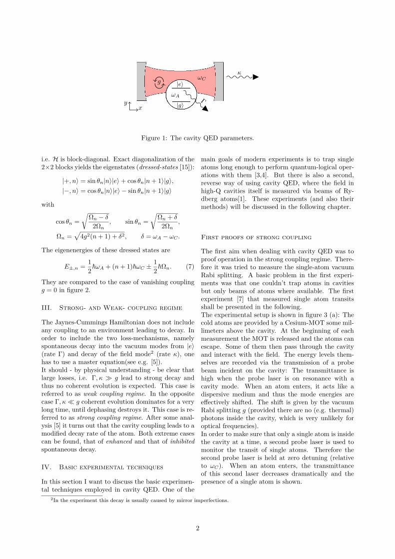
account. Exact diagonalization of the correspond-ing Hamiltonian yields the dressed-states energy lev-els given in figure 7. The photon-photon interactionis still of the order of γ calculated for the two-levelmodel above.Next, the experimental setup (see figure 8 (a)) shallbe discussed. A probe beam E(y,z)

p incident on mir-ror M1, polarized in y- or z-direction respectively,drives the cavity. Inside the latter a single Cs-atom istrapped in a FORT and there are further laser beamsfor cooling and testing (for details, see [12]). Behindthe second mirror M2 only the z-polarized light canpass the polarizing beam splitter PBS. Then g(2)(τ) ofthe transmitted field Ezt is measured via coincidencesof D1 and D2

7. For this setup the steady-state solu-tion of the full master-equation is shown in figure 8(b), once for the simple two-level model and for theactual Cs-atom. In the latter case Tzz (Tyz) refers tothe transmittance of light from lz (ly)8 into lz andanalogously g(2)

zz (g(2)yz ) refers to the second-order cor-

relation function of the transmitted lz-light for inci-dent lz (ly) light. One sees that the realistic systemqualitatively behaves like the two-level system. Thetransmittance has just got more structures aroundthe vacuum-Rabi peaks due to the additional states.The correlation functions can at least partly be un-derstood. Around ωp − ω0 = gmax ≡ g0 all plots ex-hibit sub-poissonian statistics. This can most clearlybe seen at g(2)

yz (τ). These statistics can be understoodas a direct consequence of photon-blockade: Only onephoton at a time can populate the cavity-mode. So wealso expect photon anti-bunching for this frequency.One also clearly sees peaks at about ωp = ω0±g0/

√2,

at two-photon resonance. Here the field shows super-poissonian statistics g(2)(0) 1. For more details,

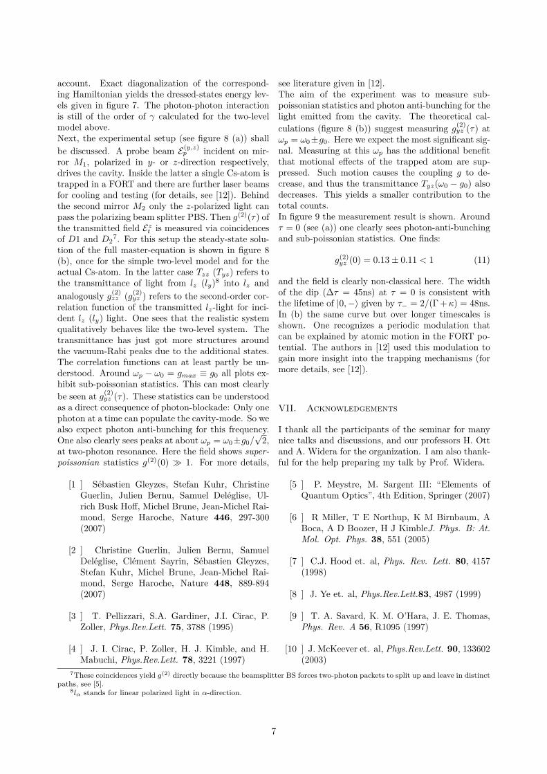
see literature given in [12].The aim of the experiment was to measure sub-poissonian statistics and photon anti-bunching for thelight emitted from the cavity. The theoretical cal-culations (figure 8 (b)) suggest measuring g(2)

yz (τ) atωp = ω0±g0. Here we expect the most significant sig-nal. Measuring at this ωp has the additional benefitthat motional effects of the trapped atom are sup-pressed. Such motion causes the coupling g to de-crease, and thus the transmittance Tyz(ω0 − g0) alsodecreases. This yields a smaller contribution to thetotal counts.In figure 9 the measurement result is shown. Aroundτ = 0 (see (a)) one clearly sees photon-anti-bunchingand sub-poissonian statistics. One finds:

g(2)yz (0) = 0.13± 0.11 < 1 (11)

and the field is clearly non-classical here. The widthof the dip (∆τ = 45ns) at τ = 0 is consistent withthe lifetime of |0,−〉 given by τ− = 2/(Γ +κ) = 48ns.In (b) the same curve but over longer timescales isshown. One recognizes a periodic modulation thatcan be explained by atomic motion in the FORT po-tential. The authors in [12] used this modulation togain more insight into the trapping mechanisms (formore details, see [12]).

VII. Acknowledgements

I thank all the participants of the seminar for manynice talks and discussions, and our professors H. Ottand A. Widera for the organization. I am also thank-ful for the help preparing my talk by Prof. Widera.

[1 ] Sébastien Gleyzes, Stefan Kuhr, ChristineGuerlin, Julien Bernu, Samuel Deléglise, Ul-rich Busk Hoff, Michel Brune, Jean-Michel Rai-mond, Serge Haroche, Nature 446, 297-300(2007)

[2 ] Christine Guerlin, Julien Bernu, SamuelDeléglise, Clément Sayrin, Sébastien Gleyzes,Stefan Kuhr, Michel Brune, Jean-Michel Rai-mond, Serge Haroche, Nature 448, 889-894(2007)

[3 ] T. Pellizzari, S.A. Gardiner, J.I. Cirac, P.Zoller, Phys.Rev.Lett. 75, 3788 (1995)

[4 ] J. I. Cirac, P. Zoller, H. J. Kimble, and H.Mabuchi, Phys.Rev.Lett. 78, 3221 (1997)

[5 ] P. Meystre, M. Sargent III: “Elements ofQuantum Optics”, 4th Edition, Springer (2007)

[6 ] R Miller, T E Northup, K M Birnbaum, ABoca, A D Boozer, H J KimbleJ. Phys. B: At.Mol. Opt. Phys. 38, 551 (2005)

[7 ] C.J. Hood et. al, Phys. Rev. Lett. 80, 4157(1998)

[8 ] J. Ye et. al, Phys.Rev.Lett.83, 4987 (1999)

[9 ] T. A. Savard, K. M. O’Hara, J. E. Thomas,Phys. Rev. A 56, R1095 (1997)

[10 ] J. McKeever et. al, Phys.Rev.Lett. 90, 133602(2003)

7These coincidences yield g(2) directly because the beamsplitter BS forces two-photon packets to split up and leave in distinctpaths, see [5].

8lα stands for linear polarized light in α-direction.

7

[11 ] A. Imamoglu, H. Schmidt, G. Woods, and M.Deutsch, Phys.Rev.Lett. 79, 1467 (1997)

[12 ] K.M. Birnbaum, A. Boca, R. Miller, A.D.Boozer, T.E. Northup, H.J. Kimble, Nature436, 87-90 (2005)

[13 ] M. Fleischhauer, A. Imamoglu, J.P. Maran-

gos, Rev.Mod.Phys 77, 633 (2005)

[14 ] Boca A, Miller R, Birnbaum K M, BoozerA D, McKeever J and Kimble H J, Phys. Rev.Lett. 93, 233603 (2004)

[15 ] C.N. Cohen-Tannoudji, Nobel Lecture, De-cember 8, 1997

8