dimension reduction techniques - stanford...

Dimension Reduction Techniques, (MMDS) June 24, 2006 1

Dimension Reduction Techniques

for Efficiently Computing Distances in Massive Data

Workshop on Algorithms for Modern Massive Data Sets

June 22, 2006

Ping Li, Trevor Hastie, and Kenneth Church (MSR)

Department of Statistics

Stanford University


Let’s Begin with AAT

The data matrix A ∈ Rn×D consists of n rows (data points) in R

D , D

dimensions (features or attributes).

* * * * *...

* * * * *...

* * * * *...

* * * * *...

* * * * *...

t

u 1

1 t t t2 3 4

u

u

u

t D

2

3

4

u n

...

... ... ...... ... ... ...

A =

What is the cost of computing AAT ? O(n2D) A big deal ?

What if n = 0.6 million, D = 70 million? n2D = 2.5× 1019. Take a while!

Why do we care about AAT ? Useful for a lot of things.


• [AAT]1,2 = uT

1u2 =∑D

j=1 u1,ju2,j

is the inner product, an important measure of vector similarity.

• [AAT] is fundamental in distance-based clustering, support vector machine

(SVM) kernels, information retrieval, and more.

• An example. Ravichandran et. al. (ACL 2005) found the top similar nouns for

each of n = 655, 495 nouns, from a collection of D=70 million Web pages.

Brute-force O(n2D) ≈ 1019 may take forever. They used random

projections.

Other similarity or dissimilarity measures

• l2 distance: ‖u1 − u2‖22 =

∑Dj=1(u1,j − u2,j)

2.

• l1 distance: ‖u1 − u2‖1 =∑D

j=1 |u1,j − u2,j |

• Multi-way inner product:∑D

j=1 u1,ju2,ju3,j


Let’s Approximate AAT and Other Distances

Many reasons why approximation is a good idea.

• Exact computation could be practically infeasible.

• Often do not need exact answers. Distances are used by other tasks such as

clustering, retrieval, and ranking, which introduce errors.

• An approximate solution may help finding the exact solution more efficiently.

Example: Databases query optimization


What Are Real Data Like?: Google Page Hits

Query Hits (Google)

A 22,340,000,000

Function words The 20,980,000,000

Frequent words Country 2,290,000,000

Knuth 5,530,000

Names ”John Nash” 1,090,000

Kalevala 1,330,000

Rare words Griseofulvin 423,000

• Term-by-document matrix (n by D) is huge, and highly sparse

• Approx n = 107 (interesting) words/items

• Approx D = 1010 Web pages (indexed)

• Lots of large counts (even for so-called rare words)


Outline of the Talk

• Two strategies (besides SVD) for dimension reduction:

• Sampling

• Sketching

• Normal random projections (for l2).

• Cauchy random projections (for l1). A case study on Microarray Data.

• Conditional Random Sampling (CRS), a new sketching algorithm for sparse

data: Sampling + sketching

• Comparisons.


Strategies for Dimension Reduction: Sampling and Sketching

Sampling: Randomly pick k (out of D) columns from the data matrix A.

1

2

345

n

...

1 2 3 4 5 6 7 ... ... Duuuuu

u

A ∈ Rn×D =⇒ A ∈ R

n×k

(uT1u2 =

∑Dj=1 u1,ju2,j) ≈ (uT

1u2 =∑k

j=1 u1,j u2,j) ×Dk

• Pros: Simple, popular, generalizes beyond approximating distances

• Cons: No accuracy guarantee. Large errors for worst case (heavy-tailed

distributions). Mostly “zeros” in sparse data.


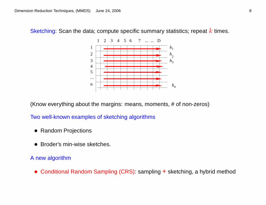
Sketching: Scan the data; compute specific summary statistics; repeat k times.

1

2

345

n

...

1 2 3 4 5 6 7 ... ... D

1

2

n

3

h

h

h

h

(Know everything about the margins: means, moments, # of non-zeros)

Two well-known examples of sketching algorithms

• Random Projections

• Broder’s min-wise sketches.

A new algorithm

• Conditional Random Sampling (CRS): sampling + sketching, a hybrid method


Random Projections: A Brief Introduction

Let B = AR, A ∈ Rn×D is the original data matrix. R ∈ R

D×k is the

random projection matrix. B ∈ Rn×k is the projected data.

A R = B

Estimate original distances from B. (Vempala 2004, Indyk FOCS00,01)

• For l2 distance, use R with entries of i.i.d. Normal N(0, 1).

• For l1 distance, use R with entries of i.i.d. Cauchy C(0, 1).

Computational cost: O(nDk) for generating the sketch B.

O(n2k) for computing all pairwise distances. k � min(n, D).

O(nDk + n2k) is a huge reduction, from O(n2D).


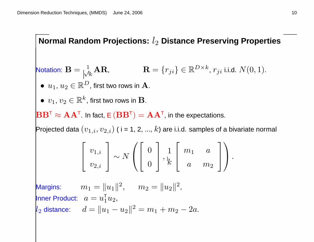
Normal Random Projections: l2 Distance Preserving Properties

Notation: B = 1√kAR, R = {rji} ∈ R

D×k, rji i.i.d. N(0, 1).

• u1, u2 ∈ RD , first two rows in A.

• v1, v2 ∈ Rk , first two rows in B.

BBT ≈ AA

T. In fact, E (BBT) = AA

T, in the expectations.

Projected data (v1,i, v2,i) ( i = 1, 2, ..., k) are i.i.d. samples of a bivariate normal

v1,i

v2,i

∼ N

0

0

,1

k

m1 a

a m2

.

Margins: m1 = ‖u1‖2, m2 = ‖u2‖

2,

Inner Product: a = uT1u2,

l2 distance: d = ‖u1 − u2‖2 = m1 + m2 − 2a.


v1,i

v2,i

∼ N

0

0

,1

k

m1 a

a m2

.

Linear estimators (sample distances are unbiased for original distances)

a = vT1v2 =

k∑

i=1

v1,iv2,i, E(a) = a

d = ‖v1 − v2‖2 =

k∑

i=1

(v1,i − v2,i)2, E(d) = d

However

Marginal norms m1 = ‖u1‖2, m2 = ‖u2‖

2 can be computed exactly

BBT ≈ AA

T, but at least we can make the diagonals exact (easily).

And off-diagonals can be improved (a little bit more work)


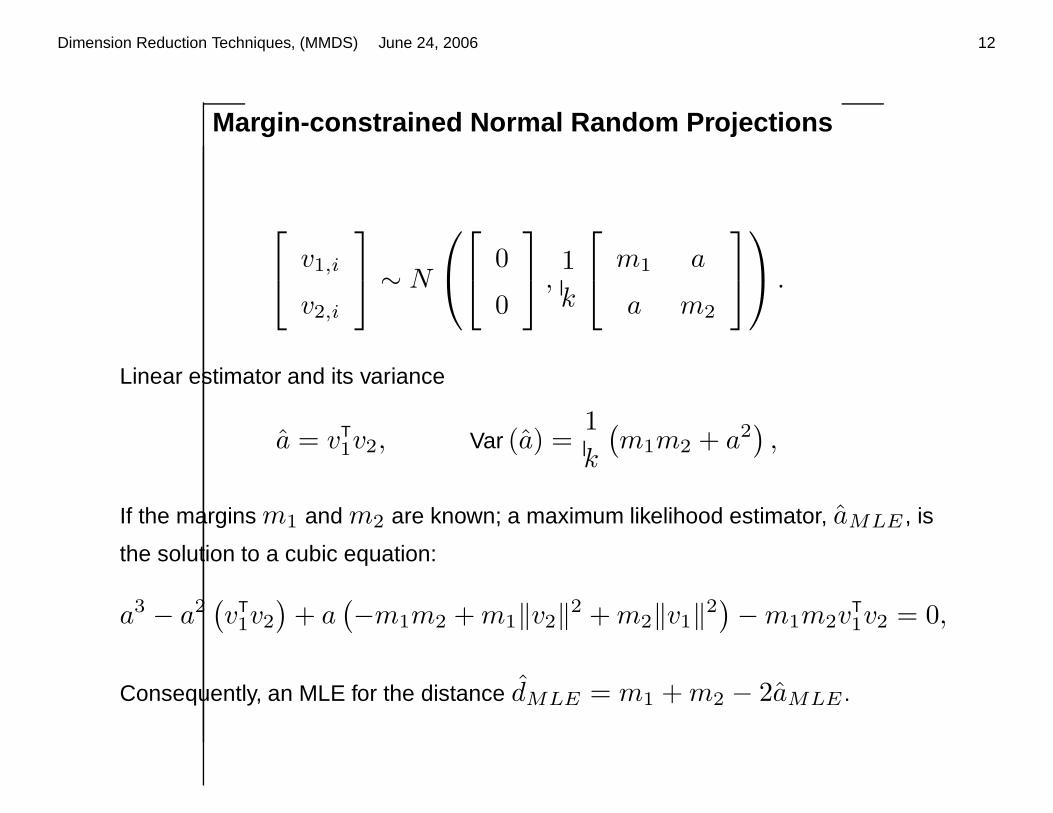
Margin-constrained Normal Random Projections

v1,i

v2,i

∼ N

0

0

,1

k

m1 a

a m2

.

Linear estimator and its variance

a = vT1v2, Var (a) =

1

k

(

m1m2 + a2)

,

If the margins m1 and m2 are known; a maximum likelihood estimator, aMLE , is

the solution to a cubic equation:

a3 − a2(

vT1v2

)

+ a(

−m1m2 + m1‖v2‖2 + m2‖v1‖

2)

− m1m2vT1v2 = 0,

Consequently, an MLE for the distance dMLE = m1 + m2 − 2aMLE .


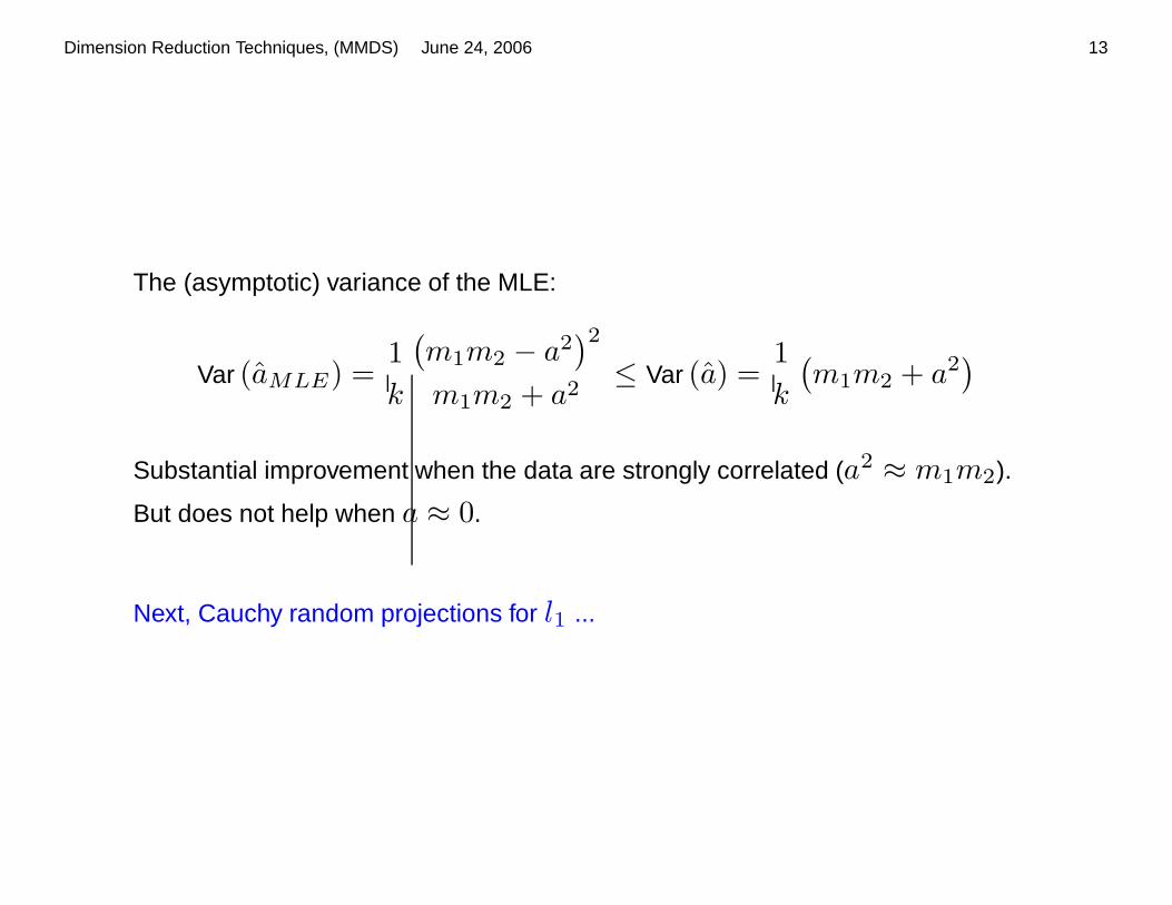
The (asymptotic) variance of the MLE:

Var (aMLE) =1

k

(

m1m2 − a2)2

m1m2 + a2≤ Var (a) =

1

k

(

m1m2 + a2)

Substantial improvement when the data are strongly correlated (a2 ≈ m1m2).

But does not help when a ≈ 0.

Next, Cauchy random projections for l1 ...


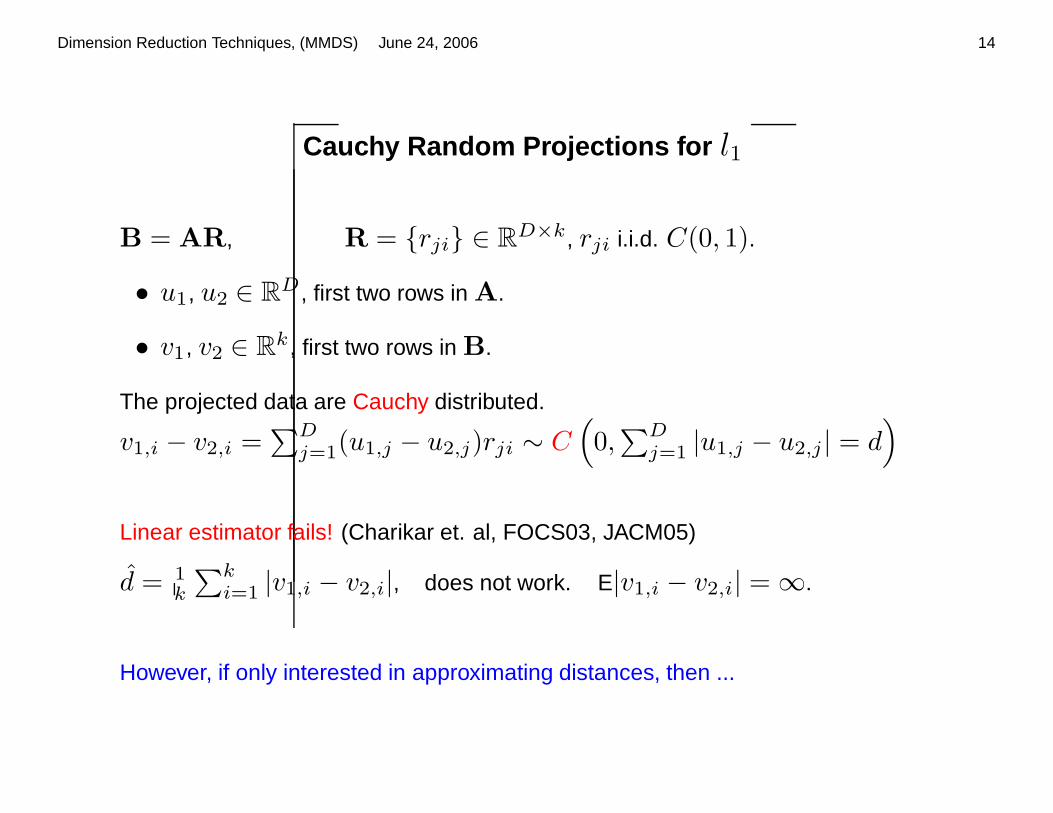
Cauchy Random Projections for l1

B = AR, R = {rji} ∈ RD×k, rji i.i.d. C(0, 1).

• u1, u2 ∈ RD , first two rows in A.

• v1, v2 ∈ Rk , first two rows in B.

The projected data are Cauchy distributed.

v1,i − v2,i =∑D

j=1(u1,j − u2,j)rji ∼ C(

0,∑D

j=1 |u1,j − u2,j | = d)

Linear estimator fails! (Charikar et. al, FOCS03, JACM05)

d = 1k

∑ki=1 |v1,i − v2,i|, does not work. E|v1,i − v2,i| = ∞.

However, if only interested in approximating distances, then ...


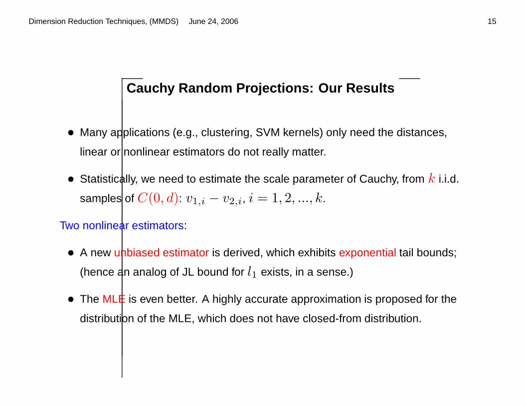
Cauchy Random Projections: Our Results

• Many applications (e.g., clustering, SVM kernels) only need the distances,

linear or nonlinear estimators do not really matter.

• Statistically, we need to estimate the scale parameter of Cauchy, from k i.i.d.

samples of C(0, d): v1,i − v2,i, i = 1, 2, ..., k.

Two nonlinear estimators:

• A new unbiased estimator is derived, which exhibits exponential tail bounds;

(hence an analog of JL bound for l1 exists, in a sense.)

• The MLE is even better. A highly accurate approximation is proposed for the

distribution of the MLE, which does not have closed-from distribution.


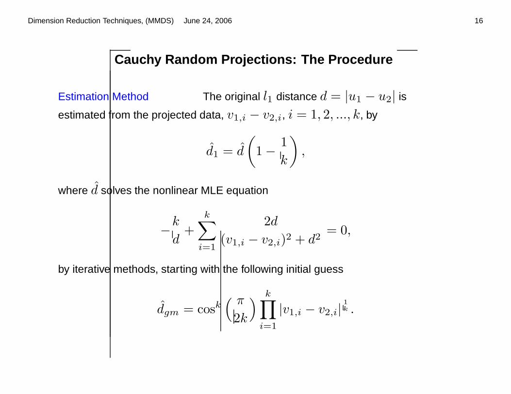
Cauchy Random Projections: The Procedure

Estimation Method The original l1 distance d = |u1 − u2| is

estimated from the projected data, v1,i − v2,i, i = 1, 2, ..., k, by

d1 = d

(

1 −1

k

)

,

where d solves the nonlinear MLE equation

−k

d+

k∑

i=1

2d

(v1,i − v2,i)2 + d2= 0,

by iterative methods, starting with the following initial guess

dgm = cosk( π

2k

)

k∏

i=1

|v1,i − v2,i|1

k .


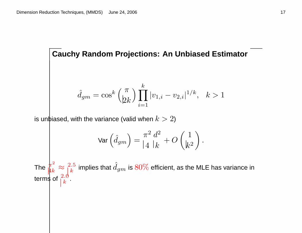
Cauchy Random Projections: An Unbiased Estimator

dgm = cosk( π

2k

)

k∏

i=1

|v1,i − v2,i|1/k, k > 1

is unbiased, with the variance (valid when k > 2)

Var(

dgm

)

=π2

4

d2

k+ O

(

1

k2

)

.

The π2

4k ≈ 2.5k implies that dgm is 80% efficient, as the MLE has variance in

terms of 2.0k .


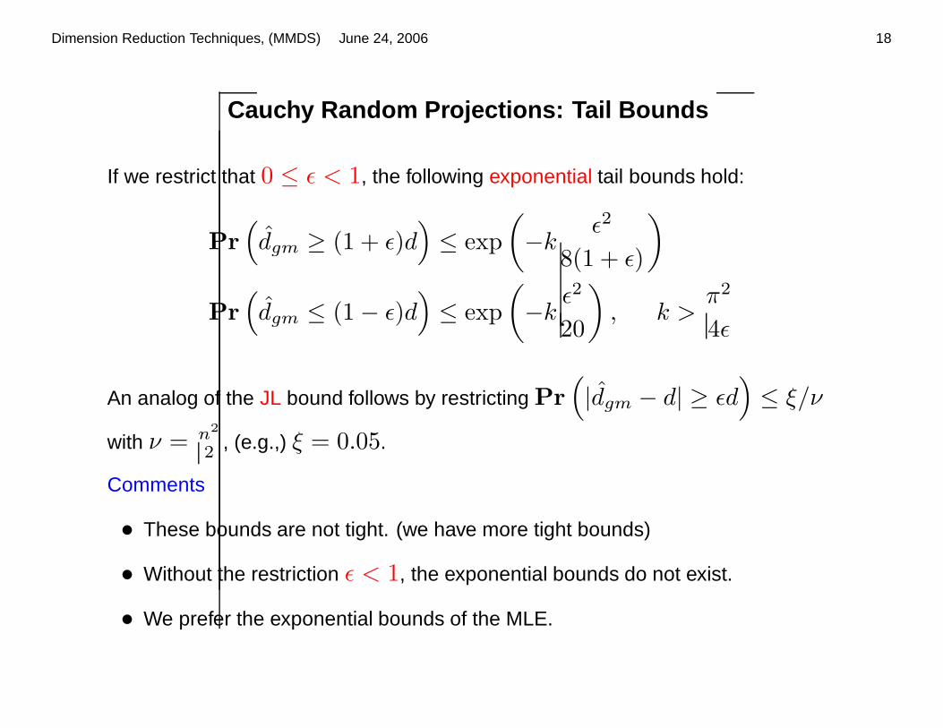
Cauchy Random Projections: Tail Bounds

If we restrict that 0 ≤ ε < 1, the following exponential tail bounds hold:

Pr

(

dgm ≥ (1 + ε)d)

≤ exp

(

−kε2

8(1 + ε)

)

Pr

(

dgm ≤ (1 − ε)d)

≤ exp

(

−kε2

20

)

, k >π2

4ε

An analog of the JL bound follows by restricting Pr

(

|dgm − d| ≥ εd)

≤ ξ/ν

with ν = n2

2 , (e.g.,) ξ = 0.05.

Comments

• These bounds are not tight. (we have more tight bounds)

• Without the restriction ε < 1, the exponential bounds do not exist.

• We prefer the exponential bounds of the MLE.


Cauchy Random Projections: MLE

The maximum likelihood estimator d is the solution to

−k

d+

k∑

i=1

2d

(v1,i − v2,i)2 + d2= 0.

We suggest the bias-corrected version based on (Bartlett, Biometrika 53):

d1 = d

(

1 −1

k

)

,

What about the distribution?

• Need the distribution of d1 to select sample size k.

• The distribution of d1 can not be characterized exactly,

• We can at least study the asymptotic moments.


Cauchy Random Projections: MLE Moments

The first four (asymptotic) moments of the d1 are

E(

d1 − d)

= O

(

1

k2

)

Var(

d1

)

=2d2

k+

3d2

k2+ O

(

1

k3

)

E(

d1 − E(d1))3

=12d3

k2+ O

(

1

k3

)

E(

d1 − E(d1))4

=12d4

k2+

186d4

k3+ O

(

1

k4

)

by carrying out the horrible algebra in (Shenton, JORSS 63).

Magic: They match the first four moments of an inverse Gaussian distribution,

which has the same support as d1, [0,∞].


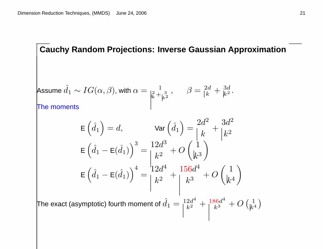
Cauchy Random Projections: Inverse Gaussian Approximation

Assume d1 ∼ IG(α, β), with α = 12

k+ 3

k2

, β = 2dk + 3d

k2 .

The moments

E(

d1

)

= d, Var(

d1

)

=2d2

k+

3d2

k2

E(

d1 − E(d1))3

=12d3

k2+ O

(

1

k3

)

E(

d1 − E(d1))4

=12d4

k2+

156d4

k3+ O

(

1

k4

)

The exact (asymptotic) fourth moment of d1 = 12d4

k2 + 186d4

k3 + O(

1k4

)


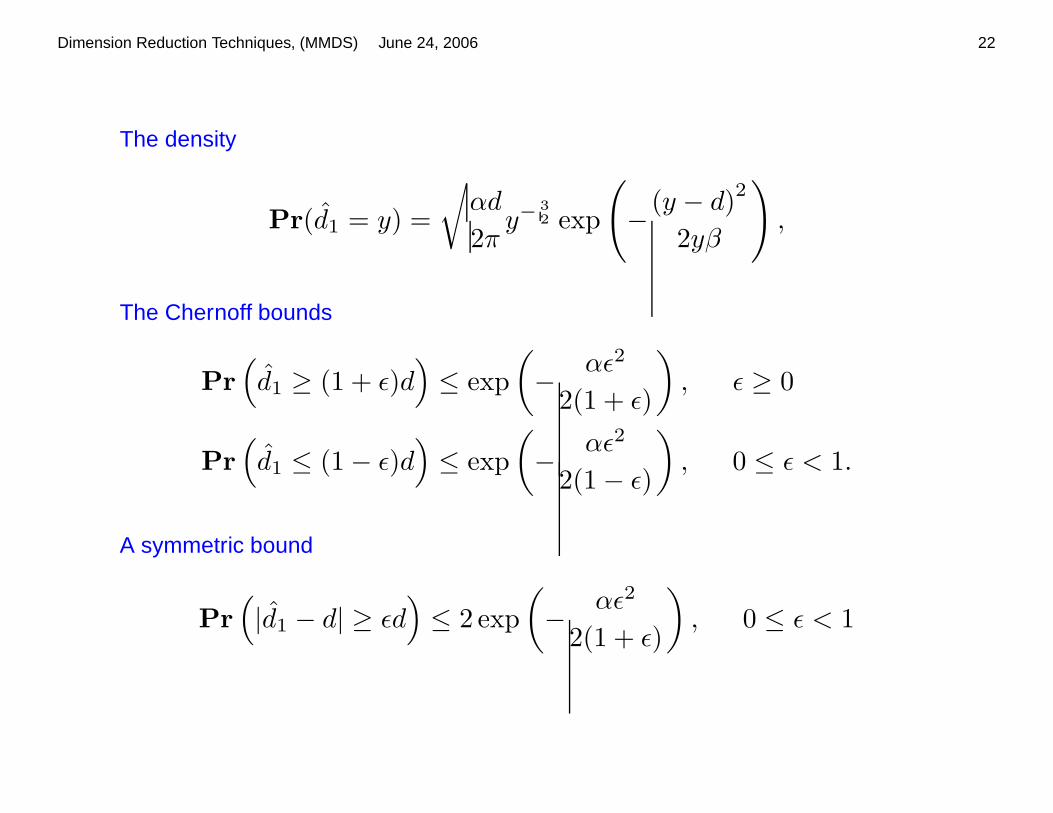
The density

Pr(d1 = y) =

√

αd

2πy− 3

2 exp

(

−(y − d)

2

2yβ

)

,

The Chernoff bounds

Pr

(

d1 ≥ (1 + ε)d)

≤ exp

(

−αε2

2(1 + ε)

)

, ε ≥ 0

Pr

(

d1 ≤ (1 − ε)d)

≤ exp

(

−αε2

2(1 − ε)

)

, 0 ≤ ε < 1.

A symmetric bound

Pr

(

|d1 − d| ≥ εd)

≤ 2 exp

(

−αε2

2(1 + ε)

)

, 0 ≤ ε < 1


A JL-type of Bound (Derived by approximation, verified by simulations)

A JL-type of bound follows by letting Pr

(

|d1 − d| > εd)

≤ ξ/ν,

k ≥4.4 (log 2ν − log ξ)

ε2/(1 + ε).

This holds at least for ξ/ν ≥ 10−10, verified by simulations.

(Why the 95% normal quantile = 1.645?)


Cauchy Random Projections: Simulations

Tail probability Pr

(

|d1 − d| > εd)

0 0.2 0.4 0.6 0.8 110

−10

10−8

10−6

10−4

10−2

100

ε

Tai

l pro

babi

lity

Empirical

IG

k=10

k=20k=50k=100

k=200

k=400

The inverse Gaussian approximation is remarkably accurate.


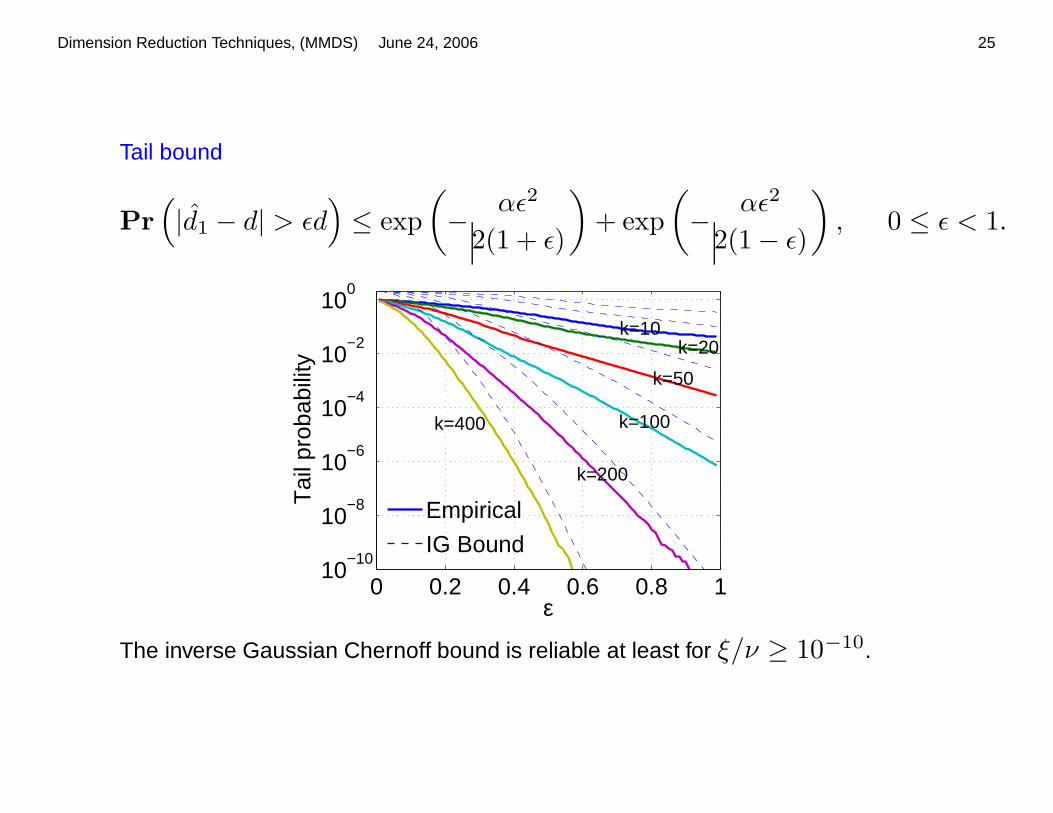
Tail bound

Pr

(

|d1 − d| > εd)

≤ exp

(

−αε2

2(1 + ε)

)

+ exp

(

−αε2

2(1 − ε)

)

, 0 ≤ ε < 1.

0 0.2 0.4 0.6 0.8 110

−10

10−8

10−6

10−4

10−2

100

ε

Tai

l pro

babi

lity

Empirical

IG Bound

k=200

k=100

k=50

k=20k=10

k=400

The inverse Gaussian Chernoff bound is reliable at least for ξ/ν ≥ 10−10.


A Case Study on Microarray Data

Harvard Dataset (PNAS 2001, thank Wing H. Wong): 176 specimen, 3 classes,

12600 genes.

Only 2 (out of 176) specimen were misclassified, by a 5-nearest neighbor classifer

using l1 distances in 12600 dimensions.

Using Cauchy random projections and both nonlinear estimators, the dimension

can be reduced from 12600 to 100, with little loss in accuracy.

Two error measures:

• Median (among 176 × 175/2 = 15488 pairs) absolute errors of estimated

l1 distances, normlized by original median l1 distance.

• Number of misclassifications.


Left: Distance errors Right: Misclassifications

10 1000

0.1

0.2

0.3

0.4

0.5

Sample size k

Ave

rage

abs

olut

e er

ror

GM

MLE

10 1000

5

10

15

20

25

30

Sample size k

Ave

rage

mis

clas

sific

atio

ns

GMMLE

• When k = 100, relative absolute distance error about 10%.

• When k = 100, number of misclassifications < 5.

• MLE is about 10% better than GM (unbiased estimator) in distance errors, as

expected.

• MLE is about 5% − 10% better than GM in misclassifications.


Summary for Cauchy Random Projections

• Linear projections + linear estimators do not work well (impossibility results).

• Linear projections + nonlinear estimators are available and suffice for many

applications (e.g., clustering, SVM kernels, information retrieval).

• Analog of JL bound in l1 exists (in a sense), proved using an unbiased

nonlinear estimator

• The MLE is even better. Highly accurate and

convenient closed-form approximations of the tail bounds are practically useful.

So far so good...


Limitations of Random Projections

• Designed for specific summary statistics (l1 or l2)

• Limited to two-way (pairwise) distances

What about sampling?

• Suitable for any norm and multi-way

• Most samples are zeros, in sparse data

• Possibly large errors in heavy-tailed data

Conditional Random Sampling (CRS): A sketch-based sampling algorithm.

Directly exploit data sparsity


Conditional Random Sampling (CRS): A Global View

Sparse Data Matrix Random Permutation on Columns

12345n

1 2 3 4 5 6 7 8 D12345n

1 2 3 4 5 6 7 8 D

Postings (Non-zero Entries) Sketches (Front of Postings)

12345n

12345n


Conditional Random Sampling (CRS): An Example

Random Sampling on Data Matrix A: If columns are random, first Ds = 10

columns constitute a random sample.

1

2

u

u

1 2 3 4 5 6 7 8 9 10 11 12 13 14 15 16

1 4 0 0 1 2 0 1 0 0 3 0 0 2 1 1

0 3 0 2 0 1 0 0 1 2 1 0 1 0 2 0

Postings P: Only store non-zeros, “ID (Value),” sorted ascending by the IDs.

21P : 2 (3) 4 (2) 6 (1) 9 (1) 10 (2) 11 (1) 13 (1) 15 (2)

P : 1 (1) 2 (4) 5 (1) 6 (2) 8 (1) 11 (3) 14 (2) 15 (1) 16(1)

Sketches K: A sketch, Ki, of postings Pi, is the first ki entries of Pi. Suppose

k1 = 5, k2 = 6.

21K : 2 (3) 4 (2) 6 (1) 9 (1) 10 (2)

K : 1 (1) 2 (4) 5 (1) 6 (2) 8 (1) 11 (3)

What if remove the entry 11(3)?... We get random samples.


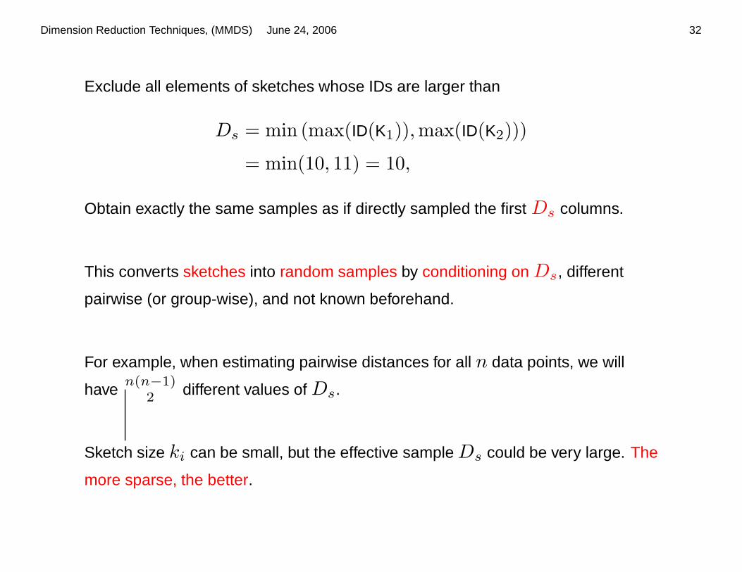
Exclude all elements of sketches whose IDs are larger than

Ds = min (max(ID(K1)), max(ID(K2)))

= min(10, 11) = 10,

Obtain exactly the same samples as if directly sampled the first Ds columns.

This converts sketches into random samples by conditioning on Ds, different

pairwise (or group-wise), and not known beforehand.

For example, when estimating pairwise distances for all n data points, we will

haven(n−1)

2 different values of Ds.

Sketch size ki can be small, but the effective sample Ds could be very large. The

more sparse, the better.


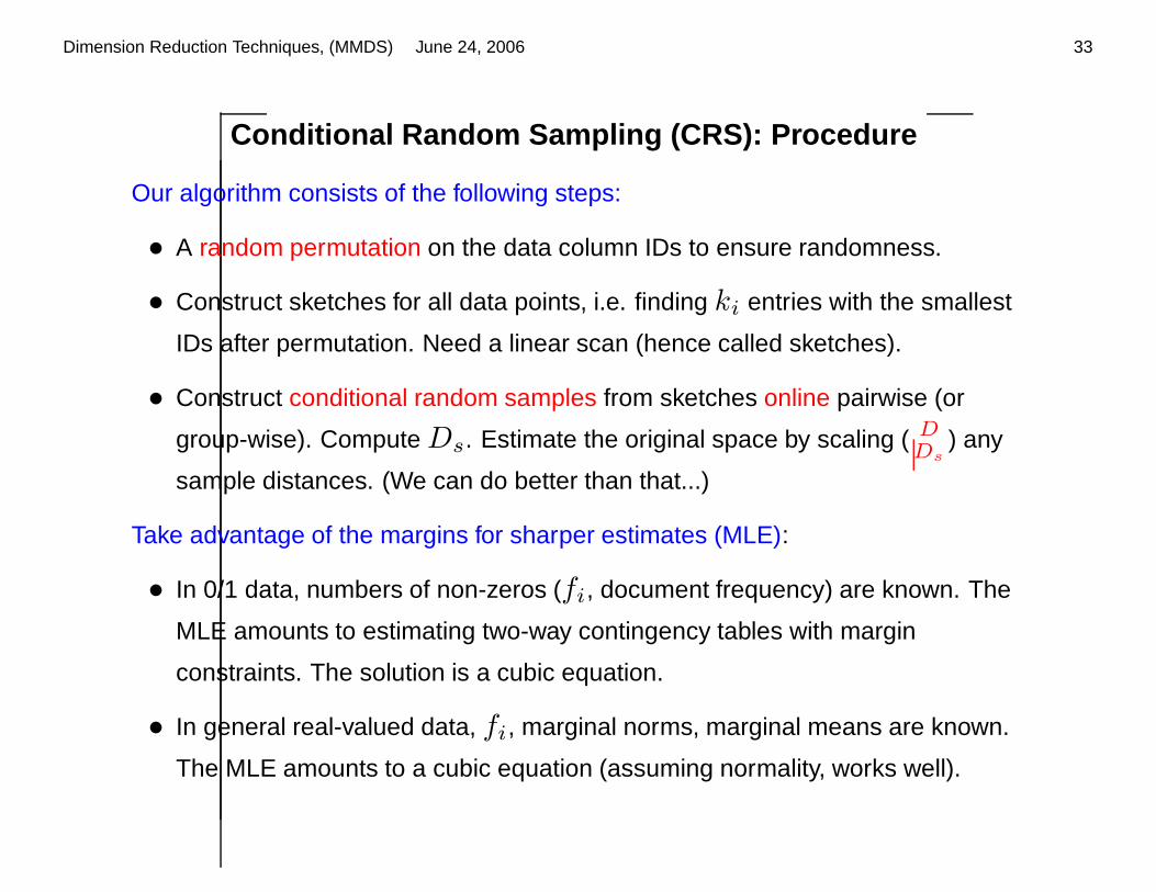
Conditional Random Sampling (CRS): Procedure

Our algorithm consists of the following steps:

• A random permutation on the data column IDs to ensure randomness.

• Construct sketches for all data points, i.e. finding ki entries with the smallest

IDs after permutation. Need a linear scan (hence called sketches).

• Construct conditional random samples from sketches online pairwise (or

group-wise). Compute Ds. Estimate the original space by scaling ( DDs

) any

sample distances. (We can do better than that...)

Take advantage of the margins for sharper estimates (MLE):

• In 0/1 data, numbers of non-zeros (fi, document frequency) are known. The

MLE amounts to estimating two-way contingency tables with margin

constraints. The solution is a cubic equation.

• In general real-valued data, fi, marginal norms, marginal means are known.

The MLE amounts to a cubic equation (assuming normality, works well).


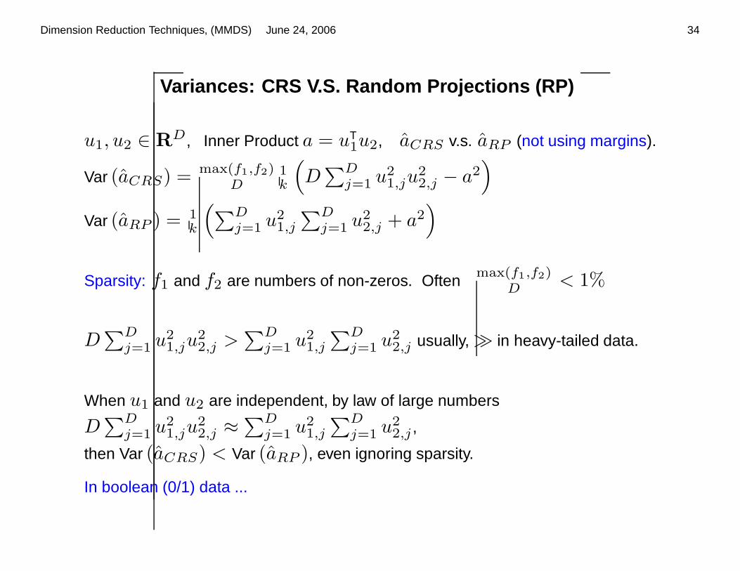
Variances: CRS V.S. Random Projections (RP)

u1, u2 ∈ RD, Inner Product a = uT

1u2, aCRS v.s. aRP (not using margins).

Var (aCRS) = max(f1,f2)D

1k

(

D∑D

j=1 u21,ju

22,j − a2

)

Var (aRP ) = 1k

(

∑Dj=1 u2

1,j

∑Dj=1 u2

2,j + a2)

Sparsity: f1 and f2 are numbers of non-zeros. Oftenmax(f1,f2)

D < 1%

D∑D

j=1 u21,ju

22,j >

∑Dj=1 u2

1,j

∑Dj=1 u2

2,j usually, � in heavy-tailed data.

When u1 and u2 are independent, by law of large numbers

D∑D

j=1 u21,ju

22,j ≈

∑Dj=1 u2

1,j

∑Dj=1 u2

2,j ,

then Var (aCRS) < Var (aRP ), even ignoring sparsity.

In boolean (0/1) data ...


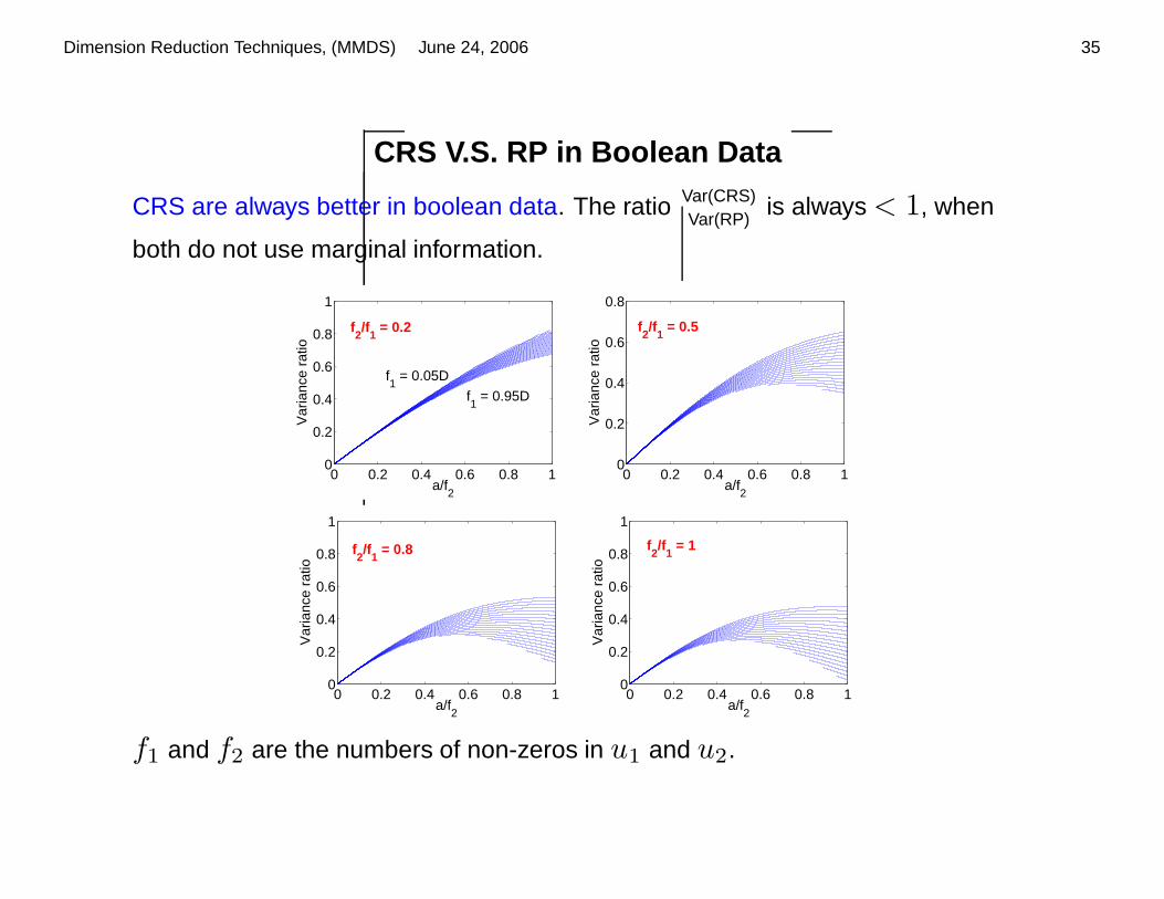
CRS V.S. RP in Boolean Data

CRS are always better in boolean data. The ratio Var(CRS)Var(RP)

is always < 1, when

both do not use marginal information.

0 0.2 0.4 0.6 0.8 10

0.2

0.4

0.6

0.8

1

a/f2

Var

ianc

e ra

tio

f2/f

1 = 0.2

f1 = 0.05D

f1 = 0.95D

0 0.2 0.4 0.6 0.8 10

0.2

0.4

0.6

0.8

a/f2

Var

ianc

e ra

tio

f2/f

1 = 0.5

0 0.2 0.4 0.6 0.8 10

0.2

0.4

0.6

0.8

1

a/f2

Var

ianc

e ra

tio

f2/f

1 = 0.8

0 0.2 0.4 0.6 0.8 10

0.2

0.4

0.6

0.8

1

a/f2

Var

ianc

e ra

tio

f2/f

1 = 1

f1 and f2 are the numbers of non-zeros in u1 and u2.


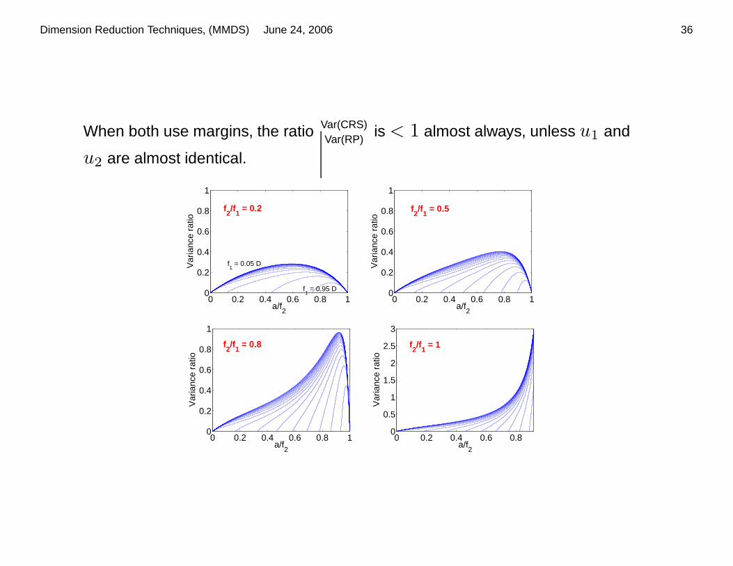
When both use margins, the ratio Var(CRS)Var(RP)

is < 1 almost always, unless u1 and

u2 are almost identical.

0 0.2 0.4 0.6 0.8 10

0.2

0.4

0.6

0.8

1

a/f2

Var

ianc

e ra

tio

f2/f

1 = 0.2

f1 = 0.05 D

f1 = 0.95 D

0 0.2 0.4 0.6 0.8 10

0.2

0.4

0.6

0.8

1

a/f2

Var

ianc

e ra

tio

f2/f

1 = 0.5

0 0.2 0.4 0.6 0.8 10

0.2

0.4

0.6

0.8

1

a/f2

Var

ianc

e ra

tio

f2/f

1 = 0.8

0 0.2 0.4 0.6 0.80

0.5

1

1.5

2

2.5

3

a/f2

Var

ianc

e ra

tio

f2/f

1 = 1


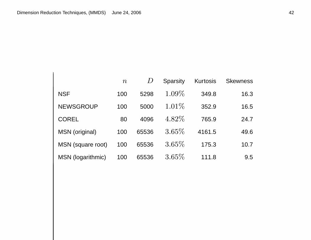
Empirical Evaluations of CRS and RP

Data (Each has totaln(n−1)

2 pairs of distances)

n D Sparsity Kurtosis Skewness

NSF 100 5298 1.09% 349.8 16.3

NEWSGROUP 100 5000 1.01% 352.9 16.5

COREL 80 4096 4.82% 765.9 24.7

MSN (original) 100 65536 3.65% 4161.5 49.6

MSN (square root) 100 65536 3.65% 175.3 10.7

MSN (logarithmic) 100 65536 3.65% 111.8 9.5

• NEWSGROUP and NSF (thank Bingham and Dhillon): document distance

• COREL: Image histogram distance

• MSN : Word distance,

• Median sample kurtosis and skewness, (heavy-tailed, highly-skewed)


Variable sketch size for CRS

We could adjust sketch sizes according to data sparsity. Sample more from the

more frequent ones.

Evaluation metric

Among then(n−1)

2 pairs, the percentage for which CRS does better than random

projections. Want > 0.5

Results...


NSF Data: Conditional Random Sampling (CRS) is overwhelmingly better than

Random Projections (RP).

10 20 30 40 500.9985

0.999

0.9995

1

Sample size k

Per

cent

age Inner product

10 20 30 40 500.94

0.96

0.98

1

Sample size k

L1 distance

10 20 30 40 500.2

0.4

0.6

0.8

1

Sample size k

L2 distance

10 20 30 40 50

0.9994

0.9996

0.9998

1

Sample size k

L2 distance (Margins)

Dashed: Fixed sample size, Solid: Variable sketch size


NEWSGROUP Data: CRS is overwhelmingly better than RP.

10 20 300.985

0.99

0.995

1

Sample size k

Per

cent

age Inner product

10 20 300.9

0.95

1

Sample size k

L1 distance

10 20 300.2

0.4

0.6

0.8

1

Sample size k

L2 distance

10 20 300.99

0.995

1

Sample size k



COREL Image Data: CRS are still better than RP for inner product and l2

distance (using margins)

10 20 30 40 500.75

0.8

0.85

0.9

Sample size k

Per

cent

age

Inner product

10 20 30 40 500

0.01

0.02

0.03

0.04

Sample size k

L1 distance

10 20 30 40 50−0.1

−0.05

0

0.05

0.1

Sample size k

L2 distance

10 20 30 40 500.5

0.6

0.7

0.8

0.9

Sample size k



n D Sparsity Kurtosis Skewness

NSF 100 5298 1.09% 349.8 16.3

NEWSGROUP 100 5000 1.01% 352.9 16.5

COREL 80 4096 4.82% 765.9 24.7

MSN (original) 100 65536 3.65% 4161.5 49.6

MSN (square root) 100 65536 3.65% 175.3 10.7

MSN (logarithmic) 100 65536 3.65% 111.8 9.5


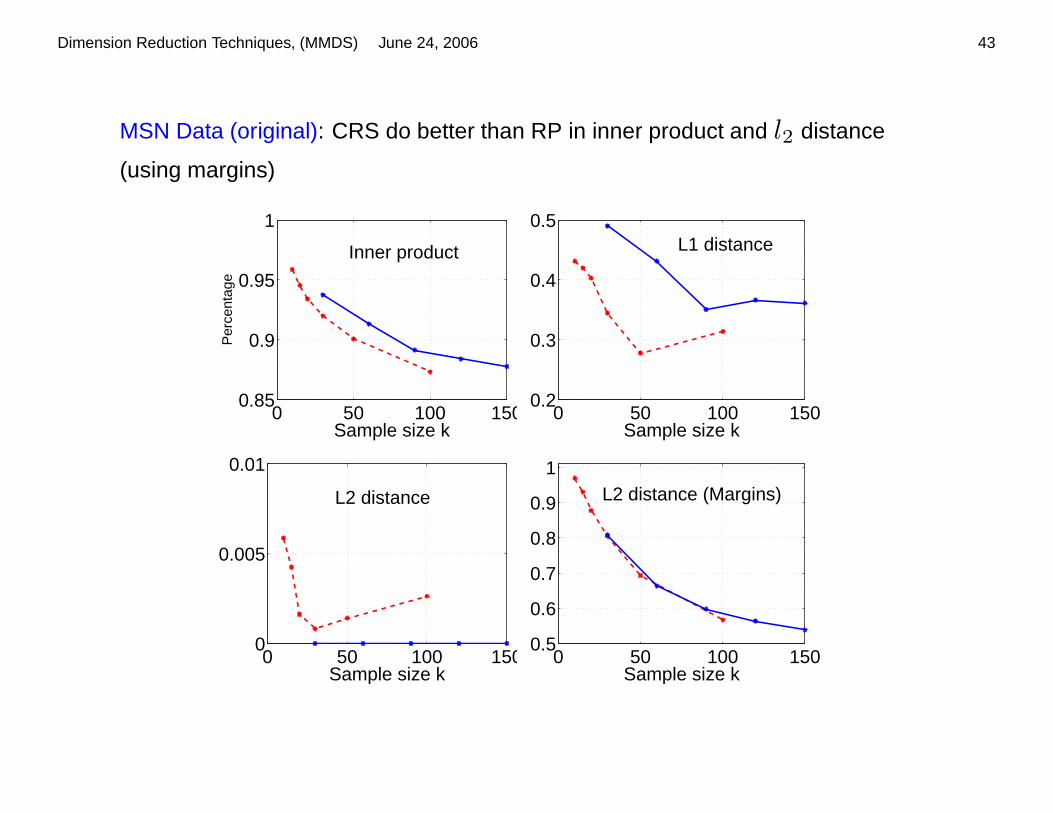
MSN Data (original): CRS do better than RP in inner product and l2 distance

(using margins)

0 50 100 1500.85

0.9

0.95

1

Sample size k

Per

cent

age

Inner product

0 50 100 1500.2

0.3

0.4

0.5

Sample size k

L1 distance

0 50 100 1500

0.005

0.01

Sample size k

L2 distance

0 50 100 1500.5

0.6

0.7

0.8

0.9

1

Sample size k



MSN Data (square root): After transformation (as in practice), CRS do better than

RP in inner product, l1 and l2 (using margins)

0 50 100 1500.92

0.94

0.96

0.98

1

Sample size k

Per

cent

age Inner product

0 50 100 1500.92

0.94

0.96

0.98

1

Sample size k

L1 distance

0 50 100 1500.3

0.35

0.4

0.45

Sample size k

L2 distance

0 50 100 1500.94

0.96

0.98

1

Sample size k



Summary of the Empirical Comparisons

Conditional Random Sampling (CRS) v.s. Random Projections (RP)

• CRS are particularly well-suited for inner products.

• CRS are often comparable to Cauchy random projections for l1 distances.

• Using the margins, CRS are also effectively for l2 distances.

• Can adjust the sketch size according to the data sparsity, which in general

improves the overall performance.

• Using a fixed sketch size, then the less freqent (but often more interesting)

items are emphasized.


Conclusions• Too much data (although never enough)

• Compact data representations

• Accurate approximation algorithms (estimators)

• Dimension Reduction Techniques (in addition to SVD)

• Random sampling

• Sketching (e.g., normal and Cauchy random projections)

• Conditional Random Sampling (sampling + sketching)

• Improve normal random projection (for l2) using margins by nonlinear MLE.

• Propose nonlinear estimators for Cauchy random projections for l1.

• Conditional Random Sampling (CRS), for sparse data and 0/1 data

• Flexible (can adjust sample size according to sparsity)

• Good for estimating inner products

• Easy to take advantage of margins.


References

Ping Li, Trevor Hastie, and Kenneth Church,

Practical Procedurs for Dimension Reduction in l1,

Tech. report, Stanford Statistics, 2006

http://www.stanford.edu/˜pingli98/publications/cauchy_rp_tr.pdf

Ping Li, Kenneth Church, and Trevor Hastie,

Conditional Random Sampling: A Sketch-based Sampling Technique for Sparse

Data,

Tech. report, Stanford Statistics, 2006

http://www.stanford.edu/˜pingli98/publications/CRS_tr.pdf

dimension reduction techniques - stanford...

Documents