mmds ch2.2-2.2.3 - the stanford university infolabinfolab.stanford.edu/~ullman/mmds/ch2.pdf ·...
TRANSCRIPT

20
Chapter 2
MapReduce and the New
Software Stack
Modern data-mining applications, often called “big-data” analysis, require usto manage immense amounts of data quickly. In many of these applications, thedata is extremely regular, and there is ample opportunity to exploit parallelism.Important examples are:
1. The ranking of Web pages by importance, which involves an iteratedmatrix-vector multiplication where the dimension is many billions.
2. Searches in “friends” networks at social-networking sites, which involvegraphs with hundreds of millions of nodes and many billions of edges.
To deal with applications such as these, a new software stack has evolved. Theseprogramming systems are designed to get their parallelism not from a “super-computer,” but from “computing clusters” – large collections of commodityhardware, including conventional processors (“compute nodes”) connected byEthernet cables or inexpensive switches. The software stack begins with a newform of file system, called a “distributed file system,” which features much largerunits than the disk blocks in a conventional operating system. Distributed filesystems also provide replication of data or redundancy to protect against thefrequent media failures that occur when data is distributed over thousands oflow-cost compute nodes.
On top of these file systems, many different higher-level programming sys-tems have been developed. Central to the new software stack is a programmingsystem called MapReduce. Implementations of MapReduce enable many of themost common calculations on large-scale data to be performed on computingclusters efficiently and in a way that is tolerant of hardware failures during thecomputation.
MapReduce systems are evolving and extending rapidly. Today, it is com-mon for MapReduce programs to be created from still higher-level programming
21
22 CHAPTER 2. MAPREDUCE AND THE NEW SOFTWARE STACK
systems, often an implementation of SQL. Further, MapReduce turns out to bea useful, but simple, case of more general and powerful ideas. We includein this chapter a discussion of generalizations of MapReduce, first to systemsthat support acyclic workflows and then to systems that implement recursivealgorithms.
Our last topic for this chapter is the design of good MapReduce algorithms,a subject that often differs significantly from the matter of designing goodparallel algorithms to be run on a supercomputer. When designing MapReducealgorithms, we often find that the greatest cost is in the communication. Wethus investigate communication cost and what it tells us about the most efficientMapReduce algorithms. For several common applications of MapReduce we areable to give families of algorithms that optimally trade the communication costagainst the degree of parallelism.
2.1 Distributed File Systems
Most computing is done on a single processor, with its main memory, cache, andlocal disk (a compute node). In the past, applications that called for parallelprocessing, such as large scientific calculations, were done on special-purposeparallel computers with many processors and specialized hardware. However,the prevalence of large-scale Web services has caused more and more computingto be done on installations with thousands of compute nodes operating moreor less independently. In these installations, the compute nodes are commodityhardware, which greatly reduces the cost compared with special-purpose parallelmachines.
These new computing facilities have given rise to a new generation of pro-gramming systems. These systems take advantage of the power of parallelismand at the same time avoid the reliability problems that arise when the comput-ing hardware consists of thousands of independent components, any of whichcould fail at any time. In this section, we discuss both the characteristics ofthese computing installations and the specialized file systems that have beendeveloped to take advantage of them.
2.1.1 Physical Organization of Compute Nodes
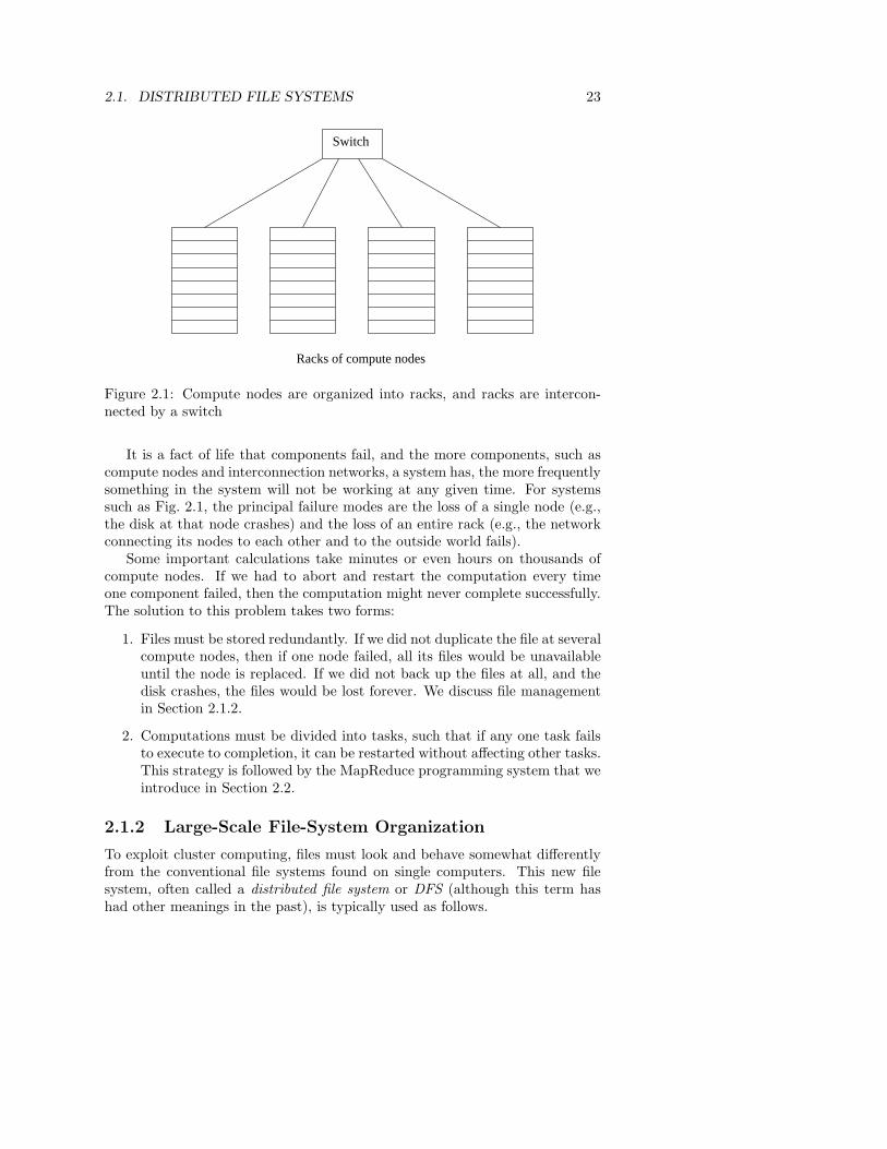
The new parallel-computing architecture, sometimes called cluster computing,is organized as follows. Compute nodes are stored on racks, perhaps 8–64on a rack. The nodes on a single rack are connected by a network, typicallygigabit Ethernet. There can be many racks of compute nodes, and racks areconnected by another level of network or a switch. The bandwidth of inter-rackcommunication is somewhat greater than the intrarack Ethernet, but given thenumber of pairs of nodes that might need to communicate between racks, thisbandwidth may be essential. Figure 2.1 suggests the architecture of a large-scale computing system. However, there may be many more racks and manymore compute nodes per rack.
2.1. DISTRIBUTED FILE SYSTEMS 23
Switch
Racks of compute nodes
Figure 2.1: Compute nodes are organized into racks, and racks are intercon-nected by a switch
It is a fact of life that components fail, and the more components, such ascompute nodes and interconnection networks, a system has, the more frequentlysomething in the system will not be working at any given time. For systemssuch as Fig. 2.1, the principal failure modes are the loss of a single node (e.g.,the disk at that node crashes) and the loss of an entire rack (e.g., the networkconnecting its nodes to each other and to the outside world fails).
Some important calculations take minutes or even hours on thousands ofcompute nodes. If we had to abort and restart the computation every timeone component failed, then the computation might never complete successfully.The solution to this problem takes two forms:
1. Files must be stored redundantly. If we did not duplicate the file at severalcompute nodes, then if one node failed, all its files would be unavailableuntil the node is replaced. If we did not back up the files at all, and thedisk crashes, the files would be lost forever. We discuss file managementin Section 2.1.2.
2. Computations must be divided into tasks, such that if any one task failsto execute to completion, it can be restarted without affecting other tasks.This strategy is followed by the MapReduce programming system that weintroduce in Section 2.2.
2.1.2 Large-Scale File-System Organization
To exploit cluster computing, files must look and behave somewhat differentlyfrom the conventional file systems found on single computers. This new filesystem, often called a distributed file system or DFS (although this term hashad other meanings in the past), is typically used as follows.
24 CHAPTER 2. MAPREDUCE AND THE NEW SOFTWARE STACK
DFS Implementations
There are several distributed file systems of the type we have describedthat are used in practice. Among these:
1. The Google File System (GFS), the original of the class.
2. Hadoop Distributed File System (HDFS), an open-source DFS usedwith Hadoop, an implementation of MapReduce (see Section 2.2)and distributed by the Apache Software Foundation.
3. CloudStore, an open-source DFS originally developed by Kosmix.
• Files can be enormous, possibly a terabyte in size. If you have only smallfiles, there is no point using a DFS for them.
• Files are rarely updated. Rather, they are read as data for some calcula-tion, and possibly additional data is appended to files from time to time.For example, an airline reservation system would not be suitable for aDFS, even if the data were very large, because the data is changed sofrequently.
Files are divided into chunks, which are typically 64 megabytes in size.Chunks are replicated, perhaps three times, at three different compute nodes.Moreover, the nodes holding copies of one chunk should be located on differentracks, so we don’t lose all copies due to a rack failure. Normally, both the chunksize and the degree of replication can be decided by the user.
To find the chunks of a file, there is another small file called the master nodeor name node for that file. The master node is itself replicated, and a directoryfor the file system as a whole knows where to find its copies. The directory itselfcan be replicated, and all participants using the DFS know where the directorycopies are.
2.2 MapReduce
MapReduce is a style of computing that has been implemented in several sys-tems, including Google’s internal implementation (simply called MapReduce)and the popular open-source implementation Hadoop which can be obtained,along with the HDFS file system from the Apache Foundation. You can usean implementation of MapReduce to manage many large-scale computationsin a way that is tolerant of hardware faults. All you need to write are twofunctions, called Map and Reduce, while the system manages the parallel exe-cution, coordination of tasks that execute Map or Reduce, and also deals with
2.2. MAPREDUCE 25
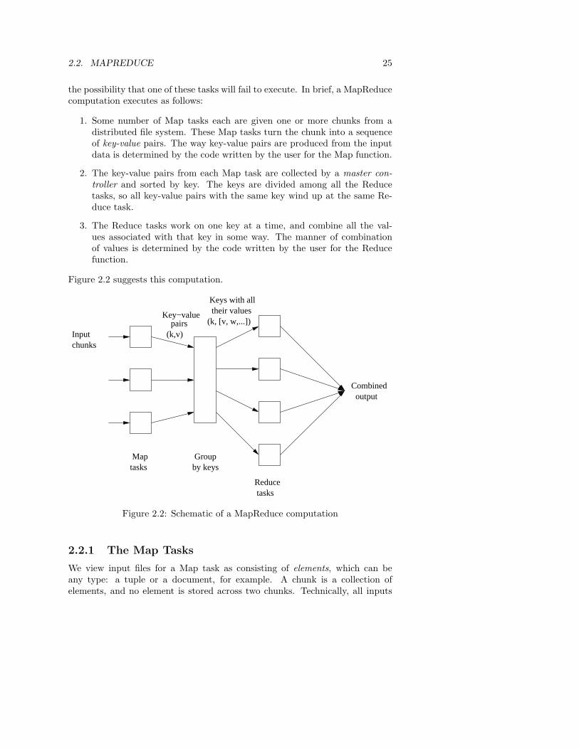
the possibility that one of these tasks will fail to execute. In brief, a MapReducecomputation executes as follows:
1. Some number of Map tasks each are given one or more chunks from adistributed file system. These Map tasks turn the chunk into a sequenceof key-value pairs. The way key-value pairs are produced from the inputdata is determined by the code written by the user for the Map function.
2. The key-value pairs from each Map task are collected by a master con-troller and sorted by key. The keys are divided among all the Reducetasks, so all key-value pairs with the same key wind up at the same Re-duce task.
3. The Reduce tasks work on one key at a time, and combine all the val-ues associated with that key in some way. The manner of combinationof values is determined by the code written by the user for the Reducefunction.
Figure 2.2 suggests this computation.
Inputchunks
Groupby keys
Key−value
(k,v)pairs
their valuesKeys with all
outputCombined
Maptasks
Reducetasks
(k, [v, w,...])
Figure 2.2: Schematic of a MapReduce computation
2.2.1 The Map Tasks
We view input files for a Map task as consisting of elements, which can beany type: a tuple or a document, for example. A chunk is a collection ofelements, and no element is stored across two chunks. Technically, all inputs
26 CHAPTER 2. MAPREDUCE AND THE NEW SOFTWARE STACK
to Map tasks and outputs from Reduce tasks are of the key-value-pair form,but normally the keys of input elements are not relevant and we shall tend toignore them. Insisting on this form for inputs and outputs is motivated by thedesire to allow composition of several MapReduce processes.
The Map function takes an input element as its argument and produceszero or more key-value pairs. The types of keys and values are each arbitrary.Further, keys are not “keys” in the usual sense; they do not have to be unique.Rather a Map task can produce several key-value pairs with the same key, evenfrom the same element.
Example 2.1 : We shall illustrate a MapReduce computation with what hasbecome the standard example application: counting the number of occurrencesfor each word in a collection of documents. In this example, the input file is arepository of documents, and each document is an element. The Map functionfor this example uses keys that are of type String (the words) and values thatare integers. The Map task reads a document and breaks it into its sequenceof words w1, w2, . . . , wn. It then emits a sequence of key-value pairs where thevalue is always 1. That is, the output of the Map task for this document is thesequence of key-value pairs:
(w1, 1), (w2, 1), . . . , (wn, 1)
Note that a single Map task will typically process many documents – allthe documents in one or more chunks. Thus, its output will be more than thesequence for the one document suggested above. Note also that if a word wappears m times among all the documents assigned to that process, then therewill be m key-value pairs (w, 1) among its output. An option, which we discussin Section 2.2.4, is to combine these m pairs into a single pair (w, m), but wecan only do that because, as we shall see, the Reduce tasks apply an associativeand commutative operation, addition, to the values. 2
2.2.2 Grouping by Key
As soon as the Map tasks have all completed successfully, the key-value pairs aregrouped by key, and the values associated with each key are formed into a list ofvalues. The grouping is performed by the system, regardless of what the Mapand Reduce tasks do. The master controller process knows how many Reducetasks there will be, say r such tasks. The user typically tells the MapReducesystem what r should be. Then the master controller picks a hash function thatapplies to keys and produces a bucket number from 0 to r − 1. Each key thatis output by a Map task is hashed and its key-value pair is put in one of r localfiles. Each file is destined for one of the Reduce tasks.1
1Optionally, users can specify their own hash function or other method for assigning keys
to Reduce tasks. However, whatever algorithm is used, each key is assigned to one and only
one Reduce task.
2.2. MAPREDUCE 27
To perform the grouping by key and distribution to the Reduce tasks, themaster controller merges the files from each Map task that are destined fora particular Reduce task and feeds the merged file to that process as a se-quence of key-list-of-value pairs. That is, for each key k, the input to theReduce task that handles key k is a pair of the form (k, [v1, v2, . . . , vn]), where(k, v1), (k, v2), . . . , (k, vn) are all the key-value pairs with key k coming fromall the Map tasks.
2.2.3 The Reduce Tasks
The Reduce function’s argument is a pair consisting of a key and its list ofassociated values. The output of the Reduce function is a sequence of zero ormore key-value pairs. These key-value pairs can be of a type different fromthose sent from Map tasks to Reduce tasks, but often they are the same type.We shall refer to the application of the Reduce function to a single key and itsassociated list of values as a reducer.
A Reduce task receives one or more keys and their associated value lists.That is, a Reduce task executes one or more reducers. The outputs from all theReduce tasks are merged into a single file. Reducers may be partitioned amonga smaller number of Reduce tasks is by hashing the keys and associating eachReduce task with one of the buckets of the hash function.
Example 2.2 : Let us continue with the word-count example of Example 2.1.The Reduce function simply adds up all the values. The output of a reducerconsists of the word and the sum. Thus, the output of all the Reduce tasks is asequence of (w, m) pairs, where w is a word that appears at least once amongall the input documents and m is the total number of occurrences of w amongall those documents. 2
2.2.4 Combiners
Sometimes, a Reduce function is associative and commutative. That is, thevalues to be combined can be combined in any order, with the same result.The addition performed in Example 2.2 is an example of an associative andcommutative operation. It doesn’t matter how we group a list of numbersv1, v2, . . . , vn; the sum will be the same.
When the Reduce function is associative and commutative, we can pushsome of what the reducers do to the Map tasks. For example, instead of theMap tasks in Example 2.1 producing many pairs (w, 1), (w, 1), . . ., we couldapply the Reduce function within the Map task, before the output of the Maptasks is subject to grouping and aggregation. These key-value pairs would thusbe replaced by one pair with key w and value equal to the sum of all the 1’s inall those pairs. That is, the pairs with key w generated by a single Map taskwould be replaced by a pair (w, m), where m is the number of times that wappears among the documents handled by this Map task. Note that it is stillnecessary to do grouping and aggregation and to pass the result to the Reduce

28 CHAPTER 2. MAPREDUCE AND THE NEW SOFTWARE STACK
Reducers, Reduce Tasks, Compute Nodes, and Skew
If we want maximum parallelism, then we could use one Reduce taskto execute each reducer, i.e., a single key and its associated value list.Further, we could execute each Reduce task at a different compute node,so they would all execute in parallel. This plan is not usually the best. Oneproblem is that there is overhead associated with each task we create, sowe might want to keep the number of Reduce tasks lower than the numberof different keys. Moreover, often there are far more keys than there arecompute nodes available, so we would get no benefit from a huge numberof Reduce tasks.
Second, there is often significant variation in the lengths of the valuelists for different keys, so different reducers take different amounts of time.If we make each reducer a separate Reduce task, then the tasks themselveswill exhibit skew – a significant difference in the amount of time eachtakes. We can reduce the impact of skew by using fewer Reduce tasksthan there are reducers. If keys are sent randomly to Reduce tasks, wecan expect that there will be some averaging of the total time required bythe different Reduce tasks. We can further reduce the skew by using moreReduce tasks than there are compute nodes. In that way, long Reducetasks might occupy a compute node fully, while several shorter Reducetasks might run sequentially at a single compute node.
tasks, since there will typically be one key-value pair with key w coming fromeach of the Map tasks.
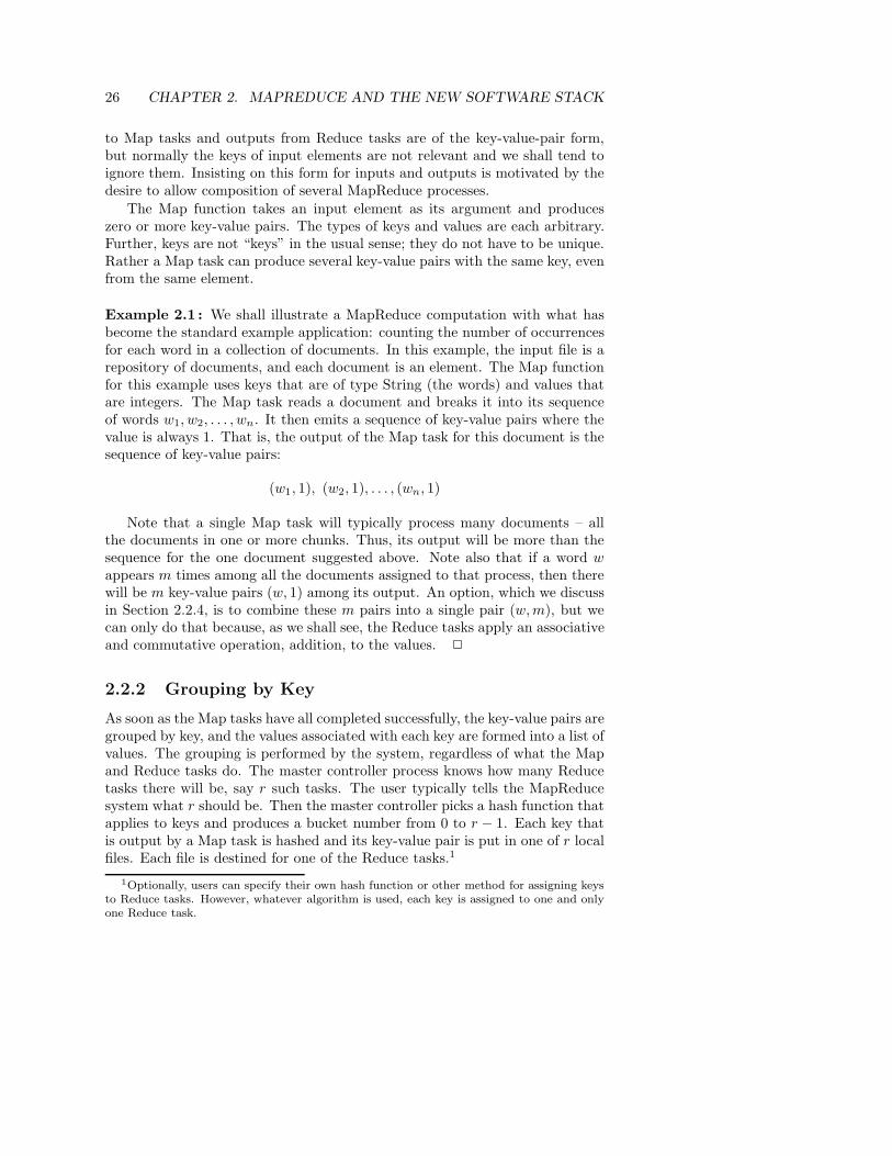
2.2.5 Details of MapReduce Execution
Let us now consider in more detail how a program using MapReduce is executed.Figure 2.3 offers an outline of how processes, tasks, and files interact. Takingadvantage of a library provided by a MapReduce system such as Hadoop, theuser program forks a Master controller process and some number of Workerprocesses at different compute nodes. Normally, a Worker handles either Maptasks (a Map worker) or Reduce tasks (a Reduce worker), but not both.
The Master has many responsibilities. One is to create some number ofMap tasks and some number of Reduce tasks, these numbers being selectedby the user program. These tasks will be assigned to Worker processes by theMaster. It is reasonable to create one Map task for every chunk of the inputfile(s), but we may wish to create fewer Reduce tasks. The reason for limitingthe number of Reduce tasks is that it is necessary for each Map task to createan intermediate file for each Reduce task, and if there are too many Reducetasks the number of intermediate files explodes.
The Master keeps track of the status of each Map and Reduce task (idle,
2.2. MAPREDUCE 29
ProgramUser
Master
Worker
Worker
Worker
Worker
WorkerData
Input
File
Output
fork forkfork
Mapassign assign
Reduce
Intermediate
Files
Figure 2.3: Overview of the execution of a MapReduce program
executing at a particular Worker, or completed). A Worker process reports tothe Master when it finishes a task, and a new task is scheduled by the Masterfor that Worker process.
Each Map task is assigned one or more chunks of the input file(s) andexecutes on it the code written by the user. The Map task creates a file foreach Reduce task on the local disk of the Worker that executes the Map task.The Master is informed of the location and sizes of each of these files, and theReduce task for which each is destined. When a Reduce task is assigned by theMaster to a Worker process, that task is given all the files that form its input.The Reduce task executes code written by the user and writes its output to afile that is part of the surrounding distributed file system.
2.2.6 Coping With Node Failures
The worst thing that can happen is that the compute node at which the Masteris executing fails. In this case, the entire MapReduce job must be restarted.But only this one node can bring the entire process down; other failures will bemanaged by the Master, and the MapReduce job will complete eventually.
Suppose the compute node at which a Map worker resides fails. This fail-ure will be detected by the Master, because it periodically pings the Workerprocesses. All the Map tasks that were assigned to this Worker will have tobe redone, even if they had completed. The reason for redoing completed Map
30 CHAPTER 2. MAPREDUCE AND THE NEW SOFTWARE STACK
tasks is that their output destined for the Reduce tasks resides at that computenode, and is now unavailable to the Reduce tasks. The Master sets the statusof each of these Map tasks to idle and will schedule them on a Worker whenone becomes available. The Master must also inform each Reduce task that thelocation of its input from that Map task has changed.
Dealing with a failure at the node of a Reduce worker is simpler. The Mastersimply sets the status of its currently executing Reduce tasks to idle. Thesewill be rescheduled on another reduce worker later.
2.2.7 Exercises for Section 2.2
Exercise 2.2.1 : Suppose we execute the word-count MapReduce program de-scribed in this section on a large repository such as a copy of the Web. We shalluse 100 Map tasks and some number of Reduce tasks.
(a) Suppose we do not use a combiner at the Map tasks. Do you expect thereto be significant skew in the times taken by the various reducers to processtheir value list? Why or why not?
(b) If we combine the reducers into a small number of Reduce tasks, say 10tasks, at random, do you expect the skew to be significant? What if weinstead combine the reducers into 10,000 Reduce tasks?
! (c) Suppose we do use a combiner at the 100 Map tasks. Do you expect skewto be significant? Why or why not?
2.3 Algorithms Using MapReduce
MapReduce is not a solution to every problem, not even every problem thatprofitably can use many compute nodes operating in parallel. As we mentionedin Section 2.1.2, the entire distributed-file-system milieu makes sense only whenfiles are very large and are rarely updated in place. Thus, we would not expectto use either a DFS or an implementation of MapReduce for managing on-line retail sales, even though a large on-line retailer such as Amazon.com usesthousands of compute nodes when processing requests over the Web. The reasonis that the principal operations on Amazon data involve responding to searchesfor products, recording sales, and so on, processes that involve relatively littlecalculation and that change the database.2 On the other hand, Amazon mightuse MapReduce to perform certain analytic queries on large amounts of data,such as finding for each user those users whose buying patterns were mostsimilar.
The original purpose for which the Google implementation of MapReducewas created was to execute very large matrix-vector multiplications as are
2Remember that even looking at a product you don’t buy causes Amazon to remember
that you looked at it.
2.3. ALGORITHMS USING MAPREDUCE 31
needed in the calculation of PageRank (See Chapter 5). We shall see thatmatrix-vector and matrix-matrix calculations fit nicely into the MapReducestyle of computing. Another important class of operations that can use MapRe-duce effectively are the relational-algebra operations. We shall examine theMapReduce execution of these operations as well.
2.3.1 Matrix-Vector Multiplication by MapReduce
Suppose we have an n×n matrix M , whose element in row i and column j willbe denoted mij . Suppose we also have a vector v of length n, whose jth elementis vj . Then the matrix-vector product is the vector x of length n, whose ithelement xi is given by
xi =
n∑
j=1
mijvj
If n = 100, we do not want to use a DFS or MapReduce for this calculation.But this sort of calculation is at the heart of the ranking of Web pages thatgoes on at search engines, and there, n is in the tens of billions.3 Let us firstassume that n is large, but not so large that vector v cannot fit in main memoryand thus be available to every Map task.
The matrix M and the vector v each will be stored in a file of the DFS. Weassume that the row-column coordinates of each matrix element will be discov-erable, either from its position in the file, or because it is stored with explicitcoordinates, as a triple (i, j, mij). We also assume the position of element vj inthe vector v will be discoverable in the analogous way.
The Map Function: The Map function is written to apply to one element ofM . However, if v is not already read into main memory at the compute nodeexecuting a Map task, then v is first read, in its entirety, and subsequently willbe available to all applications of the Map function performed at this Map task.Each Map task will operate on a chunk of the matrix M . From each matrixelement mij it produces the key-value pair (i, mijvj). Thus, all terms of thesum that make up the component xi of the matrix-vector product will get thesame key, i.
The Reduce Function: The Reduce function simply sums all the values as-sociated with a given key i. The result will be a pair (i, xi).
2.3.2 If the Vector v Cannot Fit in Main Memory
However, it is possible that the vector v is so large that it will not fit in itsentirety in main memory. It is not required that v fit in main memory at acompute node, but if it does not then there will be a very large number of
3The matrix is sparse, with on the average of 10 to 15 nonzero elements per row, since the
matrix represents the links in the Web, with mij nonzero if and only if there is a link from
page j to page i. Note that there is no way we could store a dense matrix whose side was
1010, since it would have 1020 elements.
32 CHAPTER 2. MAPREDUCE AND THE NEW SOFTWARE STACK
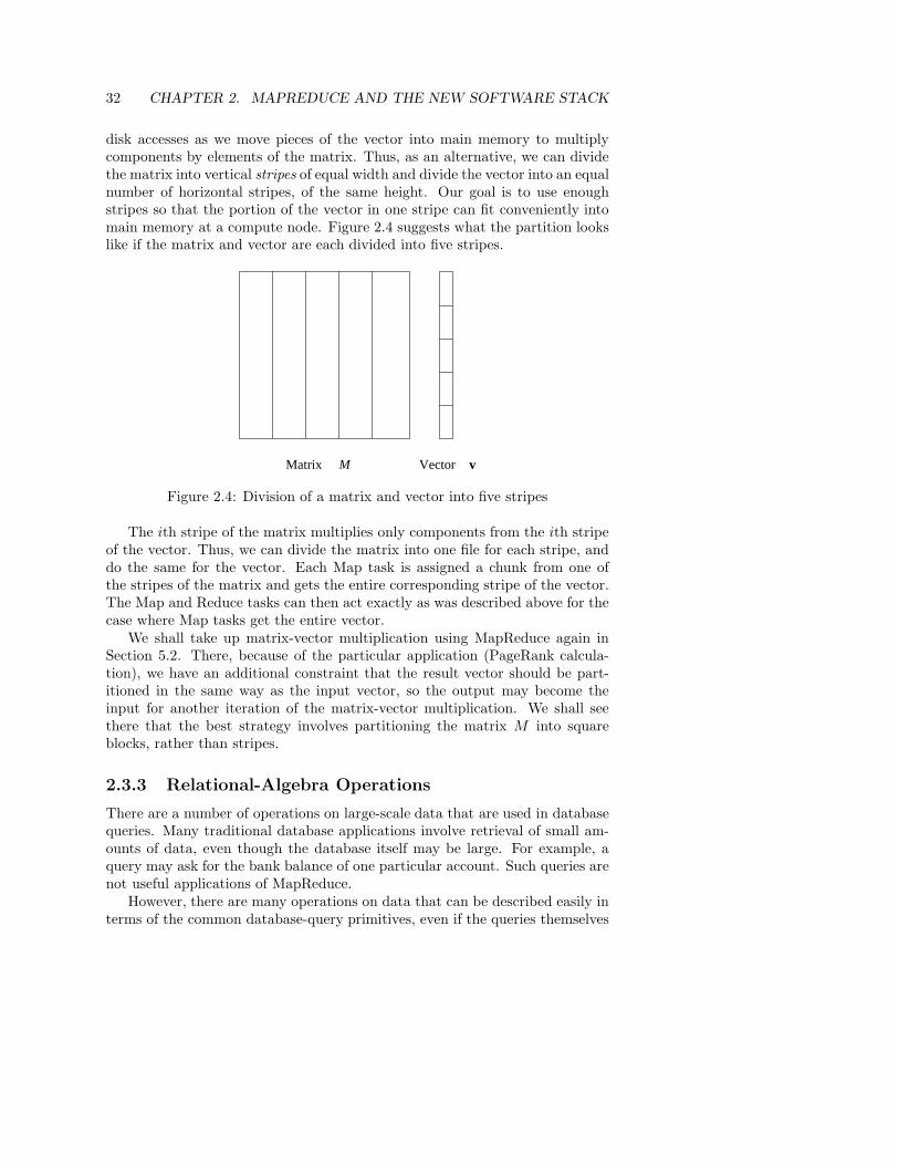
disk accesses as we move pieces of the vector into main memory to multiplycomponents by elements of the matrix. Thus, as an alternative, we can dividethe matrix into vertical stripes of equal width and divide the vector into an equalnumber of horizontal stripes, of the same height. Our goal is to use enoughstripes so that the portion of the vector in one stripe can fit conveniently intomain memory at a compute node. Figure 2.4 suggests what the partition lookslike if the matrix and vector are each divided into five stripes.
MMatrix Vector v
Figure 2.4: Division of a matrix and vector into five stripes
The ith stripe of the matrix multiplies only components from the ith stripeof the vector. Thus, we can divide the matrix into one file for each stripe, anddo the same for the vector. Each Map task is assigned a chunk from one ofthe stripes of the matrix and gets the entire corresponding stripe of the vector.The Map and Reduce tasks can then act exactly as was described above for thecase where Map tasks get the entire vector.
We shall take up matrix-vector multiplication using MapReduce again inSection 5.2. There, because of the particular application (PageRank calcula-tion), we have an additional constraint that the result vector should be part-itioned in the same way as the input vector, so the output may become theinput for another iteration of the matrix-vector multiplication. We shall seethere that the best strategy involves partitioning the matrix M into squareblocks, rather than stripes.
2.3.3 Relational-Algebra Operations
There are a number of operations on large-scale data that are used in databasequeries. Many traditional database applications involve retrieval of small am-ounts of data, even though the database itself may be large. For example, aquery may ask for the bank balance of one particular account. Such queries arenot useful applications of MapReduce.
However, there are many operations on data that can be described easily interms of the common database-query primitives, even if the queries themselves
2.3. ALGORITHMS USING MAPREDUCE 33
are not executed within a database management system. Thus, a good startingpoint for exploring applications of MapReduce is by considering the standardoperations on relations. We assume you are familiar with database systems,the query language SQL, and the relational model, but to review, a relation isa table with column headers called attributes. Rows of the relation are calledtuples. The set of attributes of a relation is called its schema. We often writean expression like R(A1, A2, . . . , An) to say that the relation name is R and itsattributes are A1, A2, . . . , An.
From To
url1 url2
url1 url3
url2 url3
url2 url4
· · · · · ·
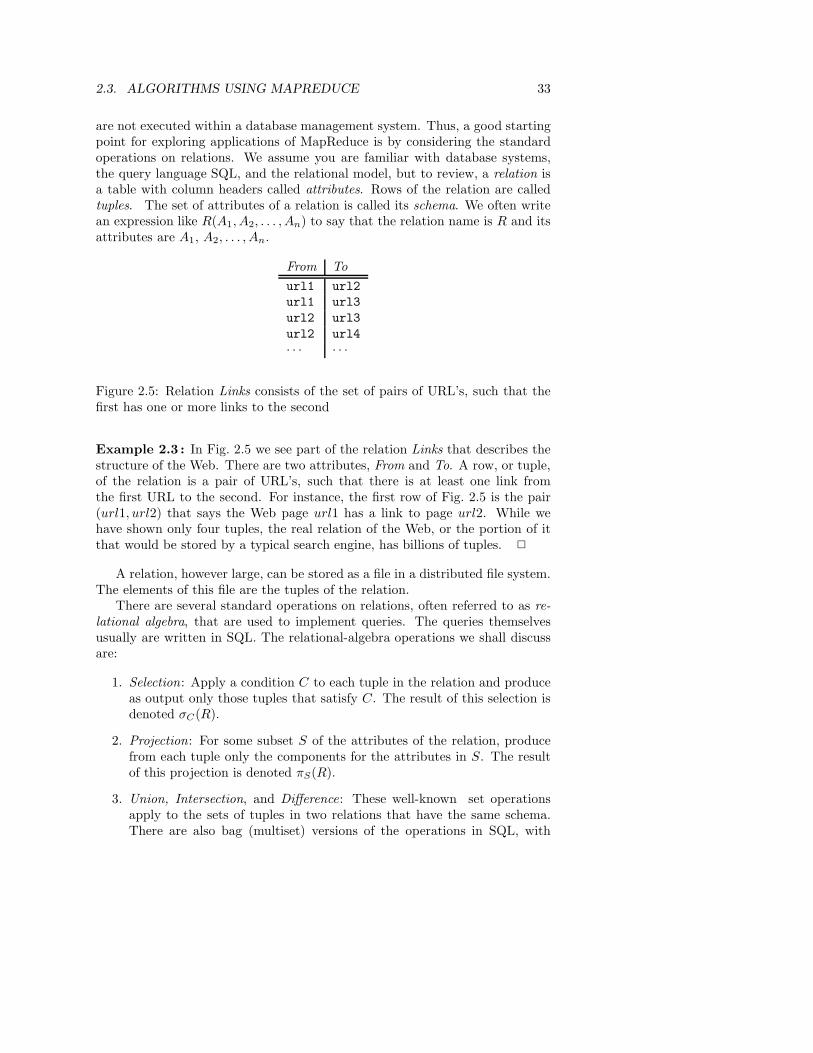
Figure 2.5: Relation Links consists of the set of pairs of URL’s, such that thefirst has one or more links to the second
Example 2.3 : In Fig. 2.5 we see part of the relation Links that describes thestructure of the Web. There are two attributes, From and To. A row, or tuple,of the relation is a pair of URL’s, such that there is at least one link fromthe first URL to the second. For instance, the first row of Fig. 2.5 is the pair(url1, url2) that says the Web page url1 has a link to page url2. While wehave shown only four tuples, the real relation of the Web, or the portion of itthat would be stored by a typical search engine, has billions of tuples. 2
A relation, however large, can be stored as a file in a distributed file system.The elements of this file are the tuples of the relation.
There are several standard operations on relations, often referred to as re-lational algebra, that are used to implement queries. The queries themselvesusually are written in SQL. The relational-algebra operations we shall discussare:
1. Selection: Apply a condition C to each tuple in the relation and produceas output only those tuples that satisfy C. The result of this selection isdenoted σC(R).
2. Projection: For some subset S of the attributes of the relation, producefrom each tuple only the components for the attributes in S. The resultof this projection is denoted πS(R).
3. Union, Intersection, and Difference: These well-known set operationsapply to the sets of tuples in two relations that have the same schema.There are also bag (multiset) versions of the operations in SQL, with
34 CHAPTER 2. MAPREDUCE AND THE NEW SOFTWARE STACK
somewhat unintuitive definitions, but we shall not go into the bag versionsof these operations here.
4. Natural Join: Given two relations, compare each pair of tuples, one fromeach relation. If the tuples agree on all the attributes that are commonto the two schemas, then produce a tuple that has components for eachof the attributes in either schema and agrees with the two tuples on eachattribute. If the tuples disagree on one or more shared attributes, thenproduce nothing from this pair of tuples. The natural join of relations Rand S is denoted R ⊲⊳ S. While we shall discuss executing only the nat-ural join with MapReduce, all equijoins (joins where the tuple-agreementcondition involves equality of attributes from the two relations that do notnecessarily have the same name) can be executed in the same manner. Weshall give an illustration in Example 2.4.
5. Grouping and Aggregation:4 Given a relation R, partition its tuplesaccording to their values in one set of attributes G, called the groupingattributes. Then, for each group, aggregate the values in certain other at-tributes. The normally permitted aggregations are SUM, COUNT, AVG,MIN, and MAX, with the obvious meanings. Note that MIN and MAXrequire that the aggregated attributes have a type that can be compared,e.g., numbers or strings, while SUM and AVG require that the type allowarithmetic operations. We denote a grouping-and-aggregation operationon a relation R by γX(R), where X is a list of elements that are either
(a) A grouping attribute, or
(b) An expression θ(A), where θ is one of the five aggregation opera-tions such as SUM, and A is an attribute not among the groupingattributes.
The result of this operation is one tuple for each group. That tuple hasa component for each of the grouping attributes, with the value commonto tuples of that group. It also has a component for each aggregation,with the aggregated value for that group. We shall see an illustration inExample 2.5.
Example 2.4 : Let us try to find the paths of length two in the Web, usingthe relation Links of Fig. 2.5. That is, we want to find the triples of URL’s(u, v, w) such that there is a link from u to v and a link from v to w. Weessentially want to take the natural join of Links with itself, but we first needto imagine that it is two relations, with different schemas, so we can describe thedesired connection as a natural join. Thus, imagine that there are two copiesof Links, namely L1(U1, U2) and L2(U2, U3). Now, if we compute L1 ⊲⊳ L2,
4Some descriptions of relational algebra do not include these operations, and indeed they
were not part of the original definition of this algebra. However, these operations are so
important in SQL, that modern treatments of relational algebra include them.
2.3. ALGORITHMS USING MAPREDUCE 35
we shall have exactly what we want. That is, for each tuple t1 of L1 (i.e.,each tuple of Links) and each tuple t2 of L2 (another tuple of Links, possiblyeven the same tuple), see if their U2 components are the same. Note thatthese components are the second component of t1 and the first component oft2. If these two components agree, then produce a tuple for the result, withschema (U1, U2, U3). This tuple consists of the first component of t1, thesecond component of t1 (which must equal the first component of t2), and thesecond component of t2.
We may not want the entire path of length two, but only want the pairs(u, w) of URL’s such that there is at least one path from u to w of length two. Ifso, we can project out the middle components by computing πU1,U3(L1 ⊲⊳ L2).2
Example 2.5 : Imagine that a social-networking site has a relation
Friends(User, Friend)
This relation has tuples that are pairs (a, b) such that b is a friend of a. The sitemight want to develop statistics about the number of friends members have.Their first step would be to compute a count of the number of friends of eachuser. This operation can be done by grouping and aggregation, specifically
γUser,COUNT(Friend)(Friends)
This operation groups all the tuples by the value in their first component, sothere is one group for each user. Then, for each group the count of the numberof friends of that user is made. The result will be one tuple for each group, anda typical tuple would look like (Sally, 300), if user “Sally” has 300 friends. 2
2.3.4 Computing Selections by MapReduce
Selections really do not need the full power of MapReduce. They can be donemost conveniently in the map portion alone, although they could also be donein the reduce portion alone. Here is a MapReduce implementation of selectionσC(R).
The Map Function: For each tuple t in R, test if it satisfies C. If so, producethe key-value pair (t, t). That is, both the key and value are t.
The Reduce Function: The Reduce function is the identity. It simply passeseach key-value pair to the output.
Note that the output is not exactly a relation, because it has key-value pairs.However, a relation can be obtained by using only the value components (oronly the key components) of the output.
36 CHAPTER 2. MAPREDUCE AND THE NEW SOFTWARE STACK
2.3.5 Computing Projections by MapReduce
Projection is performed similarly to selection, because projection may causethe same tuple to appear several times, the Reduce function must eliminateduplicates. We may compute πS(R) as follows.
The Map Function: For each tuple t in R, construct a tuple t′ by eliminatingfrom t those components whose attributes are not in S. Output the key-valuepair (t′, t′).
The Reduce Function: For each key t′ produced by any of the Map tasks,there will be one or more key-value pairs (t′, t′). The Reduce function turns(t′, [t′, t′, . . . , t′]) into (t′, t′), so it produces exactly one pair (t′, t′) for this keyt′.
Observe that the Reduce operation is duplicate elimination. This operationis associative and commutative, so a combiner associated with each Map taskcan eliminate whatever duplicates are produced locally. However, the Reducetasks are still needed to eliminate two identical tuples coming from differentMap tasks.
2.3.6 Union, Intersection, and Difference by MapReduce
First, consider the union of two relations. Suppose relations R and S have thesame schema. Map tasks will be assigned chunks from either R or S; it doesn’tmatter which. The Map tasks don’t really do anything except pass their inputtuples as key-value pairs to the Reduce tasks. The latter need only eliminateduplicates as for projection.
The Map Function: Turn each input tuple t into a key-value pair (t, t).
The Reduce Function: Associated with each key t there will be either one ortwo values. Produce output (t, t) in either case.
To compute the intersection, we can use the same Map function. However,the Reduce function must produce a tuple only if both relations have the tuple.If the key t has a list of two values [t, t] associated with it, then the Reducetask for t should produce (t, t). However, if the value-list associated with keyt is just [t], then one of R and S is missing t, so we don’t want to produce atuple for the intersection.
The Map Function: Turn each tuple t into a key-value pair (t, t).
The Reduce Function: If key t has value list [t, t], then produce (t, t). Oth-erwise, produce nothing.
The Difference R − S requires a bit more thought. The only way a tuplet can appear in the output is if it is in R but not in S. The Map functioncan pass tuples from R and S through, but must inform the Reduce functionwhether the tuple came from R or S. We shall thus use the relation as thevalue associated with the key t. Here is a specification for the two functions.
2.3. ALGORITHMS USING MAPREDUCE 37
The Map Function: For a tuple t in R, produce key-value pair (t, R), andfor a tuple t in S, produce key-value pair (t, S). Note that the intent is thatthe value is the name of R or S (or better, a single bit indicating whether therelation is R or S), not the entire relation.
The Reduce Function: For each key t, if the associated value list is [R], thenproduce (t, t). Otherwise, produce nothing.
2.3.7 Computing Natural Join by MapReduce
The idea behind implementing natural join via MapReduce can be seen if welook at the specific case of joining R(A, B) with S(B, C). We must find tuplesthat agree on their B components, that is the second component from tuplesof R and the first component of tuples of S. We shall use the B-value of tuplesfrom either relation as the key. The value will be the other component and thename of the relation, so the Reduce function can know where each tuple camefrom.
The Map Function: For each tuple (a, b) of R, produce the key-value pair(
b, (R, a))
. For each tuple (b, c) of S, produce the key-value pair(
b, (S, c))
.
The Reduce Function: Each key value b will be associated with a list of pairsthat are either of the form (R, a) or (S, c). Construct all pairs consisting of onewith first component R and the other with first component S, say (R, a) and(S, c). The output from this key and value list is a sequence of key-value pairs.The key is irrelevant. Each value is one of the triples (a, b, c) such that (R, a)and (S, c) are on the input list of values.
The same algorithm works if the relations have more than two attributes.You can think of A as representing all those attributes in the schema of R butnot S. B represents the attributes in both schemas, and C represents attributesonly in the schema of S. The key for a tuple of R or S is the list of values in allthe attributes that are in the schemas of both R and S. The value for a tupleof R is the name R together with the values of all the attributes belonging toR but not to S, and the value for a tuple of S is the name S together with thevalues of the attributes belonging to S but not R.
The Reduce function looks at all the key-value pairs with a given key andcombines those values from R with those values of S in all possible ways. Fromeach pairing, the tuple produced has the values from R, the key values, and thevalues from S.
2.3.8 Grouping and Aggregation by MapReduce
As with the join, we shall discuss the minimal example of grouping and aggrega-tion, where there is one grouping attribute and one aggregation. Let R(A, B, C)be a relation to which we apply the operator γA,θ(B)(R). Map will perform thegrouping, while Reduce does the aggregation.
The Map Function: For each tuple (a, b, c) produce the key-value pair (a, b).
38 CHAPTER 2. MAPREDUCE AND THE NEW SOFTWARE STACK
The Reduce Function: Each key a represents a group. Apply the aggregationoperator θ to the list [b1, b2, . . . , bn] of B-values associated with key a. Theoutput is the pair (a, x), where x is the result of applying θ to the list. Forexample, if θ is SUM, then x = b1 + b2 + · · · + bn, and if θ is MAX, then x isthe largest of b1, b2, . . . , bn.
If there are several grouping attributes, then the key is the list of the valuesof a tuple for all these attributes. If there is more than one aggregation, thenthe Reduce function applies each of them to the list of values associated witha given key and produces a tuple consisting of the key, including componentsfor all grouping attributes if there is more than one, followed by the results ofeach of the aggregations.
2.3.9 Matrix Multiplication
If M is a matrix with element mij in row i and column j, and N is a matrixwith element njk in row j and column k, then the product P = MN is thematrix P with element pik in row i and column k, where
pik =∑
j
mijnjk
It is required that the number of columns of M equals the number of rows ofN , so the sum over j makes sense.
We can think of a matrix as a relation with three attributes: the row number,the column number, and the value in that row and column. Thus, we could viewmatrix M as a relation M(I, J, V ), with tuples (i, j, mij), and we could viewmatrix N as a relation N(J, K, W ), with tuples (j, k, njk). As large matrices areoften sparse (mostly 0’s), and since we can omit the tuples for matrix elementsthat are 0, this relational representation is often a very good one for a largematrix. However, it is possible that i, j, and k are implicit in the position of amatrix element in the file that represents it, rather than written explicitly withthe element itself. In that case, the Map function will have to be designed toconstruct the I, J , and K components of tuples from the position of the data.
The product MN is almost a natural join followed by grouping and ag-gregation. That is, the natural join of M(I, J, V ) and N(J, K, W ), havingonly attribute J in common, would produce tuples (i, j, k, v, w) from each tuple(i, j, v) in M and tuple (j, k, w) in N . This five-component tuple represents thepair of matrix elements (mij , njk). What we want instead is the product ofthese elements, that is, the four-component tuple (i, j, k, v × w), because thatrepresents the product mijnjk. Once we have this relation as the result of oneMapReduce operation, we can perform grouping and aggregation, with I andK as the grouping attributes and the sum of V × W as the aggregation. Thatis, we can implement matrix multiplication as the cascade of two MapReduceoperations, as follows. First:
The Map Function: For each matrix element mij , produce the key value pair(
j, (M, i, mij))
. Likewise, for each matrix element njk, produce the key value
2.3. ALGORITHMS USING MAPREDUCE 39
pair(
j, (N, k, njk))
. Note that M and N in the values are not the matricesthemselves. Rather they are names of the matrices or (as we mentioned for thesimilar Map function used for natural join) better, a bit indicating whether theelement comes from M or N .
The Reduce Function: For each key j, examine its list of associated values.For each value that comes from M , say (M, i, mij), and each value that comesfrom N , say (N, k, njk), produce a key-value pair with key equal to (i, k) andvalue equal to the product of these elements, mijnjk.
Now, we perform a grouping and aggregation by another MapReduce operation.
The Map Function: This function is just the identity. That is, for every inputelement with key (i, k) and value v, produce exactly this key-value pair.
The Reduce Function: For each key (i, k), produce the sum of the list ofvalues associated with this key. The result is a pair
(
(i, k), v)
, where v is thevalue of the element in row i and column k of the matrix P = MN .
2.3.10 Matrix Multiplication with One MapReduce Step
There often is more than one way to use MapReduce to solve a problem. Youmay wish to use only a single MapReduce pass to perform matrix multiplicationP = MN . 5 It is possible to do so if we put more work into the two functions.Start by using the Map function to create the sets of matrix elements that areneeded to compute each element of the answer P . Notice that an element ofM or N contributes to many elements of the result, so one input element willbe turned into many key-value pairs. The keys will be pairs (i, k), where i is arow of M and k is a column of N . Here is a synopsis of the Map and Reducefunctions.
The Map Function: For each element mij of M , produce all the key-valuepairs
(
(i, k), (M, j, mij))
for k = 1, 2, . . ., up to the number of columns ofN . Similarly, for each element njk of N , produce all the key-value pairs(
(i, k), (N, j, njk))
for i = 1, 2, . . ., up to the number of rows of M . As be-fore, M and N are really bits to tell which of the two matrices a value comesfrom.
The Reduce Function: Each key (i, k) will have an associated list with allthe values (M, j, mij) and (N, j, njk), for all possible values of j. The Reducefunction needs to connect the two values on the list that have the same value ofj, for each j. An easy way to do this step is to sort by j the values that beginwith M and sort by j the values that begin with N , in separate lists. The jthvalues on each list must have their third components, mij and njk extractedand multiplied. Then, these products are summed and the result is paired with(i, k) in the output of the Reduce function.
5However, we show in Section 2.6.7 that two passes of MapReduce are usually better than
one for matrix multiplication.
40 CHAPTER 2. MAPREDUCE AND THE NEW SOFTWARE STACK
You may notice that if a row of the matrix M or a column of the matrix Nis so large that it will not fit in main memory, then the Reduce tasks will beforced to use an external sort to order the values associated with a given key(i, k). However, in that case, the matrices themselves are so large, perhaps 1020
elements, that it is unlikely we would attempt this calculation if the matriceswere dense. If they are sparse, then we would expect many fewer values to beassociated with any one key, and it would be feasible to do the sum of productsin main memory.
2.3.11 Exercises for Section 2.3
Exercise 2.3.1 : Design MapReduce algorithms to take a very large file ofintegers and produce as output:
(a) The largest integer.
(b) The average of all the integers.
(c) The same set of integers, but with each integer appearing only once.
(d) The count of the number of distinct integers in the input.
Exercise 2.3.2 : Our formulation of matrix-vector multiplication assumed thatthe matrix M was square. Generalize the algorithm to the case where M is anr-by-c matrix for some number of rows r and columns c.
! Exercise 2.3.3 : In the form of relational algebra implemented in SQL, rela-tions are not sets, but bags; that is, tuples are allowed to appear more thanonce. There are extended definitions of union, intersection, and difference forbags, which we shall define below. Write MapReduce algorithms for computingthe following operations on bags R and S:
(a) Bag Union, defined to be the bag of tuples in which tuple t appears thesum of the numbers of times it appears in R and S.
(b) Bag Intersection, defined to be the bag of tuples in which tuple t appearsthe minimum of the numbers of times it appears in R and S.
(c) Bag Difference, defined to be the bag of tuples in which the number oftimes a tuple t appears is equal to the number of times it appears in Rminus the number of times it appears in S. A tuple that appears moretimes in S than in R does not appear in the difference.
! Exercise 2.3.4 : Selection can also be performed on bags. Give a MapReduceimplementation that produces the proper number of copies of each tuple t thatpasses the selection condition. That is, produce key-value pairs from which thecorrect result of the selection can be obtained easily from the values.
2.4. EXTENSIONS TO MAPREDUCE 41
Exercise 2.3.5 : The relational-algebra operation R(A, B) ⊲⊳ B<C S(C, D)produces all tuples (a, b, c, d) such that tuple (a, b) is in relation R, tuple (c, d) isin S, and b < c. Give a MapReduce implementation of this operation, assumingR and S are sets.
2.4 Extensions to MapReduce
MapReduce has proved so influential that it has spawned a number of extensionsand modifications. These systems typically share a number of characteristicswith MapReduce systems:
1. They are built on a distributed file system.
2. They manage very large numbers of tasks that are instantiations of asmall number of user-written functions.
3. They incorporate a method for dealing with most of the failures thatoccur during the execution of a large job, without having to restart thatjob from the beginning.
In this section, we shall mention some of the interesting directions being ex-plored. References to the details of the systems mentioned can be found in thebibliographic notes for this chapter.
2.4.1 Workflow Systems
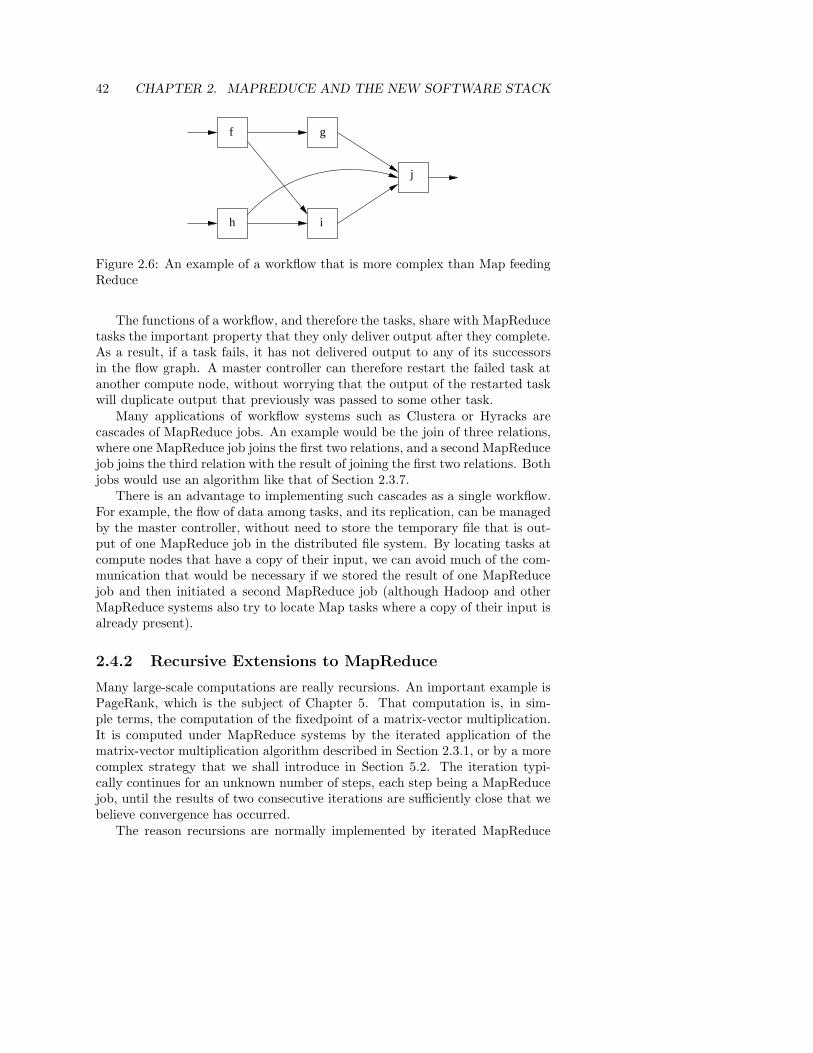
Two experimental systems called Clustera from the University of Wisconsin andHyracks from the University of California at Irvine extend MapReduce from thesimple two-step workflow (the Map function feeds the Reduce function) to anycollection of functions, with an acyclic graph representing workflow among thefunctions. That is, there is an acyclic flow graph whose arcs a → b representthe fact that function a’s output is input to function b. A suggestion of what aworkflow might look like is in Fig. 2.6. There, five functions, f through j, passdata from left to right in specific ways, so the flow of data is acyclic and no taskneeds to provide data out before its input is available. For instance, function htakes its input from a preexisting file of the distributed file system. Each of h’soutput elements is passed to at least one of the functions i and j.
In analogy to Map and Reduce functions, each function of a workflow canbe executed by many tasks, each of which is assigned a portion of the input tothe function. A master controller is responsible for dividing the work amongthe tasks that implement a function, usually by hashing the input elements todecide on the proper task to receive an element. Thus, like Map tasks, each taskimplementing a function f has an output file of data destined for each of thetasks that implement the successor function(s) of f . These files are deliveredby the Master at the appropriate time – after the task has completed its work.
42 CHAPTER 2. MAPREDUCE AND THE NEW SOFTWARE STACK
h
f g
i
j
Figure 2.6: An example of a workflow that is more complex than Map feedingReduce
The functions of a workflow, and therefore the tasks, share with MapReducetasks the important property that they only deliver output after they complete.As a result, if a task fails, it has not delivered output to any of its successorsin the flow graph. A master controller can therefore restart the failed task atanother compute node, without worrying that the output of the restarted taskwill duplicate output that previously was passed to some other task.
Many applications of workflow systems such as Clustera or Hyracks arecascades of MapReduce jobs. An example would be the join of three relations,where one MapReduce job joins the first two relations, and a second MapReducejob joins the third relation with the result of joining the first two relations. Bothjobs would use an algorithm like that of Section 2.3.7.
There is an advantage to implementing such cascades as a single workflow.For example, the flow of data among tasks, and its replication, can be managedby the master controller, without need to store the temporary file that is out-put of one MapReduce job in the distributed file system. By locating tasks atcompute nodes that have a copy of their input, we can avoid much of the com-munication that would be necessary if we stored the result of one MapReducejob and then initiated a second MapReduce job (although Hadoop and otherMapReduce systems also try to locate Map tasks where a copy of their input isalready present).
2.4.2 Recursive Extensions to MapReduce
Many large-scale computations are really recursions. An important example isPageRank, which is the subject of Chapter 5. That computation is, in sim-ple terms, the computation of the fixedpoint of a matrix-vector multiplication.It is computed under MapReduce systems by the iterated application of thematrix-vector multiplication algorithm described in Section 2.3.1, or by a morecomplex strategy that we shall introduce in Section 5.2. The iteration typi-cally continues for an unknown number of steps, each step being a MapReducejob, until the results of two consecutive iterations are sufficiently close that webelieve convergence has occurred.
The reason recursions are normally implemented by iterated MapReduce
2.4. EXTENSIONS TO MAPREDUCE 43
jobs is that a true recursive task does not have the property necessary forindependent restart of failed tasks. It is impossible for a collection of mutuallyrecursive tasks, each of which has an output that is input to at least some ofthe other tasks, to produce output only at the end of the task. If they allfollowed that policy, no task would ever receive any input, and nothing couldbe accomplished. As a result, some mechanism other than simple restart offailed tasks must be implemented in a system that handles recursive workflows(flow graphs that are not acyclic). We shall start by studying an example of arecursion implemented as a workflow, and then discuss approaches to dealingwith task failures.
Example 2.6 : Suppose we have a directed graph whose arcs are representedby the relation E(X, Y ), meaning that there is an arc from node X to node Y .We wish to compute the paths relation P (X, Y ), meaning that there is a pathof length 1 or more from node X to node Y . That is, P is the transitive closureof E. A simple recursive algorithm to do so is:
1. Start with P (X, Y ) = E(X, Y ).
2. While changes to the relation P occur, add to P all tuples in
πX,Y
(
P (X, Z) ⊲⊳ P (Z, Y ))
That is, find pairs of nodes X and Y such that for some node Z there isknown to be a path from X to Z and also a path from Z to Y .
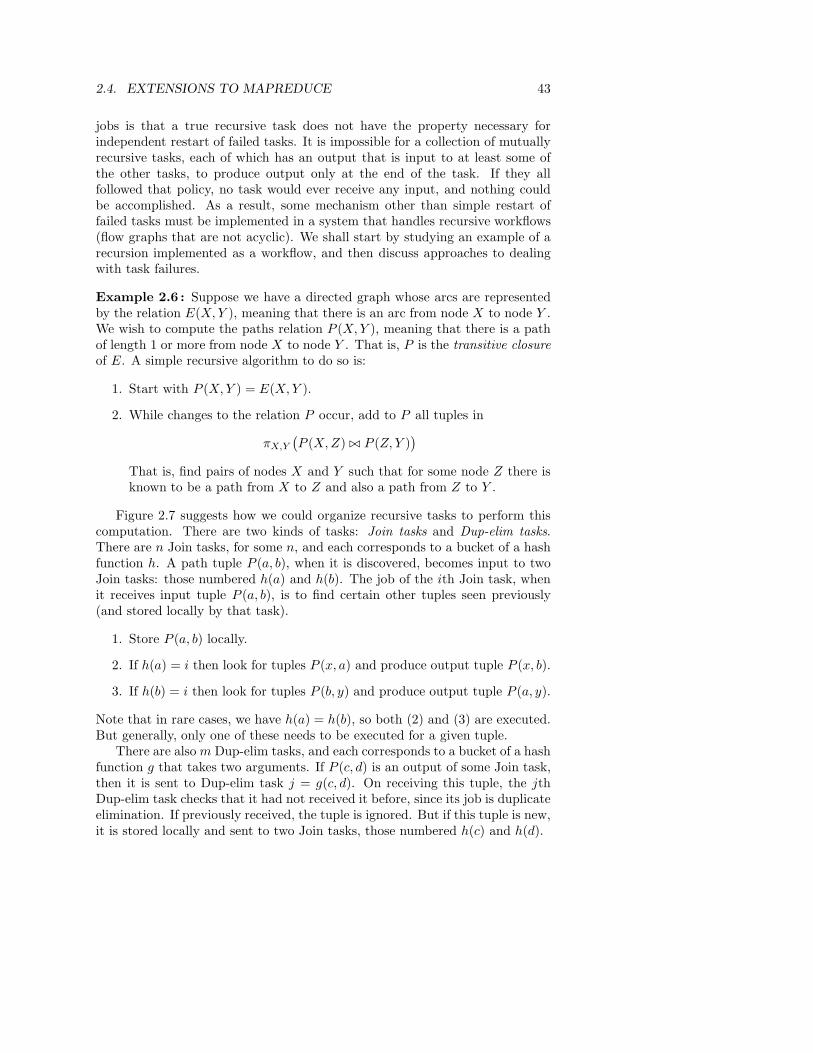
Figure 2.7 suggests how we could organize recursive tasks to perform thiscomputation. There are two kinds of tasks: Join tasks and Dup-elim tasks.There are n Join tasks, for some n, and each corresponds to a bucket of a hashfunction h. A path tuple P (a, b), when it is discovered, becomes input to twoJoin tasks: those numbered h(a) and h(b). The job of the ith Join task, whenit receives input tuple P (a, b), is to find certain other tuples seen previously(and stored locally by that task).
1. Store P (a, b) locally.
2. If h(a) = i then look for tuples P (x, a) and produce output tuple P (x, b).
3. If h(b) = i then look for tuples P (b, y) and produce output tuple P (a, y).
Note that in rare cases, we have h(a) = h(b), so both (2) and (3) are executed.But generally, only one of these needs to be executed for a given tuple.
There are also m Dup-elim tasks, and each corresponds to a bucket of a hashfunction g that takes two arguments. If P (c, d) is an output of some Join task,then it is sent to Dup-elim task j = g(c, d). On receiving this tuple, the jthDup-elim task checks that it had not received it before, since its job is duplicateelimination. If previously received, the tuple is ignored. But if this tuple is new,it is stored locally and sent to two Join tasks, those numbered h(c) and h(d).
44 CHAPTER 2. MAPREDUCE AND THE NEW SOFTWARE STACK
Jointask0
Jointask1
Jointaski
task0
Dup−elim
task1
Dup−elim
taskj
Dup−elim
.
.
.
.
.
.
.
.
.
.
.
.
P(a,b) ifh(a) = i orh(b) = i
P(c,d) ifg(c,d) = j
P(c,d) if neverseen before
To join task h(d)
To join task h(c)
Figure 2.7: Implementation of transitive closure by a collection of recursivetasks
Every Join task has m output files – one for each Dup-elim task – and everyDup-elim task has n output files – one for each Join task. These files may bedistributed according to any of several strategies. Initially, the E(a, b) tuplesrepresenting the arcs of the graph are distributed to the Dup-elim tasks, withE(a, b) being sent as P (a, b) to Dup-elim task g(a, b). The Master can wait untileach Join task has processed its entire input for a round. Then, all output filesare distributed to the Dup-elim tasks, which create their own output. Thatoutput is distributed to the Join tasks and becomes their input for the nextround. Alternatively, each task can wait until it has produced enough outputto justify transmitting its output files to their destination, even if the task hasnot consumed all its input. 2
In Example 2.6 it is not essential to have two kinds of tasks. Rather, Jointasks could eliminate duplicates as they are received, since they must storetheir previously received inputs anyway. However, this arrangement has anadvantage when we must recover from a task failure. If each task stores allthe output files it has ever created, and we place Join tasks on different racksfrom the Dup-elim tasks, then we can deal with any single compute node or
2.4. EXTENSIONS TO MAPREDUCE 45
Pregel and Giraph
Like MapReduce, Pregel was developed originally at Google. Also likeMapReduce, there is an Apache, open-source equivalent, called Giraph.
single rack failure. That is, a Join task needing to be restarted can get all thepreviously generated inputs that it needs from the Dup-elim tasks, and viceversa.
In the particular case of computing transitive closure, it is not necessary toprevent a restarted task from generating outputs that the original task gener-ated previously. In the computation of the transitive closure, the rediscovery ofa path does not influence the eventual answer. However, many computationscannot tolerate a situation where both the original and restarted versions of atask pass the same output to another task. For example, if the final step of thecomputation were an aggregation, say a count of the number of nodes reachedby each node in the graph, then we would get the wrong answer if we counteda path twice. In such a case, the master controller can record what files eachtask generated and passed to other tasks. It can then restart a failed task andignore those files when the restarted version produces them a second time.
2.4.3 Pregel
Another approach to managing failures when implementing recursive algorithmson a computing cluster is represented by the Pregel system. This system viewsits data as a graph. Each node of the graph corresponds roughly to a task(although in practice many nodes of a large graph would be bundled into asingle task, as in the Join tasks of Example 2.6). Each graph node generatesoutput messages that are destined for other nodes of the graph, and each graphnode processes the inputs it receives from other nodes.
Example 2.7 : Suppose our data is a collection of weighted arcs of a graph,and we want to find, for each node of the graph, the length of the shortestpath to each of the other nodes. Initially, each graph node a stores the set ofpairs (b, w) such that there is an arc from a to b of weight w. These facts areinitially sent to all other nodes, as triples (a, b, w).6 When the node a receivesa triple (c, d, w), it looks up its current distance to c; that is, it finds the pair(c, v) stored locally, if there is one. It also finds the pair (d, u) if there is one.If w + v < u, then the pair (d, u) is replaced by (d, w + v), and if there wasno pair (d, u), then the pair (d, w + v) is stored at the node a. Also, the othernodes are sent the message (a, d, w + v) in either of these two cases. 2
6This algorithm uses much too much communication, but it will serve as a simple example
of the Pregel computation model.
46 CHAPTER 2. MAPREDUCE AND THE NEW SOFTWARE STACK
Computations in Pregel are organized into supersteps. In one superstep, allthe messages that were received by any of the nodes at the previous superstep(or initially, if it is the first superstep) are processed, and then all the messagesgenerated by those nodes are sent to their destination.
In case of a compute-node failure, there is no attempt to restart the failedtasks at that compute node. Rather, Pregel checkpoints its entire computationafter some of the supersteps. A checkpoint consists of making a copy of theentire state of each task, so it can be restarted from that point if necessary.If any compute node fails, the entire job is restarted from the most recentcheckpoint.
Although this recovery strategy causes many tasks that have not failed toredo their work, it is satisfactory in many situations. Recall that the reasonMapReduce systems support restart of only the failed tasks is that we wantassurance that the expected time to complete the entire job in the face of fail-ures is not too much greater than the time to run the job with no failures.Any failure-management system will have that property as long as the timeto recover from a failure is much less than the average time between failures.Thus, it is only necessary that Pregel checkpoints its computation after a num-ber of supersteps such that the probability of a failure during that number ofsupersteps is low.
2.4.4 Exercises for Section 2.4
! Exercise 2.4.1 : Suppose a job consists of n tasks, each of which takes time tseconds. Thus, if there are no failures, the sum over all compute nodes of thetime taken to execute tasks at that node is nt. Suppose also that the probabilityof a task failing is p per job per second, and when a task fails, the overhead ofmanagement of the restart is such that it adds 10t seconds to the total executiontime of the job. What is the total expected execution time of the job?
! Exercise 2.4.2 : Suppose a Pregel job has a probability p of a failure duringany superstep. Suppose also that the execution time (summed over all computenodes) of taking a checkpoint is c times the time it takes to execute a superstep.To minimize the expected execution time of the job, how many superstepsshould elapse between checkpoints?
2.5 The Communication Cost Model
In this section we shall introduce a model for measuring the quality of algorithmsimplemented on a computing cluster of the type so far discussed in this chapter.We assume the computation is described by an acyclic workflow, as discussedin Section 2.4.1. For many applications, the bottleneck is moving data amongtasks, such as transporting the outputs of Map tasks to their proper Reducetasks. As an example, we explore the computation of multiway joins as single
2.5. THE COMMUNICATION COST MODEL 47
MapReduce jobs, and we see that in some situations, this approach is moreefficient than the straightforward cascade of 2-way joins.
2.5.1 Communication-Cost for Task Networks
Imagine that an algorithm is implemented by an acyclic network of tasks. Thesetasks could be Map tasks feeding Reduce tasks, as in a standard MapReducealgorithm, or they could be several MapReduce jobs cascaded, or a more generalworkflow structure, such as a collection of tasks each of which implements theworkflow of Fig. 2.6.7 The communication cost of a task is the size of the inputto the task. This size can be measured in bytes. However, since we shall beusing relational database operations as examples, we shall often use the numberof tuples as a measure of size.
The communication cost of an algorithm is the sum of the communicationcost of all the tasks implementing that algorithm. We shall focus on the commu-nication cost as the way to measure the efficiency of an algorithm. In particular,we do not consider the amount of time it takes each task to execute when es-timating the running time of an algorithm. While there are exceptions, whereexecution time of tasks dominates, these exceptions are rare in practice. Wecan explain and justify the importance of communication cost as follows.
• The algorithm executed by each task tends to be very simple, often linearin the size of its input.
• The typical interconnect speed for a computing cluster is one gigabit persecond. That may seem like a lot, but it is slow compared with the speedat which a processor executes instructions. Moreover, in many clusterarchitectures, there is competition for the interconnect when several com-pute nodes need to communicate at the same time. As a result, thecompute node can do a lot of work on a received input element in thetime it takes to deliver that element.
• Even if a task executes at a compute node that has a copy of the chunk(s)on which the task operates, that chunk normally will be stored on disk,and the time taken to move the data into main memory may exceed thetime needed to operate on the data once it is available in memory.
Assuming that communication cost is the dominant cost, we might still askwhy we count only input size, and not output size. The answer to this questioninvolves two points:
1. If the output of one task τ is input to another task, then the size of τ ’soutput will be accounted for when measuring the input size for the receiv-ing task. Thus, there is no reason to count the size of any output exceptfor those tasks whose output forms the result of the entire algorithm.
7Recall that this figure represented functions, not tasks. As a network of tasks, there
would be, for example, many tasks implementing function f , each of which feeds data to each
of the tasks for function g and each of the tasks for function i.
48 CHAPTER 2. MAPREDUCE AND THE NEW SOFTWARE STACK
2. But in practice, the algorithm output is rarely large compared with theinput or the intermediate data produced by the algorithm. The reasonis that massive outputs cannot be used unless they are summarized oraggregated in some way. For example, although we talked in Example 2.6of computing the entire transitive closure of a graph, in practice we wouldwant something much simpler, such as the count of the number of nodesreachable from each node, or the set of nodes reachable from a singlenode.
Example 2.8 : Let us evaluate the communication cost for the join algorithmfrom Section 2.3.7. Suppose we are joining R(A, B) ⊲⊳ S(B, C), and the sizesof relations R and S are r and s, respectively. Each chunk of the files holdingR and S is fed to one Map task, so the sum of the communication costs for allthe Map tasks is r + s. Note that in a typical execution, the Map tasks willeach be executed at a compute node holding a copy of the chunk to which itapplies. Thus, no internode communication is needed for the Map tasks, butthey still must read their data from disk. Since all the Map tasks do is make asimple transformation of each input tuple into a key-value pair, we expect thatthe computation cost will be small compared with the communication cost,regardless of whether the input is local to the task or must be transported toits compute node.
The sum of the outputs of the Map tasks is roughly as large as their in-puts. Each output key-value pair is sent to exactly one Reduce task, and it isunlikely that this Reduce task will execute at the same compute node. There-fore, communication from Map tasks to Reduce tasks is likely to be across theinterconnect of the cluster, rather than memory-to-disk. This communicationis O(r + s), so the communication cost of the join algorithm is O(r + s).
The Reduce tasks execute the reducer (application of the Reduce functionto a key and its associated value list) for one or more values of attribute B.Each reducer takes the inputs it receives and divides them between tuples thatcame from R and those that came from S. Each tuple from R pairs with eachtuple from S to produce one output. The output size for the join can be eitherlarger or smaller than r + s, depending on how likely it is that a given R-tuplejoins with a given S-tuple. For example, if there are many different B-values,we would expect the output to be small, while if there are few B-values, a largeoutput is likely.
If the output is large, then the computation cost of generating all the outputsfrom a reducer could be much larger than O(r+s). However, we shall rely on oursupposition that if the output of the join is large, then there is probably someaggregation being done to reduce the size of the output. It will be necessary tocommunicate the result of the join to another collection of tasks that performthis aggregation, and thus the communication cost will be at least proportionalto the computation needed to produce the output of the join. 2
2.5. THE COMMUNICATION COST MODEL 49
2.5.2 Wall-Clock Time
While communication cost often influences our choice of algorithm to use ina cluster-computing environment, we must also be aware of the importance ofwall-clock time, the time it takes a parallel algorithm to finish. Using carelessreasoning, one could minimize total communication cost by assigning all thework to one task, and thereby minimize total communication. However, thewall-clock time of such an algorithm would be quite high. The algorithms wesuggest, or have suggested so far, have the property that the work is dividedfairly among the tasks. Therefore, the wall-clock time would be approximatelyas small as it could be, given the number of compute nodes available.
2.5.3 Multiway Joins
To see how analyzing the communication cost can help us choose an algorithmin the cluster-computing environment, we shall examine carefully the case of amultiway join. There is a general theory in which we:
1. Select certain attributes of the relations involved in the natural join ofthree or more relations to have their values hashed, each to some numberof buckets.
2. Select the number of buckets for each of these attributes, subject to theconstraint that the product of the numbers of buckets for each attributeis k, the number of reducers that will be used.
3. Identify each of the k reducers with a vector of bucket numbers. Thesevectors have one component for each of the attributes selected at step (1).
4. Send tuples of each relation to all those reducers where it might find tuplesto join with. That is, the given tuple t will have values for some of theattributes selected at step (1), so we can apply the hash function(s) tothose values to determine certain components of the vector that identifiesthe reducers. Other components of the vector are unknown, so t mustbe sent to reducers for all vectors having any value in these unknowncomponents.
Some examples of this general technique appear in the exercises.Here, we shall look only at the join R(A, B) ⊲⊳ S(B, C) ⊲⊳ T (C, D) as
an example. Suppose that the relations R, S, and T have sizes r, s, and t,respectively, and for simplicity, suppose p is the probability that
1. An R-tuple and and S-tuple agree on B, and also the probability that
2. An S-tuple and a T -tuple agree on C.
If we join R and S first, using the MapReduce algorithm of Section 2.3.7,then the communication cost is O(r + s), and the size of the intermediate join
50 CHAPTER 2. MAPREDUCE AND THE NEW SOFTWARE STACK
R ⊲⊳ S is prs. When we join this result with T , the communication of thissecond MapReduce job is O(t + prs). Thus, the entire communication cost ofthe algorithm consisting of two 2-way joins is O(r + s + t + prs). If we insteadjoin S and T first, and then join R with the result, we get another algorithmwhose communication cost is O(r + s + t + pst).
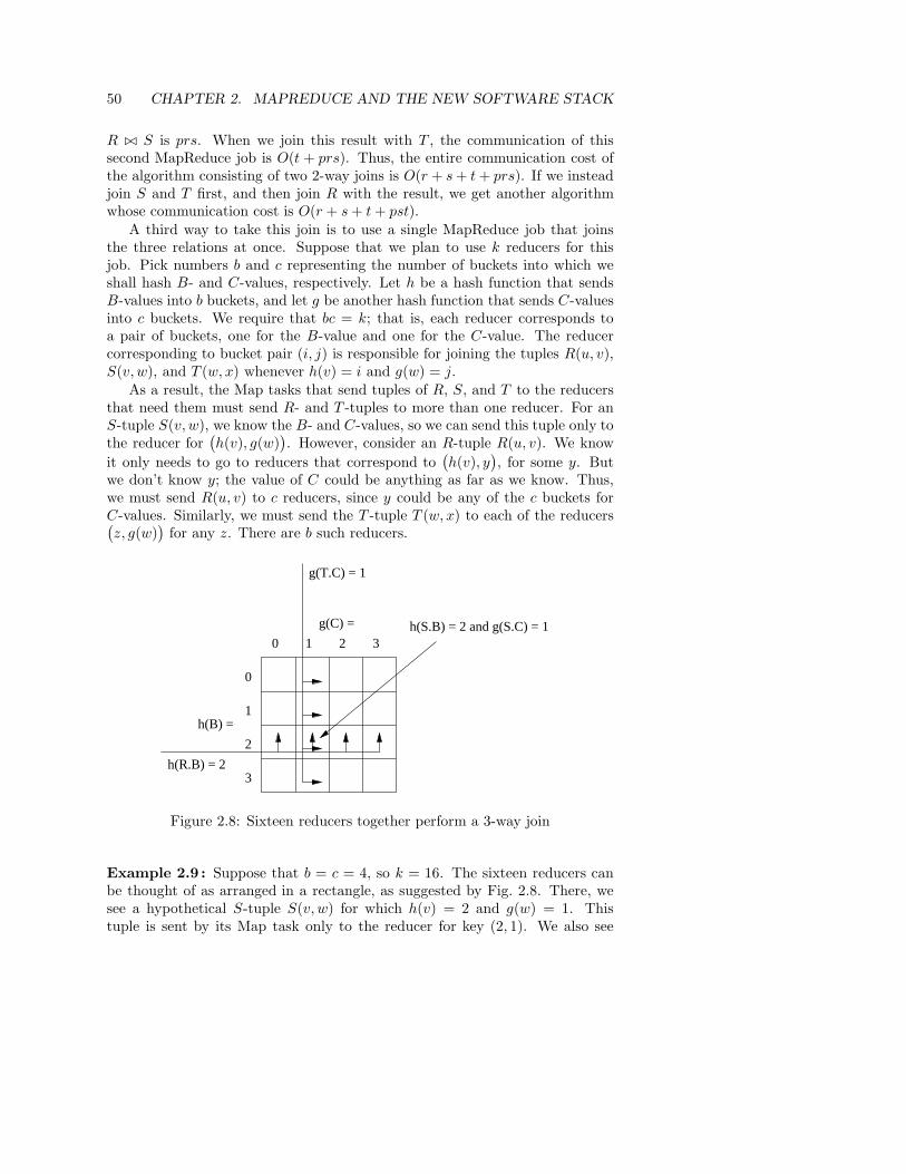
A third way to take this join is to use a single MapReduce job that joinsthe three relations at once. Suppose that we plan to use k reducers for thisjob. Pick numbers b and c representing the number of buckets into which weshall hash B- and C-values, respectively. Let h be a hash function that sendsB-values into b buckets, and let g be another hash function that sends C-valuesinto c buckets. We require that bc = k; that is, each reducer corresponds toa pair of buckets, one for the B-value and one for the C-value. The reducercorresponding to bucket pair (i, j) is responsible for joining the tuples R(u, v),S(v, w), and T (w, x) whenever h(v) = i and g(w) = j.
As a result, the Map tasks that send tuples of R, S, and T to the reducersthat need them must send R- and T -tuples to more than one reducer. For anS-tuple S(v, w), we know the B- and C-values, so we can send this tuple only tothe reducer for
(
h(v), g(w))
. However, consider an R-tuple R(u, v). We know
it only needs to go to reducers that correspond to(
h(v), y)
, for some y. Butwe don’t know y; the value of C could be anything as far as we know. Thus,we must send R(u, v) to c reducers, since y could be any of the c buckets forC-values. Similarly, we must send the T -tuple T (w, x) to each of the reducers(
z, g(w))
for any z. There are b such reducers.
0 1 2 3
2
1
0
g(T.C) = 1
g(C) = h(S.B) = 2 and g(S.C) = 1
h(B) =
h(R.B) = 23
Figure 2.8: Sixteen reducers together perform a 3-way join
Example 2.9 : Suppose that b = c = 4, so k = 16. The sixteen reducers canbe thought of as arranged in a rectangle, as suggested by Fig. 2.8. There, wesee a hypothetical S-tuple S(v, w) for which h(v) = 2 and g(w) = 1. Thistuple is sent by its Map task only to the reducer for key (2, 1). We also see
2.5. THE COMMUNICATION COST MODEL 51
Computation Cost of the 3-Way Join
Each of the reducers must join of parts of the three relations, and it isreasonable to ask whether this join can be taken in time that is linearin the size of the input to that Reduce task. While more complex joinsmight not be computable in linear time, the join of our running examplecan be executed at each Reduce process efficiently. First, create an indexon R.B, to organize the R-tuples received. Likewise, create an index onT.C for the T -tuples. Then, consider each received S-tuple, S(v, w). Usethe index on R.B to find all R-tuples with R.B = v and use the index onT.C to find all T -tuples with T.C = w.
an R-tuple R(u, v). Since h(v) = 2, this tuple is sent to all reducers (2, y), fory = 1, 2, 3, 4. Finally, we see a T -tuple T (w, x). Since g(w) = 1, this tuple issent to all reducers (z, 1) for z = 1, 2, 3, 4. Notice that these three tuples join,and they meet at exactly one reducer, the reducer for key (2, 1). 2
Now, suppose that the sizes of R, S, and T are different; recall we use r,s, and t, respectively, for those sizes. If we hash B-values to b buckets andC-values to c buckets, where bc = k, then the total communication cost formoving the tuples to the proper reducers is the sum of:
1. s to move each tuple S(v, w) once to the reducer(
h(v), g(w))
.
2. cr to move each tuple R(u, v) to the c reducers(
h(v), y)
for each of the cpossible values of y.
3. bt to move each tuple T (w, x) to the b reducers(
z, g(w))
for each of theb possible values of z.
There is also a cost r + s + t to make each tuple of each relation be input toone of the Map tasks. This cost is fixed, independent of b, c, and k.
We must select b and c, subject to the constraint bc = k, to minimizes + cr + bt. We shall use the technique of Lagrangean multipliers to find theplace where the function s + cr + bt− λ(bc− k) has its derivatives with respectto b and c equal to 0. That is, we must solve the equations r − λb = 0 andt − λc = 0. Since r = λb and t = λc, we may multiply corresponding sides ofthese equations to get rt = λ2bc. Since bc = k, we get rt = λ2k, or λ =
√
rt/k.
Thus, the minimum communication cost is obtained when c = t/λ =√
kt/r,
and b = r/λ =√
kr/t.
If we substitute these values into the formula s + cr + bt, we get s + 2√
krt.That is the communication cost for the Reduce tasks, to which we must addthe cost s + r + t for the communication cost of the Map tasks. The total
52 CHAPTER 2. MAPREDUCE AND THE NEW SOFTWARE STACK
communication cost is thus r + 2s + t + 2√
krt. In most circumstances, we canneglect r + t, because it will be less than 2
√krt, usually by a factor of O(
√k).
Example 2.10 : Let us see under what circumstances the 3-way join has lowercommunication cost than the cascade of two 2-way joins. To make matterssimple, let us assume that R, S, and T are all the same relation R, whichrepresents the “friends” relation in a social network like Facebook. There areroughly a billion subscribers on Facebook, with an average of 300 friends each, sorelation R has r = 3 × 10¹¹ tuples. Suppose we want to compute R ⊲⊳ R ⊲⊳ R,perhaps as part of a calculation to find the number of friends of friends offriends each subscriber has, or perhaps just the person with the largest numberof friends of friends of friends.8 The cost of the 3-way join of R with itself is4r + 2r
√k; 3r represents the cost of the Map tasks, and r + 2
√kr2 is the cost
of the Reduce tasks. Since we assume r = 3× 10¹¹, this cost is 1, 2× 10¹² +6×10¹¹
√k.
Now consider the communication cost of joining R with itself, and thenjoining the result with R again. The Map and Reduce tasks for the first join eachhave a cost of 2r, so the first join only has communication cost 4r = 1.2× 10¹².But the size of R ⊲⊳ R is large. We cannot say exactly how large, since friendstend to fall into cliques, and therefore a person with 300 friends will have manyfewer than the maximum possible number of friends of friends, which is 90,000.Let us estimate conservatively that the size of R ⊲⊳ R is not 300r, but only30r, or 9 × 10¹². The communication cost for the second join of (R ⊲⊳ R) ⊲⊳ Ris thus 1.8 × 10¹³ + 6 × 10¹¹. The total cost of the two joins is therefore1.2 × 1012 + 1.8 × 10¹³ + 6 × 1011 = 1.98 × 10¹³.
We must ask whether the cost of the 3-way join, which is
1.2 × 10¹² + 6 × 10¹¹√
k
is less than 1.98 × 10¹³. That is so, provided 6 × 10¹¹√
k < 1.86 × 10¹³, or√k < 31. That is, the 3-way join will be preferable provided we use no more
than 312 = 961 reducers. 2
2.5.4 Exercises for Section 2.5
Exercise 2.5.1 : What is the communication cost of each of the followingalgorithms, as a function of the size of the relations, matrices, or vectors towhich they are applied?
(a) The matrix-vector multiplication algorithm of Section 2.3.2.
(b) The union algorithm of Section 2.3.6.
(c) The aggregation algorithm of Section 2.3.8.
8This person, or more generally, people with large extended circles of friends, are good
people to use to start a marketing campaign by giving them free samples.
2.5. THE COMMUNICATION COST MODEL 53
Star Joins
A common structure for data mining of commercial data is the star join.For example, a chain store like Walmart keeps a fact table whose tu-ples each represent a single sale. This relation looks like F (A1, A2, . . .),where each attribute Ai is a key representing one of the important com-ponents of the sale, such as the purchaser, the item purchased, the storebranch, or the date. For each key attribute there is a dimension tablegiving information about the participant. For instance, the dimension ta-ble D(A1, B11, B12, . . .) might represent purchasers. A1 is the purchaserID, the key for this relation. The B1i’s might give the purchaser’s name,address, phone, and so on. Typically, the fact table is much larger thanthe dimension tables. For instance, there might be a fact table of a billiontuples and ten dimension tables of a million tuples each.
Analysts mine this data by asking analytic queries that typically jointhe fact table with several of the dimension tables (a “star join”) and thenaggregate the result into a useful form. For instance, an analyst might ask“give me a table of sales of pants, broken down by region and color, foreach month of 2012.” Under the communication-cost model of this section,joining the fact table and dimension tables by a multiway join is almostcertain to be more efficient than joining the relations in pairs. In fact, itmay make sense to store the fact table over however many compute nodesare available, and replicate the dimension tables permanently in exactlythe same way as we would replicate them should we take the join of thefact table and all the dimension tables. In this special case, only thekey attributes (the A’s above) are hashed to buckets, and the number ofbuckets for each key attribute is proportional to the size of its dimensiontable.
(d) The matrix-multiplication algorithm of Section 2.3.10.
! Exercise 2.5.2 : Suppose relations R, S, and T have sizes r, s, and t, respec-tively, and we want to take the 3-way join R(A, B) ⊲⊳ S(B, C) ⊲⊳ T (A, C),using k reducers. We shall hash values of attributes A, B, and C to a, b, and cbuckets, respectively, where abc = k. Each reducer is associated with a vectorof buckets, one for each of the three hash functions. Find, as a function of r, s,t, and k, the values of a, b, and c that minimize the communication cost of thealgorithm.
! Exercise 2.5.3 : Suppose we take a star join of a fact table F (A1, A2, . . . , Am)with dimension tables Di(Ai, Bi) for i = 1, 2, . . . , m. Let there be k reducers,each associated with a vector of buckets, one for each of the key attributesA1, A2, . . . , Am. Suppose the number of buckets into which we hash Ai is ai.
54 CHAPTER 2. MAPREDUCE AND THE NEW SOFTWARE STACK
Naturally, a1a2 · · · am = k. Finally, suppose each dimension table Di has sizedi, and the size of the fact table is much larger than any of these sizes. Findthe values of the ai’s that minimize the cost of taking the star join as oneMapReduce operation.
2.6 Complexity Theory for MapReduce
Now, we shall explore the design of MapReduce algorithms in more detail. Sec-tion 2.5 introduced the idea that communication between the Map and Reducetasks often accounts for the largest fraction of the time spent by these tasks.Here, we shall look at how the communication cost relates to other desideratafor MapReduce algorithms, in particular our desire to shrink the wall-clock timeand to execute each reducer in main memory. Recall that a “reducer” is theexecution of the Reduce function on a single key and its associated value list.The point of the exploration in this section is that for many problems there is aspectrum of MapReduce algorithms requiring different amounts of communica-tion. Moreover, the less communication an algorithm uses, the worse it may bein other respects, including wall-clock time and the amount of main memory itrequires.
2.6.1 Reducer Size and Replication Rate
Let us now introduce the two parameters that characterize families of MapRe-duce algorithms. The first is the reducer size, which we denote by q. Thisparameter is the upper bound on the number of values that are allowed to ap-pear in the list associated with a single key. Reducer size can be selected withat least two goals in mind.
1. By making the reducer size small, we can force there to be many reducers,i.e., many different keys according to which the problem input is dividedby the Map tasks. If we also create many Reduce tasks – even one foreach reducer – then there will be a high degree of parallelism, and we canlook forward to a low wall-clock time.
2. We can choose a reducer size sufficiently small that we are certain thecomputation associated with a single reducer can be executed entirely inthe main memory of the compute node where its Reduce task is located.Regardless of the computation done by the reducers, the running timewill be greatly reduced if we can avoid having to move data repeatedlybetween main memory and disk.
The second parameter is the replication rate, denoted r. We define r tobe the number of key-value pairs produced by all the Map tasks on all theinputs, divided by the number of inputs. That is, the replication rate is theaverage communication from Map tasks to Reduce tasks (measured by countingkey-value pairs) per input.
2.6. COMPLEXITY THEORY FOR MAPREDUCE 55
Example 2.11 : Let us consider the one-pass matrix-multiplication algorithmof Section 2.3.10. Suppose that all the matrices involved are n × n matrices.Then the replication rate r is equal to n. That fact is easy to see, since foreach element mij , there are n key-value pairs produced; these have all keys ofthe form (i, k), for 1 ≤ k ≤ n. Likewise, for each element of the other matrix,say njk, we produce n key-value pairs, each having one of the keys (i, k), for1 ≤ i ≤ n. In this case, not only is n the average number of key-value pairsproduced for an input element, but each input produces exactly this number ofpairs.
We also see that q, the required reducer size, is 2n. That is, for each key(i, k), there are n key-value pairs representing elements mij of the first matrixand another n key-value pairs derived from the elements njk of the secondmatrix. While this pair of values represents only one particular algorithm forone-pass matrix multiplication, we shall see that it is part of a spectrum ofalgorithms, and in fact represents an extreme point, where q is as small as canbe, and r is at its maximum. More generally, there is a tradeoff between r andq, that can be expressed as qr ≥ 2n2. 2
2.6.2 An Example: Similarity Joins
To see the tradeoff between r and q in a realistic situation, we shall examine aproblem known as similarity join. In this problem, we are given a large set ofelements X and a similarity measure s(x, y) that tells how similar two elementsx and y of set X are. In Chapter 3 we shall learn about the most importantnotions of similarity and also learn some tricks that let us find similar pairsquickly. But here, we shall consider only the raw form of the problem, wherewe have to look at each pair of elements of X and determine their similarity byapplying the function s. We assume that s is symmetric, so s(x, y) = s(y, x),but we assume nothing else about s. The output of the algorithm is those pairswhose similarity exceeds a given threshold t.
For example, let us suppose we have a collection of one million images, eachof size one megabyte. Thus, the dataset has size one terabyte. We shall nottry to describe the similarity function s, but it might, say, involve giving highervalues when images have roughly the same distribution of colors or when imageshave corresponding regions with the same distribution of colors. The goal wouldbe to discover pairs of images that show the same type of object or scene. Thisproblem is extremely hard, but classifying by color distribution is generally ofsome help toward that goal.
Let us look at how we might do the computation using MapReduce to exploitthe natural parallelism found in this problem. The input is key-value pairs(i, Pi), where i is an ID for the picture and Pi is the picture itself. We wantto compare each pair of pictures, so let us use one key for each set of two ID’s{i, j}. There are approximately 5 × 10¹¹ pairs of two ID’s. We want eachkey {i, j} to be associated with the two values Pi and Pj , so the input to thecorresponding reducer will be ({i, j}, [Pi, Pj ]). Then, the Reduce function can
56 CHAPTER 2. MAPREDUCE AND THE NEW SOFTWARE STACK
simply apply the similarity function s to the two pictures on its value list, thatis, compute s(Pi, Pj), and decide whether the similarity of the two pictures isabove threshold. The pair would be output if so.
Alas, this algorithm will fail completely. The reducer size is small, since nolist has more than two values, or a total of 2MB of input. Although we don’tknow exactly how the similarity function s operates, we can reasonably expectthat it will not require more than the available main memory. However, thereplication rate is 999,999, since for each picture we generate that number ofkey-value pairs, one for each of the other pictures in the dataset. The totalnumber of bytes communicated from Map tasks to Reduce tasks is 1,000,000(for the pictures) times 999,999 (for the replication), times 1,000,000 (for thesize of each picture). That’s 1018 bytes, or one exabyte. To communicate thisamount of data over gigabit Ethernet would take 1010 seconds, or about 300years.9
Fortunately, this algorithm is only the extreme point in a spectrum of possi-ble algorithms. We can characterize these algorithms by grouping pictures intog groups, each of 106/g pictures.
The Map Function: Take an input element (i, Pi) and generate g − 1 key-value pairs. For each, the key is one of the sets {u, v}, where u is the group towhich picture i belongs, and v is one of the other groups. The associated valueis the pair (i, Pi).
The Reduce Function: Consider the key {u, v}. The associated value listwill have the 2 × 10⁶/g elements (j, Pj), where j belongs to either group u orgroup v. The Reduce function takes each (i, Pi) and (j, Pj) on this list, wherei and j belong to different groups, and applies the similarity function s(Pi, Pj).In addition, we need to compare the pictures that belong to the same group,but we don’t want to do the same comparison at each of the g − 1 reducerswhose key contains a given group number. There are many ways to handle thisproblem, but one way is as follows. Compare the members of group u at thereducer {u, u + 1}, where the “+1” is taken in the end-around sense. That is,if u = g (i.e., u is the last group), then u + 1 is group 1. Otherwise, u + 1 is thegroup whose number is one greater than u.
We can compute the replication rate and reducer size as a function of thenumber of groups g. Each input element is turned into g − 1 key-value pairs.That is, the replication rate is g − 1, or approximately r = g, since we supposethat the number of groups is still fairly large. The reducer size is 2×10⁶/g, sincethat is the number of values on the list for each reducer. Each value is about amegabyte, so the number of bytes needed to store the input is 2 × 10¹²/g.
Example 2.12 : If g is 1000, then the input consumes about 2GB. That’senough to hold everything in a typical main memory. Moreover, the total
9In a typical cluster, there are many switches connecting subsets of the compute nodes, so
all the data does not need to go across a single gigabit switch. However, the total available
communication is still small enough that it is not feasible to implement this algorithm for the
scale of data we have hypothesized.
2.6. COMPLEXITY THEORY FOR MAPREDUCE 57
number of bytes communicated is now 106 × 999 × 106, or about 1015 bytes.While that is still a huge amount of data to communicate, it is 1000 timesless than that of the obvious algorithm. Moreover, there are still about half amillion reducers. Since we are unlikely to have available that many computenodes, we can divide all the reducers into a smaller number of Reduce tasksand still keep all the compute nodes busy; i.e., we can get as much parallelismas our computing cluster offers us. 2
The computation cost for algorithms in this family is independent of thenumber of groups g, as long as the input to each reducer fits in main memory.The reason is that the bulk of the computation is the application of function sto the pairs of pictures. No matter what value g has, s is applied to each paironce and only once. Thus, although the work of algorithms in the family maybe divided among reducers in widely different ways, all members of the familydo the same computation.
2.6.3 A Graph Model for MapReduce Problems
In this section, we begin the study of a technique that will enable us to provelower bounds on the replication rate, as a function of reducer size for a numberof problems. Our first step is to introduce a graph model of problems. For eachproblem solvable by a MapReduce algorithm there is:
1. A set of inputs.
2. A set of outputs.
3. A many-many relationship between the inputs and outputs, which de-scribes which inputs are necessary to produce which outputs.
Example 2.13 : Figure 2.9 shows the graph for the similarity-join problemdiscussed in Section 2.6.2, if there were four pictures rather than a million. Theinputs are the pictures, and the outputs are the six possible pairs of pictures.Each output is related to the two inputs that are members of its pair. 2
Example 2.14 : Matrix multiplication presents a more complex graph. If wemultiply n × n matrices M and N to get matrix P , then there are 2n2 inputs,mij and njk, and there are n2 outputs pik. Each output pik is related to 2ninputs: mi1, mi2, . . . , min and n1k, n2k, . . . , nnk. Moreover, each input is relatedto n outputs. For example, mij is related to pi1, pi2, . . . , pin. Figure 2.10 showsthe input-output relationship for matrix multiplication for the simple case of2 × 2 matrices, specifically
[
a bc d
] [
e fg h
]
=
[
i jk l
]
2
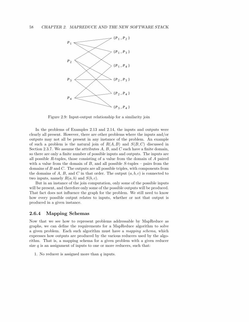
58 CHAPTER 2. MAPREDUCE AND THE NEW SOFTWARE STACK
P 1
P 2
P 3
P 4
P 1
P 1
P 1
P 2
P 3
P 4
P 2
P 2
P 3
P 4
P 3 P 4
{ , }
{ , }
{ , }
{ , }
{ , }
{ , }
Figure 2.9: Input-output relationship for a similarity join
In the problems of Examples 2.13 and 2.14, the inputs and outputs wereclearly all present. However, there are other problems where the inputs and/oroutputs may not all be present in any instance of the problem. An exampleof such a problem is the natural join of R(A, B) and S(B, C) discussed inSection 2.3.7. We assume the attributes A, B, and C each have a finite domain,so there are only a finite number of possible inputs and outputs. The inputs areall possible R-tuples, those consisting of a value from the domain of A pairedwith a value from the domain of B, and all possible S-tuples – pairs from thedomains of B and C. The outputs are all possible triples, with components fromthe domains of A, B, and C in that order. The output (a, b, c) is connected totwo inputs, namely R(a, b) and S(b, c).
But in an instance of the join computation, only some of the possible inputswill be present, and therefore only some of the possible outputs will be produced.That fact does not influence the graph for the problem. We still need to knowhow every possible output relates to inputs, whether or not that output isproduced in a given instance.
2.6.4 Mapping Schemas
Now that we see how to represent problems addressable by MapReduce asgraphs, we can define the requirements for a MapReduce algorithm to solvea given problem. Each such algorithm must have a mapping schema, whichexpresses how outputs are produced by the various reducers used by the algo-rithm. That is, a mapping schema for a given problem with a given reducersize q is an assignment of inputs to one or more reducers, such that:
1. No reducer is assigned more than q inputs.
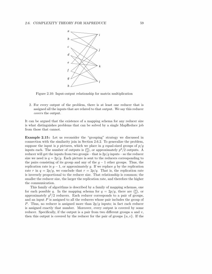
2.6. COMPLEXITY THEORY FOR MAPREDUCE 59
a
b
c
d
e
f
g
h
i
j
k
l
Figure 2.10: Input-output relationship for matrix multiplication
2. For every output of the problem, there is at least one reducer that isassigned all the inputs that are related to that output. We say this reducercovers the output.
It can be argued that the existence of a mapping schema for any reducer sizeis what distinguishes problems that can be solved by a single MapReduce jobfrom those that cannot.
Example 2.15 : Let us reconsider the “grouping” strategy we discussed inconnection with the similarity join in Section 2.6.2. To generalize the problem,suppose the input is p pictures, which we place in g equal-sized groups of p/ginputs each. The number of outputs is
(
p2
)
, or approximately p2/2 outputs. Areducer will get the inputs from two groups – that is 2p/g inputs – so the reducersize we need is q = 2p/g. Each picture is sent to the reducers corresponding tothe pairs consisting of its group and any of the g − 1 other groups. Thus, thereplication rate is g − 1, or approximately g. If we replace g by the replicationrate r in q = 2p/g, we conclude that r = 2p/q. That is, the replication rateis inversely proportional to the reducer size. That relationship is common; thesmaller the reducer size, the larger the replication rate, and therefore the higherthe communication.
This family of algorithms is described by a family of mapping schemas, onefor each possible q. In the mapping schema for q = 2p/g, there are
(
g2
)
, orapproximately g2/2 reducers. Each reducer corresponds to a pair of groups,and an input P is assigned to all the reducers whose pair includes the group ofP . Thus, no reducer is assigned more than 2p/g inputs; in fact each reduceris assigned exactly that number. Moreover, every output is covered by somereducer. Specifically, if the output is a pair from two different groups u and v,then this output is covered by the reducer for the pair of groups {u, v}. If the
60 CHAPTER 2. MAPREDUCE AND THE NEW SOFTWARE STACK
output corresponds to inputs from only one group u, then the output is coveredby several reducers – those corresponding to the set of groups {u, v} for anyv 6= u. Note that the algorithm we described has only one of these reducerscomputing the output, but any of them could compute it. 2
The fact that an output depends on a certain input means that when thatinput is processed at the Map task, there will be at least one key-value pairgenerated to be used when computing that output. The value might not beexactly the input (as was the case in Example 2.15), but it is derived fromthat input. What is important is that for every related input and output thereis a unique key-value pair that must be communicated. Note that there istechnically never a need for more than one key-value pair for a given input andoutput, because the input could be transmitted to the reducer as itself, andwhatever transformations on the input were applied by the Map function couldinstead be applied by the Reduce function at the reducer for that output.
2.6.5 When Not All Inputs Are Present
Example 2.15 describes a problem where we know every possible input is pre-sent, because we can define the input set to be those pictures that actuallyexist in the dataset. However, as discussed at the end of Section 2.6.3, thereare problems like computing the join, where the graph of inputs and outputsdescribes inputs that might exist, and outputs that are only made when at leastone of the inputs exists in the dataset. In fact, for the join, both inputs relatedto an output must exist if we are to make that output.
An algorithm for a problem where outputs can be missing still needs amapping schema. The justification is that all inputs, or any subset of them,might be present, so an algorithm without a mapping schema would not beable to produce every possible output if all the inputs related to that outputhappened to be present, and yet no reducer covered that output.
The only way the absence of some inputs makes a difference is that wemay wish to rethink the desired value of the reducer size q when we select analgorithm from the family of possible algorithms. Especially, if the value of qwe select is that number such that we can be sure the input will just fit in mainmemory, then we may wish to increase q to take into account that some fractionof the inputs are not really there.
Example 2.16 : Suppose that we know we can execute the Reduce functionin main memory on a key and its associated list of q values. However, we alsoknow that only 5% of the possible inputs are really present in the data set.Then a mapping schema for reducer size q will really send about q/20 of theinputs that exist to each reducer. Put another way, we could use the algorithmfor reducer size 20q and expect that an average of q inputs will actually appearon the list for each reducer. We can thus choose 20q as the reducer size, or sincethere will be some randomness in the number of inputs actually appearing at
2.6. COMPLEXITY THEORY FOR MAPREDUCE 61
each reducer, we might wish to pick a slightly smaller value of reducer size, suchas 18q. 2
2.6.6 Lower Bounds on Replication Rate
The family of similarity-join algorithms described in Example 2.15 lets us tradeoff communication against the reducer size, and through reducer size to tradecommunication against parallelism or against the ability to execute the Reducefunction in main memory. How do we know we are getting the best possibletradeoff? We can only know we have the minimum possible communication ifwe can prove a matching lower bound. Using existence of a mapping schema asthe starting point, we can often prove such a lower bound. Here is an outlineof the technique.
1. Prove an upper bound on how many outputs a reducer with q inputs cancover. Call this bound g(q). This step can be difficult, but for exampleslike similarity join, it is actually quite simple.
2. Determine the total number of outputs produced by the problem.
3. Suppose that there are k reducers, and the ith reducer has qi < q inputs.Observe that
∑ki=1 g(qi) must be no less than the number of outputs
computed in step (2).
4. Manipulate the inequality from (3) to get a lower bound on∑k
i=1 qi.Often, the trick used at this step is to replace some factors of qi by theirupper bound q, but leave a single factor of qi in the term for i.
5. Since∑k
i=1 qi is the total communication from Map tasks to Reduce tasks,divide the lower bound from (4) on this quantity by the number of inputs.The result is a lower bound on the replication rate.
Example 2.17 : This sequence of steps may seem mysterious, but let us con-sider the similarity join as an example that we hope will make things clear.Recall that in Example 2.15 we gave an upper bound on the replication rater of r ≤ 2p/q, where p was the number of inputs and q was the reducer size.We shall show a lower bound on r that is half that amount, which implies that,although improvements to the algorithm might be possible, any reduction incommunication for a given reducer size will be by a factor of 2 at most.
For step (1), observe that if a reducer gets q inputs, it cannot cover morethan
(
q2
)
, or approximately q2/2 outputs. For step (2), we know there are a
total of(
p2
)
, or approximately p2/2 outputs that each must be covered. Theinequality constructed at step (3) is thus
k∑
i=1
q2i /2 ≥ p2/2
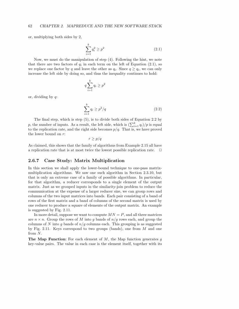
62 CHAPTER 2. MAPREDUCE AND THE NEW SOFTWARE STACK
or, multiplying both sides by 2,
k∑
i=1
q2i ≥ p2 (2.1)
Now, we must do the manipulation of step (4). Following the hint, we notethat there are two factors of qi in each term on the left of Equation (2.1), sowe replace one factor by q and leave the other as qi. Since q ≥ qi, we can onlyincrease the left side by doing so, and thus the inequality continues to hold:
q
k∑
i=1
qi ≥ p2
or, dividing by q:
k∑
i=1
qi ≥ p2/q (2.2)
The final step, which is step (5), is to divide both sides of Equation 2.2 by
p, the number of inputs. As a result, the left side, which is (∑k
i=1 qi)/p is equalto the replication rate, and the right side becomes p/q. That is, we have provedthe lower bound on r:
r ≥ p/q
As claimed, this shows that the family of algorithms from Example 2.15 all havea replication rate that is at most twice the lowest possible replication rate. 2
2.6.7 Case Study: Matrix Multiplication
In this section we shall apply the lower-bound technique to one-pass matrix-multiplication algorithms. We saw one such algorithm in Section 2.3.10, butthat is only an extreme case of a family of possible algorithms. In particular,for that algorithm, a reducer corresponds to a single element of the outputmatrix. Just as we grouped inputs in the similarity-join problem to reduce thecommunication at the expense of a larger reducer size, we can group rows andcolumns of the two input matrices into bands. Each pair consisting of a band ofrows of the first matrix and a band of columns of the second matrix is used byone reducer to produce a square of elements of the output matrix. An exampleis suggested by Fig. 2.11.
In more detail, suppose we want to compute MN = P , and all three matricesare n × n. Group the rows of M into g bands of n/g rows each, and group thecolumns of N into g bands of n/g columns each. This grouping is as suggestedby Fig. 2.11. Keys correspond to two groups (bands), one from M and onefrom N .
The Map Function: For each element of M , the Map function generates gkey-value pairs. The value in each case is the element itself, together with its
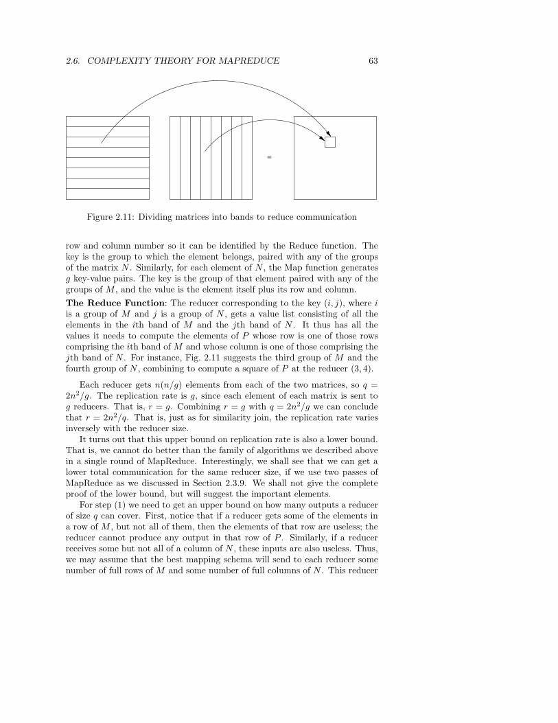
2.6. COMPLEXITY THEORY FOR MAPREDUCE 63
=
Figure 2.11: Dividing matrices into bands to reduce communication
row and column number so it can be identified by the Reduce function. Thekey is the group to which the element belongs, paired with any of the groupsof the matrix N . Similarly, for each element of N , the Map function generatesg key-value pairs. The key is the group of that element paired with any of thegroups of M , and the value is the element itself plus its row and column.
The Reduce Function: The reducer corresponding to the key (i, j), where iis a group of M and j is a group of N , gets a value list consisting of all theelements in the ith band of M and the jth band of N . It thus has all thevalues it needs to compute the elements of P whose row is one of those rowscomprising the ith band of M and whose column is one of those comprising thejth band of N . For instance, Fig. 2.11 suggests the third group of M and thefourth group of N , combining to compute a square of P at the reducer (3, 4).
Each reducer gets n(n/g) elements from each of the two matrices, so q =2n2/g. The replication rate is g, since each element of each matrix is sent tog reducers. That is, r = g. Combining r = g with q = 2n2/g we can concludethat r = 2n2/q. That is, just as for similarity join, the replication rate variesinversely with the reducer size.
It turns out that this upper bound on replication rate is also a lower bound.That is, we cannot do better than the family of algorithms we described abovein a single round of MapReduce. Interestingly, we shall see that we can get alower total communication for the same reducer size, if we use two passes ofMapReduce as we discussed in Section 2.3.9. We shall not give the completeproof of the lower bound, but will suggest the important elements.
For step (1) we need to get an upper bound on how many outputs a reducerof size q can cover. First, notice that if a reducer gets some of the elements ina row of M , but not all of them, then the elements of that row are useless; thereducer cannot produce any output in that row of P . Similarly, if a reducerreceives some but not all of a column of N , these inputs are also useless. Thus,we may assume that the best mapping schema will send to each reducer somenumber of full rows of M and some number of full columns of N . This reducer
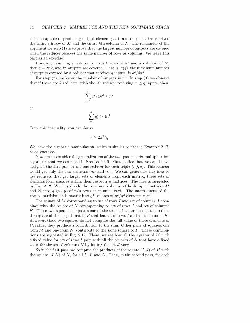
64 CHAPTER 2. MAPREDUCE AND THE NEW SOFTWARE STACK
is then capable of producing output element pik if and only if it has receivedthe entire ith row of M and the entire kth column of N . The remainder of theargument for step (1) is to prove that the largest number of outputs are coveredwhen the reducer receives the same number of rows as columns. We leave thispart as an exercise.
However, assuming a reducer receives k rows of M and k columns of N ,then q = 2nk, and k2 outputs are covered. That is, g(q), the maximum numberof outputs covered by a reducer that receives q inputs, is q2/4n2.
For step (2), we know the number of outputs is n2. In step (3) we observethat if there are k reducers, with the ith reducer receiving qi ≤ q inputs, then
k∑
i=1
q2i /4n2 ≥ n2
ork
∑
i=1
q2i ≥ 4n4
From this inequality, you can derive
r ≥ 2n2/q
We leave the algebraic manipulation, which is similar to that in Example 2.17,as an exercise.
Now, let us consider the generalization of the two-pass matrix-multiplicationalgorithm that we described in Section 2.3.9. First, notice that we could havedesigned the first pass to use one reducer for each triple (i, j, k). This reducerwould get only the two elements mij and njk. We can generalize this idea touse reducers that get larger sets of elements from each matrix; these sets ofelements form squares within their respective matrices. The idea is suggestedby Fig. 2.12. We may divide the rows and columns of both input matrices Mand N into g groups of n/g rows or columns each. The intersections of thegroups partition each matrix into g2 squares of n2/g2 elements each.
The square of M corresponding to set of rows I and set of columns J com-bines with the square of N corresponding to set of rows J and set of columnsK. These two squares compute some of the terms that are needed to producethe square of the output matrix P that has set of rows I and set of columns K.However, these two squares do not compute the full value of these elements ofP ; rather they produce a contribution to the sum. Other pairs of squares, onefrom M and one from N , contribute to the same square of P . These contribu-tions are suggested in Fig. 2.12. There, we see how all the squares of M witha fixed value for set of rows I pair with all the squares of N that have a fixedvalue for the set of columns K by letting the set J vary.
So in the first pass, we compute the products of the square (I, J) of M withthe square (J, K) of N , for all I, J , and K. Then, in the second pass, for each
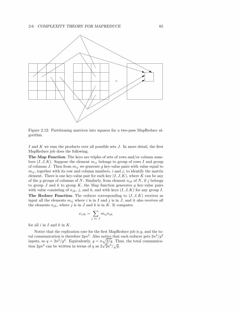
2.6. COMPLEXITY THEORY FOR MAPREDUCE 65
=
Figure 2.12: Partitioning matrices into squares for a two-pass MapReduce al-gorithm
I and K we sum the products over all possible sets J . In more detail, the firstMapReduce job does the following.
The Map Function: The keys are triples of sets of rows and/or column num-bers (I, J, K). Suppose the element mij belongs to group of rows I and groupof columns J . Then from mij we generate g key-value pairs with value equal tomij , together with its row and column numbers, i and j, to identify the matrixelement. There is one key-value pair for each key (I, J, K), where K can be anyof the g groups of columns of N . Similarly, from element njk of N , if j belongsto group J and k to group K, the Map function generates g key-value pairswith value consisting of njk, j, and k, and with keys (I, J, K) for any group I.
The Reduce Function: The reducer corresponding to (I, J, K) receives asinput all the elements mij where i is in I and j is in J , and it also receives allthe elements njk, where j is in J and k is in K. It computes
xiJk =∑
j in J
mijnjk
for all i in I and k in K.
Notice that the replication rate for the first MapReduce job is g, and the to-tal communication is therefore 2gn2. Also notice that each reducer gets 2n2/g2
inputs, so q = 2n2/g2. Equivalently, g = n√
2/q. Thus, the total communica-
tion 2gn2 can be written in terms of q as 2√
2n3/√
q.
66 CHAPTER 2. MAPREDUCE AND THE NEW SOFTWARE STACK
The second MapReduce job is simple; it sums up the xiJk’s over all sets J .
The Map Function: We assume that the Map tasks execute at whatevercompute nodes executed the Reduce tasks of the previous job. Thus, no com-munication is needed between the jobs. The Map function takes as input oneelement xiJk, which we assume the previous reducers have left labeled with iand k so we know to what element of matrix P this term contributes. Onekey-value pair is generated. The key is (i, k) and the value is xiJk.
The Reduce Function: The Reduce function simply sums the values associ-ated with key (i, k) to compute the output element Pik.
The communication between the Map and Reduce tasks of the second job isgn2, since there are n possible values of i, n possible values of k, and g possiblevalues of the set J , and each xiJk is communicated only once. If we recall fromour analysis of the first MapReduce job that g = n
√
2/q, we can write the
communication for the second job as n2g =√
2n3/√
q. This amount is exactlyhalf the communication for the first job, so the total communication for thetwo-pass algorithm is 3
√2n3/
√q. Although we shall not examine this point
here, it turns out that we can do slightly better if we divide the matrices Mand N not into squares but into rectangles that are twice as long on one sideas on the other. In that case, we get the slightly smaller constant 4 in placeof 3
√2 = 4.24, and we get a two-pass algorithm with communication equal to
4n3/√
q.Now, recall that the communication cost we computed for the one-pass
algorithm is 4n4/q. We may as well assume q is less than n2, or else we canjust use a serial algorithm at one compute node and not use MapReduce at all.Thus, n3/
√q is smaller than n4/q, and if q is close to its minimum possible
value of 2n,10 then the two-pass algorithm beats the one-pass algorithm by afactor of O(
√n) in communication. Moreover, we can expect the difference
in communication to be the significant cost difference. Both algorithms dothe same O(n3) arithmetic operations. The two-pass method naturally hasmore overhead managing tasks than does the one-job method. On the otherhand, the second pass of the two-pass algorithm applies a Reduce functionthat is associative and commutative. Thus, it might be possible to save somecommunication cost by using a combiner on that pass.
2.6.8 Exercises for Section 2.6
Exercise 2.6.1 : Describe the graphs that model the following problems.
(a) The multiplication of an n × n matrix by a vector of length n.
(b) The natural join of R(A, B) and S(B, C), where A, B, and C have do-mains of sizes a, b, and c, respectively.
10If q is less than 2n, then a reducer cannot get even one row and one column, and therefore
cannot compute any outputs at all.
2.7. SUMMARY OF CHAPTER 2 67
(c) The grouping and aggregation on the relation R(A, B), where A is thegrouping attribute and B is aggregated by the MAX operation. AssumeA and B have domains of size a and b, respectively.
! Exercise 2.6.2 : Provide the details of the proof that a one-pass matrix-multiplication algorithm requires replication rate at least r ≥ 2n2/q, including:
(a) The proof that, for a fixed reducer size, the maximum number of outputsare covered by a reducer when that reducer receives an equal number ofrows of M and columns of N .
(b) The algebraic manipulation needed, starting with∑k
i=1 q2i ≥ 4n4.
!! Exercise 2.6.3 : Suppose our inputs are bit strings of length b, and the outputscorrespond to pairs of strings at Hamming distance 1.11
(a) Prove that a reducer of size q can cover at most (q/2) log2 q outputs.
(b) Use part (a) to show the lower bound on replication rate: r ≥ b/ log2 q.
(c) Show that there are algorithms with replication rate as given by part (b)for the cases q = 2, q = 2b, and q = 2b/2.
2.7 Summary of Chapter 2
✦ Cluster Computing: A common architecture for very large-scale applica-tions is a cluster of compute nodes (processor chip, main memory, anddisk). Compute nodes are mounted in racks, and the nodes on a rack areconnected, typically by gigabit Ethernet. Racks are also connected by ahigh-speed network or switch.
✦ Distributed File Systems: An architecture for very large-scale file sys-tems has developed recently. Files are composed of chunks of about 64megabytes, and each chunk is replicated several times, on different com-pute nodes or racks.
✦ MapReduce: This programming system allows one to exploit parallelisminherent in cluster computing, and manages the hardware failures thatcan occur during a long computation on many nodes. Many Map tasksand many Reduce tasks are managed by a Master process. Tasks on afailed compute node are rerun by the Master.
✦ The Map Function: This function is written by the user. It takes acollection of input objects and turns each into zero or more key-valuepairs. Keys are not necessarily unique.
11Bit strings have Hamming distance 1 if they differ in exactly one bit position. You may
look ahead to Section 3.5.6 for the general definition.
68 CHAPTER 2. MAPREDUCE AND THE NEW SOFTWARE STACK
✦ The Reduce Function: A MapReduce programming system sorts all thekey-value pairs produced by all the Map tasks, forms all the values asso-ciated with a given key into a list and distributes key-list pairs to Reducetasks. Each Reduce task combines the elements on each list, by applyingthe function written by the user. The results produced by all the Reducetasks form the output of the MapReduce process.
✦ Reducers : It is often convenient to refer to the application of the Reducefunction to a single key and its associated value list as a “reducer.”
✦ Hadoop: This programming system is an open-source implementation of adistributed file system (HDFS, the Hadoop Distributed File System) andMapReduce (Hadoop itself). It is available through the Apache Founda-tion.
✦ Managing Compute-Node Failures: MapReduce systems support restartof tasks that fail because their compute node, or the rack containingthat node, fail. Because Map and Reduce tasks deliver their output onlyafter they finish, it is possible to restart a failed task without concern forpossible repetition of the effects of that task. It is necessary to restart theentire job only if the node at which the Master executes fails.
✦ Applications of MapReduce: While not all parallel algorithms are suitablefor implementation in the MapReduce framework, there are simple im-plementations of matrix-vector and matrix-matrix multiplication. Also,the principal operators of relational algebra are easily implemented inMapReduce.
✦ Workflow Systems : MapReduce has been generalized to systems that sup-port any acyclic collection of functions, each of which can be instantiatedby any number of tasks, each responsible for executing that function ona portion of the data.
✦ Recursive Workflows : When implementing a recursive collection of func-tions, it is not always possible to preserve the ability to restart any failedtask, because recursive tasks may have produced output that was con-sumed by another task before the failure. A number of schemes for check-pointing parts of the computation to allow restart of single tasks, or restartall tasks from a recent point, have been proposed.
✦ Communication-Cost : Many applications of MapReduce or similar sys-tems do very simple things for each task. Then, the dominant cost isusually the cost of transporting data from where it is created to whereit is used. In these cases, efficiency of a MapReduce algorithm can beestimated by calculating the sum of the sizes of the inputs to all thetasks.
2.8. REFERENCES FOR CHAPTER 2 69
✦ Multiway Joins : It is sometimes more efficient to replicate tuples of therelations involved in a join and have the join of three or more relationscomputed as a single MapReduce job. The technique of Lagrangean mul-tipliers can be used to optimize the degree of replication for each of theparticipating relations.
✦ Star Joins : Analytic queries often involve a very large fact table joinedwith smaller dimension tables. These joins can always be done efficientlyby the multiway-join technique. An alternative is to distribute the facttable and replicate the dimension tables permanently, using the samestrategy as would be used if we were taking the multiway join of the facttable and every dimension table.
✦ Replication Rate and Reducer Size: It is often convenient to measurecommunication by the replication rate, which is the communication perinput. Also, the reducer size is the maximum number of inputs associatedwith any reducer. For many problems, it is possible to derive a lowerbound on replication rate as a function of the reducer size.
✦ Representing Problems as Graphs : It is possible to represent many prob-lems that are amenable to MapReduce computation by a graph in whichnodes represent inputs and outputs. An output is connected to all theinputs that are needed to compute that output.
✦ Mapping Schemas : Given the graph of a problem, and given a reducer size,a mapping schema is an assignment of the inputs to one or more reducersso that no reducer is assigned more inputs than the reducer size permits,and yet for every output there is some reducer that gets all the inputsneeded to compute that output. The requirement that there be a mappingschema for any MapReduce algorithm is a good expression of what makesMapReduce algorithms different from general parallel computations.
✦ Matrix Multiplication by MapReduce: There is a family of one-pass Map-Reduce algorithms that performs multiplication of n × n matrices withthe minimum possible replication rate r = 2n2/q, where q is the reducersize. On the other hand, a two-pass MapReduce algorithm for the sameproblem with the same reducer size can use up to a factor of n less com-munication.
2.8 References for Chapter 2
GFS, the Google File System, was described in [10]. The paper on Google’sMapReduce is [8]. Information about Hadoop and HDFS can be found at [11].More detail on relations and relational algebra can be found in [16].
Clustera is covered in [9]. Hyracks (previously called Hyrax) is from [4].The Dryad system [13] has similar capabilities, but requires user creation of
70 CHAPTER 2. MAPREDUCE AND THE NEW SOFTWARE STACK
parallel tasks. That responsibility was automated through the introduction ofDryadLINQ [17]. For a discussion of cluster implementation of recursion, see[1]. Pregel is from [14].
A different approach to recursion was taken in Haloop [5]. There, recursionis seen as an iteration, with the output of one round being input to the nextround. Efficiency is obtained by managing the location of the intermediate dataand the tasks that implement each round.
There are a number of other systems built on a distributed file system and/orMapReduce, which have not been covered here, but may be worth knowingabout. [6] describes BigTable, a Google implementation of an object store ofvery large size. A somewhat different direction was taken at Yahoo! with Pnuts[7]. The latter supports a limited form of transaction processing, for example.
PIG [15] is an implementation of relational algebra on top of Hadoop. Sim-ilarly, Hive [12] implements a restricted form of SQL on top of Hadoop.
The communication-cost model for MapReduce algorithms and the optimalimplementations of multiway joins is from [3]. The material on replication rate,reducer size, and their relationship is from [2]. Solutions to Exercises 2.6.2 and2.6.3 can be found there.
1. F.N. Afrati, V. Borkar, M. Carey, A. Polyzotis, and J.D. Ullman, “Clus-ter computing, recursion, and Datalog,” to appear in Proc. Datalog 2.0Workshop, Elsevier, 2011.
2. F.N. Afrati, A. Das Sarma, S. Salihoglu, and J.D. Ullman, “Upper andlower bounds on the cost of a MapReduce computation.” to appear inProc. Intl. Conf. on Very Large Databases, 2013. Also available as CoRR,abs/1206.4377.
3. F.N. Afrati and J.D. Ullman, “Optimizing joins in a MapReduce environ-ment,” Proc. Thirteenth Intl. Conf. on Extending Database Technology,2010.
4. V. Borkar and M. Carey, “Hyrax: demonstrating a new foundation fordata-parallel computation,”
http://asterix.ics.uci.edu/pub/hyraxdemo.pdf
Univ. of California, Irvine, 2010.
5. Y. Bu, B. Howe, M. Balazinska, and M. Ernst, “HaLoop: efficient iter-ative data processing on large clusters,” Proc. Intl. Conf. on Very LargeDatabases, 2010.
6. F. Chang, J. Dean, S. Ghemawat, W.C. Hsieh, D.A. Wallach, M. Burrows,T. Chandra, A. Fikes, and R.E. Gruber, “Bigtable: a distributed storagesystem for structured data,” ACM Transactions on Computer Systems26:2, pp. 1–26, 2008.
2.8. REFERENCES FOR CHAPTER 2 71
7. B.F. Cooper, R. Ramakrishnan, U. Srivastava, A. Silberstein, P. Bohan-non, H.-A. Jacobsen, N. Puz, D. Weaver, and R. Yerneni, “Pnuts: Ya-hoo!’s hosted data serving platform,” PVLDB 1:2, pp. 1277–1288, 2008.
8. J. Dean and S. Ghemawat, “Mapreduce: simplified data processing onlarge clusters,” Comm. ACM 51:1, pp. 107–113, 2008.
9. D.J. DeWitt, E. Paulson, E. Robinson, J.F. Naughton, J. Royalty, S.Shankar, and A. Krioukov, “Clustera: an integrated computation anddata management system,” PVLDB 1:1, pp. 28–41, 2008.
10. S. Ghemawat, H. Gobioff, and S.-T. Leung, “The Google file system,”19th ACM Symposium on Operating Systems Principles, 2003.
11. hadoop.apache.org, Apache Foundation.
12. hadoop.apache.org/hive, Apache Foundation.
13. M. Isard, M. Budiu, Y. Yu, A. Birrell, and D. Fetterly. “Dryad: dis-tributed data-parallel programs from sequential building blocks,” Proceed-ings of the 2nd ACM SIGOPS/EuroSys European Conference on Com-puter Systems, pp. 59–72, ACM, 2007.
14. G. Malewicz, M.N. Austern, A.J.C. Sik, J.C. Denhert, H. Horn, N. Leiser,and G. Czajkowski, “Pregel: a system for large-scale graph processing,”Proc. ACM SIGMOD Conference, 2010.
15. C. Olston, B. Reed, U. Srivastava, R. Kumar, and A. Tomkins, “Pig latin:a not-so-foreign language for data processing,” Proc. ACM SIGMOD Con-ference, pp. 1099–1110, 2008.
16. J.D. Ullman and J. Widom, A First Course in Database Systems, ThirdEdition, Prentice-Hall, Upper Saddle River, NJ, 2008.
17. Y. Yu, M. Isard, D. Fetterly, M. Budiu, I. Erlingsson, P.K. Gunda, andJ. Currey, “DryadLINQ: a system for general-purpose distributed data-parallel computing using a high-level language,” OSDI, pp. 1–14, USENIXAssociation, 2008.