DIgSILENT Pacific PowerFactory Technical Seminar

1

Topic: The Wonders of Optimal Power FlowPresenter: Wayne OngVenue: Sydney Novotel Central / Brisbane Marriott HotelDate: 16th and 30th November 2017

Agenda – The Wonders of Optimal Power Flow

• Ponderings

– From an investor’s view

– From a system operator’s view

• Optimal Power Flow

– Objective function

– Network constraints

– Set of controls

– Calculation methods

• Demonstration

– Solar farm connection

– Power system operator

2

Question #1 – Investor

3

• Investor – If I build a generator at location X, how much money can I expect to make per year?

Question #1 – Investor

4

• Investor – If I build a generator at location X, how much money can I expect to make per year?

• Answer depends on:

1. Available energy resource

2. Available transmission capacity

• Ability to evacuate MW to the market

• Marginal Loss Factors

3. Price for energy ($ / MWh)

Transmission capacity restricting generation – not considering contingencies

5

G1 maximum

generation is

170 MW

Transmission capacity restricting generation – considering contingencies

6

G1 maximum

generation is

91 MW

Question #2 – System operator

7

• System operator – Can I re-dispatch generation in the grid to reduce fuel costs?

Question #2 – System operator

8

• System operator – Can I re-dispatch generation in the grid to reduce fuel costs?

• Answer depends on:

1. Mix of generation sources

2. Transmission capacity

3. Security criteria

In an electricity market (such as the NEM) the market should (theoretically) minimise generation costs

Dispatch A – $77/MWh

9

Dispatch B – $63/MWh

10

Question #3 – System operator

11

• System operator – Can I better operate my system to reduce losses?

Question #3 – System operator

12

• System operator – Can I better operate my system to reduce losses?

• Losses are proportional to I2

• Answer depends on:

1. Ability to control current flows in the system

Losses A – 5.88 MW

13

Losses B – 5.58 MW

14

How can these questions be answered?

15

• Optimal Power Flow (OPF) simulation

– An OPF function schedules the power system controls to optimise an objective function while satisfying system constraints.

– Essentially a load flow solution for a given set of demands and a given set of generation that can be dispatched to meet these demands.

Optimal Power Flow

16

• Objective function to optimisation, i.e. fuel costs, system losses

• Network constraints the solution is subjected to,i.e. valid load-flow, system and equipment limits, operating and security limits

• Set of controls to modify the solution,i.e. generator dispatch, power system controls

Typical OPF configuration

17

• Objective Function: Costs

– Control: Active Power

– Constraints: Branch Flow and Active Power limits

• Objective Function: Losses

– Control: Reactive Power

– Constraint: Reactive Power limits and Voltage limits

OPF calculation methods in PowerFactory

18

• AC Optimisation (Interior Point Method)

– Based on AC load flow

– Non-Linear Constrained Optimisation Problem

• Solves for voltages (angles, magnitudes), and active/reactive power flows

• Requires iterative method

• DC Optimisation (Linear Programming (LP))

– Based on DC load flow

– Linear Constrained Optimisation Problem

• Solves for voltage angles, and active power flows (voltage magnitude fixed at 1.0 pu)

• No iterative method required

• Contingency Constrained DC Optimisation (LP)

– Subject to the constraints imposed by a set of selected contingencies

DEMONSTRATION

19

Example #1 – New NSW solar farm connection

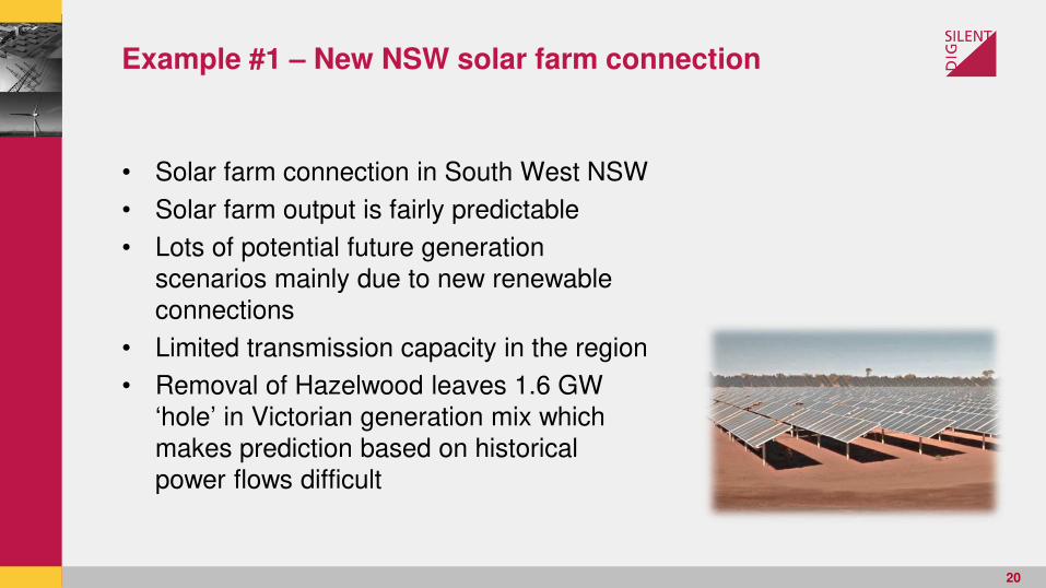
• Solar farm connection in South West NSW

• Solar farm output is fairly predictable

• Lots of potential future generation scenarios mainly due to new renewable connections

• Limited transmission capacity in the region

• Removal of Hazelwood leaves 1.6 GW ‘hole’ in Victorian generation mix which makes prediction based on historical power flows difficult

20

NSW solar farm connection - process

1. Determine hourly demand at grid interface points using AEMO system snapshots

2. Analyse historical outputs of generators to develop cost curves ($/MW)

3. Develop model of the NEM in PowerFactory with variations capturing possible future generation expansion scenarios (including removal of Hazelwood Power Station)

4. Calculate OPF for each hour of the year, with objective of minimising costs and calculate MW output constrained for the proposed solar farm

21

DEMONSTRATION

22

Example #2 – Power system operator – reduce fuel costs

• Developing country grid operator with high cost of generation

– Heavy fuel oil plant run as base load generation

• Electrical demand growth

– Exceeds 10% per annum

• To quantify cost of inefficient generation dispatch

– Drive dispatch efficiency improvement projects

• Future generation development affects utilisation of transmission infrastructure

– To verify that transmission plan is economically sound

(for most likely future scenarios)

23

Generation dispatch & transmission planning - process

1. Determine several demand scenarios (taken from yearly load duration curve) for target future years

2. Analyse fuel cost data and convert to electrical operating cost ($/MWh)

3. Develop model of the system in PowerFactory with variations capturing possible future generation and transmission expansion scenarios

4. Calculate OPF for each demand scenario, with objective of minimising costs

5. Analyse equipment (lines and transformers) that are operating at thermal limits and are underutilised across expansion and demand scenarios

24

0

0.1

0.2

0.3

0.4

0.5

0.6

0.7

0.8

0.9

1

0 1000 2000 3000 4000 5000 6000 7000 8000 9000 10000

Hours

Normalised load duration curve

0.81

0.69

0.55

0.41

30%

30%

30%

5%

5%

Power system model

• Geographic coordinates

– Substations

– Lines

• Plant operating costs

• Generation plan up to 2025

25

Unconstrained dispatch

• The diameter corresponds to the magnitude at each site for

– Generation – purple circles

– Load – blue circle

• Figure shows 92.5% peak demand 2016

26

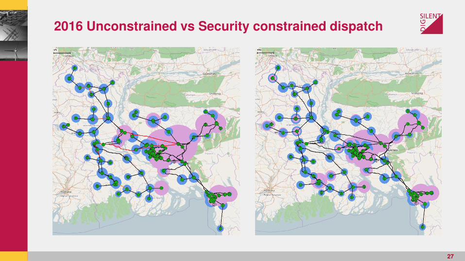
2016 Unconstrained vs Security constrained dispatch

27

2025 Unconstrained vs Security constrained dispatch

28

QUESTIONS

Thank you

29