digital image processing prof. p. k. biswas …textofvideo.nptel.ac.in/117105135/lec3.pdf · we...
TRANSCRIPT

Digital Image Processing Prof. P. K. Biswas
Department of Electronics and Electrical Communications Engineering Indian Institute of Technology, Kharagpur
Module 01 Lecture Number 03 Image Digitalization, Sampling Quantization and Display
(Refer Slide Time 00:17)
Welcome to the course on Digital Image Processing.
(Refer Slide Time 00:21)

We will also talk about what is meant by signal bandwidth. We will talk about how to select
the sampling frequency of a given signal, and we will also see the image reconstruction
process from the sampled values.
(Refer Slide Time 00:42)
So in today's lecture, we will try to find out the answers to 3 basic questions. The first
question is why do we need digitization? Then we will try to find the answer to what is meant
by digitization and thirdly, we will go to how to digitize an image.
(Refer Slide Time 01:07)
So let us talk about this one after another. Firstly, let us see that why image digitization is
necessary.
(Refer Slide Time 01:17)
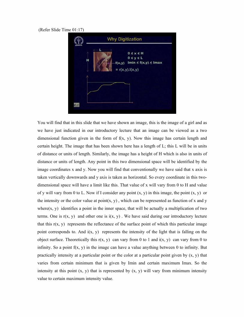
You will find that in this slide that we have shown an image, this is the image of a girl and as
we have just indicated in our introductory lecture that an image can be viewed as a two
dimensional function given in the form of f(x, y). Now this image has certain length and
certain height. The image that has been shown here has a length of L; this L will be in units
of distance or units of length. Similarly, the image has a height of H which is also in units of
distance or units of length. Any point in this two dimensional space will be identified by the
image coordinates x and y. Now you will find that conventionally we have said that x axis is
taken vertically downwards and y axis is taken as horizontal. So every coordinate in this two-
dimensional space will have a limit like this. That value of x will vary from 0 to H and value
of y will vary from 0 to L. Now if I consider any point (x, y) in this image, the point (x, y) or
the intensity or the color value at point(x, y) , which can be represented as function of x and y
where(x, y) identifies a point in the inner space, that will be actually a multiplication of two
terms. One is r(x, y) and other one is i(x, y) . We have said during our introductory lecture
that this r(x, y) represents the reflectance of the surface point of which this particular image
point corresponds to. And i(x, y) represents the intensity of the light that is falling on the
object surface. Theoretically this r(x, y) can vary from 0 to 1 and i(x, y) can vary from 0 to
infinity. So a point f(x, y) in the image can have a value anything between 0 to infinity. But
practically intensity at a particular point or the color at a particular point given by (x, y) that
varies from certain minimum that is given by Imin and certain maximum Imax. So the
intensity at this point (x, y) that is represented by (x, y) will vary from minimum intensity
value to certain maximum intensity value.

Now you will find the second figure in this particular slide. It shows that if I take a horizontal
line on this image space and if I plot intensity values along that line, the intensity profile will
be something like this. It again shows that this is the minimum intensity value along that line
and this is the maximum intensity value along the line. So the intensity at any point in the
image or intensity along a line whether it is horizontal or vertical, can assume any value
between the maximum and the minimum.
Now here lies the problem. When we consider a continuous image which can assume any
value, an intensity can assume any value between certain minimum and certain maximum and
the coordinate points x and y they can also some value between, x can vary from 0 to H, y
can vary from 0 to L.
(Refer Slide Time 05:10)
Now from the Theory of Real Numbers, you know that given any two points, that is, between
any two points there are infinite numbers of points. So again when I come to

(Refer Slide Time 05:21)
this image, as x varies from 0 to H, there can be infinite possible values of x between 0 and
H. Similarly, there can be infinite values of y between 0 and L. So effectively
(Refer Slide Time 05:39)
that means that if I want to represent
(Refer Slide Time 05:42)
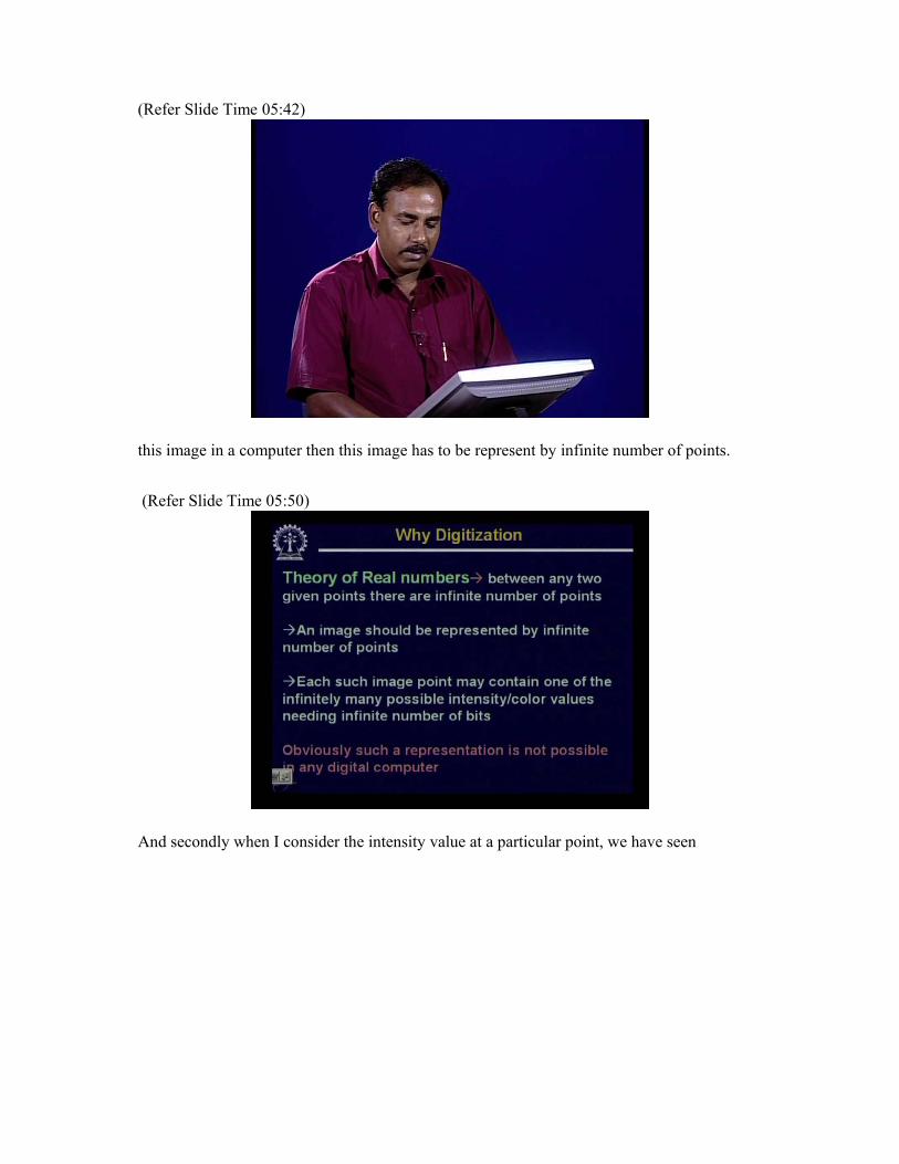
this image in a computer then this image has to be represent by infinite number of points.
(Refer Slide Time 05:50)
And secondly when I consider the intensity value at a particular point, we have seen

(Refer Slide Time 05:56)
that the intensity value f(x, y) it varies between certain minimum “Imin” and certain
maximum “Imax”. Again if I take these two “Imin” and “Imax” to be minimum and
maximum intensity values possible
(Refer Slide Time 06:17)
but here again the problem is the intensity values, the number of intensity values that can be
between minimum and maximum is again infinite in number; so which again means that if I
want to represent an intensity value in a digital computer then I have to have infinite number
of bits to represent an intensity value. And obviously such a representation is not possible in
any digital computer.

So naturally we have to find out a way out,
(Refer Slide Time 06:50)
that is our requirement is we have to represent this image in a digital computer in a digital
form. So what is the way out? In our introductory lecture, if you remember that we have said
that instead of considering every possible point in the image space, we will take some
discrete set of points and those discrete set of points are decided by grid. So if we have a
uniform rectangular grid, then at each of the grid locations we can take a particular point and
we will consider the intensity at that particular point. So this is a process which is known as
sampling.
(Refer Slide Time 07:31)

So what is desired is we want that an image should be represented in a form of finite two-
dimensional matrix like this. So this is a matrix representation of an image and this matrix
has got finite number of elements. So if you look at this matrix, you find that this matrix has
got m number of rows, varying from 0 to m minus 1 and the matrix has got n number of
columns, varying from 0 to n minus 1. Typically for image processing applications we have
mentioned that the dimension is usually taken either as 256 x 256 or 512 x 512 or 1 K x 1 K
and so on. But still whatever be the size, the matrix is still finite. We have finite number of
rows and we have finite number of columns. So after sampling what we get is an image in the
form of a matrix like this.
Now the second requirement is, if I don't do any other processing on these matrix elements,
now what this matrix element represents? Every matrix element represents an intensity value
in the corresponding image location. And we have said that these intensity values or the
number of intensity values can again be infinite between certain minimum and maximum
which is again not possible to be represented in a digital computer. So here what we want is
each of the matrix elements should also assume one of finite discrete values. So when I do
both of these,
(Refer Slide Time 09:18)
that is first operation is sampling to represent the image in the form of a finite two-
dimensional matrix and each of the matrix elements again has to be digitized so that the
intensity value at a particular element or a particular element in a matrix can assume only

values from a finite set of discrete values. These two together completes the image
digitization process.
Now here is an example.
(Refer Slide Time 09:47)
You find that we have shown an image on the left hand side and if I take a small rectangle in
this image and try to find out what are the values in that small rectangle, you find that these
values are in the form of a finite matrix and every element in this rectangular, in this small
rectangle or in this small matrix assumes an integer value. So an image when it is digitized
will be represented in the form of a matrix like this.
(Refer Slide Time 10:23)

So typically what we have said till now, it indicates that by digitization what we mean is an
image representation by a 2D, two-dimensional finite matrix, the process known as sampling
and the second operation is each matrix element must be represented by one of the finite set
of discrete values and this is an operation which is called quantization. In today's lecture
(Refer Slide Time 10:56)
we will mainly concentrate on the sampling; and quantization we will talk about later.
Now let us see that how,
(Refer Slide Time 11:11)
what should be the different blocks in an image processing system. Firstly, we have seen that
computer processing of images requires that images be available in digital form and so we
have to digitize the image. And the digitization process is a two-step process. The first step is

sampling and the second step is quantization. Then finally when we digitize an image
processed by computer, then obviously our final aim will be that we want to see
(Refer Slide Time 11:51)
that what is the processed output
So we have to display the image on a display device. Now when then image has been
processed, the image in the digital form but when we want to have the display, we must have
the display in the form of analog. So whatever process we have done during digitization,
during visualization or during display, we must do the reverse process. So for displaying the
images, it is, it has to be first converted into the analog signal which is then displayed on a
normal display. So if we just look in the form of a block diagram
(Refer Slide Time 12:31)

it appears something like this.
That while digitization, first we have to sample the image by a unit which is known as
sampler, then every sampled values we have to digitize, the process known as quantization
and after quantization
(Refer Slide Time 12:49)
we get a digital image which is processed by the digital computer.
And when we want to see the processed image that is how does the image look like after the
processing is complete then for that operation it is the digital computer which gives the
digital output.
(Refer Slide Time 13:13)

This digital output goes to D to A converter and finally the digital to analog converter output
is fed to the display and on the display we can see that how the processed image looks like.
(Refer Slide Time 13:25)
Now
(Refer Slide Time 13:29)
let us come to the first step of the digitization process that is sampling. To understand
sampling, before going to the two-dimensional image let us take an example from one
dimension. That is, let us assume that we have a one-dimensional signal x(t) which is a
function of t. Here we assume this t to be time and you know that whenever some signal is
represented as a function of time, whatever is the frequency content of the signal that is
represented in the form of Hz and this Hz means it is cycles per unit time. So here again,
when you look at this particular signal x(t), you find that this is an analog signal that is t can
assume any value, t is not discretized. Similarly, the functional value x(t) can also assume any
value between certain maximum and minimum. So obviously this is an analog signal and we
have seen that an analog signal cannot be represented in a computer. So what is the first step
that we have to do? As we said, for the digitization process, the first operation that you have
to do is the sampling operation.
So for sampling what we do is
(Refer Slide Time 14:55)
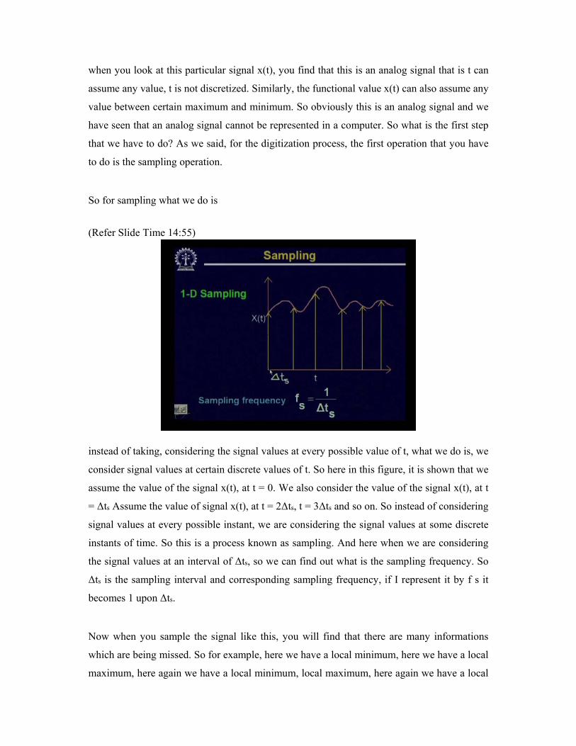
instead of taking, considering the signal values at every possible value of t, what we do is, we
consider signal values at certain discrete values of t. So here in this figure, it is shown that we
assume the value of the signal x(t), at t = 0. We also consider the value of the signal x(t), at t
= Δts Assume the value of signal x(t), at t = 2Δts, t = 3Δts and so on. So instead of considering
signal values at every possible instant, we are considering the signal values at some discrete
instants of time. So this is a process known as sampling. And here when we are considering
the signal values at an interval of Δts, so we can find out what is the sampling frequency. So
Δts is the sampling interval and corresponding sampling frequency, if I represent it by f s it
becomes 1 upon Δts.
Now when you sample the signal like this, you will find that there are many informations
which are being missed. So for example, here we have a local minimum, here we have a local
maximum, here again we have a local minimum, local maximum, here again we have a local

maximum and when we sample at an interval of Δts, these are the informations that cannot be
captured by these samples. So what is the alternative?
(Refer Slide Time 16:39)
The alternative is let us increase the sampling frequency or let us decreasing the sampling
interval. So if I do that you will find that these bold lines, bold golden lines
(Refer Slide Time 16:55)
they represent the earlier samples that we had, like this

(Refer Slide Time 17:00)
whereas these dotted green lines, they represent the new samples that we want to take. And
when we take the new samples, what we do is we reduce the sampling interval by half. That
is our earlier sampling interval was Δts, now I make the new sampling interval which I
represent as Δts’ = Δts/2; and obviously in this case, the sampling frequency which is fs
’ =
1/Δts’, now it becomes twice of fs. That is, earlier we had the sampling frequency of fs, now
we have the sampling frequency of 2fs, twice fs. And when you increase the sampling
frequency, you find that with the earlier samples represented by this solid lines you find that
this particular information that is tip in between these two solid lines were missed. Now when
I introduce a sample in between, then some information of this minimum or of this local
maximum can be retained. Similarly, here, some information of this local minimum can also
be retained. So obviously it says that when I increase the sampling frequency or I reducing
the sampling interval

(Refer Slide Time 18:24)
then the information that I can maintain in the sampled signal will be more than when the
sampling frequency is less. Now the question comes, whether there is a theoretical
background by which we can decide that what is the sampling frequency, proper sampling
frequency for certain signals, that we can decide. We will come to that a bit later.
Now let us see that what does this sampling actually mean?
(Refer Slide Time 18:58)
We have seen that we have a continuous signal x(t) and for digitization instead of considering
the signal values at every possible value of t, we have considered the signal values at some
discrete instants of time t, Ok. Now this particular sampling process can be represented

(Refer Slide Time 19:16)
mathematically in the form that if I have, if I consider that I have a sampling function and this
sampling function is one-dimensional array of Dirac delta functions which are situated at a
regular spacing of Δt. So this sequence of Dirac delta functions can be represented in this
form. So you find that each of these are sequence of Dirac delta functions and the spacing
between two functions is Δt. In short, these kind of function is represented by comb function,
a comb function t at an interval of Δt and mathematically this comb function can be
represented as comb(t;Δt) (t-mΔt).m
m
Now this is the Dirac delta function. The Dirac delta function says that if I have a Dirac delta
function Δt then the functional value will be 1, whenever t = 0 and the functional value will
be 0 for all other values of t. In this case when I have Δt- mΔt, then this functional value will
be 1 only when this quantity, that is, t – mΔt, = 0. That means this functional value will
assume a value 1 whenever t = mΔ t for different values of m varying from -∞ to ∞.
So effectively this mathematical expression gives rise to a series of Dirac delta functions in
this form where at an interval of Δt, I get a value of 1. For all other values of t, I get values of
0. Now this sampling

(Refer Slide Time 21:14)
as you find that we have represented the same figure here, we had this continuous signal x(t),
original signal. After sampling we get a number of samples like this. Now here, these samples
can now be represented by multiplication of x(t) with the series of Dirac delta functions that
you have seen, that is, comb(t; Δt). So if I multiply this, whenever this comb function gives
me a value 1, only the corresponding value of t will be retained in the product and whenever
this comb function gives you a value 0, the corresponding points, the corresponding values of
x(t) will be set to 0. So effectively, this particular sampling, when from this analog signal,
this continuous signal, we have gone to this discrete signal, this discretization process can be
represented mathematically as sX (t)=X(t).comb(t,Δt) and if I expand this comb function and
consider only the values of t, where this comb function has a value 1, then this mathematical
expression is translated m=¥
s
m=-¥
X (t)= X(mΔt) (t-mΔt) , right.

(Refer Slide Time 22:43)
So after sampling what you have got is, from a continuous signal we have got the sampled
signal represented by Xs(t) where the sample values exist at discrete instants of time.
Sampling, what we get is a sequence of samples as shown in this figure where Xs(t) has got
the signal values at discrete time instants and during the other time intervals, the value of the
signal is set to 0. Now this sampling will be proper if we are able to reconstruct the original,
continuous signal x(t) from these sample values. And you will find out that while sampling
we have to maintain certain conditions so that the reconstruction of the analog signal x(t) is
possible.
(Refer Slide Time 23:47)

Now let us look at some mathematical background which will help us to find out the
conditions which we have to impose for this kind of reconstruction. So here you find that if
we have a continuous signal in time which is represented by x(t)
(Refer Slide Time 24:21)
then we know that the frequency components of this signal x(t) can be obtained by taking the
Fourier transform of this x(t). So if I take the Fourier transform of x(t) which is represented
by F{x(t)}, which is also represented in the form of X(ω), where ω is the frequency
component and mathematically this will be represented as -jωtF{x(t)}= x(t)e dt
. So this
mathematical expression gives us the frequency components which is obtained by the
(Refer Slide Time 25:24)

Fourier transform of the signal x(t). Now this is possible if the signal x(t) is aperiodic. But
when the signal x(t) is periodic, in that case the instead of taking the Fourier transform, we
have to go for Fourier series expansion. And the Fourier series expansion of a periodic signal
say v(t)
(Refer Slide Time 25:52)
where we assume that v(t) is a periodic signal, is given by this expression
where ω0 is the fundamental frequency of this signal v(t)
(Refer Slide Time 26:23)
and we have to take the summation from
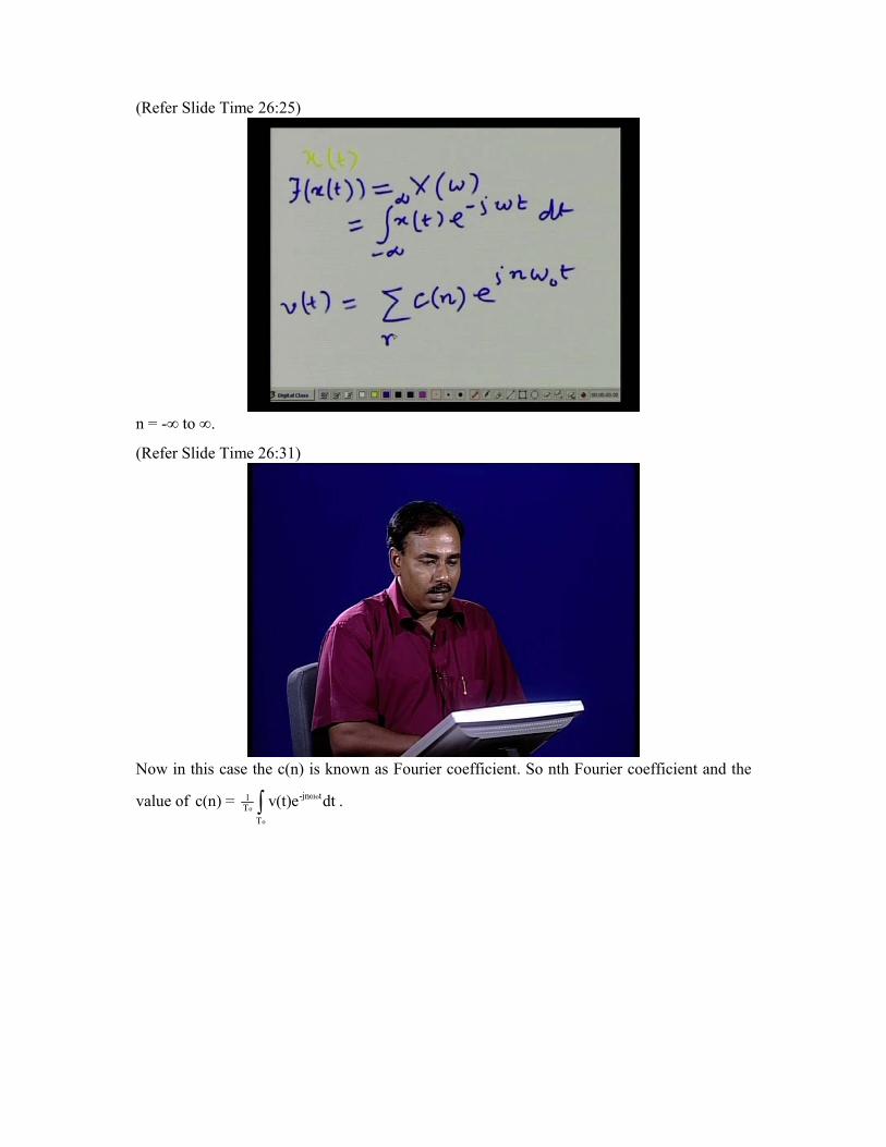
(Refer Slide Time 26:25)
n = -∞ to ∞.
(Refer Slide Time 26:31)
Now in this case the c(n) is known as Fourier coefficient. So nth Fourier coefficient and the
value of o
o
o
-jnω t1T
T
c(n) = v(t)e dt .

(Refer Slide Time 26:46)
Now in our case when we have this v(t) in the form of series of Dirac delta functions, in that
case we know
(Refer Slide Time 27:24)
we know that value of v(t) will be = 1; when t = 0 and value of v(t) is = 0 for any other value
of t within a single period.
So in our case
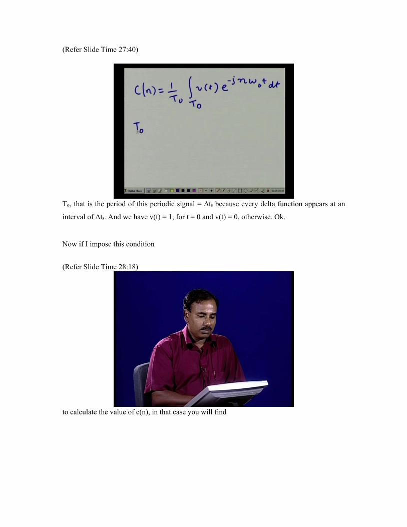
(Refer Slide Time 27:40)
To, that is the period of this periodic signal = Δts because every delta function appears at an
interval of Δts. And we have v(t) = 1, for t = 0 and v(t) = 0, otherwise. Ok.
Now if I impose this condition
(Refer Slide Time 28:18)
to calculate the value of c(n), in that case you will find

(Refer Slide Time 28:23)
that the value of this integral will exist only at t = 0 and it will be 0 for
(Refer Slide Time 28:28)
any other value of t So by this we find that c(n), now

(Refer Slide Time 28:35)
Becomes, c(n) = 1/Δts and this is nothing, but the sampling frequency we put at, say ωs. So
this is the frequency of the sampling signal.
(Refer Slide Time 28:52)
Now with this value of c(n), now the periodic signal

(Refer Slide Time 28:57)
v(t) can be represented as 1( ) ot
s
jnT
n
v t e
. So what does it mean? This means that if I take
the Fourier series expansion of our periodic signal which is in our case Dirac delta function,
this will have frequency components
(Refer Slide Time 29:33)
various frequency components for the fundamental component of frequency is ωo and it will
have other frequency components of 2ωo, 3ωo, 4ωo and so on.

(Refer Slide Time 29:50)
So if I plot those frequencies or frequency spectrum we find that will have the fundamental
frequency ωo naught or in this case, this ωo is nothing but same as the sampling frequency ωs.
We will also have a frequency component of 2ωs, we will also have a frequency component
of 3ωs and this continues like this. So you will find that the comb function as the sampling
function
(Refer Slide Time 30:22)
that we have taken, the Fourier series expansion of that is again a comb function. Now this is
about the continuous domain.
When you go to discrete domain, in that case,

(Refer Slide Time 30:38)
for a discrete time signal say x(n) where n is the nth sample of the signal x(n), the Fourier
Transform of this is given by 2πN
N-1-j( )nk
n=0
X(k)= x(n)e , where value of n varies from 0 to N-1,
where this N indicates number of samples that we have for which we are taking the Fourier
transform. And given this Fourier Transform, we can find out the original sampled signal by
the inverse Fourier transformation which is obtained as 2πN
N-1j( )nk
k=0
x(n)= X(k)e . So you find that
we get a Fourier Transform pair, in one case from the discrete time signal, we get the
frequency component, discrete frequency components by the forward Fourier transform and
in the second case, from the frequency components, we get the discrete time signal by the
inverse Fourier transform. And these two equations taken together form a Fourier Transform
pair.

(Refer Slide Time 32:32)
Now let us go to another concept.
(Refer Slide Time 32:34)
Thank you.