process integration prof. bikash mohanty department of...

Process Integration Prof. Bikash Mohanty

Department of Chemical Engineering Indian Institute of Technology, Roorkee

Module - 2

Fundamental Concepts Lecture - 2

Fundamental Concepts Related to Heat Integration – Part 02

We have already discussed what is the F T factor? And how it takes into account the

different flow patterns inside a shell and tube heat exchanger.

(Refer Slide Time: 00:54)

Now the F T factors can be expressed in different expressions like given here. The

expression for F T for a 1-2 heat exchanger that is one shell, two-tube side heat

exchanger is as follows for R is equal to 1, the F T factor is written in the screen and for

R is equal to 1 that is another expression. So, we have two expressions R not equal to 1,

and R equal to 1. Now, what are the salient features of this F T diagram. If you see this F

T diagram, the y-axis is F T and the x-axis is P, and these F T plots are drawn for

different values of R. It is R is 10.0, this is R is 2.0, this is R here R is 0.5. Now we see

that for certain area, this F T factor is properly expressing the value of F T, but after that

the slope becomes very steep.

So, from the diagram, it can be seen that with the decreasing F T, the slope of F T curve

for a given value of R becomes very steep like in this range, very steep. In this range, it

is very steep; in this range, it is very steep; in this range, it is steep; in this range, it is

steep, and approaches to a certain value of p asymptotically. So, if this is a line, we see

that this approaches to this line when F moves to the infinite values, so here we see that

up to 0.75 this is a rough estimate we can measure the F T values properly, but after that

the slope becomes very steep. So, this is the red area is called the infeasible area, and the

green area is called the feasible area; that means, when designing a heat exchanger, we

will always try to be in green area.


Three basic situations, which are encountered while using 1-2 shell and tube heat

exchanger, and for that let us explain what is temperature approach? The final

temperature of the hot stream is higher than the final temperature of the cold stream as

shown here. This is the point is the final temperature of the cold stream and this point is

the final temperature of the hot stream. In the F T diagram, if we want to represent this

yet this is the scenario, in the F T diagram, we will have a F T somewhere here in the

feasible region, this is called the temperature approach because this temperature is

approaching this temperature. This is called temperature approach - as outlet temperature

of the hot stream approaches to the outlet temperature of the cold stream. This situation

is straight forward to design, since it can always be accommodated in a 1-2 shell and

tube heat exchanges, and the F T value somewhere fall in this region.


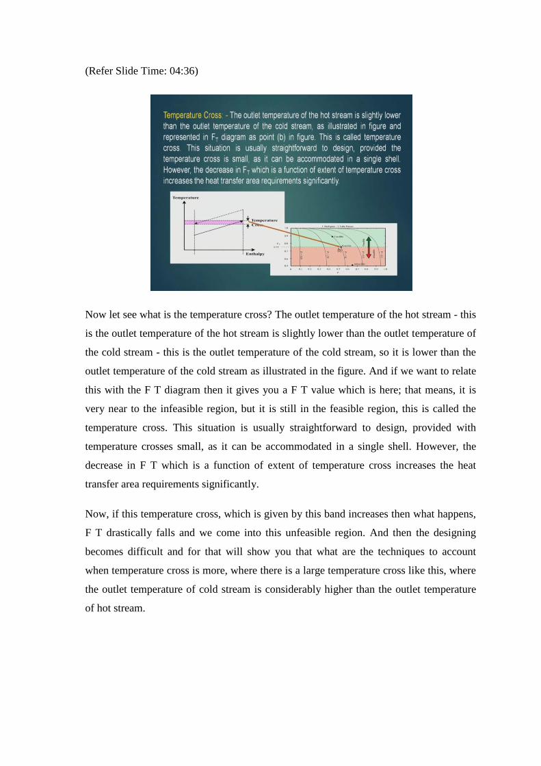
Now let see what is the temperature cross? The outlet temperature of the hot stream - this

is the outlet temperature of the hot stream is slightly lower than the outlet temperature of

the cold stream - this is the outlet temperature of the cold stream, so it is lower than the

outlet temperature of the cold stream as illustrated in the figure. And if we want to relate

this with the F T diagram then it gives you a F T value which is here; that means, it is

very near to the infeasible region, but it is still in the feasible region, this is called the

temperature cross. This situation is usually straightforward to design, provided with

temperature crosses small, as it can be accommodated in a single shell. However, the

decrease in F T which is a function of extent of temperature cross increases the heat

transfer area requirements significantly.

Now, if this temperature cross, which is given by this band increases then what happens,

F T drastically falls and we come into this unfeasible region. And then the designing

becomes difficult and for that will show you that what are the techniques to account

when temperature cross is more, where there is a large temperature cross like this, where

the outlet temperature of cold stream is considerably higher than the outlet temperature

of hot stream.


And if you relate this to the F T curve then we find that it falls somewhere here in the

infeasible region. In this case, the F T decreases significantly, causing the dramatic

increase in the heat transfer area requirement leading to an infeasible design. Local

reversal of heat flow may also be encountered, which is wasteful in heat transfer area.

Thus, for a given R the design of the heat exchanger becomes less and less efficient as a

asymptotic region of the F T curve is reached. So, we will not like to design a heat

exchanger in this asymptotical region, because this may lead to instability.


The maximum temperature cross that can be tolerated is often set by a thumb rule, for

example, F T greater than 0.75. And we have seen that we have drawn this line to

demarcate infeasible and feasible region, it is important to avoid low values of F T

because low values of F T indicate inefficient use of heat transfer area. Any uncertainties

inaccuracies designed data will significantly affect the design of the heat exchanger

when design is carried out in the area where F T slopes are steep. Further, operation of

heat exchanger in this area will be unpredictable.

Consequently, to be confident in design, those part of the F T chart where slope are steep

should be avoided, even if F T is greater than 0.75. A simple method to achieve this is

based upon the fact that for any value of R there is a maximum asymptotic value P, say P

max, which is achieved when F T tends to negative infinity as shown in this figure, and

is obtained as follows. Now when this F T curve we see when it reaches to minus

infinite, this R asymptotically reaches to a P max value now we will see some derivation

that how to compute this P max value and to find out a value of P, which will not put us

in this region of design.


Now according to the bowman et al for R is not equal to one, this is the expression of the

F T. And for the R is equal to one, this is the expression. The maximum value of P for

any R occurs as F T tends to negative infinite that we have seen in the earlier figure,

from the F T functions above for F T to be determinate the p should be less than one.

Because if p is less than one then the term inside the l n will not be negative and hence

we would be able to compute the F T. For the R p multiplication should be less than one

for this factor which is two minus p in brackets R plus one minus root over R square plus

one divided by 2 minus P R plus 1 plus root over R square plus 1 should be greater than

0. So, these are the three conditions, and let us analyze one by one these conditions. The

condition three applies when R is equal to 1. Both conditions one and two are always

true for feasible heat exchange with positive temperature difference.


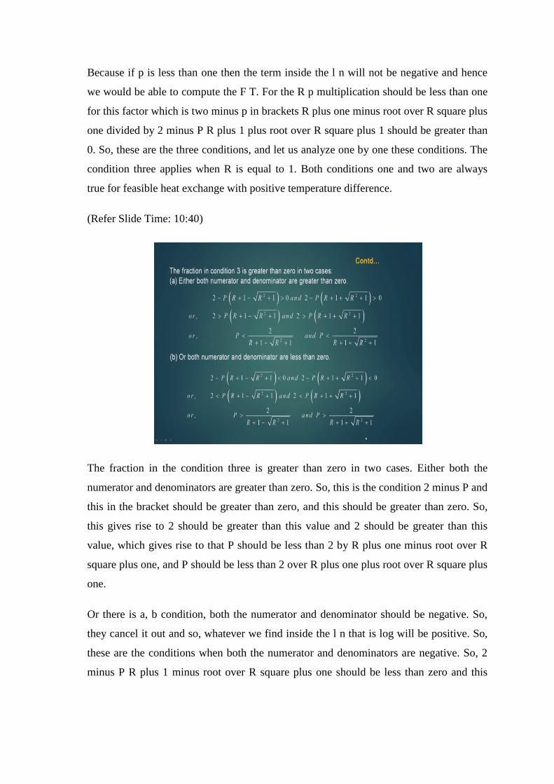
The fraction in the condition three is greater than zero in two cases. Either both the

numerator and denominators are greater than zero. So, this is the condition 2 minus P and

this in the bracket should be greater than zero, and this should be greater than zero. So,

this gives rise to 2 should be greater than this value and 2 should be greater than this

value, which gives rise to that P should be less than 2 by R plus one minus root over R

square plus one, and P should be less than 2 over R plus one plus root over R square plus

one.

Or there is a, b condition, both the numerator and denominator should be negative. So,

they cancel it out and so, whatever we find inside the l n that is log will be positive. So,

these are the conditions when both the numerator and denominators are negative. So, 2

minus P R plus 1 minus root over R square plus one should be less than zero and this

should be less than zero. So, this gives rise to a condition that P should be greater than 2

divided by R plus 1 minus root over R square plus 1 and P should be greater than this.


So, let us now closely examine these two conditions. For condition 3, either a or b are

true, but not both. Let us consider the condition b in more detail. For positive value of R,

R plus 1 minus root over R square plus 1 is a continuously increasing function of R and

as R tends to 0, this value R plus 1 minus root over R square plus 1 will tend to zero.

And as R tends to infinite, this tends to one; that means, if I move from zero to infinite,

the maximum value which I will get for this factor will be one and minimum value zero.

And if it is within this zero to infinite then the value will be less than one. For

determination of the limit R tends to infinite, we have to process this a little bit. So, the

processing is that multiply and also divide with its conjugate value with this which its

conjugate value this. So, we multiplied by this and divide by this.

So, while doing the processing when we come to this 2 R divided by R plus 1 plus root

over R square plus one. Now if you divide the numerator and denominator by R then we

get a value like this 2 divided by 1 plus 1 by R root over 1 plus 1 by R square. Now this

is a form which is suitable for putting R is equal to infinite. Now if we put R is equal to

infinite here, then this becomes 2 by 2 which is equal to 1 and that is why we write here

that as R tends to infinite then this factor tends to 1.


Now, let us consider the condition b. Since we know that for positive value of R, R plus

1 plus root over R square plus 1 is greater than this value. Thus 2 divided by this is

greater than 2 divided by this, because this is a higher value and this is a lower value. So,

when we divide by lower value this value increases. So, this is greater than 2 divided by

R plus 1 plus root over R square plus 1. Thus p is greater than this value. Then p is

automatically will be greater than this value, because this value R plus one minus root

over R square is less than this. So, the total value is 2 divided by this R plus 1 minus root

over R square plus 1 will be more, and this will be less.

So, P will be greater than this, so automatically P will be greater than this value. And for

P to be greater than 2 divided by R plus 1 minus root over R square plus 1 for positive

values of R, for condition b to apply then P becomes greater than 2. Now we have seen

that in the earlier case, P has to be less than one. So, as R plus 1 root over R square plus

1 is always positive and less than 1; for positive values of R and thus this is always

greater than 2. However, P is less than 1 for feasible heat exchanger design and what we

are finding that P is becoming more than two, thus the condition b does not apply for the

design of feasible heat exchangers. So, what conclusion we make that the condition b

does not apply for the feasible design of heat exchanger a. So, the condition a is only left

out. So, we will again chase check the condition a.


So, let us now consider the condition a. Again we know that positive value of R, this is

greater than this; that means, R plus 1 plus root over R square plus 1 will be greater than

R plus 1 minus root over R square plus 1. Thus if I take this form that is 2 divided by R

plus 1 minus root over R square plus 1, so this will be greater than 2 divided by R plus 1

plus root over R square plus 1, because this value is less. So, when I divide it, this value

will be more than this. Now if P is less than this value which is less out of these two then

p will be automatically less than this value, because this value is more than this. So, if P

is this value is greater than P then automatically this would be greater than p.

Hence both the inequalities for condition a are satisfied when P is less than 2 by R plus 1

by R square plus 1. And thus the maximum value of P max for any value of R is given by

this, because this satisfies that it will be the P will be less than 1. And if I take this value,

we have already proved that it will be more than 1, and hence the only condition that

satisfies p max is this. So P max is equal to 2 divided by R plus 1 plus root over R square

plus 1.


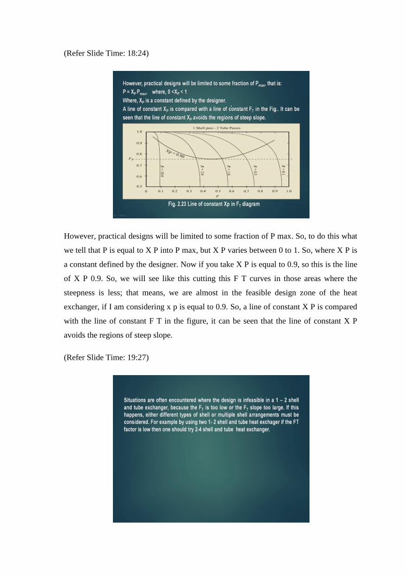
However, practical designs will be limited to some fraction of P max. So, to do this what

we tell that P is equal to X P into P max, but X P varies between 0 to 1. So, where X P is

a constant defined by the designer. Now if you take X P is equal to 0.9, so this is the line

of X P 0.9. So, we will see like this cutting this F T curves in those areas where the

steepness is less; that means, we are almost in the feasible design zone of the heat

exchanger, if I am considering x p is equal to 0.9. So, a line of constant X P is compared

with the line of constant F T in the figure, it can be seen that the line of constant X P

avoids the regions of steep slope.


Now situations are often encountered when the design is infeasible in a 1-2 shell and heat

exchanger, because the F T is too low, or the F T slopes are too high or too large or F T

slope is steep. If this happens, either different types of shell or multi shell arrangement

must be considered. For example, by using two 1-2 shell and tube heat exchanger the F T

factor is low then one should go for 2-4 shell and tube heat exchangers. Or if in one heat

exchanger, which is 1-2 shell and tube heat exchanger, the F T factor is low then I should

go for two shell and tube heat exchangers one to type seven tube exchangers to improve

the F T.


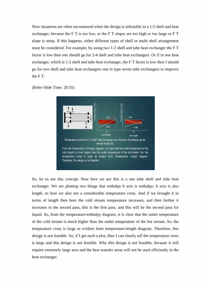
So, let us see this concept. Now here we see this is a one tube shell and tube heat

exchanger. We are plotting two things that enthalpy h axis is enthalpy; h axis is also

length, so here we also see a considerable temperature cross. And if we brought it in

terms of length then here the cold stream temperature increases, and then further it

increases in the second pass, this is the first pass, and this will be the second pass for

liquid. So, from the temperature-enthalpy diagram, it is clear that the outlet temperature

of the cold stream is much higher than the outlet temperature of the hot stream. So, the

temperature cross is large as evident form temperature-length diagram. Therefore, this

design is not feasible. So, if I get such a plot, then I can clearly tell the temperature cross

is large and this design is not feasible. Why this design is not feasible, because it will

require extremely large area and the heat transfer areas will not be used efficiently in the

heat exchanger.


So, my aim will be to improve the F T factor. So, the improvement can be done by

joining two one to seven tube heat exchangers in series. So, now, we consider two

numbers of shell and tube heat exchangers in series having enthalpy H 1 and H 2 such

that H 1 plus H 2 is H and this is H is our demanded H P enthalpy; that means, the load

for heat exchangers. This arrangement mimics a two shell pass and four tube pass heat

exchangers which is called 2-4 heat exchanger.

The temperature-enthalpy and temperature-length diagram for such a system is shown

below. So, if I see here, here I find no temperature cross, but here I find certain

temperature cross. Now if I analyze the shells here then I find that this temperature clot is

not large small temperature cross which can be accommodated. And here this shell does

not have the temperature cross. So, by increasing the number of shell passes, we can

distribute the temperature cross or we can decrease the temperature cross, and hence the

F T factor increases, and we move towards feasible design.


Now let us see a new concept, the concept of HRAT and EMAT, EMAT and HRAT.

This concept is based on a double temperature approach for the design of heat exchanger

network. The double temperature approach DTA requires the selection of two approach

temperature for synthesis of HEN. These temperatures are called the heat recovery

approach temperature – HRAT, and the exchanger minimum approach temperature –

EMAT. This approach differs from the work of Linnhoff and Flower as well as similar

works where authors have taken a single direct variable as delta T minimum. We have

seen that in most of the cases of heat integration, a single variable is taken and that is

delta T minimum. Here we see that two variables can be accommodated for this

purposes, and let us see what is the definition of HRAT and EMAT?


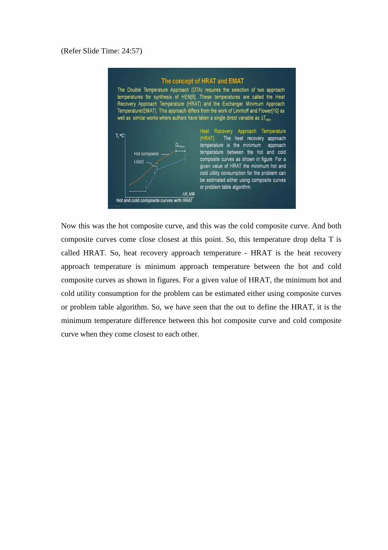
Now this was the hot composite curve, and this was the cold composite curve. And both

composite curves come close closest at this point. So, this temperature drop delta T is

called HRAT. So, heat recovery approach temperature - HRAT is the heat recovery

approach temperature is minimum approach temperature between the hot and cold

composite curves as shown in figures. For a given value of HRAT, the minimum hot and

cold utility consumption for the problem can be estimated either using composite curves

or problem table algorithm. So, we have seen that the out to define the HRAT, it is the

minimum temperature difference between this hot composite curve and cold composite

curve when they come closest to each other.


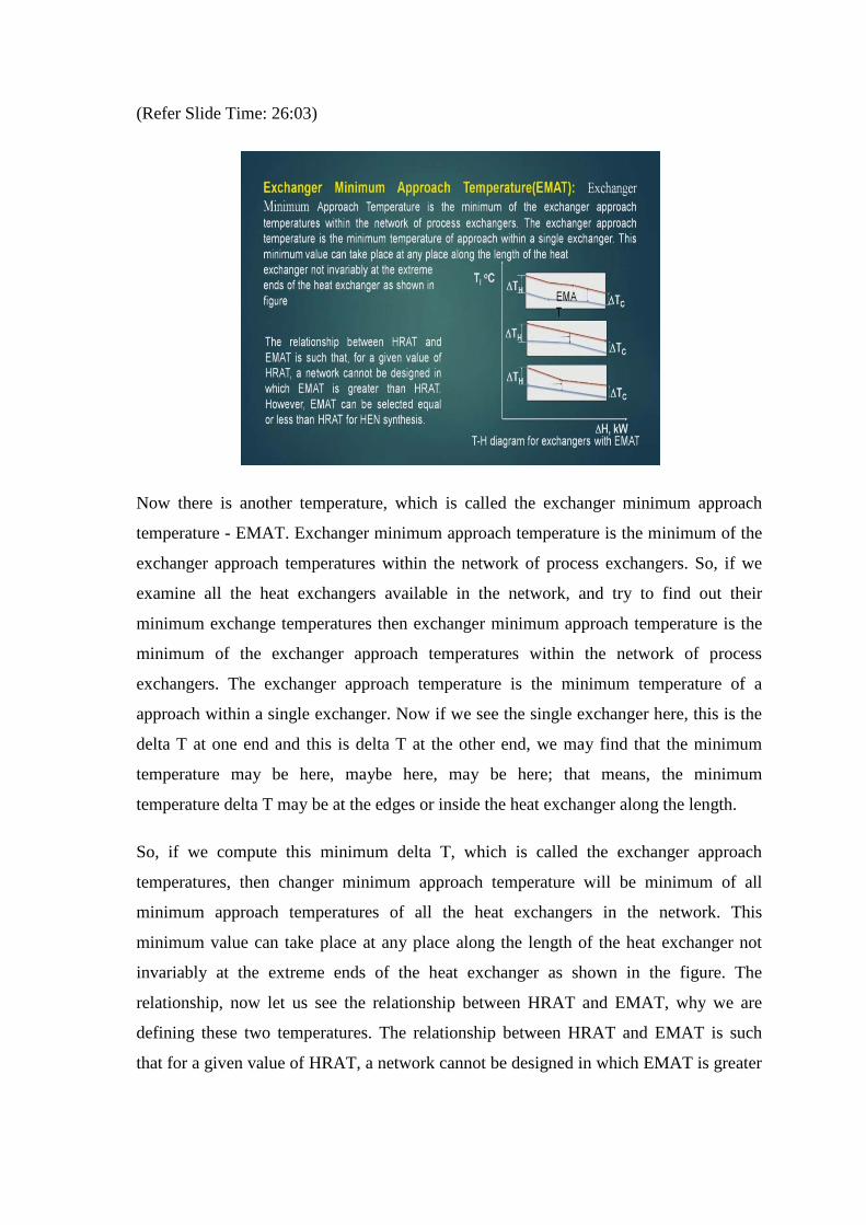
Now there is another temperature, which is called the exchanger minimum approach

temperature - EMAT. Exchanger minimum approach temperature is the minimum of the

exchanger approach temperatures within the network of process exchangers. So, if we

examine all the heat exchangers available in the network, and try to find out their

minimum exchange temperatures then exchanger minimum approach temperature is the

minimum of the exchanger approach temperatures within the network of process

exchangers. The exchanger approach temperature is the minimum temperature of a

approach within a single exchanger. Now if we see the single exchanger here, this is the

delta T at one end and this is delta T at the other end, we may find that the minimum

temperature may be here, maybe here, may be here; that means, the minimum

temperature delta T may be at the edges or inside the heat exchanger along the length.

So, if we compute this minimum delta T, which is called the exchanger approach

temperatures, then changer minimum approach temperature will be minimum of all

minimum approach temperatures of all the heat exchangers in the network. This

minimum value can take place at any place along the length of the heat exchanger not

invariably at the extreme ends of the heat exchanger as shown in the figure. The

relationship, now let us see the relationship between HRAT and EMAT, why we are

defining these two temperatures. The relationship between HRAT and EMAT is such

that for a given value of HRAT, a network cannot be designed in which EMAT is greater

than HRAT. So, this is the condition for the design of heat exchanger network. However,

EMAT can be selected equal or less than HRAT for HEN synthesis.


Now these are the references.

Thank you.

process integration prof. bikash mohanty department of...

Documents