Digitale filtreringsteknikker i anvendt geofysikk

Denne fremstillingen bygger på Eivind Ryggs forelesningshefte “Digitale filtreringsteknikker i anvendt geofysikk. (Universitetet i Bergen 1973). Og Costain and Coruh: Basic theory of exploration seismology. (2004)

1.1.Lowpass-filter

Et ideelt low pass filter slipper igjennom bare fourierkomponenter under en viss frekvens B. I frekvensdomenet vil derfor dette filterets utseende (amplituderespons) være en rektangulær kasse. Filtreringen skjer ved å multiplisere signalets fouriertransformasjon med denne rektangelfunksjonen. I følge konvolveringsteoremet tilsvarer en multiplikasjon i frekvensdomenet en konvolvering i tidsdomenet. Det betyr at hvis den filtreringen vi beskriver skulle utføres i tidsdomenet vil det måtte bli en konvolvering av signalet med filterets impulsrespons.Vi merker oss at filteret for eksempel F(f) i frekvensdomenet defineres dobbeltsidig og symmetrisk. Dersom F(f) bare ble definert mellom 0 og B ville dets avbilding i tidsdomenet, f(t), bli kompleks.

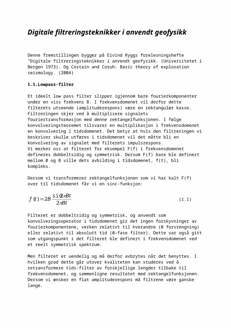
Dersom vi transformerer rektangelfunksjonen som vi har kalt F(f) over til tidsdomenet får vi en sinc-funksjon:

(1.1)

Filteret er dobbeltsidig og symmetrisk, og anvendt som konvolveringsoperator i tidsdomenet gir det ingen forskyvninger av fourierkomponentene, verken relativt til hverandre (0 forvrengning) eller relativt til absolutt tid (0-fase filter). Dette var også gitt som utgangspunkt i det filteret ble definert i frekvensdomenet ved et reelt symmetrisk spektrum.

Men filteret er uendelig og må derfor avbrytes når det benyttes. I hvilken grad dette går utover kvaliteten kan studeres ved å retransformere tids-filter av forskjellige lengder tilbake til frekvensdomenet, og sammenligne resultatet med rektangelfunksjonen. Dersom vi ønsker en flat amplituderespons må filtrene være ganske lange.

Det vil bli undulasjoner med maximum nær spekterets diskontinuitetspunkter, noe som skyldes at vi transfomerer avbrutte funksjoner. Dette kalles Gibbs-fenomener. Undulasjone har like store maksimalamplituder, og de øker i antall med økende filterlengde. For å få et bedre resultat må vi glatte F(f). En enkel måte å gjøre dette på er å veie filtrene.

Vi spør da: hva slags funksjon skal en bruke og i hvilket domene bør dette gjøres. Dette avhenger av hvor regnestykket blir enklest. Den operasjon som tilsvarer konvolvering i frekvensdomenet er i tidsdomenet multiplikasjon. Den glattingen vi har begrunnet i frekvensdomnet bør derfor utføres i tidsdomenet ved å multiplisere filteret med passende vekter.

Vi kan se kort på hva det vil si å se en tidsrekke gjennom et vindu. Fig.1 a. viser en sum av sinusoider med ulike frekvenser 1/T, 2/T,3/T der T er lengden av analyseringsvinduet. Disse frekvensene er harmoniske i forhold til hverandre og påvirker ikke hverandre.

15 10 5 5 10 15

1

1

2

3

Signal Plot

Fig.1.1.

Fouriertransformasjon til en sum av sinusoider vil være en rekke delta-funksjoner som er lokalisert nøyaktig på de korresponderende sinusoid-frekvenser uten noen interferens i et analyse-vindu av uendelig lengde. Men dersom vi velger bare et begrenset vindu å se signalet gjennom, må vi multiplisere sinusoidene med et rektangulært analyse vindu.

Matematisk kan vi skrive det slik:

F(w) = τ Sign (τ) (1+Sinc[2τw]) (1.2)

Der τ er bredden på analyse-vinduet. Da får vi energi lagt til undulasjoner i spekteret dersom vi har summen av flere sinusoider ( som 3/,2/T,1/T osv). Vi får energien på sinusoidenes frekvensspekter bevart når vi transformerer fra tid til frekvens, men vi får energi på ikke-harmoniske frekvenser som introduseres (for eksempel 2.4/T ). Når vi nå går tilbake ved å Fouriertransfomere spekteret vil vi få introdusert nye sinusoider som vil endre utseendet på trasen. Dette ser vi på fig.1.b. som viser tidsdomenet og fig.1.c som viser spekteret. Dette reiser et spørsmål om seismisk oppløsning, dvs. hvor lang må den trasen som vi studerer være for at vi skal ha nøyaktig prosessering av våre seismiske data.

15 10 5 5 10 15

2

1

1

2

3

4

Signal Plot

3 2 1 1 2 3 5

5

10

15

20

25

Sig nal Plot

Dersom vi ønsker en nærmere utgreiing av hva som har skjedd vil jeg gå litt mer i dybden på fig.2 der vi har de tre sinusoidene pluss en fjerde med frekvens 2.2/T :

Vi har benyttet et rektangulært vindu som kan presenteres i tid og frekvens øverst på figuren. Så kommer summen av sinusoidene. Og når vi legger denne til spekteret fjerde linje fra toppen på figuren, får vi den endelige trasen nederst.

15 10 5 5 10 15 2 1

1234

Signal Plot

3 2 1 1 2 3 5

510152025

Signal Plot

15 10 5 5 10 15 2 1

1234

Signal Plot

3 2 1 1 2 3

0.51

1.52

2.53

Sig nal Plot

15 10 5 5 10 15 1

1

2

3Signal Plot

3 2 1 1 2 3 5

5

10

15Signal Plot

15 10 5 5 10 15 1

1

2

3Signal Plot

3 2 1 1 2 3

0.51

1.52

2.53

Sig nal Plot

15 10 5 5 10 15

0.20.4

0.60.81

Sig nal Plot

3 2 1 1 2 3 5

51015202530

Signal Plot

Dersom vi bruker et vindu som er bredere enn det som er vist på fig.2. vil effekten av den tillagte frekvensen bli mindre. Og vi kan få den til å forsvinne helt ved å velge bredt nok vindu. Dette er illustrert på fig.1.3. der vi ser rektangelfunksjonen i tidsdomenet øverst, med de tilsvarende spektre under. Vi ser at spekteret nærmer seg mer og mer isolerte deltapulser.

20 10 10 20

0.2

0.4

0.6

0.8

1

Sig nal Plot

20 10 10 20

0.2

0.4

0.6

0.8

1

Sig nal Plot

20 10 10 20

0.2

0.4

0.6

0.8

1

Signal Plot

4 2 2 4 1

1

2

3

4

5

Signal Plot

4 2 2 4 2

2

4

6

8

10

Signal Plot

4 2 2 4 2.5

2.5

5

7.5

10

12.5

15

Signal Plot

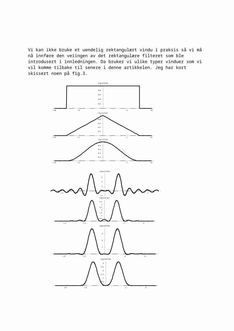
Vi kan ikke bruke et uendelig rektangulært vindu i praksis så vi må nå innføre den veiingen av det rektangulære filteret som ble introdusert i innledningen. Da bruker vi ulike typer vinduer som vi vil komme tilbake til senere i denne artikkelen. Jeg har kort skissert noen på fig.3.

10 5 5 10

0.2

0.4

0.6

0.8

1

Sig nal Plot

10 5 5 10

0.2

0.4

0.6

0.8

1

Signal Plot

10 5 5 10

0.2

0.4

0.6

0.8

1

Sig nal Plot

4 2 2 4

2

2

4

6

Signal Plot

4 2 2 4

0.5

1

1.5

2

2.5

3

3.5

Signal Plot

4 2 2 4

1

2

3

Sig nal Plot

4 2 2 4

0.5

1

1.5

2

2.5

3

Signal Plot

Fig.3. En rektangulær funksjon er veiet på ulike måter som gir et bedre spekter av sinusoidene fra Fig.1.

Generelt kan vi si at vinduet som er presentert på fig.1-2 vil være et lowpass-filter dersom vi ser på rektangelet i frekvensdomenet. Da vil lengden på rektangelet slik det er skissert bl.a. på toppen av fig.3. definere hvilke frekvenser som filteret slipper igjennom der diskontinuiteten definerer cut-off-frekvensen. Dermed er rektangelfunksjonens impulsrespons resultatet etter at filteret er anvendt på en seismisk input.

Da får vi en utvidelse ev utrykket (1.1):

(1.3)

Dette er imidlertid en kompleks tidsrekke, noe vi søker å unngå siden den skal brukes på reelle signaler. Det kan gjøres ved å definere filteret dobbeltsidig og symmetrisk i frekvensdomenet. Filterets styrke , dvs. dets totale arel må være som før, så vi fordeler arealet med like mye på hver side av symmetriaksen. Den tilsvarende impulsrespons vil være en sinc multiplisert med en cosinus-funksjon:

(1.4)

1.2. Andre filtertyper

High-pass filtrering anvendes når en ønsker å ta vare på et høyfrekevnt signal i lavfrekvent støy. Det kan enkelt lages ved å trekke et lavpassfilter fra et all-passfilter. (En all-pass operator har et flatt spektrum og slipper alle fourierkomponenter igjennom uattenuert.Et notch-filter er et filter som kutter et smalt frekvensbånd. Det kan være aktuelt å bruke når man vil fjerne lysnettstøy (50 Hz). Det kan også brukes til å fjerne en del av det seismiske signalet.

1.3. Filterkarakteristikker i dB og oktav

I det foregående har vi presentert filtrene i frekvensdomenet ved sine amplitudespektra som funksjon av frekvensen. Langs begge akser har vi brukt lineære skalaer. Mer vanlig er det å bruke logaritmisk skalering. Funksjonsaksen skaleres i decibel og frekvensaksen i oktav, og filterkarakteristikken blir gitt som decibel/oktav. (dB/oct).

Decibelskalaen er en logaritmisk skala med 10 som grunntall. Hvis A0 og A1 er amplituder er deres styrkeforhold utrykt i decibel:

(1.5)

Skalaen skal gi samme verdi i dB enten en bruker amplitudeforhold eller energi (effekt) forhold. Siden energien er proporsjonal med kvadratet av amplituden har vi:

E1 = k A12

E0 = k A02

E1/ E0 = A12/ A0

2 (1.6)

Oktav er en frekvensenhet og betyr fordobling av frekvensen fra et hvilket som helst utgangspunkt.

1.4.En annen innfallsvinkel

Komplekse tall kan også brukes til å beskrive enkle filteroperasjons som glatting og derivering. Dersom vi studerer en glattingsprosess som er vanlig å bruke på seismiske data har vi en utgangsrekke:

a0, a1, a2,….., an

Ut fra denne kan vi definere en toledds glatting ved utrykket:

(1.7)

Dersom vi antar at glattingskoeffisientene begge er like viktige, kan de representeres med fasere. Dersom

an= einw

vil output fra en toledds glatting bli

eller

(1.8)

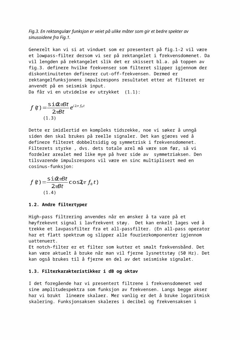
For å bestemme effekten av glatting må vi analysere leddet (1+eiw)/2 i (1.8) som er forholdet mellom output og input. Dersom vi bruker Eulers formel vil dette utrykket kunne skrives på formen:

cos(w/2)e-iw/2 (1.9)

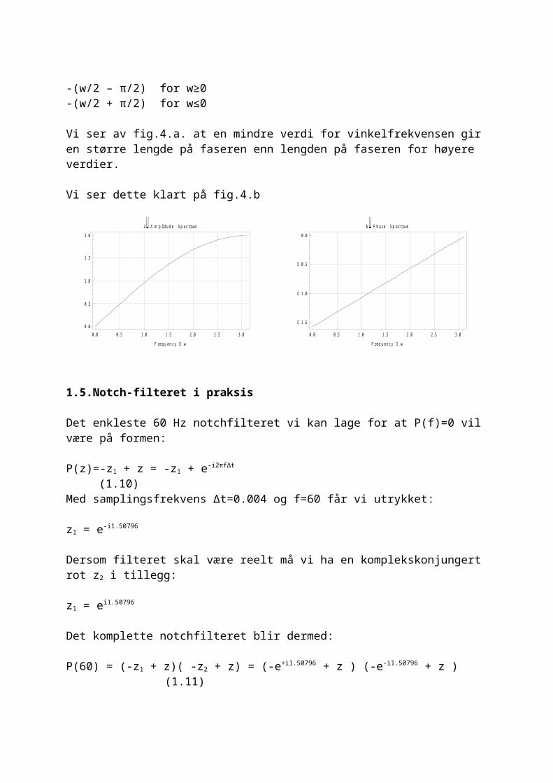
Og vi har fått et utrykk for en ny faser med modulen:

|cos(w/2)| og med en fase –w/2. Både modulen og fasen er funksjoner av vinkelfrekvensen som vises på fig. 4.a som et lowpass-filter:

0.0 0.5 1.0 1.5 2.0 2.5 3.00.0

0.2

0.4

0.6

0.8

1.0

F requency w

a A m p litude Sp ect rum

0.0 0.5 1.0 1.5 2.0 2.5 3.00.0

0.5

1.0

1.5

F requency w

b P hase Sp ect rum

Vi kan også studere derivering ved formelen:

bn=an+1 - an

Output av en toledds derivering vil bli bn=ei(n+1)w - einw

Eller:

bn= einw(eiw – 1)

for å forstå derivering vil vi måtte analysere leddet (eiw – 1) som kan utrykkes som en sinusfunksjon:

2 sin (w/2) ei(w/2 –π/2)

Der modulens spekter kan skrives:

|2 sin (w/2)| og representerer et high-pass filter. Fasespekteret er gitt ved:

-(w/2 – π/2)

Fase-spekteret skifter mellom –π/2 og π/2 og fasespekteret defineres derfor med utrykket:

-(w/2 – π/2) for w≥0-(w/2 + π/2) for w≤0

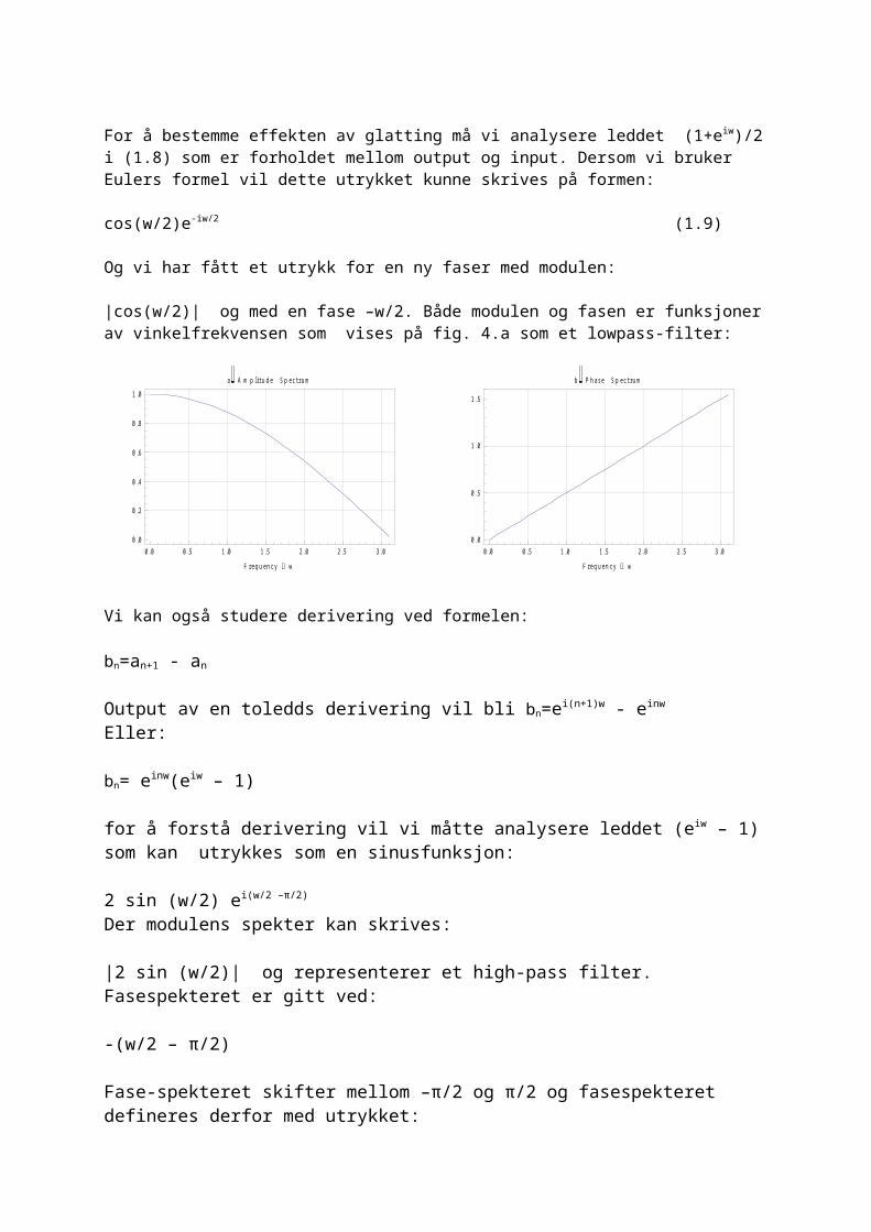
Vi ser av fig.4.a. at en mindre verdi for vinkelfrekvensen gir en større lengde på faseren enn lengden på faseren for høyere verdier.

Vi ser dette klart på fig.4.b

0.0 0.5 1.0 1.5 2.0 2.5 3.00.0

0.5

1.0

1.5

2.0

F requency w

a A mp litude Sp ect rum

0.0 0.5 1.0 1.5 2.0 2.5 3.0

1.5

1.0

0.5

0.0

F requency w

b P hase Sp ect rum

1.5.Notch-filteret i praksis

Det enkleste 60 Hz notchfilteret vi kan lage for at P(f)=0 vil være på formen:

P(z)=-z1 + z = -z1 + e-i2πf∆t (1.10)Med samplingsfrekvens ∆t=0.004 og f=60 får vi utrykket:

z1 = e-i1.50796

Dersom filteret skal være reelt må vi ha en komplekskonjungert rot z2 i tillegg:

z1 = ei1.50796

Det komplette notchfilteret blir dermed:

P(60) = (-z1 + z)( -z2 + z) = (-e+i1.50796 + z ) (-e-i1.50796 + z ) (1.11)

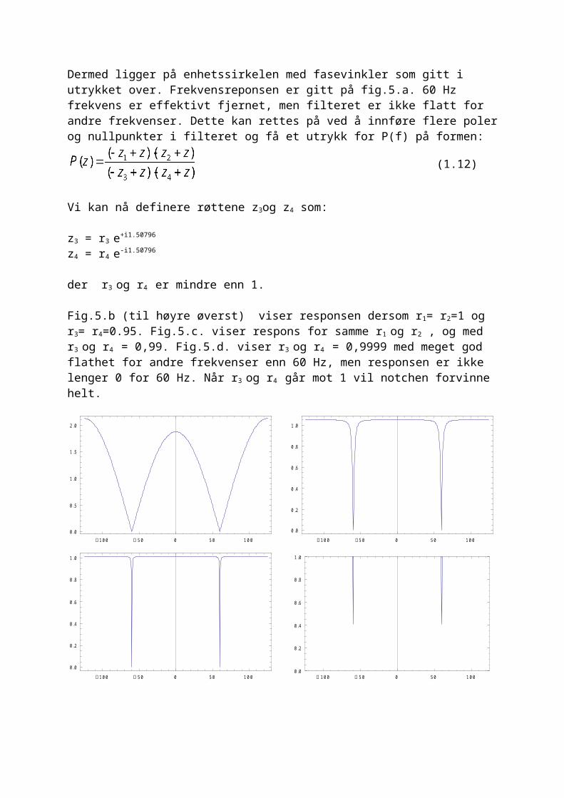
Dermed ligger på enhetssirkelen med fasevinkler som gitt i utrykket over. Frekvensreponsen er gitt på fig.5.a. 60 Hz frekvens er effektivt fjernet, men filteret er ikke flatt for andre frekvenser. Dette kan rettes på ved å innføre flere poler og nullpunkter i filteret og få et utrykk for P(f) på formen:

(1.12)

Vi kan nå definere røttene z3og z4 som:

z3 = r3 e+i1.50796

z4 = r4 e-i1.50796

der r3 og r4 er mindre enn 1.

Fig.5.b (til høyre øverst) viser responsen dersom r1= r2=1 og r3= r4=0.95. Fig.5.c. viser respons for samme r1 og r2 , og med r3 og r4 = 0,99. Fig.5.d. viser r3 og r4 = 0,9999 med meget god flathet for andre frekvenser enn 60 Hz, men responsen er ikke lenger 0 for 60 Hz. Når r3

og r4 går mot 1 vil notchen forvinne helt.

10 0 50 0 50 10 00 .0

0 .5

1 .0

1 .5

2 .0

10 0 50 0 50 10 0

0 .0

0 .2

0 .4

0 .6

0 .8

1 .0

10 0 50 0 50 10 0

0 .0

0 .2

0 .4

0 .6

0 .8

1 .0

10 0 50 0 50 10 00 .0

0 .2

0 .4

0 .6

0 .8

1 .0

2.0 Digital Filter Design Techniques

2.0 Introduction

This outline is build on chapter 5 in Oppenheim and Schafers book: Digital Signal processing: In the most general sense, a digital filter is a linear shift-invariant discrete-time system that is realized using finite-precision arithmetic. The design of digital niters involves three basic steps: (1) the specification of the desired properties of the system; (2) the approximation of these specifications using a causal discrete-time system; and (3) the realization of the system using finite-precision arithmetic. Although these three steps are certainly not independent, I will focus attention in this article primarily on the second step, the first being highly dependent on the application, and the third being discussed in another article.

In a practical setting, it is often the case that the desired digital filter is to be used to filter a digital signal that is derived from an analog signal by means of periodic sampling. The specifications for both analog and digital filters are often (but not always) given in the frequency domain, as, for example, in the case of frequency selective filters such as lowpass, bandpass, and high-pass filters. Given the sampling rate, it is straightforward to convert from frequency specifications on an analog filter to frequency specifications on the corresponding digital filter, the analog frequencies being in terms of Hertz and the digital frequencies being in terms of radian frequency or angle around the unit circle with the point z = - 1 corresponding to half the sampHng frequency. There are, however, applications in which a digital signal to be filtered is not derived by means of periodic sampling of an analog time function, and there are a variety means besides periodic sampling for representing analog time functions in terms of sequences. Furthermore, in most of the design techniques that we shall discuss, the sampling period plays no role whatsoever in the approximation procedure.

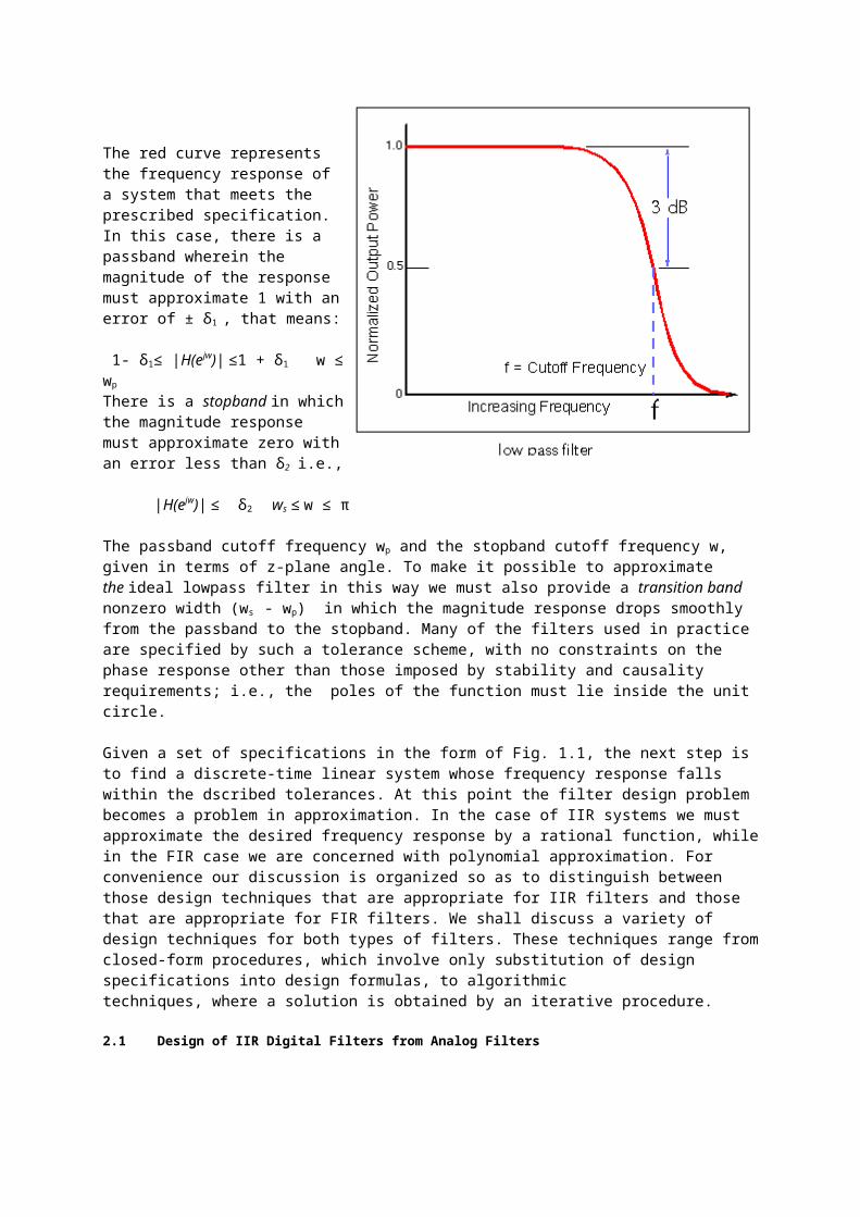
Therefore, the least confusing point of view toward digital filter design is to consider the filter as being specified in terms of angle around the unit circle rather than in terms of analog frequencies.A separate problem is that of determining an appropriate set of specifications on the digital filter. In the case of a lowpass filter, for example, the specifications often take the form of a tolerance scheme, such as depicted in Fig. 2.l. (right side below)

The red curve represents the frequency response of a system that meets the prescribed specification. In this case, there is a passband wherein the magnitude of the response must approximate 1 with an error of ± δ1 , that means:

1- δ1≤ |H(ejw)| ≤1 + δ1 w ≤ wp

There is a stopband in which the magnitude response must approximate zero with an error less than δ2 i.e.,

|H(ejw)| ≤ δ2 ws ≤ w ≤ πThe passband cutoff frequency wp and the stopband cutoff frequency w, given in terms of z-plane angle. To make it possible to approximate the ideal lowpass filter in this way we must also provide a transition band nonzero width (ws - wp) in which the magnitude response drops smoothly from the passband to the stopband. Many of the filters used in practice are specified by such a tolerance scheme, with no constraints on the phase response other than those imposed by stability and causality requirements; i.e., the poles of the function must lie inside the unit circle.

Given a set of specifications in the form of Fig. 1.1, the next step is to find a discrete-time linear system whose frequency response falls within the dscribed tolerances. At this point the filter design problem becomes a problem in approximation. In the case of IIR systems we must approximate the desired frequency response by a rational function, while in the FIR case we are concerned with polynomial approximation. For convenience our discussion is organized so as to distinguish between those design techniques that are appropriate for IIR filters and those that are appropriate for FIR filters. We shall discuss a variety of design techniques for both types of filters. These techniques range from closed-form procedures, which involve only substitution of design specifications into design formulas, to algorithmictechniques, where a solution is obtained by an iterative procedure.

2.1 Design of IIR Digital Filters from Analog Filters

The traditional approach to the design of IIR digital filters involves the transformation of an analog filter into a digital filter meeting prescribed specifications. This is a reasonable approach because:

1. The art of analog filter design is highly advanced and, since useful results can be achieved, it is advantageous to utilize the design procedures already developed for analog filters.

2. Many useful analog design methods have relatively simple closed-form design formulas. Therefore, digital filter design methods based on such analog design formulas are rather simple to implement.

3. In many applications it is of interest to use a digital filter to simulate the performance of an analog linear time-invariant filter.

Consider an analog system function,

(2.1)

Where xa(t) is the input and ya(t) is the output and Xa(s) and Ya(s) are their respective Laplace transforms. It is assumed that Ha(s) has been obtained through one of the established approximation methods used in analog filter design.

The input and output of such system are related by the convolution integral,

(2.2)

where ha(t), the impulse response, is the inverse Laplace, transform of Ha(s). Alternatively, an analog system having a system function Ha(s) can described by the differential equation

The corresponding rational system function for digital filters has the form

The input and output are related by the convolution sum

(2.5)

or, equivalently, by the difference equation

In transforming an analog system to a digital system we must therefore obtain either H(z) or h(n) from the analog filter design. In such transformations we generally require that the essential properties of the analog frequency response be preserved in the frequency response of the resulting digital filter. Loosely speaking, this implies that we want the imaginary axis of the s-plane to map into the unit circle of the z-plane. A second condition is that a stable analog filter should be transformed to a stable digital filter. That is, if the analog system has poles only in the left-half 5-plane, then the digital filter must have poles only inside the unit circle. These constraints are basic to all the techniques to be discussed in this section.

2.1.1 Impulse Invariance

One procedure for transforming an analog filter design to a digital filter design corresponds to choosing the unit-sample response of the digital filter as equally spaced samples of the impulse response of the analog filter, That is,

h(n) = ha(nT)

where T is the sampling period.

It can be shown as a generalization that the z-transform of h(n) is related to the Laplace transform of ha(t) by the equation

(2.7)

From the relationship z = esT it is seen that strips of width 2π/T in the s-plane map into the entire z-plane as depicted in Fig. 1.2. The left half of each s-plane strip maps into the interior of the unit circle, the right half of each s-plane strip maps into the exterior of the unit circle, and the imaginary axis of the s-plane maps onto the unit circle in such a way that each segment of length 2π/T is mapped once around the unit circle.

From Eq. (1.7) it is clear that each horizontal strip of the s-plane is overlayed onto the z-plane to form the digital system function from the analog system function. Thus the impulse invariance method does not correspond to a simple algebraic mapping of the s-plane to the z-plane.

The frequency response of the digital filter is related to the frequency response of the analog filter as

(2.8)

From the sampling theorem it is clear that if and only if

Ha (jω) = 0, |ω| > π/T ,

Unfortunately, any practical analog filter will not be bandlimited, and consequently there is interference between successive terms in Eq. (1.8) as illustrated in Fig. 1.3.

Because of the aliasing that occurs in the sampling process, the frequency response of the resulting digital filter will not be identical to the original analog frequency response. It is important to note that if we consider the filter specifications to be in terms of specifications on a digital filter, then a change in the value of T has no effect on the amount of aliasing in the impulse invariant design procedure. For example, referring to Fig. 1.3, we may consider that the cutoff frequency of the digital filter has been specified to be at the frequency labeled ωaT. That point in the frequency response is then constrained as the cutoff frequency of a lowpass digital filter, and if T is reduced, then ωa in the analog filter must be correspondingly increased in such a way that ωaT remains constant and equal to the cutoff frequency specified for the digital filter. Thus if T is made smaller in an effort to reduce the effect of aliasing, ωa must be made correspondingly larger. With the attitude that the digital filter to be designed is specified in terms of frequencies on the unit circle, T is therefore an irrelevant parameter in impulse invariant design and could just as well be considered to be equal to unity. While it is common practice to include the parameter T in discussing impulse invariant design, it is important to keep in mind that the parameter plays a minor role in the design procedure.

To investigate the interpretation of impulse invariant design in terms of a relationship between the s-plane and the z-plane, let us consider the system function of the analog filter expressed in terms of a partial-fraction expansion, so that

(2.9)

The corresponding impulse response is

where u(t) is a continuous-time unit step function. And the unit-sample response of the digital filter is then

The system function of the digital filter H(z) is consequently given by

(2.10)

In comparing Eqs. (1.9) and (1.10) we observe that a pole at s = sk in the s-plane transforms to a pole at eskT

in the z-plane and the coefficients in the partial-fraction expansion of Ha(s) and H(z) are equal. If the analog filter is stable, corresponding to the real part of sk less than zero, then the magnitude of eSkT will be less than unity, so that the corresponding pole in the digital filter is inside the unit circle, and consequently the digital filter is also stable. While the poles in the s-plane map to poles in the z-plane according to the relationship zk = eskT , it is important to recognize that the impulse invariant design procedure does not correspond to a mapping of the s-plane to the z-plane by that relationship or in fact by any relationship. In particular, the zeros of the digital transfer function are a function of the poles and the coefficients Ak in the partial-fraction expansion and they will not in general be mapped in the same way the poles are mapped.It should be noted that when the analog filter is "sufficiently bandlimited” the above procedure produces a digital filter whose frequency respons from Eq. (1.8),

Thus, for high sampling rates (Tsmall) the digital filter may have an extremely high gain. For this reason it is generally advisable to use, instead of Eq.(1.10),

(2.11)

That is, the unit-sample response is h(n) = Tha(nT).

The basis for impulse invariance as described above is to choose a unit-sample response for the digital filter that is similar in some sense to the impulse response of the analog filter. The use of this procedure is often not motivated so much by a desire to maintain the impulse response shape, but by the knowledge that if the analog filter is bandlimited, then the digital filter frequency response will closely approximate the analog frequency response. However, in some filter design problems, a primary objective may be to control some aspect of the time response such as the impulse response or the step response. In such cases a natural approach would be to design the digital filter by impulse invariance or a step invariance procedure. In the latter case, the response of the digital filter to a sampled unit step function is chosen to be samples of the analog step response. In this way, if the analog filter has good step response characteristics, such as small rise time and low peak overshoot, these characteristics would be preserved in the digital filter. Clearly, this concept of waveform invariance can be extended to the preservation of the output waveshape for a variety of inputs.

Although in the impulse invariance design procedure, distortion in the frequency response is introduced due to aliasing, the relationship between analog and digital frequency is linear and consequently, except for aliasing, the shape of the frequency response is preserved. This is in contrast to the procedures to be discussed next, which correspond to the use of algebraic transformations. It should be noted in conclusion that the impulse invariance technique is obviously only appropriate for essentially bandlimited filters. For example, highpass or bandstop filters would require additional band-'irniting to avoid severe aliasing distortion.

2.1.2 Designs Based on Numerical Solution of the Differential Equation

A second approach to deriving a digital filter is to approximate the derivatives in Eq. (1.3) by finite differences. This is a standard procedure in numerical analysis and in digital simulations of analog systems. This procedure can be motivated by the intuitive notion that the derivative of an analog time function can be approximated by the difference between consecutive samples of the function to be differentiated. We might expect that the sampling rate is increased, i.e., the samples are closer together, then the approximation to the derivative would be increasingly accurate. For example, suppose that the first derivative is approximated by the first back ward difference

where y(n) = ya(nT). Approximations to higher-order derivatives are obtained by repeated application of Eq. (5.12

This can be solved applying finite difference method outlined on page 205 in Oppenheim and Schafer

which corresponds to a circle whose center is at z = J and radius is \ as shown in Fig. 5.5. It is easily verified that the left half of the j-plane maps the inside of the small circle and the right half of the s-plane maps into outside of the circle. Therefore, although the requirement of mapping the axis to the unit circle is not satisfied, this mapping does satisfy the sta-'ty condition since poles in the left half j-plane map to the inside of the circle, which is inside the unit circle.

It is worth correlating this result with a common intuitive notion. It is generally assumed that the simulation on a digital computer of the processing of a continuous-time signal by a differential equation can be accomplished by replacing derivatives by differences if the continuous signal is sampled at a high-enough rate. For example, if we wish to differentiate a continuous signal we intuitively expect that an approximation to the deriva tive can be accomplished by sampling the continuous-time function with a small-enough spacing between samples and forming the first difference of the resulting sequence. To show that in fact this intuition is consistent with the results that we just obtained, we remark first of all that if a bandlirnited analog signal is sampled at the Nyquist rate, then the spectrum is nonzero over the entire unit circle. As we increase the sampling rate from the Nyquist rate, that is, as we decrease the sampling period, the nonzero part of the spectrum of the digital signal is confined to a smaller and smaller portion of the unit circle, and, in particular, if we choose the sampling period to be sufficiently small, we can concentrate the nonzero part of the spectrum in the vicinity of z = 1 in the z-plane. Correspondingly, if T is sufficiently small in Eq. (5. 1 3), then the frequency response of the digital filter will be concentrated on the small circle in Fig. 5.5 in the vicinity of z = 1. This is, of course, the point at which the small circle and the unit circle are tangent, and if both the filter response and the signal spectrum are concentrated in that region, then we can expect that the digital filter will accurately approximate the analog filter.

In the above procedure, derivatives were replaced by backward differences. An alternative approximation to the derivative is a forward difference. The first forward difference is defined asThe mapping corresponding to this approximation is examined in Problem 2 of this chapter, where it is shown that unstable digital filters can result from this approximation.

The major point in the previous example and also in Problem 2 of this chapter is that, in contrast to the impulse invariance technique, decreasing the sampling period theoretically produces a better filter since the spectrum tends to be concentrated in a very small region of the unit circle. In general, however, there is little to recommend the use of forward or backward differences in digital signal processing, since the high sampling rates required result in a very inefficient representation of the filter and the input signal. Furthermore, it is clear that these procedures are highly unsatisfactory for anything but lowpass filters. Thus we are led to consider other mappings that avoid the aliasing problems of the impulse invariance method.

Examples: Analog-Digital Transformation

The techniques of the previous section rely upon the availability of appropriate analog filter designs. In this section we discuss examples of several analog lowpass approximation techniques, including Butterworth, Chebyshevs, and elliptic approximations. The discussion is organized as follows: first, we present the basic design formulas for a particular approximation method. Then, using the same lowpass filter specifications for each approximation method, we carry out the design of a digital filter using both impulse invariance and bilinear transformation .

2.2.1 Digital Butterworth Filters

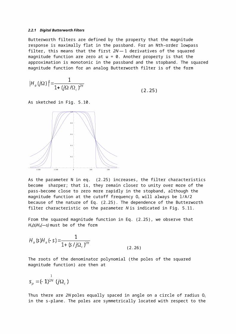
Butterworth filters are defined by the property that the magnitude response is maximally flat in the passband. For an Nth-order lowpass filter, this means that the first 2N — 1 derivatives of the squared magnitude function are zero at ω = 0. Another property is that the approximation is monotonic in the passband and the stopband. The squared magnitude function for an analog Butterworth filter is of the form

(2.25)

As sketched in Fig. 5.10.

20 0 10 0 0 10 0 20 0

0 .2

0 .4

0 .6

0 .8

1 .0

As the parameter N in eq. (2.25) increases, the filter characteristics become sharper; that is, they remain closer to unity over more of the pass-become close to zero more rapidly in the stopband, although the magnitude function at the cutoff frequency Oc will always be l/A/2 because of the nature of Eq. (2.25). The dependence of the Butterworth filter characteristic on the parameter N is indicated in Fig. 5.11.

From the squared magnitude function in Eq. (2.25), we observe that Ha(s)Ha(—s) must be of the form

(2.26)

The roots of the denominator polynomial (the poles of the squared magnitude function) are then at

Thus there are 2N poles equally spaced in angle on a circle of radius Oc in the s-plane. The poles are symmetrically located with respect to the imaginary axis. A pole never falls on the imaginary axis and one occurs"on the real axis for N odd but not for N even. The angular spacing between the poles on the circle is Π/N radians. For example, for N = 3, the poles are spaced by w/3 radians or by 60 degrees, as indicated in Fig. 5.12. To determine the transfer function of the analog filter to associate with the Butterworth squared magnitude function, we wish to perform the factorization Ha(s)Ha(—s). We observe that the poles of the Butterworth squared magnitude function occur in pairs, so that if there is a pole at s = sp, then a pole also occurs at s = —sp . Consequently, to construct Ha(s) from the squared magnitude function, we would choose one pole from each such pair. If we restrict the filter to be stable and causal, which is generally the case, then these poles will correspond to the poles on the left-half-plane part of the Butterworth circle. If we obtain a digital Butterworth filter from an analog Butterworth filter by mapping the pole pattern from the s-plane to the z-plane using the bilinear transformation, then in the z-plane the corresponding squared magnitude function has2N zeros at z = — 1.

The Butterworth circle in the s-plane then maps to a circle in the z-plane, since the bilinear transformation is a conformal mapping. However, the Butterworth circle in the z-plane is not centered at the origin. This circle in the z-plane is indicated in Fig. 2.2.

While the poles in the s-plane were equally spaced in angle on the Butterworth circle, that is no longer true in the z-plane. In fact, pole pairs at sp and —s.,, in the s-plane map to pole pairs at zp and l/zp in the z-plane.

Generally, in designing a Butterworth filter using the bilinear transformation, the most straightforward procedure is to first determine the location of the poles in the s-plane and then map the left-hand plane poles to the z-plane with the appropriate transformation, rather than attempt to locate the poles directly in the z-plane.

3.1 Design of FIR Filters Using Windows

The most straightforward approach to FIR filter design is to obtain a finite-length impulse response by truncating an infinite-duration impulse response sequence. If we suppose that Hd(eiw) is an ideal desired frequency response, then

(3.49a)

where hd(n) is the corresponding impulse response sequence, i.e.,

(5.49b)

In general, Hd (ejw ) for a frequency selective filter may be piecewise constant with discontinuities at the boundaries between bands. In such cases the sequence hd(n) is of infinite duration and it must be truncated to obtain a finite-duration impulse response. As we have pointed out before, Eqs. (5.49) can be thought of as a Fourier series representation of the periodic frequency response Hd(eiw), with the sequence hd(n) playing the role of the "Fourier coefficients." Thus the approximation of an ideal filter specification by truncation of the ideal impulse response is identical to the study of the convergence of Fourier series, a subject that has received a great deal of study since the middle of the eighteenth century. The most familiar concept from this theory is the Gibbs phenomenon. In the following discussion we shall see how this nonuniform convergence phenomenon manifests itself in the design of FIR filters.

If hd(n) has infinite duration, one way to obtain a finite-duration causal impulse response is to simply truncate h(n), i.e., define

In general, we can represent h(n) as the product of the desired impulsresponse and a finiteduration "window" w(n); i.e.,

h(n) = hd (n) w(n)

where in the example

(5.52)

Using the complex convolution theorem see that

(5.53)

That is, H(eiw) is the periodic continuous convolution of the desired frequency response with the Fourier transform of the window. Thus the frequency response H(ejw) will be a "smeared" version of the desired response Hd(ejw).

Figure 5.31 (a) depicts typical functions Hd(eiθ) and W(eiw-θ) required in Eq. (5.53). (Both are shown as real

functions only for convenience in depicting the convolution process.)

From Eq. (5.53) we see that if W(eiw) is narrow compared to variations in Hd(eim), then H(ejm) will "look like" Hd(ei<a). Thus the choice: of.window is_gpverned by the desire to have vr(«) as short as, possible in duration so as to minimize computation in the implementation of the filter, while having W(e}m) as narrow as possible in frequency so as to faithfully reproduce the desired frequency response. These are conflicting requirements, as can be seen in the case of the rectangular window of Eq. (5.52), where

The magnitude of W(e'm) is sketched in Fig. 5.32 for N = 8 and the phase is linear, as can be seen from Eq. (5.54). As N increases, the width of the "main lobe" decreases. (The main lobe is arbitrarily defined as the region between w = -2π/N and +2n/N.)

However, for the rectangular window, the "side lobes" are not insignificant and, in fact, as N increases, the peak amplitudes of the main lobe and the side lobes grow in a manner such that the area under each lobe is a constant, while the width of each lobe decreases with N. The result of this is that as W(ej(w-θ)) slides by a discontinuity of Hd(eie) with increasing w, the integral of W(ej(w-θ))Hd (ejθ ) will vary in an oscillatory manner as each lobe of W(ej(w-θ))) moves past the discontinuity. This is depicted in Fig. 5.31 (b). Since the area under each lobe remains constant with increasing N, the oscillations only occur more rapidly but do not decrease in amplitude as N increases. In the theory of Fourier series, it is well known that this non-uniform convergence, the Gibbs phenomenon, can be moderated through the use of a less abrupt truncation of the Fourier series.

By tapering the window smoothly to zero at each end, the height of the side lobes can be diminished; however, this is achieved at the expense of a wider main lobe and thus a wider transition at the discontinuity. Examples °f some commonly used windows are shown in Fig. 5.33. These windows are specified by the following equations [21]:

Rectangular:

W(n)=1 0≤ n ≤ N-1

Bartlett:

Hanning:

0 ≤ n ≤ N-1

Hamming:

0 ≤ n ≤ N-1

Blackman:

(5.55e)

The function 20 log10 |W(eiw)| is plotted in Fig. 5.34 for each of these windows for N = 51. Note that since these windows are all symmetrical, the phase is linear. The rectangular window clearly has the narrowest main lobe and thus, for a given length, jV should yield the sharpest transitions of H(ei<0) at a discontinuity of Hd(ejm). However, the first side lobe is only about 13 dB below the main peak, resulting in oscillations of H(e}<0) Ol considerable size at a discontinuity of Hd(e]m). By tapering the window smoothly to zero, the side lobes are greatly reduced; however, it is de* that the price paid is a much wider main lobe and thus wider transitions a discontinuities of Hd(ei<a).

Kaiser [4] has proposed a flexible family of windows defined by

where I0( ) is the modified zeroth order Bessel function of the first kind. Kaiser has shown that these windows are nearly optimum in the sense of having the largest energy in the main lobe for a given peak side lobe amplitude. The parameter wa can be adjusted so as to trade off main-lobe width for side-lobe amplitude. Typical values of wa((N — l)/2) are in the range

4<wa((N-1)/2) <9

0 .4 0 .2 0 .0 0 .2 0 .4 80

60

40

20

0

20

40

no rmalized freq uency

ampl

itude

dB

Rectangular (Dirichlet) window

0 .4 0 .2 0 .0 0 .2 0 .480

60

40

20

0

20

40

no rmalized frequency

ampl

itude

dB

Rectangular (Bartlett) window

0 .4 0 .2 0 .0 0 .2 0 .480

60

40

20

0

20

40

no rmalized frequency

ampl

itude

dB

Hanning window

0 .4 0 .2 0 .0 0 .2 0 .480

60

40

20

0

20

40

no rmalized frequency

ampl

itude

dB

Hamming window

0 .4 0 .2 0 .0 0 .2 0 .4 80

60

40

20

0

20

40

no rmalized freq uency

ampl

itude

dB

Blackman window

As an illustration of the use of windows in filter design, consider the design of a lowpass filter. Anticipating the need for delay in achieving a causal linear-phase filter, the desired frequency response is defined as

The corresponding impulse response is

Clearly, hd(n) has infinite duration. To create a finite-duration linear-phase causal filter of length N, we defineh(n) = ha(n)w(n) where

α =( N-1)/2

It can easily be verified that if w(n) is symmetrical, this choice of a results in a sequence h(n) satisfying Eq. (5.47). Figure 5.35 shows a plot of hd(ri) for a rectangular window, N =51, and eoc = 77/2. Figure 5.36 shows 201og10 I#(e30))| for the impulse response of Fig. 5.35 weighted by each of five windows of Fig. 5.34. Note the increasing transition width, corresponding to increasing main-lobe width, and the increasing stopband attenuation, corresponding to decreasing side-lobe amplitude. From Eq. (5.54) we note that the width of the central lobe is inversely proportional to N. This is generally true and is illustrated for a Hamming window in Fig. 5.37, where it is clearly evident that as N is doubled, the width of the central lobe is halved. Figure 5.38 illustrates the effect of greasing N on the transition region in a lowpass filter design. Clearly, the minimum stopband attenuation remains essentially constant, being dependent on the shape of the window, while the width of the transition region at the discontinuity of Ha(eia>) depends on the length of the window.

The examples that we have given illustrate the general principles of the windowing method of FIR filter design. Through the choice of the window ape and duration, we can exercise some control over the design process.

For example, for a given stopband attenuation, it is generally true that N satisfies an equation of the form

N= (A/∆w)

where ∆w is the transition width [roughly the width of the main lobe of W(e1<a)] and A is a constant that is dependent upon the window shape. As we have seen, the window shape is essential in determining the minimum stopband attenuation. For the windows that we have discussed, the basic Parameters for lowpass filter design are summarized in Table 5.2. It should °e noted that the values in Table 5.2 are approximate; they depend somewhat uP°n N and the cutoff frequency of the desired filter. Kaiser's windows, kq- (5.55e), have a variable parameter, coa, whose choice controls the tradeoff between side-lobe amplitude and side-lobe width. Tables and curves §°verning the use of these windows are given by Kaiser [4,22].

Impulse response Hamming window

0 .4 0 .2 0 .0 0 .2 0 .480

60

40

20

0

20

40

normalized frequency

amp

litu

dedB

Time index=25 n=11 Hamming window

0 .4 0 .2 0 .0 0 .2 0 .4 80

60

40

20

0

20

40

no rmalized freq uency

amp

litu

dedB

Time index=51 n=11 Hamming window

0 .4 0 .2 0 .0 0 .2 0 .4 80

60

40

20

0

20

40

no rmalized freq uency

amp

litu

dedB

Time index=101 n=11 Hamming window

The basic principles illustrated by our examples are true in general and j;atl be applied in the design of any filter for which we can define a desired ^equency response. In this sense, the technique has considerable generality.

However, a difficulty with the technique is in the evaluation of the integral ln Eq. (5.49b). If Ha(eim) cannot be expressed in terms of simple functions for which the integration can be performed, an approximation to hd(n) must be obtained by sampling Hd(e'm) and using the inverse discrete Fourier transform to compute

If M is large, hd(n) can be expected to be a good approximation to hd(ri) in the interval of the window. Another limitation of the procedure is that it is somewhat difficult to determine, in advance, the type of window and the duration N required to meet a given prescribed frequency response specifica-tion.f However, a very simple digital computer program can be used to make such a determination by a trial-and-error procedure. Thus, design of digital filters using a window is often a convenient and satisfactory approach.

Design of windows using Audacity

It is a good idea to train on windowing technics with a good developing software. A program well suited for that is the free program Audacity for sound editing. It is developed from Sourceforge and under a free liscence. We will do some application with Audacity to illustrate our theory.An interesting aspect with Audacity is that you can hear the sequence you train on as sound, when you develop.