digital filter structures and quantization error analysis1.1... · digital filter structures and...

Digital Filter Structures and QuantizationError Analysis

By:Douglas L. Jones

Digital Filter Structures and QuantizationError Analysis

By:Douglas L. Jones

Online:< http://cnx.org/content/col10259/1.1/ >

C O N N E X I O N S

Rice University, Houston, Texas

This selection and arrangement of content as a collection is copyrighted by Douglas L. Jones. It is licensed under the

Creative Commons Attribution 1.0 license (http://creativecommons.org/licenses/by/1.0).

Collection structure revised: January 2, 2005

PDF generated: October 25, 2012

For copyright and attribution information for the modules contained in this collection, see p. 41.

Table of Contents

1 Filter Structures1.1 Filter Structures . . . . . . . . . . . . . . . . . . . . . . . . . . . . . . . . . . . . . . . . . . . . . . . . . . . . . . . . . . . . . . . . . . . . . . . . . . . . . 11.2 FIR Filter Structures . . . . . . . . . . . . . . . . . . . . . . . . . . . . . . . . . . . . . . . . . . . . . . . . . . . . . . . . . . . . . . . . . . . . . . . . 11.3 IIR Filter Structures . . . . . . . . . . . . . . . . . . . . . . . . . . . . . . . . . . . . . . . . . . . . . . . . . . . . . . . . . . . . . . . . . . . . . . . . 51.4 State-Variable Representation of Discrete-Time Systems . . . . . . . . . . . . . . . . . . . . . . . . . . . . . . . . . . . . 11

2 Fixed-Point Numbers2.1 Fixed-Point Number Representation . . . . . . . . . . . . . . . . . . . . . . . . . . . . . . . . . . . . . . . . . . . . . . . . . . . . . . . . 152.2 Fixed-Point Quantization . . . . . . . . . . . . . . . . . . . . . . . . . . . . . . . . . . . . . . . . . . . . . . . . . . . . . . . . . . . . . . . . . . . 17

3 Quantization Error Analysis

3.1 Finite-Precision Error Analysis . . . . . . . . . . . . . . . . . . . . . . . . . . . . . . . . . . . . . . . . . . . . . . . . . . . . . . . . . . . . . 193.2 Input Quantization Noise Analysis . . . . . . . . . . . . . . . . . . . . . . . . . . . . . . . . . . . . . . . . . . . . . . . . . . . . . . . . . . 213.3 Quantization Error in FIR Filters . . . . . . . . . . . . . . . . . . . . . . . . . . . . . . . . . . . . . . . . . . . . . . . . . . . . . . . . . . 223.4 Data Quantization in IIR Filters . . . . . . . . . . . . . . . . . . . . . . . . . . . . . . . . . . . . . . . . . . . . . . . . . . . . . . . . . . . 233.5 IIR Coe�cient Quantization Analysis . . . . . . . . . . . . . . . . . . . . . . . . . . . . . . . . . . . . . . . . . . . . . . . . . . . . . . . 26Solutions . . . . . . . . . . . . . . . . . . . . . . . . . . . . . . . . . . . . . . . . . . . . . . . . . . . . . . . . . . . . . . . . . . . . . . . . . . . . . . . . . . . . . . . . 31

4 Over�ow Problems and Solutions4.1 Limit Cycles . . . . . . . . . . . . . . . . . . . . . . . . . . . . . . . . . . . . . . . . . . . . . . . . . . . . . . . . . . . . . . . . . . . . . . . . . . . . . . . 334.2 Scaling . . . . . . . . . . . . . . . . . . . . . . . . . . . . . . . . . . . . . . . . . . . . . . . . . . . . . . . . . . . . . . . . . . . . . . . . . . . . . . . . . . . . . 35

Glossary . . . . . . . . . . . . . . . . . . . . . . . . . . . . . . . . . . . . . . . . . . . . . . . . . . . . . . . . . . . . . . . . . . . . . . . . . . . . . . . . . . . . . . . . . . . . . 37Bibliography . . . . . . . . . . . . . . . . . . . . . . . . . . . . . . . . . . . . . . . . . . . . . . . . . . . . . . . . . . . . . . . . . . . . . . . . . . . . . . . . . . . . . . . . 38Index . . . . . . . . . . . . . . . . . . . . . . . . . . . . . . . . . . . . . . . . . . . . . . . . . . . . . . . . . . . . . . . . . . . . . . . . . . . . . . . . . . . . . . . . . . . . . . . . 40Attributions . . . . . . . . . . . . . . . . . . . . . . . . . . . . . . . . . . . . . . . . . . . . . . . . . . . . . . . . . . . . . . . . . . . . . . . . . . . . . . . . . . . . . . . . . 41

iv

Available for free at Connexions <http://cnx.org/content/col10259/1.1>

Chapter 1

Filter Structures

1.1 Filter Structures1

A realizable �lter must require only a �nite number of computations per output sample. For linear, causal,time-Invariant �lters, this restricts one to rational transfer functions of the form

H (z) =b0 + b1z

−1 + · · ·+ bmz−m

1 + a1z−1 + a2z−2 + · · ·+ anz−n

Assuming no pole-zero cancellations, H (z) is FIR if ∀i, i > 0 : (ai = 0), and IIR otherwise. Filter structuresusually implement rational transfer functions as di�erence equations.

Whether FIR or IIR, a given transfer function can be implemented with many di�erent �lter structures.With in�nite-precision data, coe�cients, and arithmetic, all �lter structures implementing the same transferfunction produce the same output. However, di�erent �lter strucures may produce very di�erent errors withquantized data and �nite-precision or �xed-point arithmetic. The computational expense and memory usagemay also di�er greatly. Knowledge of di�erent �lter structures allows DSP engineers to trade o� these factorsto create the best implementation.

1.2 FIR Filter Structures2

Consider causal FIR �lters: y (n) =∑M−1k=0 h (k)x (n− k); this can be realized using the following structure

Figure 1.1

1This content is available online at <http://cnx.org/content/m11917/1.3/>.2This content is available online at <http://cnx.org/content/m11918/1.2/>.


1

2 CHAPTER 1. FILTER STRUCTURES

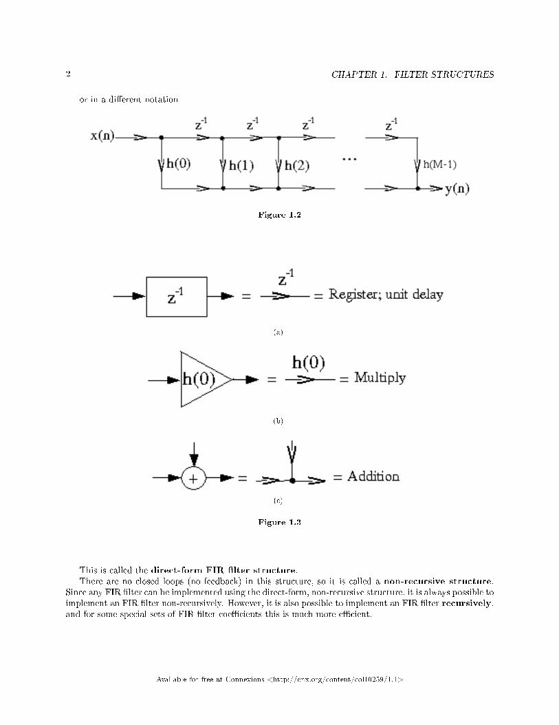
or in a di�erent notation

Figure 1.2

(a)

(b)

(c)

Figure 1.3

This is called the direct-form FIR �lter structure.There are no closed loops (no feedback) in this structure, so it is called a non-recursive structure.

Since any FIR �lter can be implemented using the direct-form, non-recursive structure, it is always possible toimplement an FIR �lter non-recursively. However, it is also possible to implement an FIR �lter recursively,and for some special sets of FIR �lter coe�cients this is much more e�cient.


3

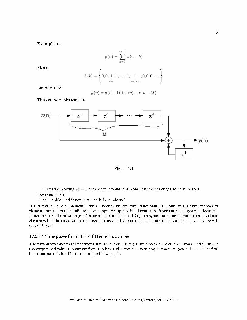
Example 1.1

y (n) =M−1∑k=0

x (n− k)

where

h (k) =

0, 0, 1ˆ

k=0

, 1, . . . , 1, 1ˆ

k=M−1

, 0, 0, 0, . . .

But note that

y (n) = y (n− 1) + x (n)− x (n−M)

This can be implemented as

Figure 1.4

Instead of costing M − 1 adds/output point, this comb �lter costs only two adds/output.

Exercise 1.2.1Is this stable, and if not, how can it be made so?

IIR �lters must be implemented with a recursive structure, since that's the only way a �nite number ofelements can generate an in�nite-length impulse response in a linear, time-invariant (LTI) system. Recursivestructures have the advantages of being able to implement IIR systems, and sometimes greater computationale�ciency, but the disadvantages of possible instability, limit cycles, and other deletorious e�ects that we willstudy shortly.

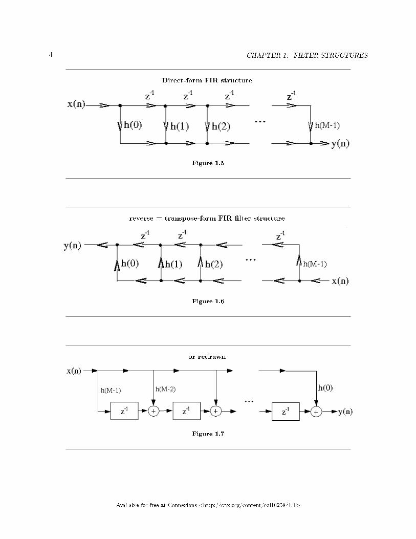
1.2.1 Transpose-form FIR �lter structures

The �ow-graph-reversal theorem says that if one changes the directions of all the arrows, and inputs atthe output and takes the output from the input of a reversed �ow-graph, the new system has an identicalinput-output relationship to the original �ow-graph.



Direct-form FIR structure

Figure 1.5

reverse = transpose-form FIR �lter structure

Figure 1.6

or redrawn

Figure 1.7


5

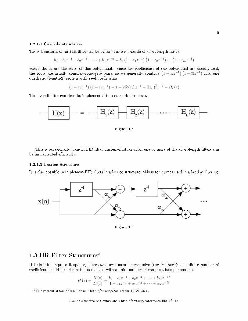
1.2.1.1 Cascade structures

The z-transform of an FIR �lter can be factored into a cascade of short-length �lters

b0 + b1z−1 + b2z

−3 + · · ·+ bmz−m = b0

(1− z1z

−1) (

1− z2z−1). . .(1− zmz−1

)where the zi are the zeros of this polynomial. Since the coe�cients of the polynomial are usually real,the roots are usually complex-conjugate pairs, so we generally combine

(1− ziz−1

) (1− ziz−1

)into one

quadratic (length-2) section with real coe�cients(1− ziz−1

) (1− ziz−1

)= 1− 2< (zi) z−1 + (|zi|)2

z−2 = Hi (z)

The overall �lter can then be implemented in a cascade structure.

Figure 1.8

This is occasionally done in FIR �lter implementation when one or more of the short-length �lters canbe implemented e�ciently.

1.2.1.2 Lattice Structure

It is also possible to implement FIR �lters in a lattice structure: this is sometimes used in adaptive �ltering

Figure 1.9

1.3 IIR Filter Structures3

IIR (In�nite Impulse Response) �lter structures must be recursive (use feedback); an in�nite number ofcoe�cients could not otherwise be realized with a �nite number of computations per sample.

H (z) =N (z)D (z)

=b0 + b1z

−1 + b2z−2 + · · ·+ bMz

−M

1 + a1z−1 + a2z−2 + · · ·+ aNz−N

3This content is available online at <http://cnx.org/content/m11919/1.2/>.



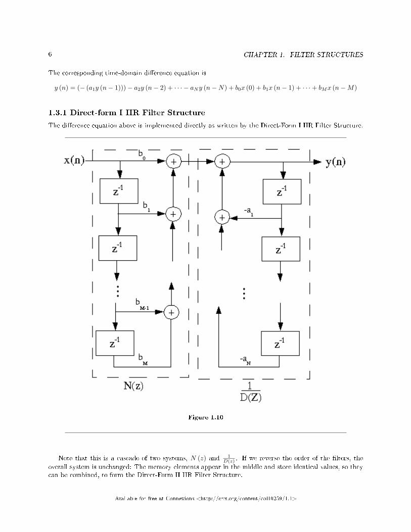
The corresponding time-domain di�erence equation is

y (n) = (− (a1y (n− 1)))− a2y (n− 2) + · · · − aNy (n−N) + b0x (0) + b1x (n− 1) + · · ·+ bMx (n−M)

1.3.1 Direct-form I IIR Filter Structure

The di�erence equation above is implemented directly as written by the Direct-Form I IIR Filter Structure.

Figure 1.10

Note that this is a cascade of two systems, N (z) and 1D(z) . If we reverse the order of the �lters, the

overall system is unchanged: The memory elements appear in the middle and store identical values, so theycan be combined, to form the Direct-Form II IIR Filter Structure.


7

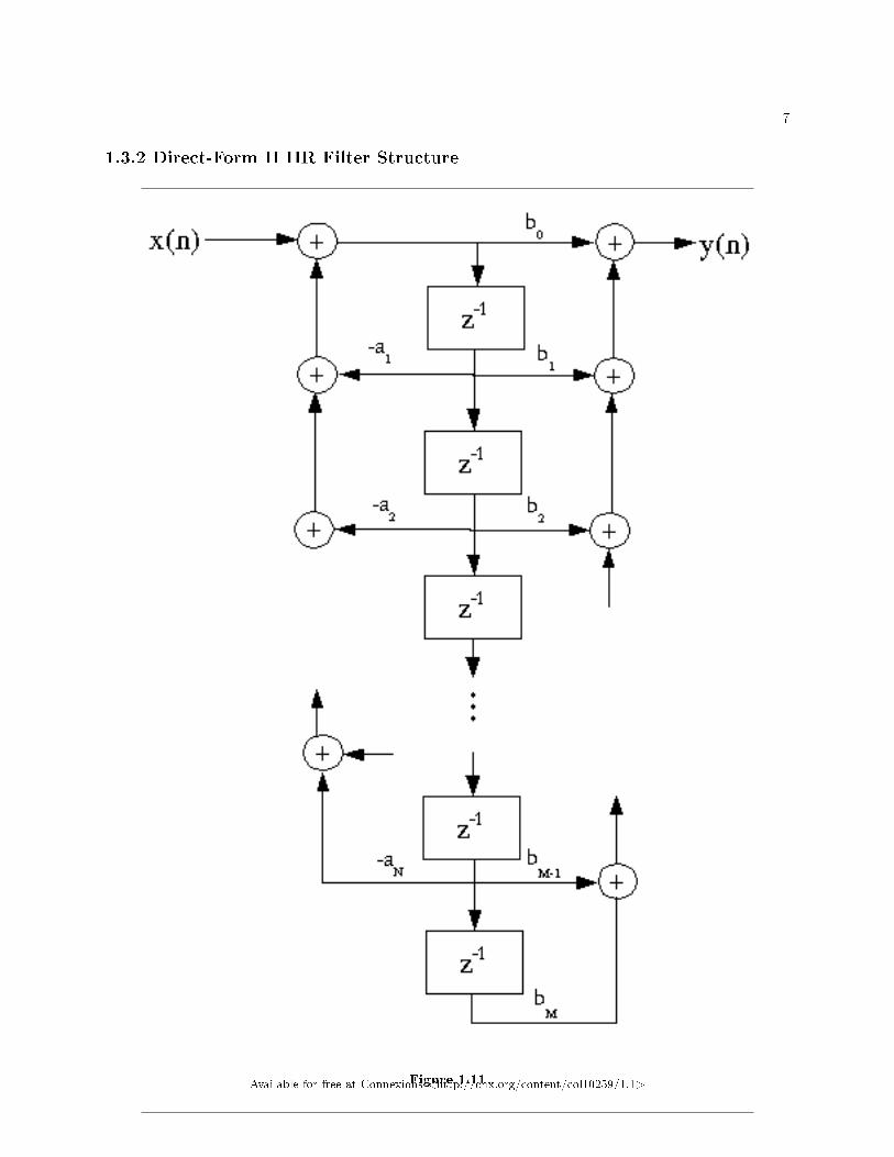
1.3.2 Direct-Form II IIR Filter Structure

Figure 1.11Available for free at Connexions <http://cnx.org/content/col10259/1.1>


This structure is canonic: (i.e., it requires the minimum number of memory elements).Flowgraph reversal gives the


9

1.3.3 Transpose-Form IIR Filter Structure

Figure 1.12



Usually we design IIR �lters with N = M , but not always.Obviously, since all these structures have identical frequency response, �lter structures are not unique.

We consider many di�erent structures because

1. Depending on the technology or application, one might be more convenient than another2. The response in a practical realization, in which the data and coe�cients must be quantized, may

di�er substantially, and some structures behave much better than others with quantization.

The Cascade-Form IIR �lter structure is one of the least sensitive to quantization, which is why it is themost commonly used IIR �lter structure.

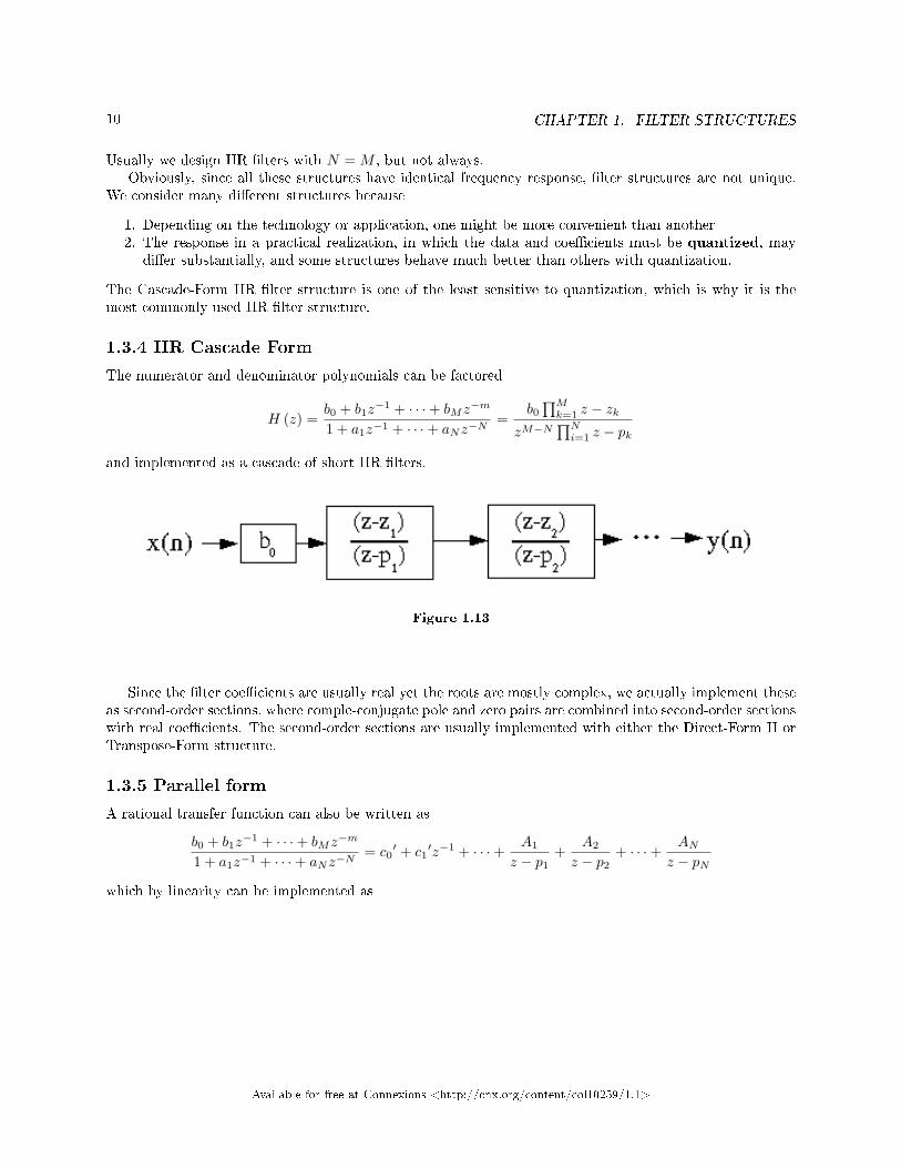
1.3.4 IIR Cascade Form

The numerator and denominator polynomials can be factored

H (z) =b0 + b1z

−1 + · · ·+ bMz−m

1 + a1z−1 + · · ·+ aNz−N=

b0∏Mk=1 z − zk

zM−N∏Ni=1 z − pk

and implemented as a cascade of short IIR �lters.

Figure 1.13

Since the �lter coe�cients are usually real yet the roots are mostly complex, we actually implement theseas second-order sections, where comple-conjugate pole and zero pairs are combined into second-order sectionswith real coe�cients. The second-order sections are usually implemented with either the Direct-Form II orTranspose-Form structure.

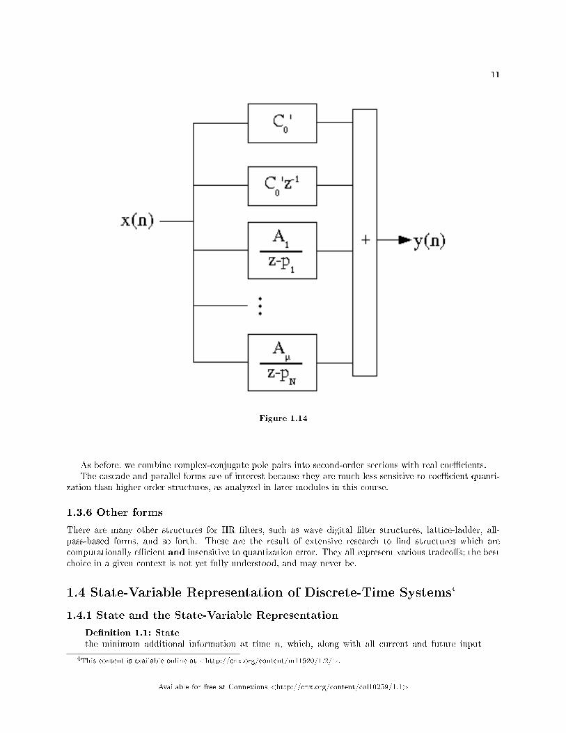
1.3.5 Parallel form

A rational transfer function can also be written as

b0 + b1z−1 + · · ·+ bMz

−m

1 + a1z−1 + · · ·+ aNz−N= c0

′ + c1′z−1 + · · ·+ A1

z − p1+

A2

z − p2+ · · ·+ AN

z − pN

which by linearity can be implemented as


11

Figure 1.14

As before, we combine complex-conjugate pole pairs into second-order sections with real coe�cients.The cascade and parallel forms are of interest because they are much less sensitive to coe�cient quanti-

zation than higher-order structures, as analyzed in later modules in this course.

1.3.6 Other forms

There are many other structures for IIR �lters, such as wave digital �lter structures, lattice-ladder, all-pass-based forms, and so forth. These are the result of extensive research to �nd structures which arecomputationally e�cient and insensitive to quantization error. They all represent various tradeo�s; the bestchoice in a given context is not yet fully understood, and may never be.

1.4 State-Variable Representation of Discrete-Time Systems4

1.4.1 State and the State-Variable Representation

De�nition 1.1: Statethe minimum additional information at time n, which, along with all current and future input




values, is necessary to compute all future outputs.

Essentially, the state of a system is the information held in the delay registers in a �lter structure orsignal �ow graph.

note: Any LTI (linear, time-invariant) system of �nite order M can be represented by a state-variable description

x (n+ 1) = Ax (n) +Bu (n)

y (n) = Cx (n) +Du (n)where x is an Mx1 "state vector," u (n) is the input at time n, y (n) is the output at time n; A isan MxM matrix, B is an Mx1 vector, C is a 1xM vector, and D is a 1x1 scalar.

One can always obtain a state-variable description of a signal �ow graph.

Example 1.2: 3rd-Order IIR

y (n) = (− (a1y (n− 1)))− a2y (n− 2)− a3y (n− 3) + b0x (n) + b1x (n− 1) + b2x (n− 2) + b3x (n− 3)

Figure 1.15


13

x1 (n+ 1)

x2 (n+ 1)

x3 (n+ 1)

=

0 1 0

0 0 1

−a3 −a2 −a1

x1 (n)

x2 (n)

x3 (n)

+

0

0

1

u (n)

y (n) =(− (a3b0) − (a2b0) − (a1b0)

)x1 (n)

x2 (n)

x3 (n)

+(b0

)u (n)

Exercise 1.4.1Is the state-variable description of a �lter H (z) unique?Exercise 1.4.2Does the state-variable description fully describe the signal �ow graph?

1.4.2 State-Variable Transformation

Suppose we wish to de�ne a new set of state variables, related to the old set by a linear transformation:q (n) = Tx (n), where T is a nonsingular MxM matrix, and q (n) is the new state vector. We wish theoverall system to remain the same. Note that x (n) = T−1q (n), and thus

x (n+ 1) = Ax (n) +Bu (n)⇒ T−1q (n) = AT−1q (n) +Bu (n)⇒ q (n) = TAT−1q (n) + TBu (n)

y (n) = Cx (n) +Du (n)⇒ y (n) = CT−1q (n) +Du (n)

This de�nes a new state system with an input-output behavior identical to the old system, but with di�erentinternal memory contents (states) and state matrices.

q (n) =^A q (n) +

^B u (n)

y (n) =^C q (n) +

^D u (n)

^A= TAT−1,

^B= TB,

^C= CT−1,

^D= D

These transformations can be used to generate a wide variety of alternative stuctures or implementationsof a �lter.

1.4.3 Transfer Function and the State-Variable Description

Taking the z transform of the state equations

Z [x (n+ 1)] = Z [Ax (n) +Bu (n)]

Z [y (n)] = Z [Cx (n) +Du (n)]

⇓

zX (z) = AX (z) +BU (z)



note: X (z) is a vector of scalar z-transforms X (z)T =(X1 (z) X2 (z) . . .

)Y (z) = CX (n) +DU (n)

(zI −A)X (z) = BU (z)⇒ X (z) = (zI −A)−1BU (z)

so

Y (z) = C(zI −A)−1BU (z) +DU (z)

=(C(− (zI))−1

B +D)U (z)

(1.1)

and thusH (z) = C(zI −A)−1

B +D

Note that since (zI −A)−1 =±(det(zI−A)red)T

det(z(I)−A) , this transfer function is an Mth-order rational fraction in z.

The denominator polynomial is D (z) = det (zI −A). A discrete-time state system is thus stable if the Mroots of det (zI −A) (i.e., the poles of the digital �lter) are all inside the unit circle.

Consider the transformed state system with^A= TAT−1,

^B= TB,

^C= CT−1,

^D= D:

H (z) =^C

(zI−

^A

)−1^B +

^D

= CT−1(zI − TAT−1

)−1TB +D

= CT−1(T (zI −A)T−1

)−1TB +D

= CT−1(T−1

)−1(zI −A)−1T−1TB +D

= C(zI −A)−1B +D

(1.2)

This proves that state-variable transformation doesn't change the transfer function of the underlying system.However, it can provide alternate forms that are less sensitive to coe�cient quantization or easier to analyze,understand, or implement.

State-variable descriptions of systems are useful because they provide a fairly general tool for analyzingall systems; they provide a more detailed description of a signal �ow graph than does the transfer function(although not a full description); and they suggest a large class of alternative implementations. They areeven more useful in control theory, which is largely based on state descriptions of systems.


Chapter 2

Fixed-Point Numbers

2.1 Fixed-Point Number Representation1

Fixed-point arithmetic is generally used when hardware cost, speed, or complexity is important. Finite-precision quantization issues usually arise in �xed-point systems, so we concentrate on �xed-point quanti-zation and error analysis in the remainder of this course. For basic signal processing computations such asdigital �lters and FFTs, the magnitude of the data, the internal states, and the output can usually be scaledto obtain good performance with a �xed-point implementation.

2.1.1 Two's-Complement Integer Representation

As far as the hardware is concerned, �xed-point number systems represent data as B-bit integers. Thetwo's-complement number system is usually used:

k =

binary integer representation if 0 ≤ k ≤ 2B−1 − 1

bit− by − bit inverse (−k) + 1 if − 2B−1 ≤ k ≤ 0

Figure 2.1

The most signi�cant bit is known at the sign bit; it is 0 when the number is non-negative; 1 when thenumber is negative.

2.1.2 Fractional Fixed-Point Number Representation

For the purposes of signal processing, we often regard the �xed-point numbers as binary fractions between[−1, 1), by implicitly placing a decimal point after the sign bit.



15

16 CHAPTER 2. FIXED-POINT NUMBERS

Figure 2.2

or

x = −b0 +B−1∑i=1

bi2−i

This interpretation makes it clearer how to implement digital �lters in �xed-point, at least when the coe�-cients have a magnitude less than 1.

2.1.3 Truncation Error

Consider the multiplication of two binary fractions

Figure 2.3

Note that full-precision multiplication almost doubles the number of bits; if we wish to return the productto a B-bit representation, we must truncate the B − 1 least signi�cant bits. However, this introducestruncation error (also known as quantization error, or roundo� error if the number is rounded to thenearest B-bit fractional value rather than truncated). Note that this occurs after multiplication.

2.1.4 Over�ow Error

Consider the addition of two binary fractions;

Figure 2.4

Note the occurence of wraparound over�ow; this only happens with addition. Obviously, it can be abad problem.

There are thus two types of �xed-point error: roundo� error, associated with data quantization andmultiplication, and over�ow error, associated with data quantization and additions. In �xed-point systems,one must strike a balance between these two error sources; by scaling down the data, the occurence ofover�ow errors is reduced, but the relative size of the roundo� error is increased.

note: Since multiplies require a number of additions, they are especially expensive in terms ofhardware (with a complexity proportional to BxBh, where Bx is the number of bits in the data,and Bh is the number of bits in the �lter coe�cients). Designers try to minimize both Bx and Bh,and often choose Bx 6= Bh!


17

2.2 Fixed-Point Quantization2

The fractional B-bit two's complement number representation evenly distributes 2B quantization levelsbetween −1 and 1− 2−(B−1). The spacing between quantization levels is then

22B

= 2−(B−1) .= ∆B

Any signal value falling between two levels is assigned to one of the two levels.XQ = Q [x] is our notation for quantization. e = Q [x]− x is then the quantization error.One method of quantization is rounding, which assigns the signal value to the nearest level. The

maximum error is thus ∆B

2 = 2−B .

(a) (b)

Figure 2.5

Another common scheme, which is often easier to implement in hardware, is truncation. Q [x] assignsx to the next lowest level.

(a) (b)

Figure 2.6



18 CHAPTER 2. FIXED-POINT NUMBERS

The worst-case error with truncation is ∆ = 2−(B−1), which is twice as large as with rounding. Also, theerror is always negative, so on average it may have a non-zero mean (i.e., a bias component).

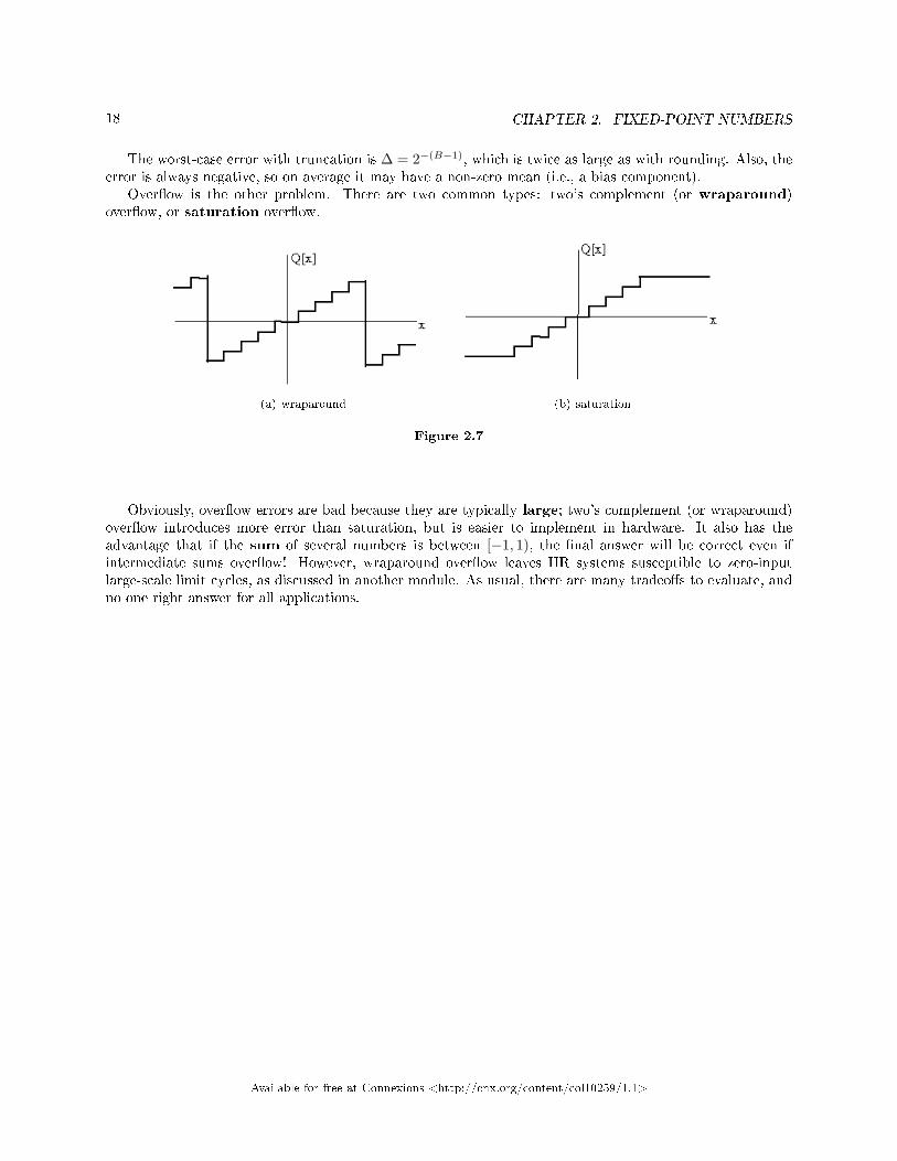
Over�ow is the other problem. There are two common types: two's complement (or wraparound)over�ow, or saturation over�ow.

(a) wraparound (b) saturation

Figure 2.7

Obviously, over�ow errors are bad because they are typically large; two's complement (or wraparound)over�ow introduces more error than saturation, but is easier to implement in hardware. It also has theadvantage that if the sum of several numbers is between [−1, 1), the �nal answer will be correct even ifintermediate sums over�ow! However, wraparound over�ow leaves IIR systems susceptible to zero-inputlarge-scale limit cycles, as discussed in another module. As usual, there are many tradeo�s to evaluate, andno one right answer for all applications.


Chapter 3

Quantization Error Analysis

3.1 Finite-Precision Error Analysis1

3.1.1 Fundamental Assumptions in �nite-precision error analysis

Quantization is a highly nonlinear process and is very di�cult to analyze precisely. Approximations andassumptions are made to make analysis tractable.

3.1.1.1 Assumption #1

The roundo� or truncation errors at any point in a system at each time are random, stationary, andstatistically independent (white and independent of all other quantizers in a system).

That is, the error autocorrelation function is re [k] = E [enen+k] = σq2δ [k]. Intuitively, and con�rmed

experimentally in some (but not all!) cases, one expects the quantization error to have a uniform distributionover the interval

[−∆

2 ,∆2

)for rounding, or (−∆, 0] for truncation.

In this case, rounding has zero mean and variance

E [Q [xn]− xn] = 0

σQ2 = E

[en

2]

=∆B

2

12and truncation has the statistics

E [Q [xn]− xn] = −∆2

σQ2 =

∆B2

12Please note that the independence assumption may be very bad (for example, when quantizing a sinusoid

with an integer period N). There is another quantizing scheme called dithering, in which the values arerandomly assigned to nearby quantization levels. This can be (and often is) implemented by adding a small(one- or two-bit) random input to the signal before a truncation or rounding quantizer.



19

20 CHAPTER 3. QUANTIZATION ERROR ANALYSIS

Figure 3.1

This is used extensively in practice. Altough the overall error is somewhat higher, it is spread evenly overall frequencies, rather than being concentrated in spectral lines. This is very important when quantizingsinusoidal or other periodic signals, for example.

3.1.1.2 Assumption #2

Pretend that the quantization error is really additive Gaussian noise with the same mean and variance asthe uniform quantizer. That is, model

(a)

(b) as

Figure 3.2

This model is a linear system, which our standard theory can handle easily. We model the noiseas Gaussian because it remains Gaussian after passing through �lters, so analysis in a system context istractable.


21

3.1.2 Summary of Useful Statistical Facts

• correlation function - rx [k] .= E [xnxn+k]• power spectral density - Sx (w) .= DTFT [rx [n]]• Note rx [0] = σx

2 = 12π

∫ π−π Sx (w) dw

• rxy [k] .= E [x∗ [n] y [n+ k]]• cross-spectral density - Sxy (w) = DTFT [rxy [n]]• For y = h ∗ x:

Syx (w) = H (w)Sx (w)

Syy (w) = (|H (w) |)2Sx (w)

• Note that the output noise level after �ltering a noise sequence is

σy2 = ryy [0] =

1π

∫ π

−π(|H (w) |)2

Sx (w) dw

so post�ltering quantization noise alters the noise power spectrum and may change its variance!• For x1, x2 statistically independent

rx1+x2 [k] = rx1 [k] + rx2 [k]

Sx1+x2 (w) = Sx1 (w) + Sx2 (w)

• For independent random variablesσx1+x2

2 = σx12 + σx2

2

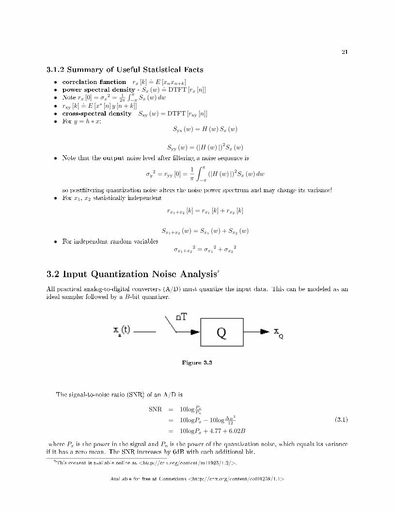
3.2 Input Quantization Noise Analysis2

All practical analog-to-digital converters (A/D) must quantize the input data. This can be modeled as anideal sampler followed by a B-bit quantizer.

Figure 3.3

The signal-to-noise ratio (SNR) of an A/D is

SNR = 10log Px

Pn

= 10logPx − 10log ∆B2

12

= 10logPx + 4.77 + 6.02B

(3.1)

where Px is the power in the signal and Pn is the power of the quantization noise, which equals its varianceif it has a zero mean. The SNR increases by 6dB with each additional bit.




3.3 Quantization Error in FIR Filters3

In digital �lters, both the data at various places in the �lter, which are continually varying, and the coef-�cients, which are �xed, must be quantized. The e�ects of quantization on data and coe�cients are quitedi�erent, so they are analyzed separately.

3.3.1 Data Quantization

Typically, the input and output in a digital �lter are quantized by the analog-to-digital and digital-to-analogconverters, respectively. Quantization also occurs at various points in a �lter structure, usually after amultiply, since multiplies increase the number of bits.

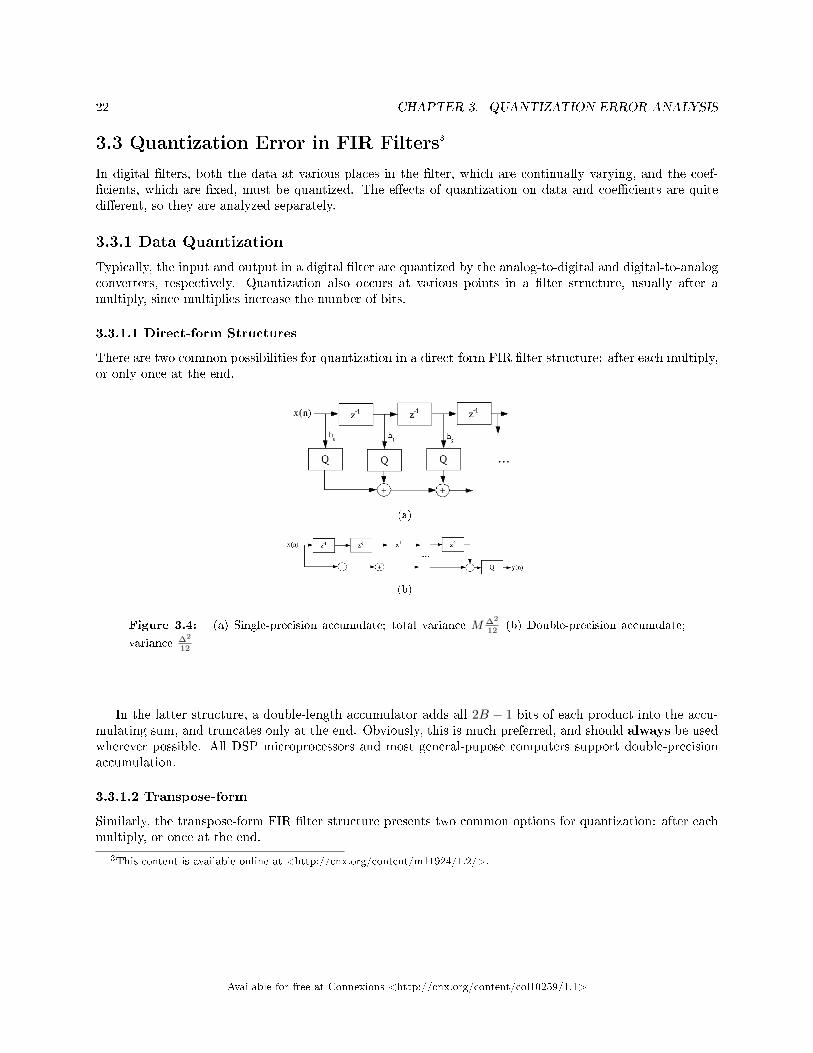
3.3.1.1 Direct-form Structures

There are two common possibilities for quantization in a direct-form FIR �lter structure: after each multiply,or only once at the end.

(a)

(b)

Figure 3.4: (a) Single-precision accumulate; total variance M ∆2

12(b) Double-precision accumulate;

variance ∆2

12

In the latter structure, a double-length accumulator adds all 2B − 1 bits of each product into the accu-mulating sum, and truncates only at the end. Obviously, this is much preferred, and should always be usedwherever possible. All DSP microprocessors and most general-pupose computers support double-precisionaccumulation.

3.3.1.2 Transpose-form

Similarly, the transpose-form FIR �lter structure presents two common options for quantization: after eachmultiply, or once at the end.



23

(a)

(b) or

Figure 3.5: (a) Quantize at each stage before storing intermediate sum. Output variance M ∆2

12(b)

Store double-precision partial sums. Costs more memory, but variance ∆2

12

The transpose form is not as convenient in terms of supporting double-precision accumulation, which isa signi�cant disadvantage of this structure.

3.3.2 Coe�cient Quantization

Since a quantized coe�cient is �xed for all time, we treat it di�erently than data quantization. The funda-mental question is: how much does the quantization a�ect the frequency response of the �lter?

The quantized �lter frequency response is

DTFT [hQ] = DTFT [hinf. prec. + e] = Hinf. prec. (w) +He (w)

Assuming the quantization model is correct, He (w) should be fairly random and white, with the error spreadfairly equally over all frequencies w ∈ [−π, π); however, the randomness of this error destroys any equirippleproperty or any in�nite-precision optimality of a �lter.

Exercise 3.3.1What quantization scheme minimizes the L2 quantization error in frequency (minimizes∫ π−π (|H (w)−HQ (w) |)2

dw)? On average, how big is this error?

Ideally, if one knows the coe�cients are to be quantized to B bits, one should incorporate this directlyinto the �lter design problem, and �nd the M B-bit binary fractional coe�cients minimizing the maximumdeviation (L∞ error). This can be done, but it is an integer program, which is known to be np-hard (i.e.,requires almost a brute-force search). This is so expensive computationally that it's rarely done. There aresome sub-optimal methods that are much more e�cient and usually produce pretty good results.

3.4 Data Quantization in IIR Filters4

Finite-precision e�ects are much more of a concern with IIR �lters than with FIR �lters, since the e�ectsare more di�cult to analyze and minimize, coe�cient quantization errors can cause the �lters to becomeunstable, and disastrous things like large-scale limit cycles can occur.




3.4.1 Roundo� noise analysis in IIR �lters

Suppose there are several quantization points in an IIR �lter structure. By our simplifying assumptionsabout quantization error and Parseval's theorem, the quantization noise variance σy,i

2 at the output of the�lter from the ith quantizer is

σy,i2 = 1

2π

∫ π−π (|Hi (w) |)2

SSni(w) dw

= σni2

2π

∫ π−π (|Hi (w) |)2

dw

= σni2∑∞n=−∞ hi

2 (n)

(3.2)

where σni2 is the variance of the quantization error at the ith quantizer, SSni

(w) is the power spectraldensity of that quantization error, and HHi (w) is the transfer function from the ith quantizer to the outputpoint. Thus for P independent quantizers in the structure, the total quantization noise variance is

σy2 =

12π

P∑i=1

σni

2

∫ π

−π(|Hi (w) |)2

dw

Note that in general, each Hi (w), and thus the variance at the output due to each quantizer, is di�erent;for example, the system as seen by a quantizer at the input to the �rst delay state in the Direct-Form II IIR�lter structure to the output, call it n4, is

Figure 3.6

with a transfer function

H4 (z) =z−2

1 + a1z−1 + a2z−2


25

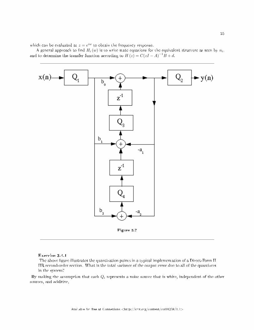
which can be evaluated at z = eiw to obtain the frequency response.A general approach to �nd Hi (w) is to write state equations for the equivalent structure as seen by ni,

and to determine the transfer function according to H (z) = C(zI −A)−1B + d.

Figure 3.7

Exercise 3.4.1The above �gure illustrates the quantization points in a typical implementation of a Direct-Form IIIIR second-order section. What is the total variance of the output error due to all of the quantizersin the system?

By making the assumption that each Qi represents a noise source that is white, independent of the othersources, and additive,



Figure 3.8

the variance at the output is the sum of the variances at the output due to each noise source:

σy2 =

4∑i=1

σy,i2

The variance due to each noise source at the output can be determined from 12π

∫ π−π (|Hi (w) |)2

Sni(w) dw;

note that Sni (w) = σni2 by our assumptions, and Hi (w) is the transfer function from the noise source

to the output.

3.5 IIR Coe�cient Quantization Analysis5

Coe�cient quantization is an important concern with IIR �lters, since straigthforward quantization oftenyields poor results, and because quantization can produce unstable �lters.

3.5.1 Sensitivity analysis

The performance and stability of an IIR �lter depends on the pole locations, so it is important to know howquantization of the �lter coe�cients ak a�ects the pole locations pj . The denominator polynomial is

D (z) = 1 +N∑k=1

akz−k =

N∏i=1

1− piz−1

We wish to know ∂pi

∂ak, which, for small deviations, will tell us that a δ change in ak yields an ε = δ ∂pi

∂ak

change in the pole location. ∂pi

∂akis the sensitivity of the pole location to quantization of ak. We can �nd

∂pi

∂akusing the chain rule.

∂A (z)∂ak

|z=pi=∂A (z)∂z

∂z

∂ak|z=pi

⇓

∂pi∂ak

=∂A(zi)∂ak

|z=pi

∂A(zi)∂z |z=pi



27

which is∂pi

∂ak= z−k

−(z−1QN

j=j 6=i,1 1−pjz−1) |z=pi

= −piN−kQN

j=j 6=i,1 pj−pi

(3.3)

Note that as the poles get closer together, the sensitivity increases greatly. So as the �lter order increases andmore poles get stu�ed closer together inside the unit circle, the error introduced by coe�cient quantizationin the pole locations grows rapidly.

How can we reduce this high sensitivity to IIR �lter coe�cient quantization?

3.5.1.1 Solution

Cascade (Section 1.3.4: IIR Cascade Form) or parallel form (Section 1.3.5: Parallel form) implementations!The numerator and denominator polynomials can be factored o�-line at very high precision and groupedinto second-order sections, which are then quantized section by section. The sensitivity of the quantizationis thus that of second-order, rather than N -th order, polynomials. This yields major improvements in thefrequency response of the overall �lter, and is almost always done in practice.

Note that the numerator polynomial faces the same sensitivity issues; the cascade form also improvesthe sensitivity of the zeros, because they are also factored into second-order terms. However, in the parallelform, the zeros are globally distributed across the sections, so they su�er from quantization of all the blocks.Thus the cascade form preserves zero locations much better than the parallel form, which typically meansthat the stopband behavior is better in the cascade form, so it is most often used in practice.

note: On the basis of the preceding analysis, it would seem important to use cascade structuresin FIR �lter implementations. However, most FIR �lters are linear-phase and thus symmetric oranti-symmetric. As long as the quantization is implemented such that the �lter coe�cients retainsymmetry, the �lter retains linear phase. Furthermore, since all zeros o� the unit circle mustappear in groups of four for symmetric linear-phase �lters, zero pairs can leave the unit circle onlyby joining with another pair. This requires relatively severe quantizations (enough to completelyremove or change the sign of a ripple in the amplitude response). This "reluctance" of pole pairsto leave the unit circle tends to keep quantization from damaging the frequency response as muchas might be expected, enough so that cascade structures are rarely used for FIR �lters.

Exercise 3.5.1 (Solution on p. 31.)

What is the worst-case pole pair in an IIR digital �lter?

3.5.2 Quantized Pole Locations

In a direct-form (Section 1.3.1: Direct-form I IIR Filter Structure) or transpose-form (Section 1.3.3:Transpose-Form IIR Filter Structure) implementation of a second-order section, the �lter coe�cients arequantized versions of the polynomial coe�cients.

D (z) = z2 + a1z + a2 = (z − p) (z − p)

p =−a1 ±

√a1

2 − 4a2

2

p = reiθ

D (z) = z2 − 2rcos (θ) + r2



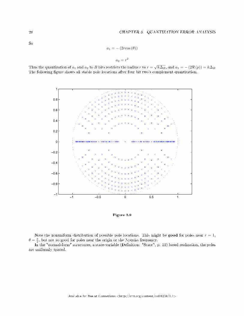
Soa1 = − (2rcos (θ))

a2 = r2

Thus the quantization of a1 and a2 to B bits restricts the radius r to r =√k∆B , and a1 = − (2< (p)) = k∆B

The following �gure shows all stable pole locations after four-bit two's-complement quantization.

Figure 3.9

Note the nonuniform distribution of possible pole locations. This might be good for poles near r = 1,θ = π

2 , but not so good for poles near the origin or the Nyquist frequency.In the "normal-form" structures, a state-variable (De�nition: "State", p. 11) based realization, the poles

are uniformly spaced.


29

Figure 3.10

This can only be accomplished if the coe�cients to be quantized equal the real and imaginary parts ofthe pole location; that is,

α1 = rcos (θ) = < (r)

α2 = rsin (θ) = = (p)

This is the case for a 2nd-order system with the state matrix (Section 1.4.1: State and the State-Variable

Representation) A =

α1 α2

−α1 α1

: The denominator polynomial is

det (zI −A) = (z − α1)2 + α22

= z2 − 2α1z + α12 + α2

2

= z2 − 2rcos (θ) z + r2(cos2 (θ) + sin2 (θ)

)= z2 − 2rcos (θ) z + r2

(3.4)

Given any second-order �lter coe�cient set, we can write it as a state-space system (Section 1.4.1: Stateand the State-Variable Representation), �nd a transformation matrix (Section 1.4.2: State-Variable Trans-



formation) T such that^A= T−1AT is in normal form, and then implement the second-order section using a

structure corresponding to the state equations.The normal form has a number of other advantages; both eigenvalues are equal, so it minimizes the norm

of Ax, which makes over�ow less likely, and it minimizes the output variance due to quantization of the statevalues. It is sometimes used when minimization of �nite-precision e�ects is critical.

Exercise 3.5.2 (Solution on p. 31.)

What is the disadvantage of the normal form?


31

Solutions to Exercises in Chapter 3

Solution to Exercise 3.5.1 (p. 27)The pole pair closest to the real axis in the z-plane, since the complex-conjugate poles will be closest togetherand thus have the highest sensitivity to quantization.Solution to Exercise 3.5.2 (p. 30)It requires more computation. The general state-variable equation (De�nition: "State", p. 11) requiresnine multiplies, rather than the �ve used by the Direct-Form II (Section 1.3.2: Direct-Form II IIR FilterStructure) or Transpose-Form (Section 1.3.3: Transpose-Form IIR Filter Structure) structures.


Chapter 4

Over�ow Problems and Solutions

4.1 Limit Cycles1

4.1.1 Large-scale limit cycles

When over�ow occurs, even otherwise stable �lters may get stuck in a large-scale limit cycle, which is ashort-period, almost full-scale persistent �lter output caused by over�ow.

Example 4.1Consider the second-order system

H (z) =1

1− z−1 + 12z−2

Figure 4.1



33

34 CHAPTER 4. OVERFLOW PROBLEMS AND SOLUTIONS

with zero input and initial state values z0 [0] = 0.8, z1 [0] = −0.8. Note y [n] = z0 [n+ 1].The �lter is obviously stable, since the magnitude of the poles is 1√

2= 0.707, which is well inside

the unit circle. However, with wraparound over�ow, note that y [0] = z0 [1] = 45−

12

(− 4

5

)= 6

5 = − 45 ,

and that z0 [2] = y [1] =(− 4

5

)− 1

245 = − 6

5 = 45 , so y [n] = − 4

5 ,45 ,−

45 ,

45 , . . . even with zero input.

Clearly, such behavior is intolerable and must be prevented. Saturation arithmetic has been proved toprevent zero-input limit cycles, which is one reason why all DSP microprocessors support this feature. Inmany applications, this is considered su�cient protection. Scaling to prevent over�ow is another solution, ifas well the inital state values are never initialized to limit-cycle-producing values. The normal-form structurealso reduces the chance of over�ow.

4.1.2 Small-scale limit cycles

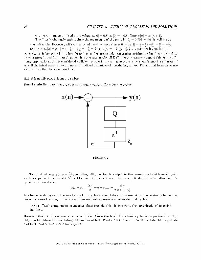
Small-scale limit cycles are caused by quantization. Consider the system

Figure 4.2

Note that when αz0 > z0− ∆B

2 , rounding will quantize the output to the current level (with zero input),so the output will remain at this level forever. Note that the maximum amplitude of this "small-scale limitcycle" is achieved when

αz0 = z0 −∆B

2=⇒= zmax =

∆B

2× (1− α)

In a higher-order system, the small-scale limit cycles are oscillatory in nature. Any quantization scheme thatnever increases the magnitude of any quantized value prevents small-scale limit cycles.

note: Two's-complement truncation does not do this; it increases the magnitude of negativenumbers.

However, this introduces greater error and bias. Since the level of the limit cycles is proportional to ∆B ,they can be reduced by increasing the number of bits. Poles close to the unit circle increase the magnitudeand likelihood of small-scale limit cycles.


35

4.2 Scaling2

Over�ow is clearly a serious problem, since the errors it introduces are very large. As we shall see, it is alsoresponsible for large-scale limit cycles, which cannot be tolerated. One way to prevent over�ow, or to renderit acceptably unlikely, is to scale the input to a �lter such that over�ow cannot (or is su�ciently unlikelyto) occur.

Figure 4.3

In a �xed-point system, the range of the input signal is limited by the fractional �xed-point numberrepresentation to |x [n] | ≤ 1. If we scale the input by multiplying it by a value β, 0 < β < 1, then|βx [n] | ≤ β.

Another option is to incorporate the scaling directly into the �lter coe�cients.

Figure 4.4

4.2.1 FIR Filter Scaling

What value of β is required so that the output of an FIR �lter cannot over�ow (∀n : (|y (n) | ≤ 1), ∀n :(|x (n) | ≤ 1))?

|y (n) | = |M−1∑k=0

h (k)βx (n− k) | ≤M−1∑k=0

|h (k) ||β||x (n− k) | ≤ βM−1∑k=0

|h (k) |1

⇓

β <

M−1∑k=0

|h (k) |



36 CHAPTER 4. OVERFLOW PROBLEMS AND SOLUTIONS

Alternatively, we can incorporate the scaling directly into the �lter, and require that

M−1∑k=0

|h (k) | < 1

to prevent over�ow.

4.2.2 IIR Filter Scaling

To prevent the output from over�owing in an IIR �lter, the condition above still holds: (M =∞)

|y (n) | <∞∑k=0

|h (k) |

so an initial scaling factor β < 1P∞k=0 |h(k)| can be used, or the �lter itself can be scaled.

However, it is also necessary to prevent the states from over�owing, and to prevent over�ow at any pointin the signal �ow graph where the arithmetic hardware would thereby produce errors. To prevent the statesfrom over�owing, we determine the transfer function from the input to all states i, and scale the �lter suchthat ∀i : (

∑∞k=0 |hi (k) | ≤ 1)

Although this method of scaling guarantees no over�ows, it is often too conservative. Note that a worst-case signal is x (n) = sign (h (−n)); this input may be extremely unlikely. In the relatively common situationin which the input is expected to be mainly a single-frequency sinusoid of unknown frequency and amplitudeless than 1, a scaling condition of

∀w : (|H (w) | ≤ 1)

is su�cient to guarantee no over�ow. This scaling condition is often used. If there are several potentialover�ow locations i in the digital �lter structure, the scaling conditions are

∀i, w : (|Hi (w) | ≤ 1)

where Hi (w) is the frequency response from the input to location i in the �lter.Even this condition may be excessively conservative, for example if the input is more-or-less random, or

if occasional over�ow can be tolerated. In practice, experimentation and simulation are often the best waysto optimize the scaling factors in a given application.

For �lters implemented in the cascade form, rather than scaling for the entire �lter at the beginning,(which introduces lots of quantization of the input) the �lter is usually scaled so that each stage is justprevented from over�owing. This is best in terms of reducing the quantization noise. The scaling factors areincorporated either into the previous or the next stage, whichever is most convenient.

Some heurisitc rules for grouping poles and zeros in a cascade implementation are:

1. Order the poles in terms of decreasing radius. Take the pole pair closest to the unit circle and groupit with the zero pair closest to that pole pair (to minimize the gain in that section). Keep doing thiswith all remaining poles and zeros.

2. Order the section with those with highest gain (argmax|Hi (w) |) in the middle, and those with lowergain on the ends.

Leland B. Jackson[1] has an excellent intuitive discussion of �nite-precision problems in digital �lters.The book by Roberts and Mullis[2] is one of the most thorough in terms of detail.


GLOSSARY 37

Glossary

S State

the minimum additional information at time n, which, along with all current and future inputvalues, is necessary to compute all future outputs.


38 BIBLIOGRAPHY


Bibliography

[1] Leland B. Jackson. Digital Filters and Signal Processing. Kluwer Academic Publishers, 2nd editionedition, 1989.

[2] Richard A. Roberts and Cli�ord T. Mullis. Digital Signal Processing. Prentice Hall, 1987.


39

40 INDEX

Index of Keywords and Terms

Keywords are listed by the section with that keyword (page numbers are in parentheses). Keywordsdo not necessarily appear in the text of the page. They are merely associated with that section. Ex.apples, � 1.1 (1) Terms are referenced by the page they appear on. Ex. apples, 1

C canonic, 8cascade, 5cascade form, � 1.3(5)cascade-form structure, � 3.5(26)coe�cient quantization, � 3.3(22), � 3.5(26)correlation function, � 3.1(19)

D data quantization, � 3.3(22)direct form, � 1.3(5), � 3.3(22)direct-form FIR �lter structure, 2direct-form structure, � 3.5(26)discrete-time systems, � 1.4(11)dithering, � 3.1(19), 19

F �lter structures, � 1.1(1)FIR, � 1.2(1)FIR �lters, � 3.3(22), � 4.2(35)�xed point, � 2.1(15)�ow-graph-reversal theorem, 3fractional number representation, � 2.1(15)

I IIR �lter quantization, � 3.5(26)IIR Filters, � 1.3(5), � 3.4(23), � 4.2(35)implementation, � 1.2(1)

L large-scale limit cycle, 33large-scale limit cycles, � 4.1(33)limit cycles, � 4.1(33)

N non-recursive structure, 2normal form, � 3.5(26)

O over�ow, � 2.1(15), 16, � 2.2(17), � 4.1(33),� 4.2(35)

P parallel form, � 1.3(5)power spectral density, � 3.1(19)

Q quantization, � 2.1(15), � 3.1(19), � 3.4(23)quantization error, 16, � 2.2(17), � 3.3(22)quantization noise, � 3.2(21)quantized, 10quantized pole locations, � 3.5(26)

R rounding, � 2.2(17), 17roundo� error, � 2.1(15), 16, � 2.2(17),� 3.1(19)roundo� noise analysis, � 3.4(23)

S saturation, � 2.2(17), 18scale, 35scaling, � 4.2(35)sensitivity, 26sensitivity analysis, � 3.5(26)sign bit, 15Signal-to-noise ratio, � 3.2(21)small-scale limit cycles, � 4.1(33), 34SNR, � 3.2(21)state, � 1.4(11), 11state space, � 1.4(11)state variable representation, � 1.4(11)state variable transformation, � 1.4(11)state variables, � 1.4(11)structures, � 1.2(1), � 1.3(5)

T transfer function, � 1.1(1)transpose form, � 1.3(5), � 3.3(22)transpose-form structure, � 3.5(26)truncation, � 2.1(15), � 2.2(17), 17truncation error, 16, � 2.2(17), � 3.1(19)two's complement, � 2.1(15)

W wraparound, 18wraparound error, � 2.2(17)

Z zero-input limit cycles, � 4.1(33), 34


ATTRIBUTIONS 41

Attributions

Collection: Digital Filter Structures and Quantization Error Analysis

Edited by: Douglas L. JonesURL: http://cnx.org/content/col10259/1.1/License: http://creativecommons.org/licenses/by/1.0

Module: "Filter Structures"By: Douglas L. JonesURL: http://cnx.org/content/m11917/1.3/Page: 1Copyright: Douglas L. JonesLicense: http://creativecommons.org/licenses/by/1.0

Module: "FIR Filter Structures"By: Douglas L. JonesURL: http://cnx.org/content/m11918/1.2/Pages: 1-5Copyright: Douglas L. JonesLicense: http://creativecommons.org/licenses/by/1.0

Module: "IIR Filter Structures"By: Douglas L. JonesURL: http://cnx.org/content/m11919/1.2/Pages: 5-11Copyright: Douglas L. JonesLicense: http://creativecommons.org/licenses/by/1.0

Module: "State-Variable Representation of Discrete-Time Systems"By: Douglas L. JonesURL: http://cnx.org/content/m11920/1.2/Pages: 11-14Copyright: Douglas L. JonesLicense: http://creativecommons.org/licenses/by/1.0

Module: "Fixed-Point Number Representation"By: Douglas L. JonesURL: http://cnx.org/content/m11930/1.2/Pages: 15-16Copyright: Douglas L. JonesLicense: http://creativecommons.org/licenses/by/1.0

Module: "Fixed-Point Quantization"By: Douglas L. JonesURL: http://cnx.org/content/m11921/1.2/Pages: 17-18Copyright: Douglas L. JonesLicense: http://creativecommons.org/licenses/by/1.0


42 ATTRIBUTIONS

Module: "Finite-Precision Error Analysis"By: Douglas L. JonesURL: http://cnx.org/content/m11922/1.2/Pages: 19-21Copyright: Douglas L. JonesLicense: http://creativecommons.org/licenses/by/1.0

Module: "Input Quantization Noise Analysis"By: Douglas L. JonesURL: http://cnx.org/content/m11923/1.2/Page: 21Copyright: Douglas L. JonesLicense: http://creativecommons.org/licenses/by/1.0

Module: "Quantization Error in FIR Filters"By: Douglas L. JonesURL: http://cnx.org/content/m11924/1.2/Pages: 22-23Copyright: Douglas L. JonesLicense: http://creativecommons.org/licenses/by/1.0

Module: "Data Quantization in IIR Filters"By: Douglas L. JonesURL: http://cnx.org/content/m11925/1.2/Pages: 23-26Copyright: Douglas L. JonesLicense: http://creativecommons.org/licenses/by/1.0

Module: "IIR Coe�cient Quantization Analysis"By: Douglas L. JonesURL: http://cnx.org/content/m11926/1.2/Pages: 26-30Copyright: Douglas L. JonesLicense: http://creativecommons.org/licenses/by/1.0

Module: "Limit Cycles"By: Douglas L. JonesURL: http://cnx.org/content/m11928/1.2/Pages: 33-34Copyright: Douglas L. JonesLicense: http://creativecommons.org/licenses/by/1.0

Module: "Scaling"By: Douglas L. JonesURL: http://cnx.org/content/m11927/1.2/Pages: 35-36Copyright: Douglas L. JonesLicense: http://creativecommons.org/licenses/by/1.0


Digital Filter Structures and Quantization Error AnalysisPractical implementations of digital �lters introduce errors due to �nite-precision data and arithmetic. Manydi�erent structures, both for FIR and IIR �lters, o�er di�erent trade-o�s between computational complexity,memory use, precision, and error. Approximating the errors as additive noise provides fairly accurateestimates of the resulting quantization noise levels, which can be used both to predict the performanceof a chosen implementation and to determine the precision needed to meet design requirements.

About ConnexionsSince 1999, Connexions has been pioneering a global system where anyone can create course materials andmake them fully accessible and easily reusable free of charge. We are a Web-based authoring, teaching andlearning environment open to anyone interested in education, including students, teachers, professors andlifelong learners. We connect ideas and facilitate educational communities.

Connexions's modular, interactive courses are in use worldwide by universities, community colleges, K-12schools, distance learners, and lifelong learners. Connexions materials are in many languages, includingEnglish, Spanish, Chinese, Japanese, Italian, Vietnamese, French, Portuguese, and Thai. Connexions is partof an exciting new information distribution system that allows for Print on Demand Books. Connexionshas partnered with innovative on-demand publisher QOOP to accelerate the delivery of printed coursematerials and textbooks into classrooms worldwide at lower prices than traditional academic publishers.

digital filter structures and quantization error analysis1.1... · digital filter structures and...

Documents