differential evolution

IntroductionOptimization is viewed as a decision

problem that involves finding the best values of the decision variables over all possibilities.

The best values would give the smallest objective function value for a minimization problem or the largest objective function value for a maximization problem.

In terms of real world applications, the objective function is often a representation of some physically significant measure such as profit, loss, utility, risk or error.

Evolution in Biology

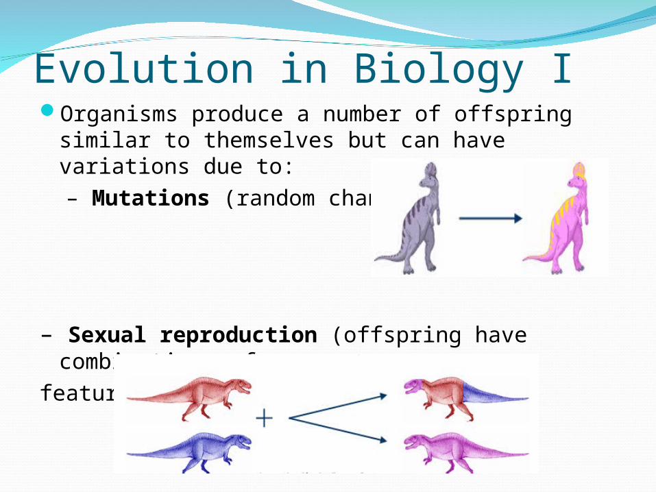
Evolution in Biology IOrganisms produce a number of offspring similar

to themselves but can have variations due to: – Mutations (random changes)

– Sexual reproduction (offspring have combinations of

features inherited from each parent)

Evolution in Biology IISome offspring survive, and produce next generations,

and some don’t:– The organisms adapted to the environment better have higher chance to survive– Over time, the generations become more and more adapted because the fittest organisms survive

Differential EvolutionPopulation-based optimisation algorithmIntroduced by Storn and Price in 1996But many practical problems have objective

functions that are non-differentiable, hence gradient based methods cannot be employed

Developed to optimise mixed integer-discrete-continuous non-linear programming as against the continuous non-linear programming which is done by most of the algorithms.

Why use Differential Evolution?All evolutionary algorithms use predefined

probability density functions(PDFs) for parameter perturbation. These PDFs have to be adapted throughout the optimization by a process that imposes additional complexity to the optimization procedures.

DE is a self-adjusting as it deduces the perturbation information from the distances between the vectors that comprise the population.

Problem

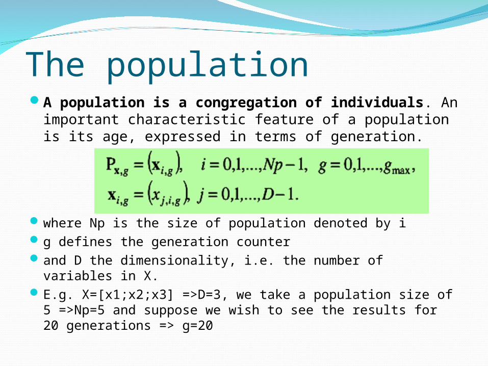
The populationA population is a congregation of individuals. An

important characteristic feature of a population is its age, expressed in terms of generation.

where Np is the size of population denoted by i g defines the generation counter and D the dimensionality, i.e. the number of variables in X.E.g. X=[x1;x2;x3] =>D=3, we take a population size of 5

=>Np=5 and suppose we wish to see the results for 20 generations => g=20

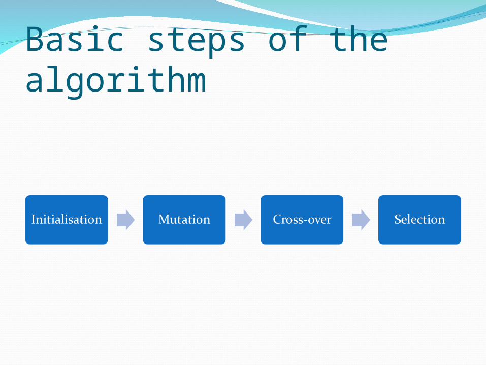
Basic steps of the algorithm

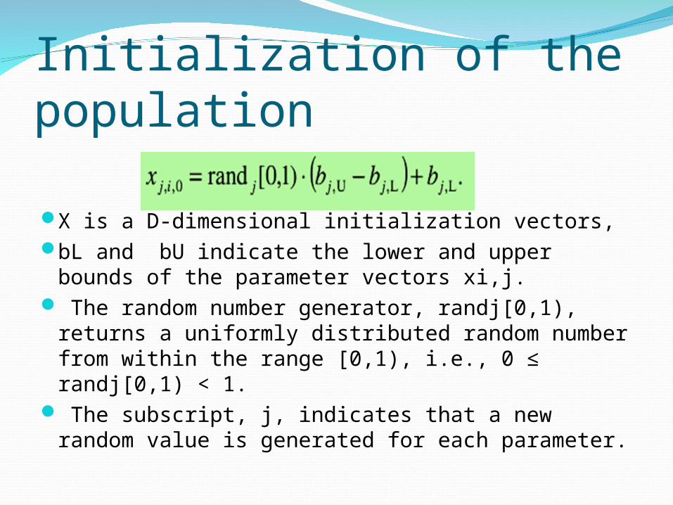
Initialization of the population

X is a D-dimensional initialization vectors, bL and bU indicate the lower and upper bounds

of the parameter vectors xi,j. The random number generator, randj[0,1),

returns a uniformly distributed random number from within the range [0,1), i.e., 0 ≤ randj[0,1) < 1.

The subscript, j, indicates that a new random value is generated for each parameter.

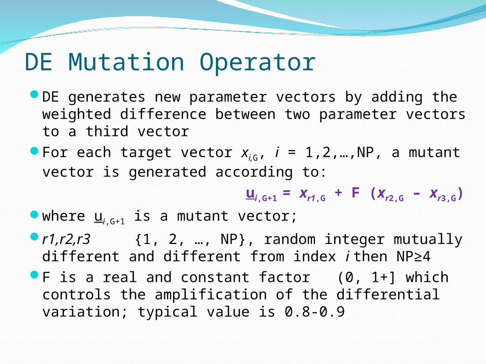
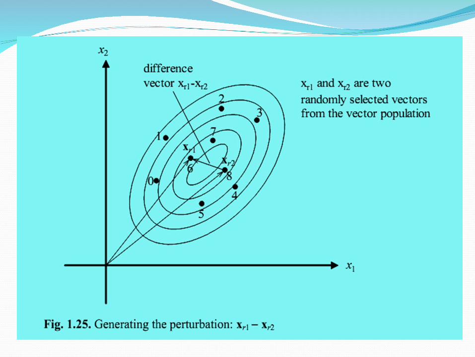
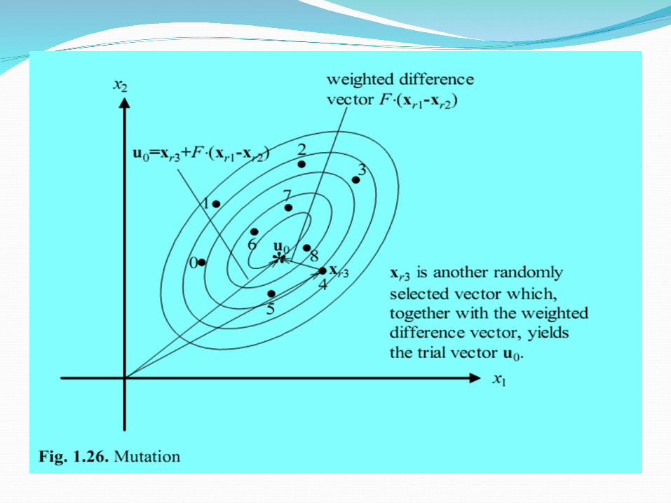
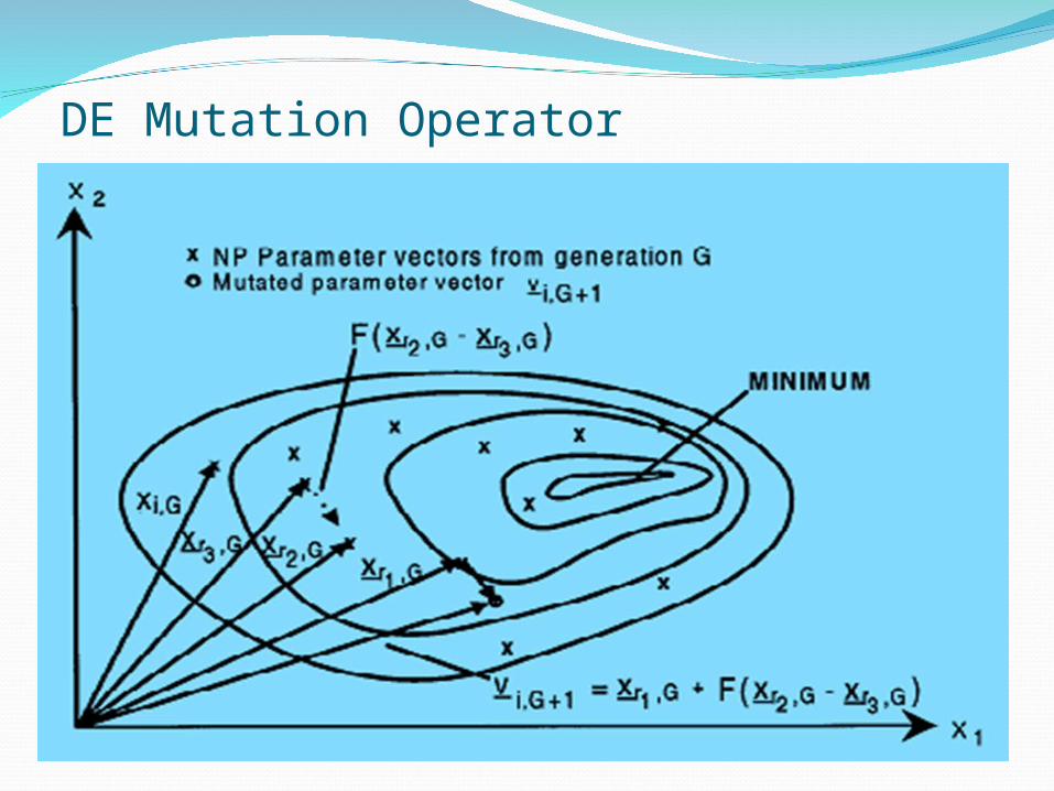
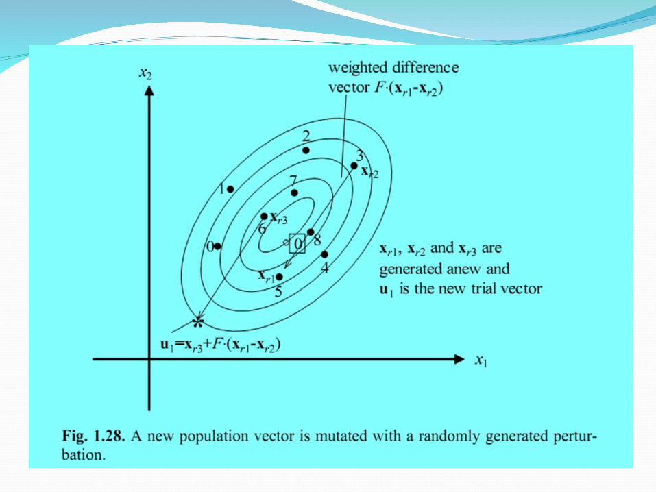
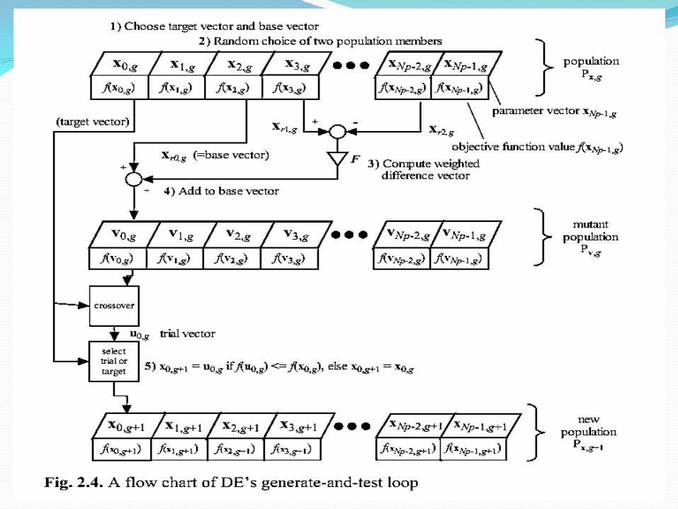
DE Mutation OperatorDE generates new parameter vectors by adding the

weighted difference between two parameter vectors to a third vector

For each target vector xi,G, i = 1,2,…,NP, a mutant vector is generated according to:

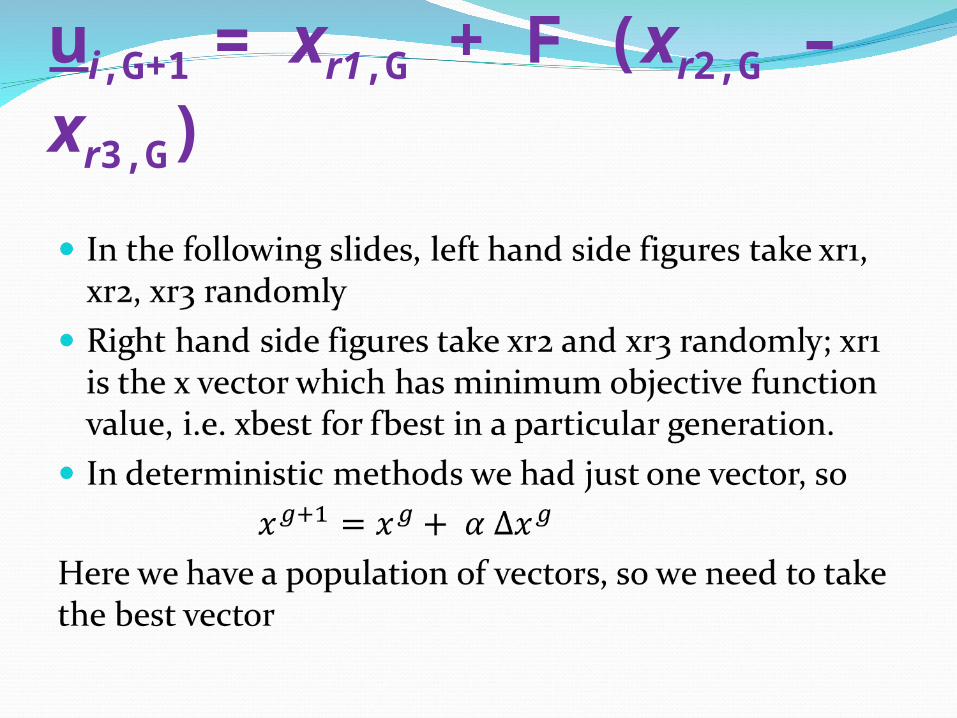
ui,G+1 = xr1,G + F (xr2,G – xr3,G)

where ui,G+1 is a mutant vector; r1,r2,r3 {1, 2, …, NP}, random integer mutually

different and different from index i then NP≥4F is a real and constant factor (0, 1+] which controls

the amplification of the differential variation; typical value is 0.8-0.9

DE Mutation Operator

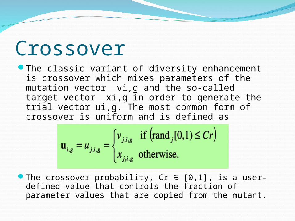
CrossoverThe classic variant of diversity enhancement is

crossover which mixes parameters of the mutation vector vi,g and the so-called target vector xi,g in order to generate the trial vector ui,g. The most common form of crossover is uniform and is defined as

The crossover probability, Cr ∈ [0,1], is a user-defined value that controls the fraction of parameter values that are copied from the mutant.

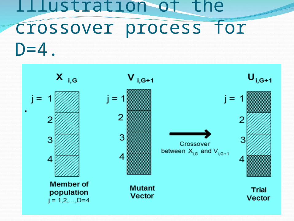
Illustration of the crossover process for D=4.

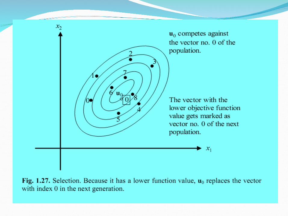
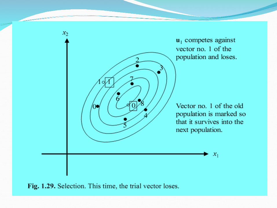
SelectionDE uses simple one-to-one survivor selection

where the trial vector ui,g competes against the target vector xi,g. The vector with the lowest objective function value survives into the next generation g+1

Termination criteriaa preset number of maximum generations,the difference between the best and worst

function values in the population is verysmall,the best function value has not improved

beyond some tolerance value for a predefined number of generations,

the distance between solution vectors in the population is small.

Intrinsic Control Parameters of Differential Evolution1. population size Np;2. mutation intensities Fy3. crossover probability pc

1. First Choice2. The originators recommend Np/N=10,

F=0.8, and pc =0.9. However, F=0.5 and pc=0.1 are also claimed to be a good first choice.

Adjusting Intrinsic Control ParametersDifferent problems usually require different

intrinsic control parameters.Increasing the population size is suggested

if differential evolution does not converge. However, this only helps to a certain extent.

Mutation intensity has to be adjusted a little lower or higher than 0.8 if population size is increased. It is claimed that convergence is more likely to occur but generally takes longer with larger population and weaker mutation (smaller F).

DE dynamicsThere are two opposing mechanisms that

influence DE’s population.1) Population tendency to expand and

explore the terrain on which it is working. It also prevents DE’s population from converging prematurely.

2)By selection, expansion is counteracted by removing vectors which are located in unproductive regions.

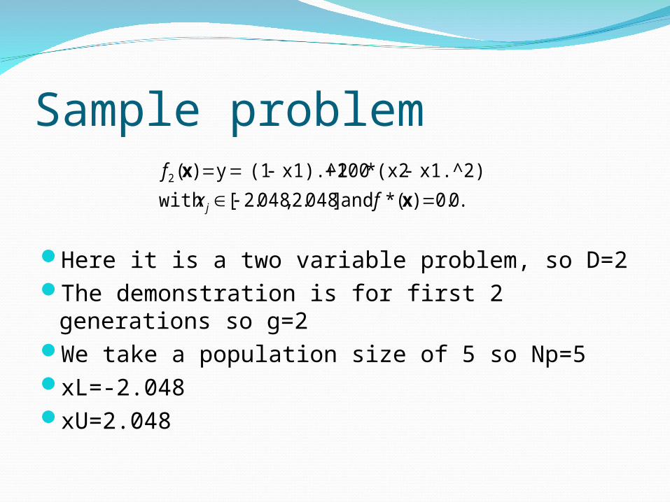
Sample problem

Here it is a two variable problem, so D=2The demonstration is for first 2 generations

so g=2We take a population size of 5 so Np=5xL=-2.048xU=2.048

.0.0)(* and ]048.2 ,048.2[with

x1.^2).^2- (x2*100 x1).^2- (1 y )(2

x

x

fx

f

j

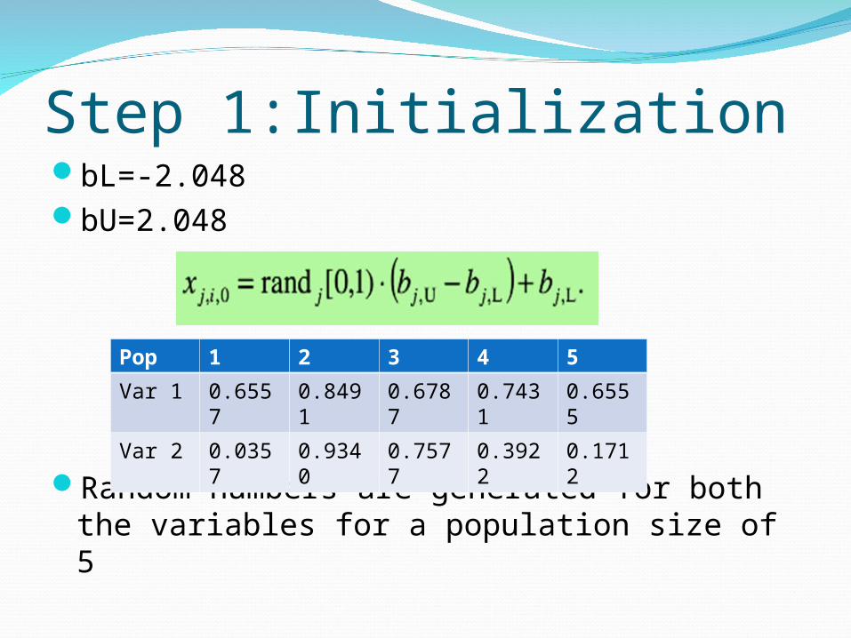
Step 1:InitializationbL=-2.048bU=2.048

Random numbers are generated for both the variables for a population size of 5

Pop 1 2 3 4 5

Var 1 0.6557

0.8491

0.6787

0.7431

0.6555

Var 2 0.0357

0.9340

0.7577

0.3922

0.1712

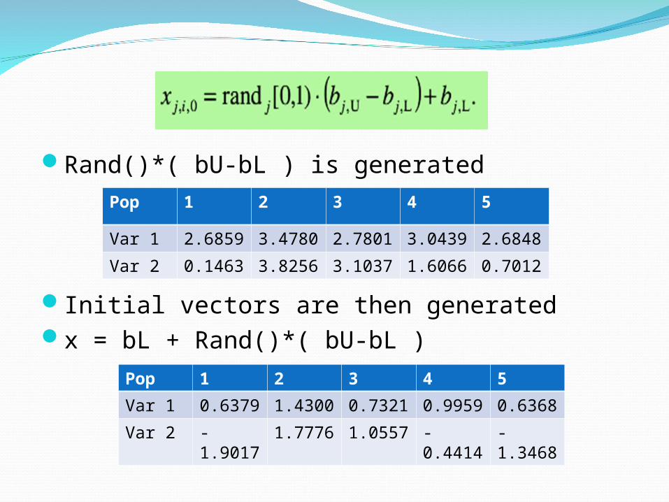
Rand()*( bU-bL ) is generated

Initial vectors are then generatedx = bL + Rand()*( bU-bL )

Pop 1 2 3 4 5

Var 1 2.6859 3.4780 2.7801 3.0439 2.6848

Var 2 0.1463 3.8256 3.1037 1.6066 0.7012

Pop 1 2 3 4 5

Var 1 0.6379 1.4300 0.7321 0.9959 0.6368

Var 2 -1.9017

1.7776 1.0557 -0.4414

-1.3468

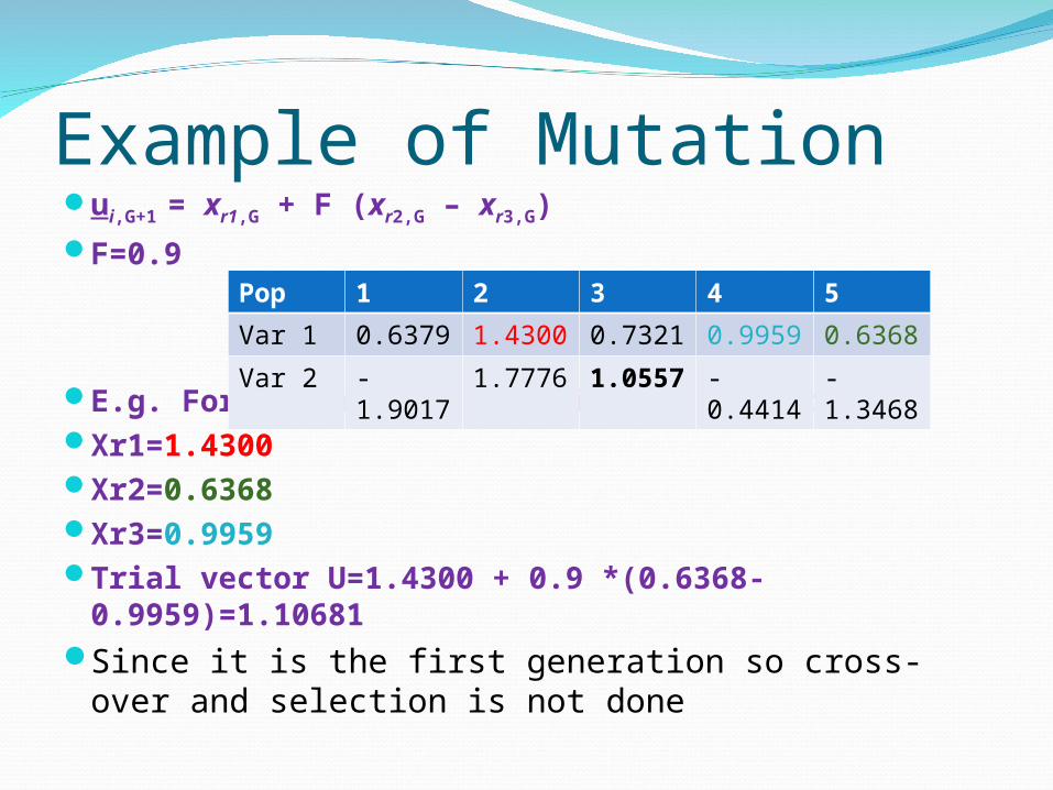
Example of Mutationui,G+1 = xr1,G + F (xr2,G – xr3,G)F=0.9

E.g. For 1st variable and first generationXr1=1.4300Xr2=0.6368Xr3=0.9959Trial vector U=1.4300 + 0.9 *(0.6368-

0.9959)=1.10681Since it is the first generation so cross-over and

selection is not done

Pop 1 2 3 4 5

Var 1 0.6379 1.4300 0.7321 0.9959 0.6368

Var 2 -1.9017

1.7776 1.0557

-0.4414

-1.3468

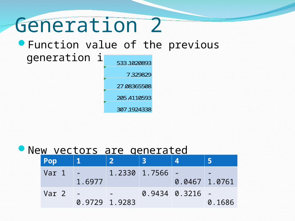
Generation 2Function value of the previous generation is

New vectors are generated

533.1020893

7.329829

27.08365508

205.4110593

307.1924338

Pop 1 2 3 4 5

Var 1 -1.6977

1.2330 1.7566 -0.0467

-1.0761

Var 2 -0.9729

-1.9283

0.9434 0.3216 -0.1686

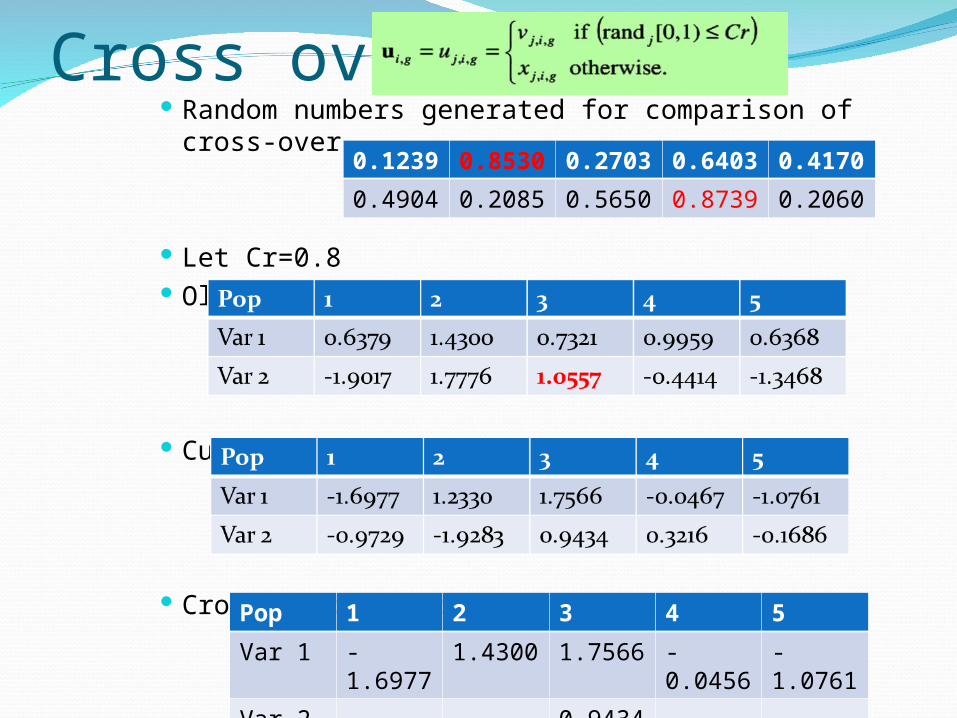
Cross over Random numbers generated for comparison of

cross-over

Let Cr=0.8 Old population

Current population x(i,2)

Crossed population u(i,2)

0.1239

0.8530

0.2703

0.6403

0.4170

0.4904 0.2085 0.5650 0.8739 0.2060

Pop 1 2 3 4 5

Var 1 -1.6977

1.4300 1.7566 -0.0456

-1.0761

Var 2 -0.9729

-1.9283

0.9434 -0.4414

-0.1686

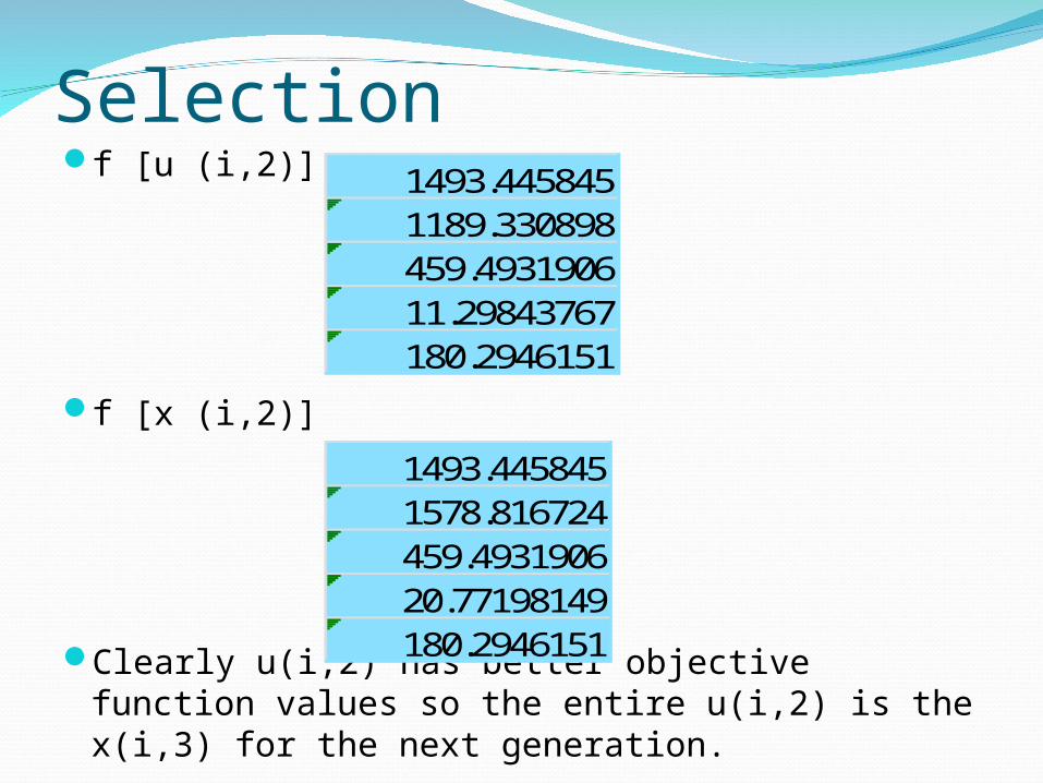
Selectionf [u (i,2)]

f [x (i,2)]

Clearly u(i,2) has better objective function values so the entire u(i,2) is the x(i,3) for the next generation.

1493.4458451189.330898459.493190611.29843767180.2946151

1493.4458451578.816724459.493190620.77198149180.2946151

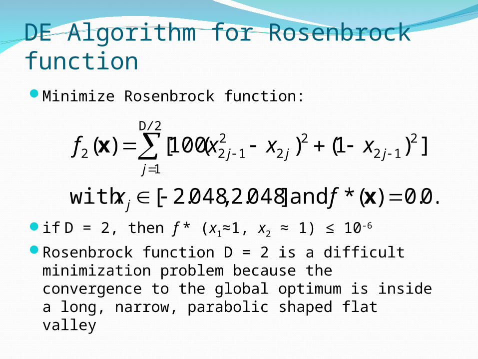
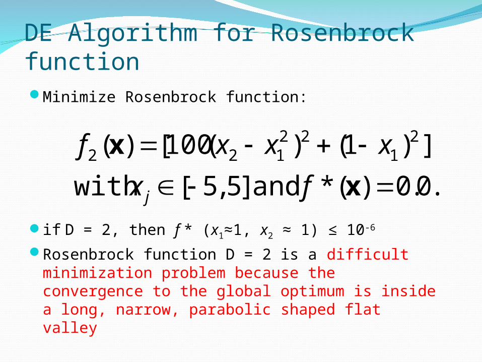
DE Algorithm for Rosenbrock functionMinimize Rosenbrock function:

if D = 2, then f * (x1≈1, x2 ≈ 1) ≤ 10-6

Rosenbrock function D = 2 is a difficult minimization problem because the convergence to the global optimum is inside a long, narrow, parabolic shaped flat valley

.0.0)(* and ]048.2 ,048.2[with

])1()(100[)( 212

22

212

2D

12

x

x

fx

xxxf

j

jjj

/

j

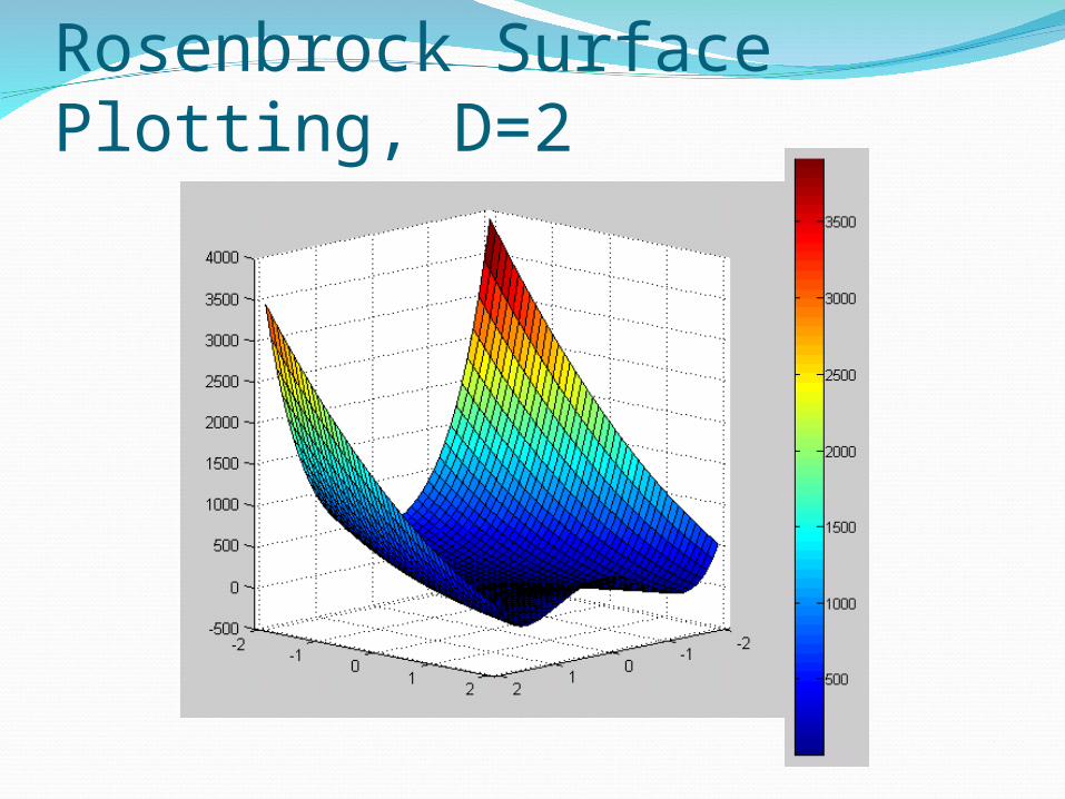
Rosenbrock Surface Plotting, D=2

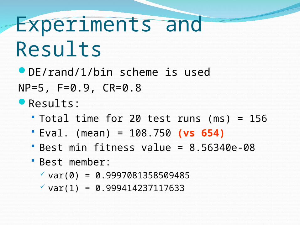
Experiments and ResultsDE/rand/1/bin scheme is usedNP=5, F=0.9, CR=0.8Results:

Total time for 20 test runs (ms) = 156 Eval. (mean) = 108.750 (vs 654) Best min fitness value = 8.56340e-08 Best member:

var(0) = 0.9997081358509485 var(1) = 0.999414237117633

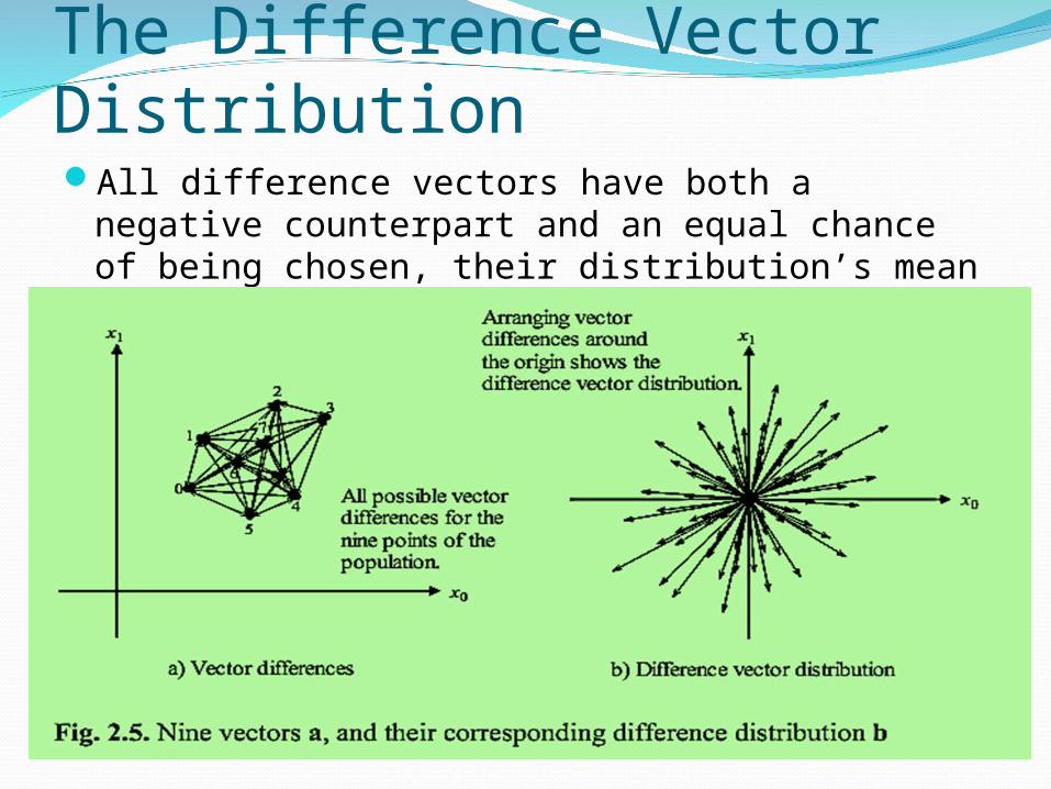
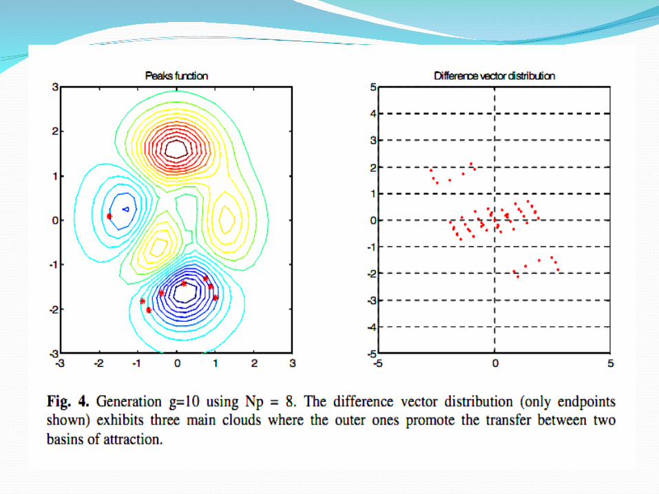
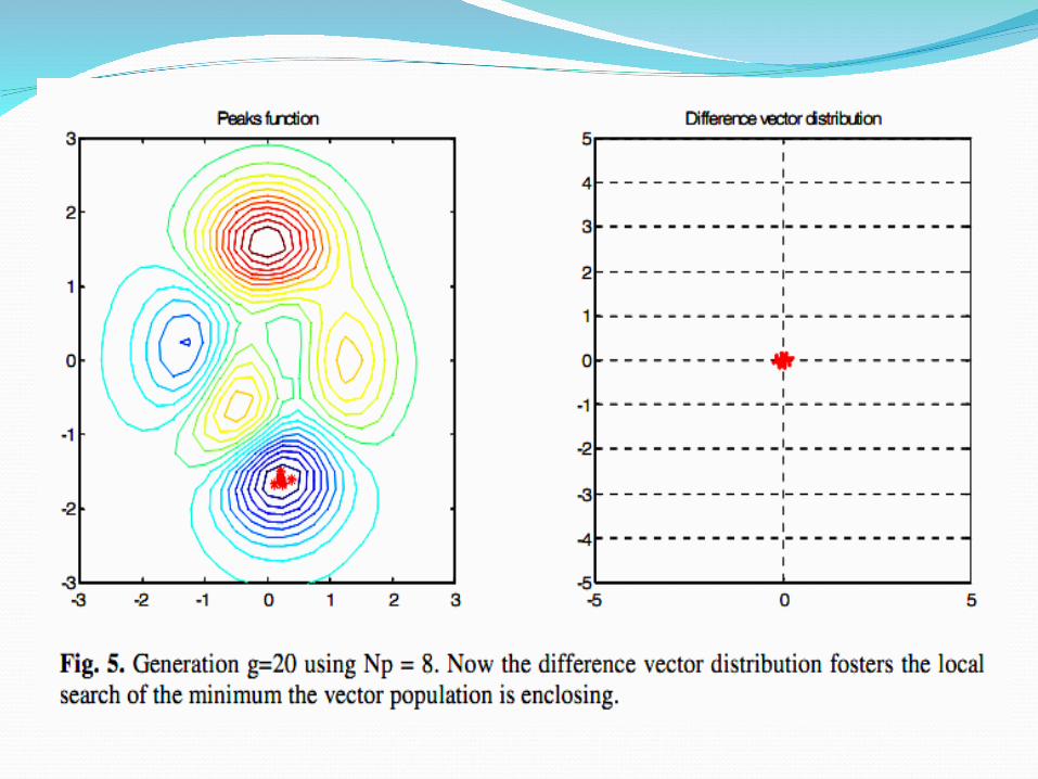
The Difference Vector Distribution All difference vectors have both a negative

counterpart and an equal chance of being chosen, their distribution’s mean is zero.

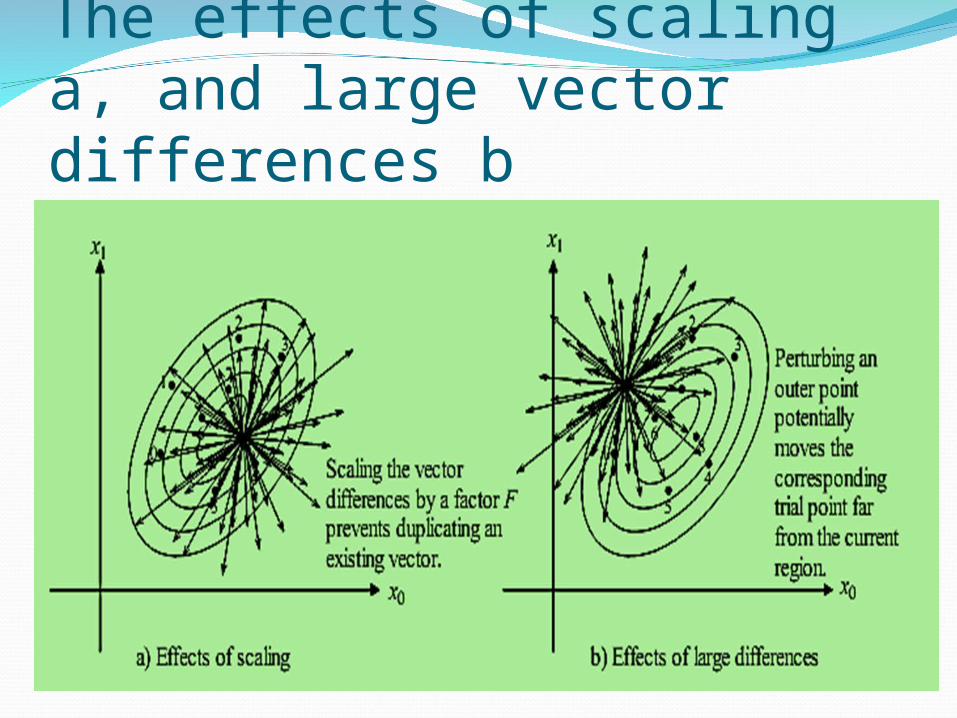
The effects of scaling a, and large vector differences b

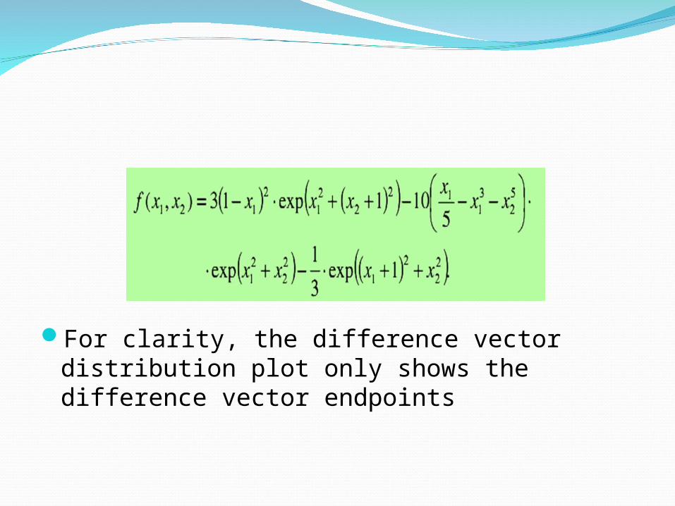
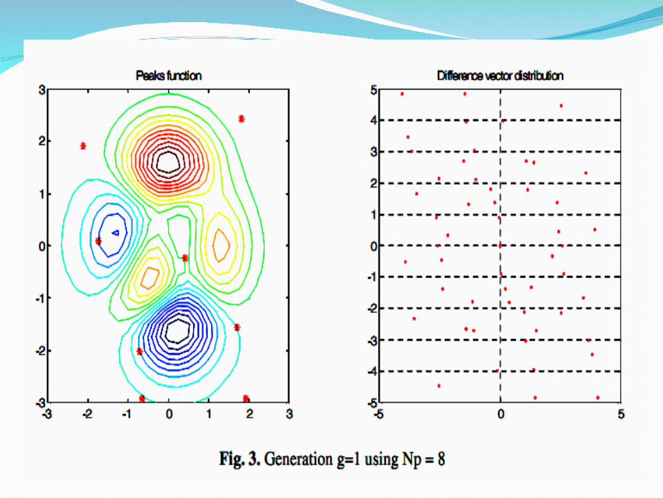
For clarity, the difference vector distribution plot only shows the difference vector endpoints

DE Algorithm for Rosenbrock functionMinimize Rosenbrock function:

if D = 2, then f * (x1≈1, x2 ≈ 1) ≤ 10-6

Rosenbrock function D = 2 is a difficult minimization problem because the convergence to the global optimum is inside a long, narrow, parabolic shaped flat valley

.0.0)(* and ]5 ,5[with

])1()(100[)( 21

22122

x

x

fx

xxxf

j

Rosenbrock Surface Plotting, D=2

ui,G+1 = xr1,G + F (xr2,G – xr3,G)

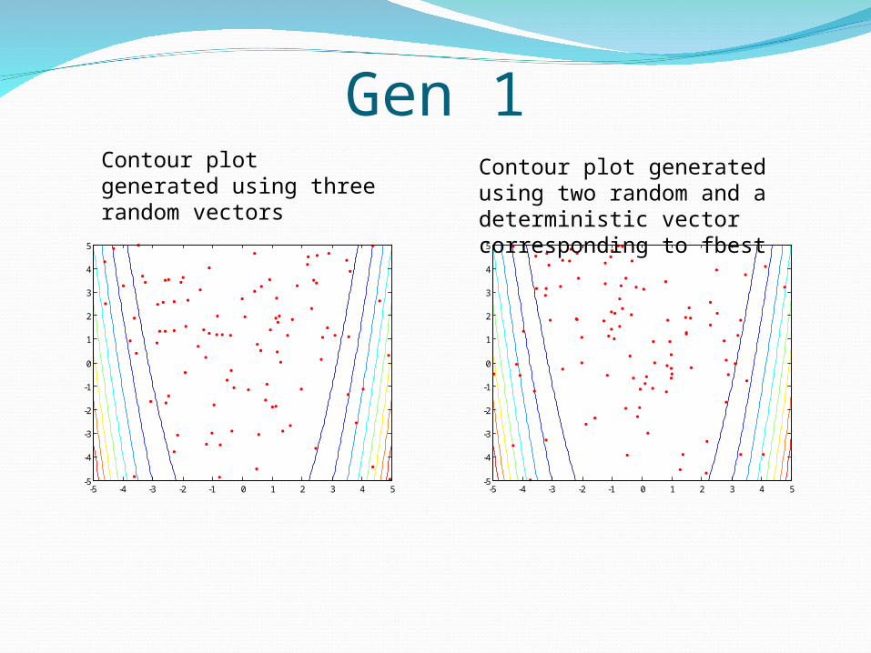
Gen 1

-5 -4 -3 -2 -1 0 1 2 3 4 5-5

-4

-3

-2

-1

0

1

2

3

4

5

-5 -4 -3 -2 -1 0 1 2 3 4 5-5

-4

-3

-2

-1

0

1

2

3

4

5

Contour plot generated using three random vectors

Contour plot generated using two random and a deterministic vector corresponding to fbest

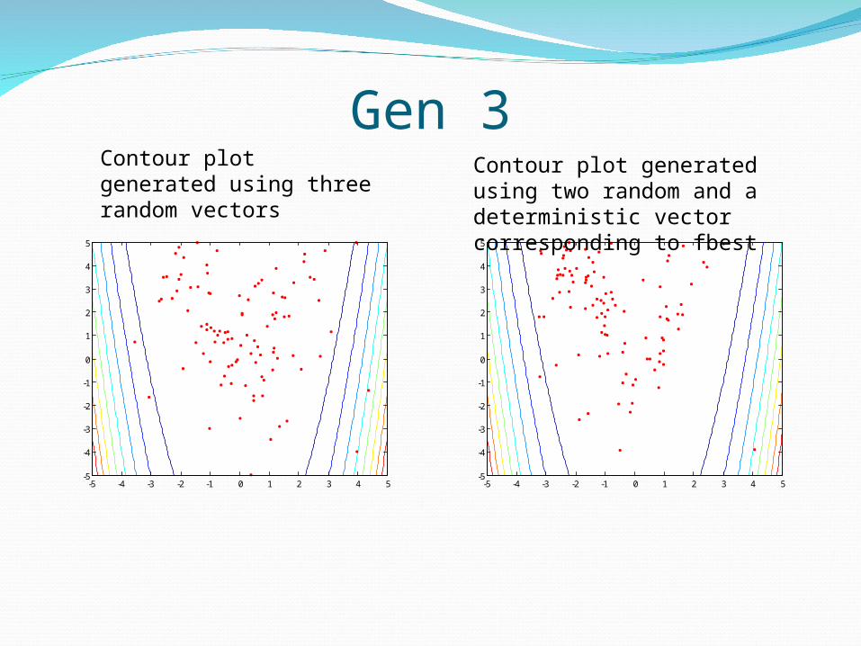
Gen 3

-5 -4 -3 -2 -1 0 1 2 3 4 5-5

-4

-3

-2

-1

0

1

2

3

4

5

-5 -4 -3 -2 -1 0 1 2 3 4 5-5

-4

-3

-2

-1

0

1

2

3

4

5



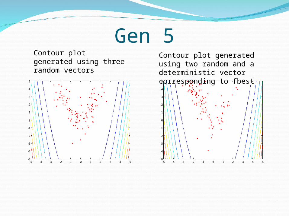
Gen 5

-5 -4 -3 -2 -1 0 1 2 3 4 5-5

-4

-3

-2

-1

0

1

2

3

4

5

-5 -4 -3 -2 -1 0 1 2 3 4 5-5

-4

-3

-2

-1

0

1

2

3

4

5



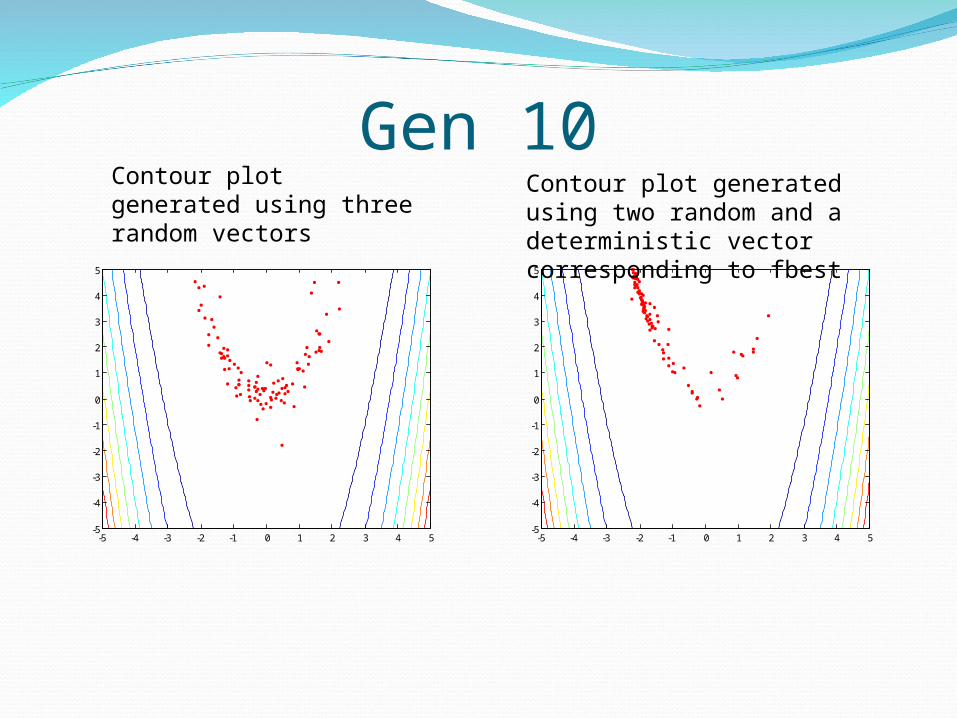
Gen 10

-5 -4 -3 -2 -1 0 1 2 3 4 5-5

-4

-3

-2

-1

0

1

2

3

4

5

-5 -4 -3 -2 -1 0 1 2 3 4 5-5

-4

-3

-2

-1

0

1

2

3

4

5



Gen 20

-5 -4 -3 -2 -1 0 1 2 3 4 5-5

-4

-3

-2

-1

0

1

2

3

4

5

-5 -4 -3 -2 -1 0 1 2 3 4 5-5

-4

-3

-2

-1

0

1

2

3

4

5



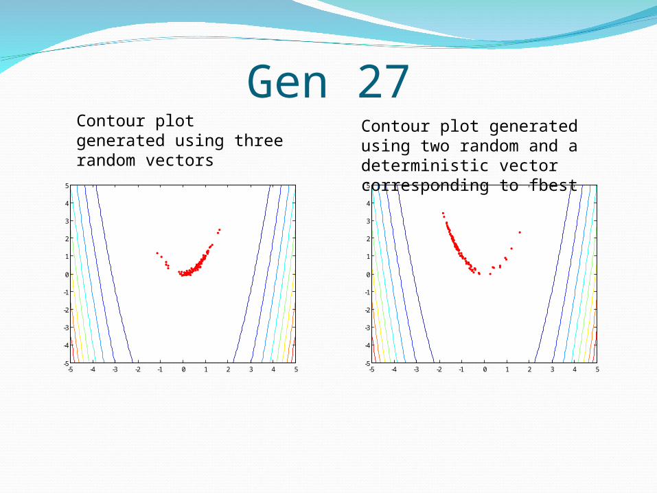
Gen 27

-5 -4 -3 -2 -1 0 1 2 3 4 5-5

-4

-3

-2

-1

0

1

2

3

4

5

-5 -4 -3 -2 -1 0 1 2 3 4 5-5

-4

-3

-2

-1

0

1

2

3

4

5



Gen 40

-5 -4 -3 -2 -1 0 1 2 3 4 5-5

-4

-3

-2

-1

0

1

2

3

4

5

-5 -4 -3 -2 -1 0 1 2 3 4 5-5

-4

-3

-2

-1

0

1

2

3

4

5



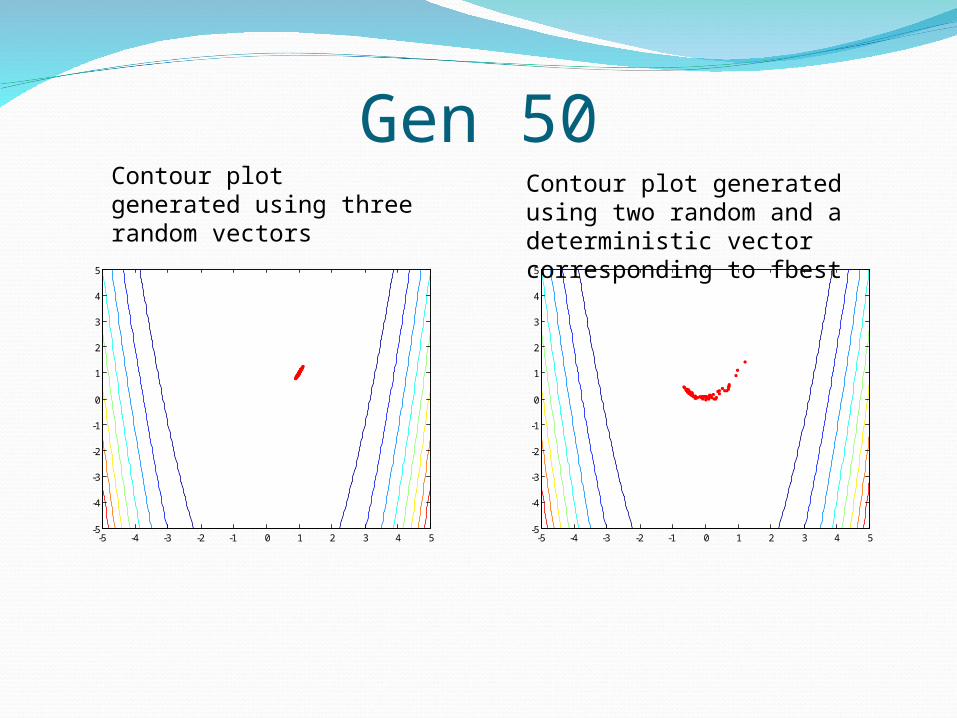
Gen 50

-5 -4 -3 -2 -1 0 1 2 3 4 5-5

-4

-3

-2

-1

0

1

2

3

4

5

-5 -4 -3 -2 -1 0 1 2 3 4 5-5

-4

-3

-2

-1

0

1

2

3

4

5



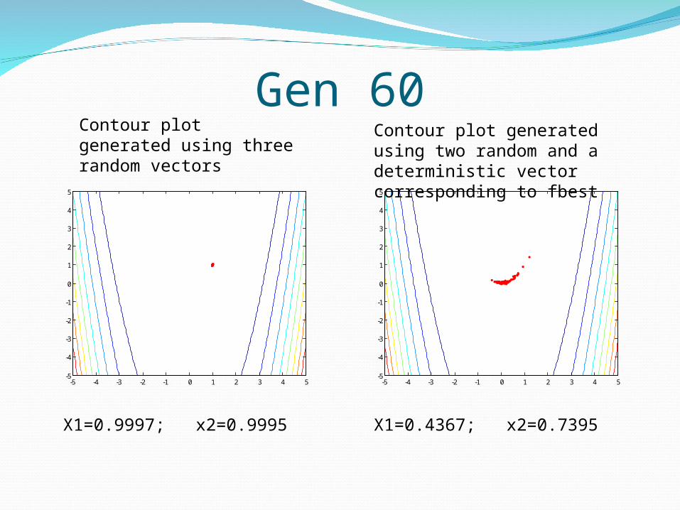
Gen 60

-5 -4 -3 -2 -1 0 1 2 3 4 5-5

-4

-3

-2

-1

0

1

2

3

4

5

-5 -4 -3 -2 -1 0 1 2 3 4 5-5

-4

-3

-2

-1

0

1

2

3

4

5

X1=0.9997; x2=0.9995 X1=0.4367; x2=0.7395



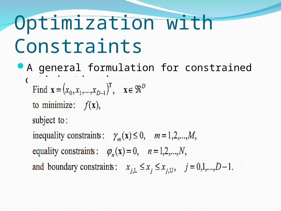
Optimization with ConstraintsA general formulation for constrained

optimization is

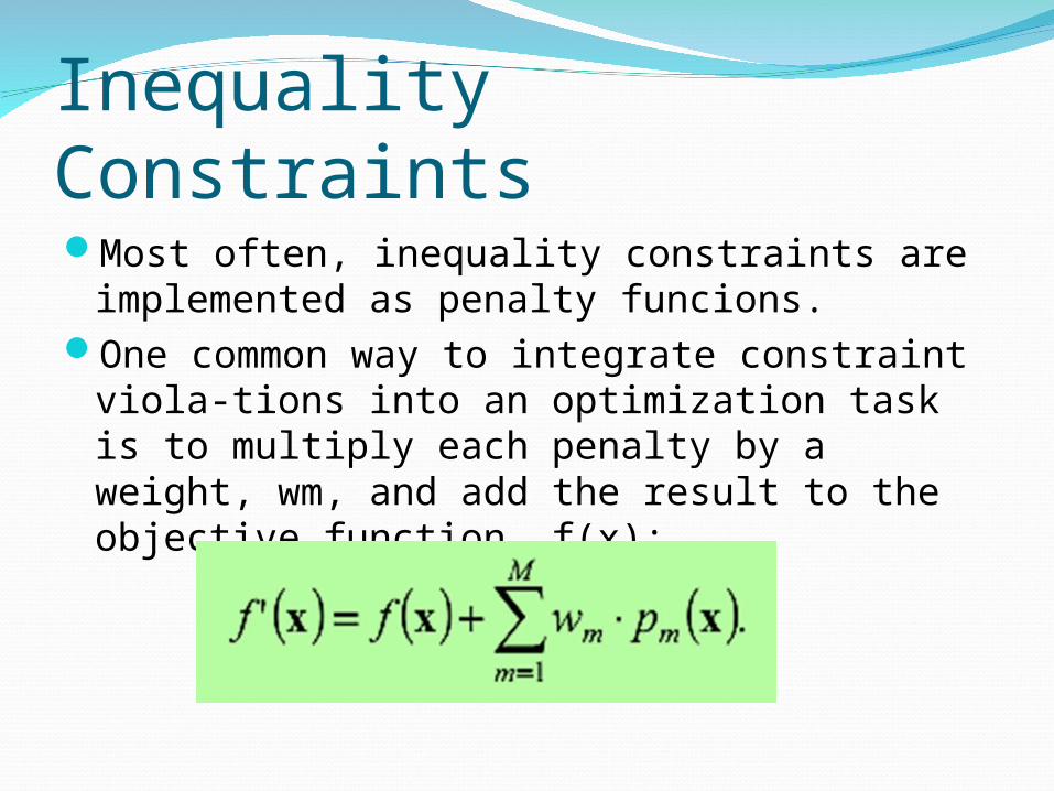
Inequality ConstraintsMost often, inequality constraints are

implemented as penalty funcions.One common way to integrate constraint

viola-tions into an optimization task is to multiply each penalty by a weight, wm, and add the result to the objective function, f(x):

Importance of adding weightsWeights help normalize all penalties to the same

range. Without normalization, penalty function

contributions may differ by many orders of magnitude, leaving violations with small penalties underrepresented until those that generate large penalties become just as small.

When there are many constraints, the main drawback of the penalty approach is that pre-specified weights must be well chosen to keep the population from converging upon either infeasible or non-optimal vectors.

Drawbacks of Penalty functionsSchemes that sum penalty functions run the risk

that one penalty will dominate unless weights are correctly adjusted. In addition, the population can converge upon an infeasible region if its objective function values are much lower than those in feasible regions. It can even happen that no set of weights will work. Because weight selection tends to be a trial and error optimization problem in its own right, simpler direct constraint handling methods have been designed that do not require the user to “tune” penalty weights.

Direct Constraint HandlingIn simple terms, Lampinen’s criterion selects

the trial vector ui,g if: 1.ui,g satisfies all constraints and has a lower

or equal objective function value than xi,g, or 2.ui,g is feasible and xi,g is not, or 3.ui,g and xi,g are both infeasible, but ui,g does

not violate any constraint more than xi,g.

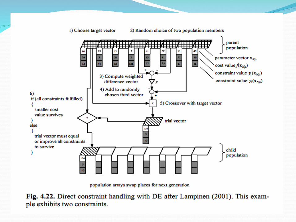
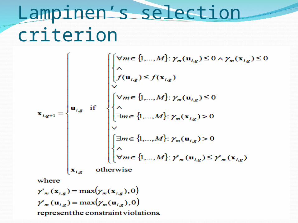
Lampinen’s selection criterion

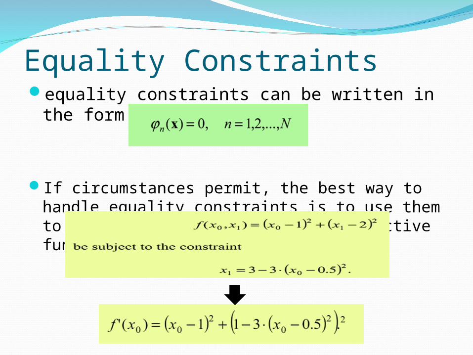
Equality Constraintsequality constraints can be written in the

form

If circumstances permit, the best way to handle equality constraints is to use them to eliminate variables from the objective function.

Eliminating variables ??Eliminating an objective function variable

with an equality constraint not only ensures that all vectors satisfy the constraint, but also reduces the problem’s dimension by 1.

In pactice, not all equality constraint equations can be solved for a term that also appears in the objective function. When it cannot be used to eliminate a variable, an equality constraint can be recast as a pair of inequality constraints.

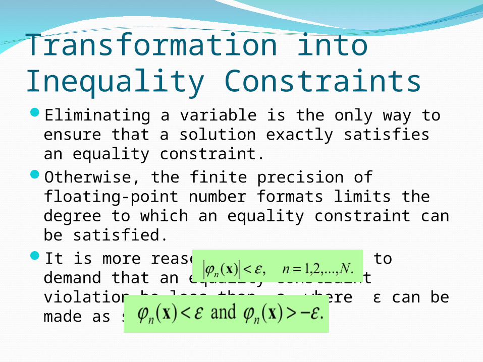
Transformation into Inequality ConstraintsEliminating a variable is the only way to ensure

that a solution exactly satisfies an equality constraint.

Otherwise, the finite precision of floating-point number formats limits the degree to which an equality constraint can be satisfied.

It is more reasonable, therefore, to demand that an equality constraint violation be less than ε, where ε can be made as small as desired:

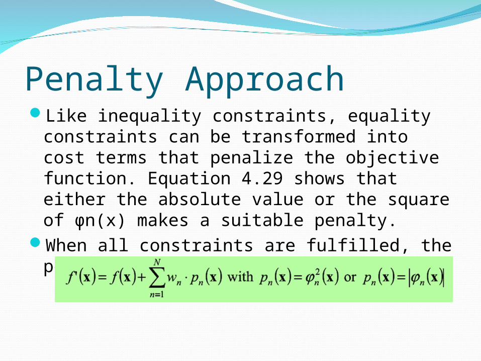
Penalty ApproachLike inequality constraints, equality

constraints can be transformed into cost terms that penalize the objective function. Equation 4.29 shows that either the absolute value or the square of ϕn(x) makes a suitable penalty.

When all constraints are fulfilled, the penalty term, like ε, becomes zero:

differential evolution

Documents