Computers & Operations Research 37 (2010) 509 -- 520

Contents lists available at ScienceDirect

Computers &Operations Research

journal homepage: www.e lsev ier .com/ locate /cor

Anovel hybrid discrete differential evolution algorithm for blocking flow shopscheduling problems

Ling Wanga, Quan-Ke Panb,∗, P.N. Suganthanc, Wen-HongWangb, Ya-Min Wangb

aTsinghua National Laboratory for Information Science and Technology (TNList), Department of Automation, Tsinghua University, Beijing 100084, ChinabCollege of Computer Science, Liaocheng University, Liaocheng 252059, PR ChinacSchool of Electrical and Electronic Engineering, Nanyang Technological University, 50 Nanyang Ave., 639798 Singapore, Singapore

A R T I C L E I N F O A B S T R A C T

Available online 24 December 2008

Keywords:Blocking flow shopDifferential evolutionDiscrete differential evolutionHybrid algorithmLocal searchSpeed-up

This paper proposes a novel hybrid discrete differential evolution (HDDE) algorithm for solving blockingflow shop scheduling problems to minimize the maximum completion time (i.e. makespan). Firstly, in thealgorithm, the individuals are represented as discrete job permutations, and new mutation and crossoveroperators are developed for this representation, so that the algorithm can directly work in the discretedomain. Secondly, a local search algorithm based on insert neighborhood structure is embedded in thealgorithm to balance the exploration and exploitation by enhancing the local searching ability. In addi-tion, a speed-up method to evaluate insert neighborhood is developed to improve the efficiency of thewhole algorithm. Computational simulations and comparisons based on the well-known benchmark in-stances of Taillard [Benchmarks for basic scheduling problems. European Journal of Operational Research1993;64:278–285], by treating them as blocking flow shop problem instances with makespan criterion,are provided. It is shown that the proposed HDDE algorithm not only generates better results than theexisting tabu search (TS) and TS with multi-moves (TS + M) approaches proposed by Grabowski andPempera [The permutation flow shop problem with blocking. A tabu search approach 2007;35:302–311],but also outperforms the hybrid differential evolution (HDE) algorithm developed by Qian et al. [Aneffective hybrid DE-based algorithm for multi-objective flow shop scheduling with limited buffers. Com-puters and operations research 2009;36(1):209–233] in terms of solution quality, robustness and searchefficiency. Ultimately, 112 out of 120 best known solutions provided by Grabowski and Pempera [Thepermutation flow shop problem with blocking. A tabu search approach 2007;35:302–311] and Ronconi[A branch-and-bound algorithm to minimize the makespan in a flowshop problem with blocking. Annalsof Operations Research 2005;138(1):53–65] are further improved by the proposed HDDE algorithm.

© 2009 Published by Elsevier Ltd.

1. Introduction

Flow shop scheduling problem is one of themost popularmachinescheduling problems with extensive engineering relevance, repre-senting nearly a quarter of manufacturing systems, assembly lines,and information service facilities in use nowadays [1–8]. This paperconsiders flow shop scheduling problems with blocking constraint.In blocking flow shops, there are no buffers between machines andhence intermediate queues of jobs waiting in the production systemfor their next operations are not allowed. Therefore, when needed,a job having completed processing on a machine has to remainon this machine and block itself until next machine is availablefor processing. The blocking flow shop scheduling problems have

∗ Corresponding author. Tel.: +866358238360; fax: +866358238809.E-mail address: qkpan@lcu.edu.cn (Q.-K. Pan).

0305-0548/$ - see front matter © 2009 Published by Elsevier Ltd.doi:10.1016/j.cor.2008.12.004

important applications in the production environment where pro-cessed jobs are sometimes kept in themachines because of the lack ofintermediate storage [9], or stock is not allowed in some stages of themanufacturing process because of technological requirements [10].On the other hand, it has been proved that the blocking flow shopscheduling problem to minimize makespan with three machines isNP-hard in the strong sense [11]. Therefore, it is of significance bothin theory and in engineering applications to develop effective andefficient novel solution procedures to solve such problems.

However, blocking flow shop scheduling problems have not cap-tured enough research so far [2,12]. Among the research, McCormichet al. [13] developed a constructive heuristic, known as profile fit-ting (PF), for solving sequencing problems in an assembly line withblocking to minimize cycle time. In their heuristic, the authors cre-ated a partial sequence by adding an unscheduled job to obtain theminimum sum of idle times and blocking times on machines. A morecomprehensive approach is presented by Leisten [14] for dealing

510 L. Wang et al. / Computers & Operations Research 37 (2010) 509 -- 520

with permutation and non-permutation flow shops with finite andunlimited buffers to maximize the use of buffers and to minimize themachine blocking. However, the author concluded that the heuris-tic did not produce better solutions than the Nawaz–Enscore–Ham(NEH) [16] heuristic. Ronconi [9] proposed three constructive heuris-tics, called minmax (MM), combination of MM and NEH (MME), andcombination of PF and NEH (PFE), respectively, for blocking flowshop problems with makespan criterion. It was demonstrated by theauthors that the MME and PFE heuristics outperformed the NEH al-gorithm in problems with up to 500 jobs and 20 machines. Based onthe connection between no-wait flow shop scheduling problems andflow shop scheduling problems with blocking, Abadi et al. [17] pro-posed a heuristic for minimizing cycle time in blocking flow shops.Recently, Ronconi and Henriques [12] studied the minimization ofthe total tardiness in flow shops with blocking scheduling and pre-sented some constructive heuristics. By computational tests, the au-thors showed that their new approaches were promising for theproblems considered.

With the development of computer technology, a few meta-heuristics have been used to solve blocking flow shop schedulingproblems. Caraffa [18] developed a genetic algorithmic approach forsolving large size restricted slowdown flow shop problems in whichblocking flow shop problems were special cases. Ronconi [4] pro-posed a heuristic algorithm based on branch-and-bound method byusing the new lower bounds which exploited the blocking natureand were better than those presented in their earlier paper [15]. Byapplying some properties of the problems associated with the blocksof jobs as well as using multi-moves to accelerate the convergenceto more promising areas of the solutions space, recently, Grabowskiand Pempera [2] developed two tabu search (TS) and TS with multi-move (TS+M) approaches. Computational results demonstrated thatthe TS and TS + M algorithms outperformed both the genetic algo-rithm [18] and Ronconi's method [4].

The differential evolution (DE) algorithm was first introducedby Storn and Price [19] to optimize complex continuous nonlin-ear functions. As a population-based evolutionary algorithm, theDE uses simple mutation and crossover operators to generate newcandidate solutions, and applies one-to-one competition schemeto greedily decide whether the new candidate or its parent willsurvive in the next generation. Due to its simplicity, ease of im-plementation, fast convergence, and robustness, the DE algorithmhas gained much attention and a wide range of successful applica-tions such as digital PID controller design [20], feed-forward neuralnetworks training [21,35], digital filter design [22] and earthquakehypocenter location [23]. However, because of its continuous na-ture, applications of the DE algorithm on scheduling problems arestill considerably limited [24–31]. Therefore, in this paper, we pro-pose a hybrid discrete DE (HDDE) algorithm for solving blockingflow shop scheduling problems with makespan criterion. In theproposed DDE algorithm, individuals are represented as discretejob permutations, and novel job-permutation-based mutation andcrossover operators are employed to generate new candidate so-lutions, and an effective insert-neighborhood-based local searchis embedded to enhance exploitation. Furthermore, a speed-upmethod for insert neighborhood structure is developed to reducecomputational time requirements. Simulation results and compar-isons demonstrate the effectiveness of the proposed HDDE algorithmin solving blocking flow shop scheduling problems with makespancriterion.

This paper is organized as follows. In Section 2, the blocking flowshop scheduling problem is stated and formulated. In Section 3, thespeed-up method for the insert neighborhood structure is proposed.In Section 4, the discrete DE (DDE) algorithm is proposed in detail.Section 5 presents a HDDE algorithm after explaining an effective lo-cal search. The computational results and comparisons are provided

1

1

1

1

2

2

2

2

3

3

3

3

e3,4

e3,1

t

m1

m2

m3

m4

e3,0

Fig. 1. Computation of ej,k .

in Section 6. Finally, we conclude the paper with some concludingremarks in Section 7.

2. The blocking flow shop scheduling problem

The blocking flow shop scheduling problem can be defined as fol-lows. There are n jobs from the set J = {1, 2, . . . ,n} and m machinesfrom the set M = {1, 2, . . . ,m}. Each job j ∈ J will be sequentially pro-cessed on machine 1, 2, . . . ,m. Operation oj,k corresponds to the pro-cessing of job j ∈ J on machine k (k = 1, 2, . . . ,m) during an uninter-rupted processing time pj,k, where its setup time is included into theprocessing time. At any time, each machine can process at most onejob and each job can be processed on at most one machine. The se-quence in which the jobs are to be processed is the same for eachmachine. Since the flow shop has no intermediate buffers, a job can-not leave a machine until its next machine downstream is free. Inother words, the job has to be blocked on its machine if its next ma-chine is not free. The aim is then to find a sequence for processingall jobs on all machines so that its maximum completion time (i.e.makespan) is minimized.

2.1. Mathematical model

Let a job permutation � = {�1,�2, . . . ,�n} represent the scheduleof jobs to be processed, and ej,k be the departure time of operationoj,k (illustrated in Fig. 1). According to the literature [9], ej,k can becalculated as follows

e1,0 = 0, (1)

e1,k = e1,k−1 + p1,k, k = 1, . . . ,m − 1, (2)

ej,0 = ej−1,1, j = 2, . . . ,n, (3)

ej,k = max{ej,k−1 + pj,k, ej−1,k+1}, j = 2, . . . ,n, k = 1, . . . ,m − 1, (4)

ej,m = ej,m−1 + pj,m, j = 1, . . . ,n, (5)

where ej,0, j=1, . . . ,n, denotes the starting time of job �j on the firstmachine. In the above recursion, the departure times of the firstjob on every machine are calculated first, then the second job, andso on until the last job. Then the makespan of the job permutation� = {�1,�2, . . . ,�n} is given by Cmax(�) = en,m, and its computationalcomplexity is O(mn).

Let fj,k be the tail, i.e., duration between the latest loading time ofoperation oj,k (k = m, . . . , 1) and the end of the operations, and fj,m+1be the duration between the latest completion time of operation oj,mand the end of the operations (illustrated in Fig. 2). To follow theblocking constraints, we can obtain the recursion below

fn,m+1 = 0, (6)

L. Wang et al. / Computers & Operations Research 37 (2010) 509 -- 520 511

fn,k = fn,k+1 + pn,k, k = m, . . . , 2, (7)

fj,m+1 = fj+1,m, j = n − 1, . . . , 1, (8)

fj,k = max(fj,k+1 + pj,k, fj+1,k−1), j = n − 1, . . . , 1, k = m, . . . , 2, (9)

fj,1 = fj,2 + pj,1, j = n, . . . , 1. (10)

In the above recursion, the tails of the last job on every machineare calculated first, then the second last job, and so on until the firstjob. Then, an alternative approach to calculate the makespan of jobpermutation �={�1,�2, . . . ,�n} can be given by Cmax(�)= f1,1 in timeO(mn).

Therefore, the objective of the blocking flow shop schedulingproblem with makespan criterion is to find a permutation �∗ in theset of all permutations � such that

Cmax(�∗)�Cmax(�), ∀� ∈ �. (11)

2.2. Graph representation

A graph representation model is used by Grabowski and Pem-pera [2] to present the blocking flow shop scheduling problem (seeFig. 3). For a permutation �, a graph G(�) = (Z,A) is created with aset of nodes Z = ⋃n

j=1⋃m

k=1(j, k) and a set of arcs A = A+ ∪ A0 ∪ A−,where the node (j, k) with weight p�j ,k represents the processing of

1

1

1

1

2

2

2

2

3

3

3

3

f1,4

t

m1

m2

m3

m4

f1,5

f1,1

Fig. 2. Computation of fj,k .

1 2

1

3 5 61

2

3

4

5

6

Machine/Job Block Anti-block

4 7 8

Fig. 3. A graph model blocking flow shop scheduling problem [2].

operation O�j ,k, and A+ = ⋃nj=1

⋃m−1k=1 {((j, k), (j, k + 1))} is a subset of

the arcs connecting consecutive operations of the same job, andA0 = ⋃n−1

j=1⋃m

k=1{((j, k), (j + 1, k))} is a subset of the arcs connectingoperations on the same machine in the processing order given by �,and A−=⋃n−1

j=1⋃m−1

k=1 {((j, k+1), (j+1, k))} is a subset of arcs associatedwith the blocking constraints, and each arc ((j, k+1), (j+1, k)) fromA− has weight −p�j ,k+1. The makespan Cmax(�) is equal to the longest(critical) path from node (1, 1) to node (n,m) in the graph G(�), whichcan be decomposed into several specific sub-paths and each of themcontains the nodes linked with the same type of arcs. The first typeof sub-paths is determined by the arcs in A0 which correspond tosequences of operations processed on the same machine withoutinserted idle time. The second type of sub-paths is defined by thearcs in A− which correspond to blocked jobs. For simplicity, denotethe first type of sub-paths and the second type of sub-paths as blocksand anti-blocks, respectively. Note that the critical path can containmany different blocks and anti-blocks, and all the blocks and anti-blocks are connected in series. A simple graph model is shown inFig. 3 for the blocking flow shop scheduling problem with n= 8 andm=6, where arcs from A+ and A0 are represented by solid lines, andarcs from A− by dashed lines, and nodes in the critical path by boldcircles.

3. Insert-neighborhood-based speed-up method

Insert neighborhood of a job permutation � = {�1,�2, . . . ,�n} iswidely used for flow shop scheduling problems in the literature [32],and is defined by considering all possible insert moves in the setV = {v(i, q)|i, q ∈ {1, 2, . . . ,n} ∧ q /∈ {i, i − 1}}. The insert move v(i, q)generates a permutation �′ from the permutation � by removing ajob �i from its original position i and inserting it into another positionq (q /∈ {i, i − 1}):

�′ = {�1, . . . ,�i−1, �i+1, . . . ,�i, �q, �q+1, . . . ,�n} if (i<q), (12)

�′ = {�1, . . . ,�q−1, �i, �q+1, . . . ,�i−1, �i+1, . . . ,�n} if (i>q). (13)

The number of neighbors in the insert neighborhood of a per-mutation � is (n− 1)2, so the computational complexity to evaluatethe whole insert neighborhood is O(mn3) by using each approachproposed in Section 2.1. However, making use of the similarity ofthe permutation � and its neighbor �′, and inspired by reduction of

512 L. Wang et al. / Computers & Operations Research 37 (2010) 509 -- 520

1

1

1

1

2

2

2

2

3

3

3

3

e'4,4

e'4,1

t

m1

m2

m3

m4

0

0

0

0

4

4

4

4

5

5

5

5

f4,1

f4,4

Fig. 4. Computation of makespan after inserting job 0 into position 4.

computational complexity presented by Grabowki [10], Taillard [33]and Smutnicki [34], we develop a speed-up to evaluate the insertneighborhood for the problems considered here. The procedure isgiven below:

Step 1: Calculate the departure times ej,k, j=1, 2, . . . ,n, k=1, 2, . . . ,musing Eqs. (1)–(5).

Step 2: Calculate the tails fj,k, j = n,n − 1, . . . , 1, k = m,m − 1, . . . , 1using Eqs. (6)–(10).

Step 3: Let i = 1.Step 4: Let �′′ = {�′′

1,�′′2, . . . ,�

′′n−1} be a partial permutation gener-

ated by removing job �i from the permutation �.Step 5: Get the departure times e′′

j,k, j=1, 2, . . . ,n−1, k=1, 2, . . . ,m,for the partial permutation �′′ as follows. If j< i, then let e′′

j,k = ej,k;else calculate e′′

j,k using Eqs. (1)–(5).Step 6: Get the tails f ′′

j,k, j = n − 1,n − 2, . . . , 1, k = m,m − 1, . . . , 1,for the permutation �′′ as follows. If j> i, then let f ′′

j,k = fj+1,k; elsecalculate f ′′

j,k using Eqs. (6)–(10).Step 7: Repeat the following steps until all possible positions q,

q ∈ {1, 2, . . . ,n} ∧ q /∈ {i, i − 1}, of the permutation �′′ are considered.Step 7.1: Insert job �i into position q and generates a permutation

�′.Step 7.2: Calculate the departure times e′

q,k by using the obtaineddeparture time e′′

q−1,k, where k = 1, 2, . . . ,m.Step 7.3: The makespan of the permutation �′ is given as follows

(illustrated in Fig. 4):

Cmax(�′) = mmaxk=1

(e′q,k + f ′′

q,k).

Step 8: Let i = i + 1. If i>n then stop; otherwise go back toStep 4.

There are n iterations for Steps 5–7, and each of these steps canbe executed in time O(mn). So, the computational complexity of thisspeed-up method is O(mn2) to evaluate the whole insert neighbor-hood of the permutation �.

In addition, according to the block properties presented byGrabowski [2,10,34] based on the graph model, we can further re-duce the computational time to evaluate an insert neighborhood.The theorem is given as follows:

Theorem 1 (Grabowski [2]). Let � ∈ � be any permutation with blocksBgi ,hi = (�gi ,�gi+1, . . . ,�hi ), (gi,hi) ∈ GH = {(gi,hi)|i = 1, . . . , lB} and anti-blocks Asi ,ti = (�si ,�si+1, . . . ,�ti ) (si, ti) ∈ ST = {(si, ti)|i = 1, . . . , lA}. Ifthe permutation �′ has been obtained by an interchange of jobs thatCmax(�′)<Cmax(�), then in �′

(1) at least one job �j ∈ Bgi ,hi precedes job �gi , for some (gi,hi) ∈ GH, or(2) at least one job �j ∈ Bgi ,hi succeeds job �hi , for some (gi,hi) ∈ GH, or(3) at least one job �j ∈ Asi ,ti precedes job �si , for some (si, ti) ∈ ST , or(4) at least one job �j ∈ Asi ,ti succeeds job �ti , for some (si, ti) ∈ ST.

It is concluded from the above theorem that some insert movescannot produce the permutations with better makespan. Since inour algorithm, we aim to find a better permutation than � in itsneighborhood, we will remove these non-improving moves from theinsert move set V to further save computational time. The procedureis given as follows:

Step 1: Set j = 1 and k = m.Step 2: If ej,k + fj+1,k = Cmax(�), then the following two cases may

ariseCase 1: ej,k = ej,k−1 + pj,k. In this case, let

Bk ={ {oj,k, oj+1,k} if Bk = { },Bk ∪ {oj+1,k} otherwise,

where Bk is a block.Case 2: ej,k >ej,k−1 + pj,k. In this case, let

ABk ={ {oj,k+1, oj+1,k} if ABk+1 = { },ABk+1 ∪ {oj+1,k} otherwise,

and

ABk+1 = { },

where ABk is an anti-block. If k= 1, then remove the non-improvingmoves from V according to anti-block ABk and Theorem 1, and letABk = { }.

Step 3: If ej,k + fj+1,k <Cmax(�), then remove the invalid movesfrom V according to theorem 1, Bk and ABk+1, then let Bk = { } andABk+1 = { }.

Step 4: If k>0, let k = k − 1 and go to Step 2.Step 5: If j<n, let j= j+1 and k=m, then go to Step 2; otherwise

stop the procedure.The above method can effectively extract some non-improving

insert moves from the set V, so the neighbors of the permutation � tobe evaluated are tailed off and the computational time requirementto find the better neighbors is further decreased. It is easy to verifythat in some special cases, such as all pj,k are identical and n�3,each machine has single block containing all jobs. After executingthe procedure, the remaining moves in the set V is decreased to4n− 8, whereas the initial number of moves is no less than (n− 1)2.Note that when the non-improving moves are extracted, the indicesof the neighbors will be changed.

4. DDE algorithm

4.1. Brief introduction to DE algorithm

The basic DE algorithm [19] is one of the latest population-basedand stochastic global optimizers. It adopts a floating-point encod-ing scheme and takes advantage of the differentiation informationamong the population to find the global optimum in the continuous

L. Wang et al. / Computers & Operations Research 37 (2010) 509 -- 520 513

search space. Starting from a random initialization of PS target in-dividuals, it creates PS new candidate solutions by mutation andcrossover operators, and then applies selection operator to deter-mine the new target individuals in the next generation. Let Xt

i =�xti1, xti2, . . . , xtin, Vt

i =�vti1,vti2, . . . ,vtin and Uti =�uti1,uti2, . . . ,utin denote

the ith target individual, the ith mutant individual, and the ith trialindividual at iteration t, respectively. Following the DE/rand/1/binscheme [19], the procedure of the basic DE algorithm can be de-scribed as follows:

Step 1: Initialization phase. Set the parameters and generate apopulation of PS individuals randomly. Let bestsofar be the best in-dividual found so far, and t = 0.

Step 2: Mutation phase. Set t = t + 1, and generate mutant indi-vidual Vt

i , i = 1, 2, . . . , PS, as follows:

vtij = xt−1aj + Z × (xt−1

bj − xt−1cj ), (14)

where a, b and c are three random integers in the range [1, PS] suchthat a, b, c and i are pairwise different, and j = 1, 2, . . . ,n, and Z ∈(0, 2) is a scale factor to control the amplification of the differentialvariation between two target individuals.

Step 3: Crossover phase. Generate trial individual Uti , i=1, 2, . . . , PS,

as follows:

utij ={vtij if rand( )<CR or j = Dj,

xt−1ij otherwise,

(15)

where CR ∈ [0, 1] is a crossover parameter to control the diversity ofthe population, rand( ) denotes a uniform random number between0 and 1, and Dj refers to an index randomly chosen from the set{1, 2, . . . ,n} to ensure that at least one dimension of Ut

i is differentfrom its counterpart Xt−1

i .Step 4: Selection phase. For a minimization problem, each new

target individual can be generated as follows:

Xti =

{Uti if f (Ut

i )� f (Xt−1i ),

Xt−1i otherwise,

(16)

where f (·) is the objective function.Step 5: Update bestsofar.Step 6: If a stopping criterion is satisfied, then output bestsofar;

otherwise go back to Step 2.

4.2. DDE algorithm

The basic DE algorithm cannot be used to directly generate dis-crete job permutations since it is originally designed to solve contin-uous optimization problems where the individuals are representedby floating-point numbers. Therefore, in this section, we will presenta novel DDE algorithm to solve the blocking flow shop schedulingproblem after explaining solution representation, new mutation andcrossover operators, and initialization.

4.2.1. Solution representationThe job-permutation-based representation has been widely used

in the literature for flow shop scheduling problems and it is easy todecode to reduce the cost of the algorithm [6]. In this section, weadopt this representation and an example is given in Table 1.

4.2.2. Job-permutation-based mutation operatorAccording to the basic DE algorithm, a mutant individual is gen-

erated by adding the weighted difference between two target in-dividuals randomly selected from previous population to anotherindividual, so a job-permutation-based mutation operator can be

presented as follows:

Vti = Xt−1

a ⊕ Z ⊗ (Xt−1b − Xt−1

c ), (17)

where a, b and c are three random integers in the range [1, PS] suchthat a, b, c and i are pairwise different, and i = 1, 2, . . . , PS, and Z ∈[0, 1] is a mutant scale factor.

The above formula consists of two components. The first compo-nent refers to the weighted difference between two target individ-uals Xt−1

b and Xt−1c , that is,

�ti = Z ⊗ (Xt−1

b − Xt−1c )

⇔ �ti,j =

{xt−1b,j − xt−1

c,j if rand( )<Z,0 otherwise,

(18)

where �ti = (�t

i,0,�ti,1, . . . ,�

ti,n) is a temporary vector.

The second component is to produce a mutant individual Vti by

adding �ti to another target individual Xt−1

a , that is,

Vti = Xt−1

a ⊕ �ti

⇔ vtij = xt−1aj ⊕ �t

ij = mod((xt−1aj + �t

ij + n),n), (19)

where “mod” denotes the modulus operator whose result is the re-mainder when the first operand is divided by the second. This oper-ator ensures that each dimension of Vt

i can represent a job. In orderto better understand the proposed mutation operator, an example isgiven in Fig. 5.

From Fig. 5, it follows that each dimension of Vti represents a

job, but Vti itself cannot always represent a complete sequence since

some jobs may repeat many times whereas other jobs may be lost.However, from the crossover operator of the basic DE algorithm, itcan be seen that a mutant individual is used to enhance perturbationto a target individual to avoid premature convergence to a non-globallocal optimum. Therefore, it is not necessary to ensure a feasiblesolution by mutation operator, and a legal target individual can beobtained by the following crossover operator.

4.2.3. Job-permutation-based crossover operatorThe crossover operator generates a trial individual Ut

i by com-bining a mutant individual Vt

i and a target individual Xt−1i , and we

expect the Uti to be better than Xt−1

i . To well inherit good structuresfrom the target individual Xt−1

i and to yield a better Uti , the job-

permutation-based crossover operator is given as follows (illustratedby an example in Fig. 6):

Step 1: From j = 1 to n, remove job vti,j ∈ Vti if rand( )�CR or the

job has already been in Vi.Step 2: Let Ut

i = Xt−1i , and eliminate the jobs included in Vi from

Uti .Step 3: The first job from Vi is taken and inserted in the best

position of Uti by evaluating all the possible slots of Ut

i . This step isrepeated until Vi is empty. Now a complete schedule is obtained.

4.2.4. Population initializationSince NEH heuristic [16] is one of the well-know heuristics in

the literature, and it performs better than PF approach developed byMccormick et al. [13] and the heuristics by Leistein [14] for the con-sidered problem, to guarantee an initial population with a certainquality and diversity, we take advantage of NEH to produce an in-dividual, while the other individuals are randomly generated in thesolution space. The NEH heuristic has two phases. In phase I, jobs areordered in descending sums of their processing times. In phase II, ajob sequence is established by evaluating the partial schedules basedon the initial order of phase I. In this paper, the speed-up methodproposed in Section 3 is used to evaluate the partial schedules, sothe NEH heuristic can be executed in time O(mn2) for the blockingflow shop scheduling problem.

514 L. Wang et al. / Computers & Operations Research 37 (2010) 509 -- 520

Table 1An example of the job-permutation-based representation.

Dimension j 1 2 3 4 5 6 7xi,j 3 4 6 2 5 0 1Job permutation 3 4 6 2 5 0 1

0 1 2 3 4 5Xb

2 0 5 3 1 4Xc

-2 1 -3 0 3 1Xb-Xc

0.2 0.6 0.4 0.5 0.1 0.7rand()

-2 1 -3 0 3 1Xb-Xc

Δi -2 0 -3 0 3 0

1 0 5 3 2 4Xc

Δi -2 0 -3 0 3 0

Vi = Xa Δi 5 0 2 3 5 4

Fig. 5. Mutation operator: (a) Xb − Xc; (b) �i = Z ⊗ (Xa − Xb) with Z = 0.5 and (c)Vti = Xt−1

a ⊕ �ti .

4.2.5. Procedure of the DDE algorithmBased on the above design, the procedure of the DDE algorithm

for solving the blocking flow shop scheduling problem is presentedas follows:

Step 1: Initialization phase. Set the parameters PS, CR, and Z. Ini-tialize population. Let bestsofar be the best individual found so far,and t = 0.

Step 2: Mutation phase. Set t = t + 1, and generate PS mutantindividuals by using the job-permutation-based mutation operator.

Step 3: Crossover phase. Generate PS trial individuals by using thejob-permutation-based crossover operator.

Step 4: Selection phase. Decide PS target individuals for next gen-eration.

Step 5: Update bestsofar.Step 6: If a stopping criterion is satisfied, then output bestsofar;

otherwise go back to Step 2.

Vi 5 0 2 3 5 4

Xi 1 0 5 3 24

Vi

rand()

Vi

Ui

Ui 1 0 3 4

Ui 1 0 3

5 2Vi

Insert

Ui 1 5 0 3

4

4

2Vi

Insert

1 5 0 3

Ui 1 5 0 3 2

4

4

5 0 2 3 5 4

0.3 0.7 0.2 0.5 0.2 0.5

5 2

1 0 5 3 24

Fig. 6. Crossover operator: (a) Vi and Xi; (b) remove jobs from Vi (CR = 0.5); (c) letUi = Xi and remove the jobs included in Vi from Ui and (d) obtain Ui by insertingjobs of Vi to the best position of Ui .

Unlike the basic DE algorithm, the DDE algorithm adoptsthe job-permutation-based encoding scheme, employs the job-permutation-based mutation and crossover operators, and takesadvantage of the initialization based on NEH heuristic, so itcan be easily applied to the blocking flow shop schedulingproblem.

L. Wang et al. / Computers & Operations Research 37 (2010) 509 -- 520 515

5. HDDE algorithm

5.1. A problem-dependent local search

To balance the exploration and exploitation, a problem-dependent local search is presented and applied to each trial indi-vidual Ut

i with a probability Pl to enhance the local searching ability.That is, a uniform random number between 0 and 1 is firstly gener-ated, and the individual will undergo the local search if the randomnumber is less than Pl. For the job-permutation-based optimizationproblems, insert, swap, and inverse operators are commonly usedto produce a neighboring solution [2]. Among them, insert operatoris the most suitable for performing a fine local search [28]. Thus,we employ insert operator to be embedded in the DDE algorithm torefine local search for the problem considered. The procedure of thelocal search is described as follows:

Step 1: Let i = 0, j = 0, and produce a reference sequence �r ={�r

1,�r2, . . . ,�

rn} randomly.

Step 2: Let i = i + 1, and set i = i − n if i>n.Step 3: Extract job �r

i from the trial individual sequence Uti , and

insert it into all the other possible slots of Uti , respectively. Denote

the best obtained sequence as �b.Step 4: If f (�b)<f (Ut

i ), then let Uti =�b and j=0; otherwise, j=j+1.

Step 5: If j�n, then go back to step 2; otherwise stop the proce-dure.

The above local search algorithm is effective and efficient due tothe following reasons. Firstly, the local search is performed to thetrial individual Ut

i but not the target individual Xti , so the algorithm

can avoid both cycling search and getting trapped in a non-globallocal optimum. Secondly, in the local search, the incumbent solutionis updated only when a better solution is found, so the algorithm canrapidly reach a local solution. Lastly, by using the speed-up methodproposed in Section 3, the insert neighbors can be evaluated effi-ciently. Thus, the local search algorithm tends to enhance the localexploitation of the DDE algorithm in a relatively short time.

5.2. The HDDE algorithm

Based on the DDE algorithm and the local search presented inSection 5.1, the basic procedure of the HDDE algorithm is given asfollows:

Step 1: Initialization phase. Set the parameters PS, CR, Z, and Pl.Initialize population. Let bestsofar be the best individual found so far,and t = 0.

Step 2: Mutation phase. Set t = t + 1, and generate PS mutantindividuals by using the job-permutation-based mutation operator.

Step 3: Crossover phase. Generate PS trial individuals by using thejob-permutation-based crossover operator.

Step 4: Local search phase. Perform the local search to Uti , i =

1, 2, . . . , PS, with probability Pl.Step 5: Selection phase. Select PS target individuals by one-to-one

selection operator for next generation.Step 6: Update bestsofar.Step 7: If a stopping criterion is satisfied, then stop the procedure

and output bestsofar; otherwise go back to Step 2.It can be seen that the HDDE algorithm not only applies the DDE-

based evolutionary searching mechanism to effectively perform ex-ploration for promising solutions within the whole solution space,but it also employs the problem-dependent local search to performexploitation for solution improvement in the local neighborhoods.Since both the balance of exploration and exploitation and efficiencyof solution evaluation are stressed, it is expected to achieve good re-sults for the blocking flow shop scheduling problems with makespancriterion.

6. Computational results

6.1. Experimental setup

To test the performance of the proposed DDE/HDDE algorithm, acomprehensive experimental evaluation and comparison with otherpowerful methods are presented based on the well-known flow shopbenchmark set of Taillard [1]. The benchmark set is composed of12 subsets of given problems with the size ranging from 20 jobsand five machines to 500 jobs and 20 machines, and each subsetconsists of ten instances. We treat them as the blocking flow shopscheduling problems with makespan criterion. And, in our test, theproposed DDE/HDDE algorithm is coded in C + + and the exper-iments are executed on a Pentium P-IV 3.0GHz PC with 512MBmemory. The parameters are set as follows: F = 0.2, CR = 0.2, PS =20, Pl = 0.2, and the maximum computational time is set as T =5mnms. Each instance is run 10 independent replications and in eachreplication we compute the percentage relative difference (PRD) asfollows:

PRD = 100 × (CRon − CA)CRon

, (20)

where CRon is the referenced makespan provided by Ronconi [4], andCA is the makespan found by the DDE/HDDE algorithm. Furthermore,average percentage relative difference (APRD), maximum percentagerelative difference (MaxPRD), minimum percentage relative differ-ence (MinPRD), and the standard deviation (SD) of PRD are calculatedas the performance statistics.

6.2. Comparison of the DDE/HDDE and DE/HDE algorithms

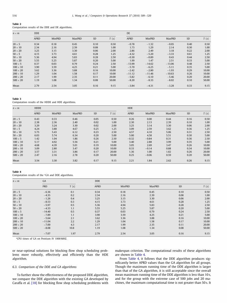
Recently, an effective HDE-based algorithm was developed byQian et al. [3] for solving multi-objective flow shop scheduling prob-lems with limited buffers between consecutive machines. In the HDEalgorithm, a largest-order-value rule was employed to convert thecontinuous values of individuals to discrete job permutations, and avery efficient local search algorithm was incorporated to emphasizeexploitation. By the experimental simulations based on the well-known benchmark instances collected from OR library, the authorsdemonstrated the effectiveness and efficiency of their HDE algo-rithm. In this paper, we modify the HDE algorithm for the blockingflow shop scheduling problem and code it in C+ +. The parametersof the HDE algorithm is consistent with those in [3], and the max-imum computation time is also set as T = 5mnms. Computationalsimulations are carried out on the same PC as mentioned before onthe same benchmarks. For each instance, 10 independent replica-tions are also conducted to obtain statistics. The computational re-sults produced by the DE (the HDE algorithm without local search)and HDE algorithms are reported in Tables 2 and 3, respectively.

It can be seen from Table 2 for the same computational time,the overall mean APRD and SD values yielded by the DDE algorithmare equal to 2.79% and 0.16%, respectively, which are much betterthan those (−3.84% and 0.33%) generated by the DE algorithm. Moreimportantly, the DDE algorithm produced substantially better PRDvalues with smaller SD values than the DE algorithm for all theproblem sizes and all instances as well. From these observations, itis concluded that the DDE algorithm is more robust, effective andefficient than the DE algorithm for blocking flow shop schedulingproblems.

The results reported in Table 3 indicate that the HDDE algo-rithm generates significantly better APRD values with smaller SDvalues than the HDE algorithm for each problem size using thesame computational time. As the problem size increases, the supe-riority of the HDDE algorithm over the HDE algorithm increases.Thus, it is concluded that the HDDE algorithm can reach optimal

516 L. Wang et al. / Computers & Operations Research 37 (2010) 509 -- 520

Table 2Computation results of the DDE and DE algorithms.

n × m DDE DE

APRD MinPRD MaxPRD SD T (s) APRD MinPRD MaxPRD SD T (s)

20 × 5 0.34 0.18 0.45 0.10 0.50 −0.78 −1.32 −0.05 0.40 0.5020 × 10 2.34 2.16 2.39 0.08 1.00 1.73 1.29 2.14 0.30 1.0020 × 20 3.25 3.15 3.30 0.06 2.00 2.86 2.49 3.18 0.22 2.0050 × 5 4.15 3.73 4.61 0.28 1.25 −4.32 −5.20 −3.33 0.61 1.2550 × 10 5.36 4.94 5.83 0.28 2.50 −0.30 −0.89 0.43 0.44 2.5050 × 20 5.55 5.25 5.87 0.20 5.00 1.99 1.47 2.51 0.33 5.00100 × 5 0.37 0.03 0.79 0.24 2.50 −13.99 −14.62 −13.06 0.48 2.50100 × 10 3.90 3.59 4.25 0.21 5.00 −5.70 −6.25 −5.11 0.35 5.00100 × 20 3.62 3.36 3.88 0.16 10.00 −2.42 −2.80 −1.93 0.29 10.00200 × 10 1.29 1.04 1.58 0.17 10.00 −11.12 −11.46 −10.63 0.26 10.00200 × 20 2.17 1.99 2.35 0.11 20.00 −5.82 −6.10 −5.46 0.20 20.00500 × 20 1.19 1.08 1.34 0.08 50.00 −8.20 −8.33 −8.02 0.10 50.00

Mean 2.79 2.54 3.05 0.16 9.15 −3.84 −4.31 −3.28 0.33 9.15

Table 3Computation results of the HDDE and HDE algorithms.

n × m HDDE HDE

APRD MinPRD MaxPRD SD T (s) APRD MinPRD MaxPRD SD T (s)

20 × 5 0.43 0.33 0.46 0.05 0.50 0.26 0.00 0.44 0.16 0.5020 × 10 2.38 2.36 2.40 0.02 1.00 2.30 2.13 2.39 0.10 1.0020 × 20 3.29 3.24 3.30 0.02 2.00 3.25 3.14 3.30 0.06 2.0050 × 5 4.24 3.88 4.67 0.25 1.25 3.09 2.59 3.62 0.36 1.2550 × 10 5.75 5.43 6.12 0.23 2.50 4.57 4.10 5.06 0.31 2.5050 × 20 6.03 5.74 6.34 0.20 5.00 5.00 4.58 5.51 0.30 5.00100 × 5 1.42 1.04 1.86 0.26 2.50 −0.32 −0.84 0.31 0.36 2.50100 × 10 5.17 4.92 5.56 0.21 5.00 3.40 2.88 3.99 0.35 5.00100 × 20 4.68 4.39 5.01 0.19 10.00 3.05 2.69 3.47 0.26 10.00200 × 10 3.09 2.80 3.47 0.20 10.00 0.33 −0.14 0.88 0.34 10.00200 × 20 3.57 3.31 3.86 0.17 20.00 1.36 1.00 1.82 0.26 20.00500 × 20 2.47 2.16 2.78 0.20 50.00 0.25 −0.06 0.59 0.20 50.00

Mean 3.54 3.30 3.82 0.17 9.15 2.21 1.84 2.62 0.26 9.15

Table 4Computation results of the aGA and DDE algorithms.

n × m GA DDE

PRD T (s) APRD MinPRD MaxPRD SD T (s)

20 × 5 −6.36 0.1 0.34 0.18 0.45 0.10 0.5020 × 10 −4.35 0.2 2.34 2.16 2.39 0.08 1.0020 × 20 −1.26 0.4 3.25 3.15 3.30 0.06 2.0050 × 5 −8.53 0.3 4.15 3.73 4.61 0.28 1.2550 × 10 −5.97 0.5 5.36 4.94 5.83 0.28 2.5050 × 20 −4.33 1.1 5.55 5.25 5.87 0.20 5.00100 × 5 −14.40 0.5 0.37 0.03 0.79 0.24 2.50100 × 10 −7.89 1.1 3.90 3.59 4.25 0.21 5.00100 × 20 −5.64 2.1 3.62 3.36 3.88 0.16 10.00200 × 10 −11.04 2.2 1.29 1.04 1.58 0.17 10.00200 × 20 −7.00 4.3 2.17 1.99 2.35 0.11 20.00500 × 20 −8.08 10.8 1.19 1.08 1.34 0.08 50.00

Mean −7.07 1.97 2.79 2.54 3.05 0.16 9.15

aCPU times of GA on Pentium IV 1000MHZ.

or near-optimal solutions for blocking flow shop scheduling prob-lems more robustly, effectively and efficiently than the HDEalgorithm.

6.3. Comparison of the DDE and GA algorithms

To further show the effectiveness of the proposed DDE algorithm,we compare the DDE algorithm with the existing GA developed byCaraffa et al. [18] for blocking flow shop scheduling problems with

makespan criterion. The computational results of these algorithmsare shown in Table 4.

From Table 4, it follows that the DDE algorithm produces sig-nificantly better APRD values than the GA algorithm for all groups.Though the maximum running time of the DDE algorithm is largerthan that of the GA algorithm, it is still acceptable since the overallmean maximum running time of the DDE algorithm is less than 10 s,and for the group with the extreme case of 500 jobs and 20 ma-chines, the maximum computational time is not greater than 50 s. It

L. Wang et al. / Computers & Operations Research 37 (2010) 509 -- 520 517

Table 5Computation resultsa of the TS, TS + M and HDDE algorithms.

n × m TS TS + M HDDE

PRD T(s) PRD T (s) APRD MinPRD MaxPRD SD T (s)

20 × 5 −1.64 2.4 −0.34 2.7 0.43 0.33 0.46 0.05 0.5020 × 10 1.45 4.1 1.76 4.6 2.38 2.36 2.40 0.02 1.0020 × 20 2.88 7.1 2.94 7.6 3.29 3.24 3.30 0.02 2.0050 × 5 −0.55 6.0 0.55 6.2 4.24 3.88 4.67 0.25 1.2550 × 10 1.98 10.6 3.52 10.8 5.75 5.43 6.12 0.23 2.5050 × 20 3.68 19.0 4.26 19.3 6.03 5.74 6.34 0.20 5.00100 × 5 −3.03 12.2 −2.62 12.4 1.42 1.04 1.86 0.26 2.50100 × 10 1.71 21.9 2.66 22.1 5.17 4.92 5.56 0.21 5.00100 × 20 2.01 39.2 3.03 39.4 4.68 4.39 5.01 0.19 10.00200 × 10 −0.60 44.1 0.58 44.3 3.09 2.80 3.47 0.20 10.00200 × 20 1.24 79.2 2.31 79.4 3.57 3.31 3.86 0.17 20.00500 × 20 0.63 207 1.47 209 2.47 2.16 2.78 0.20 50.00

Mean 0.81 37.73 1.68 38.15 3.54 3.30 3.82 0.17 9.15

aCPU times of TS and TS + M on Pentium IV 1000MHZ.

Table 6Upper bounds produced by the HDDE algorithm.

HDDE TS + M RON HDDE TS + M RON HDDE TS + M RON HDDE TS + M RON20 × 5 50 × 5 100 × 5 200 × 10

1374 1387 1384 3033 3163 3151 6291 6639 6455 13,756 14,220 14,1131408 1424 1411 3226 3348 3395 6136 6481 6214 13,621 14,089 14,1271280 1293 1294 3039 3173 3184 6063 6299 6124 13,741 14,149 14,4161448 1451 1448 3147 3277 3303 5839 6120 5976 13,718 14,156 14,4351341 1348 1366 3192 3338 3272 6065 6340 6173 13,721 14,130 14,1191363 1366 1363 3183 3330 3400 5971 6244 6094 13,474 13,963 13,9091381 1387 1381 3054 3168 3228 6095 6346 6262 13,925 14,386 14,5631379 1388 1384 3081 3228 3260 5985 6289 6061 13,863 14,256 14,3291373 1392 1378 2929 3068 3104 6234 6559 6474 13,659 13,954 13,923

1283 1302 1283 3146 3285 3264 6273 6509 6366 13,744 14,224 14,435

20 × 10 50 × 10 100 × 10 200 × 20

1698 1698 1736 3667 3776 3913 7131 7320 7496 15,057 15,334 15,5791833 1836 1897 3523 3641 3798 6816 7108 7281 15,284 15,522 15,7281659 1674 1677 3515 3588 3723 6956 7233 7400 15,360 15,713 15,9151535 1555 1622 3685 3786 3885 7261 7413 7670 15,276 15,687 16,0391617 1631 1658 3650 3745 3934 6913 7168 7317 15,183 15,443 15,9381590 1603 1640 3622 3747 3831 6739 6993 7301 15,223 15,472 15,9111622 1629 1634 3704 3778 3957 6874 7092 7247 15,296 15,522 15,8981731 1754 1741 3590 3708 3774 6940 7143 7315 15,310 15,540 16,0221747 1759 1777 3556 3668 3784 7133 7327 7631 15,243 15,394 15,817

1782 1782 1847 3642 3729 3928 7065 7299 7411 15,284 15,523 15,969

20 × 20 50 × 20 100 × 20 500 × 20

2436 2449 2530 4516 4627 4886 7891 8101 8347 37,172 37,860 38,3342234 2242 2297 4296 4411 4668 7931 8105 8372 37,485 38,044 38,6422479 2483 2560 4290 4388 4666 7935 8071 8265 37,209 37,732 38,1632348 2348 2399 4393 4479 4650 7930 8081 8365 37,291 38,062 38,6252435 2450 2538 4284 4359 4475 7944 8074 8304 37,232 37,991 38,4922383 2398 2467 4308 4372 4521 7971 8151 8450 37,513 38,132 38,5512390 2397 2502 4325 4402 4576 8051 8273 8507 37,121 37,561 38,1792328 2345 2411 4337 4444 4688 8102 8248 8584 37,202 37,750 38,6642363 2363 2421 4332 4423 4532 8007 8116 8341 37,116 37,730 38,339

2323 2334 2407 4439 4609 4846 8050 8261 8489 37,492 38,014 38,540

should be noted that when the maximum running time of the GA al-gorithm is increased to 475.0 s for the extreme case, it still producedthe much worse APRD value (−2.57) [2] than the DDE algorithm.Therefore, we can conclude that the DDE algorithm outperforms theGA algorithm on the considered problems.

6.4. Comparison of the HDDE and TS/TS + M algorithms

In this section, the HDDE algorithm is compared with two TS al-gorithms (TS and TS + M) [2] proposed by Grabowski and Pempera

who concluded that the TS and TS+M algorithm were the best per-forming algorithms when compare to GA developed by Caraffa et al.[18] and the heuristic presented by Ronconi [4]. The computationalresults of these algorithms are reported in Table 5.

From Table 5, it follows that the HDDE algorithm performs sig-nificantly better than both the TS and TS + M algorithms, since theoverall mean ARPD value yielded by the HDDE algorithm is equalto 3.54%, which is 4.37 and 2.11 times higher than those generatedby the TS (0.81%) and TS+M (1.68%) algorithms, respectively. Moreimportantly, the HDDE algorithm produces much better APRD value

518 L. Wang et al. / Computers & Operations Research 37 (2010) 509 -- 520

Table 7Comparison of the HDDE, DDE and MLS algorithms.

n × m HDDE MLS DDE

APRD MinPRD MaxPRD SD T (s) APRD MinPRD MaxPRD SD T (s) APRD MinPRD MaxPRD SD T (s)

20 × 5 0.43 0.33 0.46 0.05 0.50 −0.86 −1.60 −0.09 0.49 0.50 0.34 0.18 0.45 0.10 0.5020 × 10 2.38 2.36 2.40 0.02 1.00 1.23 0.60 1.93 0.41 1.00 2.34 2.16 2.39 0.08 1.0020 × 20 3.29 3.24 3.30 0.02 2.00 2.47 1.95 3.04 0.36 2.00 3.25 3.15 3.30 0.06 2.0050 × 5 4.24 3.88 4.67 0.25 1.25 1.62 0.97 2.25 0.41 1.25 4.15 3.73 4.61 0.28 1.2550 × 10 5.75 5.43 6.12 0.23 2.50 3.10 2.34 3.87 0.48 2.50 5.36 4.94 5.83 0.28 2.5050 × 20 6.03 5.74 6.34 0.20 5.00 3.86 3.23 4.65 0.44 5.00 5.55 5.25 5.87 0.20 5.00100 × 5 1.42 1.04 1.86 0.26 2.50 −0.70 −1.28 −0.12 0.38 2.50 0.37 0.03 0.79 0.24 2.50100 × 10 5.17 4.92 5.56 0.21 5.00 3.06 2.49 3.69 0.38 5.00 3.90 3.59 4.25 0.21 5.00100 × 20 4.68 4.39 5.01 0.19 10.00 2.77 2.39 3.17 0.25 10.00 3.62 3.36 3.88 0.16 10.00200 × 10 3.09 2.80 3.47 0.20 10.00 1.64 1.04 2.28 0.39 10.00 1.29 1.04 1.58 0.17 10.00200 × 20 3.57 3.31 3.86 0.17 20.00 2.29 1.88 2.79 0.28 20.00 2.17 1.99 2.35 0.11 20.00500 × 20 2.47 2.16 2.78 0.20 50.00 2.25 1.87 2.58 0.24 50.00 1.19 1.08 1.34 0.08 50.00

Mean 3.54 3.30 3.82 0.17 9.15 1.89 1.32 2.50 0.38 9.15 2.79 2.54 3.05 0.16 9.15

0 500 1000 1500 2000 2500 3000 3500 4000 4500 50007100

7200

7300

7400

7500

7600

7700

mak

espa

n

running time

MLS

DDEHDDE

Fig. 7. Convergence rate cure of the MLS, DDE and HDDE algorithms for problem ta 81.

than both the TS and TS + M algorithms for all problem size and allinstances as well. Even the MinPRD value produced by the HDDEalgorithm is much better than the PRD value by the TS and TS + Malgorithms. Especially, the HDDE algorithm is far superior to the TSand TS + M algorithms for problem sizes of 50 × 5 and 100 × 5. Interms of the computational time requirements, although the com-puter for the HDDE algorithm is about three times faster than theone used by Grabowski and Pempera [2], the average computationtime of the HDDE algorithm is shorter than one third of that of boththe TS and TS+M algorithms for each instances. It highlights the factthat the HDDE algorithm performed significantly better than the TSand TS+M algorithms. In addition, the mean SD value resulting fromthe HDDE algorithm is very small, demonstrating the robustness ofthe HDDE algorithm to the initialization.

Table 6 reports the makespan found by the HDDE algorithm. Itshould be noted that for 112 out of 120 instances, the HDDE algo-rithm has found better makespan values (highlighted in bold) thanboth the TS+M [2] and Ron's algorithms (here denoted as Ron) [4].All these results confirm the favorable performance of the proposed

HDDE algorithm over the TS and TS+M algorithms in terms of aver-age percent relative deviation value and computational time as well.Hence, we can concluded that the HDDE algorithm is more effec-tive and efficient than both the TS and TS+M algorithms for solvingblocking flow shop scheduling problems with makespan criterion.

6.5. Effectiveness of combining the DDE and local search algorithms

The computational experiments and comparisons are conductedbetween the HDDE algorithm with the DDE and multi-start randomlocal search (denoted as MLS) algorithms to show the effectivenessof combining the DDE-based global search and problem-dependentlocal search. The MLS algorithm is presented by removing the DDE-based search from the HDDE algorithm, and its parameters are setas follows: PS= 20, Pl = 0.2. The computational results are shown inTable 7.

It is easily observed from Table 7 that the HDDE algorithm is thewinner since the results generated by the HDDE algorithm are signif-icantly better than those by the DDE and MLS algorithms. To better

L. Wang et al. / Computers & Operations Research 37 (2010) 509 -- 520 519

0 0.1 0.2 0.3 0.4 0.5 0.6 0.7 0.8 0.9 10

0.5

1

1.5

2

2.5

3

3.5

4

4.5

5APRD

PRD

MinPRDMaxPRDSD

Parameter Pl

Fig. 8. Effect of the parameter Pl .

understand the performance of the HDDE algorithm, the typical con-vergence rate curves for these three algorithms based on benchmarkinstance ta 81 are shown in Fig. 7. It can be easily seen from Fig. 7that the HDDE algorithm converges much faster to reach lower lev-els than both the DDE and MLS algorithms. The conclusion is similarfor other benchmark instances.

Based on the above comparisons, it is concluded that the HDDEalgorithm is superior to the DDE and MLS algorithms in terms ofsolution quality, robustness and convergence rate for the blockingflow shop scheduling problems with makespan criterion. This couldbe explained by the fact that in the HDDE algorithm, the DDE algo-rithm generates good start points for the local search algorithm byperforming global exploration, while the local search algorithm fur-ther refines the obtained solutions by performing local exploitation,and guides the DDE algorithm to more promising search area. Thatis to say, the superiority in terms of searching quality and robust-ness of the HDDE algorithm should be attributed to the combinationof global search and local search, i.e., the balance of exploration andexploitation.

6.6. Effect of the parameter Pl

Clearly, Pl is a key parameter for the HDDE algorithm. Hence,we further investigate the effect of Pl on solution quality. We set Plfrom 0.05 to 1.0 with a step equal to 0.05 and fix other parameters.The similar computational experiments are conducted. The statisticalresults are presented in Fig. 8.

From Fig. 8, it follows that as Pl increases, the APRD value pro-duced by the HDDE algorithm varies within a very small range. Thissuggested that Pl does not affect the searching quality of the HDDEalgorithm too much. In other words, the HDDE algorithm is robustin regard to the parameter Pl.

7. Conclusions

By applying a job-permutation-based representation, a noveljob-permutation-based mutation and crossover operators, and aproblem-dependent local search, we first propose a novel hybriddiscrete differential evolution (HDDE) algorithm for solving block-

ing flow shop scheduling problems with makespan criterion. Due tothe effective hybridization of the differential-evolution-based globalsearch and insert-neighborhood-based local search, the global ex-ploration and local exploitation of the HDDE algorithm are wellbalanced. Furthermore, the efficiency of the HDDE algorithm isstressed by using a speed-up method to evaluate whole insertionneighborhood. Simulation results and comparisons demonstratedthe superiority of the proposed HDDE algorithm in terms of so-lution quality, robustness and effectiveness. The future work is toapply the HDDE algorithm to other kinds of combinatorial opti-mization problems and develop multi-objective HDDE algorithmsfor multi-objective scheduling problems.

Acknowledgments

This research is partially supported by National Science Foun-dation of China under Grants 60874075, 70871065, 60834004,60774082, National 863 Hi-Tech RandD Plan under Grant2007AA04Z155, and Open Research Foundation from State KeyLaboratory of Digital Manufacturing Equipment and Technology(Huazhong University of Science and Technology), the Project-sponsored by SRF for ROCS, SEM, and Postdoctoral Science Founda-tion of China under Grants 20070410791. QKP and PNS acknowledgethe financial support offered by the A*Star (Agency for Science,Technology and Research, Singapore) under Grant #052 101 0020.

References

[1] Taillard E. Benchmarks for basic scheduling problems. European Journal ofOperational Research 1993;64:278–85.

[2] Grabowski J, Pempera J. The permutation flow shop problem with blocking. Atabu search approach 2007;35:302–11.

[3] Qian B, Wang L, Huang DX, Wang WL, Wang X. An effective hybrid DE-based algorithm for multi-objective flow shop scheduling with limited buffers.Computers and operations research 2009;36(1):209–33.

[4] Ronconi DP. A branch-and-bound algorithm to minimize the makespan in aflowshop problem with blocking. Annals of Operations Research 2005;138(1):53–65.

[5] Pinedo M. Scheduling: theory, algorithms and systems. NJ: Prentice-Hall; 2002.[6] Wang L, Zheng DZ. An effective hybrid heuristic for flow shop scheduling.

International Journal of Advanced Manufacturing Technology 2003;21:38–44.[7] Pan Q-K, Wang L. No-idle permutation flow shop scheduling based on a

hybrid discrete particle swarm optimization algorithm. International Journal ofAdvanced Manufacturing Technology 2008;39:796–807.

520 L. Wang et al. / Computers & Operations Research 37 (2010) 509 -- 520

[8] Pan Q-K, Tasgetiren MF, Liang Y-C. A discrete particle swarm optimizationalgorithm for the no-wait flowshop scheduling problem. Computers andOperations Research 2008;35(9):2807–39.

[9] Ronconi DP. A note on constructive heuristics for the flowshop problem withblocking. International Journal of Production Economics 2004;87:39–48.

[10] Grabowski J, Pempera J. Sequencing of jobs in some production system.European Journal of Operational Research 2000;125:535–50.

[11] Hall NG, Sriskandarajah C. A survey of machine scheduling problems withblocking and no-wait in process. Operations Research 1996;44:510–25.

[12] Tonconi DP, Henriques LRS. Some heuristic algorithms for total tardinessminimization in a flowshop with blocking. OMEGA—International Journal ofManagement Science 2009;37(2):272–81.

[13] McCormich ST, Pinedo ML, Shenker S, Wolf B. Sequencing in an assembly linewith blocking to minimize cycle time. Operations Research 1989;37:925–36.

[14] Leisten R. Flowshop sequencing problems with limited buffer storage.International Journal of Production Research 1990;28:2085–100.

[15] Ronconi DP, Armentano VA. Lower bounding schemes for flowshops withblocking in-process. Journal of the Operational Research Society 2001;52:1289–97.

[16] Nawaz M, Enscore EEJ, Ham I. A heuristic algorithm for the m-machine, n-jobflow shop sequencing problem. OMEGA—International Journal of ManagementScience 1983;11:91–5.

[17] Abadi INK, Hall NG, Sriskandarajh C. Minimizing cycle time in a blockingflowshop. Operations Research 2000;48:177–80.

[18] Caraffa V, Ianes S, Bagchi TP, Sriskandarajah C. Minimizing makespan in ablocking flowshop using genetic algorithms. International Journal of ProductionEconomics 2001;70:101–15.

[19] Storn R, Price K. Differential evolution—a simple and efficient adaptive schemefor global optimization over continuous spaces. Journal of Global Optimization1997;11:341–59.

[20] Chang FP, Hwang C. Design of digital PID controllers for continuous-time plantswith integral performance criteria. Journal of the Chinese Institute of ChemicalEngineers 2004;35:683–96.

[21] Ilonen J, Kamarainen JK, Lampinen J. Differential evolution training algorithmfor feed-forward neural networks. Neural Process Letters 2003;17:93–105.

[22] Storn R. Designing digital filters with differential evolution. In: Corne D, DorigoM, Glover F, editors. New ideas in optimization. London, UK: McGraw-Hill;1999.

[23] Ruzek B, Kvasnicka M. Differential evolution in the earthquake hypocenterlocation. Pure and Applied Geophysics 2001;158:667–93.

[24] Qian B, Wang L, Hu R. et al. A hybrid differential evolution for permutation flow-shop scheduling. International Journal of Advanced Manufacturing Technology2008;38(7–8):757–77.

[25] Onwubolu GC, Davendra D. Scheduling flow shops using differentialevolution algorithm. European Journal of Operational Research 2006;171(2):674–92.

[26] Tasgetiren MF, Pan QK, Suganthan PN, Liang YC. A discrete differential evolutionalgorithm for the no-wait flowshop problem with total flowtime criterion. In:Proceedings of the 2007 IEEE symposium on computational intelligence inscheduling. p. 251–8.

[27] Tasgetiren MF, Sevkli M, Liang YC. et al. A particle swarm optimization anddifferential algorithm for job shop scheduling problem. International Journal ofOperations Research 2006;3:120–35.

[28] Qian B, Wang L, Huang DX, Wang X. An effective hybrid DE-based algorithm forflow shop scheduling with limited buffers. International Journal of ProductionResearch 2009;36(1):209–33.

[29] Pan Q-K, Wang L. A novel differential evolution algorithm for the no-idlepermutation flow shop scheduling problems. European Journal of IndustrialEngineering 2008;2(3):279–97.

[30] Pan Q-K, Tasgetiren MF, Liang Y-C. A discrete differential evolution algorithmfor the permutation flowshop scheduling problem. In: Proceedings of the Ninthannual conference on genetic and evolutionary computation, London, England;2007. p. 126–33.

[31] Tasgetiren MF, Pan Q-K, Liang Y-C. A discrete particle swarm optimizationalgorithm for the generalized traveling salesman problem. In: Proceedings ofthe ninth annual conference on genetic and evolutionary computation, London,England; 2007. p. 158–67.

[32] Grabowski J, Pempera J. Some local search algorithms for no-wait flow-shop problem with makespan criterion. Computers and Operations Research2005;32:2197–212.

[33] Taillard E. Some efficient heuristic methods for the flow shop sequencingproblems. European Journal of Operational Research 1990;47:65–74.

[34] Smutncki C. A two-machine permutation flow shop scheduling problem withbuffers. OR Spectrum; 1998.

[35] Zhu Q-Y, Qin AK, Suganthan PN, Huang G-B. Evolutionary extreme learningmachine. Pattern Recognition 2005;38(10):1759–63.