differential geometry of the möbius space i - hu …sulanke/diffgeo/moebius/mdg.pdf · r. sulanke...
TRANSCRIPT
R. Sulanke
Differential Geometry of theMöbius Space I
Curve Theory
March 5, 2012
Manuscript


V
CopyrightThis msnuscript, the accompanying Mathematica Notebooks and packagesare public. Authors who intend to publish a changed or completed version ofthem should do it under their own names with the condition that they cite theoriginal item with the internet address or other source where they got it. I amnot responsible for errors or damages originated by the use of the procedurescontained in my notebooks or packages; everybody who applies them shouldtest carefully whether they are appropriate for his purposes.

Preface
The manuscript presented here is the first part of a planned book about thedifferential geometry of submanifolds of the Möbius space. It is devoted tocurve theory, developed systematically using E. Cartan’s method of movingframes [4]. In our papers R. Sulanke, A. Švec [29], see also [25], we describedan interpretation of E. Cartan’s method, and we wanted to test our work in ahomogeneous space in which invariant linear connections don’t exist and themethods of Riemannian geometry can not be applied directly. Appropriatesuch spaces are the n-dimensional Möbius spaces, whose geometry coincideswith the conformal geometry of the n-spheres Sn. The advantage of Möbiusgeometry is not only that it is very near to Euclidean geometry and admitsclear graphic illustrations of the geometric objects in low dimensions, but alsothat it contains the classical Riemannian geometries of constant curvature assubgeometries, what allows metric interpretations of the conformal invariants.
There exist important very interesting monographs containing Möbius dif-ferential geometry. The earliest I know is the monograph [3] of W. Blaschkeand G. Thomsen which appeared in 1929. It is a very rich collection of mat-ters about the geometry of circles and spheres presenting much more thanMöbius geometry; it contains also the Laguerre and Lie geometries. A mul-tilateral and very attractive presentation of the recent developement of thesubject is contained in the monograph [10] of U. Hertrich-Jeromin. A verygeneral monograph about conformal structures is the book [1] of M. A. Akivisand V. V. Goldberg; in this book the method of G. F. Laptev is applied. Inspite of the rich material contained in these monographs they may not beconsidered as systematic presentations of Möbius differentiual geometry; forexample the differential geometry of curves in the 3-dimensional Möbius spaceis treated very incompletely in [3] as a serie of exercises, and not mentionedin the monographs [10] and [1]. The more modest aim of our book is to givea detailed description of the geometry of submanifolds of the n-dimensionalMöbius space emphasizing the manifolds of points and considering the familiesof subspheres as tools only. The presentation of the subject is as elementary as

II Preface
possible, applying the elements of the theory of Lie groups and homogeneousspaces.
The first chapter contains basic concepts of Möbius geometry, the Möbiusgroup, the simply connected space forms: the spherical, hyperbolical and Eu-clidean spaces embedded into the Möbius space, their isometry groups assubgroups of the Möbius group which is the conformal group of he standardn-sphere. The deciding object for the differential geometry of a homogeneousspace G/H is the structure form of the group G and the isotropy action of Hon it. We elaborate this concept for linear homogeneous spaces and considerthe special cases needed in our presentation of the Möbius geometry.
The second chapter starts with a description of E. Cartan’s method ofmoving frames. Section 2.1 may be read as a heuristic approach to this method;for a deeper understanding the study of the relevant literatur is necessary.For a reader who is mainly interested in a special geometry it can be saidthat a general understanding of the method suffices to apply it in a givensituation; any Lie group requires a special investigation guided by the generalmethod leading to interesting results which sometimes may be considered ascorollaries of general theorems but often need special proofs. Section 2.2 basedon a joined paper [23] with Ch. Schiemangk contains such a special applicationto immersions into the Möbius space. The there defined Möbius structure ofan m-dimensional immersion contains an invariant Riemannian metric on theimmersed manifold and an invariant linear connection of its normal bundle.The Möbius structure becomes singular at umbilical points. A criterion for animmersion to be a part of a subsphere is proved.
Chapter 3 is devoted to the Möbius geometry of curves, it is an elaborationof my paper [26]. For generally curved curves a natural parameter and acomplete system of invariants, its conformal curvatures, are found. A so-calledFundamental Theorem, stating the existence and uniqueness (up to Möbiustransformations) of a curve with given curvatures is proved. Curves containedin a subsphere are characterized by the vanishing of some higher curvatures. Insection 3.2 the curves of constant curvatures are treated; they are identified asorbits of 1-parametric subgroups of the Möbius group. In the last section someresults about curves in linear Lie groups and linear homogeneous spaces arecollected, forming the theoretical background of curve theory in homogeneousspaces.
Connected with this book some Mathematica notebooks about MöbiusGeometry are published on my homepage. There one find tools for the cal-culation of the moving frame and the invariants and the visualization of thecurves and surfaces treated in chapter 3. Moreover, a framework for workingin the geometry of the Möbius space and the spaces of constant curvatures isdeveloped.
In the forthcoming not yet written chapters the geometry of hypersurfases,particularly surfaces, and special problems of the Möbius differential geometrywill be considered as far as I am able to complete my program.
Grabow, November 16, 2010, Rolf Sulanke.

Contents
Preface . . . . . . . . . . . . . . . . . . . . . . . . . . . . . . . . . . . . . . . . . . . . . . . . . . . . . I
1 Möbius Space. Space Forms . . . . . . . . . . . . . . . . . . . . . . . . . . . . . . . 11.1 The Projective Model of the Möbius Space Sn . . . . . . . . . . . . . . 1
1.1.1 The Isotropy Group of the Möbius Space . . . . . . . . . . . . . 61.1.2 A Vector Model of the Möbius Space . . . . . . . . . . . . . . . . 7
1.2 Space Forms and their Isometry Groups. . . . . . . . . . . . . . . . . . . . 81.2.1 Simply Connected Space Forms En
c embedded in Sn . . . 81.2.2 Frame Bundles . . . . . . . . . . . . . . . . . . . . . . . . . . . . . . . . . . . . 10
1.3 Structure Forms . . . . . . . . . . . . . . . . . . . . . . . . . . . . . . . . . . . . . . . . . 131.3.1 Structure Forms of Linear Lie Groups . . . . . . . . . . . . . . . . 141.3.2 The Structure Form of the Möbius Group . . . . . . . . . . . . 191.3.3 Basis Forms . . . . . . . . . . . . . . . . . . . . . . . . . . . . . . . . . . . . . . 201.3.4 Lie Algebras . . . . . . . . . . . . . . . . . . . . . . . . . . . . . . . . . . . . . . 221.3.5 Linear Isotropy Representations . . . . . . . . . . . . . . . . . . . . . 271.3.6 Applications to Möbius Geometry . . . . . . . . . . . . . . . . . . . 291.3.7 Applications to the Space Forms En
c . . . . . . . . . . . . . . . . . 32
2 The Möbius Structure of an Immersion . . . . . . . . . . . . . . . . . . . . 352.1 E. Cartan’s Method of Moving Frames . . . . . . . . . . . . . . . . . . . . . 352.2 The Möbius Structure of an Immersion . . . . . . . . . . . . . . . . . . . . . 38
3 Möbius Geometry of Curves . . . . . . . . . . . . . . . . . . . . . . . . . . . . . . . 493.1 Fundamental Theorem for Curves in the Möbius Space Sn . . . . 503.2 Curves of Constant Curvatures . . . . . . . . . . . . . . . . . . . . . . . . . . . . 67
3.2.1 Curves of Constant Curvatures in S2 . . . . . . . . . . . . . . . . 683.2.2 Curves of Constant Curvatures in S3 . . . . . . . . . . . . . . . . 713.2.3 Historical Notes . . . . . . . . . . . . . . . . . . . . . . . . . . . . . . . . . . . 77
3.3 Curves in Linear Homogeneous spaces . . . . . . . . . . . . . . . . . . . . . . 783.3.1 Curves in Group Spaces . . . . . . . . . . . . . . . . . . . . . . . . . . . . 793.3.2 Curves in Linear Homogeneous Spaces . . . . . . . . . . . . . . . 83

IV Contents
References . . . . . . . . . . . . . . . . . . . . . . . . . . . . . . . . . . . . . . . . . . . . . . . . . . . . . 89
Index . . . . . . . . . . . . . . . . . . . . . . . . . . . . . . . . . . . . . . . . . . . . . . . . . . . . . . . . . . 91

1
Möbius Space. Space Forms
1.1 The Projective Model of the Möbius Space Sn
The Möbius space is defined to be the n-dimensional sphere Sn consideredas the non-degenerate quadric of index 1 in the (n+ 1)-dimensional real pro-jective space Pn+1. As usual we consider the real n + 1-dimensional pro-jective geometry as the geometry in the lattice of subspaces of an (n + 2)-dimensional real vector space V n+1. The points of the projective space Pn+1
are the 1-dimensional subspaces of V n+2, the k-dimensional projective sub-spaces, shortly named k-planes, are the (k + 1)-dimensional vector subspacesof V n+2. In the following we apply concepts, notations, and results of projec-tive and Möbius geometry as described in [19]. Sometimes the fact is confusingthat the same object, e. g. a vector subspace, is considered from the vecto-rial or the projective point of view leading to other dimensions: Denoting theusual dimension of a vector subspace by dim and the projective dimension byDim, one has
DimU = k ⇐⇒ dimU = k + 1.
This is valid also for the null space U = o; considered from the projectivepoint of view it is called the nopoint and denoted by o. If the k-planes areinterpreted as point sets, i. e. as the sets of its 1-dimensional subspaces of thevector space, the nopoint is the empty set. It has the projective dimensionDim o = −1.
Any point x ∈ Pn+1 can be represented by a basis vector x = o of thecorresponding 1-dimensional subspace of V n+2; we write x = [x], and generally[A] for the span of a set A ⊂ V . The vector coordinates xi of x with respectto a frame (bi) are the corresponding homogeneous coordinates of the point xwith respect to this frame; they are defined up to a common factor λ = 0.
All the non-degenerate n-dimensional quadrics of index 1 are projectivelyequivalent. We may fix an (n+ 2)-frame in the vector space V such that theequation of the quadric Sn in the corresponding homogeneous coordinates ofPn+1 has the normal form
2 1 Möbius Space. Space Forms
⟨x, x⟩ = −(x0)2 +n+1∑i=1
(xi)2 = 0. (1)
Here ⟨, ⟩ denotes the pseudo-orthogonal scalar product of index 1 in the real(n + 2)-dimensional vector space V = V n+2, which defines the projectivespace Pn+1, the vectors x ∈ V, x = o, solving (1) describe the isotropic coneJ ⊂ V n+2, whose generators represent the points of Sn, and
x =n+1∑j=0
ejxj = ejx
j (2)
is the basis representation of x with respect to the fixed pseudo-orthonormalframe (ej) of V , fulfilling
ϵij := ⟨ei, ej⟩ = ϵiδij , with ϵ0 = −1, ϵi = 1 for i = 1, . . . , n+ 1, (3)
δij the Kronecker symbol. As in (2) we will often use the sum conventionthat over the full range of indices appearing as subscripts and superscripts ofan expression is to summarize.
The m-dimensional subspheres Σm ⊂ Sn, m = 0, . . . , n, are defined asintersections
Σm = Sn ∩Am+1 ⊂ Sn
of Sn with projective (m + 1)-planes A, containing at least two points; such(m+ 1)-planes are called planes intersecting Sn. We speak about point pairsΣ0 = x, y ⊂ Sn × Sn, x = y, as 0-spheres, circles are 1-spheres, and hyper-spheres Σn−1 ⊂ Sn are subspheres of dimension n − 1. Since the subspheresΣm contain at least two points of Sn, the vector subspaces Wm+2 defining theintersecting projective m+1-planes Am+1 = Wm+2 ⊂ V contain at least twolinearely independent isotropic vectors; therefore they correspond bijectivelyto the pseudo-Euclidean vector subspaces Wm+2 of index 1 and dimensionm+ 2. They are m-dimensional Möbius spaces themselves.
The Möbius group M(n) is defined to be the group of all projective trans-formations of Pn+1 preserving Sn. In [19] the Möbius group is identified withthe pseudo-orthogonal group O(1, n + 1)+ of all linear transformations pre-serving the scalar product in the (n+2)-dimensional pseudo-Euclidean vectorspace V n+2 of index 1 and a time orientation of V . Indeed, we prove
Proposition 1. The Möbius group M(n), n ≥ 1, is isomorphic to the pseudo-orthogonal group O(1, n+ 1)+.
P r o o f. Clearly, each projective transformation f generated by a lineartransformation g ∈ O(1, n + 1)+ satisfies f(Sn) = Sn, see (1). On the otherhand, let the projective transformation f preserving Sn be generated by thelinear transformation g, and define
b(x, y) := ⟨gx, gy⟩.

1.1 The Projective Model of the Möbius Space Sn 3
Since f preserves Sn it follows
b(x, x) = 0 ⇐⇒ ⟨x, x⟩ = 0.
We consider a line [x+ ty] starting at a point x = [x] ∈ Sn in a non-isotropicdirection y, ⟨y, y⟩ = 0. A point of the line belongs to the sphere Sn if andonly if t = 0 or t = −2⟨x, y⟩/⟨y, y⟩. The same argument is valid for the scalarproduct replaced by the bilinear form b, and it follows
b(x, y)⟨y, y⟩ = ⟨x, y⟩b(y, y) if ⟨x, x⟩ = 0, ⟨y, y⟩ = 0.
We consider the pseudo-orthonormal basis (ei) of V n+2 satisfying (3) andevaluate the last equation for x = e0 + ei, i > 0, and y = e0. It follows
b(e0, ei) = 0 for i > 0.
Similarely, evaluating the equation for the same x and y = ej , j > 0, weconclude
b(ei, ej) = δijλj with λj := b(ej , ej).
Since e0 + ei for i > 0 is an isotropic vector we obtain
b(e0 + ei, e0 + ei) = λ0 + λi = 0 for i > 0.
Setting λ := λ1 and applying Sylvester’s theorem of inertia and n+ 2 ≥ 3 weconclude b(x, y) = λ⟨x, y⟩ with λ > 0. Since the projective transformation f canbe generated also by ±gλ−1/2 we may restrict to the linear transformationsg ∈ O(1, n+ 1)+. 2
Another proof of Proposition 1, valid for n ≥ 2 only, can be given bythe argument: Any projective transformation f preserving the hyperquadricSn maps hyperspheres, as intersections of Sn with hyperplanes, into hyper-spheres. By Proposition 2.7.3 in [19] the map f can be generated by a lineartransformation g ∈ O(1, n+ 1)+.
Möbius geometry is the geometry of the transitive transformation group[M(n), Sn], i.e. the geometry of the hypersphere under the action of theMöbius group. Möbius differential geometry is the theory of submanifoldsof Sn under the action of M(n). It is well known that M(n), n > 1, coincideswith the group of all conformal transformations of Sn provided with the Rie-mannian metric of constant curvature (induced by the standard embeddingof Sn as the hypersphere of radius 1 in the Euclidean space En+1), see e.g.U. Hertrich-Jeromin [10], § 1.5. Therefore, instead of Möbius geometry oneoften speaks about the conformal geometry of the hypersphere.
The scalar product defines a polarity F in the lattice of projective sub-spaces, corresponding to the orthogonality of the vector subspaces:
F : A 7−→ F (A) := A⊥.
The map F is an involutive bijection of the lattice inverting the order. Forthe dimensions it follows

4 1 Möbius Space. Space Forms
DimA = k ⇐⇒ DimA⊥ = n− k, (A ⊂ Pn+1). (4)
To each point x ∈ Pn+1 corresponds its polar x⊥, a hyperplane of Pn+1.The polars of points x ∈ Sn can be characterized as the hyperplanes in-tersecting Sn in a single point, namely x ∈ x⊥; this hyperplanes are calledtangent spaces of Sn and denoted by TxS
n := x⊥ for x ∈ Sn. More gener-ally, a projective subspace A ⊂ Pn+1 is said to be tangent to Sn at the pointx ∈ Sn, if x ∈ A ⊂ TxS
n takes place. On the tangent subspace A, consid-ered as vector subspaces of V , the scalar product degenerates; the projectivetangent subspaces correspond to the isotropic vector subspaces. Projective k-planes A, k > 0, with A ∩ Sn = ∅ are named outside k-planes; the projectiveoutside subspaces correspond to the Euclidean vector subspaces, on which theinduced scalar product is positively definite. The outside points x = [x] arerepresented by spacelike vectors x fulfilling ⟨x, x⟩ > 0; the inside points arerepresented by timelike vectors characterized by ⟨x, x⟩ < 0. The points of Sn
are the autopolar points represented by the isotropic vectors fulfilling (1) andx = o. Finally, the pseudo-Euclidean vector subspaces for which the inducedscalar product is pseudo-Euclidean of index 1, correspond to the intersect-ing projective subspaces, which intersect Sn at least in two points, definingsubspheres (see above). On the other hand, any outside (h− 1)-plane B cor-responds to an Euclidean vector subspace Uh ⊂ V n+2 defining uniquely itsorthogonal complement, a pseudo-Euclidean vector (n + 2 − h)-subspace ofV , representing a uniquely defined (n − h)-subsphere Σn−h = Sn ∩ B⊥. Allthese correspondences are bijections and equivariant under the action of theMöbius group M(n). Especially, the outside points correspond bijectively tothe hyperspheres of Sn. As a consequence of Proposition 1 one proves adaptingpseudo-orthonormal frames to the subspheres:
Corollary 2. The Möbius group M(n) acts transitively on the manifold Sn,m
of the m-dimensional subspheres Σm ⊂ Sn. Let the m-sphere Σm be definedby the (m+2)-dimensional pseudo-Euclidean subspace W ⊂ V . The stationarysubgroup of Σm under the action of M(n) is isomorphic to M(m)×O(n−m),where M(m) is the Möbius group of Σm and O(n−m) denotes the orthogonalgroup of the Euclidean vector subspace W⊥; thus it results the isomorphismof transformation groups
Sn,m∼= O+(1, n+ 1)/(O+(1,m+ 1)×O(n−m)).
The m-spheres Σm are m-dimensional Möbius spaces in a canonical way. 2
Here and in the following we identify the Möbius group M(n) with thepseudo-orthogonal group O(1, n + 1)+ of the vector space V . Any elementg ∈ O(1, n + 1) is represented by its matrix (γi
j) with respect to the pseudo-orthonormal frame (ei):
g ∈ O(1, n+ 1) 7→ (γij) ∈ GL(n+ 2,R), if g(ej) = eiγ
ij . (5)

1.1 The Projective Model of the Möbius Space Sn 5
Evaluating the pseudo-orthogonality relations for the images g(ei) one ob-tains: A linear transformation g ∈ GL(n+ 2,R) belongs to O(1, n+ 1) iff itsrepresenting matrix fulfils the pseudo-orthonormality relations:
(γki )
′(ϵkl)(γlj) = (ϵij), (6)
(γki )
′ denotes the matrix transposed to (γki ). Left multiplication of (6) with
the matrix (ϵhi) shows that (6) is equivalent with
(γlh)
−1 = (ϵhi)(γki )
′(ϵkl).
Formula (6) is a system of quadratic equations for the coefficients γij of the
pseudo-orthogonal matrices representing g ∈ O(1, n + 1). By symmetry wemay restrict on the equations with i ≤ j. One may prove that the remaining(n + 2)(n + 3)/2 equations are independent and define a regular algebraicsubmanifold of the space End(V ) ∼= R(n+2)2 with
dimO(1, n+ 1) = (n+ 2)(n+ 1)/2.
(Apply the implicit function theorem.) The group O(1, n + 1) provided withthis submanifold structure becomes a linear Lie group with four connectedcomponents characterized by
det(γij) = ±1, sign γ0
0 = ±1.
Equation (6) implies (det(γij))
2 = 1 and the equation
⟨ge0, ge0⟩ = −(γ00)
2 + (γ11)
2 + . . .+ (γn+1n+1)
2 = −1
yields (γ00)
2 ≥ 1. In the theory of special relativity (dimV = 4) the fourcomponents correspond to the sets of transformations preserving or inversingthe time and the space orientations, cf. P. K. Raschewski [21], Kap. 4. TheMöbius group M(n) = O(1, n+ 1)+ consists of two components:
M(n) = SM(n) ∪M(n)−,SM(n) := g ∈ O(1, n+ 1)|γ0
0 > 0,det(γij) = 1,
M(n)− := g ∈ O(1, n+ 1)|γ00 > 0,det(γi
j) = −1;(7)
the transformations g ∈ SM(n) preserve the orientation of Sn, and thoseof M(n)− invert it. The group M(n) acts simply transitively on the mani-fold of pseudo-orthonormal frames with a fixed time orientation, which canbe considered as the group space of M(n) as a submanifold of the space ofsquare matrices Mn+2(R) ∼= R(n+2)2 , inheriting the differentiable (analytic)structure and topology induced by this embedding:
ι : g ∈ M(n) 7−→ (gei)i=0,...,n+1 7−→ (γij) ∈ Mn+2(R), (8)
where (ei) is a fixed pseudo-orthonormal frame, and (γij) the matrix of g
defined by (5).

6 1 Möbius Space. Space Forms
1.1.1 The Isotropy Group of the Möbius Space
In the following we need the representation of the Möbius space as a factorspace Sn ∼= M(n)/Ha, where Ha denotes the isotropy group of the point
a := [e0 − en+1] ∈ Sn.
To this aim we introduce another kind of frames, the isotropic-orthonormalframes (ci), i = 0, . . . , n+ 1, with scalar products fulfilling
⟨c0, c0⟩ = ⟨cn+1, cn+1⟩ = 0,⟨c0, cn+1⟩ = ⟨cn+1, c0⟩ = −1,⟨ci, cj⟩ = δij for i, j = 1, . . . , n,⟨c0, ci⟩ = ⟨cn+1, ci⟩ = 0 for i,= 1, . . . , n.
(9)
If (bi) runs over the manifold of pseudo-orthonormal frames, the frame (ci),defined by
c0 := (b0−bn+1)/√2, cn+1 := (b0+bn+1)/
√2, ci := bi for i = 1, . . . , n, (10)
runs over the manifold of isotropic-orthonormal frames, thus giving anotherrepresentation of the group space M(n) as a manifold of frames. Let us denoteby (ai) the isotropic-orthonormal frame corresponding to the fixed pseudo-orthonormal frame (ei). One can prove (see Lemma 2.6.19 and proposition2.7.1 in [19])
Proposition 3. Given an isotropic-orthonormal frame (ai) the isotropy groupHa of the point a = [a0] consists of all transformations h ∈ M(n) which havea matrix of the following form in this basis:
h(A, a, λ) :=
λ−1 λ−1a′A ⟨a, a⟩/2λo A a0 o′ λ
with A ∈ O(n), a ∈ Rn, λ > 0. (11)
The Lie group Ha is isomorphic to the group CE(n) of all similarities of then-dimenional Euclidean space (also named the conformal Euclidean group).The Möbius space under the transitive action of the Möbius group is a homo-geneous space isomorphic to the factor space
Sn ∼= M(n)/Ha.
2
The isomorphism of Ha with CE(n) is explicitely given in subsection 2.1below, see (2.8).

1.1 The Projective Model of the Möbius Space Sn 7
1.1.2 A Vector Model of the Möbius Space
For many calculations it is useful to have a fixed vector model of the Möbiusspace Sn as a submanifold of the Euclidean hyperplane En+1 defined by⟨e0, z⟩ = −1. It intersects the isotropic cone J defined by (1) in the stan-dard unit hypersphere Sn
1 = J ∩En+1:
z ∈ Sn1 ⇐⇒ z = e0 + y, ⟨e0, y⟩ = 0 and ⟨y, y⟩ = 1. (12)
With other words, we represent the point x = [z] ∈ Sn by its normed repre-sentative z satisfying ⟨e0, z⟩ = −1. The n-sphere Sn
1 with the embedding intoV defined in (12) we take as the vector model of the Möbius space Sn. Thenorming of the arbitrary representative x ∈ J is the projection
q : x ∈ J 7−→ q(x) := x/x0 = e0 + y ∈ Sn1 , x
0 = −⟨e0, x⟩. (13)
We prove
Lemma 4. The differential of the map q : x 7→ z has the kernel [x] ⊂ TxJ .Restricted to the arbitrary Euclidean subspace Wn ⊂ TxJ it is conformal; itfulfils
⟨dz, dz⟩ = ⟨dy, dy⟩ = ⟨dx, dx⟩/(x0)2. (14)
P r o o f. The first statement follows from the surjectivity of q and the propertyq(xt) = q(x) for all t ∈ R. By (13) we obtain
dz = dy =dx
x0− x
(x0)2dx0. (15)
Calculating the scalar products we get (14), since from (1) it follows ⟨x, dx⟩ = 0.Any Euclidean subspace Wn is complementary to the defect subspace [x] ofTxJ . Thus the statement follows from (14). 2
Corollary 5. Let (ci) be an isotropic-orthonormal frame at the point x =[c0] ∈ Sn. Then the vectors
ti := dqx(ci), i = 1, . . . , n, x := c0, (16)
form an orthogonal basis of the tangential space TzSn1 , z = q(x).
P r o o f. The vectors ci fulfil ⟨ci, x⟩ = 0; therefore they span an Euclidean sub-space Wn ⊂ TxJ . By Lemma 4 their images are orthogonal, but not necessarilynormed vectors. 2

8 1 Möbius Space. Space Forms
1.2 Space Forms and their Isometry Groups.
In this section we consider the simply connected n-dimensional Riemannianspaces of constant curvature, also called space forms (see S. Kobayashi, K. No-mizu [14]): The Euclidean spaces En, the n-spheres Sn(r), n > 1, of radiusr > 0 with a standard Riemannian metric of constant curvature c = r−2,and the hyperbolic spaces Hn(r) of curvature c = −r−2. It is well known thattheir isometry groups are subgroups of the Möbius group M(n). We will de-scribe embeddings of these spaces into the Möbius space Sn and embeddingsof their isometry groups into M(n), in this way finding models of the Rieman-nian geometries of constant curvatures within the Möbius geometry. Later wewill apply these embeddings to get metric expressions of the conformal invari-ants of immersions appropriate for studying the relations between metric andconformal properties.
1.2.1 Simply Connected Space Forms Enc embedded in Sn
First we construct models of these space forms as submanifolds Enc ⊂
V n+2, c ∈ R, of the pseudo-Euclidean vector space V . The span
En+1 := [e1, . . . , en+1]
is an Euclidean vector space; it serves as the vector space of all the Euclideanhyperplanes defined by x0 = −⟨x, e0⟩ = r. Here and in the following (ei), i =0, . . . , n + 1, denotes a fixed pseudo-orthonormal frame of V , and (ai) thecorresponding fixed isotropic-orthonormal frame, see (1.9), (1.10). Denote byJ+ the upper half of the isotropic cone:
J+ := x ∈ V |⟨x, x⟩ = 0, ⟨x, e0⟩ < 0. (1)
Intersecting J+ with the hyperplane x0 = r > 0, we obtain the standardn-sphere of radius r:
Enc := x ∈ V |⟨x, e0⟩ = −r, ⟨x, x⟩ = 0, if c = r−2 > 0 (2)
as submanifold of J+. The solution of (2) is
x = e0r + u, u ∈ En+1 with ⟨u, u⟩ = r2, (3)
and this is the standard equation of the hypersphere of radius r in the (n+1)-dimensional Euclidean space. For r = 1 we obtain the unit hypersphere as thevector model Sn
1 of the Möbius space, see (1.12).Analogously, intersecting J+ with the pseudo-Euclidean hyperplane
xn+1 = ⟨x, en+1⟩ = −r < 0,
we obtain
1.2 Space Forms and their Isometry Groups. 9
Enc := x ∈ V |⟨x, en+1⟩ = −r, ⟨x, e0⟩ < 0, ⟨x, x⟩ = 0, if c = −r−2 < 0 (4)
as submanifold of J+. The solution of (4) is
x = −en+1r + u, u ∈ [en+1]⊥ with ⟨u, u⟩ = −r2, ⟨u, e0⟩ < 0, (5)
and this is the standard equation of the upper part of the hypersphere of imag-inary radius i r in the (n+1)-dimensional pseudo-Euclidean space [en+1]
⊥, i.e.the pseudo-Euclidean standard model of the hyperbolic n-space En
c , c = −r2,see e.g. P. K. Raschewski [21]. In affine geometry it consists of one sheet ofthe n-dimensional two-sheeted hyperboloid in the pseudo-Euclidean subspace[en+1]
⊥ = [e0, . . . , en].The spherical resp. hyperbolical space is obtained as an intersection of
the isotropic cone J+ with an Euclidean resp. pseudo-Euclidean hyperplane,and vice versa: each intersection with any such hyperplane not containingthe origin is pseudo-orthogonally equivalent to a spherical resp. hyperbolicspace. Now we consider the intersection of J+ with the isotropic hyperplane,characterised by the equation ⟨a0, x⟩ = −1. This hyperplane has the parameterrepresentation with respect to the isotropic-orthonormal frame (ai)
x = a0u0 + u+ an+1 with u ∈ En = [a1, . . . , an], u0 ∈ R. (6)
The intersection with J+ obtained inserting (6) into the equation ⟨x, x⟩ = 0yields the model for the Euclidean space form
En0 := x ∈ V |x = a0⟨u, u⟩/2 + u+ an+1, u ∈ En. (7)
This is the elliptical hyperparaboloid in the isotropic intersecting hyperplanecharacterised by the equation
2u0 = ⟨u, u⟩ =n∑1
(ui)2.
The induced Riemannian metric of this submanifold of V is the Euclideanmetric; indeed:
ds2 = ⟨dx, dx⟩ = ⟨du, du⟩ =n∑1
(dui)2.
Now it is easy to show the statement Ha∼= CE(n) at the end of section 1.
Multiplying the matrix (1.11) with the coordinate vector of x ∈ En0 , one gets
y = h(A, a, λ)x =
λ−1 λ−1a′A ⟨a, a⟩/2λo A a0 o′ λ
⟨u, u⟩/2u1
=
⟨v, v⟩/2v1
λ,
wherev = (Au+ a)/λ (8)
10 1 Möbius Space. Space Forms
defines the coordinates of the image y = [y] in En0 . Here we used [y] = [y/λ].
Since A ∈ O(n), the transformation [x] 7→ [y] of F0(En0 ) corresponds to a
similarity of En0 ; here F0 denotes the special case c = 0 of the embeddings;
Fc : x ∈ Enc 7−→ Fc(x) := [x] ∈ Sn. (9)
By (2) it follows that Fc(Enc ) = Sn for c > 0; for any point x = [x] ∈
Sn exists a representative x with x0 = −⟨e0, x⟩ = r. In the case c < 0 theequation xn+1 = ⟨en+1, x⟩ = 0 defines a hypersphere of the Möbius space;representatives of x = [x] ∈ Sn satisfying (4) only exist for the points ofthe halfspace Sn
− defined by xn+1 < 0; it coincides with the spherical modelof the hyperbolic space, the half-hypersphere, see example 2.5.3 in [19]. Forthe Euclidean case, c = 0, using (1.13) one easily shows that F0(E
n0 ) is the
complement of the point a = [e0 − en+1].
1.2.2 Frame Bundles
The Möbius group acts simply transitively on the manifold of all time-orientedisotropic-orthonormal frames of the pseudo-Euclidean vector space V n+2 ofindex 1, see (1.9), (1.10). This allows to identify the group space M(n) withthis frame manifold. Fixing an isotropic-orthonormal frame (ai) we identify
c ∈ M(n) 7−→ (ci) := (c(ai)). (10)
The matrix of c with respect to (ai):
ci = c(ai) = ajcji , (c
ji ) ∈ GL(n+ 2,R) ⊂ Mn+2(R) (11)
yields a representation of M(n) as a linear group and as a submanifold ofthe real vector space Mn+2(R) ∼= R(n+2)2 . Since we consider time-orientedpseudo-orthonormal frames only, and since the M(n)-isomorphism (1.10) pre-serves the time orientation, the frame manifold corresponding to M(n) con-sists of those isotropic-orthonormal frames fulfilling aside of (1.9) the condition
c00 = −⟨c0, an+1⟩ > 0. (12)
It has two connected components characterised by det(cji ) = ±1, containgthe transformations c ∈ M(n) preserving resp. inverting the orientation ofSn. Fixing the frame (ai) implies fixing the origin a := [a0] of Sn. Underthe identification (10) the isotropy group Ha is the set of all frames (ci) atthe origin: a = [c0]. Generally, the canonical map p : M(n) → M(n)/Ha
of this coset space appears as the projection of the principal fibre bundleM(n)(Sn, p,Ha) with base space Sn, projection p, and structure group Ha:
p : c = (ci) ∈ M(n) 7→ p(c) = [c0] ∈ Sn. (13)
The fibres p−1(x), x ∈ Sn, are the cosets; the fibre p−1(x) consists of all frames(ci) ∈ M(n) with x = [c0]. The map p is a M(n)-map, one has

1.2 Space Forms and their Isometry Groups. 11
p Lg = lg p, g ∈ M(n), (14)
where Lg denotes the left action of M(n) on itself: Lg(c) = gc, and lg theaction of M(n) on Sn. Furthermore, the structure group Ha acts from theright on M(n) preserving the fibres:
(g, h) = ((ci), (hij)) ∈ M(n)×Ha 7−→ Rh(g) := (ci)(h
il) ∈ M(n),
p Rh = p, h ∈ Ha.(15)
Now following the paper R. Sulanke [28] we describe the group manifolds ofthe isometry groups of the space forms En
c as the bundles of their orthonormalframes and embed them into M(n). The embeddings En
c → V defined by (3),(5), (7) are isometries on spacelike submanifolds. In the case c > 0 (3) impliesdx = du ∈ En+1 and ⟨u, du⟩ = 0; for c < 0 formula (5) gives again dx = duand ⟨u, du⟩ = 0; u is timelike, therefore the image of dx must be an Eucldeansubspace for any x ∈ En
c . In the Euclidean case c = 0 derivation of (7) yields
dx = a0⟨u, du⟩+ du. (16)
Now u ∈ En leads to the tangential vectors at the point x(u):
ti := dx(ai) = a0ui + ai, i = 1, . . . , n, (17)
and this is an orthonormal basis of the tangential space TxEn0 . We denote
by [Oc(n), Enc , q, O(n)] the bundle of orthonormal frames of En
c . The bundlespace Oc(n) is the disjoint union of the fibres
q−1(x) := (ti)|(ti) orthonormal basis of TxEnc , x ∈ En
c .
The structure group is the orthogonal group O(n) with the right action pre-serving the fibres
z = (ti) ∈ Oc(n), h = (hji ) ∈ O(n) 7−→ Rh(z) := (tjh
ji ) ∈ Oc(n), (18)
q Rh = q. (19)
The isometry group Iso(Enc ) acts simply transitively on the frame bundle
Oc(n). Indeed, it is well known that any distance preserving map of a Rieman-nian manifold into itself preserves the Riemannian structure, see e.g. S: Hel-gason [9], theorem 1.11.1. Therefore the isometry group acts on the bundle oforthonormal frames permuting the fibres:
Lg : g ∈ Iso(Enc ), z = (ti) ∈ Oc(n) 7−→ g(z) := (dgq(z)(ti)) ∈ Oc(n), (20)
q Lg = g q. (21)
If for f, g ∈ Iso(Enc ) a frame z ∈ Oc(n) exists with f(z) = g(z) then for
x = q(z) the conditionsf(x) = g(x), dfx = dgx

12 1 Möbius Space. Space Forms
of Lemma 1.11.2 in [9] are fulfilled, and it follows f = g. By elementary consid-erations one can prove that for any two frames z1, z2 ∈ Oc(n) there exists anisometry g with g(z1) = z2, see e.g. exercise 6.2.13 in [18] or exercise 1.5.7 in[19] for the Euclidean group, exercise 2.5.17 in [19] for the spheres , and Corol-lary 2.6.10 in [19] for the hyperbolic space. We shall give another proof below,embedding the frame bundles Oc(n) into the Möbius group M(n) and apply-ing the Möbius transformations preserving En
c . To obtain these embeddingswe remark that for any frame z = (ti) ∈ Oc(n) the projection q(z) = x ∈ En
c
is an isotropic vector orthogonal to the orthonormal tangent vectors ti. Oneeasily proves
Lemma 1. Let c0, c1, . . . , cn be n + 1 vectors in the pseudo-Euclidean vectorspace V n+2 of index 1 satisfying the relations (1.9) for i, j = 0, 1, . . . , n. Thenthere exists a uniquely defined vector cn+1 such that the relations (1.9) arefulfilled for the sequence (ci), i = 0, . . . , n+ 1. 2
With other words, any element z ∈ Oc(n),
c0 := q(z) = x, ci := ti, i = 1, . . . , n, (22)
defines uniquely an isotropic-orthonormal basis w = (ci) ∈ M(n), where cn+1
is well defined by Lemma 1. The next proposition describes the embeddingsobtained applying the lemma:
Proposition 2. Let Fc : x ∈ Enc 7→ [x] ∈ Sn denote the embeddings, where
the space Forms Enc are defined by (3), (5), and (7). For z = (ti) ∈ Oc(n),
x = q(z) the vector
cn+1 := (e0r − u)/(2r2) if c = r−2,cn+1 := (en+1r + u)/(2r2) if c = −r−2,cn+1 := a0 if c = 0,
(23)
completes the vectors (22) to an isotropic-orthonormal frame Fc(z) := (ci) ∈M(n). The map Fc : Oc(n) → M(n) is an injective bundle morphism ofprincipal fibre bundles where the corresponding homomorphism of the structuregroups is the embedding
ι : A ∈ O(n) 7−→ ι(A) =
1 o′ 0o A o0 o′ 1
∈ Ha. (24)
P r o o f. One checks by a direct calculation that the vectors defined by (22)together with (23) fulfil the isotropic-orthonormality relations (1.9). By thedefinition it is clear that Fc is a bundle morphism fulfilling
Fc q = p Fc, Fc RA = Rι(A) Fc, A ∈ O(n). (25)
2

1.3 Structure Forms 13
Proposition 3. The isometry group Iso(Enc ) acts simply transitively on the
bundle of orthonormal frames Oc(n). Fixing a frame the frame bundles canbe identified with the group spaces:
Oc(n) ∼= O(n+ 1) if c > 0, Oc(n) ∼= O+(1, n) if c < 0, O0(n) ∼= E(n), (26)
where E(n) denotes the Euclidean group. The embeddings of these groups intoM(n) constructed using Lemma 1 are the subgroups of M(n) preserving En
c .
P r o o f. Let again z0 := (a0, . . . , an+1) denote the fixed isotropic-orthonormalframe obtained applying the transformation (1.10) on the fixed standardpseudo-orthonormal basis (ei). We shall carry out the proof in case c = 0only; the other cases can be shown analogously. As the origin of En
0 we choosed0 := x(o) = an+1. Let
z0 := (di) := (ai) ∈ q−1(d0), i = 1, . . . , n,
be the fixed orthonormal frame. From (22) for u = o it follows that z0 is atangential orthonormal frame of En
0 at d0. The vector dn+1 := ao completesthe orthonormal frame to the corresponding isotropic-orthonormal frame wo =F0(z0) ∈ p−1([an+1]). Formula (22) gives for u ∈ En = [a1, . . . , an]: The map
s ∈ En 7−→ t = dx(s) = a0⟨x, s⟩+ s ∈ TxEn0 , x = x(u), (27)
is an isometry of Euclidean vector spaces with respect to the scalar productinduced by that of V . Here we used du(s) = s and ⟨u, s⟩ = ⟨x, s⟩. Now letz = (ti) ∈ q−1(x) be an arbitrary orthonormal frame. By (22) and (23) thecorresponding isotropic orthonormal frame is w = F0(z) = (x, t1, . . . , tn, a0) ∈M(n). Denote by g the transformation defined by gw0 = w, in detail
g(an+1) = x, g(ai) = ti = a0⟨x, si⟩+ si, g(a0) = a0.
Evaluating these conditions regarding (7) and (27) one sees that g has thematrix a(A, u, 1) for x = x(u), see (1.11). The subgroup E(n) of M(n) definedby all these matrices with A ∈ O(n) acts on En
0 as the Euclidean group, andany h ∈ M(n) preserving En
c belongs to E(n), what proves the statement. 2
1.3 Structure Forms
In this subsection we introduce the structure form of linear Lie groups andapply it to the Möbius space and the space forms. We start with the case of alinear Lie group admitting an elementary approach with the method of movingframes. This special case suffices for the applications to most of the differentialgeometries of classical groups. The general theory goes back to E. Cartan [4].In the following we refer to its description in R. Sulanke, A. Švec [29] and[25].
14 1 Möbius Space. Space Forms
1.3.1 Structure Forms of Linear Lie Groups
Definition 1. A linear Lie group is defined to be a subgroup and a subman-ifold of the general linear group GL(N,R) contained as an open manifold inthe matrix space MN (R). Fixing the frame (ai), i = 1, . . . , N , we obtain acoordinate representation of the linear Lie group G ⊂ GL(N,R) by
g ∈ G 7−→ (γij) ∈ MN (R) if cj := g(aj) = aiγ
ij . (1)
The analytic functions γij = γi
j(g) are called the coordinates of g with respectto (ai). Since det((γi
j)) = 0, the coordinate representation (1) is also an em-bedding of G into the linear group GL(N,R). The differential of the identityidG has the coordinate representation
dg : dcj = ckωkj , (2)
whereω := g−1dg; (ωk
j ) := (γki )
−1(dγij) (3)
denotes the structure form of the linear Lie group G. The matrix (ωkj ) is the
coordinate matrix of the structure form ω. If the frame ai remains fixed, oneoften identifies ω = (ωk
j ). 2
Formula (3) follows immediately deriving cj and expressing the fixed frame(ai) by the moving frame (ci):
dcj = aidγij = ckω
kj .
In many applications to differential geometry equations (2) are named thederivation equations. The main properties of the structure form are the leftinvariance and its behaviour under right translations on G. Let a ∈ G be afixed element with matrix (αi
j). Then the left translation La and right trans-lation Ra of G are defined by
Lag := ag; in matrix form: La(γij) = (αi
k)(γkj ), g ∈ G, (4)
Rag := ga; in matrix form: Ra(γij) = (γi
k)(αkj ), g ∈ G. (5)
Proposition 1. The structure form ω is left invariant, i. e. L∗aω = ω for all
a ∈ G. Under a right translation it transforms as
R∗aω = a−1 · ω · a. (6)
P r o o f. Since a is constant, we have d(ag) = adg. It follows
L∗aω = (ag)−1d(ag) = g−1a−1adg = g−1dg = ω.
Analogously,
R∗aω = (ga)−1d(ga) = a−1g−1dga = a−1ωa.
Replacing the group elements by their matrices one gets the correspondingformulas for the coordinate forms. 2

1.3 Structure Forms 15
Corollary 2. The Pfaffian forms ωij are left invariant, i. e. L∗
aωij = ωi
j forany a ∈ G. Under the right translation Ra with a = (αi
j) they transform as
R∗aω
ij =
−1
αi
k ωkl α
lj , (7)
where(−1
αi
k) := (αik)
−1 (8)
and the sum convention are used. 2
The left invariant Pfaffian forms on G are called Maurer-Cartan forms.Clearly, they form a vector space of dimension dimG, since every left invariant1-form θ is defined by its value at the unit element e ∈ G:
θ(g, t) = θ(e, dL−1g (t)), (t ∈ TgG).
The N2 Maurer-Cartan forms ωij are not linearely independent, if dimG <
N2; for the full linear group G = GL(N,R) they are a basis of the Maurer-Cartan forms. In the general case on may adapt the forms to the subgroupG by an appropriate choice of the fixed basis (ai), as we shall see in someconcrete examples below.
Now we return to the derivation equations (2). The differentials dci are1-forms with values in the vector space V N . Exterior differentiation 1 of thederivation equations yields
0 = ddcj = dck ∧ ωkj + ckdω
kj ,
0 = ciωik ∧ ωk
j + cidωij .
and it follows
Proposition 3. The structure form ω of the linear Lie group G satisfies thestructure equation of G:
dωij = −ωi
k ∧ ωki , i, j = 1, . . . , N, (9)
or, in coordinatefree terms:
dω = −ω ∧ ω. (10)
2
In the theory of Lie groups is proved that the structure equation definesthe Lie group up to local isomorphy: Lie groups with the same structure equa-tion have isomorphic neighbourhoods of the unit elements. In the differentialgeometries of homogeneous spaces with transformation group G its structureequation plays a fundamental role, see the remarks following Theorem 6 below.1 The exterior calculus for differential forms with values in a vector space is
described in many textbooks on differential geometry, see e. g. W. Blaschke,H. Reichardt [2], § 84, R. W. Sharpe [24], R. Sulanke, P. Wintgen [30].

16 1 Möbius Space. Space Forms
Example 1. Let N = n + 1, and number the basis vectors with indices j =0, 1, . . . , n. We consider the n-dimensional real affine space An embedded inthe n+1-dimensional vector space V n+1 as the hyperplane defined by x0 = 1:
An := x ∈ V |x = a0 +n∑
j=1
ajxj.
The affine group A(n) is the group of all linear transformations preservingAn:
A(n) := g ∈ GL(n+ 1,R)|gAn = An.
The axioms of affine geometry, see e. g. [18], § 4.3, are fulfilled if one considersAn as the set of points and the subspace Wn := [a1, . . . , an] as the vectorspace acting on An as the group of translations
tb(x) := x+ b ∈ An, x ∈ An, b ∈ Wn.
An element g ∈ GL(n + 1,R) belongs to the affine group A(n) iff its matrix(γi
j) with respect to the fixed frame (aj) has the shape (see the projectivemodel of affine geometry, formula (I.5.10) in [19])
cj := g(aj) = aiγij , (γ
ij) =
(1 o′
x C
), x ∈ Rn, C ∈ GL(n,R), (11)
o′ denotes the zero row vector. We identify the affine group with the set ofaffine frames
g ∈ A(n) 7−→ (cj) ∈ GL(V n+1), (12)
with cj defined by (11). The points x ∈ An are represented as x = a0 + x withx ∈ Wn. We take the point a0 = a0 as origin of An. The isotropy group of a0is the linear group GL(Wn), and we obtain the factor space representation ofthe affine space with the canonical projection p:
p : g ∈ A(n) 7−→ x = ga0 = a0 + x ∈ An ∼= A(n)/GL(Wn). (13)
The fibres p−1(x) ⊂ A(n) consist of all tangential bases (x, c1, . . . , cn), ci ∈TxA
n. Specialising (2) to the affine case we obtain for the structure form ofthe affine group
dc0 = dx =
n∑i=1
aidxi =
n∑i=1
ciωi, (14)
dcj =
n∑i=1
aidγij =
n∑i=1
ciωij , (15)
with
ωi := ωi0 =
n∑k=1
−1
γi
k dxk, ωij =
n∑k=1
−1
γi
k dγkj , (
−1
γk
j ) = C−1. (16)

1.3 Structure Forms 17
Formulas (11) and (16) show that the forms ωi, ωij are the components of the
structure form of the affine group:
ω = g−1dg = (γhl )
−1(dγlk) =
(0 o′
(ωi) (ωij)
). (17)
Spezializing (9) we get the structure equation of the affine group A(n) byexterior differentiation of (14), (15) and inserting (15) in the result:
dωk = −ωki ∧ ωi, (18)
dωkj = −ωk
i ∧ ωij , (19)
here all the indices run over 1, . . . , n, and the sum convention is applied. Then(n+1) forms ωk, ωk
j are linearely independent and thus a basis of the Maurer-Cartan forms of the affine group A(n). The isotropy group is the Lie subgroupGL(Wn) ⊂ A(n). Its tangential vectors are the solution of dx = 0. By (14)this leads to the Pfaffian system
ω1 = ω2 = . . . = ωn = 0.
The integrability conditions of this system are just the equations (18); thusthey are fulfilled. The solutions are the connected components of the fibres,i. e. the cosets gGL(Wn), g ∈ A(n).2
Example 2. Now we specialize the affine geometry fixing a scalar product.Consider the foregoing example and assume that in the real vector space Wn
a scalar product ⟨, ⟩ is given, that is a symmetric or skew symmetric, non-degenerate bilinear form on W . For the fixed frame (ai), i = 1, . . . , n, denoteby
gr := (ϵij) := (⟨ai, aj⟩), i, j,= 1, . . . n, (20)
the Gram matrix of the scalar product with respect to the basis (ai). TheGram matrix is a symmetric respectively skew symmetric square matrix withdeterminant det(gr) = 0. We denote the isotropy group of the scalar productunder the action of GL(W ) by GO(n), explicitely:
GO(n) := g ∈ GL(W )|⟨g(x), g(y)⟩ = ⟨x, y⟩ for all x, y ∈ W. (21)
The group generated by GO(n) and the group of translations of Wn is theaffine group preserving ⟨, ⟩; it is denoted by GA(n) ⊂ A(n). The transfor-mations g ∈ GA(n) are represented by matrices of the shape (11) withC ∈ GO(n). The embedding (12) restricted to the group GA(n) gives thegroup space as a frame manifold, for which the derivation equations (14), (15)are valid. The invariance of the scalar product leads to the relations
⟨ci, cj⟩ = ϵij . (22)
18 1 Möbius Space. Space Forms
The ϵij are constant on this frame manifold. Deriving (22) and inserting thederivation equation (15) yields the equations
ϵkjωki + ϵikω
kj = 0, i, j, k = 1 . . . , n, (23)
which show that the Maurer-Cartan forms restricted to the frame manifoldof GO(n) are linearely dependent. At any rate, in applying or evaluating thestructure equations (18), (19) we have to complete them by the relations (23).Introducing the forms
βij := ϵikωkj , (24)
formula (23) can be written as a matrix equation
(βij)′ = −(βij) if ⟨, ⟩ is symmetric, (25)
(βij)′ = (βij) if ⟨, ⟩ is skew symmetric. (26)
Leaving the symplectic geometry: ⟨, ⟩ skew symmetric, here aside, we considernow the symmetric case only. The vector spaces and the corresponding affinespaces are pseudo-Euclidean of index k, if the bilinear from defining the scalarproduct has index k. The most important case is the Euclidean defined byk = 0; in this case the motion group is the Euclidean group E(n) and thestructure group of the fibre bundle p : E(n) → En is the orthogonal groupO(n). Usually one considers orthonormal frames, for which ϵij = δij equals theKronecker symbol. Then the structure form ω has a skew symmetric matrix(ωi
j) = (βij). In the pseudo-Euclidean spaces one usually considers pseudo-orthonormal frames with scalar products
ϵij = ϵiδij , ϵi = −1 for i ≤ k, ϵi = 1 for i > k. (27)
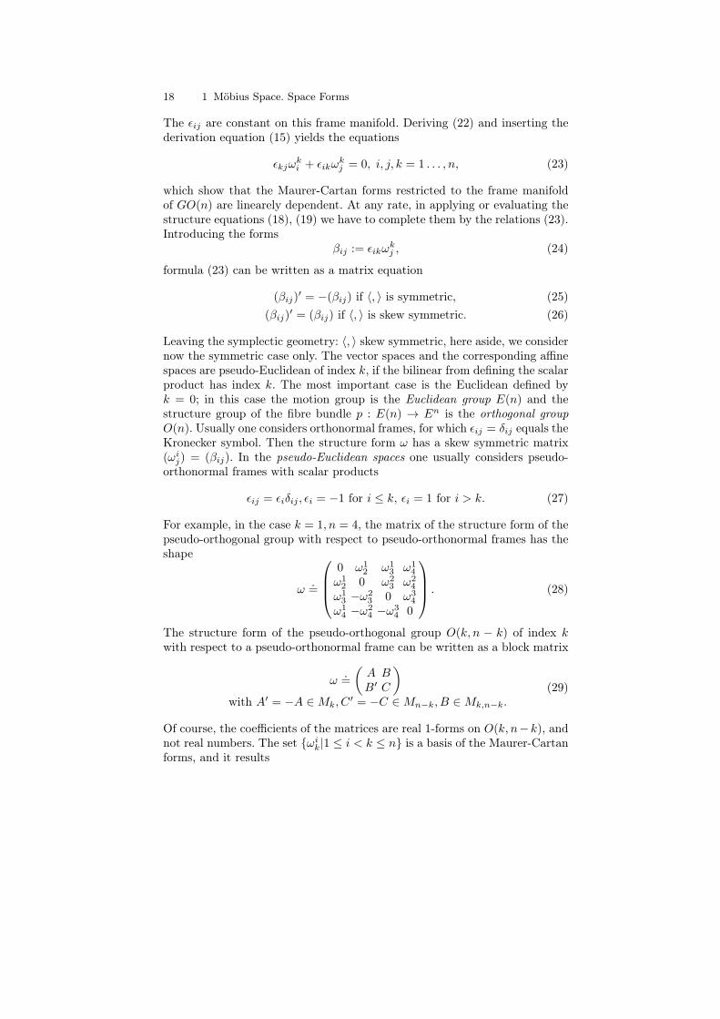
For example, in the case k = 1, n = 4, the matrix of the structure form of thepseudo-orthogonal group with respect to pseudo-orthonormal frames has theshape
ω.=
0 ω1
2 ω13 ω1
4
ω12 0 ω2
3 ω24
ω13 −ω2
3 0 ω34
ω14 −ω2
4 −ω34 0
. (28)
The structure form of the pseudo-orthogonal group O(k, n − k) of index kwith respect to a pseudo-orthonormal frame can be written as a block matrix
ω.=
(A BB′ C
)with A′ = −A ∈ Mk, C
′ = −C ∈ Mn−k, B ∈ Mk,n−k.(29)
Of course, the coefficients of the matrices are real 1-forms on O(k, n−k), andnot real numbers. The set ωi
k|1 ≤ i < k ≤ n is a basis of the Maurer-Cartanforms, and it results

1.3 Structure Forms 19
dimO(k, n− k) = n(n− 1)/2 (30)
for all k, 0 ≤ k ≤ n. For the pseudo-Euclidean point space Enk , that is the
affine space An under the action of the pseudo-Euclidean group E(n, k) beinggenerated by O(k, n − k) ⊂ GL(Wn) and the translations, we must enlargethe structure form according to (11), where now C ∈ O(k, n− k) is valid. Asin the affine geometry in the foregoing example we get a frame bundle as aprincipal fibre bundle
p : E(n, k) → Enk = E(n, k)/O(k, n− k) (31)
analogously to (13), the connected components of the fibres, the cosets
p−1(x) = gO(k, n− k), c0 = ga0 = a0 + x,
are the solutions of the completely integrable Pfaffian system
ω1 = ω2 = . . . = ωn = 0. (32)
2
1.3.2 The Structure Form of the Möbius Group
As pointed out in section 1, the Möbius group M(n) consists of two connectedcomponents of the pseudo-orthogonal group O(1, n + 1), see Propostion 1.1and (1.7). For certain purposes, e.g. investigating the geometry of circles orsubspheres, it may be convenient to work with pseudo-orthonormal frames.Then the formulas of example 2 in the special case k=1 may be applied,in particular formula (29) for the structure form. For the geometry of theMöbius space Sn itself, as a manifold of points, it is useful to work withisotropic-orthonormal frames defined by (1.9), see also Proposition 1.3 andformula (1.11). Thus we consider the group space M(n) as the manifold afall time-oriented isotropic -orthonormal frames; formulas (1.9) and (2.12) arevalid. The Gram matrix of any isotropic-orthonormal frame is
(ϵij) =
0 o′ −1o In o−1 o′ 0
, i, j = 0, . . . , n+ 1. (33)
Here In denotes the unit matrix of order n. Evaluating the relations (23),where the indices now run from 0 to n+ 1, one obtains
ωn+10 = ω0
n+1 = 0, ω00 = −ωn+1
n+1 , (34)
ωi0 = ωn+1
i , ω0i = ωi
n+1, (35)
ωij + ωj
i = 0 for i, j = 1, . . . , n. (36)
Thus the matrix of the structure form has the block structure
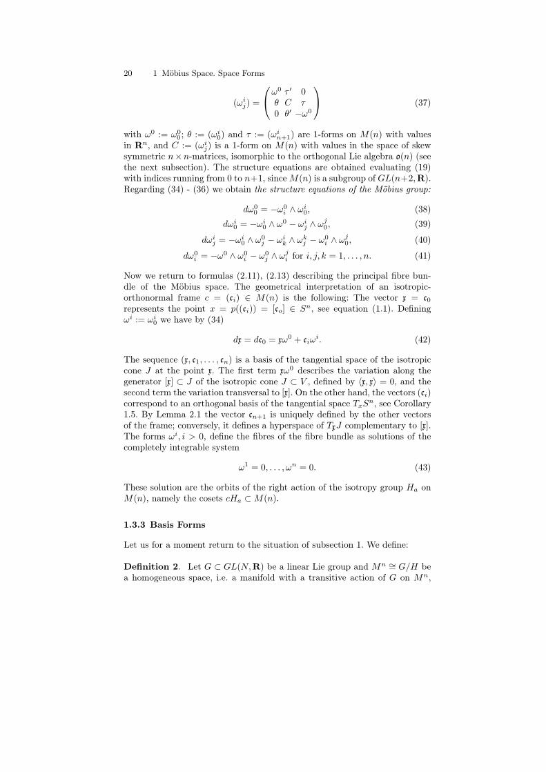
20 1 Möbius Space. Space Forms
(ωij) =
ω0 τ ′ 0θ C τ0 θ′ −ω0
(37)
with ω0 := ω00 ; θ := (ωi
0) and τ := (ωin+1) are 1-forms on M(n) with values
in Rn, and C := (ωij) is a 1-form on M(n) with values in the space of skew
symmetric n×n-matrices, isomorphic to the orthogonal Lie algebra o(n) (seethe next subsection). The structure equations are obtained evaluating (19)with indices running from 0 to n+1, since M(n) is a subgroup of GL(n+2,R).Regarding (34) - (36) we obtain the structure equations of the Möbius group:
dω00 = −ω0
i ∧ ωi0, (38)
dωi0 = −ωi
0 ∧ ω0 − ωij ∧ ωj
0, (39)
dωij = −ωi
0 ∧ ω0j − ωi
k ∧ ωkj − ω0
i ∧ ωj0, (40)
dω0i = −ω0 ∧ ω0
i − ω0j ∧ ωj
i for i, j, k = 1, . . . , n. (41)
Now we return to formulas (2.11), (2.13) describing the principal fibre bun-dle of the Möbius space. The geometrical interpretation of an isotropic-orthonormal frame c = (ci) ∈ M(n) is the following: The vector x = c0represents the point x = p((ci)) = [co] ∈ Sn, see equation (1.1). Definingωi := ωi
0 we have by (34)
dx = dc0 = xω0 + ciωi. (42)
The sequence (x, c1, . . . , cn) is a basis of the tangential space of the isotropiccone J at the point x. The first term xω0 describes the variation along thegenerator [x] ⊂ J of the isotropic cone J ⊂ V , defined by ⟨x, x⟩ = 0, and thesecond term the variation transversal to [x]. On the other hand, the vectors (ci)correspond to an orthogonal basis of the tangential space TxS
n, see Corollary1.5. By Lemma 2.1 the vector cn+1 is uniquely defined by the other vectorsof the frame; conversely, it defines a hyperspace of TxJ complementary to [x].The forms ωi, i > 0, define the fibres of the fibre bundle as solutions of thecompletely integrable system
ω1 = 0, . . . , ωn = 0. (43)
These solution are the orbits of the right action of the isotropy group Ha onM(n), namely the cosets cHa ⊂ M(n).
1.3.3 Basis Forms
Let us for a moment return to the situation of subsection 1. We define:
Definition 2. Let G ⊂ GL(N,R) be a linear Lie group and Mn ∼= G/H bea homogeneous space, i.e. a manifold with a transitive action of G on Mn,

1.3 Structure Forms 21
where H denotes the isotropy group of the arbitrarily fixed point a ∈ Mn. Abasis (ωi), i = 1, . . . , N := dimG of the Maurer-Cartan forms of G is nameda basis adapted to the homogeneous space, if the cosets gH ⊂ G are solutionsof the completely integrable Pfaffian system (43). The forms ωi, i = 1, . . . , n,are called basis forms of the homogeneous space Mn ∼= G/H. 2
Formula (43) contains the basis forms of the Möbius space. Example 1shows that the basis considered there is adapted to the affine space; the forms(ωi) are basis forms, and the same considerations show that they are basisforms for the Euclidean and pseudo-Euclidean spaces too. We prove
Lemma 4. Let p : g ∈ G 7→ gH ∈ Mn := G/H be the principal fibre bundleassociated to the homogeneous space Mn. Then there exist adapted bases ofthe Maurer-Cartan forms of G.
P r o o f. In the theory of Lie groups is proved the basic fact that the isotropygroups of a Lie transformation group [G,Mn] are closed Lie subgroups of G.Thus the fiber bundle p : G → G/H is analytic. Consider the unit elemente ∈ H ⊂ G. If dimG = r we have dimH = r − n. For the tangential spacesat e we have TeH ⊂ TeG, and there exist a basis (ωi
e), i = 1, . . . , n, of theannihilator TeH
⊥ ⊂ T ∗e G of TeH. Then the Pfaffian forms on G defined by
ωi(g, t) := ωie(dL
−1g (t)), i = 1, . . . , n, (t ∈ TgG), (44)
are left invariant. We complete them to a basis (ωρ), ρ = 1, . . . r, of theMaurer-Cartan forms of G. For the tangential space of the cosets we have
TggH = (dLg)eTeH,
and from (44) one obtains ωi(t) = 0 for all t ∈ TgH, showing that the cosetsare solutions of the Pfaffian system (43). 2
To find invariant geometric properties of the homogeneous space Mn byE. Cartan’s method of moving frames one has to consider local sections ofthe associated principal fibre bundle. Generally, if p : F r → Mn is a smoothsurjective map of differentiable manifolds and U ⊂ Mn an open subset, asmooth map s : U → F r is said to be a local section of p, if p s = idU . Incase that p is the projection of a fibre bundle one also names s a local sectionof the fibre bundle. The condition for s to be a local section implies
rank dsx = rank dpg = dimMn = n (45)
and it follows
Lemma 5. Let G be a linear Lie group. For any local section s : U → Gof the principal fibre bundle p : G → Mn = G/H the local structure forms∗ω = ω ds = (s∗ωi
j) is a matrix of 1-forms defined on U. If (ωi), i =1, . . . , r = dimG, is a basis of the Maurer-Cartan forms adapted to G/H, theforms σi(x) := ωi dsx, i = 1, . . . , n, are a basis of the dual tangential spaceT ∗xM
n. 2

22 1 Möbius Space. Space Forms
1.3.4 Lie Algebras
For a deeper understanding of the structural background of E. Cartan’smethod of moving frames the knowledge of some elementary facts about thestructure of Lie groups and Lie algebras is useful. 2 The Lie algebra g of theLie group G is the set of all left invariant vector fields on the Lie group G.Let e ∈ G denote the unit element. Then for any tangential vector Xe ∈ TeGthere exists a uniquely defined left invariant vector field, namely
X(g) := (dLg)eXe with X(e) = Xe.
Argumentwise addition and multiplication with scalars λ ∈ R give g thestructure of an r-dimensional real vector space, r = dimG, which is the dualof the space of the Maurer-Cartan forms. Clearly θ(X) = constant for anyMaurer-Cartan form θ and any X ∈ g. Since the map X ∈ g 7→ X(e) ∈ TeGis a linear isomorphism one often identifies g with TeG.
Considering the vector fields as differential operators, the commutator oftwo vector fields is defined by
[X,Y ](f) := X(Y (f))− Y (X(f)), f ∈ C∞(G); (46)
it is a vector field again, and it is left invariant if X,Y have this property. Thecommutator is a bilinear operation [, ] : g× g → g being anti-commutative
[X,Y ] + [Y,X] = 0 (47)
and satisfying the Jacobi identity:
[[X,Y ], Z] + [[Y, Z], X] + [[Z,X], Y ] = 0. (48)
Generally, a vector space g over a commutative field K, on which a commu-tator operation [, ] is defined, is called a Lie algebra. A trivial example oneobtains setting [X,Y ] := 0 for all X,Y ∈ g; such a Lie algebra is named anAbelian Lie algebra. Another interesting example is the infinite dimensionalLie algebra of all vector fields of class C∞ on a differentiable manifold Mn withthe commutator defined by (46). Later on we will describe the Lie algebras ofthe pseudo-orthogonal groups, in particular, the Möbius group..
The following fundamental theorem summarizes the main relations be-tween Lie groups and Lie algebras (see C. Chevalley [6], S. Helgason [9]):
Theorem 6. The map G 7→ g, ϕ ∈ Hom(G,H) 7→ dϕ ∈ Hom(g, h) is acovariant functor of the category of Lie groups with the continuous homo-morphisms as morphisms into the category of the finite dimensional real Lie
2 The matter necessary for our purposes is contained in [30]. For a profound treat-maent see S. Helgason [9], where numerous hints to the literatur about Lie theorycan be found.

1.3 Structure Forms 23
algebras. This functor maps Lie subgroups to Lie subalgebras of the same di-mension, and normal Lie subgroups to ideals of the corresponding Lie algebras.Lie groups with isomorphic Lie algebras are locally isomorphic. To any finitedimensional real Lie algebra there exists up to isomorphism exactly one con-nected, simply connected Lie group whose Lie algebra is isomorphic to thegiven one. 2
We remark that a continuous homomorphism of Lie groups is always ana-lytic, thus its differential is defined; it maps left invariant fields to left invariantfields. To characterize dϕ it suffices to know the differential at the unity dϕe.
Now we can define the structure form ω of the Lie group G as the one-Formon G with values in the Lie algebra g of G generalizing (3):
ω : t ∈ TgG 7−→ ω(t) := dL−1g t ∈ TeG = g,
or shortly ω = g−1dg. Again ω is left invariant. The rule (6) generalizes to
R∗aω = Ad(a−1) ω,
where Ad(a) := dLa dRa−1 denotes the adjoint representation of the Liegroup (see also (51) below).
Let(Xi), i = 1, . . . , r = dim g, be a basis of the Lie algebra g. Decomposingthe commutator
[Xi, Xj ] = XkCkij , i, j, k = 1, . . . , r,
we obtain the structure constants of the Lie algebra g, being the coordinatesof a twofold covariant, onefold contravariant tensor defining the Lie algebrastructure and, by Theorem 6, locally also the Lie group. Let (ωi) be the dualbasis for the Maurer-Cartan forms:
ωi(Xj) = δij .
For any Maurer-Cartan form θ and any left invariant vector field X ∈ g thevalue θ(X) is constant. Thus the general formula for the value of the exteriordifferential of a Pfaffian form on arbitrary vector fields X,Y (see [30], (II.4.51))
dθ(X,Y ) = Xθ(Y )− Y θ(X)− θ([X,Y ])
yieldsdωi(Xj , Xk) = −ωi(XhC
hjk) = −Ci
jk.
On the other hand, decomposing the exterior differentials dωi with respect tothe natural basis (ωj ∧ ωk), j < k, in the space of biforms, one obtains withthe same constants
dωi = −1
2Ci
jkωj ∧ ωk = −
∑j<k
Cijkω
j ∧ ωk.
24 1 Möbius Space. Space Forms
Comparing this with the structure equations (9) of the general linear groupGL(n,R) we recognize the deep meaning of these equations: they define thestructure of the linear Lie groups. In the case that G ⊂ GL(n,R) is not thefull linear group, the forms ωi
j restricted to G are Maurer-Cartan forms on G.In case dimG < n2 they are linearely dependent. Since exterior differentiationcommutes with restriction of the forms, the structure equations (9) are validfor the forms restricted to G. Regarding the linear depedicies as we will do inthe examples considered later one one obtaines the structure equations for Gevaluating (9).
The main tool for relating the properties of a Lie group with those of thecorresponding Lie algebra is the exponential, which we are going to definenow. Let g be the Lie algebra of the Lie group G and X ∈ g a left invariantvector field. Then the solution of the differential equation
dg
dt= X(g) with g(0) = e
is uniquely defined and exists for all t ∈ R; we denote it by exp tX. By the leftinvariance of X the trajectory of the field X(g) through the element g ∈ G isgiven by g(t) = g exp tX, and it follows
exp(s+ t)X = exp sX exp tX.
Corollary 7. For any X ∈ g the map t ∈ R 7→ exp tX ∈ G is an analytichomomorphism of the additive group [R,+] into the Lie group G, named aone-parameter subgroup. Every connected one-dimensional Lie subgroup ofthe Lie group G is such a one-parameter subgroup; thus it is Abelian.2
The Lie subalgebra corresponding to the one-parameter subgroup exp tXis the vector subspace of g spanned by X; it is an Abelian subalgebra. Nowwe define the exponential exp of the Lie group G as the map
exp : X ∈ g 7−→ expX := exp tX|t=1 ∈ G. (49)
We prove
Lemma 8. The map exp : g → G is analytic. There exists a neighbourhoodU of the zero element 0 ∈ g such that exp |U is an analytic diffeomorphism ofU onto the neighbourhood exp(U) ⊂ G of the unity e ∈ G.
P r o o f. The solution of the differential equation depends analytically on theparameter X. For the differential of exp at the zero element 0 one obtains
(d exp)0(X) =d exp tX
dt|t=0 = X,
and it follows d exp0 = idg. By the inverse function theorem the map exp isinvertible in a certain neighbourhood U of 0.2

1.3 Structure Forms 25
For any a ∈ G the inner automorphism σa is defined by
σa(g) := a · g · a−1, g ∈ G. (50)
Obviously, one has σa = La Ra−1 . By Theorem 6 the differential dσa is anautomorphism of the Lie algebra g. One easily proves
Corollary 9. For any Lie group G with Lie algebra g the map
Ad : a ∈ G 7−→ Ad(a) := dσa ∈ Aut(g) (51)
is a representation of G as a group of automorphisms of the Lie algebra g,called the adjoint representation of G. 2
Clearly the relationAd(a · b) = Ad(a) Ad(b)
is fulfilled for all a, b ∈ G.
Example 3. Now we specialize to the case of linear Lie groups and Lie al-gebras, see e. g. H. Freudenthal, H. De Vries [8]. The general linear groupconsists of all real non-degenerate matrices
g ∈ GL(n,R) ⇐⇒ g = (γij) ∈ Mn(R) with det(γi
j) = 0;
thus it is an open set in the real vector space Mn(R) of real square matricesof order n with coordinates γi
j ; its dimension is n2. The group operation isthe usual matrix product. The corresponding Lie algebra is the vector space
gl(n,R) = TeGL(n,R) ∼= Mn(R),
with the matrix commutator
[X,Y ] := X · Y − Y ·X. (52)
For any X ∈ gl(n,R) the infinite series of matrices
etX :=∞∑k=0
(tX)k
k!(53)
converges for all values of t. The well known formula
det(eX) = etrX , (54)
where trX denotes the trace of the matrix X, implies det(eX) = 0, andderiving (53) one gets
d(etX)
dt= etX ·X = X · etX . (55)

26 1 Möbius Space. Space Forms
Therefore etX is the trajectory of the left invariant vector field X(g) = g ·Xthrough the unity e0X = e = (δij) and coincides with the exponential definedfor general Lie groups. The differentials dγi
j form a cobasis at the point e =
(δij); one has
dγij(X) = ξij for X = (ξkl ) ∈ Mn(R) = TeGL(n,R),
thus the corresponding basis of TeGL(n,R) consists of all matrices
Xkl = (δilδ
kj )i,j ,
which have the coordinates ξkl = 1 and ξij = 0 if i = k or j = l. The lefttranslation of these vectors resp. forms give the basis of the Lie algebra resp.the Maurer-Cartan forms as fields on GL(n,R). Since the group multiplicationis generated by the bilinear matrix multiplication, the adjoint representationof GL(n,R) can be expressed as a product of matrices
Ad(a)(X) = a ·X · a−1 with a ∈ GL(n,R), X ∈ gl(n,R). (56)
The next example treats the Lie algebras of some important classes of linearLie groups G ⊂ GL(n,R). 2
Example 4. Now we consider the n-dimensional real vector space Wn witha distinguished scalar product, as in Example 2. By (21) the linear groupGO(n) is defined as the group of all linear transformations preserving thescalar product. Obviously, formulas (52) - (56) are valid for any linear groupas a subgroup of GL(n,R). Let X belong to the Lie algebra go(n) = TeGO(n).Then the corresponding one-parameter subgroup belongs to GO(n), and by(21) we have
⟨etX x, etX y⟩ = ⟨x, y⟩ for all x, y ∈ Wn.
Deriving this equation we obtain applying (55)
d⟨etX x, etX y⟩dt
= ⟨X etX x, etX y⟩+ ⟨etX x, X etX y⟩ = 0. (57)
Setting t = 0 we get a linear equation for X:
⟨Xx, y⟩+ ⟨x, Xy⟩ = 0 for all x, y ∈ Wn. (58)
Conversely, if an element X ∈ gl(n,R) satisfies (58), one may apply it for thevectors etX x, etX y, and it follows (57). The scalar product is constant, andthe one-parameter subgroup belongs to GO(n). Equation (58) characterizesthe Lie algebra go(n) of GO(n). Considering the matrix (ξij) of X with respectto a basis (ai) of Wn:
Xaj = akξkj ,
we obtain a system of homogeneous linear equations defining the Lie subalge-bra go(n) ⊂ gl(n,R):

1.3 Structure Forms 27
ϵkjξki + ϵikξ
kj = 0, (59)
where (ϵkl) = gr denotes the Gram matrix (20). The system (59) formallycoincides with (23) for the Maurer-Cartan forms of GO(n). This has to be ex-pected: by definition (3) the structure form is a 1-form on GO(n) with valuesin the Lie algebra go(n). If Wn is the Euclidean vector space and (ai) an or-thonormal basis, gr is the unit matrix; formula (59) shows that the orthogonalLie algebra o(n) is represented as the space of all skew symmetric matricesof order n, the forms (ωi
j)i<j , are a basis of the Maurer-Cartan forms of theorthogonal group O(n). The structure equations (9) remain valid; on O(n) onehas to take into account the skew symmetry ωi
j = −ωji implying ωi
i = 0 forall i = 0, . . . , n. Analogue considerations are valid for the pseudo-orthogonalgroups O(k, n − k); formula (29) can be interpreted as the characterizationof the Lie algebra o(k, n − k). Finally, formula (17) gives the matrix repre-sentation of the affine Lie algebra a(n), and, if the corresponding symmetryrelations (29) of the part (ωi
j) of the matrix are taken into account, also theLie- algebras of the Euclidean resp. pseudo-Euclidean groups. 2
1.3.5 Linear Isotropy Representations
Let the Lie group G act smoothly on the differentiable manifold Mn. Thenthe geometrical properties of the transformation group [G,Mn] depends es-sentially on the linear isotropy representations:
Definition 3. Let [G,M ] be a Lie transformation group and
Ha = g ∈ G|g(a) = a
the isotropy group of the point a ∈ M . Then the map
ϕa : h ∈ Ha 7−→ ϕa(h) := (dlh)a ∈ GL(TaM) (60)
is a linear representation of Ha, named the linear isotropy representation ofthe transformation group [G,M ] at a ∈ M . 2
Clearly, if b = ga lies on the same G-orbit, the isotropy groups are isomorphic:Hb = gHag
−1, and the same is true for the isotropy representations:
ϕb(h) = (dlg)a ϕa(g−1hg) (dlg)−1
a , h ∈ Hb, b = ga ∈ M.
Especially, all the linear isotropy representations ϕa at the points of a ho-mogeneous space M = G/H are equivalent, and one speaks about the linearisotropy representation of this space. One easily shows that the G-invarianttensor fields on a homogeneous space M are defined by the Ha-invariant ten-sors of the linear isotropy representation. We remember the following nota-tions: If t is a tensor on the vector space V and h : V → W a linear iso-morphism, the image h∗t is a well defined tensor on W . If h : Mn → Ln is

28 1 Möbius Space. Space Forms
a diffeomorphism and t : x ∈ Mn 7→ t(x) is a tensor field on Mn, then theimage h∗t is defined as the tensor field on Ln by
h∗t : y ∈ Ln 7−→ h∗t(y) := (dhx)∗t(x), where x = h−1(y). (61)
A tensor field t on the space Mn of a transformation group [G,Mn] is G-invariant, if g∗t = t is true for any transformation g ∈ G.
Lemma 10. Let Mn ∼= G/Ha be a homogeneous space. Then there existsa G-invariant tensor field t = t(x) over Mn if there is a tensor ta of thecorresponding type at the origin a ∈ Mn invariant under the linear isotropyrepresentation: (dha)∗ta = ta for all h ∈ Ha. If ta is such a Ha-invarianttensor at the point a, then
t : x = gHa ∈ Mn 7−→ t(x) := (dlg)a∗ta (62)
is the uniquely defined G-invariant tensor field on Mn with t(a) = ta. 2
Indeed, the invariance of ta with respect to the linear isotropy representationimplies that t(x) does not depend on the transformation g ∈ x = gHa mappinga into x.
The basis forms ωi play a central role in the differential geometry of ho-mogeneous spaces. Therefore we return for the moment to the general theoryconsidering the situation of the last subsection: Let
p : G −→ Mn = G/H, ω = g−1dg : TG −→ g,
be the principal fibre bundle corresponding to the homogeneous space G/Hof a Lie group G with Lie algebra g, H = Ha the isotropy group of the pointa ∈ Mn, ω the structure form on G. Let the Maurer-Cartan forms ωi be abasis of the annihilator h⊥ = [ω1, . . . , ωn] of the Lie subalgebra h ⊂ g of theisotropy group H. The form
θ := q ω : TG −→ g/h, (63)
where q : g → g/h denotes the canonical projection, is named the canonicalform of the homogeneous space G/H; the forms ωi, i = 1, . . . , n, are thecomponents of the canonical form θ. Since ωi(h) = 0, the definition
ωi(Xmod h) := ωi(X) for Xmod h ∈ g/h
yields a cobasis for the vector space g/h. The forms ωi, i = 1, . . . n, coincidewith the basis forms of the homogeneous space Mn = G/H defined in subsec-tion 3. Using (51) we see that the Lie subalgebra h remains invariant underthe action of the adjoint representation of G restricted to H: Ad(h)h = h forall h ∈ H; therefore formula
Ad(h)(Xmod h) := Ad(h)(X)mod h, h ∈ H,Xmod h ∈ g/h, (64)

1.3 Structure Forms 29
defines the adjoint representation Ad of H on g/h. This definition implies
Ad(h) q = q Ad(h), h ∈ H, (65)
and equation (6) yields immediately: The canonical form θ is a left invariant1-form of type Ad on G with values in g/h. The latter means
R−1∗h (θ) = Ad(h) θ for all h ∈ H. (66)
The geometrical meaning of the adjoint representation Ad lies in the fact thatit may serve as an algebraic model of the linear isotropy representation:
Lemma 11. The linear isotropy representation of a homogeneous space G/His equivalent to the adjoint representation Ad of the isotropy group H on thefactor space g/h.
P r o o f. We identify g = TeG. The differential dpe of the projection p :G → G/H at the point e has the kernel h = TeH, being the tangential space ofthe fibre eH = H at e. Thus we have an uniquely defined linear isomorphismp : g/h → TaM , M = G/H, satisfying
p(XmodH) = dpe(X), X ∈ g.
From this relation and (64) it follows for h ∈ H:
p(Ad(h)(Xmod h)) = p(Ad(h)(X)mod h) = dpe(Ad(h)(X)).
Now we use the definition (51) of the adjoint representation
Ad(g) = dLg (dR−1g )e
and the obvious relations
p Rh = p for h ∈ H, p Lg = lg p for g ∈ G, (67)
and obtain at the origin a = p(e):
dpe(Ad(h)(X)) = dpe dLh dRh−1(X) = dlh(dpe(X)) = dlh(p(Xmod h)),
what proves the lemma. 2
1.3.6 Applications to Möbius Geometry
Again we return to Möbius geometry, G = M(n),Mn = Sn. At the end ofsubsection 2 we pointed out that the Maurer-Cartan forms ωi := ωi
0, i =1, . . . , n, span the annihilator of the isotropy algebra ha; thus they are basisforms and the components of the canonical form θ of the Möbius space. The

30 1 Möbius Space. Space Forms
matrix of the elements h ∈ Ha of the isotropy group are given by (1.11); oneeasily calculates
h(A, a, λ)−1 = h(A−1,−A−1aλ−1, λ−1). (68)
For the structure form of the linear group one proves using matrix multipli-cation: Is (ωi
j) ∈ gl(N,R) the matrix of an element of the linear Lie algebraand (γi
k) ∈ GL(n,R) a group element g, then the matrix of Ad(g)(ω) is
Ad(g)(ω).= (ωi
j) := (γik)(ω
kl )(γ
lj)
−1. (69)
Applying this and (68) for g = h(A, a, λ) one obtains for the base forms thetransformation rule
ωi = γikω
kλ with A = (γik) ∈ O(n). (70)
Since the representation Ad is equivalent to the linear isotropy representation,it follows from Lemma 11:
Proposition 12. The transformation rule of the basis forms of the Möbiusspace is given by (70). Therefore the symmetric bilinear form
φ(s, t) :=n∑
i=1
ωi(s)ωi(t), s, t ∈ g/h, (71)
transforms under the action of h = h(A, a, λ) ∈ Ha obeying the rule
φ(Ad(h)(s), Ad(h)(t)) = φ(s, t)λ2 (72)
The linear isotropy representation of the Möbius space has the kernel
K := h(In, a, 1) ∈ Ha|a ∈ Rn (73)
being isomorphic to the abelian group [Rn,+].
P r o o f. The transformation rule (72) immediately follows from (70) since Ais an orthogonal matrix. Also by (70) it results that the dual basis (ωi) ofg/h remains fixed iff A is the unit matrix and λ equals 1. The last statementfollows from (1.11) by a direct calculation. 2
From Proposition 12 and Lemma 10 the existence of a positive definitescalar product invariantly defined up to a positive factor on the Möbius spacecan be concluded: Obviously, such a scalar product φa exists on the tangentialspace TaS
n at the origin a = p(e), invariantly up to a positive factor underthe action of the linear isotropy representation. Then the definition
φx(s, t) := φa(dl−1g (s), dl−1
g (t)) if x = ga, s, t ∈ TxSn,

1.3 Structure Forms 31
extends φa to a scalar product with the mentioned properties over Sn, thusdefining a class of conformally equivalent Riemannian metrics on the n-sphere.This definition is a special case of (61).
We shall give another proof of this fact using the method of moving frames.This method has the advantage that the scalar product is given by an expres-sion appropriate for explicit calculations, and basic for the Möbius differentialgeometry. Let U ⊂ Sn be an open subset, and let s(x) = (ci(x)) ∈ M(n),s(x) = (ci(x)), x ∈ U be two moving frames defined on U . Then h = s−1s ∈Ha is an element of the isotropy group depending on x ∈ U , and we have thetransformation rule of the moving frames
s(x) = s(x).h−1(x), x ∈ U, h(x) ∈ Ha. (74)
We consider the local basis forms σi = s∗ωi, σi = s∗ωi, satisfying
dc0 = ciσi
and the corresponding equation for the differential dc0 on U . From (1.11) and(68) we get
c0 = c0λ, ci = c0γ0i + cjγ
ji with (γj
i ) ∈ O(n).
Deriving the first equation we obtain from
dc0 = dc0λ+ c0dλ
for the transformed coefficients
σi = ⟨dc0, ci⟩ = σjγijλ with (γj
i ) ∈ O(n). (75)
It follows
Proposition 13. For any local isotropic-orthonormal moving frame on anopen set U ⊂ Sn with the basis forms σi = ⟨dc0, ci⟩ the bilinear form
φ(s, t) := ⟨dc0, dc0⟩ =n∑
i=1
σi(s)σi(t), s, t ∈ TxSn,
defines a positive definite scalar product on the tangential spaces TxSn up to
a factor λ2 > 0, depending on the choice of the frame s(x) ∈ p−1(x). Thusthe angle α of the tangential vectors is correctly defined in the usual way:
cosα :=φ(s, t)
|s||t|with |s| :=
√φ(s, s). (76)
2
32 1 Möbius Space. Space Forms
Usually one speaks about the conformal geometry of a Riemannian space asthe theory of the properties invariant under arbitrary renormings of the Rie-mannian metric. In particular, if one takes the local moving frames with theproperties c0 = x ∈ Sn
1 and ti = ci ∈ TxSn1 , the induced Riemannian metric
coincides with the standard Riemannian metric of constant curvature 1 onthe unit n-sphere. By (1.11) and (75) it is clear that any positive renormingfunction on Sn may be realized by an appropriate choice of the moving frameg = g(x). Therefore the conformal properties of the standard metric of thesphere Sn are also Möbius invariant properties. Clearly, not every renormingof the standard metric may be obtained by a Möbius transformation, depend-ing on a finite number of parameters. It must be expected that the Möbiusgeometry as the theory of properties invariant under the action of the Möbiusgroup is more special than the conformal geometry of the sphere.
By a theorem of A. Lichnérowicz, see § 30, p. 47 in [15], the linear isotropyrepresentation is true, i.e. its kernel K is trivial, if on the homogeneous spaceMn = G/H with an effective action of G there exists a G-invariant linearconnection. Thus we conclude:
Corollary 14. On the Möbius space Sn = M(n)/Ha does not exist nei-ther a Möbius-invariant linear connection nor a Möbius-invariant pseudo-Riemannian structure. 2
Therefore the base invariant of Möbius geometry is the class of Rieman-nian metrics Möbius equivalent to the standard metric on Sn, induced by itsembedding as the unit sphere into the Euclidean space En+1.
1.3.7 Applications to the Space Forms Enc
In this subsection we calculate the structure forms and the canonical forms ofthe space forms En
c and relate them to the structure form of the Möbius group.To this aim we consider the bundles of orthonormal frames Oc(n) over En
c andtheir embeddings into the Möbius group described in Proposition 2.2, (2.22),and (2.23). The vector c0 = x of the moving frame is uniquely defined by theembedings (2.3), (2.4), and (2.5) of the space forms. The ci, i = 1, . . . , n, forman orthonormal basis of the tangential space TxE
nc , and the complementary
vector cn+1 is defined by Proposition 2.2. The structure forms of the isometrygroups of the space forms considered as subgroups of the Möbius group M(n)are the restrictions of the structure form of M(n) onto these subgroups. Itfollows in each of the cases
ω0 = −⟨dx, cn+1⟩ = 0, (77)
and from (42) we conclude
dx =
n∑i=1
ciωi. (78)
1.3 Structure Forms 33
Since the isotropy group of the space forms is the orthogonal group O(n)embedded into M(n) by (24), we have λ = 1 in the transformation rules (70),(72), and (75). We conclude applying Proposition 12
Corollary 15. On all n-dimensional space forms Enc the isotropy groups are
isomorphic to the orthogonal group O(n). The linear isotropy representationsare the standard representation of O(n) on the Euclidean vector space En;thus they are true. The bilinear form φ defined by (71), restricted to the bun-dle of orthonormal frames of the space forms En
c , defines an Oc(n)-invariantRiemannian metric on these spaces. 2
Now, differentiating the vectors cn+1 defined by (23), we calculate the formsin the block τ of the restricted structure form (37) of M(n):
ω0i = ωi
n+1 = ⟨ci, dcn+1⟩ = −cωi/2, (79)
where c = r−2, c = −r−2, and c = 0 are the constant curvatures of thespherical, hyperbolical resp. Euclidean spaces En
c . Inserting (77) and (79)into the structure equations (38) - (41) of the Möbius group, one proves
Proposition 16. The structure form of M(n) restricted to the isometry groupOc(n), c = r−2, c = −r−2, or c = 0, has the block matrix 0 −(ωic/2)′ 0
(ωi) (ωij) −(ωic/2)
0 (ωi)′ 0
, with ωij + ωj
i = 0, i, j = 1, . . . , n. (80)
The canonical form is given by (78) with θ = dx. The structure equations ofthe spaces of constant curvature En
c may be written in the following shape:
dωi + ωij ∧ ωj = 0, (81)
dωij + ωi
k ∧ ωkj = cωi ∧ ωj . (82)
P r o o f. Formula (80) follows from (77) and (79). Inserting these equationsinto the structure equations of the Möbius group (38)-(41) one sees: (38)reduces to the trivial equation 0 = 0, (81) and (82) result from (39) and (40),and (41) is equivalent to (81) if c = 0, and trivial else. Since the structureform of Oc(n) is the restriction of that of M(n) and exterior differentiationcommutes with restrictions, Proposition 16 is proved. 2
In difference to the Möbius geometry the differential geometry of the spacesof constant curvature is a special Riemannian geometry, and the structureequations (81), (82) are special cases of E. Cartan’s structure equations of aRiemannian manifold, or more generally, a manifold with a linear connection.In particular, the left side of (82) are the components Ωi
j of the curvatureform of the linear connection, see e.g. S. Kobayashi, K. Nomizu [14], or R. Su-lanke,P. Wintgen [30], Satz II.10.4, p.160:
34 1 Möbius Space. Space Forms
Ωij := dωi
j + ωik ∧ ωk
j =1
2Ri
jklωi ∧ ωj , Ri
jkl +Rijlk = 0. (83)
The functions Rijkl are the coordinates of a tensor, the curvature tensor of
the space. In case of the spaces of constant curvature from (82) it followsRi
jkl = δijδklc, the coordinates of the curvature tensor are zero or the sameconstant c, or, what is the same, the sectional curvature of these Riemannianspaces is constant. For details see the cited literature. E. Cartan’s exposition ofthe Riemannian geometry is contained in the book [5], edited by S. P. Finikovin Russian language. The monography [38] of J. A. Wolf contains a detailedstudy of the spaces of constant curvature and their generalizations.
2
The Möbius Structure of an Immersion
2.1 E. Cartan’s Method of Moving Frames
In the following we want to apply E. Cartan’s method of moving frames [4]to the Möbius geometry of immersions f : Y m → Sn, m = 1, . . . , n − 1,into the sphere Sn. In general, two immersions fi : Y m
i → Mn := G/H,i = 1, 2, are G-equivalent, if there exist a diffeomorphismus φ : Y1 → Y2 anda transformation g ∈ G such that f2 = g f1 φ−1. Often one identifies themanifolds Y1 = Y2 =: Y with the help of φ and assumes φ = idY ; in thiscase one speaks about the G-congruence of the immersions fi : Y
m → Mn,i = 1, 2. Clearly, these definitions yield equivalence relations in the classes ofimmersions under consideration. The first task is to characterize the equiva-lence classes by G-invariant geometric objects, like functions, tensor fields, orconnections, defined on the manifolds Y m. We do not want, and do not needhere, to explain the theory of geometric objects in full generality; a very niceand contemporary presentation of this theory, appropriate for our purposes,is contained in the article [22] of S. E. Salvioli. Let us illustrate the definingproperty of a geometric object, more precisely, a geometric object field, withthe example of a tensor field. A tensor field on the manifold Y m is a sectionof a tensor bundle over Y m:
y ∈ Y m 7−→ t(y) ∈ Tr,s(Y m) with p(t(y)) = y, (y ∈ Y m).
Here p : Tr,s(Y m) → Y m denotes the projection in the bundle of r-timescontravariant, s-times covariant tensors over Y m. Examples of tensor fieldsare functions (r = s = 0), vector fields (r = 1, s = 0), Pfaffian forms (r =0, s = 1), Riemannian metrics (r = 0, s = 2), curvature tensors, etc. Let Fm
denote a class of immersions of m-dimensional manifolds f : Y m → Mn intothe homogeneous space Mn closed under diffeomorphisms and the action of G,f 7→ g f, (g ∈ G). A map f ∈ Fm 7→ tf ∈ Γ (Tr,s(Y m)), where Γ (Tr,s(Y m))denotes the space of sections of the tensor bundle, is a G-invariant, if it isinvariant under the action of G:
36 2 The Möbius Structure of an Immersion
tgf = tf for all f ∈ Fm, g ∈ G.
and equivariant under the action of diffeomorphisms φ : Y m → Y m:
tf (y) = dφ∗(tf (φ−1(y))), (f = f φ−1, y ∈ Y m).
Here dφ∗ denotes the morphism of tensor bundles generated by the differ-ential of φ. All manifolds and maps are supposed to be sufficiently oftendifferentiable. The concepts of differentiable manifolds, tensor bundles, trans-formation groups etc. can be found in [30], in S. Kobayashi, K. Nomizu [14],[13], or other textbooks of differential geometry.
The main ideas of E. Cartan‘s method of moving frames [4] can be de-scribed as follows. Consider an immersion f : Y m → Mn = G/H of anm-dimensional smooth manifold into the n-dimensional homogeneous spaceMn, 0 < m < n. Realize the group space G as a space of moving frames, asbeing done in chapter 1 for the Möbius group and the isometry groups of thespace forms En
c . Let p : G → G/H be the canonical projection. Construct theinduced frame bundle with the bundle space as the disjoint union
F0(f) :=∪
y∈Y m
p−1(f(y))). (1)
In a canonical way, F0 = F0(f) is provided with the structure of a principalfibre bundle F0(Y
m, p,H) over Y m with structure group H and a bundlemorphism f such that the following diagram is commutative:
F0 G
Y m Mn
-f
?
p
?
p
-f
(2)
If f is injective, then also f is injective, and Fo can be identified with thesubset g ∈ G|p(g) ∈ f(Y m). If the group space G is interpreted as a bundleof frames, then the fibre p−1(y)) ⊂ F0 at the point y ∈ Y m consists of all theframes at the point f(y). The action of the isotropy group H on the fibres ispreserved by this construction; f as a bundle morphism fulfils (2) and
Rh f = f Rh, h ∈ H. (3)
Furthermore, the structure form ω on G induces by
ω0 := f∗ω := ω df (4)
a 1-form on F0 of typ Ad |H with values in the Lie algebra g of G, named thestructure form of order 0 of the immersion f . In the paper [25] the structure

2.1 E. Cartan’s Method of Moving Frames 37
just described is precised and subsumed under the concept of a G,H-structure[F0(Y
m, p,H), ω0].Clearly, G-equivalent immersions and, a fortiori, G-congruent immersions
induce isomorphic G,H-structures. On the other hand, in [29] we proved thatto each G,H-structure on a connected manifold Y m there exists an immer-sion of a certain covering manifold Y m of Y m, f : Y m → G/H, whose in-duced G,H-structure is locally isomorphic to the given one; this immersionis uniquely defined up to G-congruence. Therefore, locally or for simply con-nected Y m, the G-equivalence classes of immersions correspond bijectively tothe isomorphy classes of G,H-structures, and the classification can be donestudying the latter. E. Cartan’s method of moving frames consists of a stepby step adaption of the frames to the immersion, leading finally, in the mostconvenient case, to a uniquely defined canonical frame
s : y ∈ Y m 7−→ s(y) ∈ G with p(s(y)) = y. (5)
The canonical frames must be defined in a G-equivariant way, meaning thatG-congruent immersions possess G-congruent canonical frames. Then the co-efficients of the induced form s ∗ ω0 : TY m → g may serve as a completesystem of invariants for the classification of the immersions under consider-ation. Unfortunately, in general there exist canonical frames only for specialsubclasses of immersions into G/H, and one has to find such subclasses. Oftenthe adaption of frames may be carried out by successive natural reductionsFi+1 ⊂ Fi ⊂ F0 of the G,H-structure F0, leading to smaller structure groupsH0 = H ⊃ H1 . . . ⊃ Hk = e, in case of a canonical frame. This reduc-tion procedure has been carried out by E. Cartan in many special cases. Thegeneral theory and therewith the justification of the method has been givenindependentla by G. R. Jensen [11] and R. Sulanke, A. Švec [29], see also [25]for a global result. Another method to find G-invariants of the immersion isthe following: Consider local sections of the induced frame bundle Fi definedon open subsets U ⊂ Y m
s : y ∈ U 7−→ s(y) ∈ Fi with p(s(y)) = y, (6)
and study the induced form s∗ω : TY m|U → g. The components of s∗ω are 1-forms on U , and their transformation rules under a change of the local framescan be calculated using the adjoint representation of the group G restrictedto the structure group Hi: If s(y) = s(y)h−1(y) is the transformation of thelocal frames, we get
s∗ω = ω(dsy)= ω(dsy) dRh−1(y) + ω(s(y))(dh−1)y= Ad(h)(s∗ω − h−1dhy),
(7)
see formulas (3.9), (3.12) in [29]. Now, one often may construct G-invariantgeometric objects using this transformation rule, and express them in terms of

38 2 The Möbius Structure of an Immersion
the components of the structure form. Then, if sufficiently many invariants arefound, one conversely may construct the G,H-structure from these invariants;applying the immersion theorem in [29] one gets an existence and uniquenesstheorem for the class of immersions under consideration.
The main task in solving the classification problems is the step-by-stepreduction of the induced frame bundles. One has to describe the orbit structureof non-transitive transformation groups naturally related to the given class ofimmersions. Unfortunately, we don’t have a general method to handle thistask. Thus, the classification of immersions into a given homogeneous spaceis an interesting and, as a rule, not so simple task. E. Cartan’s method ofmoving frames not only gives a general framework to attack these problems,but also yields, by the general immersion theorem, an existence and uniquenesstheorem almost automatically. Its principal theoretical meaning consists of thefact that it bases the differential geometry of an homogeneous space Mn =G/H on the structure of the pair of Lie groups G ⊃ H defining the space.In the following I shall apply and illustrate this method in the differentialgeometry of the Möbius space. I have chosen just this space since 1. theredoes not exist an invariant metric nor an invariant linear connection – thusthe classical methods of differential geometry, like absolute differentiation, arenot applicable – and 2. the Möbius geometry is nearly related to the classicalgeometries of constant curvature, as pointed out in chapter 1, what gives thepossibility to interpret the Möbius invariants in metric, in particular Euclideanterms, in this way investigating their geometrical meaning.
2.2 The Möbius Structure of an Immersion
In this section we consider immersions f : Y m → Sn = M(n)/Ha, 0 < m < n,into the Möbius space. We use the denotations defined in chapter 1; M(n) isthe Möbius group, whose group space is identified with the manifold of allisotropic-orthonormal frames; Ha ⊂ M(n) is the isotropy group of the origin,the point a = [a0], and (ai) a fixed isotropic-orthonormal basis of the pseudo-Euclidean vector space V n+2 of index 1, in which Sn is represented as theset of the 1-dimensional isotropic subspaces. Usually we will work with thevector model of the Möbius space, see subsection 1.1.2, and identify Sn ≡ Sn
1 .Following the paper Ch. Schiemangk, R. Sulanke [23] we carry out the firstreduction steps of the induced frame bundle of the immersion leading to theconcept of its Möbius structure, common for all dimensions m > 1. The curveswill be treated in the next section.
The frame bundle of order 0 of the immersion f is defined by (1.1) withG = M(n). It is immersed into the group space by the bundle morphismf such that the commutative diagram (1.2) with Mn = Sn = M(n)/Ha isvalid. The fibre p−1(y) of F0 at the point y ∈ Y m consists of all isotropic-orthonormal frames (ci) ∈ M(n) with the basis point [c0] = f(y). By (1.4)the structure form ω of the Möbius group induces the structure form ω0 of

2.2 The Möbius Structure of an Immersion 39
order 0 of the immersion f with values in the Lie algebra m(n) ∼= o(1, n+ 1)of M(n). Thus the M(n),Ha- structure [F0(Y
m, p,Ha), ω0] of the immersionf is constructed.
The tangential space of the immersion f at the point y ∈ Y m,
T (y) := Im dfy ⊂ Tf(y)Sn
is a well defined m-dimensional subspace; by Proposition 1.3.13 the normalspace of f at the point y ∈ Y m, N(y) := T (y)⊥ is defined as its orthog-onal complement, too. The bilinear form φ induces equally denoted formson T (y), N(y) defined up to a positive factor; thus the pullback f∗φ of φto the tangential bundle TY m defines a Möbius invariant conformal class ofRiemannian metrics on Y m. The isotropy group Ha contains the orthogonalgroup O(n) acting on TaS
n by the linear isotropy representation as in the n-dimensional Euclidean geometry, see formula (1.3.70). Therefore the followingdefinition yields the first order reduction F1 of the frame bundle F0:
F1(f) := z = (ci) ∈ F0|dqc0(cα) ∈ T (p(z)) for α = 1, . . . ,m (1)
see Corollary 1.1.5, q : J → Sn defined by (1.1.13). Since p(z) = [c0] = f(y)the notation F1(f) is justified; often we omit the argument f . The bundle F1 isthe subbundle of F0 consisting of the isotropic-orthonormal frames adapted tothe tangential bundle of the immersion f . The structure group of the principalfibre bundle is the subgroup H1 ⊂ Ha defined by
h(A, a, λ) ∈ H1 ⇐⇒ A =
(A1 00 A2
)with A1 ∈ O(m), A2 ∈ O(n−m), (2)
cf. (1.1.11). Let again p : F1 → Y m denote the projection, and let f1 := f |F1 :
F1 → M(n) be the homomorphism of principal fibre bundles induced by f ;the corresponding homomorphism of the structure groups is the embeddingH1 → Ha. Analogously to (1.4) we define the first order structure form:
ω1 := f∗1ω = ω df1 : TF1 → g, (3)
being a 1-form of type Ad |H1 with values in the Lie algebra g. The lattermeans that the transformation rule
ω1 dR−1h = Ad(h) ω1 = hω1h
−1, h ∈ H1, (4)
is valid. The right side of the last equation is the matrix form of the adjointrepresentation for linear Lie groups. From the definitions it follows immedi-ately that the following diagram is commutative:
F1 M(n)
Y m Sn
-f1
?
p
?
p
-f
(5)

40 2 The Möbius Structure of an Immersion
and formulaRh f1 = f1 Rh, h ∈ H1 (6)
is fulfilled (see (1.2), (1.3)).Thus the principal fibre bundle F1 and the structure form ω1 are the com-
ponents of the M(n),H1-structure [F1(Ym, p,H1), ω1], called the first order
frame bundle of the immersion f . From definition (1) it follows immediately
F1(g f) = LgF1(f), (7)
and by construction it is clear that equivalent immersions have isomorphicfirst order frame bundles.
The Maurer-Cartan forms
ωi, i = 1, . . . , n, ωκα, α = 1, . . . ,m, κ = m+ 1, . . . , n,
are a basis of the annihilator of the Lie subalgebra h1 in the Lie algebram(n) of the Möbius group. The structure form ω1 = f∗
1ω satisfies the samesymmetry conditions (1.3.34-37) and the structure equations (1.3.38-41) as thestructure form ω of M(n). By abuse of notations we denote the correspondingforms induced on the frame bundle F1 by the same letters. On F1 we haveωκ ≡ 0, and the forms ωα, α = 1, . . . ,m, are a basis in the space of theforms annihilating the fibres p−1(y) ⊂ F1, y ∈ Y m. Since also the forms ωκ
α
on F1 annihilate these fibres, we obtain the coefficients of first order cκαβ ascoordinates of ωκ
α in the basis representation
ωκα(z) = cκαβ(z)ω
β(z), z ∈ F1. (8)
Since ωκ ≡ 0 we get from (1.3.39)
0 ≡ dωκ = −ωκβ ∧ ωβ = −cκαβω
α ∧ ωβ = −∑
1≤α<β≤m
(cκαβ − cκβα)ωα ∧ ωβ .
In the case of curves, m = 1, the last equation is trivial. We conclude thesymmetry of the coefficients of first order:
cκαβ = cκβα for α, β = 1, . . . ,m, κ = m+ 1, . . . , n. (9)
Summarizing we formulate
Proposition 1. For any immersion f : Y m → Sn of a manifold Y m into theMöbius space Sn the equations (1), (3) define the frame bundle of first orderF1 and the structure form of first order ω1 of the immersion. The bundleF1 = F1(Y
m,H1, p) is a principal fibre bundle over the base space Y m withstructure group H1 ⊂ H defined by (2) and (1.1.11). By construction it iscanonically immersed into the Möbius group M(n) by the bundle morphismf1, such that (5) with f p = p f1 and (7) are valid. The structure form ω1
is a 1-form on F1 with values in the Lie algebra m(n) of M(n) of type Ad |H1,
2.2 The Möbius Structure of an Immersion 41
i.e. satisfying (4), such that [F1(Ym,H1, p), ω1] is a M(n),H1-structure on
Y m. The M(n), H1-structures of M(n)-equivalent immersions are isomorphic.The components ωα, α = 1, . . . ,m are base forms on F1, one has ωκ = 0,κ = m+ 1, . . . , n, and the forms ωκ
α satisfy the symmetry relations (8),(9). 2
Applying Lemma 1.1.4 and Corollary 1.1.5 we conclude
Corollary 2. Let q : J → Sn1 denote the projection (1.1.13) of the isotropic
cone J onto the unit n-sphere and f : Y m → Sn1 an immersion with the
M(n), H1-structure [F1, ω1]. For any local section y ∈ U 7→ s(y) = (ci(y)) ∈F1, U ⊂ Y m an open set, one has:
1. For y = p(s(y)) ∈ U is f(y) = q(c0(y)).2. For α = 1, . . . ,m the vectors tα := dqc0(cα) are an orthogonal basis of the
tangential space Ty := dfy(TyYm) ⊂ Tf(y)S
n1 of the immersion f at the
point y.3. The vectors nκ := dqc0(cκ), κ = m+ 1, . . . n, form an orthogonal basis of
the normal space Ny := T⊥y ⊂ Tf(y)S
n1 of the immersion f at y.
4. The metric
⟨dc0, dc0⟩ =m∑
α=1
(ωα)2
induced by the moving frame s(y) on U is conformal to the inner metricinduced on Y m by the immersion f from the standard metric of Sn
1 . 2
For the next reduction step we calculate the transformation rule of thecoefficients of the first order cκαβ defined by (8). Let on the open set U ⊂ Y m
be given two moving frames as local sections of the frame bundle F1:
s(y) = (ci(y)), s(y) = (ci(y)), ci(y) = cj(y)hji (y), y ∈ U.
Since h(y) = (hji (y)) ∈ H1 belongs to the structure group of F1, we may
specify the transformation of the moving frames using (2) and (1.1.11) asfollows:
c0 = c0λ−1, (10)
cα = c0h0α + cβh
βα, α, β = 1, . . . ,m, (hβ
α) ∈ O(m), (11)cκ = c0h
0κ + cνh
νκ, κ, ν = m+ 1, . . . , n, (hν
κ) ∈ O(n−m), (12)cn+1 = cih
in+1, i = 0, . . . , n+ 1. (13)
Here the sum convention has to be applied; also in the following the rangesof the indices are as indicated in these formulas, if not changed explicitly. Weremember that the elements hi
n+1 in (13) are uniquely defined by the othermatrix elements, see (1.1.11) and Lemma 1.2.1. Deriving (10) one obtains
dc0 = dc0λ−1 − c0λ
−2dλ and ⟨dc0, dc0⟩ = ⟨dc0, dc0⟩λ−2. (14)

42 2 The Möbius Structure of an Immersion
By (11) we have (hβα) = (hα
β)−1 = (
-1
hαβ). Applying (11),(14), the derivation
equation (1.3.14), and ωκ = 0 on F1, we get by the isotropic-orthonormalrelations:
ωα = ⟨dc0, cα⟩ = ωβ-1
hαβ λ−1. (15)
The transformation of the Maurer-Cartan forms ωκα can be calculated using
the derivation equations (1.3.15) and (11), (12):
ωκα = ⟨dcα, cκ⟩ = ⟨dc0h0
α + dcδhδα + c0dh
0α + cδdh
δα, c0h
0κ + cνh
νκ⟩.
We remember ⟨dc0, cν⟩ = ων = 0 for ν = m+ 1, . . . , n, and, by (1.3.35):
⟨dcδ, c0⟩ = −ωn+1δ = −ωδ.
It follows
ωκα =
n∑ν=m+1
hνκ
m∑δ=1
ωνδh
δα − h0
κ
m∑γ=1
ωγhγα. (16)
Now we use the definition (8) of the coefficients of the first order and theorthogonality of the matrices (hα
β), (hκν ). Applying the inverse of the trans-
formation formula (15) and comparing the components at the basis forms ωβ
one obtains the transformation rule of the coefficients of the first order :
cκαβ = λ(-1
hκν hγ
αhδβc
νγδ − h0
κδαβ). (17)
Here the sum convention has to be applied; δαβ denotes the Kronecker symbol.Next we take the trace in (17):
m∑α=1
cκαα = λ(-1
hκν
m∑γ=1
cνγγ − h0κm). (18)
Considering the shape of the elements h0κ in the matrix h(A, a, λ) ∈ H1 (see
(2) and (1.1.11)), we conclude
Lemma 3. It is always possible to find frames z = (ci) ∈ p−1(y) ⊂ F1 suchthat
m∑α=1
cκαα = 0 for κ = m+ 1, . . . , n. (19)
The set F1 ⊂ F1 of all these frames is a principal fibre bundle over Y m withthe structure group H1 ⊂ H1 characterized by h0
ν = 0, ν = m+ 1, . . . , n, as asubgroup of H1. The structure form ω1 = ω1|F1 has coefficients of first ordersatisfying (19); the transformation rule (17) reduces to
cκαβ = λ-1
hκν hγ
αhδβc
νγδ, λ > 0, (hα
γ ) ∈ O(m), (hκν ) ∈ O(n−m). (20)
2

2.2 The Möbius Structure of an Immersion 43
In the case of curves it results ωκ1 ≡ 0 on F1; all the coefficients of first
order are zero, and F1 = F2 is the bundle of frames of second order. Thefurther reduction of this bundle will be carried out in the next section.
Till to the end of the section we assume m > 1, since the integrabilityconditions play an essential role. Analogously to the Euclidean invariant calledthe length square of the second vectorial fundamental form we introduce thefunction
z ∈ F1 7−→ S2(z) :=∑α,β,κ
(cκαβ)2. (21)
From (20) we conclude using the orthogonality of the transformation matrices
S2(z) = S2(Rh(z)) = λ2S2(z), h = h(A, a, λ) ∈ H1, z ∈ F1. (22)
Since λ > 0, the property S2(z) = 0 does not depend on the choice of z ∈p−1(y) ⊂ F1; it is a Möbius invariant property of the immersion f at thepoint y ∈ Y m; for m > 1 such a point y is named an umbilical point of theimmersion f . The immersion f is called umbilical if all its points are umbilical.This definition is justified by the following
Proposition 4. Let f : Y m → Sn be an umbilical immersion of a connectedmanifold Y m,m ≥ 2, into the n-sphere Sn. Then there exists an m-sphereΣm ⊂ Sn with f(Y m) ⊂ Σm as an open submanifold.
P r o o f. Consider a local section s(y) = (ci(y)), y ∈ U ⊂ Y m, of theframe bundle F1 of the immersion f . We will show that the (n − m)-vectorΠ := cm+1 ∧ . . . ∧ cn is constant on U :
dΠ =n∑
κ=m+1
cm+1 ∧ . . . ∧ dcκ ∧ cκ+1 ∧ . . . ∧ cn = 0. (23)
Then, since Y m is connected, the n−m-vector Π is constant on the manifoldY m. Because Π = 0 is splitting it defines a fixed n−m-dimensional Euclideansubspace Wn−m ⊂ V n+2: at each point y the vectors cκ, κ = m + 1, . . . , n,span W . The orthogonal complement W⊥ of W in V is a pseudo-Euclideansubspace defining a fixed m-sphere Σm ⊂ Sn corresponding to the isotropiccone of W . From c0(y) ∈ W⊥ it follows f(y) = q(c0(y)) ∈ Σm. Clearly f(Y m)as an immersion into a manifold of the same dimension must be an opensubset.
It remains to show (23). We remember that on E1 the forms ωκ and, byour assumption, also the forms ωκ
α, α = 1, . . . ,m, κ = m + 1, . . . , n, vanish.Remembering further ωi
0 = ωi we conclude from the integrability condition(1.3.40)
0 = dωκα = −ω0
κ ∧ ωα.
Inserting the basis representation ω0κ = cκβω
β into the last formula and notingm ≥ 2 one obtains ω0
κ = 0. It follows
44 2 The Möbius Structure of an Immersion
dcκ = cνωνκ.
Since (ωνκ) is skew symmetric each summand in (23) is zero.2
Example 1. In this example we show that any m-sphere Σm ⊂ Sn consistsof umbilical poins. Let Wm+2 ⊂ V n+2 denote the pseudo-Euclidean subspacewhose isotropic onedimensional subspaces
x = [x] ∈ Σm ⇐⇒ x ∈ Wm+2, x = o, ⟨x, x⟩ = 0,
are the points of the subsphere. Without restriction of generality we mayassume that the vectors a0, a1, . . . , am, an+1 form a basis of Wm+2. Let
x = a0t+ aαuα + an+1s ∈ J ∩Wm+2
be the basis representation. All points [x] ∈ Σm with exception of [an+1] arecontained in the image of the parameter representation of the representingvectors
x = a0 + aαuα + an+1
m∑1
(uα)2/2, (uα) ∈ Rm. (24)
A moving frame of first order is obtained by the definitions
c0 = x, cα = ∂x/∂uα = aα + an+1uα, cκ = aκ, cn+1 = an+1.
The derivation equations are easily calculated:
dc0 = cαωα, ωα = duα, ωκ = 0,
dcα = an+1ωα,
dcκ = dcn+1 = 0, ωακ = −ωκ
α = 0.
Thus, all coefficients of first order vanish: cκαβ = 0, all points are umbilical.Permuting the points [a0], [an+1] one sees that also the point [an+1] is umbil-ical. We remark: From (24) and the derivation equations it follows
⟨dx, dx⟩ =m∑1
(ωα)2 =m∑1
(duα)2.
Thus (24) can be considered as a Möbius-geometric model of the Euclideanm-space Em, also for m = n. 2
Corollary 5. Let f : Y m → Sn be an umbilical immersion of a compact,connected manifold Y m,m > 1. Then Σm := f(Y m) is an m-sphere in Sn,and Y m is diffeomorphic to Sm.

2.2 The Möbius Structure of an Immersion 45
P r o o f. By Proposition 4 there exists an m-sphere Σm containing f(Y m)as an open submanifold. As an image of a compact manifold f(Y m) is closed,too. Because Σm is connected, it follows f(Y m) = Σm. Since f is an immer-sion of a compact, connected manifold onto a connected, simply connectedmanifold of the same dimension, it must be a covering, thus a diffeomorphism.2
As a consequence, any immersion of a connected, closed manifold Y m,m >1, not diffeomorphic to Sm, into the n-sphere must have non-umbilical points.Clearly, the reduction procedure for umbilical immersions is finished. The m-spheres are homogeneous submanifolds; their isotropy groups consists of alltransformations h ∈ M(n) preserving the pseudo-Euclidean subspace Wm+2;they are isomorphic to M(m)×O(n−m). 1
Generically, any immersion into the n-sphere has umbilical points, but theset of non-umbilical points is open in Y m. Unfortunately, the next reductionstep is not applicable to umbilical points. Thus we now assume that the im-mersion f : Y m → Sn,m > 1, does not have umbilical points. We choose aconstant c > 0 which may depend on the class of immersions under consider-ation. By the transformation rule (22), at each non-umbilical point y ∈ Y m
it is possible to find a moving frame z ∈ p−1(y) with S2(z) = c. Moreover,again by (22), it follows
Lemma 6. Let c > 0 be constant and f : Y m → Sn,m > 1 an immersionwithout umbilical points. Then
F1 := z ∈ F1|S2(z) = c (25)
is a reduction of the principal fibre bundle F1 onto the subgroup H1 ⊂ H1 char-acterized by the condition λ = 1. The vector c0(y) of the frame z ∈ p−1(y) ⊂F1 is a uniquely defined element of the positive isotropic cone
J+ := c ∈ J |⟨c, e0⟩ < 0,
named the canonical lift of the immersion.
2
From formulas (1.1.11), (2), and Lemma 3 we see that the matrices of theelements h ∈ H1 with respect to the fixed isotropic-orthonormal frame (ai)have the shape
h(A1, A2, a) =
1 a′A1 o′ ⟨a, a⟩/2o A1 0 ao 0 A2 o0 o′ o′ 1
,A1 ∈ O(m),A2 ∈ O(n−m),a ∈ Rm.
(26)
1 Proposition 4 and Corollary 5 are published in [23]. There we used the term M-flatinstead of umbilical.
46 2 The Möbius Structure of an Immersion
The bundle F1 as a reduction of the bundle of moving frames is immersedinto the group space; we have a commutative diagram (5) with F1 replacedby the reduction F1. The structure form ω of M(n) induces the structureform ω1 := f∗
1ω of the immersion f , being a 1-form of type Ad |H1 on theprincipal fibre bundle p : F1 → Y m. We emphasize that, in the general case,this reduction is not yet the frame bundle of second order of the immersion,since the coefficients of first order are not yet classified. One has to study thetensorial transformarion rule (20) with λ = 1 to continue the classification.This will be done for some classes of immersions later on. For all non-umbilicalimmersions it is possible to carry out yet the next reduction step consideringthe fact that the Maurer-Cartan form ω0 := ω0
0 belongs to the annihilator ofthe Lie algebra of H1. Since (ωα) are the base forms of the annihilator, wehave the basis representations
ω0(z) = bα(z)ωα, (z ∈ F1). (27)
We calculate the transformation rule for ω0 = −⟨dc0, cn+1⟩. Using (26),
cn+1 = c0
m∑1
(aα)2/2 + cαaα + cn+1
with a = (aα) = (hαn+1) ∈ Rm we obtain for ω0 = ω0(zh), ω0 = ω0(z)
regarding c0(zh) = c0(z):
ω0 = −⟨dc0, cn+1⟩ = ω0 −∑m
1 ωαaα,
=∑m
1 ωα(bα − aα),
=∑m
α,β=1 ωβhβ
α(bα − aα).
(28)
It follows that the definition
FM := z ∈ F1|ω0(z) = 0 (29)
makes sense. Summarizing we formulate applying proposition 1:
Proposition 7. For any immersion f : Y m → Sn,m > 1, without umbilicalpoints FM is a reduction of the bundle of moving frames to the structure groupHM = O(m) × O(n − m), characterized by a = o in H1. The restriction toFM gives a commutative diagram corresponding to (5) and allows to define theMöbius structure form ωM := f∗
1ω, being a 1-form on FM of type Ad |HM withvalues in the Lie algebra m(n) of the Möbius group. The M(n),HM -structure[FM (Y m, p, H1), ωM ] is called the Möbius structure of the immersion f . 2
M(n)-equivalent immersions have isomorphic Möbius-structures. 2
2 This term appears also in [23], but in this paper the M(n), H1-structure [F1, ω1]has been given this name; the last reduction step based on (28) has not beenrequired in the definition given there.

2.2 The Möbius Structure of an Immersion 47
The meaning of the Möbius structure lies in the fact that we reached almostthe same situation as in the case of Riemannian immersions. We now formulatesome obvious corollaries valid for immersions without umbilical points.
Corollary 8. For all the frames z = (ci) ∈ p−1(y) ⊂ FM the vectors c0, cn+1
coincide respectively; they define the canonical lift
c0(y) := c0 ∈ J+, if z = (ci) ∈ p−1(y) ⊂ FM ,
such that f(y) = [c0(y)]. The point [cn+1(y)] ∈ Sn is called the counterpointof f at y. 2
We remark that the canonical lifts for distinct values of the constant cdiffer by a dilation only; this dependence is unessential. Since now
dc0 = cαωα,
and the action of h ∈ HM transforms the vectors cα by the orthogonalmatrix A1 ∈ O(m), analogously the vectors cκ by the orthogonal matrixA2 ∈ O(n−m), we conclude
Corollary 9. Let f : Y m → Sn, m > 1, be an immersion without umbilicalpoints. Then for z = (ci) ∈ p−1(y) ⊂ FM the vector subspaces
L2(y) := [c0, cn+1], (30)Tm(y) := [c1, . . . , cm], (31)Nn−m(y) := [cm+1, . . . , cn+1] (32)
do not depend on the choice of the frame z. They define a family of orthogonaldecompositions of the vector space V n+2:
y ∈ Y m 7−→ L2(y)⊕ Tm(y)⊕Nn−m(y) = V n+2 (33)
depending M(n)-equivariantly from the immersion f . The bilinear form
φ(s, t) := ⟨dc0(s), dc0(t)⟩ =m∑1
ωα(s)ωα(t) (34)
is a M(n)-invariantly defined Riemannian metric on Y m. 2
The space L2(y) is generated by the canonical representants of point andcounterpoint of the immersion; it is a 2-dimensional pseudo-Euclidean sub-space of V . Clearly, T(y) and N(y) are Euclidean subspaces. Taking into ac-count Lemma 1.1.4 and Corollary 1.1.5 we name them the tangential spaceand the normal space of the immersion at the point y ∈ Y m.

48 2 The Möbius Structure of an Immersion
Corollary 10. Under the assumptions of Corollary 9 let s(y) = (ci(y)), y ∈U ⊂ Y m, be a local moving frame. Then the density
dv(y) := ω1 ∧ . . . ∧ ωm(y) = 0 (35)
does not depend on the choice of s. The density dv is a M(n)-invariantlydefined volume density on Y m. The field of symmetric bilinear maps y ∈Y m 7→ αy defined by
αy : s, t ∈ T (y) 7−→ αy(s, t) := cκωκβ(s)ω
β(t) ∈ N(y) (36)
does also not depend on the choice of the moving frame s in FM ; it is a M(n)-equivariantly defined bilinear map called the second Möbius fundamental formof the immersion f . 2
The Möbius structure of immersions and the obtained invariants are a goodbase for solving Möbius geometric problems for many classes of immersions.Before specialising onto appropriate classes of immersions we shall treat theMöbius geometry of curves in the next section.

3
Möbius Geometry of Curves
In this chapter we study the Möbius Geometry of curves. To be precise weremember the defintion of a regular curve in differential geometry: A regularcurve in the n-dimensional manifold Mn is an equivalence class of immersionsf : Y 1 → Mn of connected 1-dimensional manifolds into Mn with respect todiffeomorphisms f = f φ where φ : Y 1 → Y 1 denotes a diffeomorphism.As before we always assume that all functions or maps are smooth, i. e. asoften continuously differentiable as necessary in the given context. Regularitymeans, that the immersion condition df(t)/dt = 0 is satisfied for all t ∈ Y 1,what is clear by our definition. Often one omits this condition and admitsthe existence of singular points t0 of the smooth map f which are defined bydf(t)t=t0 = 0. If not mentioned explicitly, we don’t admit singularities; under acurve we always understand a regular curve. The immersions f(t) representingthe curve are often called parameter representations, t a parameter, and thediffeomorphisms φ are parameter transformations
x = f(t) = f(φ(t)) = f(t) ∈ Mn (t ∈ Y 1, t ∈ Y 1).
The curve can be considered as the image of the immersion f being the samefor a given equivalence class of immersions. This image is the object of geo-metric interest, the parameter representations are only tools to investigate thecurve. A curve is closed if the manifolds Y 1 of the parameter representationsdefining the curve are diffeomorphic to the circle S1. Since there exist onlytwo types of connected 1-dimensional manifolds, namely the circle and theopen, may be infinite, intervals Y 1 ⊂ R, we have to distinguish closed andnon-closed curves only. We mention that the immersions f are not supposedto be injective; double points are admitted. Often it is useful to interpret theparameter t as the time, and the parameter representation x = f(t) as a mo-tion of the point x in the space Mn. The curve is oriented, if the parametermanifolds are oriented and the equivalence is defined by orientation preservingdiffeomorphisms only. For intervals Y 1 we have a natural orientation given bythe <-relation; the orientation preserving maps are characterized by the mo-motony condition dφ/dt > 0. For Y 1 ∼= S1 the choice of an universal covering

50 3 Möbius Geometry of Curves
map β : R → S1 defines the orientation of the curve by the orientation ofthe corresponding immersions F = f β : R → Mn - or by considering localparameter representations - the orientation of closed curves is reduced to thecase of non closed curves.
In the first section we derive Frenet formulas for generally curved curves,this are those which infinitesimally do not lie in a subsphere. For them wefind a natural parameter and a complete system of invariants: the Möbiuscurvatures. Furthermore we prove a criterion for a curve to lie entirely in asubsphere. The second section is devoted to the study of curves of constantcurvatures. It starts with general considerations about such curves in thegroup space and in homogeneous spaces of a linear Lie group G explainingthe relation of the subject with the exponential and 1-parameter subgroupsof G. Then we calculate all curves of constant curvatures in the Möbius planeS2 and the Möbius spaces S3, S4. Some remarks about the history of the fieldare collected in the last section of this chapter.
3.1 Fundamental Theorem for Curves in the MöbiusSpace Sn
Let Y 1 be an open interval or a manifold diffeomorphic to S1. We iden-tify the Möbius space Sn with its vector model and consider the isotropiccone projected onto Sn, q : J 7→ Sn, see (1.1.13). A curve can be givenby a sufficiently often differentiable map into the positive isotropic coneJ+ ⊂ V n+2:
t ∈ Y 1 7−→ x(t) ∈ J+
representing the smooth map into Sn, the curve
f : t ∈ Y 1 7−→ f(t) := q(x(t)) = [x(t)] ∈ Sn.
The map f is an immersion, if the regularity condition f ′(t) = o – here andin the following we often denote the derivations as df/dt = f ′ – is satisfied forall t ∈ Y 1, and this is the case iff the regularity condition is valid:
⟨x′(t), x′(t)⟩ > 0. (1)
By Lemma 1.1.4, the kernel of dqx is [x]; therefore f ′(t) = dq(x′(t)) doesnot vanish iff x(t), x′(t) are linearely independent. Since x ∈ J+ implies⟨x(t), x′(t)⟩ = 0, and in the pseudo-Euclidean vector space of index 1 theonly vectors orthogonal to x ∈ J+ are proportional to x or spacelike, condition(1) follows. Points at which (1) is satisfied are said to be regular, and singularelse. A curve is named regular if all its points are regular.
Let x(t) be an arbitrary representative for the curve f(t) = [x(t)]. We definethe osculating space Bk(t) of order k = 0, . . . , n+ 1, as the linear hull of thederivatives up to order k:

3.1 Fundamental Theorem for Curves in the Möbius Space Sn 51
Bk(t) := [x(t), x′(t), . . . , x(k)(t)].
One easily proves that Bk(t) does not depend neither on the representativenor on the parameter representation of the curve. Indeed, if
y(t) = x(t)µ(t), µ(t) = 0,
denotes another representative, the Leibniz identities yield
y′ = x′µ+ xµ′, y(2) = x(2)µ+ 2x′µ′ + xµ(2), . . . .
Under a parameter transformation y(s) = x(t(s)) the chain rule and its gen-eralizations yield
dy
ds=
dx
dt
dt
ds,d2y
ds2=
d2x
dt2(dt
ds)2 +
dx
dt
d2t
ds2, . . . .
From these formulas the assertion follows. Clearly one has Bk(t) ⊂ Bk+1(t). Apoint f(t) of the curve is called k-flat , if 0 < k < n+1 and k+1 = dimBk(t) =dimBk+1(t) is satisfied. A regular curve is called generally curved, if it doesnot have k-flat points for k = 1, . . . , n. The following Lemma implies that aregular curve does not have 1-flat points:
Lemma 1. The osculating spaces B0(t), B1(t) at the points of a regular curvein Sn are isotropic, while all the other osculating spaces Bk(t), k ≥ 2, arepseudo-Euclidean.
P r o o f. The first property follows from ⟨x, x⟩ = 0, ⟨x, x′⟩ = 0. From ⟨x, x′⟩ = 0we obtain deriving
⟨x′, x′⟩+ ⟨x, x′′⟩ = 0.
By (1), the regularity implies ⟨x, x′′⟩ < 0. Therefore x′′(t) is not contained inthe isotropic 2-space B1(t), we have dimB2(t) = 3, B2(t) is a non isotropicspace containing the isotropic vector x, it must be pseudo-Euclidean. Since allosculating spaces Bk(t), k > 2, contain B2(t), they are pseudo-Euclidean, too.2
It is well known that the (k − 2)-dimensional spheres Σk−2 ⊂ Sn cor-respond equivariantly and bijectively to the k-dimensional pseudo-Euclideansubspaces W k ⊂ V n+2, see e.g. [19], section 2.7. The spheres Σk−1(t), k > 1,corresponding to the (k + 1)-dimensional osculating subspaces Bk(t), arenamed the osculating (k − 1)-spheres of the curve. Obviously it follows
Corollary 2. For any point f(t) of a regular curve in Sn the osculating circleΣ1(t) corresponding to B2(t) is well defined. At a k-flat point only the oscu-lating l-spheres for l < k are defined. For a generally curved immersion f(t)there exists a uniquely defined family of flags of osculating subspaces
B0(t) ⊂ B1(t) ⊂ B2(t) ⊂ . . . ⊂ Bn+1(t) = V n+2
52 3 Möbius Geometry of Curves
which defines a corresponding family of flags of osculating subspheres
f(t) ∈ Σ1(t) ⊂ Σ2(t) ⊂ . . . ⊂ Σn(t) = Sn.
where Σk(t) denotes the k-sphere defined by Bk+1(t). 2
The name “osculating (k− 1)-sphere” can be justified as follows. Considerthe osculating space Bk(t0) at a fixed point of the curve. Let the orthogonalcomplement Bk(t0)
⊥ = [n1, . . . , nn−k+1] be the span of the normal vectors nκat this point. Then the osculating (k−1)-sphere is represented by the isotropicvectors y satisfying the system of implicit equations
F (y) := ⟨y, y⟩ = 0, Fκ(y) := ⟨nκ, y⟩ = 0 for κ = 1, . . . , n− k + 1
Inserting in these equations the parameter representation of the curve y = x(t)we obtain n− k + 2 functions of t:
f0(t) = F (x(t)), fκ(t) = Fκ(x(t)),
the first of which vanishes identically, and the others vanish at least up toorder k at the point t0, since
f (λ)κ (t0) = ⟨nκ, x(α)(t0)⟩ = 0 for α = 0, . . . , k, , κ = 1, . . . , n− k + 1,
by the definition of the normal vectors. This is the meaning of the osculationof order k: the curve deviates from its osculating (k − 1)-sphere Sk−1(t0) inthe neighbourhood of the point [x(t0)] of order k + 1 or higher:
fκ(t) = ⟨nκ, x(k+1)(t0)⟩tk+1
(k + 1)!+O(tk+2).
Obviously, the osculating (k−1)-sphere is uniquely defined by these conditionsif the point is not k-flat. The geometric meaning of k-flatness is expressed alsoin the following
Proposition 3. A regular curve f : Y 1 → Sn is k-flat, k > 1, at all pointst ∈ Y 1 if and only if it is contained in a (k − 1)-sphere Sk−1 ⊂ Sn, and notin any subsphere of lower dimension.
P r o o f. We consider the (l + 1)-vector
Πl(t) := x(t) ∧ x′(t) ∧ . . . ∧ x(l)(t).
If Πl(t) = 0 it defines the osculating space Bl(t):
z ∈ Bl(t) ⇐⇒ Πl(t) ∧ z = 0.
Clearly, the curve f(t) is k-flat at the point t ∈ Y 1, iff Πk(t) = 0 andΠk+1(t) = 0 are satisfied. Deriving Πl(t) we obtain applying the productrule:

3.1 Fundamental Theorem for Curves in the Möbius Space Sn 53
dΠl
dt= Πl−1 ∧ x(l+1).
If f(t) is k-flat at t, we have x(k+1) ∈ Bk(t). It follows: If the curve is k-flat ateach point, there exists a real function h(t) such that
dΠk(t)
dt= Πk(t)h(t).
Now it is a well known fact that if the derivative of the vector function Πk(t)is proportional to the vector function itself, as indicated in the last equation,the vector function is proportional to a constant vector: there exists a realfunction µ(t) such that
Πk(t) = Πk(t0)µ(t),
where t0 is an arbitrary fixed point of the curve. Since proportional l-vectorsdefine the same vector subspace, it follows that the osculating subspacesBk(t) = Bk(t0) are constant along the curve, and thus the osculating (k− 1)-sphere Sk−1 is constant, too: Sk−1(t) = Sk−1(t0). Since x(t) belongs to Bk(t0),f(t) belongs to Sk−1(t0). The inverse statement follows immediately. 2
Now our aim is using E. Cartan’s method to construct an M(n)-equivariantcanonical moving frame (ci(t)) for generally curved curves. By the Möbiusstructure of the immersions the first steps of the reduction procedure arealready done, see Lemma 2.2.3 and the remarks thereafter. The M(n), H1-structure [F1, ω1] coincides with the second order reduction of the frame bun-dle, since all the first order coefficients are zero; indeed, by Lemma 2.2.3 wehave
ω21(z) = . . . = ωn
1 (z) = 0, z ∈ F1.
Therefore for any frame of the second order we have
dc1 = c0ω01 + cn+1ω
n+11 ,
and it follows for the osculating spaces
B0(t) = [c0], B1(t) = [c0, c1], B2(t) = [c0, c1, cn+1], (2)
and these conditions characterize the second order frames. Thus we obtainedthe frame bundle of second order of the curve F2 = F1, ω2 = ω1, with structuregroup H2 = H1.
We shall give now a direct, more elementary approach to the curve theorynot using the Möbius structure. Let us start with the tangential frames F1
being the set of all isotropic-orthonormal frames z = (ci) ∈ p−1(t) tangentialto the curve at the point f(t) = [x(t)]:
c0 := x(t), p−1(t) = z = (ci) ∈ M(n)|[c0] = f(t), [c0, c1] = B1(t).
Then F1 is the disjoint union of the fibres p−1(t), where p denotes the canonicalprojection p : F1 → Y 1. The defining condition implies that for z ∈ F1 wehave

54 3 Möbius Geometry of Curves
c′0(t) ∈ B1(t) = [c0, c1],
and it follows for the first derivation equation
dc0 = c0ω0 + c1ω
1.
The base form is ω1 = ⟨dc0, c1⟩; we assume that Y 1 and the sphere Sn areoriented. A frame is positively oriented, if its matrix representation has thedeterminant 1, and the vectors c0, cn+1 belong to the positive half J+ of theisotropic cone. Only parameter transformations s = s(t) with positive deriva-tive ds/dt > 0 are admitted. We require that c1 corresponds to the givenorientation, what means
⟨c′0, c1⟩ > 0.
If (ci) is another oriented frame of first order over t ∈ Y 1, it follows
c0 = c0λ−1, c1 = c0b1 + c1h
11,
1 = ⟨c1, c1⟩ = (h11)
2,
and it follows h11 = 1. The structure group H1 of F1 preserves the defining
conditions; it consists of all h = h(A, a, λ) ∈ H0 with matrices of the shape
h(A, a, λ).=
λ−1 b1 b2 . . . bn c0 1 0 . . . 0 a1
...... A2
...0 0 an
0 0 0 . . . 0 λ
with λ > 0, a = (ai) ∈ Rn,
and
A2 ∈ SO(n− 1), A =
(1 o′
o A2
), b = A−1a/λ = (bi) ∈ Rn, c =
⟨a, a⟩2λ
.
Denote by z = (ci) = z · h ∈ F1, h ∈ H1, the transformed frame. The firsttransformed vectors are
c0 = c0/λ, c1 = c0b1 + c1.
Deriving these formulas we obtain the transformation of the base forms ω1
(see also (2.2.15)):
ω1 = ω1(zh) = ⟨dc0, c1⟩ = ω1(z)λ−1. (3)
Considering with abuse of notations the corresponding forms ωij as linear forms
on the Lie algebra h0 of the isotropy subgroup H0, the equations ωk1 = 0, k =
2, . . . , n, characterize the Lie algebra h1 of H1 as a subalgebra of h0. For thenext reduction we have to calculate the transformation of the correspondingcoefficients of the first order ck1(z) of the basis representations

3.1 Fundamental Theorem for Curves in the Möbius Space Sn 55
ωk1 (z) = ck1ω
1(z) = ⟨dc1, ck⟩.
Taking into account
dc1 = c0ω01 +
n∑k=2
ckωk1 + cn+1ω
1,
the analogous equation for dc1, and
ck = c0bk +
n∑j=2
cjhjk, (h
jk) = A2 ∈ SO(n− 1),
one gets by a straightforward calculation
ωk1 = ⟨dc1, ck⟩ =
n∑j=2
ωj1h
jk − ω1bk.
Using (3) it follows the transformation rule for the coefficients of the firstorder:
ck1 = λ(n∑
j=2
cj1hjk − bk).
Since the numbers bk ∈ R may be given arbitrary values we conclude: At anypoint t ∈ Y 1 there exist frames z ∈ p−1(t) ⊂ F1 for which the conditions
ω21(z) = . . . = ωn
1 (z) = 0
are valid. These frames are the second order frames, again characterized bythe conditions (2). The set of all these frames is defined to be the framebundle F2 ⊂ F1 of second order. It is a reduction of F1 to the subgroupH2 ⊂ H1 permuting the elements of the fibres p−1(t) ∩ F2. The matrices ofthe transformations h ∈ H2 have the shape
h.=
1/λ a/λ o′ a2/(2λ)0 1 o′ ao 0 A2 o0 0 o′ λ
with A2 ∈ O(n− 1), λ > 0, a = hn+11 ∈ R, (4)
with respect to the fixed isotropic-orthonormal basis (ai), see also Lemma2.2.3. Since on F2 all the coefficients of the first order are zero, there donot exist invariants of the second order. Also we do not have a natural, i. e.invariant, parameter of the second order, see (3). The structure form ω2 onF2 is defined as the restriction ω2 = ω1|F2; it has the matrix representation
56 3 Möbius Geometry of Curves
ω2 =
ω0 ω01 ω0
2 ω03 . . . ω0
n 0ω1 0 0 0 . . . 0 ω0
1
0 0 0 ω23 . . . ω2
n ω02
0 0 ω32 0 . . . ω3
n ω03
......
......
......
...0 0 ωn
2 ωn3 . . . 0 ω0
n
0 ω1 0 0 . . . 0 −ω0
(5)
with ωκν + ων
κ = 0 for κ, ν = 1, . . . , n.
This follows immediately from ων1 (z) = 0 for z ∈ F2 and the symmetry re-
lations (1.3.34-36) of the structure form ω of M(n). For the next reductionwe consider the action of H2 on F2. The corresponding transformation of theframes z = (ci) 7→ zh = (ci) is
c0 = c0/λ,c1 = c0a/λ+ c1,cν = cκh
κν ,
cn+1 = c0a2/(2λ) + c1a+ cn+1λ,
(6)
with (hκν )
.= A2 ∈ O(n− 1). For the moving frames of second order we have
c0 = x, dc0 = c0ω0 + c1ω
1, dc1 = c0ω01 + cn+1ω
1. (7)
Since the group H2 in H1 is characterized by h0κ = 0, κ = 2, . . . , n, we have
to consider the coefficients of the second order cκ obtained by the basis de-compositions
ω0κ = cκω
1, κ = 2, . . . , n. (8)
Applying (5) and (6) on ω0κ = −⟨dcκ, cn+1⟩ one calculates the transformation
rule for the coefficients of second order
cκ = cκ(zh) = cν(z)hνκλ
2, ν, κ = 2, . . . , n. (9)
Now we have to distinguish two cases:
• Curves of type A02: All coefficients of second order are zero,
ω0κ = 0, κ = 2, . . . , n,
• Curves of type A2: For any t ∈ Y 1 there exists a z ∈ p−1(t) ⊂ F2 withω0k(z) = 0 for at least one κ = 2, . . . , n.
Of course, this distinction is not a full classification. Generically for almostall curves there will exist points t ∈ Y 1 such that all the coefficients of secondorder cκ(z) vanish for all frames z ∈ p−1(t) ⊂ F2, For these points we have
dcn+1 = c1ω01 − cn+1ω
0 (10)
we conclude dcn+1 ∈ B2(t); these points are 2-flat. Applying Proposition 3 weobtain

3.1 Fundamental Theorem for Curves in the Möbius Space Sn 57
Corollary 4. The curve defined by f(t) = [x(t)] is contained in a circle Σ1 ⊂Sn iff it is of type A0
2, i.e. if all its points are 2-flat1. 2
Now we consider immersions of type A2. Again we assume that not only Y 1
but also the sphere Sn is oriented. In the transformation rule (9) the framesare positively oriented only if (hν
κ) ∈ SO(n − 1), i.e. if the orientation of thenormal space B⊥
2 is preserved. We conclude
Lemma 5. . For any point t ∈ Y 1 of a curve of type A2 there exist positivelyoriented frames z = (ci) ∈ p−1(t) ⊂ F2 such that c2(z) = ±1 and cκ(z) = 0for κ > 2. Moreover, in the case n > 2 the first condition can be sharpened toc2(z) = 1.
P r o o f. Consider the vector (cκ) ∈ Rn−1; it is transformed under a changeof the moving frame by equation (9). For n > 2 one always may find a matrix(hν
κ) ∈ SO(n−1) such that the transformed vector, normed by a factor λ > 0,equals (1, 0, . . . , 0). In the case n = 2 we have only one coefficient c2(z); onegets c2(z) = ±1 by norming with an appropriate λ > 0. The sign of c2(z)remains invariant. 2
The frame bundle of third order F3 of the curve of type A2 is the subsetof all frames z ∈ F2 fulfilling the conditions mentioned in Lemma 5. It is aprincipal fibre bundle over Y 1 with structure group H3
∼= R × SO(n − 2)consisting of all matrices (4) with the additional conditions
λ = 1 and h2ν = hν
2 = δ2ν for ν = 2, . . . , n. (11)
Thus we obtained the third order structure [F3(Y1,H3, p), ω3] of the immer-
sion f , where ω3 is the restriction of ω2 to F3 ⊂ F2; its matrix representationis given by (5) with the additional conditions
ω02 = ±ω1, ω0
3 = . . . = ω0n = 0. (12)
The geometrical meaning of these conditions is that c2 is a normal vector ofB2(t) in B3(t) and that cn+1 may be normed such that
⟨dcn+1
dt, c2⟩ = ±1
is fulfilled. Below we shall construct such a moving frame in terms of thederivatives of a representing isotropic vector x(t) of the curve.
The main point now is that we may introduce a natural parameter. Thetransformation rule (3) shows that ω1(z) does not depend on z ∈ p−1(t) ⊂ F3.Integrating z∗ω1 for an arbitrary moving frame, that is a local or better globalsection z = z(t) ∈ F3, p(z(t)) = t, we may formulate
1 In my paper [26] I called this points M-flat; this term is obsolete now.

58 3 Möbius Geometry of Curves
Lemma 6. For any curve of type A2 there exists a natural parameter s in-variantly defined up to an integration constant by
s(t) =
∫ t
t0
z∗ω1, or ds = z∗ω1, (13)
where z(t) is a local section of the third order frame bundle F3. 2
Our next aim is to calculate the natural parameter in terms of a repre-sentative x(t) of the regular curve. The representation f(t) = [x(t)] is nameda normed representation of the curve, if ⟨x′(t), x′(t)⟩ = 1. Setting, for an arbi-trary representation,
µ(t) :=√⟨x′(t), x′(t)⟩, (14)
one easily proves that y(t) := x(t)/µ(t) is a normed representation of the sameregular curve; apply (1) and ⟨x(t), x(t)⟩ = 0, ⟨x(t), x′(t)⟩ = 0. The advantageof the normed representations is the simple form of the scalar products of thederivatives, leading to
Lemma 7. Let f(t) = [x(t)] ∈ Sn be a normed representation of a regularcurve. Then the following equations are true:
⟨x(t), x(t)⟩ = 0, ⟨x′(t), x′(t)⟩ = 1, ⟨x(t), x′(t)⟩ = 0,⟨x′(t), x′′(t)⟩ = 0, ⟨x(t), x′′(t)⟩ = −1, ⟨x, x(3)⟩ = 0.
(15)
The definitions
c0 := x, c1 := x′, cn+1 := x′′ + x⟨x′′, x′′⟩/2, (16)
(cκ(t)), κ = 2, . . . , n, any orthonormal basis of B2(t)⊥, yield a section of the
second order frame bundle F2 of the curve.
P r o o f. By successive derivation of the defining first two conditions one ob-tains (15), and these identities imply that (ci(t)) is an isotropic-orthonormalbasis of V n+2. For the derivation equation one calculates
dc0 = c1ω1, ω1 = dt,
dc1 = −c0(⟨x′′, x′′⟩/2)ω1 + cn+1ω1,
dcκ = c0ω0κ + cλω
λκ , λ, κ = 2, . . . , n,
dcn+1 = −c1(⟨x′′, x′′⟩/2)ω1 +∑n
2 cκω0κ.
(17)
Comparing (17) with (5) confirms the assertion.2Now we have to find the vector c2(t) and the transforming factor λ(t) such
that (12) is satisfied. At the same time we get a formula for the calculationof the natural conformal parameter of the curve. Let x(t) be a normed repre-sentation of the curve and take c0, c1, cn+1 as defined by (16). We choose thevector c2(t) ∈ B⊥
2 ∩B3(t); since a curve of type A2 does not have 2-flat points,it is uniquely defined up to sign. In case n = 2 it is uniquely defined because
3.1 Fundamental Theorem for Curves in the Möbius Space Sn 59
we consider positively oriented frames (c0, c1, c2, c3) only. We derive the lastequation (16) and obtain
dcn+1
dt= x(3) + x′⟨x′′, x′′⟩/2 + x⟨x′′, x(3)⟩. (18)
In case n > 2 we find a uniquely defined c2(t) ∈ B3(t) such that
c2(t) = ⟨dcn+1(t)
dt, c2(t)⟩ = ⟨x(3)(t), c2(t)⟩ > 0, (19)
since for a non 2-flat point we have x(3)(t) ∈ B2(t). For n > 2 we complete thebasis (c0(t), c1(t), c2(t), cn+1(t)) of B3(t) by an orthonormal basis of B⊥
3 to apositively oriented basis of V n+2. Comparing (17) and (18) we get
ω02 = ⟨dcn+1
dt, c2⟩dt = ⟨x(3), c2⟩ω1, (20)
ω0κ = ⟨dcn+1
dt, cκ⟩dt = 0, κ = 3, . . . , n. (21)
We decompose x(3)(t) in the basis (c0(t), c1(t), c2(t), cn+1(t)) of B3(t) and cal-culate using (8) and (20)
c2 = ⟨x(3), c2⟩ = ±√⟨x(3), x(3)⟩ − ⟨x′′, x′′⟩2, (22)
where in case n > 2 by (19) the positive root has to be taken. For the calcula-tion one uses the last equation (15). Since x(3)(t) = o may not be proportionalto the isotropic vector x, the last equation implies ⟨x(3), x(3)⟩ > 0. Now thenorming condition (c2)
2 = 1 of Lemma 5 together with (6), (9) and (21) leadsto the definition of the transforming parameter λ > 0:
λ = (⟨x(3), x(3)⟩ − ⟨x′′, x′′⟩2)− 14 . (23)
Inserting this value into the transformation rule (3) of ω1 we obtain theMöbius-invariant 1-form of the frame bundle F3 of the curve by H. Liebmann’sformula, see [16]:
ds = ω1 = (⟨x(3), x(3)⟩ − ⟨x′′, x′′⟩2) 14 dt, (24)
resuming we formulate
Proposition 8. Let x(t) be a normed representation of a curve f(t) = [x(t)] ∈Sn without 2-flat points. Then a moving isotropic orthonormal frame (ci(t)),where c0, c1, cn+1 are defined by (16), and
c2(t) = (x⟨x′′, x(3)⟩+ x′⟨x′′, x′′⟩+ x(3))λ2(t)
is satisfied, is a special moving frame of the second order, fulfilling
60 3 Möbius Geometry of Curves
ω0κ = ⟨dcn+1
dt, cκ⟩ = 0 for κ = 3, . . . , n.
The frame defined by
c0 = c0/λ, cn+1 = cn+1λ, cj = cj for j = 1, . . . , n,
is a section of the frame bundle F3 of third order of the curve defined behindLemma 5. The formula (24) defines the natural Möbius invariant parameterof the curve up to an integration constant.
P r o o f. The formula for c2 follows from c2 ∈ B3 ∩B⊥2 using the relations
(15). To prove (12) it remains to show
ω02 = ω1.
Indeed, applying (22), (23), and (3) we conclude
ω02 = ⟨dcn+1, c2⟩ = ⟨dcn+1, c2⟩λ = ω0
2λ = c2λ2ω1 = ω1.
The last statement follows from the invariance of ω1 under the action of thestructure group H3 with λ = 1, see (11). 2Remark 1. Let x(t) ∈ En be a regular curve in the Euclidean space witharclength t. By (1.2.7) the vector
x(t) = a0⟨x,x⟩/2 + x+ an+1 (25)
is an isotropic representative of the corresponding curve immersed into theMöbius space Sn. Deriving one obtaines easily
⟨x(k), x(k)⟩ = ⟨x(k),x(k)⟩ for k = 1, 2 . . . .
Thus the representation x(t) of the curve is normed, in formula (24) theisotropic representation may be replaced by the Euclidean representation, andthe scalar product at the right-hand side may be considered as the Euclidean.From formulas (20) – (22) it follows
c22 = ⟨x(3), x(3)⟩ − ⟨x′′, x′′⟩2 ≥ 0,
where equality takes place iff the point f(t) = [x(t)] is 2-flat. Therefore thescalar c2(t) may be interpreted as a measure for the deviation of the curve fromits osculating circle in the neighbourhood of the given point, in dependence ofthe parameter t. The natural parameter is characterized by the property thatthis deviation is the same, namely 1, for each point of the curve. Moreover,in the case n = 2 the sign of c2(t) indicates whether the curve turns right orleft in the neighbourhood of f(t).
Example 1. Let x = x(t) ∈ En be a parameter representation of a curvein the Euclidean space, t its arclength. We want to express c2, and thus the

3.1 Fundamental Theorem for Curves in the Möbius Space Sn 61
natural Möbius-invariant parameter, by Euclidean invariants of the curve. Tothis aim we again consider the immersion (25) into the Möbius space Sn. Letb1(t), b2(t), b3(t) be the first three vectors of an Euclidean Frenet frame of thecurve. Forming the first three derivatives of x with respect to the arclength twe obtain using the Frenet formulas:
x′ = a0⟨x,x′⟩+ x′ = a0⟨x,x′⟩+ b1,x′′ = a0(1 + ⟨x,x′′⟩) + b′1 = a0(1 + ⟨x,x′′⟩) + b2k,x(3) = a0⟨x,x(3)⟩+ b′2k + b2k
′,orx(3) = a0⟨x,x(3)⟩ − b1k
2 + b2k′ + b3kκ,
(26)
where k and κ denote the Euclidean first and second curvatures of the curve(curvature and torsion in case n = 3). An easy calculation using (24) and theorthogonality a0 ∈ En⊥ yields a formula which I found also (for dimension 3)with another proof in T. Takasu’s book [35], p.123:
ds = (k2κ2 + k′2)14 dt. (27)
Compare this result with the geometric interpretation discussed in Remark 1.Especially we have ds = 0 iff the curve is a segment of a circle or a line;in these cases the natural parameter is not defined. We remember that thecurves (and all immersions) are supposed to be smooth, i.e. of class C∞,what is essential for the statements in this example. In dimensions 2 and 3equation (27) corresponds to formulas for the natural parameter (named thereEigenparameter) in the paper of H. Liebmann [16]. There the author used thecurvature radius r = 1/k, the torsion radius ρ = 1/κ, and the radius of theosculating sphere
R =√
r2 + ρ2(r′)2.
In the case n = 3, kκ = 0, his formula is
ds =
√R
r2ρdt
which can easily be shown to be in accordance with (27). 2
Now we return to the reduction procedure. We first remark that the formω0 for the frame (ci) does not vanish, in general:
ω0 = −⟨dc0, cn+1⟩ = −⟨dc0/λ− c0dλ/λ2, cn+1λ⟩ = ω0 − dλ/λ = −dλ/λ,
since for the frame (ci(t)) we have ω0 = 0.Let (ci(t)) be an arbitrary moving frame of the third order, for example
the frame (ci(t)) considered in Proposition 8. By (11), the Lie algebra h3 ofthe structure group H3 is characterized as a subalgebra of the Lie algebra h2of H2 as the annihilator of the Maurer-Cartan forms

62 3 Möbius Geometry of Curves
ω0 = 0, ωκ2 = 0, κ = 3, . . . , n, (ω0, ωκ
2 ∈ h∗2). (28)
Thus the coefficients of the third order we have to consider are c0, cκ2 defined
byω0 = c0(z)ω
1, ωκ2 = cκ2 (z)ω
1, (z ∈ F3). (29)
The matrix of the transformations h ∈ H3 of the frames of third orderhave the shape (4) with the conditions (11). Thus the vectors ci(t), cj(t) oftwo moving frames z(t), z(t) ∈ F3 are transformed by the rules
c0(t) = c0(t),
c1(t) = c0(t)a+ c1(t) with a ∈ R,
c2(t) = c2(t),
cκ(t) = cµ(t)hµκ for κ, µ = 3, . . . , n, (hµ
κ) ∈ SO(n− 2),
cn+1(t) = c0(t)a2/2 + c1(t)a+ cn+1(t).
For the transformation of the form ω0 we calculate
ω0 = −⟨dc0, cn+1⟩ = −⟨dc0, cn+1⟩,ω0 = −⟨c0ω0 + c1ω
1, c0a2/2 + c1a+ cn+1⟩.
Since by (3) and λ = 1 we have ω1 = ω1 it results ω0 = ω0 − aω1 and we finda uniquely defined a ∈ R solving
c0 = c0 − a = 0. (30)
Therefore always exist frames z ∈ p−1(t) ⊂ F3 with ω0 = 0. In dimensionsn = 2, 3 the manifold of these frames is a canonical section of the bundle F3;the reduction is finished, since a is fixed by (30), and there are no other freeparameters in the structure group H3 = R × SO(n − 2). We consider thesecases in the next examples:
Example 2. For a curve without 2-flat points in the sphere f(t) ∈ S2 thevectors c0(s), c1(s), c3(s), s the natural parameter, are uniquely defined dur-ing the reduction procedure. We complete them by the spacelike unit vectorc2(s) to the uniquely defined positively oriented, isotropic-orthonormal Frenetframe (c0(s), c1(s), c2(s), c3(s)). Then, following the reduction steps, (5), (12),and (30), the Frenet formulas for a spherical curve without 2-flat points areobtained:
c′0 = c1,c′1 = c0k + c3,c′2 = c0ϵ,c′3 = c1k + c2ϵ.
Here k = k(s) denotes the Möbius curvature of the spherical curve and ϵ = ±1shows whether the curve is positively or negatively wound. In W. Blaschke,G. Thomsen [3], § 24, p.107, (55) there is defined a sign-invariant δ which

3.1 Fundamental Theorem for Curves in the Möbius Space Sn 63
coincides with −ϵ. The terminology “positively” resp. “negatively wound” isproposed there. Let fk = fk(t) be the natural equation of a curve in theEuclidean plane, i. e. its Euclidean curvature fk expressed as a function of itsarclength t. Then it can be shown:
ϵ = sign(fk′(t)) in case fk′(t) = 0.
The points with fk′(t) = 0, the vertices of the curve, are the 2-flat pointsin which the Frenet frame is not defined. Besides of these points the Möbiuscurvature of the curve may be expressed in terms of the Euclidean curvatureby the formula
k(t) = − sign(fk′(t))(4fk(t)2fk′(t)2 + 5fk′′(t)2 − 4fk′(t)fk′′′(t))/(8fk′(t)3).
The mentioned formulas, the construction of the Frenet frame of a plane curve,its osculating circles, and its Möbius anticurve, that is the curve representedby the isotropic Frenet frame vector c3, can be found in my Mathematicanotebook [34]. 2
-2 -1 1 2
-1.0
-0.5
0.5
1.0
Fig. 3.1. Ellipse with anti-ellipse.
Example 3. For a curve without 3-flat points in the 3-sphere f(t) ∈ S3 thevectors c0(s), c1(s), c2(s), c4(s), s the natural parameter, are uniquely definedduring the reduction procedure. We complete them by the spacelike unit vectorc3(s) to the uniquely defined positively oriented, isotropic-orthonormal Frenetframe (c0(s), c1(s), c2(s), c3(s), c4(s)). Then, following the reduction steps, (5),(12), and (30), the Frenet formulas for a spherical curve without 3-flat pointsare obtained:
c′0 = c1,c′1 = c0k1 + c4,c′2 = c0 + c3k2,c′3 = −c2k2,c′4 = c1k1 + c2.

64 3 Möbius Geometry of Curves
Here ki = ki(s) denote the first and second Möbius curvatures of the curveand the sign of k2 shows whether the curve turns right or left. 2
Continuing the reduction we assume now n ≥ 3. Since c2 = c2, the onlyremaining transformation is
cκ =
n∑ν=3
cνhνκ, (h
νκ) ∈ SO(n− 2)).
By (5) and (12) we obtain
dc2 =
n∑κ=3
cκωκ2 = dc2 =
n∑ν=3
cνων2 =
n∑κ,ν=3
cκhκνω
ν2 .
comparing the coefficients at cκ we get
ωκ2 =
n∑ν=3
hκνω
ν2
and the same rule is valid also for the coefficients of third order
cκ2 =
n∑ν=3
hκνc
ν2 . (31)
Using the orthogonality of the transformation matrix we may achieve cκ2 = 0for κ = 4, . . . , n. It follows
Proposition 9. Let x(t) represent a regular curve f(t) = [x(t)] ∈ Sn, n ≥ 3,without 3-flat points. Then we may find frames z ∈ p−1(t) ⊂ F3 such that
ω0(z) = ω42(z) = . . . = ωn
2 (z) = 0. (32)
For this frames ω32(z) = c32(z)ω
1 = 0 is satisfied, and it exists a uniquelydefined vector c3(t) such that c32 > 0, if n > 3, or (c0, c1, c2, c3, c4) is positivelyoriented in case n = 3. The set of frames with these properties is defined tobe the frame bundle F4 ⊂ F3 of order 4 of the curve. It is a reduction of theframe bundle F3 onto the structure group H4
∼= SO(n− 3). Together with thestructure form ω4 = ω3|TF4 it is a M(n),H4-structure [F4(Y
1, p,H4), ω4].M(n)-equivalent immersions have isomorphic M(n),H4-structures. 2
Now the construction of the Frenet frame can be accomplished like in then-dimensional Euclidean space by induction. We consider a curve without(n − 1)-flat points f(s) = [c0(s)] ∈ Sn, n > 3, s the natural parameter,z(s) = (ci(s)) a section of the M(n), Hk-structure Fk of the immersion, k ≥ 4,Hk
∼= SO(n − k + 1) acting on B⊥k = [ck, . . . , cn]. By Proposition 9 and
examples 2, 3, we may starting the induction with k = 4, n ≥ 4. We assume

3.1 Fundamental Theorem for Curves in the Möbius Space Sn 65
that the vectors (c0, c1, c2, . . . ck−1, cn+1) are uniquely and M(n)-equivariantlydefined. We have to define the vector ck of the frame equivariantly dependingon the immersion f . The moving frame will be defined in such a way that thek-th osculating space of a curve without (n− 1)-flat points fulfils
Bk = [x0, x′, . . . , x(k)] = [c0, c1, . . . , ck−1, cn+1] for k = 2, . . . , n. (33)
We state that there exists a uniquely and M(n)-equivariantly defined Frenetframe of the immersion such that for n ≥ 3 the Frenet formulas are satisfied:
c′0 = c1,c′1 = c0k1 + cn+1,c′2 = c0 + c3k2,c′κ = −cκ−1kκ−1 + cκ+1kκ, κ = 3, . . . , n− 1,c′n = −cn−1kn−1,c′n+1 = c1k1 + c2.
(34)
Here kκ > 0 for κ = 2, . . . , n − 2 must be required; the sign of kn−1 de-cides whether the curve turns left or right. By Example 3, the statementis true for n = 3. We assume n > 3 and construct the vectors cκ in-ductively. By Proposition 9, the derivation equations (34) are satisfied forthe vectors c0, . . . , c3, cn+1. Thus we starting the induction with k = 4. Ifk = n + 1 we are ready; thus we assume k < n + 1. The already foundvectors c0, c1, . . . , ck−1, cn+1 of the frame spanning Bk satisfy the derivationequations (34) as far as they contain these vectors only. The structure groupHk
∼= SO(n−k+1) acts with the standard orthogonal action in the k-th nor-mal spaces B⊥
k (s) of the immersion, forming a vector bundle associated to Fk.Therefore we may put the vector ck into the one-dimensional space Bk+1∩B⊥
k ;it is defined up to sign. Since the immersion does not have (n− 1)-flat points,the derivative c′k−1 does not lie in Bk for k < n, and it follows
⟨c′k−1, ck⟩ = 0, 2 < k < n.
If k < n, we may choose ck such that
kk−1 := ⟨c′k−1, ck⟩ > 0, 1 < k < n. (35)
If k = n, the vector cn is uniquely defined as the last completing vectorof the frame, which is positively oriented. In this case the sign of kn−1 :=⟨c′n−1, cn⟩ reflects whether the curve turns left or right; for n-flat points wehave kn−1(s) = 0. Thus the next vector ck of the frame and the next curvaturekk−1 are defined, and by the construction equivariantly connected with thecurve. If k = n+1 one calculates using the symmety properties of the structureform ω the second last equation (34) and the existence and uniqueness of theFrenet frame is proved.The functions kκ(s) are named theMöbius curvaturesof the curve. We state the fundamental theorem of Möbius curve geometry:

66 3 Möbius Geometry of Curves
Theorem 10. Let f(s) = [x(s)] ∈ Sn, n ≥ 3, s ∈ Y 1 the Möbius invariantnatural parameter, be an oriented curve without (n − 1)-flat points in the n-dimensional oriented Möbius space. Then there exist a uniquely defined Frenetframe (ci) satisfying the conditions
1. z(s) = (ci) is a section for each M(n),Hk-structure [Fk, ωk], 0 ≤ k ≤ n,of the immersion f .
2. The frame satisfies the Frenet formulas (34).3. The curvatures kκ satisfy (35).
The correspondence f(s) 7→ z(s) is M(n)-equivariant. The differential ω1 =ds and the curvatures kκ, κ = 1, . . . , n− 1, are a complete system of Möbiusinvariants in the class of smooth curves without (n − 1)-flat points. For anysystem (kκ), κ = 1, . . . , n− 1, of smooth functions on Y 1 satisfying kκ(s) > 0for κ = 2, . . . , n−2 there locally, for open intervals U ⊂ Y 1, exist immersionsf : U → Sn without (n− 1)-flat points with the given functions as curvaturesand s as its natural parameter, uniquely defined up to Möbius transformations.If Y 1 is simply connected, such immersions exist globally for U = Y 1.
P r o o f. The existence and uniqueness of the Frenet frame has been provedalready by the construction before the theorem; the equivariance is an im-mediate consequence of the construction, which is based on M(n)-invariantproperties. We have to show the existence of the immersion with the givenfunctions as curvatures. To this aim we consider (34) as a system of lineardifferential equations for the frame (ci(s)). Let (ci(s)) be the uniquely definedsmooth solution with starting conditions (ci(s0)) = (ai), the fixed isotropic-orthonormal frame. Using the Frenet formulas (34) one easily verifies that thesolution is isotropic-orthonormal at any point s, since the scalar products ofthe vectors are constant:
d⟨ci, cj⟩ds
= ⟨c′i, cj⟩+ ⟨ci, c′j⟩ = 0.
In particular, we have ⟨c0(s), c0(s)⟩ = 0; thus x(s) := c0(s) is isotropic andnot the null vector, since ⟨c0(s), cn+1(s)⟩ = −1. It is the representing vectorof the smooth immersion f(s) := [x(s)] ∈ Sn. The regularity condition followsby the first equation of (34). Using the Frenet formulas one calculates
x′ = c1, x′′ = c′1 = c0k1 + cn+1, x
(3) = c0k′1 + c12k1 + c2, (36)
and it results⟨x(3), x(3)⟩ − ⟨x′′, x′′⟩2 = 1. (37)
Equation (24) shows that s is the natural parameter of the curve f . Sincethe Frenet frame is uniquely defined by the curve and the Frenet formulas,the solution z(s) satisfying the Frenet formulas must be the Frenet frame ofthe curve. Since now (35) is satisfied, also (33) follows: the immersion doesnot have (n− 1)-flat points. Thus at least the local existence of an immersion

3.2 Curves of Constant Curvatures 67
with the rquired properties is proved. Let U ⊂ Y 1 be a neighbourhood of s0for which the solution z(s), s ∈ U , exists, and let z(s), s ∈ U , be anothersolution. Then z(s0) is an isotropic-orthonormal frame, and there exists auniquely defined Möbius transformation g ∈ M(n) with g(z(s0)) = z(s0). Weconsider the family of isotropic-orthonormal frames w(s) := g(z(s)). For thevectors forming w(s) = (g(ci(s)) the differential equation (34) is fulfilled, since
(gci)′ = g(c′i) = g(cj)ξ
ji ,
where (ξji ) = (ωji (s)/ds) ∈ m(n) denotes the matrix of the coefficients at
the right side of (34). By the uniqueness theorem for differential equationsthe solutions z(s) and w(s), having the same starting values for s = s0,coincide. The local existence and uniqueness of the immersions up to Möbiustransformations is proved. Now let Y 1 be simply connected, i. e. an openinterval or diffeomorphic to R. We consider a closed interval W ⊂ Y 1. Wemay cover W by a finite number of open neighbourhoods Uι, ι = 1, . . . N ,for which solutions of (34) exist. Assume s0 ∈ U = U1 and let U ⊃ U be amaximal connected open subset of Y 1 onto which z(s) may be continued asa solution of (34). We state
U ⊃ U(W ) =N∪1
Uι.
Indeed, if that would not be the case, we could find an Uι with U ∩ Uι = ∅such that Uι is not contained in U . Let sι ∈ U ∩ Uι be a fixed element andconsider the maximal solution z : U → M(n). We take the solution zι onUι with starting value zι(sι) = z(sι). By the local existence and uniquenessproperty this solution coincides with the restriction z|U ∩ Uι. Therefore wecould continue z onto U ∪ Uι in contradiction to the maximality of z. SinceW is an arbitrary closed interval in Y 1 we conclude U = Y 1, and Theorem10 is proved. 2Remark 2. In the case Y 1 ∼= S1 the continuation of a local solution ontoan open subset, say Y 1 \ 0 may lead to a solution for which the right andthe left limit of z(s), s → ±0, are distinct. In this case there does not exist aglobal immersion of Y 1 with the wanted properties.
3.2 Curves of Constant Curvatures
In this section we shall find the curves of constant curvatures in the Möbiusplane S2 and the Möbius space S3. The relations to the curves of constantcurvatures in the Riemannian space forms En
c will be discussed. As a heuristicprinciple we remark that the curves of constant curvatures in a homogeneousspace G/H are exactly the orbits of the 1-parameter subgroups g(t) ∈ G.Indeed, let

68 3 Möbius Geometry of Curves
t ∈ R 7−→ g(t) ∈ G, g(t+ s) = g(t)g(s),
be a smooth homomorphism of the additive group of real numbers into Gdefining the 1-parameter subgroup g(t) ∈ G. Consider its orbit x(t) = g(t)aH.Then for an arbitrarily fixed number t0 ∈ R the transformation g(t0) trans-forms the curve x(t) into itself:
g(t0)x(t) = g(t0)g(t)aH = g(t+ t0)aH = x(t+ t0).
Therefore any G-invariant function k(t) of the curve satisfies k(t+ t0) = k(t)for all t, t0 ∈ R, thus it must be constant. Now we consider the situationdescribed in the Fundamental Theorem 1.10. Let x(t) be a curve in Sn withconstant curvatures ki, i = 1, . . . , n− 1, and z(t), p(z(t)) = x(t), its uniquelydefined Frenet frame. Since the curvatures are constant we may assume thatx(t), z(t) are defined for all t ∈ R. Then for each point x(t) let g(t) ∈ G bethe uniquely defined transformation mapping z(0) into z(t) = g(t)z(0). Nowwe fix an arbitrary t0 ∈ R and consider the curve x(t) := g(t0)x(t).For itsFrenet frame one has z(t) = g(t0)z(t). The Frenet frame z(t) of the curve x(t)satisfies z(t + t0) = g(t + t0)z(0); for t = 0 it has the same starting valueg(t0)z(0) like z(t) and has the same constant curvatures. By the FundamentalTheorem both curves coincide and it follows
z(t) = g(t0)z(t) = g(t0)g(t)z(0) = z(t+ t0) = g(t+ t0)z(0).
Since the group acts simply transitively over the manifold of the frames weconclude g(t+ t0) = g(t)g(t0), and the g(t) form a 1-parameter subgroup of Gwith the orbit g(t)x(0) = x(t). From these considerations it becomes clear thatthe curves of constant curvatures of one of the space forms must also be curvesof constant curvatures of the Möbius space containing the conformal modelsof the space forms, since their isometry groups are subgroups of the Möbiusgroup. A general detailed approach to the curves of constant curvatures oflinear homogeneous spaces is contained in the next Subsection 3.3.
3.2.1 Curves of Constant Curvatures in S2
In this subsection we consider the Möbius geometry of the sphere S2. Clearly,the Euclidean geometry is a subgeometry of the Möbius geometry. The curvesof constant curvature of the Euclidean plane are the lines and the circles. Allthese curves are locally Möbius equivalent; they are curves of type A0
2, seeProposition 1.3. By the local equivalence of the curves of this class we don’thave Möbius invariants and the curves are of constant curvature in the trivialsense. For the curves of type A2 in the sphere S2 the Frenet fornulas contain acurvature k. We will show that the curves of type A2 of constant curvature arethe loxodromes. A ship navigates along a loxodrome if its compass course isconstant: a loxodrome is a line on the sphere which intersects all the meridiansunder a constant angle. The meridians may be defined as the circles of thecircle bundle through two points.

3.2 Curves of Constant Curvatures 69
The loxodromes are orbits of a 1-parameter subgroup of the Euclideanconformal group with the matrix representation in orthonormal coordinatesin the Euclidean plane
g(t, a) :=
(cos t − sin tsin t cos t
)eat . (1)
Their orbits in the Euclidean plane are well known under the name of thelogarithmic spirals1. Figure 3.2 shows a part of the spiral being the orbit ofthe point 1, 0 with parameter a = 0.2. The parameter representation of theorbit of the point (b, 0) of the x-axes in orthonormal Cartesian coordinates is
x(t) = b eat cos ty(t) = b eat sin t
(a > 0, b > 0). (2)
The logarithmic spirals are isogonal trajectories of the bundle of lines throughthe origin. The tangent function of the intersection angle α is
tan(α) =1
a.
Fig. 3.2. A logaritmic spiral in E2.
1 See Weisstein, Eric W. "Logarithmic Spiral." From MathWorld–A Wolfram WebResource. http://mathworld.wolfram.com/LogarithmicSpiral.html

70 3 Möbius Geometry of Curves
In polar coordinates ρ, φ its equation is ρ = b eaφ. The arclength of thecurve can be calculated easily as
s(t) =1
a
√b2(1 + a2) eat . (3)
The integration constant is chosen in such a way that the origin as the limitof the spiral for t → −∞ corresponds to s = 0; s(t) > 0 is the length of thearc from the origin till to the point with parameter value t. The Euclideancurvature radius as a function of the angle t is
r(t) =√b2(1 + a2) eat > 0. (4)
The curvature is always positive; inverting the orientation of the curve (or thedirection of the rotation) yields spirals of negative curvature. Eliminating tfrom (3),(4) yields the curvature radius as a function of the arclength:
r(s) = as, (5)
sometimes named the natural equation or Cesàro equation of the plane curve.By stereographic projection of the Euclidean plane into the sphere one ob-
tains the loxodromes as images of the logarithmic spirals. Using the conformalembedding (1.2.7) of the Euclidean plane into the Möbius sphere one obtainesloxodromes differing from the former by a reflection only.
Our aim is now to calculate the natural conformal parameter and theMöbius curvature of the logarithmic spirals or, equivalently, the loxodromes.Since the logarithmic spirals for distinct values of b > 0 distinguish by dila-tions only, they are conformally equivalent. Therefore we assume b = 1 fromnow on. The calculation have been carried out in the Mathematica notebookloxodromes.nb [32] which can be downloaded from my homepage. This note-book contains modules for the calculation of the Euclidean arclength andcurvatures, e.g. formulas (3) - (5) and graphical tools for creating pictures ofcurves and surfaces. For the logarithmic spirals the Möbius-equivariant mov-ing frame is calculated. The natural conformal parameter S as a function ofthe Euclidean arclength s is
S =log s√1 + a2
. (6)
Inserting (3) one sees that S is a linear function of the group parameter t, therotation angle. The constant conformal curvature of the spiral with parametera > 0 is
cfk(a) =a2 − 1
2a. (7)
If a runs from 0 to +∞ the conformal curvature runs monotonously from −∞to +∞. Therefore the logarithmis spirals (2) with b = 1 (or the correspondingloxodromes) are a complete system of pairwise not conformally equivalent,
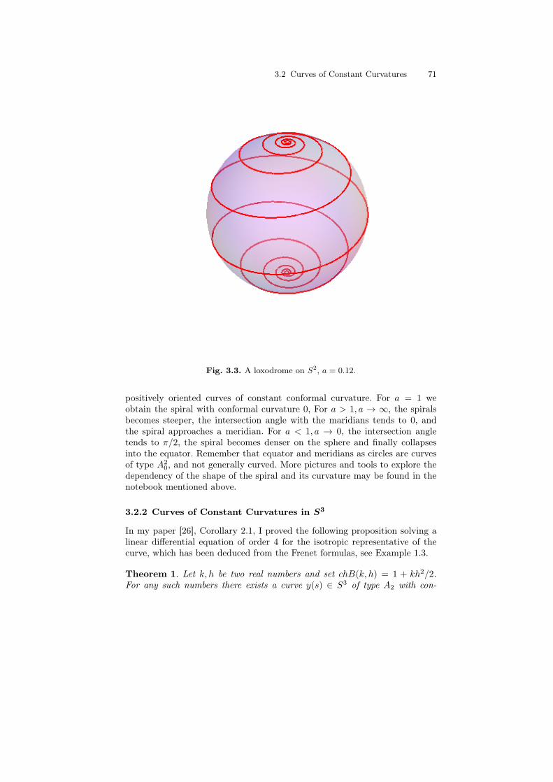
3.2 Curves of Constant Curvatures 71
Fig. 3.3. A loxodrome on S2, a = 0.12.
positively oriented curves of constant conformal curvature. For a = 1 weobtain the spiral with conformal curvature 0, For a > 1, a → ∞, the spiralsbecomes steeper, the intersection angle with the maridians tends to 0, andthe spiral approaches a meridian. For a < 1, a → 0, the intersection angletends to π/2, the spiral becomes denser on the sphere and finally collapsesinto the equator. Remember that equator and meridians as circles are curvesof type A2
0, and not generally curved. More pictures and tools to explore thedependency of the shape of the spiral and its curvature may be found in thenotebook mentioned above.
3.2.2 Curves of Constant Curvatures in S3
In my paper [26], Corollary 2.1, I proved the following proposition solving alinear differential equation of order 4 for the isotropic representative of thecurve, which has been deduced from the Frenet formulas, see Example 1.3.
Theorem 1. Let k, h be two real numbers and set chB(k, h) = 1 + kh2/2.For any such numbers there exists a curve y(s) ∈ S3 of type A2 with con-

72 3 Möbius Geometry of Curves
stant Möbius geometric curvatures k1 = k, k2 = h and natural parameters ∈ R uniquely defined up to Möbius transformations. These curves have thefollowing properties:
a) For h = 0 the curve is a loxodrome lying in a sphere S2 ⊂ S3.b) If chB(k, h) = 0 the curve is Möbius equivalent to a helix in the Eu-clidean space E3.c) If chB(k, h) > 0 and h = 0 the curve is Möbius equivalent to a curveof constant metric curvatures in the hyperbolic space E3(−c2).d) If chB(k, h) < 0 the curve is Möbius equivalent to a curve of constantmetric curvatures in the elliptic space E3(c2).
P r o o f. Here I will prove the theorem using the fact that the curves ofconstant curvatures are orbits of 1-parametric subgroups of the Möbius group,see the beginning of this section and Proposition 8 in Section 3. By the Fun-damental Theorem 3.1.10 the curves of type A2 in the Möbius space S3 forma Frenet class of curves, see Definition 2 in Section 3. The matrix of the Frenetformulas in Example 1.3 is
cc(k, h) =
0 k 1 0 01 0 0 0 k0 0 0 −h 10 0 h 0 00 1 0 0 0
, k, h ∈ R. (8)
One easily checks that the matrix cc(k, h) satisfies the equation
cc(k, h)′ · gr + gr · cc(k, h) = 0,
where gr denotes the Gram matrix (1.3.33) in isotropic-orthogonal coordi-nates. By (1.3.59) this means that cc(k, h) is an element of the Lie algebra ofthe Möbius group. By Section 3, Proposition 8, we get all curves of constantcurvatures as orbits of the 1-parametric subgroups
g[k, h](t) := exp(cc(k, h)t). (9)
It follows
Proposition 2. Let x0 = [a0] be the origin of the Möbius space S3 withrespect to a fixed isotropic orthogonal coordinate system. Then the orbitsx[k, h](t) defined by
γ[k, h](t) := g[k, h](t)x0 (10)
are curves γ[k, h] of constant curvatures k,h in the Möbius space S3, t isthe natural conformal parameter. These curves form a complete system ofrepresentatives in the class of the curves of constant curvatures of type A2.The column vectors of the matrix g[k, h](t) are the vectors of the Frenet frameof the curve γ[k, h]. In particular the first column
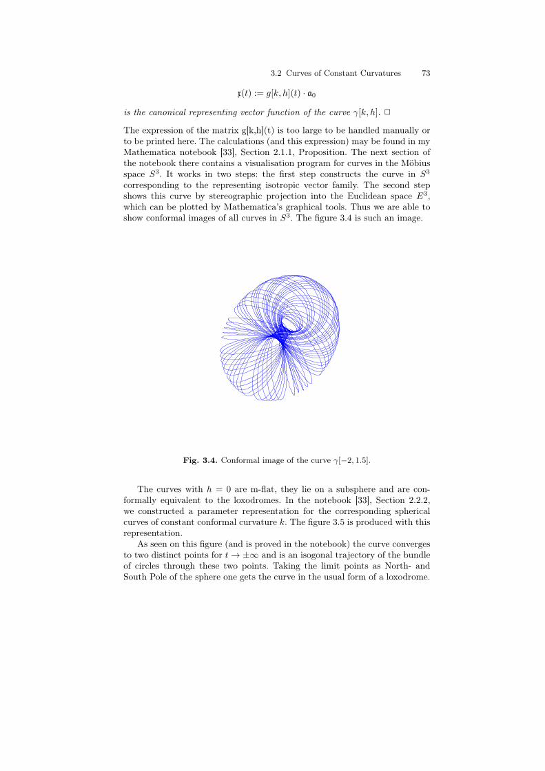
3.2 Curves of Constant Curvatures 73
x(t) := g[k, h](t) · a0
is the canonical representing vector function of the curve γ[k, h]. 2
The expression of the matrix g[k,h](t) is too large to be handled manually orto be printed here. The calculations (and this expression) may be found in myMathematica notebook [33], Section 2.1.1, Proposition. The next section ofthe notebook there contains a visualisation program for curves in the Möbiusspace S3. It works in two steps: the first step constructs the curve in S3
corresponding to the representing isotropic vector family. The second stepshows this curve by stereographic projection into the Euclidean space E3,which can be plotted by Mathematica’s graphical tools. Thus we are able toshow conformal images of all curves in S3. The figure 3.4 is such an image.
Fig. 3.4. Conformal image of the curve γ[−2, 1.5].
The curves with h = 0 are m-flat, they lie on a subsphere and are con-formally equivalent to the loxodromes. In the notebook [33], Section 2.2.2,we constructed a parameter representation for the corresponding sphericalcurves of constant conformal curvature k. The figure 3.5 is produced with thisrepresentation.
As seen on this figure (and is proved in the notebook) the curve convergesto two distinct points for t → ±∞ and is an isogonal trajectory of the bundleof circles through these two points. Taking the limit points as North- andSouth Pole of the sphere one gets the curve in the usual form of a loxodrome.

74 3 Möbius Geometry of Curves
Fig. 3.5. Conformal image of the curve γ[−5, 0].
The proof of Theorem 1 is carried out in great detail in the notebook [33].The invariant chB(k.h) is the pseudo-orthogonal scalar square of a non zerovector fixed under the action of the subgroup g[k, h](t) in the 5-dimensionalpseudo-Euclidean vector space; this vector is uniquely defined up to a constantscalar factor. In the case chB(k, h) = 0 the fixed vector is isotropic and definesa fixed point of the Möbius space whose complement gives a conformal modelof the Euclidean space, invariant under the action of the group g[k, h]. Sincethe vector and not only its direction is fixed, the group is a subgroup of theEuclidean group and the curve has metric constant curvatures: it is a helix.In case c) the fixed vector is spacelike; its orthogonal complement is a 4-dimensional pseudo-Euclidean vector space whose hypersphere of imaginaryradius is a model of the hyperbolic space invariant under the group g[k, h]. Theorbits are curves of constant curvatures in the hyperbolic geometry. Finally,in case d) a timelike vector and its orthogonal complement, a 4-dimensionalEuclidean vector space, and also its unit 3-sphere are invariant under theaction of g[k, h]. The group is a subgroup of the isometry group of the 3-sphere and the orbits are curves of constant spherical curvatures. 2
Moreover, in the notebook [33] is shown that any subgroup g[k, h] withh = 0 lies in a uniquely defined maximal abelian subgroup being 2-dimensionaland explicitly calculated. The orbits of these 2-dimensional subgroups are ho-mogeneous surfaces named Dupin cyclides. We shall classify them and describetheir properties later in the chapter about surface theory, see also my paper[27]. Any Dupin cyclide can be generated as an envelope of a 1-parametric

3.2 Curves of Constant Curvatures 75
sphere familiy (or plane family) in a twofold way. The elements of these fam-ilies are transformed into each other by the transformation of the generatingabelian subgroup, and the curves of constant curvatures are isogonal trajecto-ries of the characteristics of these envelopes being circles or lines. The simplestexample is the circular cylinder and the helices on it. The following figurescreated in [33] give examples corresponding to the cases b), c), d) in Theo-rem 1; they show a Dupin cyclide and a curve of constant curvature in eachcase.
Fig. 3.6. chB(k, h) = 0: curve γ[−0.295858, 1.3].
For t → ±∞ the two ends of the curve and the cyclide come together; thecommon limit point has the coordinates (0, 0, 1.833848). Applying a sphericalreflection with this point as center one gets a circular cylinder with a helix asthe image of figure 3.6:
Figure 3.8 shows a spherical curve of constant curvatures and figure 3.9 acurve of constant curvatures in the hyperbolic space, both embedded in thecorresponding Dupin cyclides.
Example 1. We consider a curve of constant curvature of the hyperbolictype: chB[k, h] > 0. In this case the curve tends to limit points for t → ±∞,see figure 3.9, being fixed points of the generating 1-parametric transforma-tion group. They are also limit points of the corresponding Dupin cyclide andappear as singularities of this surface, but they don’t belong to it. In the

76 3 Möbius Geometry of Curves
Fig. 3.7. Part of the spherically reflected Figure 3.6.
Fig. 3.8. chB(k, h) = −8: curve γ[−2, 1.5].
Möbius 3-sphere they are given as the points corresponding to the eigenvec-tors to real eigenvalues of the transformation. If one takes one of the fixedpoint as the infinite point and the other as origin of a conformal model of theEuclidean space, the curve appears as an isogonal trajectory of the genera-tors of a circular cone, see figure 3.10. Such curves we name 3D-spirals. Itsprojection into the x, y-plane (the plane orthogonal to the axis of the circularcone through its vertex) is a logarithmic spiral. Erecting the parallels to thez-axis on the points of the logarithmic spiral we obtain a spiral cylinder being
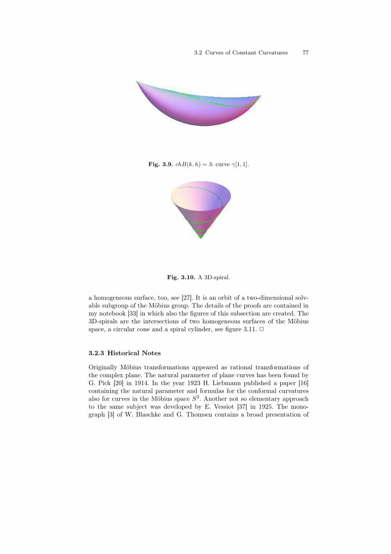
3.2 Curves of Constant Curvatures 77
Fig. 3.9. chB(k, h) = 3: curve γ[1, 1].
Fig. 3.10. A 3D-spiral.
a homogeneous surface, too, see [27]. It is an orbit of a two-dimensional solv-able subgroup of the Möbius group. The details of the proofs are contained inmy notebook [33] in which also the figures of this subsection are created. The3D-spirals are the intersections of two homogeneous surfaces of the Möbiusspace, a circular cone and a spiral cylinder, see figure 3.11. 2
3.2.3 Historical Notes
Originally Möbius transformations appeared as rational transformations ofthe complex plane. The natural parameter of plane curves has been found byG. Pick [20] in 1914. In the year 1923 H. Liebmann published a paper [16]containing the natural parameter and formulas for the conformal curvaturesalso for curves in the Möbius space S3. Another not so elementary approachto the same subject was developed by E. Vessiot [37] in 1925. The mono-graph [3] of W. Blaschke and G. Thomsen contains a broad presentation of

78 3 Möbius Geometry of Curves
Fig. 3.11. A 3D-spiral as intersection.
the geometry of plane curves (chapter 3), but only a short and incompleteoverview of some results about curves in S3 (chapter 6, § 60). A collection ofelementary results not only for curves can be found in the voluminous mono-graph of T. Takasu [35]. From another point of view, namely that of conformaltransformations of Riemannian manifolds, A. Fialkow [7] developed a confor-mal geometry of submanifolds of Riemannian spaces with tensorial methods.The natural conformal parameter which he defined is of higher order than theMöbius geometric natural parameter. In 1959 L. L. Verbitzkij [36] published ashort and precice differential geometry of curves of the n-dimensional Möbiusspace. The paper contains the invariant natural parameter and the conformalcurvatures of the curve. Our presentation in this book is a completed andcorrected version of the paper R. Sulanke [26] published 1981. A geometricinterpretation of the conformal curvatures as limits of invariants of pairs ofosculating spheres appeared in the year 2001, see A. Montesinos Amilibia,M. C. Romero Fuster, and E. Sanabria Codesal [17].
3.3 Curves in Linear Homogeneous spaces
In this section we continue the considerations of section 1.3. The Möbiusspace and the space forms introduced in Chapter 1, or more generally, allCayley-Klein spaces have the following property: they are homogeneous spacesM ∼= G/H whose defining group G is a subgroup of a real linear group.G ⊂ GL(V N ). We name such spaces linear homogeneous spaces. In the firstsubsection we consider curves in linear group spaces, and in the second weapply these considerations to calculating the curves of constant curvaturesin linear homogeneous spaces. Furthermore we describe curves of constantcurvatures in some special linear homogeneous spaces.

3.3 Curves in Linear Homogeneous spaces 79
3.3.1 Curves in Group Spaces
An advantage of the linear homogeneous spaces is that E. Cartan’s methodof moving frames can be applied in its elementary form: If z0 = (ai) denotesa fixed frame (i.e. an ordered basis) of the vector space V N , then the groupG can be realized as the subgroup of matrices (γj
i (g)) ∈ GL(N,R), definedby the coordinate representation of the moving frame
z(g) = (cj) := (g(aj)) with g(aj) = aiγij .
The structure form ω of G has the matrix representation defined by
ω = g−1dg = (ωij) = (γi
k(g))−1(dγk
j ) ∈ g ⊂ gl(N,R). (1)
Here g denotes the Lie algebra of the group G being a subalgebra of thegeneral linear Lie algebra gl(N,R) (see Example 1.3.3). Equivalently, theMaurer-Cartan forms ωi
j of G can be defined as the coefficients of the ba-sis decomposition of the differentials of the moving frame z(g) = (cj) withrespect to itself:
dcj = ciωij . (2)
Now consider a smooth function g(t) = (γij(t)) ∈ GL(N,R), t ∈ R, and set
for the components of the induced structure form
ωij(t, dt) = kij(t)dt. (3)
We obtain the derivation formulas
dcjdt
= cikij(t), (4)
a special case of which are the Frenet formulas (3.1.34). Conversely, if thereal functions kij(t) are given, equations (4) are a sytem of linear differen-tial equations for curves in the matrix space MN (R). Using the existenceand uniqueness theorem for systems of linear differential equations one easilyproves
Proposition 1. Let G ⊂ GL(N,R) be a Lie subgroup and g its Lie algebra.Given a continuous matrix function defined on the possibly infinite intervalY 1:
t ∈ Y 1 7−→ (kij(t)) ∈ MN (R)
there exists for any starting conditions cj(t0) = bj, bj ∈ V N fixed vectors, auniquely defined solution of the differential equation (4). The solutions (cj(t))are defined for all t ∈ Y 1; they are (r + 1)-times continously differentiable ifthe functions kij(t) are r-times continuously differentable. The solution g(t) =(cj(t)) belongs to the Lie group G iff the starting element (bj) belongs to Gand the coefficient matrix (kij) belongs to the Lie algebra g of G.

80 3 Möbius Geometry of Curves
P r o o f. The first and the second statement follow from the general theoryof differential equations, see e. g. E. Kamke [12] § V.19. Recursively one obtainsthe continuous differentiability of the solution deriving equation (4). For thelast statement we show first
Lemma 2. The solution (cj(t)) belongs to the general linear group GL(N,R)iff the starting value (bj) has this property. Therefore the solution either liesentirely in the general linear group, or in its complement.
P r o o f. Set h(t) := det(γij). Deriving the exterior product
c1 ∧ . . . ∧ cN = a1 ∧ . . . ∧ aNh(t),
where (aj) denotes a fixed basis of V N , one obtains the differential equationfor h(t):
dh
dt= h(t)a(t) with a(t) =
N∑0
kii(t). (5)
The solution of this equation is
h(t) = h(t0) exp(
∫ t
t0
a(t)dt),
what proves the lemma. 2If G is a Lie subgroup of GL(N,R) and X(t) := (kij(t)) belongs to its Lie
algebra g, then for any g ∈ G the element gX is tangential to G. Therefore,if the assumptions are satisfied, the starting value belongs to G and all thetangential vectors of the solution are tangential to G; thus the solution lies inG. The converse is trivial. 2
Now we consider immersions g(t) = (γij(t)) of Y 1 into the group space of
the linear Lie group G. Since G acts on itself simply transitively by the lefttranslations
La : g ∈ G 7−→ La(g) := ag ∈ G (a ∈ G),
it is a special case of a linear homogeneous space. The immersion conditionmeans that the induced structure form doesn’t have zeros on Y 1. By (1) and(3) this is equivalent to
(kij(t)) = (γil )
−1(dγl
j
dt(t)) = 0 for all t ∈ Y 1. (6)
The coefficients kij(t) we name the relative curvatures of the immersion. Theleft invariance of the structure form implies the invariance of the relativecurvatures under left translations, and Proposition 1 implies
Corollary 3. Let t ∈ Y 1 7−→ (kij(t)) = 0 be an r-times continuously differ-entiable function with values in the Lie algebra g of the linear Lie group G.

3.3 Curves in Linear Homogeneous spaces 81
Then the solutions of (4) are immersions having the properties mentioned inProposition 1. All these immersions are G-equivalent under left translations.If g(t) denotes the solution with the starting value g(t0) = e the solution withstarting value a ∈ G is given by La(g(t)). 2
We consider a parameter transformation
φ : Y 1 → Y 1, s ∈ Y 1 7→ g(s) = (cj(s)) := (cj(φ(s))) ∈ G
of the curve in G defined by the immersion g : t ∈ Y 1 7→ g(t) ∈ G. One easilycalculates: The relative curvatures of the immersion g(s) are proportional tothe relative curvatures of g(t):
dcj(s)
ds= ci(s)k
ij(s) with kij(s) = kij(φ(s))
dφ(s)
ds. (7)
Definingk(t) := (
∑i,j
(kij(t))2)1/2,
it follows that the ratioscij(t) := kij(t)/k(t)
which may be called the curvatures of the given curve in the group space G,don’t depend on the parameter representation, i.e. the immersion, representingthe curve. A parameter s is called a natural parameter if the equation k(s) = 1is satisfied for all s ∈ Y 1. Clearly, if g(t) is any immersion representing thecurve, one can find a natural parameter by integration
s(t) :=
∫ t
t0
k(t)dt = φ−1(t)
and inverting this function. From this considerations one easily proves
Proposition 4. For any curve in the group space of the linear Lie group Gthere exists a natural parameter s defined up to an addtive constant. Therelative curvatures of the immersion with the natural parameter equal the cur-vatures of the curve. An arbitrary immersion g(t) has a natural parameters = t iff for their relative curvatures the condition
k(t) = (∑i,j
(kij(t))2)1/2 = 1, (t ∈ Y 1), (8)
is satisfied. Conversely, given the curvature matrix (kij(t)) ∈ g on Y 1 satisfying(8), the solutions of (4) represent all the curves in the group space G havingt as a natural parameter and the functions kij(t) as curvatures. 2

82 3 Möbius Geometry of Curves
Thus, the curvatures define the curve up to left translations. Note that thefunctions kij(t) may not be given arbitrarily; besides of (8) the relations ensur-ing (kij(t)) ∈ g must be fulfilled. We remark that the norming of the relativecurvatures could be reached also by other conditions, e.g. if one considers aclass of curves for which the property ω1
2(t) = 0 is known for all representingimmersions, one could fix s by the condition ω1
2(s) = ds up to an additiveconstant.
The curves of constant curvature in the group space of the linear group Gcan be found easily using the matrix exponential
exp(X) :=∞∑0
Xν
ν!. (9)
The well known properties of the matrix exponential can be found in text-books of matrix calculus, or in the classical book C. Chevalley [6]. They aresummarized in the following
Proposition 5. Let G be a linear Lie group with Lie algebra g. The matrixpower series (10) converges for all X ∈ M(N,C) and has values in the generallinear group GL(N,C). The function exp has the following properties:
1. If tr(X) denotes the trace of the matrix X, one has
det(exp(X)) = exp(tr(X)). (10)
2. There exists a neighbourhood U ⊂ g of 0 ∈ g for which the restric-tion exp |U is an analytic diffeomorphism onto the neighbourhood W =expU ⊂ G of the unit element e ∈ G.
3. For commuting X,Y , [X,Y ] = 0, one has expX expY = expY expX.4. Fix an element X = 0 in g. Then the map t ∈ R 7→ exp tX ∈ G is a pa-
rameter representation of a 1-parametric subgroup of G. Any 1-parametricsubgroup of G can be obtained this way.
5. The 1-parametric subgroup corresponding to X ∈ g satisfies the differentialequation
d exp tX
dt= exp tX ·X. (11)
2
As a corollary of Proposition 5 one easily proves that the matrix expo-nential is a special case of the exponential defined in (1.3.49) for general Liegroups.
Now we compare equations (4) and (11). Considering the vectors cj ascolumn vectors of the matrix exp tX and assuming the relative curvatures asconstant, it follows
Corollary 6. Let X := (kij) ∈ g, X = 0, be constant. Then g(t) := exp tX,t ∈ R, is the solution of (4) with starting condition g(0) = e; it represents

3.3 Curves in Linear Homogeneous spaces 83
a curve of constant curvatures in the group space G. The parameter t is aconstant multiple of a natural parameter. Every curve of constant curvaturesin G is obtained by a left translation of the 1-parameter subgroup correspondingto the curvature matrix X. More exactly: All the curves of constant curvatureswith curvature matrix X = 0 are represented by immersions f(t) = ag(t) beingsolutions of (4) with starting condition f(0) = a. 2
3.3.2 Curves in Linear Homogeneous Spaces
Now let t ∈ Y 1 → x(t) ∈ Mn = Gr/Hn−r be an immersion representing acurve in the linear homogeneous space M . The immersion t ∈ Y 1 → g(t) ∈ Gis called a lift of the given immersion x(t) if
p(g(t)) = g(t)H = x(t) (t ∈ Y 1) (12)
is satisfied. With other words, the lift is nothing else as a moving frame alongthe curve.
Definition 1. A lift g(t) of the immersion is named a Frenet lift or a Frenetmoving frame, if its relative curvatures are G-invariants of the correspondingoriented curve x(t) = p(g(t)). 2
In general, Frenet lifts don’t need to exist for arbitrary curves. However inthe classical geometries for large classes of curves there exist canonically de-fined moving frames, which are special cases of Frenet frames. Their derivationequations (4) are the Frenet formula e. g. in Euclidean geometry:
Example 1. The affine group A(n) and the Euclidean group E(n) are lineargroups: one obtaines isomorphic embeddings into the general linear groupGL(n + 1,R), if in affine coordinates with respect to a fixed basis ai, i =1, . . . , n, and the fixed origin o ∈ An the affine transformation
f(C, c) : x ∈ An 7−→ f(C, c)(x) := Cx+ c ∈ An, (c ∈ Rn, C ∈ GL(n,R)),
is mapped to the matrix by
f(C, c) ∈ A(n) 7−→(1 o′
c C
)∈ GL(n+ 1,R).
The frames are here the column vectors of the matrix; the zeroth: (1, c)′ =(1, γ1, . . . γn) represents the point with coordinates (γi) in An, and the othern columns (0, cj)
′ = (0, γ1j , . . . , γ
nj )
′, j = 1, . . . , n, are a basis of the vectorspace Wn of An, Wn ⊂ V n+1 defined by γ0 = 0. For Euclidean spaces thesebases are supposed to be orthonormal; for other restrictions of affine geome-tries one has to consider the corresponding assumptions for the bases, e, g.pseudo-orthonormal or symplectic. The affine Lie algebra a(n) is representedby matrices of the shape

84 3 Möbius Geometry of Curves(0 o′
b B
)∈ a(n) ⇐⇒ b ∈ Rn and B ∈ M(n,R).
For the Euclidean Lie algebra e(n) represented in orthonormal coordinatesadditionally the skew symmetry of the matrix B must be required:(
0 o′
b B
)∈ e(n) ⇐⇒ B +B′ = 0.
We remember some basic facts of the Euclidean curve theory. A detailedexposition of the n-dimensional Euclidean curve theory may be found on myhomepage. Furthermore there one finds a Mathematica notebook [31] withmany programs for calculations of the Euclidean invariants and for graphi-cal presentations of the curves, see the section Mathematica Notebooks andComments/Euclidean Curve Theory.
Let x(s) be an immersion of Y 1 into the Euclidean space En, s its nat-ural parameter, the arc length, and (cj(s)) the canonical frame of the curve.The relative curvatures of the moving frame are given by the curvaturesk1(s), . . . , kn−1(s) for generally curved immersions as the Frenet formulas forcurves in the Euclidean space En show:
dx
ds= c1,
dc1ds
= c2k1(s),
dc2ds
= −c1k1(s) + c3k2(s),
· · · · · · · · · ,dcjds
= −cj−1kj−1(s) + cj+1kj(s),
· · · · · · · · · ,dcn−1
ds= −cn−2kn−2(s) + cnkn−1(s),
dcnds
= −cn−1kn−1(s).
The curvature matrix for the class of generally curved curves in the Euclideanspace En can not be given arbitrarily; it has the well defined shape
F (k1, . . . , kn−1) :=
0 . . . . . . . . . . . . . . . . . .1 0 k1 0 . . . . . . . . .0 −k1 0 k2 . . . . . . . . .. . . . . . . . . . . . . . . . . . . . .0 . . . . . . kj−1 0 kj . . .. . . . . . . . . . . . . . . . . . . . .0 . . . . . . . . . −kn−2 0 kn−1
0 . . . . . . . . . . . . −kn−1 0
. (13)

3.3 Curves in Linear Homogeneous spaces 85
Furthermore, for this class of curves it is well known that the curvatures satisfythe necessary conditions
kj(s) > 0 for j = 1, . . . , n− 2. (14)
The shape (13) and the conditions (14) are obtained during the adaption ofthe moving frame by E. Cartan’s or another geometrical method. Finishingthe adaption one finds a Frenet frame of the curve such that the derivationequations with (13) and (14) are satisfied. Then Proposition 1 and Corollary3 show that given the curvatures kj(s), j = 1, . . . n − 1, such that (14) issatisfied there exists one and up to Euclidean motions only one moving framehaving the curvature matrix (13); by the shape of the Frenet formulas itis clear that s is the arclength and kj(s) are the curvatures of the curvedefined by the immersion x(s) ∈ En; as a component of the moving frameit is defined uniquely up to an Euclidean motion. This is the content of theso-called Fundamental Theorem of Euclidean curve theory which states that agenerally curved curve in the n-dimensional Euclidean space is characterizedby its n− 1 curvatures as functions of the arclength. 2
Another example is the fundamental theorem in the Möbius geometry ofcurves, s. (1.34) and Theorem 1.10. This and other existence and uniquenesstheorems of differential geometry of curves show that the curvature matrixfor a given class of Frenet curves (kij(t)) is a function F (k1, k2, . . . , km) ofa complete invariant system k1, . . . , km, mostly named the curvatures of thecurve. For formulating a general fundamental theorem for curves in linearhomogeneous spaces we need
Definition 2. A Frenet class of curves in the linear homogeneous space G/His defined to be a class of curves satisfying the following conditions:
1. For any curve γ ∈ Γ is given an m-tupel of G-invariants ki(t), i = 1, . . . ,m,defined on an open interval t ∈ Y 1, and satisfying some necessary condi-tions R (see e.g. (14)).
2. There is given a matrix function F : Rm → g ⊂ M(N,R) such thatany γ ∈ Γ has a Frenet moving frame g(t) with relative curvaturesF (k1(t), . . . , km(t)), ki(t) G-invariants of γ.
3. For any m-tupel (k1, . . . , km) satisfying the conditions R the elementsF (k1(t), . . . , km(t)) do not belong to the Lie algebra h of the isotropysubgroup H.
4. Γ is closed under the action of G: with a ∈ G and γ ∈ Γ one has alsola(γ) ∈ Γ .
2
Theorem 7. Let G ⊂ GL(N,R) be a linear Lie group and g the Lie al-gebra of G. We consider a Frenet class Γ of oriented curves in the linearhomogeneous space G/H. Then for any Frenet frame of γ the parameter t is

86 3 Möbius Geometry of Curves
uniquely defined up to an additive constant, and for any m-tupel of functions(ki(t)), i = 1, . . . ,m, satisfying the necessary conditions R, there exists oneand up to a transformation la, a ∈ G, only one curve γ ∈ Γ having the givenfunctions as its curvatures. 1 For any element a ∈ G the immersion ag(t) isa Frenet lift of the immersion la(x(t)).
P r o o f. For a curve γ ∈ Γ let (kij(t)) be the matrix of the relative curva-tures of a Frenet frame g(t). We remember that equation (4) can be writtensymbolically as
dg
dt= g(t)X(t) (X(t) = (kij(t)) ∈ g). (15)
The immersion condition for the lift implies X(t) = 0. Since the kij by Defini-tion 1 of the Frenet frame are invariants of the curve (or the same constants forall γ ∈ Γ ), by (7) the only parameter transformation φ preserving them arethose with dφ/dt = 1 and the first statement follows. Now let the curvatureski(t), i = 1, . . . ,m, satisfying the conditions R be given and consider equa-tions (4) with the coefficient matrix (kij(t)) = F (k1(t), . . . , km(t)). ApplyingProposition 1 we find the corresponding immersions g(t) into the group spaceas solutions of (4). By condition 3 of Definition 2 the projections x(t) = p(g(t))are immersions into the homogeneous space G/H; indeed, the differential dpghas the kernel gh ⊂ TgG. Having in mind the uniqueness property of thesolutions g(t) and the rule
p La = la p (a ∈ G) (16)
the uniqueness of the curve up to transformations la and the last statementare proved. Since equations (4) are fulfilled for the Frenet frame g(t) of thecurve x(t), the functions ki(t) are invariants of γ characterizing the curve.2
Now we consider the curves of constant curvatures. By the general proper-ties of the solutions of (4) with constant coefficients the solutions are definedfor all t ∈ Y 1 = R. We remark first
Proposition 8. Any orbit of a 1-parameter subgroup of the Lie group G inthe homogeneous space G/H is a fixed point or a curve of constant curvatures.Conversely, any curve of constant curvatures in a Frenet class Γ of curves ina linear homogeneous space is part of an orbit of a 1-parameter subgroup ofG.
P r o o f. Let g(t) = exp(Xt) be the 1-parameter subgroup corresponding toX ∈ g. We consider the vector field on G/H generated by the action of g(t):
X(x) :=d exp(Xt)x
dt|t=0 ∈ Tx(G/H). (17)
1 In this sense one names the m-tupel (k1(t), . . . , km(t)) a complete system ofG-invariants for the curves in Γ .
3.3 Curves in Linear Homogeneous spaces 87
The zeros of this field are the fixed points of the action, and its integral curvesare the 1-dimensional orbits. Now consider an orbit x(t) = g(t)x0. Since it ishomogeneous:
x(t+ s) = g(t+ s)x0 = g(t)g(s)x0 = g(t)x(s),
all G-invariants of the orbit must be constant. Conversely, let x(t) be a pa-rameter representation of a curve γ ∈ Γ with constant curvatures k1, . . . , km.We may asssume that x(t) is defined for all t ∈ R. First we consider a curve γwhose Frenet frame z(t) has the property z(0) = e ∈ G. This Frenet frame isthe uniquely defined solution of (4) with constant coefficients F (k1, . . . , km)and starting condition z(0) = e. Fix any s ∈ R and consider the immersionw(t) := Lz(s)(z(t)) = z(s)z(t). Since the curvatures are invariant under lefttranslations and constant, w(t) is the solution of (4) with the starting condi-tion w(0) = z(s). On the other hand, the immersion t 7→ z(s+ t) has the sameproperty. By the uniqueness of the solution we obtain z(s+ t) = z(s)z(t): theFrenet frame itself is a 1-parameter subgroup2. Projecting z(t) = z(t) · e andapplying (16) one gets x(t) = lz(t)x(0) is an orbit of the subgroup z(t). For anarbitrary curve γ of constant curvatures y(t) in G/H let a = v(0) ∈ G be theelement of its Frenet frame v(t) at y(0) Then a−1v(t) is the solution (4) withstarting condition z(0) = e, and it follows a−1v(t) = z(t). The projection
y(t) = p(v(t)) = p((az(t)a−1 · a). = az(t)a−1y(0)
shows that y(t) is the orbit of a conjugated subgroup to z(t). 2Proposition 8 shows the possibility to find all curves of constant curvatures
in a linear homogeneous space: One has to find all Frenet classes of curves inthe space and in each class to solve the differential equation (4) with constantcoefficients. Since G-equivalent curves of constant curvatures correspond toconjugated 1-parameter subgroups, the classification of the curves can serveas a tool for finding the conjugacy classes of the subgroups. By the easily toprove well known formula
a · expX · a−1 = exp(Ad(a)(X)) (a ∈ G,X ∈ g) (18)
this is equivalent to the classification of the elements of the Lie algebra gunder the action of the adjoint representation of the Lie group G defined by
Ad(g)(X) := dLg dRg−1(X) (g ∈ G,X ∈ g = TeG). (19)
In the case of linear groups this amounts to the classification of the matricesX ∈ g (or linear endomorphisms of V N ) under the action of G:
Ad(g)(X) = g ·X · g−1 for G linear. (20)
Comparing Cayley-Klein Geometries we often meet the following situation:The homogeneous space Mn = G/H is an orbit Mn = Gx0 ⊂ XN = G1/H1 in2 This statement follows also from Corollary 6

88 3 Möbius Geometry of Curves
the homogeneous space XN , where G is a Lie subgroup of the larger Lie groupG1; in this case we name the transformation group [G,Mn] a subgeometry of[G1, X
N ]. Since any 1-parameter subgroup of G is also a 1-parameter subgroupof G1 it follows
Corollary 9. The curves of constant curvatures of a subgeometry G/H ofG1/H1, G ⊂ G1, are also curves of constant curvatures in the larger homoge-neous space under the canonical embedding
ι : x = gH ∈ G/H 7→ ι(x) = gH1 ∈ G1/H1, (g ∈ G).
2

References
1. M. A. Akivis and V. V. Goldberg. Conformal Differential Geometry and itsGeneralizations. John Wiley & Sons, Inc., New York etc., 1996.
2. W. Blaschke and H. Reichardt. Einführung in die Differentialgeometrie.Springer-Verlag, Berlin, Göttingen, Heidelberg, 1960.
3. W. Blaschke and G. Thomsen. Vorlesungen über Differentialgeometrie III, Dif-ferentialgeometrie der Kreise und Kugeln. Grundlehren der mat. Wiss. Bd. 29.Springer-Verlag, Berlin, 1929.
4. E. Cartan. La théorie des groupes fini et la géométrie différentielle, traitées parla méthode du repère mobile. Gauthier-Villars, Paris, 1937.
5. E. Cartan. Riemannian Geometry in Orthogonal Frames. Izd. MoskovskogoUniversiteta, Moscow, 1960. Russian. Edited by S. P. Finikov.
6. C. Chevalley. Theory of Lie Groups, volume I. Princeton University Press,Princeton, 1946.
7. A. Fialkow. The conformal theory of curves. Trans. Amer. Math. Soc., 51:435–501, 1942.
8. H. Freudenthal and H. De Vries. Linear Lie Groups. Academic Press, New York,1969.
9. S. Helgason. Differential Geometry, Lie Groups, and Symmetric Spaces. Aca-demic Press, New York, San Francisco, London, 1978.
10. Udo Hertrich-Jeromin. Introduction to Möbius Differential Geometry. LondonMath. Soc. L. N. Series 300. Cambridge University Press, Cambridge, 2003.
11. G. R. Jensen. Higher Order Contact of Submanifolds of Homogeneous Spaces,volume 610 of L. N. in Mathematics. Springer-Verlag, Berlin, Heidelberg, NewYork, 1977.
12. E. Kamke. Differentialgleichungen reeller Funktionen. Akademische Verlagsge-sellschaft Geest und Portig K.-G., Leipzig, 1952.
13. S. Kobayashi and K. Nomizu. Foundations of Differential Geometry II. Inter-science Publishers, New-York, London, 1963.
14. S. Kobayashi and K. Nomizu. Foundations of Differential Geometry I. Inter-science Publishers, New-York, London, Sydney, 1969.
15. André Lichnérowicz. Géométrie des Groupes de Transformations. Dunod, Paris,1958.
16. H. Liebmann. Beiträge zur inversionsgeometrie der kurven. Sitzungsberichteder Mathematisch-Physikalischen Klasse der Bayerischen Akademie der Wis-senschaften zu München, 53:79 – 94, 1923.

90 References
17. A. Montesinos Amilibia, M.C. Romero Fuster, and E. Sanabria Codesal. Con-formal curvatures of curves in Rn+1. Indag. Math., New Ser., 12(3):369–382,2001.
18. A. L. Onishchik and R. Sulanke. Algebra und Geometrie I. VEB DeutscherVerlag der Wissenschaften, Berlin, 1986. 2. Auflage.
19. A. L. Onishchik and R. Sulanke. Projective and Cayley-Klein Geometries.Springer-Verlag, Berlin, Heidelberg, 2006.
20. G. Pick. Zur theorie der konformen abbildung kreisförmiger bereiche. Rendicontidel Circolo Matematico di Palermo I, 37:341–344, 1914.
21. P. K. Raschewski. Riemannsche Geometrie und Tensoranalysis. VEB DeutscherVerlag der Wissenschaften, Berlin, 1959. Deutsche Übersetzung; Original:Gostechisdat, Moskau 1953; 2. Aufl. 1964.
22. Sarah E. Salvioli. On the theory of geometric objects. Journal of DifferentialGeometry, 7:257–278, 1972.
23. Ch. Schiemangk and R. Sulanke. Submanifolds of the möbius space. Math.Nachr., 96:165 – 183, 1980.
24. R. W. Sharpe. Differential Geometry, volume 166 of Graduate Texts in Mathe-marics. Springer-Verlag, New York, Berlin, Heidelberg,..., 1997.
25. R. Sulanke. On e. cartan’s method of moving frames. Colloquia Mathem. Soc.J. Bolyai. Differential Geometry, Budapest 1979, 31:681–704, 1979.
26. R. Sulanke. Submanifolds of the möbius space, ii. frenet formulas and curves ofconstant curvatures. Math. Nachrichten, 100:235–247, 1981.
27. R. Sulanke. Möbius geometry v. homogeneous surfaces in the möbius space.Coll. Math. Soc. J. Bolyai 46. Topics in Differential Geometry. Debrecen 1984,46:1141–1154, 1984.
28. R. Sulanke. Submanifolds of the möbius space iv. conformal invariants of im-mersions into spaces of constant curvature. Potsdamer Forschungen, Reihe B,43:21 – 26, 1984.
29. R. Sulanke and A. Švec. Zur differentialgeometrie der untermannigfaltigkeiteneines kleinschen raumes. Beitre zur Algebra und Geometrie, 10:63–85, 1980.
30. R. Sulanke and P. Wintgen. Differentialgeometrie und Faserbündel. VEBDeutscher Verlag der Wissenschaften, Birkhäuser, Berlin, Basel, 1972.
31. Rolf Sulanke. Euclidean Curve Theory. Mathematica Notebook, http://www-irm.mathematik.hu-berlin.de/∼sulanke/diffgeo/euklid/eucurves.tgz, 2009.
32. Rolf Sulanke. Loxodromes. Mathematica Notebook, http://www-irm.mathematik.hu-berlin.de/∼sulanke/diffgeo/moebius/loxodromes.nb, 2009.
33. Rolf Sulanke. Curves of Constant Curvatures in Möbius Ge-ometry. Mathematica Notebook, http://www-irm.mathematik.hu-berlin.de/∼sulanke/Notebooks/cccmdg.nb, 2010.
34. Rolf Sulanke. Curves in the Möbius Plane. Math-ematica Notebook, http://www-irm.mathematik.hu-berlin.de/∼sulanke/diffgeo/moebius/mdgCurves2D.nb, 2012.
35. T. Takasu. Differentialgeometrie in den Kugelräumen I. Konforme Differential-geometrie von Liouville und Möbius. Tokyo, 1938.
36. L.L. Verbitzkij. Foundations of curve theory in the n-dimensional conformalspace (russ.). Izv. Vysch. Utsch. Saved. Matematika, 6:26–37, 1959.
37. E. Vessiot. Enveloppes de sphéres et courbes gauches. J. École Polytechnique2. ser., 25:43–91, 1925.
38. Joseph A. Wolf. Spaces of Constant Curvature. University of California, Berke-ley, 1972.
Index
A⊥, 3Hn(r)
hyperbolic space, 8O(n), 18Pn, 1V n+2, 11-form of type Ad, 392nd Möbius fundamental form, 48CE(n), 6E(n), 18En
Euclidean space, 8Fc, 10G equivalent, 35G-congruent, 35G-invariant, 28, 35G,H-structure, 37J , 2Mn+2(R), 5Sn, 1Sn,m, 4TxS
n
tangent space, 4[A], 1Σm, 2ejxj
sum convention, 2⟨, ⟩, 2h(A, a, λ), 6k-flat, 513D-spiral, 76
action
left, 11adjoint representation, 29affine group, 17anticurve, 63
basisadapted to G/H, 21
basis forms, 21, 28basis point, 38
canonical lift, 45Cesàro equation, 70closed curve, 49coefficients of 1st order, 40commutator, 22conformal
geometry, 32coordinate representation, 14counterpoint, 47curvature, 81curvature
relative, 80curvature form, 33curvature tensor, 34curve, 50curve
in S2, 62in S3, 63oriented, 49regular, 49, 50
curve of type A2, 56
derivation equations, 14Dupin cyclide, 74

92 Index
Euclidean subspace, 4exponential, 24
first order reduction, 39form
canonical, 28frame
isotropic-orthonormal, 6pseudo-orthonormal, 2
frame bundle, 36frame bundle
of order 1, 40of order zero, 38
Frenetlift, 83moving frame, 83
Frenet classof curves, 85
Frenet formulas, 62, 63, 65Frenet formulas
Euclidean, 84Frenet frame, 62, 63, 65fundamental theorem
curves, 65
generally curved, 51geometric object, 35Gram matrix, 17group
affine, 16, 83conformal Euclidean, 6Euclidean, 83
homogeneous coordinates, 1homogeneous space
linear, 78
inner automorphism, 25invariants
complete system, 86isogonal, 69isotropic cone, 2isotropic subspace, 4isotropy group, 27
Jacobi identity, 22
left translation, 80Lie algebra, 22Lie algebra
Abelian, 22of a Lie group, 22
Lie grouplinear, 14
Liebmann’s formula, 59lift, 83linear isotropy representation, 27local section, 21, 37logarithmic spiral, 69loxodrome, 68, 70
Möbius curvature, 62, 63Möbius curvatures, 65Möbius geometry, 3Möbius group, 2Möbius space, 1Möbius structure, 46Möbius structure form, 46maridian, 68Maurer-Cartan forms, 15moving frame, 57, 79moving frames, 36
natural equation, 63, 70natural parameter, 58, 81negatively wound, 62normal space, 39, 41, 47, 57normal spaces
of a curve, 65normed representation, 58
oriented frames, 54origin, 10, 38osculating circles, 63osculating space, 50osculating subspheres, 51
parameter representation, 49parameter transformation, 49point
regular, 50positively wound, 62pseudo-Euclidean subspaces, 4pseudo-orthogonal group, 2
regular, 49regularity of curves, 50representation
adjoint, 23, 25, 87

Index 93
singular points, 49smooth, 49space
pseudo-Euclidean, 18space forms, 8spiral cylinder, 76structure constants, 23structure equation, 15structure equations, 20, 33structure form, 14, 23structure form
first order, 39local, 21order 0, 36, 39
subgeometry, 87
subgroupone-parametric, 24
subsphere, 2sum convention, 2
Takasu, 61tangential space, 39, 41, 47tensor field, 35translation
left, 14right, 14
umbilical point, 43
vector model, 7vertex, 63