Development of a Rig and Testing Procedures for the Experimental Investigation of

Horizontal Axis Kinetic Turbines

by

Catalina Lartiga

B.Sc., Catholic University of Chile, 2001

A Thesis Submitted in Partial Fulfilment of the

Requirements for the Degree of

MASTER OF APPLIED SCIENCES

in the Department of Mechanical Engineering

c© Catalina Lartiga, 2012

University of Victoria

All rights reserved. This thesis may not be reproduced in whole or in part, by

photocopying or other means, without the permission of the author.

ii

Development of a Rig and Testing Procedures for the Experimental Investigation of

Horizontal Axis Kinetic Turbines

by

Catalina Lartiga

B.Sc., Catholic University of Chile, 2001

Supervisory Committee

Dr. Curran Crawford., Supervisor

(Department of Mechanical Engineering)

Dr. Peter Oshkai, Departmental Member

(Department of Mechanical Engineering)

iii

Supervisory Committee

Dr. Curran Crawford., Supervisor

(Department of Mechanical Engineering)

Dr. Peter Oshkai, Departmental Member

(Department of Mechanical Engineering)

ABSTRACT

The research detailed in this thesis was focused on developing an experimental

testing system to characterize the non-dimensional performance coefficients of hor-

izontal axis kinetic turbines, including both wind turbines and tidal turbines. The

testing rig was designed for use in a water tunnel with Particle Image Velocime-

try (PIV) wake survey equipment to quantify the wake structures. Precision rotor

torque measurement and speed control was included, along with the ability to yaw

the rotor. The scale of the rotors were purposefully small, to enable rapid-prototyping

techniques to be used to produce many different test rotors at low cost to furnish a

large experimental dataset.

The first part of this work introduces the mechanical design of the testing rig

developed for measuring the output power of the scaled rotor models with considera-

tion for the requirements imposed by the PIV wake measurements. The task was to

design a rig to fit into an existing water tunnel facility with a cross sectional area of

45 by 45 cm, with a rotor support structure to minimize the flow disturbance while

allowing for yawed inflow conditions. A rig with a nominal rotor diameter of 15 cm

was designed and built. The size of the rotor was determined by studying the fluid

similarities between wind and tidal turbines, and choosing the tip speed ratio as a

scaling parameter. In order to maximize the local blade Reynolds number, and to

obtain different tip speed ratios, the rig allows a rotational speed in the range of 500

to 1500 RPM with accurate rotor angular position measurements. Rotor torque mea-

surements enable rotor mechanical power to be calculated from simulation results.

Additionally, it is included in this section a description of the instrumentation for

measurement and the data acquisition system.

iv

It was known from the outset that measurements obtained in the experiments

would be subject to error due to blockage effects inherent to bounded testing facilities.

Thus, the second part of this work was dedicated to developing a novel Computational

Fluid Dynamics (CFD) methodology to post-process the experimental data acquired.

This approach utilizes the velocity field data at the rotor plane obtained from the

water tunnel PIV test data, and CFD simulations based on the actuator disk concept

to account for blockage without the requirement for thrust data which would have

been unreliable at the low forces encountered in the tests.

Finally, the third part of this work describes the practical aspects of the laboratory

project, including a description of the operational conditions for turbine testing. A set

of preliminary measurements and results are presented, followed by conclusions and

recommendations for future work. Unfortunately, the water tunnel PIV system was

broken and thus unavailable for more than a year, so only mechanical measurements

were possible with the rig during the course of this thesis work.

v

Contents

Supervisory Committee ii

Abstract iii

Table of Contents v

List of Tables viii

List of Figures ix

Nomenclature xii

Acknowledgments xvii

Dedication xviii

1 Introduction 1

1.1 Horizontal Axis Tidal Turbines . . . . . . . . . . . . . . . . . . . . . 2

1.2 Experimental Kinetic Turbine Rotor Investigations . . . . . . . . . . 3

1.2.1 Previous Test Campaigns . . . . . . . . . . . . . . . . . . . . 4

1.2.2 Blockage effects . . . . . . . . . . . . . . . . . . . . . . . . . . 5

1.3 Motivation and Contributions . . . . . . . . . . . . . . . . . . . . . . 6

1.4 Thesis Outline . . . . . . . . . . . . . . . . . . . . . . . . . . . . . . . 8

2 Rig Design 9

2.1 Water Tunnel Facility . . . . . . . . . . . . . . . . . . . . . . . . . . . 10

2.2 Scaling Parameters . . . . . . . . . . . . . . . . . . . . . . . . . . . . 11

2.2.1 Rotor Size . . . . . . . . . . . . . . . . . . . . . . . . . . . . . 13

2.2.2 Force Estimation . . . . . . . . . . . . . . . . . . . . . . . . . 16

vi

2.3 Finite Element Method (FEM) Modelling . . . . . . . . . . . . . . . . 18

2.3.1 Failure Criteria and Maximum Deflection . . . . . . . . . . . . 18

2.3.2 Modal Analysis . . . . . . . . . . . . . . . . . . . . . . . . . . 20

2.3.3 Summary of the FEM Results . . . . . . . . . . . . . . . . . . 20

2.4 Mechanical Design . . . . . . . . . . . . . . . . . . . . . . . . . . . . 22

2.4.1 Instrument Structure . . . . . . . . . . . . . . . . . . . . . . . 24

2.4.2 Belt System . . . . . . . . . . . . . . . . . . . . . . . . . . . . 25

2.4.3 Submersed Structure . . . . . . . . . . . . . . . . . . . . . . . 28

2.4.4 The Rotor . . . . . . . . . . . . . . . . . . . . . . . . . . . . . 30

2.4.5 Yaw System . . . . . . . . . . . . . . . . . . . . . . . . . . . . 32

2.5 Instrumentation . . . . . . . . . . . . . . . . . . . . . . . . . . . . . . 33

2.5.1 The Drive System . . . . . . . . . . . . . . . . . . . . . . . . . 35

2.5.2 The Motor . . . . . . . . . . . . . . . . . . . . . . . . . . . . . 36

2.5.3 Torque cell . . . . . . . . . . . . . . . . . . . . . . . . . . . . 37

2.5.4 PIV system . . . . . . . . . . . . . . . . . . . . . . . . . . . . 39

2.5.5 DAQ Rio System . . . . . . . . . . . . . . . . . . . . . . . . . 42

3 Computational Fluid Dynamic Simulations 45

3.1 Modelling Approach . . . . . . . . . . . . . . . . . . . . . . . . . . . 46

3.1.1 Porous disk . . . . . . . . . . . . . . . . . . . . . . . . . . . . 46

3.1.2 Domain . . . . . . . . . . . . . . . . . . . . . . . . . . . . . . 46

3.1.3 Boundary Conditions . . . . . . . . . . . . . . . . . . . . . . . 48

3.2 Computational Model . . . . . . . . . . . . . . . . . . . . . . . . . . 49

3.2.1 Governing Equations . . . . . . . . . . . . . . . . . . . . . . . 49

3.2.2 Momentum Source Sink . . . . . . . . . . . . . . . . . . . . . 51

3.2.3 CFX Boundary Conditions . . . . . . . . . . . . . . . . . . . . 52

3.3 CFD Simulation Results . . . . . . . . . . . . . . . . . . . . . . . . . 53

3.3.1 Unbounded Flow Validation . . . . . . . . . . . . . . . . . . . 54

3.3.2 Bounded Flow Results . . . . . . . . . . . . . . . . . . . . . . 56

3.3.3 Tunnel Wall Boundary Growth Effects . . . . . . . . . . . . . 57

3.3.4 Reynolds Dependency Analysis . . . . . . . . . . . . . . . . . 59

4 Tunnel Blockage Correction Models 62

4.1 Thrust Based Analytical Models . . . . . . . . . . . . . . . . . . . . . 63

4.1.1 Momentum Based Model . . . . . . . . . . . . . . . . . . . . . 64

vii

4.2 Blockage Correction Model Development . . . . . . . . . . . . . . . . 66

4.2.1 CFD Correction Factors . . . . . . . . . . . . . . . . . . . . . 69

5 Experimental Procedures and Testing Campaigns 73

5.1 Objectives of the experiment . . . . . . . . . . . . . . . . . . . . . . . 74

5.1.1 Power output . . . . . . . . . . . . . . . . . . . . . . . . . . . 74

5.2 Experiment Protocol . . . . . . . . . . . . . . . . . . . . . . . . . . . 75

5.3 Experimental Blade Sets . . . . . . . . . . . . . . . . . . . . . . . . . 76

5.4 Measurement Error Estimation . . . . . . . . . . . . . . . . . . . . . 77

5.4.1 Error estimation . . . . . . . . . . . . . . . . . . . . . . . . . 78

5.5 Initial Testing Campaign . . . . . . . . . . . . . . . . . . . . . . . . . 80

5.6 Second Testing Campaign . . . . . . . . . . . . . . . . . . . . . . . . 81

5.6.1 Operational Conditions . . . . . . . . . . . . . . . . . . . . . . 82

5.6.2 Experimental Results . . . . . . . . . . . . . . . . . . . . . . . 83

5.6.3 Surface Roughness and Reynolds Number Effects . . . . . . . 84

5.6.4 Estimation of Blockage Effects . . . . . . . . . . . . . . . . . . 86

6 Conclusions 92

6.1 Rig Design . . . . . . . . . . . . . . . . . . . . . . . . . . . . . . . . . 92

6.2 Computational Fluid Dynamic Simulations . . . . . . . . . . . . . . . 93

6.3 Experimental Study . . . . . . . . . . . . . . . . . . . . . . . . . . . . 93

6.4 Future Work . . . . . . . . . . . . . . . . . . . . . . . . . . . . . . . . 94

Bibliography 95

A Momentum Theory: The Actuator Disc Concept 100

B Finite Element Analysis Modelling 105

B.1 Geometry and Material Properties . . . . . . . . . . . . . . . . . . . . 105

B.2 Forces Applied to the System . . . . . . . . . . . . . . . . . . . . . . 108

B.3 Maximum Deflection - Results . . . . . . . . . . . . . . . . . . . . . . 109

B.4 Modal Analysis - Results . . . . . . . . . . . . . . . . . . . . . . . . . 110

B.5 Mesh Refinement . . . . . . . . . . . . . . . . . . . . . . . . . . . . . 110

C PIV Theory 113

viii

List of Tables

Table 2.1 Full size tidal turbine versus scaled model . . . . . . . . . . . 15

Table 2.2 Forces at the rotor plane . . . . . . . . . . . . . . . . . . . . 17

Table 2.3 Dimensions resulting from FEM analysis . . . . . . . . . . . . 22

Table 2.4 Characteristics of the candidate belts . . . . . . . . . . . . . 28

Table 3.1 ∆ CP (%) with respect theory value for different disc thickness 55

Table 3.2 Cases for mesh dependency study . . . . . . . . . . . . . . . 56

Table 3.3 ∆ CP (%) with respect theory value for different mesh config-

urations . . . . . . . . . . . . . . . . . . . . . . . . . . . . . 56

Table 3.4 Maximum CP values . . . . . . . . . . . . . . . . . . . . . . . 58

Table 3.5 Turbine size and flow conditions for additional RANS simula-

tions . . . . . . . . . . . . . . . . . . . . . . . . . . . . . . . 60

Table 5.1 Pumping system frequencies and tunnel inflow velocity . . . 76

Table 5.2 Uncertainties of measurement . . . . . . . . . . . . . . . . . 79

Table 5.3 Pumping system frequencies and tunnel inflow velocity . . . 83

Table B.1 Configurations of study for modal analysis . . . . . . . . . . 106

Table B.2 Maximum deflections and stresses (Non-yawed condition) . . 110

Table B.3 Max.deflections and stresses at 30 yaw angle . . . . . . . . . 110

Table B.4 Maximum deflections and stresses at 45 yaw angle . . . . . . 111

Table B.5 Result of modal analysis - natural frequencies [Hz] . . . . . . 111

ix

List of Figures

Figure 1.1 Tidal Turbine Industry . . . . . . . . . . . . . . . . . . . . . 3

(a) Tidal Generation Ltd . . . . . . . . . . . . . . . . . . . . . . . . 3

(b) Marine Current . . . . . . . . . . . . . . . . . . . . . . . . . . . 3

(c) Lunar Energy . . . . . . . . . . . . . . . . . . . . . . . . . . . . 3

Figure 1.2 Actuator disk concept in open and bounded flows . . . . . . 6

(a) Unbounded domain . . . . . . . . . . . . . . . . . . . . . . . . . 6

(b) Bounded domain (e.g. water tunnel) . . . . . . . . . . . . . . . 6

Figure 2.1 Water tunnel facility . . . . . . . . . . . . . . . . . . . . . . 10

Figure 2.2 The energy extracting stream-tube of a wind turbine (adapted

from [1]) . . . . . . . . . . . . . . . . . . . . . . . . . . . . . 14

Figure 2.3 Schematic of the testing rig . . . . . . . . . . . . . . . . . . . 19

Figure 2.4 FEM tube model of the testing rig . . . . . . . . . . . . . . . 21

Figure 2.5 Schematic operation . . . . . . . . . . . . . . . . . . . . . . . 24

Figure 2.6 Key components of the rig . . . . . . . . . . . . . . . . . . . 25

Figure 2.7 Components of the instrument structure . . . . . . . . . . . . 26

Figure 2.8 Rig for belt testing . . . . . . . . . . . . . . . . . . . . . . . 27

Figure 2.9 Submerged support structure . . . . . . . . . . . . . . . . . . 29

Figure 2.10 Model of fairings covering the submerged structure . . . . . . 30

Figure 2.11 Rotor assembly . . . . . . . . . . . . . . . . . . . . . . . . . 31

Figure 2.12 Yaw system operation . . . . . . . . . . . . . . . . . . . . . . 33

Figure 2.13 PIV system layout . . . . . . . . . . . . . . . . . . . . . . . . 34

Figure 2.14 Experiment system schematic . . . . . . . . . . . . . . . . . 36

Figure 2.15 Drive system . . . . . . . . . . . . . . . . . . . . . . . . . . . 37

Figure 2.16 Performance curve Parker Motor HV233 . . . . . . . . . . . . 38

Figure 2.17 Novatech installation schematic . . . . . . . . . . . . . . . . 39

Figure 2.18 General schematics of PIV system . . . . . . . . . . . . . . . 40

x

Figure 2.19 CompactRio package . . . . . . . . . . . . . . . . . . . . . . 43

Figure 2.20 LabView interface . . . . . . . . . . . . . . . . . . . . . . . . 44

Figure 3.1 Quarter domain water tunnel model (ANSYS CFX) . . . . . 47

Figure 3.2 CFX quarter domain boundary conditions . . . . . . . . . . . 52

Figure 3.3 CP v/s CT for turbulent flow conditions in bounded domain

with opening boundary conditions . . . . . . . . . . . . . . . 54

Figure 3.4 CP v/s CT for turbulent flow conditions in water tunnel domain 57

Figure 3.5 CP values for a wider range of Thrust Coefficients . . . . . . 58

Figure 3.6 Boundary layer effect for a rotor diameter 15 mm (9% blockage

ratio) referenced to tunnel conditions . . . . . . . . . . . . . 59

Figure 3.7 CP v/s CT , Unbounded domain . . . . . . . . . . . . . . . . 61

Figure 3.8 CP increment v/s blockage ratio at CT = 8/9 . . . . . . . . . 61

Figure 4.1 Actuator disk model in a closed tunnel section . . . . . . . . 65

Figure 4.2 Trend of CP v/s CT in water tunnel and unbounded domains 67

Figure 4.3 CFD-computed corrected velocity to inlet velocity ratio for

different blockage ratios and operational conditions . . . . . . 69

Figure 4.4 Comparison between analytical and CFD power coefficient

corrections (all values corrected to free-stream, CT referred

to tunnel conditions) . . . . . . . . . . . . . . . . . . . . . . 71

Figure 4.5 Correction curve for the experimental testing referenced to

tunnel conditions . . . . . . . . . . . . . . . . . . . . . . . . 72

(a) Ratio of corrected velocity to tunnel velocity v/s axial induction

factor for a 9% blockage ratio . . . . . . . . . . . . . . . . . . . 72

(b) Increment in power coefficient v/s axial induction factor for a 9%

blockage ratio . . . . . . . . . . . . . . . . . . . . . . . . . . . . 72

Figure 5.1 Frictional Torque - Dec. 2010 . . . . . . . . . . . . . . . . . . 80

Figure 5.2 CP v/s λ Results Dec. 2010 . . . . . . . . . . . . . . . . . . 81

Figure 5.3 α (deg) v/s r/R . . . . . . . . . . . . . . . . . . . . . . . . . 83

Figure 5.4 Re v/s r/R . . . . . . . . . . . . . . . . . . . . . . . . . . . . 84

Figure 5.5 CP v/s λ at low water tunnel velocity (rough) . . . . . . . . 85

Figure 5.6 CP v/s λ at high water tunnel velocity (rough) . . . . . . . . 86

Figure 5.7 CP v/s λ at high water tunnel velocity (smooth) . . . . . . . 87

xi

Figure 5.8 CP v/s λ at high water tunnel velocity, 1.0X and 1.5X smooth

blades . . . . . . . . . . . . . . . . . . . . . . . . . . . . . . . 88

Figure 5.9 CL v/s α, forced transition at 0.1 chord . . . . . . . . . . . . 88

Figure 5.10 CL v/s α, forced transition at 0.3 chord . . . . . . . . . . . . 89

Figure 5.11 CD v/s CL xtr=0.1 . . . . . . . . . . . . . . . . . . . . . . . 89

Figure 5.12 CD v/s CL xtr=0.3 . . . . . . . . . . . . . . . . . . . . . . . 90

Figure 5.13 CP v/s λ 1X rough surface blade - correction bounds . . . . 90

Figure 5.14 CP v/s λ 1X smooth surface blade - correction bounds . . . . 91

Figure 5.15 CP v/s λ 1.5X rough surface blade - correction bounds . . . . 91

Figure A.1 An energy extracting actuator disk and stream-tube (adapted

from the Wind Energy Handbook [1]) . . . . . . . . . . . . . 101

Figure B.1 Rig structure modelling . . . . . . . . . . . . . . . . . . . . . 107

Figure B.2 Rig structure modelling . . . . . . . . . . . . . . . . . . . . . 108

Figure B.3 Mesh analysis (Model10) . . . . . . . . . . . . . . . . . . . . 112

Figure C.1 Numerical processing flow-chart DPIV . . . . . . . . . . . . . 115

xii

Nomenclature

Chapter 1

V ′ Glauert’s equivalent axial freestream velocity

UF Bahaj’s equivalent open speed

Pwt Power in the water tunnel domain

Punb Power in the unbounded domain

C Cross sectional area of the water tunnel

W Cross sectional area at the far wake

ui Axial velocity at location i

pi Pressure at location i

UC Corrected axial velocity to free stream conditions

CT,wt Thrust coefficient characteristic of water tunnel domain

CT,unb Thrust coefficient characteristic of unbounded domain

CP,wt Power coefficient characteristic of water tunnel domain

CP,unb Power coefficient characteristic of unbounded domain

y+ Non-dimensional wall distance

xiii

Chapter 2

CP Power coefficient

λ Tip speed ratio

ρ Water density

Ω Angular velocity

P Power

R Radius of the Rotor

U∞ Axial velocity of the undisturbed free stream

U Stream velocity

U0 Axial inflow velocity in the water tunnel

Rw Radius of the wake expansion

a Axial induction factor

Re Reynolds Number

A Cross sectional area at the disc

T Thrust force

γ Angle of Yaw

FX Maximum Thrust force aligned to the axis of the turbine

FZ Maximum Thrust force orthogonal to the axis of the turbine

σVM Von Mises stress

σi Stress in the i direction

[K] Stiffness matrix

θi Mode shape vector

[M ] Mass matrix

ω2i Eigenvalue i

ΩEi Natural frequency of a structure of mode i

L Characteristic length

c Chord length

D Rotor disc diameter

Rec Reynolds Number based on chord length

ReD Reynolds Number based on rotor diameter length

Tfrictional Frictional torque

Thydro Hydrodynamic torque

Treact Reaction torque

xiv

Chapter 3

χ Momentum sink

CT Thrust coefficient

U0 Axial inflow velocity in the water tunnel

ρ Water density

t Thickness of the disc

D Diameter of the scaled rotor

K − Ω Equation to model turbulence

Re Reynolds Number

u vector velocity

p pressure

τ stress tensor

(SM) External momentum sources

u Turbulent Vector velocity

u Mean velocity

u′ Random velocity fluctuation

K CFX Momentum Source Coefficient

UZ Velocity in the Z axis

US Flow speed in the streamwise direction

popening Pressure at the Opening boundary surface

pspec Pressure specified at certain surface

Un,wall Velocity normal to the wall

τw Shear stress

Uinlet Velocity specified at inlet surface

Uspec,X X axis velocity component specified at inlet

Uspec,Y Y axis velocity component specified at inlet

Uspec,Z Z axis velocity component specified at inlet

paverage,outlet Average pressure over the outlet surface

Uwall Vector velocity at the wall surface

CP Power coefficient

CT Thrust coefficient

a Axial induction factor

y+ Non-dimensional wall distance

Atunnel Water tunnel cross sectional area

xv

Chapter 4

CP Power coefficient

CT Thrust coefficient

a Axial induction factor

V ′ Glauert’s equivalent axial freestream velocity

U0 Axial inflow velocity in the water tunnel

UC Corrected axial velocity to free stream conditions

UF Bahaj’s equivalent open speed

ui Axial velocity at location i

pi Pressure at location i

CP,unb Power coefficient characteristic of unbounded domain

CP,wt Power coefficient characteristic of water tunnel domain

CT,unb Thrust coefficient characteristic of unbounded domain

CT,wt Thrust coefficient characteristic of water tunnel domain

Pwt Power in the water tunnel domain

Punb Power in the unbounded domain

C Cross sectional area of the water tunnel

W Cross sectional area at the far wake

Ucorr CFD corrected axial velocity

K CFX Momentum Source Coefficient

xvi

Chapter 5

Pwt Power in the water tunnel domain

τrotor Measured reaction torque

Ω Angular velocity

CP,wt Power coefficient in water tunnel before correction

ρ Water density

U∞ Axial velocity of the undisturbed free stream

R Radius of the Rotor

λ Tip speed ratio

α Angle of attack

CL Lift coefficient

CD Drag coefficient

r Local position along blade

UNC.RX Random uncertainty estimation of X measurement

SX Standard deviation of the sample X

M Sample size

UNC Total uncertainty estimates

xvii

ACKNOWLEDGEMENTS

I wish to thank all those who helped me to complete this project and turned this

graduate time into a great experience. Without their support this work may not have

been possible.

My sincere gratitude to my supervisor Dr. Curran Crawford, for his patience,

support, and guidance through all the stages in this learning process. I really ap-

preciate the time Dr. Crawford spent helping me to develop understanding of my

subject of study and helping me to solve practical aspects of my work. I would like

to extend my thanks to Rodney Katz, Oleksandr Barannyk, and Patrick Chang for

their advice and hands-on help with the practical execution of my experiment; and

Heshan Fernando for his work on the rig design.

And last but not least, my deepest gratitude goes to my family and Patricio, for

their love and support over all these years.

xviii

DEDICATION

To Patricio, for his vision and his encouragement through this journey

Chapter 1

Introduction

As a result of the Kyoto Protocol and the Copenhagen International Conference on

Climate Change, several industrialized countries have committed to reduce Green

House Gas (GHG) emissions and to increase electricity generation using low-carbon

intensive technologies. Consequently, emerging economies have recognized the poten-

tial role of renewable energies within a portfolio of electric power generation projects.

Research on renewable energy technologies has become a priority in order to develop a

cost-competitive green technology capable of providing reliable and predictable access

to energy, and allowing countries to reach their GHG reduction targets.

In this context, kinetic turbines, as mechanical energy extracting devices, are a

choice for environmentally-friendly production of alternative energy in the near future.

Wind turbines, tidal turbines and in-stream turbines are the key devices being devel-

oped. Although wind turbines are considered a mature technology, already installed

in several locations and providing energy to the grid, there is still much research being

carried out to better understand the wakes of single devices and turbine arrays. Many

studies on blade profiles have been carried out in the aeronautic industry, however

to fully understand how blade geometry affects the flow downstream of the rotor, in

turn affecting the turbine performance, experimental studies on vortex wakes have

been recently performed [2]. A comprehensive summary of several experiments done

and numerical studies performed on wind turbines for both near and far wakes is

presented by Vermeer and Sorensen [3].

Regarding marine turbines, not much has been established as standard design yet

in the industry. The present designs for marine turbines are basically an adaption

of conventional wind turbines, taking into account the inherent differences of devices

2

harnessing the kinetic energy of marine currents instead of air. Comprehensive studies

and experiments are required in order to secure and strengthen the application of this

technology. As wind turbines are more familiar to the reader, a presentation of tidal

turbine technology is presented next, although the experimental rig and techniques

developed in this thesis are applicable to all forms of kinetic turbine testing.

1.1 Horizontal Axis Tidal Turbines

Energy from marine currents seems to be a reliable and perhaps more importantly

a predictable source of electricity generation [4]. The typical resource referred when

talking about marine turbines are the tides, caused by the gravitational forcing of

the sun and moon on the oceans. Two other water-based kinetic turbine applications

also exist: run-of-river turbines in freely flowing rivers, and ocean-based turbines

set in ocean flows largely driven by wind stress, such as the Gulf Stream, or ocean

circulation driven by surface heat and freshwater fluxes. In all cases, water-based

kinetic turbines offer a higher power density than other types of renewable sources

(such as wind). Since it is possible to identify the sites where sea flows are channelled

due to topographies, it makes possible to locally study the source itself in order to

better predict the energy output.

Since the design of Horizontal Axis Tidal Turbines (HATTs) is an emerging area,

and even if the majority of these devices present a conventional design setting a rotat-

ing shaft in line with the flowstream, it is possible to find as many different types of

turbines as companies getting into the market. HATTs development has widely ben-

efited from the wind industry and their experience with axial rotor machines. In the

same way, several companies with tidal stream technologies under development have

been strongly influenced by the predominantly open three-bladed rotor design. Other

companies have moved to in-stream turbines, taking advantages of flow acceleration

[5].

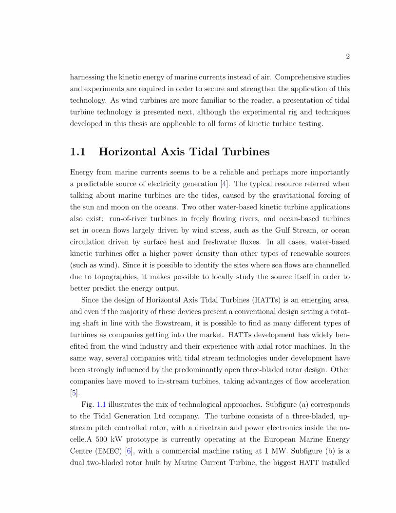
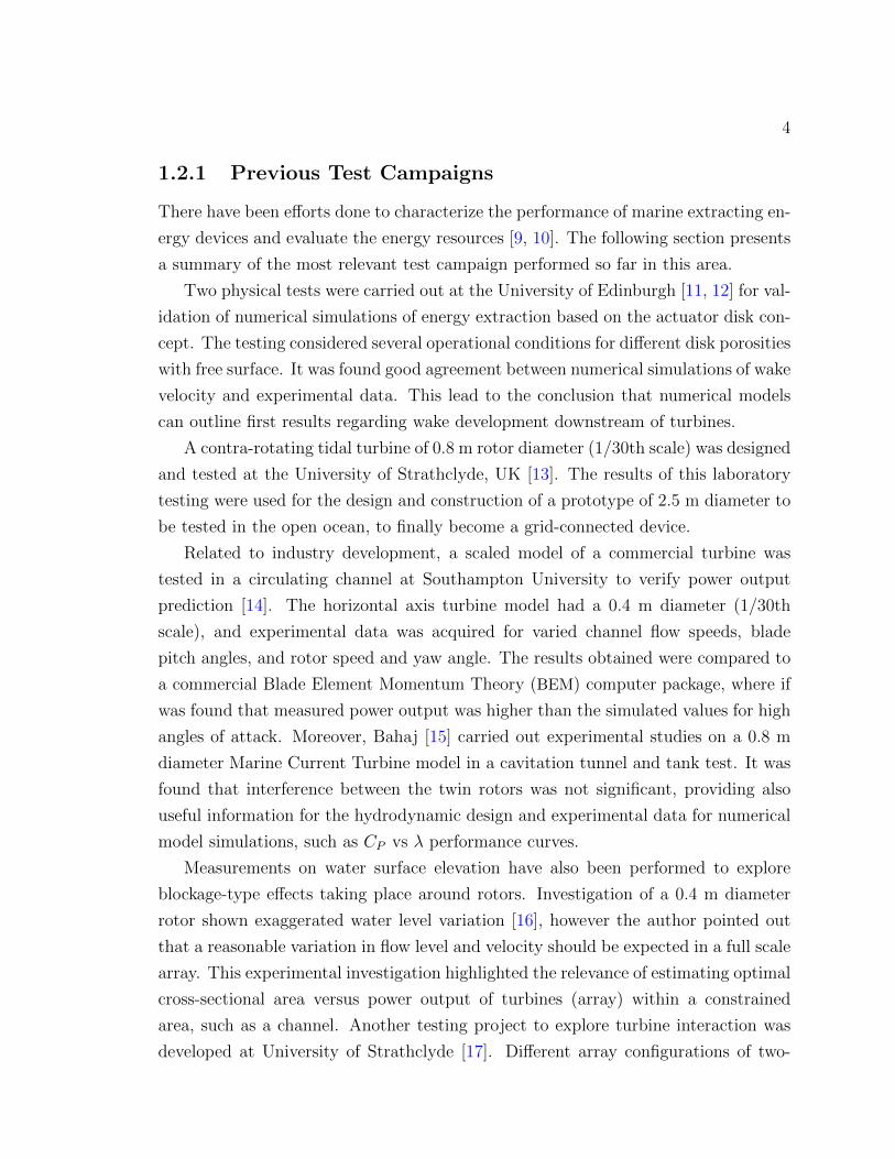
Fig. 1.1 illustrates the mix of technological approaches. Subfigure (a) corresponds

to the Tidal Generation Ltd company. The turbine consists of a three-bladed, up-

stream pitch controlled rotor, with a drivetrain and power electronics inside the na-

celle.A 500 kW prototype is currently operating at the European Marine Energy

Centre (EMEC) [6], with a commercial machine rating at 1 MW. Subfigure (b) is a

dual two-bladed rotor built by Marine Current Turbine, the biggest HATT installed

3

in the ocean (Strangford Narrow), generating 1.2 MW. Finally, subfigure (c) displays

the Lunar Energy ducted turbine. Ducted turbines have smaller rotor diameters and

a shroud that accelerates the incoming flow, with a 500 kW prototype not yet tested

in ocean, and a 1 MW device under development [5]. Not shown in figure, Nova

Scotia Power has installed a 1 MW in-stream tidal turbine in Minas Passage of the

Bay Fundy, to explore the feasibility of harnessing tidal energy on a commercial scale

[7].

(a) Tidal Generation Ltd (b) Marine Current (c) Lunar Energy

Figure 1.1: Tidal Turbine Industry

1.2 Experimental Kinetic Turbine Rotor Investi-

gations

An important amount of knowledge from wind turbines and classical marine propellers

can be applied to the design and operational analysis of marine turbines [1, 8]. How-

ever, relevant differences inherent to flow characteristic and fluid properties of marine

turbines, such as density, high Reynolds number, viscosity, turbulence, cavitation, etc,

must be taken into account in the development processes of these machines. Contin-

ued experimental investigation is required to validate prediction codes and designs in

this field, as well as that of wind turbines, for which experimental data is also sparse.

4

1.2.1 Previous Test Campaigns

There have been efforts done to characterize the performance of marine extracting en-

ergy devices and evaluate the energy resources [9, 10]. The following section presents

a summary of the most relevant test campaign performed so far in this area.

Two physical tests were carried out at the University of Edinburgh [11, 12] for val-

idation of numerical simulations of energy extraction based on the actuator disk con-

cept. The testing considered several operational conditions for different disk porosities

with free surface. It was found good agreement between numerical simulations of wake

velocity and experimental data. This lead to the conclusion that numerical models

can outline first results regarding wake development downstream of turbines.

A contra-rotating tidal turbine of 0.8 m rotor diameter (1/30th scale) was designed

and tested at the University of Strathclyde, UK [13]. The results of this laboratory

testing were used for the design and construction of a prototype of 2.5 m diameter to

be tested in the open ocean, to finally become a grid-connected device.

Related to industry development, a scaled model of a commercial turbine was

tested in a circulating channel at Southampton University to verify power output

prediction [14]. The horizontal axis turbine model had a 0.4 m diameter (1/30th

scale), and experimental data was acquired for varied channel flow speeds, blade

pitch angles, and rotor speed and yaw angle. The results obtained were compared to

a commercial Blade Element Momentum Theory (BEM) computer package, where if

was found that measured power output was higher than the simulated values for high

angles of attack. Moreover, Bahaj [15] carried out experimental studies on a 0.8 m

diameter Marine Current Turbine model in a cavitation tunnel and tank test. It was

found that interference between the twin rotors was not significant, providing also

useful information for the hydrodynamic design and experimental data for numerical

model simulations, such as CP vs λ performance curves.

Measurements on water surface elevation have also been performed to explore

blockage-type effects taking place around rotors. Investigation of a 0.4 m diameter

rotor shown exaggerated water level variation [16], however the author pointed out

that a reasonable variation in flow level and velocity should be expected in a full scale

array. This experimental investigation highlighted the relevance of estimating optimal

cross-sectional area versus power output of turbines (array) within a constrained

area, such as a channel. Another testing project to explore turbine interaction was

developed at University of Strathclyde [17]. Different array configurations of two-

5

bladed rotors of 25 cm diameter were tested at a towing tank having a maximum

velocity of 0.47 m/s. A significant power output reduction was found for in-line

turbine arrays, however an optimal array configuration was found that optimized

energy production, heading for an array efficiency of 100 %.

At this point, we can recognize that more experimental data is needed to validate

designs and simulations for emerging HATT. All types of kinetic turbine designs

(including wind turbines) can benefit from experimental studies.

1.2.2 Blockage effects

A common issue that arises in this type of experimental testing is that Reynolds

similitude is improved with larger scale models. Fortuitously, the behaviour of rotor

wake vorticity is relatively insensitive to Reynolds number [3]. However, for a larger

ratio of the rotor swept area to the tunnel section area, the greater the associated error

due to blockage. Consequently, larger models less accurately predict the performance

of the full scale turbine. Physically, the walls of the water tunnel constrain the

flow and cause an increment in the velocity around the rotor, compared to the inlet

velocity.

A simple model of the turbine takes the rotor as a thin disc plane that extracts

energy from the stream as the flow passes through it. This approach is known as

the actuator disc concept, and is explained in Appendix A. The energy extraction

done by the turbine implies a drop in static pressure in the area right after the disc

plane, which downstream causes a reduction in the velocity and cross sectional area

expansion of the streamtube through the rotor.

This situation is depicted in Fig. 1.2a, if the turbine is placed in an unbounded

domain. It is assumed that flow at constant pressure p0 surrounds the stream-tube

and the flow velocity remains undisturbed U0 everywhere outside the stream-tube

surrounding the disk. Conversely, if the turbine is placed in a constrained domain,

such as in a water tunnel section as shown in Fig. 1.2b, there is a change in the

velocity and pressure that surround the stream-tube compared to the far upstream

(undisturbed) conditions. This effect leads to higher forces and power outputs mea-

sured in the bounded domain relative to unbounded flow conditions around the real

machine. Conversely to propeller testing which create contracting wakes, this block-

6

Undisturbed

Velocity (Uo)

Unbounded domain

Uo Uo po

Wake velocity << UoUo

po

Velocity

across the

disc < Uo

Disc Far downstreamFar Upstream

(a) Unbounded domain

Water tunnel section

Undisturbed

Velocity (Uo)

Velocity > Uo Velocity > Uo

Uo

po

Pressure ≠ po

Wake velocity << UoVelocity

across the

disc < Uo

Disc

Pressure ≠ po

Far Upstream Far downstream

(b) Bounded domain (e.g. water tunnel)

Figure 1.2: Actuator disk concept in open and bounded flows

age is not negligible for kinetic turbines which extract energy from the flow and cause

flow expansion in the wake behind the rotor.

In the past decades, several efforts have been made to provide a suitable method-

ology to correct for wind and water tunnel blockage effects [18–20]. To date, these

methods have been based on the axial momentum theory representing this tunnel

interference by an equivalent free stream velocity. Analytical expressions correlating

this equivalent open flow velocity to thrust coefficient are used to correct the charac-

teristic power coefficient, and consequently real power output [15, 18–21]. However,

the validity of these analytic corrections as the blockage ratio, the turbulence level,

and rotor loads increase, has not been clearly defined. These factors might affect

the flow field in the water tunnel used in the current work in such a way that the

assumptions from which the analytical corrections were derived are not longer valid.

Additionally, the need for a new post processing methodology arises when thrust data

is not available in the experimental testing. In the current work, due to the small

size of the rotors, it is impractical to measure with any accuracy the thrust force of

the rotor itself.

1.3 Motivation and Contributions

The purpose of this thesis research was to build a rig and develop associated testing

methods for the physical testing of scaled models of kinetic turbines in an existing

7

water tunnel facility. The experimental information generated by the testing could

then be used for turbine performance assessment, rotor design efforts, and validation

of numerical prediction codes. The rig was intentionally designed for small rotors,

so that many blade sets could quickly be produced using Fused Deposition Modeling

(FDM), a rapid prototyping technique producing Acrylonitrile-Butadiene-Stryrene

(ABS) or polycarbonate parts in 3D, thereby allowing the testing of a wide range of

rotors to produce a rich set of data. Any scaled model has limitations due to the scaled

physics of the facilities and rig, as well as the attainable accuracy of the instruments

used for measurement. This project therefore focused specifically on developing a

precision testing rig with the capability to properly scale operational conditions of

real machines.

The experimental study described in this work includes the use of Particle Image

Velocimetry (PIV) techniques to obtain quantitative information about the vector flow

field at the rotor plane and upstream/downstream. Flow measurements are obtained

at various rotor azimuthal positions at the same time that power measurement are

taken. The intention is to use this information in future studies in order to validate

potential flow and Computational Fluid Dynamics (CFD) simulations that resolve

wake features.

It is important to note that accurate thrust force measurements are not possible for

the size of the scale model built. Since PIV data will be available from the experiment

anyway, a novel actuator-disk CFD-PIV methodology was developed to post-process

the measured experimental data to properly account for tunnel blockage effects in the

absence of thrust measurements [22, 23].

Although not detailed in this thesis, the CFD simulation modelling approach was

also applied to a study [24] looking at recommended testing procedures for full-scale

turbines in-situ. In particular, the study looked at blockage effects in comparison be-

tween various modelling approaches including complete CFD with explicit resolution

of the blades. Recommendations were supplied to the authors of tidal turbine testing

standards currently in development related to acceptable testing parameters to avoid

erroneous performance estimates through testing in constrained conditions.

Unfortunately, the water tunnel PIV equipment was broken for an extended pe-

riod covering the entire latter half of the thesis period, and therefore only an initial

mechanical measurement test campaign can be presented in this thesis as an initial

application of the rig. Progress was also delayed by a broken torque transducer which

8

had to be returned to the UK for servicing after a difficult fault-diagnosis process.

In addition, a problem with the driving stepper motor causing pull-out and severe

vibration that was only finally resolved by replacing the motor.

1.4 Thesis Outline

This thesis consist of five chapters, organized as follows. Chapter 2 details the me-

chanical design of the rig focused on ensuring accurate measurements could be taken

with the forces involved, and that PIV data could be gathered through a range of

operating conditions. Chapter 3 presents the CFD simulations used to study rotor

behaviour in unbounded and bounded domains, leading to the work presented in

Chapter 4 carried out to deal with tunnel blockage effects. Chapter 5 then presents

the initial experimental campaigns carried out to test the operation of the rig, in

the absence of PIV measurements due to protracted equipment breakdown. Finally,

Chapter 6 summaries the work and provides direction for follow-on use of the rig once

the PIV system is operational.

9

Chapter 2

Rig Design

This chapter describes the main aspects that were involved in the mechanical design

of an experimental apparatus for the investigation of the hydrodynamic performance

of kinetic turbines. The rig was initially developed with a view to testing HATT. The

model parameters were therefore sized to scale down a typical HATT device of 17 m

diameter full size, which is expected to generate about 1 MW if is placed in a free

stream of maximum velocity of 3 m/s when rotating at approximately 20 Revolutions

per Minute (RPM).

It is of particular interest to accurately estimate the dimensionless coefficients that

characterize the hydrodynamic performance of these types of turbines. The focus

of the experimental design is therefore on power output measurements. Obtaining

quantitative information of the flow field in the near wake, which is approximately

up to one rotor diameter downstream [3], is the other primary objective, as this

data can be used to directly validate CFD and potential-flow simulation codes. The

latter directly simulate vorticity (wake) evolution, making experimental validation

with PIV-derived wake trajectories very useful.

The final testing rig design enables measurement of the reaction torque of the rotor

under different inflow tunnel velocities and rotational speeds. The output power

can then be calculated as a function of the operational conditions. In addition,

the rig design leaves an area free from obstruction (undisturbed flow) in the near

wake downstream the rotor for the quantitative study of the flow field. Within this

undisturbed section, the velocity field will be estimated using PIV techniques, which

also provides the information required to post process the measured torque data and

to validate numerical prediction codes [23].

10

This chapter is comprised of the following sections:

• Section 2.1 introduces the water tunnel facility.

• Section 2.2 details the scaling parameters used to determine the appropriate

physical size for the models, an estimation of the forces in the system, and

testing requirements. These serve as a set of requirements for the mechanical

design of the scaled-model.

• Section 2.3 presents the Finite Element Method (FEM) for the mechanical rig

design, including static deflection and modal analyses carried out to determine

the minimum size of the main parts of the rig.

• Section 2.4 presents the mechanical rig design including a description of the

mechanical components, features, and capabilities of the finalized testing rig

design.

2.1 Water Tunnel Facility

The water tunnel shown in Fig. 2.1 utilized in the current study at the University of

Victoria (UVic) is a model 504 25 cm re-circulating type from Engineering Laboratory

Design, INC.

Figure 2.1: Water tunnel facility

It is composed of a test section, a filtering station in line, and a circulating pump

system with variable speed. The water tunnel has an interior cross sectional area of

11

45 cm width by 45 cm depth, and 2.5 m of working length. The sidewalls and floor

of the test section are fabricated of clear transparent acrylic. The tunnel usually is

typically operated with a free surface for ease of use, but an acrylic cover is available

to close the working section and allow for flow through the full section with slight

pressurization. A maximum flow speed of 2 m/s can be reached in this setup, and

1 m/s in the open configuration. For this experiment, the tunnel will operate fully

enclosed, so that higher flow speeds can be used, increasing the model Reynolds

numbers and providing higher forces to maximize the signal to noise ratio of the

measurements. The flow depth is also maximized to avoid free-surface and blockage

effects to the greatest extent possible in the testing facility.

2.2 Scaling Parameters

The analysis and design of HATTs is a new area of endeavour, however the basic

flow physics are quite similar to that of Horizontal Axis Wind Turbines (HAWTs).

Considering these similarities, it is possible to apply the simple momentum and blade

element theories used for wind turbines [3] to the modelling of tidal turbines and

power output estimation.

Wind turbine performance is typically described in a non-dimensional manner in

terms of the power coefficient CP as a function of the tip speed ratio λ. A Buck-

ingham’s Pi theory applied to turbine parameters leads to the result that these two

dimensionless groups are the key non-dimensional parameters to define a rotor’s per-

formance. λ is defined as the ratio of the rotor rotational speed times the blade tip

radius to the free-stream velocity, as shown in Eq. (2.1), where Ω is the rotor angular

velocity.

λ =ΩR

U(2.1)

The power coefficient CP is defined as the ratio of the power extracted to the

power available in the stream that goes through the rotor area, as shown in Eq. (2.2).

CP =P

1/2ρU3∞πR

2(2.2)

12

where P is the power extracted by the rotor, ρ is the density of the fluid, U∞ is the

velocity of the undisturbed free stream, and R is the radius of the rotor. The theoret-

ical maximum value for the power coefficient is given by the Betz limit, CP = 0.593

for conventional wind turbines [1]. Based on tidal and wind turbine similarities, this

expression will be utilized for the performance study of tidal turbines.

For the primary scaling parameter of the tidal turbine device, the tip speed ratio

λ will be used. Is well known in the wind industry that there is an optimal λ range,

for a given number of blades, that maximizes the power extraction of HAWTs. Thus,

for future design applications of HATTs it is desirable to identify and compare the

optimal operational range to that of HAWTs.

The scaled turbine will be tested across a range of tip speed ratios λ in the range

of 2-8 corresponding to maximum power production [1, 2, 15]. Since the maximum

inlet velocity in the tunnel facility U0 is 2 m/s, the turbine must have an angular

velocity high enough to fit the operational testing conditions. In other words, given

the operational testing conditions, the rotational speed of the scaled model will be

directly related to rotor diameter chosen for the model.

The Reynolds number is a dimensionless coefficient that quantifies the relative

importance of inertial forces relative to viscous forces. It is generally defined as given

in Eq. (2.3), where ρ is the density for the fluid, U stands for stream velocity, and L

for a characteristic length scale or dimension of the model being studied.

Re =ρUL

µ(2.3)

For this work, two Re are calculated based on different characteristic dimensions: a

Rec based on airfoil chord length (c) to characterize the airfoil section (see Chapter 5);

and a ReD based on rotor disc diameter (D) used in the CFD simulations in Chapter 3.

Equations (2.4) and Eq. (2.5) define Rec and ReD respectively.

Rec =ρUc

µ(2.4)

13

ReD =ρUD

µ(2.5)

Reynolds number similitude is impossible at the model scale desired for the water

tunnel facility, while Froude number scaling is not required as the water tunnel will

be operated in a fully-enclosed and pressurized mode with no free surface. Rec simil-

itude is obviously important for proper scaling of effects local to the rotor blades, in

particular separation and lift/drag curve slopes for the airfoils. It should be noted

that in the case of bluff bodies, there is typically a distinctive CD-ReA1 relationship

that has sharply defined ReA ranges. However, what is important to remember is that

for the streamlined airfoil shapes used in the experiments there is not as dramatic a

change in lift and drag characteristics with Rec. Of course there will be changes as-

sociated with varying Rec in terms of laminar or turbulent separation and associated

viscous and pressure drag, but these are more smoothly varying with Rec and the

drag coefficient of bluff bodies with ReA. In any case, the actual airfoil coefficients

seen at the small model scale will be determined in a separate experimental campaign

to properly account for varying Rec effects.

Additionally, the underlying assumption adopted is that once the flow has left the

blade and forms the wake, the evolution of the wake is Reynolds (ReD independent

[3]. It is the wake properties that dominate the flow conditions seen at the blade, and

hence the experiments will properly scale these velocities.

2.2.1 Rotor Size

In order to best represent the full-size turbine and minimize the errors associated with

scaling phenomena, it is desirable to have the largest model rotor size as possible, but

this also introduces errors due to physical blockages of the flow. Because rotor inflow

and the wake structures are mutually related [3], the performance of the rotor will be

affected by any changes in free wake expansion. Indeed, there is a trade off between

the larger models’ higher Reynolds numbers and the induced blockage errors. Thus,

the ratio of the the area swept by the rotor to testing tunnel area is a key variable to

choose.

1Where A is the frontal area of the bluff body

14

In this section, a simple approach is used to determine the optimal size of the

turbine model. Based on the actuator disc concept [1], explained in Appendix A, the

rotor of the turbine is modelled as a thin disc that causes a drop in pressure as the

flow goes through it. In ideal conditions in an open flow, the kinetic turbine acts like

an extracting energy device, causing the flow to reduce its velocity when approaching

the disc. The disc exerts a pressure drop in the flow as it passes through the disk, and

downstream of the disc there is region that remains at reduced pressure and reduced

velocity, the so called the wake region. The theory assumes that eventually viscous

mixing returns the wake to the freestream velocity very far downstream.2 Because of

mass conservation, there is a flow expansion after the disc, as seen in Fig. 2.2.

Figure 2.2: The energy extracting stream-tube of a wind turbine (adapted from [1])

This approach makes it possible to obtain a simple expression that relates the

area of the streamtube required for the wake region, the rotor size, and the flow

speed variation induced by the disc on the free stream velocity. This induced velocity

in the stream wise direction is referred to as the axial induction factor a = 1−ud/U∞,

where ud is the axial velocity at the disc location, and U∞ the undisturbed velocity

far upstream.

2This is of course an assumption of an infinite domain to re-energize the downstream flow.

15

Equation (2.6) presents a simple correlation between the size of the rotor (R), the

radius of the wake (Rw), and the axial induction factor a. This expression is derived

from equations Eq. (A.1), Eq. (A.2), and Eq. (A.8) detailed in Appendix A.

Rw =

√R2(1− a)

1− 2a(2.6)

Equation Eq. (2.6) gives a rough reference to estimate the maximum rotor di-

ameter of the model if we limit the wake tube radius expansion to the cross section

of the water tunnel facility. It is assumed that the turbine will operate at optimal

conditions to maximize output power, which corresponds to an axial induction factor

a equal to 1/3 in ideal, unbounded flow conditions [1]. For a tunnel section of cross

sectional area of 45x45 cm, the rotor radius obtained for the model turned out to be

approximately 15 cm.

Summarizing the scaling conditions, the following table Table 2.1 shows a com-

parison between the full scale turbine and the model for the HATT experiment.

Variables Full Size Turbine Scaled Model

Rotor diameter [m] 17.5 0.15Maximum axial flow velocity [m/s] 3 2Rotational speed [RPM] 10− 30 500− 1500Tip speed ratio λ 3− 10 2− 9Typical blade chord Reynolds number [Rec] 107 105

Table 2.1: Full size tidal turbine versus scaled model

The full scale turbine operates with a maximum flow speed of 3 m/s3, and the

tunnel facility has a maximum inlet flow speed of 2 m/s. It is seen that the range of

tip speed ratio λ is similar for both operational cases, but is not possible to match

the Reynolds number (Rec).

The momentum theory was used as a first approach to determined the maximum

rotor size of the model, however the wall of the water tunnel produces several effects in

the scaled-model that are not found in an unbounded flowstream. Rae and Pope [25]

3Although tidal flows can be above 5 m/s, 3 m/s is a typical tidal inflow velocity.

16

listed nine effects for the case of general wind tunnel testing. The two most important

factors related to experiments to study the wake structure [2, 26] and power output

measurement [15] are the so-called solid blockage and wake blockage. These two

blockage effects occur when the walls of the tunnel confine the flow around a model

in the test section, reducing the area through which the fluid must flow as compared

to the free unbounded conditions. This effect increases the velocity of the fluid as it

flows in the vicinity of the model, causing an increment in dynamic pressure which

affects all the hydrodynamic forces measured. This blockage effect adds error to the

measurements which must be corrected. A simple rule of thumb suggested by Rae

and Pope [25] indicates that the maximum ratio of frontal model to test-section cross

sectional area should be 7.5% to minimize errors. In Chapters 4 and 3 a more exact

method is presented to correct for the tunnel effects associated with wake blockage.

2.2.2 Force Estimation

Based on the momentum theory, the maximum thrust force at the rotor plane can

be estimated as the pressure drop across the rotor area times the rotor area [1]. If

the rotor axis is aligned with the incoming flow in steady conditions, the thrust force

can be expressed in terms of fluid density (ρ), undisturbed free stream velocity (U∞),

rotor area (A), and axial induction factor a, and the thrust force (T ) as given in

Eq. (2.7).

T = 2ρAU2∞a(1− a) (2.7)

Tidal turbines are not perfectly aligned with the flow direction and so maintain

steady yawed operational conditions most of the time. It has been determined for wind

turbines that the yawed rotor decreases its efficiency of energy production compared

to the non-yawed rotor [1], thus it is important to consider the assessment of yawed

rotor behaviour in terms of efficiency of energy generation.

The momentum theory has limited applications for force estimation in yawed

conditions, however this approach is good enough for the purposes of estimating the

maximum forces to be exerted on the rotor. If the rotor is held at an angle of yaw γ

to the steady fluid direction, the thrust force can be expressed in terms of the fluid

17

density (ρ), undisturbed free-stream velocity (U∞), rotor swept area (A), yawed angle

(γ) and axial induction factor(a) as in Eq. (2.8).

T = ρAU2∞2a(cos γ − a) (2.8)

where the optimal condition is given for a = cos γ3

.

Appendix A provides more details about the momentum theory for a turbine

rotor in steady yawed conditions. The following Table 2.2 presents the summary of

the resultant maximum forces calculated at the rotor plane based on the actuator

disc concept. These were used as inputs to the FEM model developed next in §2.3.

FX represents the thrust force aligned to the axis of the turbine, and FZ the thrust

force orthogonal to the axis of the turbine.

Plane of the rotor w.r.t. theinflow direction (degrees)

FX [N] FZ [N]

90 31.32 0105 28.22 7.56145 11.08 11.08

Table 2.2: Forces at the rotor plane

Note that testing in a water tunnel leads to forces approximately an order of

magnitude higher than if the same-sized model was tested in a wind tunnel. This is

a result of the kinematic viscosity being an order of magnitude smaller for water, but

the density being three orders of magnitude larger, and assuming the model is run

at the same tip speed ratio but the wind tunnel speeds are an order of magnitude

larger than water tunnel speeds. These larger forces are advantageous in terms of

force measurement sensitivity for small-scale models, but are challenging in that as

described in §2.4 in order to control the rotor the instrument package must be out of

the tunnel to physically accommodate the required hardware. It is also interesting to

note, that given the same assumptions, the Reynolds number local to the blade chords

is approximately the same for wind and water tunnel-based testing of identically sized

rotors.

18

2.3 Finite Element Method (FEM) Modelling

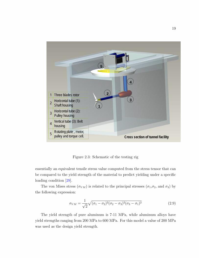
The testing rig basically consists of a three-bladed rotor attached to a main horizontal

shaft which drives the rotor, driven by a belt carried up through a vertical support

tube. The horizontal and vertical tubes that compose the support-structure are made

of aluminum tubing and are submerged in the water tunnel so that the motor and

instruments of the system are placed outside the water, on top of the cover of the water

tunnel, as shown Fig. 2.3. The scaled rotor has a diameter of approximately 15 cm,

and it will be placed at half of the water tunnel height (25 cm). Since the vertical

tube (main upright) should be positioned as far downstream of the rotor location as

possible, in order to minimize the disturbance in the near wake, the length of the

horizontal tubing (the sting) was expected to be between the 20 and 30 cm. This

corresponds to a number of complete wake revolutions downstream of the rotor that

could be characterized using PIV.

Several configurations of lengths, diameter and wall thicknesses for the tubing

support-structure were evaluated using ANSYS 11.0 in order to determine the mini-

mum possible sizes for the tubes. A structural static analysis was performed on the

loaded structure to estimate the maximum deflections. The intent was to have a rigid

structure so that aero and hydrodynamic validation could be carried out without

confusing the picture with coupled aero/hydro-elastic deformations. In addition, a

modal analysis was performed to obtain the natural frequencies in order to compare

with the external frequency imposed on the system by the rotor rotation. Details

of the FEM modelling, such as geometry and property materials, can be found in

Appendix B.

Once the minimum allowable sizes for the main tube components were determined,

the mechanical components of the model were chosen based on testing requirement

and availability in the market. The detailed drawings needed for fabrication, sum-

marized in the §2.4, were developed by a co-op student, Heshan Fernando [27].

2.3.1 Failure Criteria and Maximum Deflection

The maximum deflection accepted for the final design is restricted to 1.5 mm for

yawed conditions, and limited to a maximum value of 1 mm for the case of the rotor

plane facing the inflow orthogonally. The von Mises stresses available in ANSYS [28]

were used in the evaluation of failure for the tubing-material. The von Mises stress is

19

1

3

5

4

21 Three blades rotor

2 Horizontal tube (1):Shaft housing

3 Horizontal tube (2):Pulley housing

4 Vertical tube (3): Belthousing

5 Rotating plate , motor,pulley and torque cell. Cross section of tunnel facility

Figure 2.3: Schematic of the testing rig

essentially an equivalent tensile stress value computed from the stress tensor that can

be compared to the yield strength of the material to predict yielding under a specific

loading condition [29].

The von Mises stress (σVM) is related to the principal stresses (σ1,σ2, and σ3) by

the following expression:

σVM =1√2

√(σ1 − σ2)2(σ2 − σ3)2(σ3 − σ1)2 (2.9)

The yield strength of pure aluminum is 7-11 MPa, while aluminum alloys have

yield strengths ranging from 200 MPa to 600 MPa. For this model a value of 200 MPa

was used as the design yield strength.

20

2.3.2 Modal Analysis

A modal analysis was performed to determine the natural frequencies and mode

shapes of the support structure [30]. The purpose of this analysis was to determine

vibration characteristics of the testing rig structure in order to avoid coupling with the

spinning turbine blades while performing the experiments. In this particular model,

neither pres-stress nor damping was computed.

The basic equation solved in typical modal analysis without damping is the clas-

sical eigenvalue problem:

[K]θi = ω2i [M ]θi (2.10)

where [K] is the stiffness matrix of the structure, θi is the eigenvector (mode shape)

of mode i, [M ] is the mass matrix, and ωi is the eigenvalue (natural frequency) of

mode i. The modal analysis is solved using the consistent mass matrix. The natural

frequencies and mode shapes are equivalent to the solution of an eigenvalue problem.

Depending on the computation of damping and the resulting system matrices the

numerical effort to solve the eigenvalue problem may vary.

ANSYS provides a number of different eigenvalue solver options [31]. To solve the

eigenvalue problem the Block Lanczos Method was chosen. It is a fast and robust

algorithm and used for most applications as the default solver. It is recommended

when finding many modes, or when the model consists of mainly solid elements [28].

2.3.3 Summary of the FEM Results

Ten different configurations of tube length and wall thickness were defined and com-

puted in the analysis (Model1 to Model10). Table B.1 in Appendix B presents the

detailed dimension for the 10 configurations, where Tube1 is the horizontal tube that

houses the rotating shaft; Tube3 is the vertical tube that houses the vertical belt; and

Tube2 is the short tube that houses the pulley and connects Tube1 to Tube3 as shown

in Fig. 2.4.

Tube3 did not vary its length since the rotor must be placed at the half-height of

the tunnel depth, however wall thicknesses between 0.058 in and 0.12 in are considered

in the analysis. The same was true for tube2 of length 5 cm and thickness between

21

Y

Z

X

Rotor swept area

Inflow

HorizontalTube 1

VerticalTube 3

HorizontalTube 2

Figure 2.4: FEM tube model of the testing rig

0.058 and 0.12 in. Tube1 varied its length between 20 and 30 cm and wall thickness

between 0.058 and 0.12 in.

The results of the static analyses are provided in Appendix B, displayed in Ta-

ble B.2 to Table B.5. In the first model simulations, only four of the ten models

(Model7, Model8, Model9, and Model10) achieved maximum deflections within the

threshold value set up for the design. Based on this static analysis, the minimum

diameter for the horizontal tube that houses the spinning shaft (Tube1, the sting)

was 1/2 in with a minimum wall thickness of 0.065 in. The minimum diameter of the

vertical tube that houses the belt (Tube3) was found to be 3/4 in with a minimum

wall thickness of 0.12 in; and the minimum diameter of the shortest tube that houses

the pulley (tube2) is 3/4 in with a minimum wall thickness of 0.065 in.

The modal analysis was then computed for the selected models, and the first 10

modes extracted for the system composed of the three tubes and a mass representing

the rotor, as shown in Appendix B, Fig. B.1.

22

External forcing vibration frequency will be applied to the system due to the ro-

tating set of blades, during the testing. The rotor will spin in the range of 500 to

1500 RPM, which means frequencies in the range of 8.33 and 25 rev/s. To avoid vibra-

tion coupling, the natural frequencies obtained in this modal analysis were compared

to the frequencies associated with the operational conditions of the rotor. Details of

this analysis is presented in Appendix B, where in Table B.5 it is seen that natural

frequencies are higher than the external frequencies for Model5 to Model10. Since

at the time this modal analysis was done the final design was not yet finished, the

most robust and heavier structure (Model10) was chosen for determining the min-

imum diameters and wall thickness of the tubes that compose the structure. The

modal analysis results of Model10 allowed variation in the rig design without the risk

of increasing significantly the mass of the system and consequently decreasing the

characteristic vibration frequency of the structure.

The maximum length of Tube1, and recommended minimum thickness and diam-

eter for all the tubes that composed the rig structure are summarized in Table 2.3.

Dimension Tube1 Tube2 Tube3

Length [mm] 20 25 5Diameter [in] 0.75 0.75 0.12Thickness [in] 0.12 0.12 0.12

Table 2.3: Dimensions resulting from FEM analysis

2.4 Mechanical Design

This section presents a summarized description of the mechanical components that

compose the rig mechanical design. Detailed information is found in Fernando’s report

[27].

There were four main objectives that the testing rig design had to meet:

1. It must fit into a existing facility: the water tunnel of cross sectional area of 45

by 45 cm and height of 25 cm.

23

2. The driving system should provide speed control in order to measure power

output for different operational controlled conditions.

It is important to notice that frictional forces are not negligible for this model

size. The mechanical components of the rig, such as seals, bearings, belt, shaft,

etc, exert frictional forces and torque (Tfrictional) on the system, which could

be of the same order of magnitude as the hydrodynamic torque expected to be

measured from the rotor. Moreover, depending on the operational conditions it

is possible that the frictional torque is greater than the hydrodynamic torque

exerted by the fluid on the rotor. To better understating of this situation,

Fig. 2.5 shows a schematic of the externally applied torques identified in the rig

system.

The instrument load cell is attached to the case of the motor which runs the

system. The motor drives the belt which in turn drives the rotating shaft and

the rotor attached to it. Thydro is the hydrodynamic torque exerted by the flow-

stream on the system, Tfrictional is the torque due to static and dynamic frictional

forces of the mechanical components, and Treaction is the reaction torque at

the motor, read by the load cell, corresponding to the difference between of

hydrodynamic and frictional torque, Treaction = Thydro − Tfrictional.

Summarizing, a motor/generator (as opposed to simply a generator) is required

to overcome friction and to properly control the turbine when Tfrictional > Thydro.

Additionally, accurate control of the angular position of the rotor was required

for PIV post-processing phase/azimuthal correlation between blade and wake

positions.

3. The rig must have an area behind the spinning rotor where the disturbance

of the flow, due to the supports, is minimal. A distance of one to two rotor

diameters was imposed as a requirement for the horizontal tube that houses the

rotating shaft for this purpose.

4. The rig must allow testing in yawed flow conditions. For that, a yaw system is

required up to 45, ideally maintaining the rotor in the center of the tunnel to

avoid wall interference effects.

The main components of the final design are shown in Fig. 2.6. The top plates,

located on top of the cover of the water tunnel (as shown in Fig. 2.3) contain the

24

Torque Cell

Motor

Treaction

Belt

Shaft

Tfrictional

Thydro

Rotor

Figure 2.5: Schematic operation

instrument structure and the yaw system. The instrument structure consist of a

torque cell and the stepper motor that drives the system. The yaw system consists of

two plates attached to the hatch that can rotate and adjust position of the submersed

structure. The submersed structure is composed of several parts: the horizontal

rotating shaft and its housing tube, the rotor, the fairings that reduce the disturbance

of the flow, and the belt system and its corresponding housing tubes. The motor

drives the belt system which is connected to the rotating shaft which in turn drives

and controls the speed of the rotor.

2.4.1 Instrument Structure

Figure 2.7 presents a schematic of the instrument structure.

25

Instrument Structure

Yaw System

FairingsSubmerged Structure

Belt Drive

Figure 2.6: Key components of the rig

Plates and posts compose the structure that houses the motor and torque cell.

The torque cell is attached to one plate; the motor is attached to the torque cell and a

flexible coupler attaches the output shaft of the motor to the pulley shafts that drives

the belt system. Bearings are used to minimize the friction, and a clamp attaches

the vertical tube support of the submerged structure to the instrument structure.

Since the measurements must be very precise, alignment is critical for this design.

The plates and posts are accurately machined to meet these requirements. Holes are

made on the plate that accurately mate with bosses machined on the posts. Further

details of the motor and instruments are provided in Chapter 5.

2.4.2 Belt System

In order to minimize the friction of the rotating components, a belt was chosen to drive

the submerged rotating shaft (which runs the rotor). This option has less friction than

26

Torque-cell

Stepper Motor

Housing

Coupler

Clamp

Figure 2.7: Components of the instrument structure

using a rotating gear system. The spinning rotor will reach high rotational speed, up

to 1500 RPM, which can lead to additional vibration in the system. To check this

design choice, a rig for belt testing was fabricated before carrying out the final design

of the testing rig.

To asses two different belt options, and to check the level of vibration of the system

in the range of rotational speeds considered for the final experiment, belt testing was

performed in this early design stage. The belts were ordered from SDP/SI products;

Table 2.4 present the characteristic of the two belt tested [32]. Pulleys were also

ordered from SDP/SI, each type corresponding to the belt model.

The rig designed for the belt testing had a support structure made of two ply-

wood platforms and two aluminum posts, as shown in Figure 2.8. The mechanical

components for the testing were the motor, the belt, two pulleys (one attached to

the output shaft of the motor and the other located in the lower platform), and a

bearing system that houses a free-spinning shaft located in the lower platform. Is was

27

Figure 2.8: Rig for belt testing

possible to adjust the location of the motor in the vertical plane by fastening four

screws, which provided the tension required for the belt to work properly. The test

was run for rotational speeds in the range of 60 RPM to 1500 RPM.

As a result of this testing, vibrations were noticed only at very low speeds, below

500 RPM. The belt type MXL ran smother than the belt type GT3; this may be

because belt type GT3 was found to be stiffer than belt type MXL. In addition, the

pulley corresponding to belt GT3 used a set screw to attach to the output shaft of

the motor, what caused slight damage to the shaft, whereas pulley of belt MXL had

a clamp. In conclusion, belt MXL was chosen for the final testing rig.

28

Model number Material body Materialcord

Pitchlength[in]

No of.grooves

MXL A6G16-350025 polyurethane polyester 28 350GT3 A6R53M250060 nylon covered fiber-

glass reinforcedpolyester 29.5 250

Table 2.4: Characteristics of the candidate belts

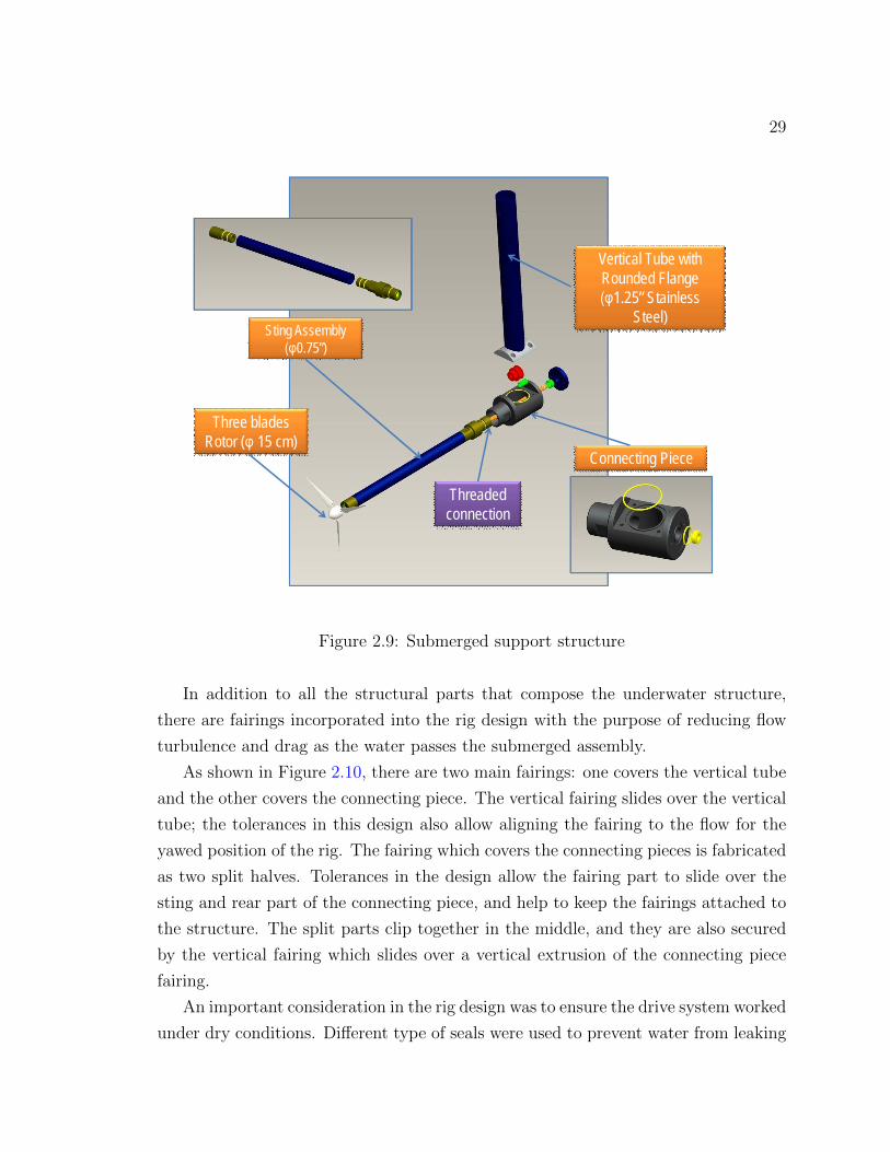
2.4.3 Submersed Structure

The submerged structure is composed of a rotor, a sting, a connecting part, a vertical

tube, and a set of fairings, as shown Figure 2.9. The aim of this particular design

was to make the components of this structure as small as possible to avoid blockage

effects and flow disturbances. In addition, the sting had to be as long as possible in

order to provide an undisturbed area behind the rotor for the PIV images to be taken.

The sting is the part that houses the rotating shaft which is attached to the rotor.

This assembly part is made of aluminum tube of 0.75 in external diameter, and has

two press-fitted pieces at each end, one of them containing threads that attach this

structure to the connecting piece.

The connecting piece connects the sting assembly and the vertical tube which

suspends the submerged structure from the rig-plates. This connecting piece is made

of aluminum and has an overall outside diameter of 2 in. It was not possible to make

this piece smaller since it has to provide sufficient room to locate the pulley that

drives the shaft inside this connecting piece. For the sting assembly to be attached

and aligned to this connecting piece, a bore and threads were designed in the front

part.

There is a vertical tube that houses the belt which compose the rig drive system.

The vertical tube, made of stainless steal of 1.25 in diameter, connects the submerged

structure to the upper instrument structure, and keeps the sting assembly at the

center of the vertical tunnel cross-section. A flange is welded at the bottom of the

tube to secure it by screws to the connecting piece.

The blades and hub that composed the three-blade rotor design are fabricated in

the SSDLs lab, using the FDM machine as described in section next.

29

Connecting Piece

Vertical Tube withRounded Flange

1.25” StainlessSteel)

Three bladesRotor ( 15 cm)

Sting Assembly0.75”)

Threadedconnection

Figure 2.9: Submerged support structure

In addition to all the structural parts that compose the underwater structure,

there are fairings incorporated into the rig design with the purpose of reducing flow

turbulence and drag as the water passes the submerged assembly.

As shown in Figure 2.10, there are two main fairings: one covers the vertical tube

and the other covers the connecting piece. The vertical fairing slides over the vertical

tube; the tolerances in this design also allow aligning the fairing to the flow for the

yawed position of the rig. The fairing which covers the connecting pieces is fabricated

as two split halves. Tolerances in the design allow the fairing part to slide over the

sting and rear part of the connecting piece, and help to keep the fairings attached to

the structure. The split parts clip together in the middle, and they are also secured

by the vertical fairing which slides over a vertical extrusion of the connecting piece

fairing.

An important consideration in the rig design was to ensure the drive system worked

under dry conditions. Different type of seals were used to prevent water from leaking

30

Fairings

Figure 2.10: Model of fairings covering the submerged structure

inside the underwater structure. O-rings and grooves were placed between two mating

surfaces or press-fitted pieces, and lip seals were used to prevent water entering around

the rotating surfaces like the rotating shaft in the sting.

Finally, notice that three axial bearings were used in this design to align and

minimize the friction for the rotating shaft. There are two bearings on the sting, and

a third bearing placed in the rear part of the connecting piece

2.4.4 The Rotor

A 3D material printer available in the Sustainable System Development Lab (SSDL)

using FDM techniques was utilized for building the rotor blades (and a number of

fairings and other parts of the rig). This technology allows construction in-house

of several parts in a short period of time. Then, different blade profiles and sizes

can be tried in the ongoing and future experiments. A wide range of thermoplas-

tics with different mechanical properties can be used as printing material; ABS and

Polycarbonate (PC) thermoplastics were available for building the parts.

Depending on the material employed, it is possible to accurately manufacture

small parts by extruding material into layers as thin as 0.005 in thickness (T10 tip).

31

For the first set of blades the material used was PC, and the T12 tip was used which

creates a layer 0.007 in thick. Build time and part finish are proportional to the tip

size used.

The 3D printer, a Fortus 400mc, works with the Insight software. This application,

installed on the user’s work station, allows setting up the properties of the parts to

be printed, such as surface smoothness, layer path, filling spaces, void volume, etc.

Figure 2.11: Rotor assembly

Figure 2.11 shows the blades and hub parts that were made separately and then

assembled together. The upstream end of the rotating shaft has a boss to prevent

the hub part from touching the sting assembly (Fig. 2.9) and to align the hub part

with the submerged structure. It also has threads allowing the hub-part to be secured

against the shaft.

The three blades have identical profile, are about 70 mm long, 25 mm wide at the

root, and 7 mm wide at the tip of the blade. The root part has a circular plate plane

orthogonal to the span-wise axis, which is used to keep the blade clamped between

the two-half hub parts. The hub part is composed of two cylindrical parts meant to

clamp the blades and to provide pitch adjustment. A hexagonal nut is used to secure

the hub against the shaft boss. The nose cone is attached to the hub part covering

the hex-nut.

32

The initial set of blades built correspond to a NACA63(2)-4XX airfoil profile, with

21 % thickness, and a twist angle of 15. This relatively large thickness airfoil was

used to ensure blade rigidity.

2.4.5 Yaw System

The yaw system works due to the motion of two concentric planes of rotation: the

plane of the instrument structure plate, and the circular rotating plate. The former

has an axis of rotation about the vertical support tube, and the latter about the water

tunnel cover cutout hole.

As shown in Fig. 2.6, the vertical tube which holds the submerged assembly is

clamped to the instrument structure. This instrument structure is placed above the

circular rotating plate, and secured to the plate by screws. The circular rotating plate

is seated on a hole made in the cover of the water tunnel, and is kept attached to the

hatch by six clamping pieces and 24 screws.

Figure 2.12 demonstrates the yaw motion for the rig. The starting point in shown

in the scheme number 1 of the reference figure. First the circular plate rotates,

generating rotation of the the instrument structure, the vertical tube clamped to it,

and all the submerged structure attached, as shown in part 2 of the figure. Then,

the angle of the sting can be adjusted by rotating the instrument structures plate, as

shows part 3 of the figure. In such a way, it is possible to get different yaw angles

but keep the rotor at the center of the cross-section of the water tunnel.

Marks for the degree movements are included for both the rotating circular plate

as well as the base plate of the instrument structure. The maximum yaw angle

obtainable with the original rig design, with a sting of 13.25 in length, is about 23.

It is possible to reach 45if the sting assembly is replaced for a shorter one of 7.42 in

length. In the end, two different sting assemblies were built allowing different yaw

capabilities for the final testing rig. At present, the yaw system is actuated manually

and fixed during testing. In the future, this system could be automated to enable

dynamic yaw event testing.

33

Figure 2.12: Yaw system operation

2.5 Instrumentation

The general layout of the complete rig and PIV system is depicted in Fig. 2.13.4 There

are two acrylic hatches that cover the water tunnel at the upper surface allowing the

section to operate closed instead of having a free surface. As described in §2.4.3, the

whole instrument and drive system is kept outside the water tunnel. The rotor is

located at the center of the section to minimize wall effect over the measurements.

The DPIV system is comprised of a camera and a laser sheet, and will be used

to illuminate a horizontal plane and capture the particle images in the near wake.

The area of interest is located behind the rotor up to a few diameters downstream.

4The terms Digital Particle Image Velocimetry (DPIV) and PIV as used in this thesis bothstrictly refer to a DPIV system, as the images are digitally acquired and processed.

34

Laser

system

Front View Side View

Camera Camera

Laser

sheet

Vector velocity field

Area of interest

Figure 2.13: PIV system layout

The X-Y plane is parallel to the bottom and roof of the water tunnel, the flow is

in the X axis direction, from left to right, and the Z-axis points upward. The laser

sheet illumination is the X-Y plane, and the camera is located perpendicular to the

illumination plane looking upwards. This general layout is meant to avoid, or at least

minimize, shadows in the wake. When illuminating the same plane from the bottom,

the vertical tube, that contains the shaft, will probably generate shadows in the area

of study. On the other hand, this vertical tube will be positioned as far aft the rotor

as is possible in order to minimize the disturbance in the near wake.

The interactions among the components of the integrated electric system that

control the experiment are shown in Fig. 2.14. The main components of the integrated

system are:

• The rotor itself, imparting torque on the shaft. This torque is transmitted to

the drive system by the rotating shaft and belt system.

• The drive system, which runs the rotor, comprised of a stepper motor and the

E-AC Driver.

35

• The Data Acquisition System (DAQ) system is composed of the instrument to

measure the torque of the motor, the loadcell, and by the control and data ac-

quisition system, the NI CompactRio hardware. The CompactRio technology

is a real time acquisition system which allows control of the drive system, trig-

gers the PIV system to start, and stores all the information acquired. LabView,

installed on a user computer, provides a user interface for the DAQ system.

Through this software it is possible to display the information being acquired

and command the motor velocity and direction, and to start and stop the sys-

tem.

• The PIV system is an independent piece of hardware with its own controller

system and storage capacity. It cannot be commanded by the CompactRio

directly to take a picture, but it can be triggered to start operation. It is

composed of a laser, a digital camera, and operating software, LaVision. The

laser system was the component that was broken during most of the thesis

period and precluded operation of the PIV for the trial runs of the rig discussed

in Chapter 5.

2.5.1 The Drive System

In order to meet the objectives of the experiment, it was important to have control

over the operational conditions of the turbine. It was also desirable to be able to

control the rotational position of the rotor, and minimize the number of components

and electric equipment working within the system.

Stepper motors allow precise positioning and speed control without the use of

encoder or feedback sensors. The stepper motor and the drive selected allows the

shaft to move only a set number of degrees when each pulse is delivered by the drive.

The stepper motor HV233 and the E-AC 120 V AC Microstepping Drive from Parker

were chosen as the drive system, as shown in Fig. 2.15. The E-AC Microstepping

Drive can be plugged directly into the standard mains supply (ranging between 95 to

132 V AC), and can be integrated to the Compact Rio technology control.

BEM simulation runs for comparison to the experimental results were typically

done setting an angular accuracy of 5 . Consequently, providing rotor control with

the best angular accuracy is desirable for measurement and comparison. In others

words, given the accuracy required on angular position, a restriction on the minimum

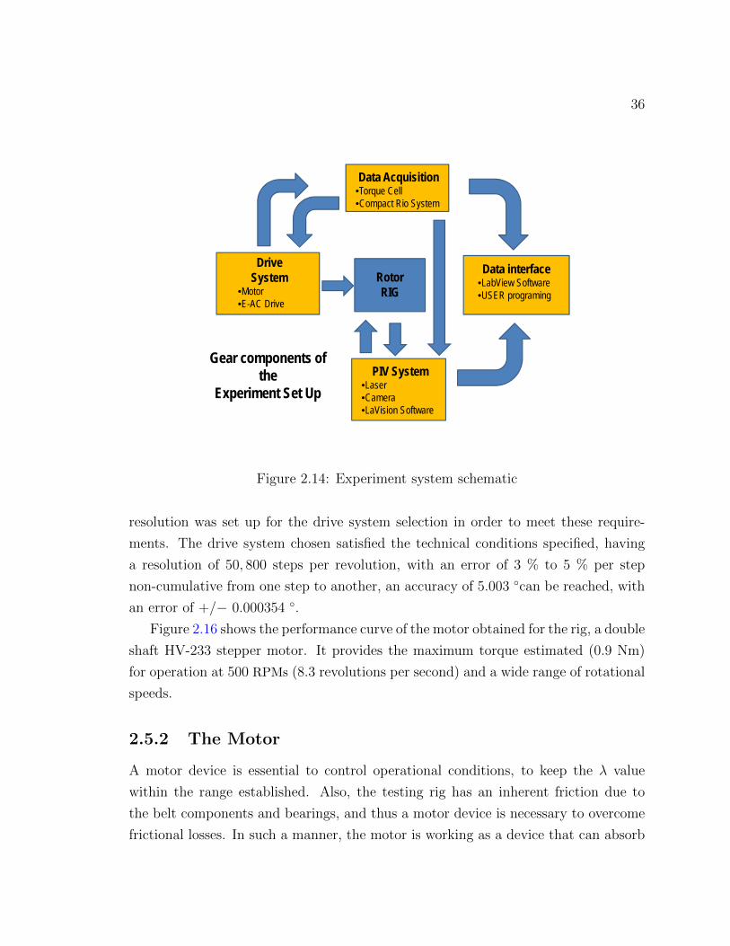
36

RotorRIG

DriveSystem

•Motor•E-AC Drive

Data Acquisition•Torque Cell•Compact Rio System

PIV System•Laser•Camera•LaVision Software

Data interface•LabView Software•USER programing

Gear components ofthe

Experiment Set Up

Figure 2.14: Experiment system schematic

resolution was set up for the drive system selection in order to meet these require-

ments. The drive system chosen satisfied the technical conditions specified, having

a resolution of 50, 800 steps per revolution, with an error of 3 % to 5 % per step

non-cumulative from one step to another, an accuracy of 5.003 can be reached, with

an error of +/− 0.000354 .

Figure 2.16 shows the performance curve of the motor obtained for the rig, a double

shaft HV-233 stepper motor. It provides the maximum torque estimated (0.9 Nm)

for operation at 500 RPMs (8.3 revolutions per second) and a wide range of rotational

speeds.

2.5.2 The Motor

A motor device is essential to control operational conditions, to keep the λ value

within the range established. Also, the testing rig has an inherent friction due to

the belt components and bearings, and thus a motor device is necessary to overcome

frictional losses. In such a manner, the motor is working as a device that can absorb

37

Figure 2.15: Drive system

and provide power, and that allows the net torque of the rotor minus all the losses in

the drivetrain to be determined.

In retrospect, while the stepper motor is advantageous in providing speed and

position control without feedback, two issues were found in practise. In order to

attain the required torques, the coils were connected in series, but this caused the

motor to overheat when run longer than 10-20 minutes. In addition, the first motor

obtained had some flaw that caused stalling even in no-load conditions. The situation

was hard to address, even after multiple attempts at ensuring alignment of matings

surfaces, etc. Again, this greatly delayed the experiments, and eventually lead to

replacement of the first motor. Perhaps a better approach for future rigs would be

a servomotor with encoder feedback positions, although high-accuracy encoders for

fine knowledge and control of azimuthal position could be challenging to obtain.

2.5.3 Torque cell

Notice that for small scale models, accurate force measurement is extremely difficult

to achieve due to the level of noise in the signals, thus only torque measurement was

feasibly for this study. Thrust force measurement was considered, but was considered

impractical given the other constraints of the system and the primary requirement

for excellent torque and azimuthal position control.

The Novatech F326-Z 1 Nm loadcell was chosen to measure the reaction torque of

the motor. This type of loadcell fits between a motor and its mounting structure act-

38

HV233

Figure 2.16: Performance curve Parker Motor HV233

ing as a coupling. Novatech proposed two options for the F326-Z mounting, Fig. 2.17,

for this rig. The configurations suggested are meant to support the motor weight and

remove any extraneous forces and bending moments, if the mounting structure and

bearings for shaft supports are properly aligned. At one side of the loadcell, four

screws are used to fasten the motor to the torque cell structure so that the motor’s

torque is transmitted to the F326. This flanged mounted motor torque transducer

has a hole through the axial centre of the structure, which allows the motor shaft

to pass through it. On the other side of the loadcell another four screws are used

to fasten the loadcell to the instrument rig structure. The rig instrument structure

follows the first scheme of Fig. 2.17 (single shaft mounting), but utilizing a double

shaft motor as described in §2.4. The reaction torque is therefore measured between

the case and mounting (earth) structure.

With respect to the torque range measurement and its resolution, the loadcell has

the capability to measure torques ranging -1 Nm to +1 Nm, and read values as small

as the minimum expected torque for the experiment, which is 0.01 Nm, providing the

DAQ electronics components can handle the small signal of 60 µV.

The F326-Z loadcell has a nominal output of 0.6 mV/V, which basically deter-

mined the selection of DAQ CompactRio module in charge of torque measurement.

Given the minimum torque value to be read (i.e 0.01 Nm), and a 10 volt excitation

voltage for the torque cell, this specific DAQ module must be capable of reading a

small signal of 60 µV.

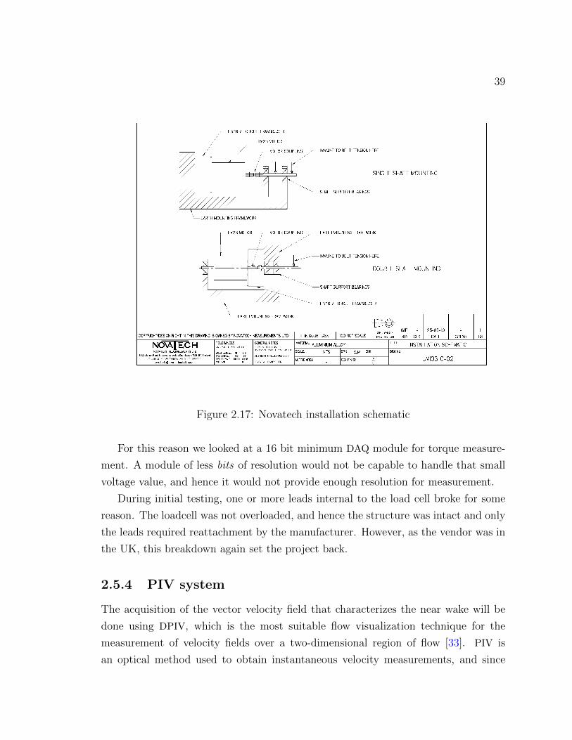
39

Figure 2.17: Novatech installation schematic

For this reason we looked at a 16 bit minimum DAQ module for torque measure-

ment. A module of less bits of resolution would not be capable to handle that small

voltage value, and hence it would not provide enough resolution for measurement.

During initial testing, one or more leads internal to the load cell broke for some

reason. The loadcell was not overloaded, and hence the structure was intact and only

the leads required reattachment by the manufacturer. However, as the vendor was in

the UK, this breakdown again set the project back.

2.5.4 PIV system

The acquisition of the vector velocity field that characterizes the near wake will be

done using DPIV, which is the most suitable flow visualization technique for the

measurement of velocity fields over a two-dimensional region of flow [33]. PIV is

an optical method used to obtain instantaneous velocity measurements, and since

40

optical measurements avoid the need for Pitot tubes, hotwires or other physical flow

measurement probes which cause disturbance of the flow field, this method has the

advantage of being a non intrusive measurement technique.

The fluid is seeded with tracer particles which are supposed to cause negligible

distortion of the fluid flow. These particles have to be carefully chosen depending

of the type of fluid and motion to follow the flow dynamics. For this particular

experiment, Mearlin Supersparkle particles were available with mean diameters in

the range of 5 to 7 µm and silver in colour. The specific gravity of these particles is

larger than specific gravity of water, thus they are deposited on the bottom of the

channel when the water tunnel is off. However, it is possible to infer from others’

experiments carried out in the same tunnel facility and having the same type of

particles [34], that the flow speed considered for this particular experiment is high

enough to keep the particles following the motion of the flow field.

Lens(camera)

Sensor plane(in camera)t + t

t

Seededflow

OpticsDouble pulselaser

Laser sheet

Figure 2.18: General schematics of PIV system

Notice that it is the motion of these tracer particles that makes visible the fluid

motion. By recording the position of them at different instances of time, is possible

41

to determine the displacement of the particles in this time interval, and to calculate

its velocity, and eventually build up the flow velocity field.

To capture the image of displacement of the tracers, typically DPIV uses digital

cameras with frame rates on the order of 15 - 30 Frames per Second (FPS). To

freeze the movement of the particles at specific time, a laser pulse of light is used

to illuminate the plane of motion. In this way, the sensor of the digital camera is

able to capture the movement of the small particles. Finally, the images taken are

processed in a computer to reconstruct the whole velocity field. The schematics of

this technique is presented in Fig. 2.18.

There are some factors relevant the DPIV measurement technique, such as timing

of the camera shooting, laser pulse, and the size of the interrogation cell. For instance,

to get accurate measurements it is crucial to synchronize the camera shutters and laser

pulse. Also, the size of the interrogation cell (typically size 6x6 pixels) will depend

on the conditions of the flow to be measured. Ideally there are between 3 and 15

particles per area of interrogation. Thus depending on the seeding density, the size of

the seeding particle, and the velocity of the flow field, there is a cell size that satisfies

that ideal condition and this must be set up for each particular experiment event

(a trial and error process). More detailed information about PIV theory is given in

Appendix C.

For this particular experiment, in an attempt to reconstitute the 3D velocity fields,

PIV images are intended to be taken for a set of different azimuthal planes, each one

representing a cross-section of the wake [2]. It is important to notice that PIV images

are basically 2D, in this case taken at the plane parallel to the inflow velocity. The set

of azimuthal planes are obtained by triggering the camera to take single 2D pictures

at different timings relative to the rotor, in such a way that each picture will capture

the instantaneous flow velocity corresponding to the vertical position of the blades

set at different angles. This will also allow for azimuthally averaged flow quantities

to be computed.

The available PIV equipment in the Fluid Lab consisted of a high speed digital

camera, a Quantronix Nd:YLF laser, and a PC with hardware for DPIV image data

acquisition. For the experiment, the task is to the synchronize the PIV recording

equipment with a defined angular position of the rotor, in order to obtain flow pho-

tographs at any predetermined position of the blades. This was the primary reason

for selection of a stepper motor, and a control system able to trigger the PIV image

42

recording.

The Darwin-Duo laser series, a 25 mJ Nd:YLF dual diode-pumped type, can be

externally triggered via TTL Inputs in such way that the PIV hardware starts the

laser operation. At each input signal, the laser provide two laser pulses, having a

pulse width of 120 ns and a frequency ranging between 0.1 to 10 kHz. This allows

control of the time intervals between each of them with a resolution of 25 ns, and a

timing jitter below 2 ns.

The laser optics provides a planar light sheet to illuminate the particles in the

region of interest. The digital camera is a HighSpeedStar HSS − 5 CMOS sensor

with frames rates up to 250 kHz, a maximum resolution of 1024x1024 pixel for a

frame rate of 3 kHz and below, and a minimum interframe time of 2 µs.

The images taken are sent to the software LaVision DaVis 7.2 for data processing.

Within the software the recorded images are evaluated by cross-correlating pairs of

frame, each containing single exposure of the group of markers (This PIV technique

is detailed in Appendix C).

Basically, the required settings for recording images are previously set up in the

DPIV PC Hardware, such as pixel size, frequency of image capture, etc. There is a

time delay between the starting time of the laser and the moment the camera capture

the first picture. Thus, there is also a set time delay before the camera starts in order

to synchronize with the laser pulses. Finally, the external trigger starts the DPIV

hardware, which triggers the laser and the image acquisition.

Ideally the whole system can be programed to capture an image every turn of the

rotor at specific position. However, because of the high rotation speed of the scale

model rotor, it is probable that the camera must be set up to capture the images

every two or three turns. The final frequency and operation of this integrated system

must be adjusted in a trial an error exercise once the PIV system is again operational.

2.5.5 DAQ Rio System

The NI CompactRio package was selected as a combined control and DAQ system.

This technology is portable, it communicates over the network, contains a real-time

processor, a reconfigurable field-programmable gate array (FPGA), and a variety of

analog and digital input/output modules to cover the requirements for the experi-

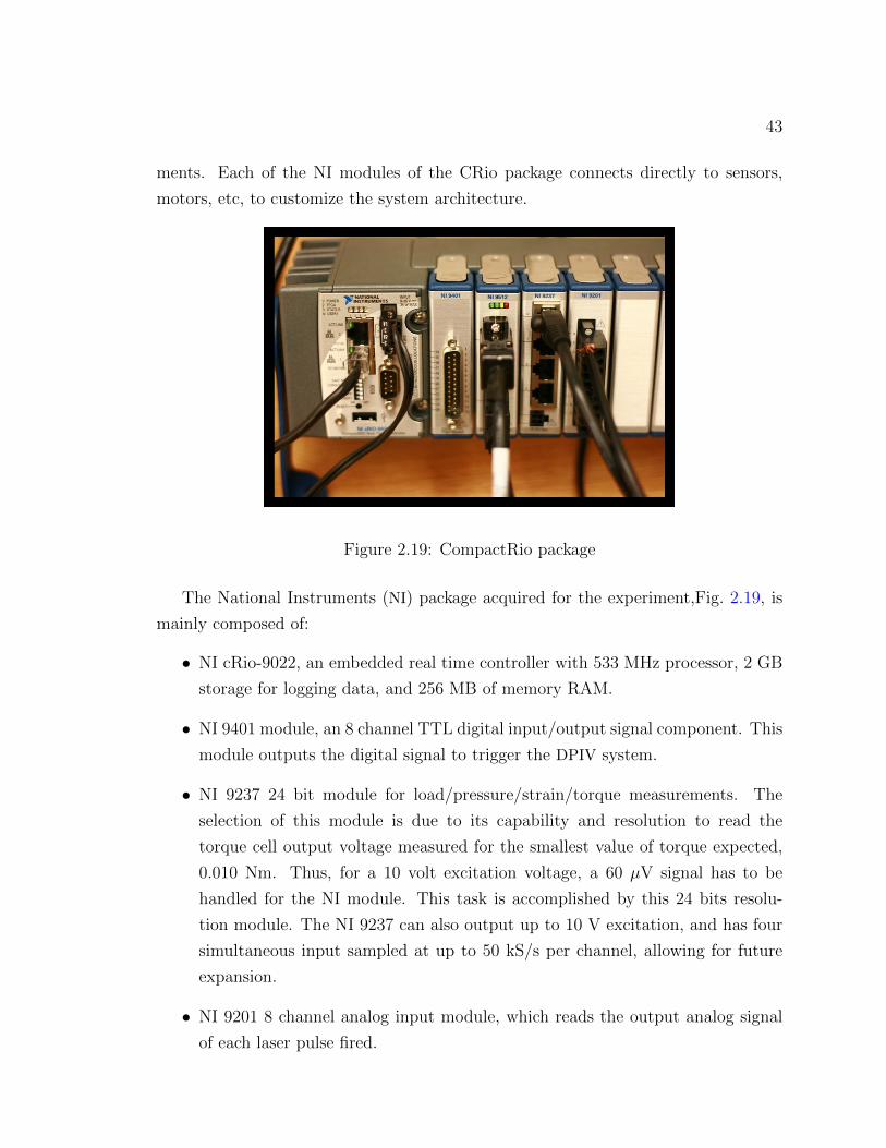
43

ments. Each of the NI modules of the CRio package connects directly to sensors,

motors, etc, to customize the system architecture.

Figure 2.19: CompactRio package

The National Instruments (NI) package acquired for the experiment,Fig. 2.19, is

mainly composed of:

• NI cRio-9022, an embedded real time controller with 533 MHz processor, 2 GB

storage for logging data, and 256 MB of memory RAM.

• NI 9401 module, an 8 channel TTL digital input/output signal component. This

module outputs the digital signal to trigger the DPIV system.

• NI 9237 24 bit module for load/pressure/strain/torque measurements. The

selection of this module is due to its capability and resolution to read the

torque cell output voltage measured for the smallest value of torque expected,

0.010 Nm. Thus, for a 10 volt excitation voltage, a 60 µV signal has to be

handled for the NI module. This task is accomplished by this 24 bits resolu-

tion module. The NI 9237 can also output up to 10 V excitation, and has four

simultaneous input sampled at up to 50 kS/s per channel, allowing for future

expansion.

• NI 9201 8 channel analog input module, which reads the output analog signal

of each laser pulse fired.

44

• NI 9512 stepper drive interface module. This module is probably the most

complex of the package. It has its own power supply, and acts as the controller

of the drive system. This module makes if possible to control rotation speed and

direction of the motor when running, without the need to stop the movement.

It also allows moving the rotor in discrete steps.

• NI LabView software, a graphical tool developed by NI can be installed in the

user’s laptop for designing, prototyping, and deploying embedded applications.

The control software for the entire system was implemented in LabView. Fig-

ure 2.20 depicts a screen shot of the developed LabView interface software. The

figure displays the basic functions programmed such as velocity control, data

recording onset, PIV triggering option, data position display, torque measured

display, etc.

Figure 2.20: LabView interface

45

Chapter 3

Computational Fluid Dynamic

Simulations

This CFD study focuses on providing information that can be used to properly correct

the data acquired in the experiment performed in the water tunnel, which is known

to be affected by blockage due to the walls of the tunnel facility, as described next

in Chapter 4. Since the experimental data obtained must be corrected to unbounded

flow conditions (see §4.1), a key point presented in this CFD chapter is the unbounded

model domain validation. The study also included ReD dependency analysis to verify

the validity of the simulations results for a range flow conditions.

This chapter has two main sections which describe the computational modelling

approach used to represent the fluid phenomena of kinetic turbines operating in water

tunnel and free stream conditions. The first section presents the conceptualization

of the turbine and physical domain in such a way that can be translated into a

simple computational model. In this context, the rotor has been conceptualized as a

continuous plane that extracts energy from the flow. Suitable boundary conditions

have been set up to the model in order to represent both scenarios, the water tunnel

and open flow conditions. The second section of this chapter presents the details of

the computational tools used for these purposes. Note that this second section is an

overview description of the mathematical equations employed in the ANSYS CFX

tool, but is not an exhaustive text on CFD.

46

3.1 Modelling Approach

3.1.1 Porous disk

Several approaches have been used to model the aerodynamics of horizontal axis

wind turbines [3]. Regarding the near wake, the porous or actuator disk technique

has been widely utilized in numerical models, as well in experimental testing applied

to horizontal tidal stream turbines [12, 35]. This porous disk model has the advantage

of requiring a reduced mesh density compared to other available numerical models for

CFD simulations [3, 35]. Thus, it is computationally less expensive, and it is utilized

to simulate the blockage effects in this study.

Because this method conceptualizes the rotor as a plane which extracts energy

from the flow, a drawback of this model is that the blades of the turbine are not

directly simulated. However, considering the objectives of these CFD simulations,

this approach is adequate to meet the study purposes.

The total pressure drop that the actuator disk area exerts on the fluid is repre-

sented by a unidirectional momentum loss, or thrust force per volume unit, χ applied

at the disk volume. For the CFD simulations, this momentum loss is rewritten in

terms of the thrust coefficient (CT ), the upstream axial inlet velocity (U0), the water

density (ρ), and the thickness of the disk (t), as presented in Eq. (3.3). Equation (3.3)

is obtained by equating the thrust force from Eq. (3.1) and Eq. (3.2), as follows:

T =1

2ρAU2

0CT (3.1)

χAt = T (3.2)

χ =12ρU2

0CT

t(3.3)

3.1.2 Domain

The simulations were run over two different computational domains. The first domain

accounted for the unbounded conditions where no wall prevents the streamlines from

expanding freely. The second computational domain models the water tunnel, which

allows for comparison between experimental and full scale conditions.

Defining D (15 cm) as the diameter of the scaled rotor being tested, the rectan-

gular water tunnel computational domain has a cross-sectional area of 3Dx3D and

47

a length of 15D, and the disc is placed 5D downstream of the inlet centred in the

tunnel section, corresponding to the experimental setup. The unbounded rectangular

computational domain is defined with a section of 6Dx6D, 25D long, and the disk

located 5D downstream from the inlet. For both cases, a structured mesh was gener-

ated using ICEM, applying O-grid and blocking topology features that facilitate the

manipulation of the grid for a 3D model.

As detailed in the boundary conditions section next, symmetry is applied to the

original model described, which allows the simulations to be run over a quarter-

domain as shows scheme in Fig. 3.1.

Figure 3.1: Quarter domain water tunnel model (ANSYS CFX)

By computing simulation results for four different rotor sizes, the effects of block-

age ratio were explored, where blockage ratio is defined as the ratio of rotor swept

area to tunnel section area (A/Atunnel). The thickness of the disc was fixed at 0.5%

of the rotor diameter (0.005D) in all cases.

48

3.1.3 Boundary Conditions

A uniform axial velocity of 2 m/s was set up at the inlet of the domains. This

boundary condition is physically driven by the pump in the water tunnel, and also

represents the operational expected flow velocity in the open water. At the outlet, an

average static pressure was defined, with relative pressure equal to zero. Specifying

an average static pressure over the whole outlet allows the pressure variable to vary

locally over the outlet boundary such that the average pressure is constrained to a

specific value. Physically, this may be the situation of the experiment with a higher

velocity at the centre of the section and lower near the wall region. Additionally, this

boundary condition configuration is listed as the most numerically robust option in

Ansys CFX [36].

At the actuator disk a unidirectional momentum loss χ (referring to Eq. (3.3))

was applied to account for the pressure drop for each CT value computed. Since

a quarter domain was used, two symmetry planes were applied, in the vertical and

horizontal planes respectively. These boundary conditions were also active for the

area of the disc in contact with these symmetry planes. For the unbounded domain,

an opening boundary condition, allowing fluid to cross the boundary surface but

keeping a constant pressure value at the boundary, was applied to the walls. For the

water tunnel domain, the base case considers a free-slip wall condition.

Even though free-slip conditions at the walls were previously defined as a bound-

ary condition in order to compare the CFD results to the analytical expressions for

blockage discussed in §3.3, additional simulations were run to investigate the effects

of the boundary layer growth within the tunnel. A minimum number of 10 nodes

within the boundary layer is suggested by the ANSYS CFX Guidelines [37] for the

near-wall turbulence model to work properly. For a turbulent boundary layer on a

flat plate in similar flow and fluid conditions, the viscous sublayer thickness should

be less than 1 mm [38]. Thus, to include the effects of viscous losses at the boundary,

a mesh having 10 nodes within this first 1 mm layer was generated from the wall to

properly computed the boundary layer [36]. The dimensionless wall distance is known

as y+ = u∗yν

where the friction velocity is u∗ =√

τwρ

and tw is the wall shear stress.

In the simulations run, y+ was approximately 10.

The water tunnel used for testing has a very low turbulence level (approximately

1%) which was used in the simulation inputs. Both laminar and turbulent flows were

computed. The Reynolds Average Navier-Stokes (RANS) equations were solved for

49

steady and incompressible flow, using a finite-volume method, and the K−Ω equation

was used to model the turbulence, as described next in §3.2.1.

3.2 Computational Model

The academic version 12.0 of the commercial package ANSYS CFX was used for the

three-dimensional CFD simulations, and the structured mesh over the domain was

generated using ANSYS ICEM.

The Navier-Stokes equations for mass-flow and momentum can be discretized and

solved numerically using diverse solution methods. The CFX package corresponds

to a particular CFD code based on a finite volume technique [39] in which the fluid

region of interest is split into smaller sub-regions, so called control volumes. This

subdivision allows an iterative solution of the set of partial differential equations for

each small sub-region. Finally, an approximate solution of the variables of study is

obtained, point by point, over the entire flow field domain.

3.2.1 Governing Equations

The basic equations of fluid mechanics, for describing the fluid motion, are the Navier-

Stokes equations, Eq. (3.4) and Eq. (3.5), where ρ is the fluid density, u the vector

velocity, p the pressure, τ the stress tensor, and SM the additional scalar term rep-

resenting a momentum source (refer to section next 3.2.2). Equation (3.4) is known

as the continuity equations, and Eq. (3.5) is called the momentum equation. These

general N-S equations are valid for both turbulent and non-turbulent flows, steady

and non steady conditions. The energy equations were not required, as the change in

fluid properties with temperature are negligible in the cases under investigation.

− ∂ρ

∂t+∇(ρu) = 0 (3.4)

− ∂(ρu)

∂t+∇(ρu⊗ u) = −∇p+∇ · τ + SM (3.5)

The fluid conditions that characterize the experiments performed in the water

tunnel makes it necessary to incorporate turbulence in the CFD model. Turbulence

occurs when the inertia forces in the fluid become important relative to viscous forces

50

(i.e. higher Reynolds numbers). In CFD modelling turbulent flows can be thought of

as an average characteristic, with an additional random fluctuation superimposed in

time and space. Thus, the turbulent flow can be statistically modelled for example as

an instantaneous velocity expressed as the sum of the mean velocity and a fluctuating

component Eq. (3.6), where the mean velocity is estimated as expressed in Eq. (3.7).

u = u+ u′ (3.6)

u =1

∆t

∫ 1+∆t

t

udt (3.7)

This statistical technique is applied to the Navier-Stokes equations producing the

RANS equations. For this particular model the governing equation for the turbulent

and incompressible flow are the RANS equations. The averaged quantities are sub-

stituted into the general transport equations and rearranged, resulting in Eqs. (3.8)

and (3.9):

−∂ρ∂t

+∇(ρu) = 0 (3.8)

−∂(ρu)

∂t+∇(ρu⊗ u) = −∇p+∇ · (τ − ρu⊗ ·u) + SM (3.9)

where the terms ρu⊗ ·u have the same structure as the viscous stress tensor and

are called Reynolds Stresses, however these terms arises from a non-linear convective

term contribution of the fluctuating velocities to the change of the averages ones. The

Reynold stress tensor incorporates additional unknown variables to be solved in the

CFD model, generating a closure problem.

Since this study considers stationary flow conditions, the varying-time terms in

Eq. (3.8) and Eq. (3.9) become zero. Notice that ANSYS CFX is an iterative solver

which approaches the solution of the set of partial differential equations over a set

of iterations. The solver therefore uses a timestep for iteration process, used only to

under-relax the governing equations.

In order to achieve closure for equation Eq. (3.9), turbulence models are intro-

duced to compute the Reynolds stresses and fluxes. Depending on the assumptions

of these models, there are two main types available in CFX: eddy viscosity models

and Reynolds stress models [36]. For this study, to achieve closure, the K −Ω model

51

was used, which is part of the family of eddy viscosity two-equation turbulent models.

This model has become a widely used turbulence model [40], which can predict effects

for both free shear flows (which is the case of the wake behind the rotor in this study)

and wall-bounded boundary layer flows with reasonable accuracy provided a good

detailed mesh is used, as indicated in §3.1.3 [36]. Considering the simulations com-

prises both free-slip and non-slip boundarie condition set ups, this turbulence model

is suitable for the whole range of flow conditions. In addition, CFX has been run

in a laminar model (i.e. with Reynolds averaging) for comparison to the turbulence

model results.

3.2.2 Momentum Source Sink

In ANSYS CFX, sources allow for adding additional terms to the set of equations

being solved by CFX with the purpose of modelling an additional physical process.

In this case, the pressure drop, caused by the disc, is introduced by setting a general

momentum source sink in the streamwise direction, over the disc volume (thin plane).

Note that this type of source does not introduce any additional mass but it does model

flow resistance.

This momentum source sink is specified in terms of a momentum loss value per

unit of volume in a specific direction, and setting up a value equal to zero in all

others directions. Convergence is improved when the source is a function of velocity

[36]. The source is linearized by setting a momentum source coefficient K. Note that

this momentum source coefficient K is equivalent to the unidirectional momentum

loss (thrust force per volume unit) χ defined in Eq. (3.3), therefore this χ value is

calculated as function of the variables characteristic of each running, and introduced

in the CFX model.

Finally, ANSYS CXF solves Eq. (3.10) within the system of equations for the Z

coordinate component direction (components in the X and Y axis directions were set

up as zero).

− ∂p

∂Z= KUZ (3.10)

52

3.2.3 CFX Boundary Conditions

The set of boundary conditions established in this model were already stated in §3.1.3,

and therefore this section explains the tools available in ANSYS CFX for applying

the boundary conditions depicted in Fig. 3.2.

Figure 3.2: CFX quarter domain boundary conditions

To simulate an open boundary condition, representing the unbounded domain,

the Opening Boundary was applied to the walls [41]. This CFX boundary condition

allows fluid to enter and exit the domain, and a constant pressure is kept at the

boundary surface, as shown Eq. (3.11).

popening = pspec (3.11)

For the water tunnel domain, the Wall Boundary Free Slip was applied to the walls.

For this case the velocity normal to the wall and the wall shear stress are both set to

zero, whereas the velocity component parallel to the wall has the velocity computed

for the fluid flow at that location. No fluid is allowed to cross the surface domain.

Summarizing, for the constrained domain with free slip condition: Un,wall = 0 and

τw = 0.

53

Since a quarter domain was defined in the model, two boundary symmetry planes

were applied to the vertical (Y axis) and horizontal (X axis) respectively. This

boundary condition provided a plane of both geometric and flow symmetry.

The recommended general configuration of boundary conditions provided by the

ANSYS CFX Solver Modelling Guide [36] indicated that setting velocity flow at the

inlet and static pressure at the outlet is the most robust configuration. Thus, a

Cartesian velocity component inlet boundary was set up at the boundary surface,

having a uniform finite value in the direction normal to the surface (Z axis) and zero

in the X and Y axis, as Eq. (3.12) states.

Uinlet = Uspec,X + Uspec,Y + Uspec,Z = 0 + 0 + Uspec,Z (3.12)

For the outlet surface, the static pressure outlet boundary was applied. A relative

average pressure equal to zero was maintained fixed at the outlet surface, as Eq. (3.13)

states.

paverage,outlet = pspec (3.13)

In the additional simulations run to investigate the effects of the boundary layer

growth within the tunnel, the Wall No slip boundary condition was applied to the

wall surfaces. In these cases the velocity of the fluid is set to zero at the wall. Then,

the boundary condition for the velocity turned is Uwall = 0.

3.3 CFD Simulation Results

The results from the CFD simulations are presented in this section, where theory

stands for the values of the simple momentum theory without corrections.

Four different rotor sizes were computed in the CFD simulations, corresponding

to 5.5%, 9%, 20%, and 55% blockage ratios, where the blockage ratio was defined as

the ratio of the rotor swept area to the cross-sectional area of the tunnel (A/C). A

volume-weighted average axial induction factor was computed over the disk volume

for each run. The power coefficient CP was then computed as a function of the thrust

coefficient CT , which is an input to the simulations, and the axial induction factor,

as stated in Eq. (3.14):

CP = CT (1− a) (3.14)

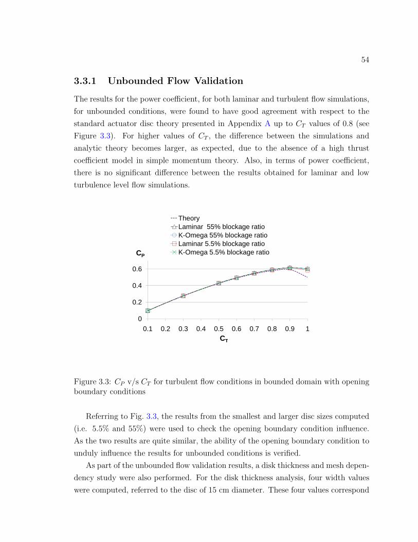
54

3.3.1 Unbounded Flow Validation

The results for the power coefficient, for both laminar and turbulent flow simulations,

for unbounded conditions, were found to have good agreement with respect to the

standard actuator disc theory presented in Appendix A up to CT values of 0.8 (see

Figure 3.3). For higher values of CT , the difference between the simulations and

analytic theory becomes larger, as expected, due to the absence of a high thrust

coefficient model in simple momentum theory. Also, in terms of power coefficient,

there is no significant difference between the results obtained for laminar and low

turbulence level flow simulations.

0.4

0.6

TheoryLaminar 55% blockage ratioK-Omega 55% blockage ratioLaminar 5.5% blockage ratioK-Omega 5.5% blockage ratioCP

0

0.2

0.4

0.1 0.2 0.3 0.4 0.5 0.6 0.7 0.8 0.9 1CT

Figure 3.3: CP v/s CT for turbulent flow conditions in bounded domain with openingboundary conditions

Referring to Fig. 3.3, the results from the smallest and larger disc sizes computed

(i.e. 5.5% and 55%) were used to check the opening boundary condition influence.

As the two results are quite similar, the ability of the opening boundary condition to

unduly influence the results for unbounded conditions is verified.

As part of the unbounded flow validation results, a disk thickness and mesh depen-

dency study were also performed. For the disk thickness analysis, four width values

were computed, referred to the disc of 15 cm diameter. These four values correspond

55

to a thicknesses of 5%, 1%, 0.5%, and 0.25% of the disc diameter respectively. The CP

was computed for the four cases and the results compared to the CP values expected

from theory (Appendix A). Table 3.1 presents the difference between the computed

CP and the theory value, for each disc thickness case, over a range of CT values.

CT 5 % diameter 1 % diameter 0.5 % diameter 0.25 % diameter

0.1 0.06 % 0.06 % 0.06 % 0.06 %0.3 0.24 % 0.23 % 0.22 % 0.22 %0.5 0.52 % 0.52 % 0.49 % 0.49 %0.7 1.19 % 1.15 % 1.07 % 1.07 %0.9 3.28 % 3.18 % 3.02 % 3.01 %

Table 3.1: ∆ CP (%) with respect theory value for different disc thickness

From this study, a disc thickness of 0.5 % of disc diameter was found to be

appropriate for the simulations, since at this width value the difference in CP values

with respect the theory became almost constant. Decreasing the disc thickness further

did not increase the accuracy of the results but did increase the simulation run times.

Regarding the mesh dependency study, a similar approach was used to determine

the best mesh configuration based on a tradeoff between speed and accuracy. A

structured mesh was defined for the unbounded domain. Since the main changes in

the velocity vector occur in the axial plane (perpendicular to the rotor plane), the

mesh of the sections aligned with the rotor plane was kept constant upstream and

downstream of the rotor, and only the mesh comprising the elements perpendicular

to the disc plane were changed to explore mesh dependency. The mesh in the axial

plane was defined starting with the smallest element sizes at the disc plane and then

increasing the element size upstream and downstream perpendicular to the disc plane.

The mesh inflation ratio at the disc proximity was set to a value of 1.1.

Four cases were run, as detailed in Table 3.2, and the results in terms of the

difference between CP from simulations and theoretical expected values are presented

in Table 3.3.

Based on the result obtained for the different configurations, presented in Ta-

ble 3.3, the mesh with 40 elements upstream and 50 elements downstream was found

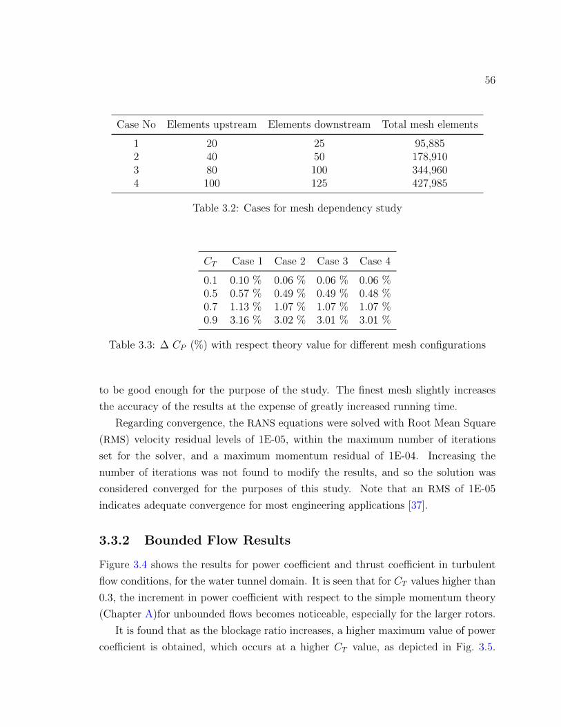
56

Case No Elements upstream Elements downstream Total mesh elements

1 20 25 95,8852 40 50 178,9103 80 100 344,9604 100 125 427,985

Table 3.2: Cases for mesh dependency study

CT Case 1 Case 2 Case 3 Case 4

0.1 0.10 % 0.06 % 0.06 % 0.06 %0.5 0.57 % 0.49 % 0.49 % 0.48 %0.7 1.13 % 1.07 % 1.07 % 1.07 %0.9 3.16 % 3.02 % 3.01 % 3.01 %

Table 3.3: ∆ CP (%) with respect theory value for different mesh configurations

to be good enough for the purpose of the study. The finest mesh slightly increases

the accuracy of the results at the expense of greatly increased running time.

Regarding convergence, the RANS equations were solved with Root Mean Square

(RMS) velocity residual levels of 1E-05, within the maximum number of iterations

set for the solver, and a maximum momentum residual of 1E-04. Increasing the

number of iterations was not found to modify the results, and so the solution was

considered converged for the purposes of this study. Note that an RMS of 1E-05

indicates adequate convergence for most engineering applications [37].

3.3.2 Bounded Flow Results

Figure 3.4 shows the results for power coefficient and thrust coefficient in turbulent

flow conditions, for the water tunnel domain. It is seen that for CT values higher than

0.3, the increment in power coefficient with respect to the simple momentum theory

(Chapter A)for unbounded flows becomes noticeable, especially for the larger rotors.

It is found that as the blockage ratio increases, a higher maximum value of power

coefficient is obtained, which occurs at a higher CT value, as depicted in Fig. 3.5.

57

0.60

0.80

1.00

Theory 9% Blockage ratio20% Blockage ratio 55% Blockage ratio5.5% Blockage ratio

CP

0.00

0.20

0.40

0.1 0.2 0.3 0.4 0.5 0.6 0.7 0.8 0.9 1.0CT

Figure 3.4: CP v/s CT for turbulent flow conditions in water tunnel domain

Note that optimal rotor performance for free-stream conditions occurs at a CT value

of approximately 0.89, thus these differences become important. This effect was also

mentioned by Garret, in the study of the efficiency of a tidal turbine operating in

its optimum conditions [42]. Table 3.4 presents the maximum value of the power

coefficient found for each blockage ratio in the CFD simulations.

Notice that as the blockage in the tunnel is increased, extra power needs to be

added to flow. Physically this is made possible in the experiments by extra pressure

being provided by the pump system to keep a constant flow rate at the inlet of the

water tunnel while performing the experiments. In a real tidal channel, increased

blockage would in fact retard the overall flow through the channel. Therefore Fig. 3.5

should not be interpreted as indicated that very high blockage ratios are advantageous

(there will be a unique optimum for each channel [42]).

3.3.3 Tunnel Wall Boundary Growth Effects

The effect of boundary layer growth was explored for a blockage ratio of 9%, which

represents the scaled rotor size within the water tunnel facility. The results are shown

in Fig. 3.6. For the case in which a no-slip condition was defined at the wall boundary,

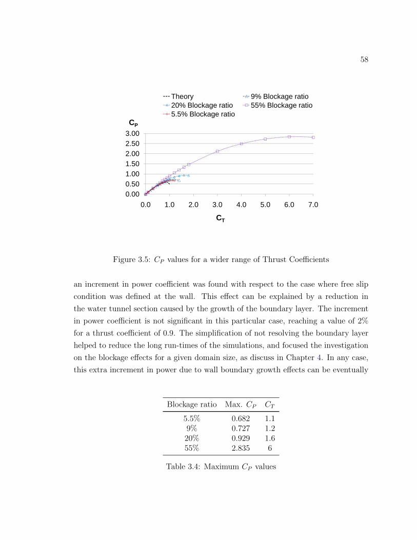
58

1.502.002.503.00

Theory 9% Blockage ratio20% Blockage ratio 55% Blockage ratio5.5% Blockage ratio

CP

0.000.501.001.50

0.0 1.0 2.0 3.0 4.0 5.0 6.0 7.0

CT

Figure 3.5: CP values for a wider range of Thrust Coefficients

an increment in power coefficient was found with respect to the case where free slip

condition was defined at the wall. This effect can be explained by a reduction in

the water tunnel section caused by the growth of the boundary layer. The increment

in power coefficient is not significant in this particular case, reaching a value of 2%

for a thrust coefficient of 0.9. The simplification of not resolving the boundary layer

helped to reduce the long run-times of the simulations, and focused the investigation

on the blockage effects for a given domain size, as discuss in Chapter 4. In any case,

this extra increment in power due to wall boundary growth effects can be eventually

Blockage ratio Max. CP CT

5.5% 0.682 1.19% 0.727 1.220% 0.929 1.655% 2.835 6

Table 3.4: Maximum CP values

59

incorporated to the final axial induction factor a-CP correction curve.

0.40

0.60

0.80

Free slip condition at the wall

Non-slip condition (B.Layer)CP

0.00

0.20

0.1 0.3 0.5 0.7 0.9 1.1 1.3

CT

Figure 3.6: Boundary layer effect for a rotor diameter 15 mm (9% blockage ratio)referenced to tunnel conditions

3.3.4 Reynolds Dependency Analysis

A set of simulations for turbines of different diameters and flow speeds were run to

explore the Reynolds wake dependency effects over a wider range of ReD. These

simulations, as detailed in Table 3.5, resulted in practical ReD ranging from 2x105

to 2x107, where ReD is defined based on disc diameter. The intent of these simula-

tions was to explore any Reynolds number effects in the viscous wake to verify the

assumptions of ReD independence in the CFD simulations.1 Clearly the actuator disc

simulations ignore any blade chord Reynolds number effects, which are known to be

important, but are a separate consideration to the wake dependency on ReD.

Simulations for each case detailed in Table 3.5 were run for different blockage

ratios. The change in power coefficient as defined in Eq. (4.4) was computed for each

case. Figure 3.7 presents the results for the power coefficient to thrust coefficient

1It is commonly asserted that wake dynamics are ReD in experimental campaigns.

60

Turbine diameter [m] Inlet velocity [m/s] ReD

0.15 2 2x105

0.15 150 2x107

1 3 2x106

10 3 2x107

Table 3.5: Turbine size and flow conditions for additional RANS simulations

relationship in turbulent flow conditions for the unbounded domain. For thrust co-

efficients up to 0.8 good agreement can be observed for the power coefficient with

respect the theory, for the whole range of Re. Also, there is no noticeable difference

between the power coefficient values obtained in the simulations for Re ranging from

105 to 107.

Figure 3.8 shows the increment in power coefficient with respect the unbounded

domain at CT = 8/9, as the blockage ratio varies, for different ReD conditions. There

is an expected positive trend; as the blockage ratio increases, the increment in CP also

becomes greater. With respect to the values of CP obtained for the same blockage

ratio and different Re numbers, there is only a subtle difference between the values,

less than 2 % in terms of CP increment that becomes noticeable at larger blockages

ratio values, such as 60 %. These results support the assumption that the mismatch

between full-scale and model scale Reynolds number do not affect wake development,

as these CFD simulations only simulate the wake behaviour.

61

0.4

0.5

0.6

0.7

CP Theory Re 2x10^5 (Disc 15 cm)

Re 2x10^7 (Disc 15 cm) Re 2x10^6 (Disc 1 m)

Re 2x10^7 (Disc 10 m)

CP

0

0.1

0.2

0.3

0 0.2 0.4 0.6 0.8 1CT

Figure 3.7: CP v/s CT , Unbounded domain

15%

20%

25%

30%

35%

Re 2x10^7 (Disc 10 m) Re 2x10^7 (Disc 15 cm)

Re 2x10^5 (Disc 15 cm) Re 2x10^6 (Disc 1 m)

∆∆∆∆ CP

0%

5%

10%

15%

0% 10% 20% 30% 40% 50% 60%

Blockage ratio [%]

Figure 3.8: CP increment v/s blockage ratio at CT = 8/9

62

Chapter 4

Tunnel Blockage Correction

Models

It is desirable in experimental testing to have larger scale models to achieve Reynolds

(Rec) similitude. However, for a large ratio of rotor swept area to tunnel cross-section

area, the walls of the water tunnel constrain the flow and increase the velocities

around the rotor. This in turn increases the forces and torques compared to open

water conditions, as depicted in Fig. 1.2, Chapter 1. Thus, the values acquired from

experiments performed in tunnel facilities must be corrected to unbounded conditions,

to accurately predict the performance of full size turbines. Available methodologies

for correcting results handle the tunnel interference by determining an equivalent free

stream velocity, and correlating this value to thrust coefficient to finally correct the

measured power coefficient.

Hence, standard blockage correction techniques require measurement of rotor

thrust to correct power coefficients for bounded testing domains. Due to the small

forces and compact nature of the testing rig developed in this thesis, accurate thrust

measurement is not possible. This chapter therefore presents a methodology that uti-

lizes the velocity field data at the rotor plane obtained from the water tunnel test and

CFD simulations based on the actuator disk concept to account for blockage without

the requirement for thrust data. The velocity can be obtained with PIV or other tech-

niques, however PIV data is to be simultaneously utilized for wake characterization

and to estimated the average velocity at the disc plane, and so was made the basis of

the new correction technique.

In essence, the correction technique uses PIV measurements to compute an average

63

axial induction factor that can be related to the characteristic power coefficient. From

CFD simulations, the increment in CP is predicted for a given set of operational con-

ditions that represents the water tunnel setup. These CFD values then provide a a-CP

correction curve to be utilized for processing the experiment test data. Furthermore,

to investigate the validity of the conventional analytical expressions, a comparison is

made between analytical and CFD correction results for different operational condi-

tions and blockage ratios.

4.1 Thrust Based Analytical Models

One of the first tunnel correction methods was developed for propeller testing by

Glauert [20] in the late 1920’s. Glauert introduced the concept of equivalent free air

speed V ′ which would produce the same velocity at the disc, thrust and torque on the

rotor as those observed in the tunnel for the corresponding tunnel datum velocity U0.

In that model, the real and scale machines both rotate at the same angular velocity

thus giving different tip-speed ratios for free and tunnel conditions. For propellers,

the equivalent free stream velocity is normally less than the tunnel datum velocity,

whereas for energy extracting devices, such as wind and tidal turbines, this equivalent

freestream velocity is larger than the tunnel datum speed.

To find the equivalent free velocity V ′, based on the actuator disk approach, the

principles of momentum balance, force balance, and continuity are applied to the case

of the device rotating in the tunnel. Finally, an analytical expression correlating V ′,

inflow tunnel velocity U0, relative rotor/tunnel size, and thrust coefficient CT is found

and used to correct the testing data to unbounded conditions. This method, based

on the axial momentum theory, is still widely used and has been adapted for wind

turbine experimental testing corrections [19], accounting for negative thrust (relative

to propellers which in Glauert’s theory have positive thrust).

An improvement to the Glauert method was recently developed by Mikkelsen and

Sorensen for wind turbines [21, 43]. This method is also based on the axial momentum

theory and the concept of equivalent free stream velocity of Glauert [20], but a new

solution was presented to account for the wall blockage effects of flow expansion. This

method has the advantage of working with non-dimensional variables and obtaining

the corrected free stream velocity UC in a more straightforward procedure but still

64

requiring thrust measurements. Moreover, this methodology resolved the singularity

inherent in Glauert’s correction for a thrust coefficient of -1.

Regarding tidal turbines, as yet little has been developed to account for wall in-

terference in experimental testing. One good reference is provided by Bahaj [15] who

derived an analytical blockage correction for wake expansion applicable to experimen-

tal testing of tidal turbines. This analytical correction was derived using an actuator

disk model to represent the rotor of the turbine, and applying the principles of con-

tinuity and momentum and force balance on the water between the far upstream

and far downstream at the tunnel facility. An equivalent water speed UF , similar to

the equivalent free stream velocity V ′ determined by Glauert [20], was obtained by

applying an iterative procedure. Finally, experimental power and thrust coefficients,

as well as tip speed ratios are corrected as a function of the ratio of equivalent open

water speed to water tunnel velocity. The method is very similar to those developed

for wind turbines.

4.1.1 Momentum Based Model

The three analytic reference models cited above represent the propeller [20] or turbine

[15, 21, 43] by a disk plane that causes a uniform pressure drop as the flow goes across

it [1]. The flow field is assumed to be inviscid, irrotational, and incompressible over

the entire domain. Two separate regions are clearly defined as shown in Fig. 4.1; the

region inside the streamtube and the region between the streamtube and the walls of

the tunnel.

Far upstream, the flow is characterized by a uniform axial inlet velocity U0 and a

pressure p0. A stream tube with upstream area smaller than the disc bounds the flow

through the disk. As the flow approaches the disk, its velocity slows down, which

also causes expansion of the streamtube. This induced velocity can be described

by a speed variation factor a = 1 − u1U0

called the axial induction factor. At the

disk plane, a pressure drop (p+ − p−) is exerted to account for energy extraction,

and as a result of this the downstream flow inside the streamtube, called the wake,

proceeds with reduced pressure and reduced velocity, compared to the flow outside

the streamtube. In the far wake, it is assumed that the pressure has risen to match the

flow pressure outside the bounding streamline, and the wake has fully expanded. Very

far downstream viscous mixing combines exterior and interior flows. Refer to Fig. 4.1,

65

Uo

Uo

p3

u1u2

u3

p-Tp

C

Uo

po

A

W

p2 = p3

p-p+

Figure 4.1: Actuator disk model in a closed tunnel section

at the far wake p2 = p3 < p0 and u2 < u3. Clearly the distinct wake expansion then

mixing regions are an approximation to reality, but this standard theory has been

shown to be a reasonable analytic model.

Unlike what this simple theory dictates and from which the analytical corrections

[15, 20, 21, 43] were obtained, while performing experimental testing in a water tunnel,

the viscosity and the turbulence in the fluid will produce - to a greater or lesser

degree depending on the flow conditions - lateral flow mixing between the wake and

the region outside the streamtube. Additionally, the larger the blockage ratio and

the rotor load, the larger the increment in the axial induction factor, which leads to

smaller velocities in the wake and higher velocities downstream outside the streamtube

which eventually will cause the flow to mix into the streamtube. Also, for higher

thrust loads, a region with flow recirculation becomes visible within the wake. These

effects are accounted for in standard the BEM theory used to analyze rotors through

empirical CT models, as the simple momentum formulations of BEM theory break

down. Therefore, depending on the operational conditions of the turbine being tested,

and the relative rotor size to the tunnel cross sectional area, analytical expressions may

66

not give accurate corrections. This uncertainty motivates the current investigation to

determine the blockage ratio range in which analytical corrections can be satisfactorily

applied without incurring significant errors. In addition, rationalized bounds on model

size and testing thrust values are required.

4.2 Blockage Correction Model Development

The models presented by Glauert [20], Mikkelsen and Sorensen [21, 43], and Bahaj

[15], provide a correlation between CT and the ratio of equivalent open velocity (UC) to

tunnel velocity. This accounts for the change in loading and induced velocities, due to

wall interference in a testing tunnel, and can be used to correct the experimental data.

Once the theoretical corrected velocity is determined, by solving any of the methods

previously identified, the corrections to the experimental characteristic coefficients

are a straightforward mathematical calculation.

For a given CT obtained from thrust measurement in the test tunnel, there is a

corresponding correction factor that should be applied to get the equivalent character-

istic coefficient in open conditions. Corrections for the power and thrust coefficients

and the tip speed ratio λ, as noted in reference [15] are:

CP,unb = CP,wt

(U0

UC

)3

(4.1)

CT,unb = CT,wt

(U0

UC

)2

(4.2)

λunb = λwt

(U0

UC

)(4.3)

where U0 is the actual inlet velocity in the experiments, UC is the velocity corrected

to freestream conditions, CP,unb, CT,wt, and λunb correspond to the power coefficient,

thrust coefficient and tip speed ratio for unbounded domain, and CT,unb, CP,wt, and

λwt correspond to the power coefficient, thrust coefficient, and tip speed ratio obtained

in the tunnel facility.

It is important to notice that a difficulty arises in this process when thrust data

is not being acquired during testing. To address this issue, in the current work, CFD

simulations are used to estimate the corrected free stream velocity and to also provide

67

a correction curve relating the available experimental data and the corrected velocity,

as described in the following paragraphs.

Figure 4.2 shows the trend curve for CP versus CT for both domains, the water

tunnel and the unbounded region. ∆ is defined as the difference between the water

tunnel-power coefficient CP,wt and the unbounded-power coefficient CP,unb, for a given

CT value , as shown in Eq. (4.4). Note that CT is referenced to actual conditions in

both domains.

∆ = CP,wt − CP,unb (4.4)

Water tunnel

CP,unb

CP,wt

CP

∆

CT

Unbounded domain

Figure 4.2: Trend of CP v/s CT in water tunnel and unbounded domains

Thus, the power coefficients in the water tunnel and unbounded domains for a

given thrust coefficient can be expressed as in Eq. (4.5) and in Eq. (4.6), where Pwt

and Punb are the power extracted by the rotor in the water tunnel and unbounded

domain respectively.

68

CP,wt =Pwt

12ρAU3

0

(4.5)

CP,unb =Punb

12ρAU3

0

(4.6)

Since CP,wt > CP,unb, for a given CT value, it is clear that Pwt 6= Punb as defined

in Eq. (4.5) and Eq. (4.6). However, it is possible to define a corrected freestream

velocity UC that will produce the same thrust force at the rotor in the unbounded

domain as in the water tunnel, for a given velocity u1 across the disk, and when the

turbine is assumed to keep the same angular velocity [20]. Therefore, at these similar

conditions in the bounded and unbounded domains, the same torque and power are

generated.

For this corrected freestream velocity UC , the power in the water tunnel is the

same as the power in the unbounded domain Pwt = P ′unb, where P ′unb is the equivalent

power that the rotor would extract while running at the same rotational speed inserted

in a flow stream having a speed equal to the corrected free stream velocity UC [20].

Consequently, CP,unb can be rewritten as in Eq. (4.7), where CP,wt is found to be

proportional to CP,unb by a factor K3, as shown in Eq. (4.8). From CFD simulations,

the power coefficient for both the unbounded and water tunnel conditions can be

obtained for a range of thrust coefficients. Then, replacing the corresponding values

of CP,unb and CP,wt in Eq. (4.8) a correction factor K3, correlating power and thrust

coefficient, is estimated. Also, from CFD simulations an average axial induction factor

is computed for both the unbounded and tunnel domain, for the range of CT values.

As a result, there is a corresponding power coefficient CP , an axial induction factor

a, and a correction factor K3 associated with each given thrust coefficient CT . In

such way, a curve correlating axial induction factor and thrust coefficient is obtained,

providing the final axial induction factor/power coefficient correction curve that will

be utilized in the data correction for the experimental testing.

CP,unb =P ′unb

12ρAU3

C

(4.7)

CP,wt = CP,unb

(UCU0

)3

= CP,unbK3 (4.8)

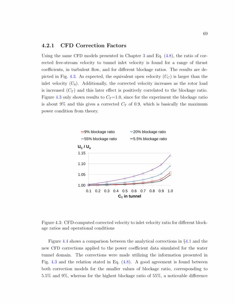
69

4.2.1 CFD Correction Factors

Using the same CFD models presented in Chapter 3 and Eq. (4.8), the ratio of cor-

rected free-stream velocity to tunnel inlet velocity is found for a range of thrust

coefficients, in turbulent flow, and for different blockage ratios. The results are de-

picted in Fig. 4.3. As expected, the equivalent open velocity (UC) is larger than the

inlet velocity (U0). Additionally, the corrected velocity increases as the rotor load

is increased (CT ) and this later effect is positively correlated to the blockage ratio.

Figure 4.3 only shown results to CT=1.0, since for the experiment the blockage ratio

is about 9% and this gives a corrected CT of 0.9, which is basically the maximum

power condition from theory.

1.10

1.15

9% blockage ratio 20% blockage ratio

55% blockage ratio 5.5% blockage ratio

UC / Uo

1.00

1.05

0.1 0.2 0.3 0.4 0.5 0.6 0.7 0.8 0.9 1.0CT in tunnel

Figure 4.3: CFD-computed corrected velocity to inlet velocity ratio for different block-age ratios and operational conditions

Figure 4.4 shows a comparison between the analytical corrections in §4.1 and the

new CFD corrections applied to the power coefficient data simulated for the water

tunnel domain. The corrections were made utilizing the information presented in

Fig. 4.3 and the relation stated in Eq. (4.8). A good agreement is found between

both correction models for the smaller values of blockage ratio, corresponding to

5.5% and 9%, whereas for the highest blockage ratio of 55%, a noticeable difference

70

appears between the analytical and CFD corrections. At the Betz limit condition,

the analytical expressions seem to overestimate the corrections by 7% and 20%, for a

blockage ratio of 20% and 55% respectively.

Finally, a correction curve based on axial induction factor a-CP is obtained for

a 9% blockage ratio that will be utilized to correct the experimental data. The

correction curve is depicted in Fig. 4.5b which provides information related to the

power coefficient increment expected for a given axial induction factor. Given that

the novel CFD correction method appears valid for higher blockage rations, future

experimental campaigns will include larger rotors with higher blockage to validate

this approach. For these cases, additional CFD data for higher CT could be used to

generate extended correction curves. The use of larger rotors would of course alleviate

on-blade Reynolds Rec number effects as well as provide higher forces which could

improve the signal-to-noise ratios of the torque measurements. Typically, optimal

operational conditions occur at an axial induction factor of 0.3, thus a potential 20%

increment in CP can be predicted for the experimental data, as seen in Fig. 4.5.

71

0.00

0.20

0.40

0.60

0.80

0.1 0.2 0.3 0.4 0.5 0.6 0.7 0.8 0.9 1.0

Theory Analytical correction

CFD correctionCP

5.5 % blockage ratio

0.00

0.20

0.40

0.60

0.80

0.1 0.2 0.3 0.4 0.5 0.6 0.7 0.8 0.9 1.0

Theory Analytical correction

CFD correction

CT

CP

5.5 % blockage ratio

0.00

0.20

0.40

0.60

0.80

0.1 0.2 0.3 0.4 0.5 0.6 0.7 0.8 0.9 1.0C

CP

9 % blockage ratio

0.00

0.20

0.40

0.60

0.80

0.1 0.2 0.3 0.4 0.5 0.6 0.7 0.8 0.9 1.0

Theory Analytical correction

CFD correction

CT

CP

5.5 % blockage ratio

0.00

0.20

0.40

0.60

0.80

0.1 0.2 0.3 0.4 0.5 0.6 0.7 0.8 0.9 1.0CT

CP

9 % blockage ratio

0.00

0.20

0.40

0.60

0.80

0.1 0.2 0.3 0.4 0.5 0.6 0.7 0.8 0.9 1.0CT

CP

20 % blockage ratio

0.00

0.20

0.40

0.60

0.80

0.1 0.2 0.3 0.4 0.5 0.6 0.7 0.8 0.9 1.0

Theory Analytical correction

CFD correction

CT

CP

5.5 % blockage ratio

0.00

0.20

0.40

0.60

0.80

0.1 0.2 0.3 0.4 0.5 0.6 0.7 0.8 0.9 1.0CT

CP

9 % blockage ratio

0.00

0.20

0.40

0.60

0.80

0.1 0.2 0.3 0.4 0.5 0.6 0.7 0.8 0.9 1.0CT

CP

20 % blockage ratio

0.00

0.20

0.40

0.60

0.80

0.1 0.2 0.3 0.4 0.5 0.6 0.7 0.8 0.9 1.0CT

CP

55 % blockage ratio

Figure 4.4: Comparison between analytical and CFD power coefficient corrections(all values corrected to free-stream, CT referred to tunnel conditions)

72

1.02

1.03

1.04

1.05

1.06

UC/U0

1

1.01

1.02

0 0.1 0.2 0.3

Axial induction factor in tunnel

(a) Ratio of corrected velocity to tunnel velocity v/s axial induction factor fora 9% blockage ratio

10%

15%

20%

∆∆∆∆ CP (%)

0%

5%

0 0.1 0.2 0.3Axial induction factor in tunnel

(b) Increment in power coefficient v/s axial induction factor for a 9% blockageratio

Figure 4.5: Correction curve for the experimental testing referenced to tunnel condi-tions

73

Chapter 5

Experimental Procedures and

Testing Campaigns

The ultimate goal of the experimental rig developed in this thesis is to enable testing

of a wide range of model rotors. These scaled models of HATTs and HAWTs will be

tested in a pressurized water tunnel at UVic in order to obtain characteristic power

coefficients and to address the need for detailed rotor wake measurements that will

be used to validate numerical prediction models.

The rig is specifically designed for the water tunnel having a cross sectional area

of 45 x 45 cm, with a maximum flow speed of 2 m/s. The nominal rotor diameter

designed for is 15 cm, so that the rotor swept area to the water tunnel section will be

approximately 9% to limit blockage effects as discussed in previous chapters. However,

as noted in Chapter 4, it will be possible to use larger rotors and correct for blockage

effects a posteriori. The inlet velocity of the water tunnel is limited to 2 m/s. In order

to maximize the blade Reynolds number, and to obtain different tip speed ratios, the

rotational speed will be therefore be varied. The velocity field in the near wake behind

the rotor will be acquired using PIVs technique with digital technology [44, 45].

This chapter first describes the specific objectives of the experimental campaigns

to be conducted with the rig. The experiment protocol utilized to carry out experi-

ments is described next, followed by results from the first set of results obtained from

the rig. The initial set of results presented in §5.5 (obtained by the author) turned

out to be not useful due to a number of difficulties realized after the test campaign.

The final set of results presented here were obtained by another co-op student, Peter

Root, with post-processing by the author.

74

5.1 Objectives of the experiment

The two specific objectives of this experimental rig are power output estimation and

the acquisition of the velocity field in the near wake behind the rotor, for different

operational conditions. Based on the power output estimation, the power coefficient

characteristic of the model run under different rotor speeds and inflow velocity in the

testing facility can be obtained. This characteristic is the fundamental performance

metric of any rotor. The vector velocity obtained in the near wake will provide

quantitative information to validate predictive codes. Additionally, as discussed in

Chapter 4, the same PIV data can be used to correct CP values obtained from the

experimental data.

5.1.1 Power output

For the power output estimation, the reaction torque of the motor driving the rotor

is measured. Having measured this reaction torque, the power output characteristic

of the model Pwt is estimated as follows:

Pwt = τrotorΩ (5.1)

where τrotor is the measured reaction torque, and Ω is the angular velocity of the

rotor. Once the power output is computed for a diverse range of rotational speeds,

the power coefficient characteristic of the model is calculated as shown in Eq. (5.2).

CP,wt =Pwt

1/2ρU3∞πR

2(5.2)

where CP,wt is power coefficient characteristic of the model running in the water

tunnel, ρ is the density of the water, and R the radius of the rotor.

The operational conditions can be expressed as defined in Eq. (2.1), where λ

relates the rotor speed and the tunnel inflow velocity, both characteristic factors of

the experiment being carried out. Notice that, later on, this experimental data must

be corrected to unbounded conditions as detailed in Chapter 4.

75

5.2 Experiment Protocol

The experiment will run the turbine placed inside a closed section water tunnel over

a range of rotational speeds. In such a way, it is possible to obtain a set of torque

measurements for a wide range of operational conditions. The results can then be

calculated and corrected for CP and λ to defined the characteristic curve of the rotor.

The first stage in the experiment, once the rig is placed into position with the

desired yaw condition for the particular test, is to fill the water tunnel until the

section is slightly pressurized. The pressurization is just enough to prevent air to

come into the tunnel while running the tunnel and the turbine.

Second, since the torque measurements are the net result of the forces on the

blades and the friction in the drivetrain of the rig, as discussed in §2.4, an important

step is to quantify the torque due to friction. This must be done without the rotor

blades installed, and a dummy hub installed instead of the rotor. The shaft is then

driven through the complete range of rotor speeds, and a correlation found between

friction torque and rotor speed. This friction torque will include bearing friction, the

dynamic seal on the shaft, and the belt system. The tests are run with the water

tunnel off, as the freestream fluid motion is unlikely to influence the frictions values

obtained (this has been verified experimentally). This frictional torque can then be

included in the final calculation of hydrodynamic torque, in order to isolate just the

component of torque due to the rotor. This friction estimation should be performed

every time the rotor is installed in the tunnel, and ideally before each round of testing.

Third, before starting up the rotor with the blades re-installed (the water tunnel

must be re-pressurized as well), the water tunnel is turned on and its flow speed is

gradually increased until reaching the value chosen for the set of measurements. Then,

the motor is run between 1 and 22 Revolutions per Second (RPS) for the data to be

acquired within that range. Notice that, as discussed in §2.4, the motor will operate as

a motor or generator depending on the net friction in the system, leading to turbine or

propeller operational conditions. This stage can be repeated for a number of different

inflow velocities in the water tunnel. The flow velocity is controlled by adjusting the

frequency of the pump system of water tunnel recirculation, as Table 5.1 shows. Note

that the advertised maximum flow speeds in some cases caused air leakage into the

tunnel, making it difficult for the tunnel to operate without air entrainment. This

can be avoided through additional pressurization (adding water) to the tunnel during

76

operation.

Finally, the water tunnel is turned off and the friction measurement is repeated.

It is important to open the drainage valve of the water tunnel when decreasing the

flow speed, otherwise the testing section is flooded and water will leak between the

sealed surfaces in contact with the top of the tank.

Frequency [Hz] Tunnel inflow velocity [m/s]15 0.6

25.5 0.935 1.3

Table 5.1: Pumping system frequencies and tunnel inflow velocity

5.3 Experimental Blade Sets

The blade sets used in these experiments had simple linear chord and twist distribu-

tions. The baseline blades used NACA63(2)-421 airfoil profiles. Inboard the blades

blended to a circular profile for attachment to the hub, which had a diameter of

19 mm. Over the active airfoil section of the blade, the chord tapered from 25 mm to

7 mm, and the blade was twisted 15 deg toward stall from zero pitch at the root. The

overall pitch angle of the blades in the rotors of the experiments was defined relative

to the pitch of the root section, with zero pitch aligning the root section in the plane

of rotation of the rotor.

For comparison to simulations, aero or hydrofoil properties at low Reynolds num-

bers can be input to the simulations, enabling comparison of the larger flow field

conditions and power outputs which are the primary area of interest for simulation

validation work. The blades produced for the rig using FDM technology (see §2.4.4)

inherently have a moderate surface roughness. Previous studies have shown that

fixed trip strips on the order of 0.25% chord located in the first 25% of the chord

can avoid the laminar separation type behaviour that limit airfoil performance at

Reynolds numbers around 1 × 104 to 1 × 105 [46]. The trip serves to prematurely

trigger turbulent transition, and this more energetic boundary layer is then able to

navigate the adverse pressure gradient on the airfoil without separation. In some cases

77

full transition may not occur at the trip strip, but reattachment can be facilitated

through laminar-turbulent transition over a laminar separation bubble.

Based on literature from the FDM manufacturer1, the typical surface roughness Ra

for the finest T10 tips (0.127 mm inch) is 0.015 mm. For typical chord lengths for the

rig’s blades around 10-30 mm, the surface roughness is on the order of 0.15% to 0.05%

chord, but distributed over the entire blade surface. The natural as-produced surface

roughness is therefore expected to be in the proper range to promote transition to

turbulence and hence achieve reasonable airfoil performance without massive laminar

separation regions or large laminar separation bubbles.

5.4 Measurement Error Estimation

Defining the error of a measurement as the difference between the measured value

and the true value of the variable to be measured, in experiments we can identify two

main categories of errors: systematic errors and random errors. Systematic errors

are fixed or bias errors; they are consistent and repeatable. It is assumed that if the

same measuring system is used in the same manner, and several measurements are

taken, the error will be the same each time. Random error are the scatter in the data

measured caused by a lack of repeatability in the output of the measuring system.

The random error in a single measurement corresponds to the difference between a

single reading and the average of all reading.

Notice that normally is not possible to know the error level in an experiment.

However, the uncertainty interval of the measurement can be estimated. The un-

certainty is defined as an estimation of the limits of error in the measurement [47].

Any experimental measurement will include some degree of uncertainty due to lack

of accuracy in the data acquisition equipment, random variation in the measurand,

sample size, etc.

Random uncertainty can be estimated using the expression given in Eq. (5.3):

UNC.RX = ±t SX√M

(5.3)

where UNC.RX is the random uncertainty estimation of the X measurement, SX is

the standard deviation of the sample, M is the sample size, and t is equal to 2 for

1www.fortus.com

78

a sample size larger than 30 and a confidence level of 95 %. Notice that random

uncertainty trends to zero as the sample size increases.

Systematic uncertainty does not depend on the sample size. In a particular vari-

able measured systematic uncertainties will remain constant if the experiment is re-

peated under the same conditions. These fixed errors can be estimated but not

eliminated from the measurement process.

In this study, uncertainty estimates were done to demonstrate the validity of the

results, and took into account the imprecision of the measurement (i.e. random

uncertainty) and an estimated maximum fixed error (i.e. systematic uncertainty) in

the torque data acquired.

Regarding PIV uncertainty, the main sources of error are related to the particle

displacement calculation. These errors mainly result from not choosing the most ap-

propriate method to extract the displacement peak from the correlation function, or

for distortion of the correlation function [48]. Low seeding density, velocity gradients,

interrogation cell resolution, etc. can cause errors in locating particles’ position from

the images and errors in velocity calculation. Fortily and Strykowsky [48] presented

a procedure that allows quantification of the bias and precision errors of DPIV in an

attempt to correct the systematic error presented in the mean displacement measure-

ments. However, no PIV data was acquired in this experiment thus, no uncertainty

analysis was be done for this measurand. As a reference, a similar experiment what

tested a scale model of a vertical turbine [49] in the same tunnel facility estimated the

total error in velocity was less than 2 %. However, values for spatial and temporal

resolution, appropriate for the operational conditions of this experiment, are needed

to more accurately estimate these errors.

5.4.1 Error estimation

In DAQ measurement systems there are several error sources, so called elemental er-

ror sources, generating either a random or systematic uncertainty. These elemental

errors can be arranged in 5 categories as ASME suggests [47]: calibration uncertain-

ties, data-acquisition uncertainties, data-reduction uncertainties, uncertainties due to

method and other uncertainties. This grouping has the sole purpose of identifying

and comparing uncertainties in measurements. In the end the elemental uncertainties

79

are combined by using the square root of the sum of the squares (RSS) to obtain the

total uncertainty [47].

The standard calibration process done at the factory is intended to minimize

resulting systematic errors, however there are some residual errors, leading to sys-

tematic uncertainties. Example of these calibration uncertainties are hysteresis and

nonlinearity. In the experiment performed, there are two instruments involved: the

torque cell and the NI 9237 module for torque measurement (§2.5).

Table 5.2 presents a summary of the sources of elemental error and uncertainties of

the measurements associated with each instrument, based on technical specifications

provided by the vendor.

Instrument Elemental Error Uncertainty (%)

Torque Cell Non linearity 0.1Torque Cell Repeatibility 0.05Torque Cell Hysteresis 0.04NI 9237 Gain error 0.2

Table 5.2: Uncertainties of measurement

Systematic and random uncertainty are combined by using the square root of the

sum of the squares (RSS) to obtain the total uncertainty. Notice that, because of

the large size of the sample (i.e. greater than 10, 000), the random uncertainty is

estimated to be zero. Then, the total uncertainty estimates result in approximated ±0.23%, obtained as in Eq. (5.4), where UNC is the total uncertainty estimate. This

means a maximum possible error of ± 0.0023 Nm for any given measurement. As

this error level is so small, error bars are not shown on any of the results plots, as

they are too small to be seen.

UNC =√

0.12 + 0.052 + 0.042 + 0.22 (5.4)

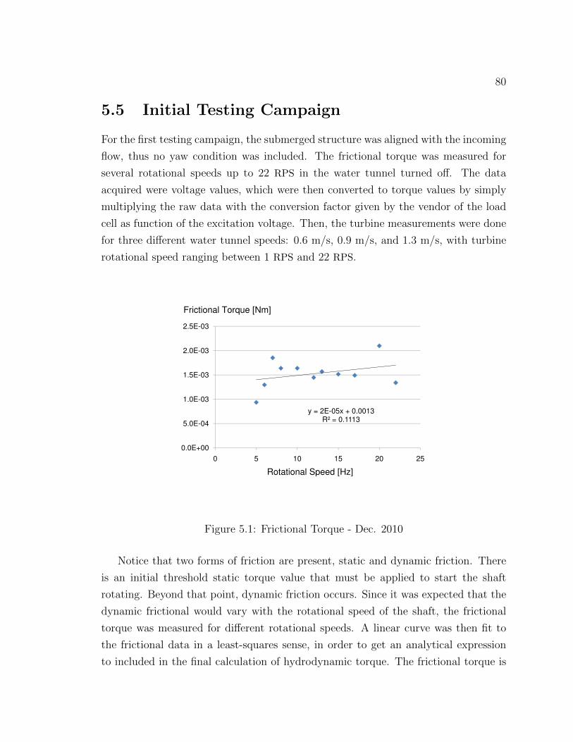
80

5.5 Initial Testing Campaign

For the first testing campaign, the submerged structure was aligned with the incoming

flow, thus no yaw condition was included. The frictional torque was measured for

several rotational speeds up to 22 RPS in the water tunnel turned off. The data

acquired were voltage values, which were then converted to torque values by simply

multiplying the raw data with the conversion factor given by the vendor of the load

cell as function of the excitation voltage. Then, the turbine measurements were done

for three different water tunnel speeds: 0.6 m/s, 0.9 m/s, and 1.3 m/s, with turbine

rotational speed ranging between 1 RPS and 22 RPS.

1.0E-03

1.5E-03

2.0E-03

2.5E-03

Frictional Torque [Nm]

y = 2E-05x + 0.0013R² = 0.1113

0.0E+00

5.0E-04

1.0E-03

0 5 10 15 20 25

Rotational Speed [Hz]

Figure 5.1: Frictional Torque - Dec. 2010

Notice that two forms of friction are present, static and dynamic friction. There

is an initial threshold static torque value that must be applied to start the shaft

rotating. Beyond that point, dynamic friction occurs. Since it was expected that the

dynamic frictional would vary with the rotational speed of the shaft, the frictional

torque was measured for different rotational speeds. A linear curve was then fit to

the frictional data in a least-squares sense, in order to get an analytical expression

to included in the final calculation of hydrodynamic torque. The frictional torque is

81

plotted in Fig. 5.1. In this first set of runs, frictional torque turned out to be of the

same order of magnitude as the turbine torque for rotational speeds up to 12 RPS.

-1,6

-1,4

-1,2

-1,0

-0,8

-0,6

-0,4

-0,2

0,00 5 10 15 20

0.6 m/s 0.9 m/s 1.3 m/sCP

Figure 5.2: CP v/s λ Results Dec. 2010

The blades of the rotor were then installed at 0 pitch angle relative to the blade

roots. Unfortunately, as seen in Fig. 5.2, the measurements obtained in this first cam-

paign were not useful in terms of characterizing turbine performance. Negative CP

values obtained confirmed the rotor was adding energy to the flow, not extracting as

expected for turbine rotor behaviour. The rotor operating as a propeller is explained

due to misalignment of the blade root, which resulted in a large negative pitch at

the tip and consequently, negative angles of attack accelerating the flow downstream

(propeller) rather than retarding it (turbine). This illustrates the utility of the mo-

tor/generator approach, so both turbine and propeller can be tested at constant λ.

5.6 Second Testing Campaign

As a result of the lessons learning during the first testing campaign by the author,

a second testing campaign was performed by a co-op student, Peter Root, who re-

designed the blade roots and achieved proper pitch alignment. The tests were re-run

82

with 1X and 1.5X blades, [50], again with NACA63(2)-4XX airfoil profiles. where

the size scaling is defined in terms of chord and blade radius length. The 1.0X and

1.5X blade size designations refer to linearly scaled blades, with the 1.0X blade size

corresponding to blades of 75 mm radius length, root chord of 25 mm and tip chord

of 7 mm. The overall twist of the blade was kept constant.

Different flow conditions, blade sizes and surface roughness effects were explored

in this set of experiments. Measurement were taken at a combination of low tunnel

velocity (0.6 to 1.3 m/s) and high tunnel velocity (1.5 to 1.9 m/s); ‘smooth’ and

‘rough’ blade surfaces, for both the 1.0X and 1.5X blade sizes.

The ‘rough’ blades were produced using T12 FDM tips (see §2.4.4), while the

‘smooth’ blades were produced using T10 tips. The 1.5X blade was obtained by

scaling the 1.0X blade up by 50%. Also, BEM simulations were run following the

methodology developed by Crawford [51], to be used for experimental results com-

parison. The BEM code used is typical of design codes used for kinetic turbines. Lift

and drag 2D airfoil coefficients were estimated using the XFoil software2 [52], with

forced transition at two chord locations, 10 %c and 30 %c. Forced transition was used

to reflect the flow conditions on the rough blade surfaces, and because free-transition

was found to predict massive separation at the lower Reynolds numbers tested, even

though overall rotor performance was not indicative of massive separation.

5.6.1 Operational Conditions

Figures 5.3 and 5.4 illustrate the α and Re operational range respectively, along

the blade, for both the 1.0X and 1.5X sized blades. The results are from the BEM

simulations where α is defined as the angle of attack determined form the incident

resultant velocity in the cross-sectional plane of the airfoil.

This second test campaign also faced inconsistent results for power and CP values.

It was first found that signal to noise ratio is low for the slow tunnel speeds, because

torque values measured were quite close to friction torque levels. This can be improved

by increasing inflow speeds [50]. Thus, the following test runs were performed with the

tunnel running at 1.5 m/s, 1.7 m/s and 1.9 m/s tunnel inflow velocity, corresponding

to 40, 45, and 50 Hz pumping frequencies, respectively, as indicated in Table 5.3.

2XFoil solves a coupled inviscid-viscid problem with boundary layer equations for 2D airfoils.This allows for good prediction of lift/drag performance across a range of Reynolds numbers, up toconditions nearing stall where the approach becomes invalid as gross separation occurs.

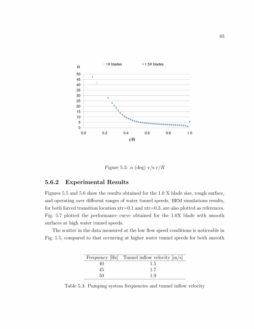
83

20

25

30

35

40

45

50

1X blades 1.5X bladesα

0

5

10

15

20

0.0 0.2 0.4 0.6 0.8 1.0

r/R

Figure 5.3: α (deg) v/s r/R

5.6.2 Experimental Results

Figures 5.5 and 5.6 show the results obtained for the 1.0 X blade size, rough surface,

and operating over different ranges of water tunnel speeds. BEM simulations results,

for both forced transition location xtr=0.1 and xtr=0.3, are also plotted as references.

Fig. 5.7 plotted the performance curve obtained for the 1.0X blade with smooth

surfaces at high water tunnel speeds.

The scatter in the data measured at the low flow speed conditions is noticeable in

Fig. 5.5, compared to that occurring at higher water tunnel speeds for both smooth

Frequency [Hz] Tunnel inflow velocity [m/s]40 1.545 1.750 1.9

Table 5.3: Pumping system frequencies and tunnel inflow velocity

84

3.E+04

4.E+04

5.E+04

6.E+04

7.E+04

8.E+04

1X Blades 1.5X BladesRe

0.E+00

1.E+04

2.E+04

3.E+04

0.0 0.2 0.4 0.6 0.8 1.0

r/R

Figure 5.4: Re v/s r/R

and rough blade surfaces. Also, measurements from high tunnel velocities with rough

surfaces seems to have better performance curve agreement with BEM simulations

than the experimental data for smooth-surfaced blades. The smooth surface blade

results show lower CP peaks compared to the rough surface data, at the same con-

ditions. There is also a clear shift in the CP vs. λ characteristic between the BEM

simulations and the experimental results. The differences are likely related to Re

number effects on the blade section characteristics, however the shift in performance

curves with respect to expected simulation results are not fully explained by his com-

parison.

5.6.3 Surface Roughness and Reynolds Number Effects

In order to explore and understand discrepancies due to Re and surface roughness,

Fig. 5.8 plots the results for the 1.0X and 1.5X blade sizes, both smooth surfaces, at

higher tunnel speeds.

It is instructive to look at the airfoil behaviour for an explanation. Figures 5.9

and 5.10 present predicted 2D lift coefficients over a range of angles of attack at

85

-0,3

-0,2

-0,1

0

0,1

0,2

0,3

0,4

0 1 2 3 4

1X rough 1.3 m/s 1X rough 0.9 m/s 1X rough 0.6 m/s

BEM 1X xrt03 1.3 m/s BEM 1X xrt03 0.9 m/s BEM 1X xrt03 0.6 m/s

BEM 1X xrt01 1.3 m/s BEM 1X xrt01 0.9 m/s BEM 1X xrt01 0.6 m/sCP

Figure 5.5: CP v/s λ at low water tunnel velocity (rough)

different Re, for transition forced at 10 % and 30 % chord respectively. Here xtr is

defined as the location for forced transition in terms of percentage of the chord length

starting from the leading edge of the airfoil section. At a Re of 1 × 105, there is a

bump in the curve between 12 degree and 14 degree data because the transition point

moves upstream of the 0.3c fixed transition point. The flow over the airfoil becomes

turbulent earlier, delaying laminar separation, thus reducing drag and increasing lift.

Then, for even higher angles of attack, turbulent separation grows and drag increases.

This situation is depicted in Figs. 5.11 and 5.12, at xtr = 0.1 and xtr = 0.3.

These predicted airfoil performance curves explain to some degree the higher CP

values for the rough blades surface compared to the smooth blades. As shown in

Figs. 5.3 and 5.4, the operational Re are in the 3× 104 to 7× 104 range and generally

below stall. Over those ranges, the 0.1c transition location curves (representative of

rough blades) generally have better performance in terms of drag compared to the

0.3c transition location curves (representative of smooth blades). Therefore, although

the BEM results to not predict large differences between bladesets, the experimental

data suggests that the airfoil performance is quite sensitive over this Reynolds num-

ber range, and to the surface roughness. The better performance of the smooth 1.5X

86

-0,3

-0,2

-0,1

0

0,1

0,2

0,3

0,4

0 1 2 3 4

1X rough 1.9 m/s 1X rough 1.7 m/s 1X rough 1.5 m/s

BEM 1X xrt03 1.9 m/s BEM 1X xrt03 1.7 m/s BEM 1X xrt03 1.5 m/s

BEM 1X xrt01 1.9 m/s BEM 1X xrt01 1.7 m/s BEM 1X xrt01 1.5 m/sCP

Figure 5.6: CP v/s λ at high water tunnel velocity (rough)

blades relative to the smooth 1X blades indicate a significant Re effect, given the

surfaces have similar roughness. Comparing the rough and smooth 1X blade results

in Figs. 5.6 and 5.7 respectively, the rough results are clearly superior in terms of per-

formance, again lending support to the hypothesis that rougher blade delay laminar

separation effects and enhance performance at these low Re numbers.

5.6.4 Estimation of Blockage Effects

It is also important to notice that increasing blade size lead to improved full size

turbine representation (larger Re), but also affects the measurements due to wake

expansion, and hence blockage effects must be explored too. Unfortunately, there was

no PIV data available to make a proper correction to experimental data accounting

for the induced velocity using the procedures developed in Chapter 4. However, a

rough CFD correction can be made, based on the methodology presented in Chapter 4,

considering lower and high thrust loads exerted by the rotor.

For the 15 cm rotor diameter (1.0X blade)the blockage ratio is about 9%. Two

correction factors K = UC/U0 are taken from the CFD simulations, Fig. 4.3, the first

for a low CT (e.g. 0.1) and the second for a high CT values (e.g. 1.0). In such a

87

-0,3

-0,2

-0,1

0

0,1

0,2

0,3

0,4

0 1 2 3 4

1X smooth 1.9 m/s 1X smooth 1.7 m/s 1X smooth 1.5 m/s

BEM 1X xrt03 1.9 m/s BEM 1X xrt03 1.7 m/s BEM 1X xrt03 1.5 m/s

BEM 1X xrt01 1.9 m/s BEM 1X xrt01 1.7 m/s BEM 1X xrt01 1.5 m/sCP

Figure 5.7: CP v/s λ at high water tunnel velocity (smooth)

way, CFD correction bounds are plotted in Figs. 5.13 to 5.15 over the experimental

data for the 1.0X rough blade surface, the 1.0X smooth blade surface, and the 1.5X

smooth blade surface, for the water tunnel running at 50 Hz (1.7 m/s flow velocity).

These bounds on the corrections that should be applied to the data in the absence

of PIV data. This is true even at the relatively small 9% blockage ratio. It also

appears that some of the discrepancy between the 1X and 1.5X blades in Fig. 5.8 can

be explained by the higher blockage for the 1.5X blades not being accounted for in

the absence of PIV data . This suggests that the Rec effects may not be as dramatic

as initially suggested by the uncorrected performance curves.

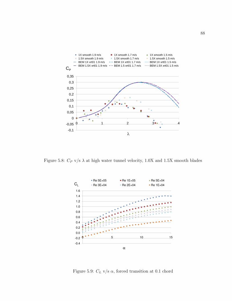
88

-0,1

-0,05

0

0,05

0,1

0,15

0,2

0,25

0,3

0,35

0 1 2 3 4

1X smooth 1.9 m/s 1X smooth 1.7 m/s 1X smooth 1.5 m/s1.5X smooth 1.9 m/s 1.5X smooth 1.7 m/s 1.5X smooth 1.5 m/sBEM 1X xrt01 1.9 m/s BEM 1X xrt01 1.7 m/s BEM 1X xrt01 1.5 m/sBEM 1.5X xrt01 1.9 m/s BEM 1.5 xrt01 1.7 m/s BEM 1.5X xrt01 1.5 m/s

CP

Figure 5.8: CP v/s λ at high water tunnel velocity, 1.0X and 1.5X smooth blades

0.6

0.8

1.0

1.2

1.4

1.6

Re 5E+05 Re 1E+05 Re 5E+04

Re 3E+04 Re 2E+04 Re 1E+04CL

-0.4

-0.2

0.0

0.2

0.4

0 5 10 15

α

Figure 5.9: CL v/s α, forced transition at 0.1 chord

89

0.6

0.8

1.0

1.2

1.4

1.6

Re 5E+05 Re 1E+05 Re 5E+04

Re 3E+04 Re 2E+04 Re 1E+04CL

-0.4

-0.2

0.0

0.2

0.4

0 5 10 15

α

Figure 5.10: CL v/s α, forced transition at 0.3 chord

0.6

0.8

1.0

1.2

1.4

1.6

Re 5E+05 Re 1E+05 Re 5E+04

Re 3E+04 Re 2E+04 Re 1E+04CL

-0.4

-0.2

0.0

0.2

0.4

0.6

0.00 0.05 0.10 0.15 0.20

CD

Figure 5.11: CD v/s CL xtr=0.1

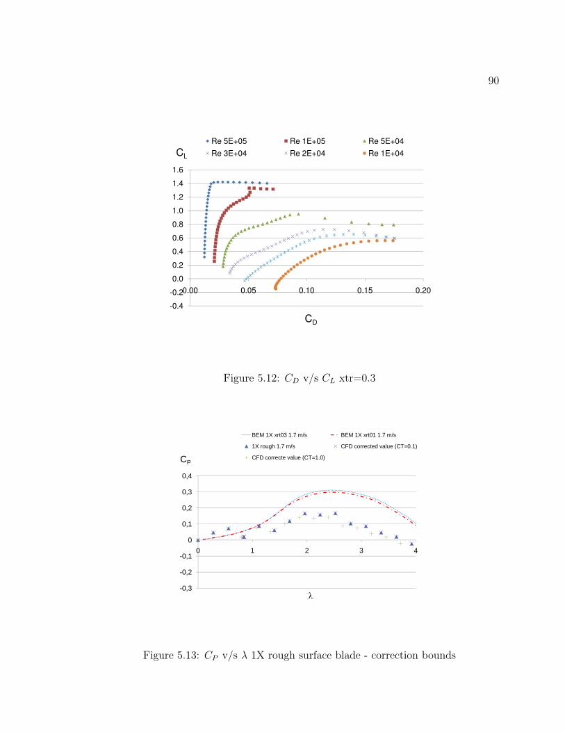
90

0.6

0.8

1.0

1.2

1.4

1.6

Re 5E+05 Re 1E+05 Re 5E+04

Re 3E+04 Re 2E+04 Re 1E+04CL

-0.4

-0.2

0.0

0.2

0.4

0.00 0.05 0.10 0.15 0.20

CD

Figure 5.12: CD v/s CL xtr=0.3

-0,3

-0,2

-0,1

0

0,1

0,2

0,3

0,4

0 1 2 3 4

BEM 1X xrt03 1.7 m/s BEM 1X xrt01 1.7 m/s

1X rough 1.7 m/s CFD corrected value (CT=0.1)

CFD correcte value (CT=1.0)CP

Figure 5.13: CP v/s λ 1X rough surface blade - correction bounds

91

-0,3

-0,2

-0,1

0

0,1

0,2

0,3

0,4

0 1 2 3 4

BEM 1X xrt03 1.7 m/s BEM 1X xrt01 1.7 m/s

1X smooth 1.7 m/s CFD corrected value (CT=0.1)

CFD correcte value (CT=1.0)CP

Figure 5.14: CP v/s λ 1X smooth surface blade - correction bounds

-0,3

-0,2

-0,1

0

0,1

0,2

0,3

0,4

0 1 2 3 4

BEM 1.5X xrt03 1.7 m/s BEM 1.5X xrt01 1.7 m/s

1.5X smooth 1.7 m/s CFD corrected value (CT=0.1)

CFD correcte value (CT=1.0)CP

Figure 5.15: CP v/s λ 1.5X rough surface blade - correction bounds

92

Chapter 6

Conclusions

Although it was not possible to complete final testing using PIV equipment during

the course of this thesis, a number of achievements were made. A rotor rig was

designed and tested, which when coupled with PIV measurements will provide high-

accuracy data using small-scale blade sets, enabling a large testing campaign. A set

of testing procedures were developed, including a PIV-based correction routine, that

will enable proper post-processing of the results to account for blockage effects. The

initial set of experiments has also highlighted the key areas needing refinement to

enable comparison of simulation and experimental results.

6.1 Rig Design

The design of the test rig was a comprehensive task, which included consideration of

scaling issues to achieve appropriate scale models that maximize chord Re without

compromising the reliability of the experimental data acquired because of blockage

effects. FEM modelling of the structure was completed to avoid coupling of vibrations

in the system and deformations of the rig support and sting beyond limits predefined.

The mechanical design itself meet several conditions both required and desirable for

testing purposes. The features of the rig are that it: minimizes the disturbance of

flow, allowing testing in yawed flow conditions up to 45 , and providing control over

operational conditions; it has an interchangeable hub that allows varying size rotors;

and it is a rig that can be added to by other SSDL researchers as future requirements

arises. Most notably, the rig could be improved by automation of the yaw system for

future tests.

93

6.2 Computational Fluid Dynamic Simulations

This research developed a methodology for wall interference corrections, based on CFD

simulations, that can be applied to find a correction curve for the experimental data

acquired in tunnel testing facilities. This curve correlates the average axial induction

factor (a) and the power coefficient (CP ) in the water tunnel, and an explicit curve

a-∆CP is derived to correct the dimensionless water tunnel power coefficient (CP,wt)

to freestream conditions.

An interesting outcome is that CFD results and analytical expressions present

good agreement (less than 5% difference) for blockages ratios up to 10%. For higher

ratios of swept rotor area to tunnel section, analytical expressions - based on the axial

momentum theory - seem to underestimate the power coefficient in the water tunnel,

which leads to higher analytical correction factors compared to that obtained from

CFD simulations.

The results of the wake Reynolds dependency study show the simulations turned

out to be Reynolds independent, which allow extrapolating the results of the model

to real operation conditions of the full size turbine.

6.3 Experimental Study

An experiment protocol was developed to acquire torque measurements for different

operational conditions in order to finally obtain the performance curve of tip speed

ratio to characteristic power coefficient.

Two testing campaigns have been carried out so far. The first set of experimental

data revealed an error in the alignment of the blade root. The rotor was operating

as a propeller rather than a turbine; hence, it was not possible to use the acquired

information to characterized the turbine behaviour. However, the testing capability

of the rig was successfully verified, and the data acquisition hardware allowed for

controlled operational conditions as needed.

The second testing campaign provided more useful results. As first insight, mea-

surements at low torque seems to be easily disturbed by other signals. Comparison of

data for each blade set across a range of higher water tunnel speeds show consistent

results. Comparison between blade sets of different sizes and similar roughness do

however likely show some Re dependency, however the bounds on the tunnel blockage

94

corrections to the data indicate that this effect may be dominant over Re dependency.

In any case, the CP results of smooth blade surfaces are lower than CP values obtained

from rough blades. Also, the best performance curves from simulation correspond to

rough blades at higher water tunnel velocities. It is clear that blade surface is a key

factor in the blade performance. Roughness significantly affects flow separation onset

on the airfoil profile, causing an earlier transition to turbulence and drag reduction

for angles of attack up to approximately 14 degree at 1E + 05 Re.

6.4 Future Work

It is obvious from the results presented in this thesis that in order to compare simu-

lation and experimental results, the low Reynolds number performance of the airfoils

to be used on the blade sets must be ascertained. The effect of roughness, includ-

ing manufacturing procedures and setup, must be a part of the characterization. To

this end, the additional experimental apparatus under construction in the SSDL is

required to experimentally measure 2D airfoil performance, as analysis codes such as

XFoil have ambiguous parameters and must be validated to use predictively.

Obviously the next step in the rig testing campaign is to integrated the PIV system,

and acquire simultaneous torque and PIV data. With this extra data, the mechanical

data can be properly corrected. Furthermore, the wake structure information will be

invaluable in validating rotor computation models, once accurate 2D airfoil data is

obtained. In the longer term, new blade designs can be constructed and tested on

the rig to validate performance of a wide range of kinetic turbine designs.

95

Bibliography

[1] T. Burton and D. Sharpe, Wind Energy Handbook. John Wiley & Sons, 2001.

ix, xi, 3, 12, 14, 15, 16, 64, 101

[2] F. Massouh and I. Dobrev, “Exploration of the vortex wake behind a wind tur-

bine rotor,” Journal of Physics, no. Series75-012036, 2007. 1, 12, 16, 41

[3] L. J. Vermeer, J. N. Sorensen, and A. Crespo, “Wind turbine wake aerodynam-

ics,” Progress in Aerospace Science, vol. 39, pp. 467–510, 2003. 1, 5, 9, 11, 13,

46

[4] A. Bahaj and L. Myers, “Analytical estimates of the energy yield potential from

the alderney race (channel islands) using marine current energy converters,”

Renewable Energy, vol. 29, pp. 1931–1945, 2004. 2

[5] J. King and T. Tryfonas, “Tidal power stream power technology - state of art,”

IEEE, 2009. 2, 3

[6] Tidal Generation Ltd., “Tidal generation.” 2

[7] Nova Scotia Power, “In-stream tidal turbine project overview.” 3

[8] J. S. Carlton, Marine Propellers and Propulsion. Elsevier, 2nd edition ed., 2007.

3

[9] L. Blunden and A. Bahaj, “Initial evaluation of tidal stream energy resources at

portland bill, uk,” Renewable Energy, vol. 31, pp. 121–132, 2006. 4

[10] I. Bryden, T. Grinsted, and G. Melville, “Assessing the potential of a simple tidal

channel to deliver useful energy,” Applied Ocean Research, vol. 26, pp. 198–204,

2004. 4

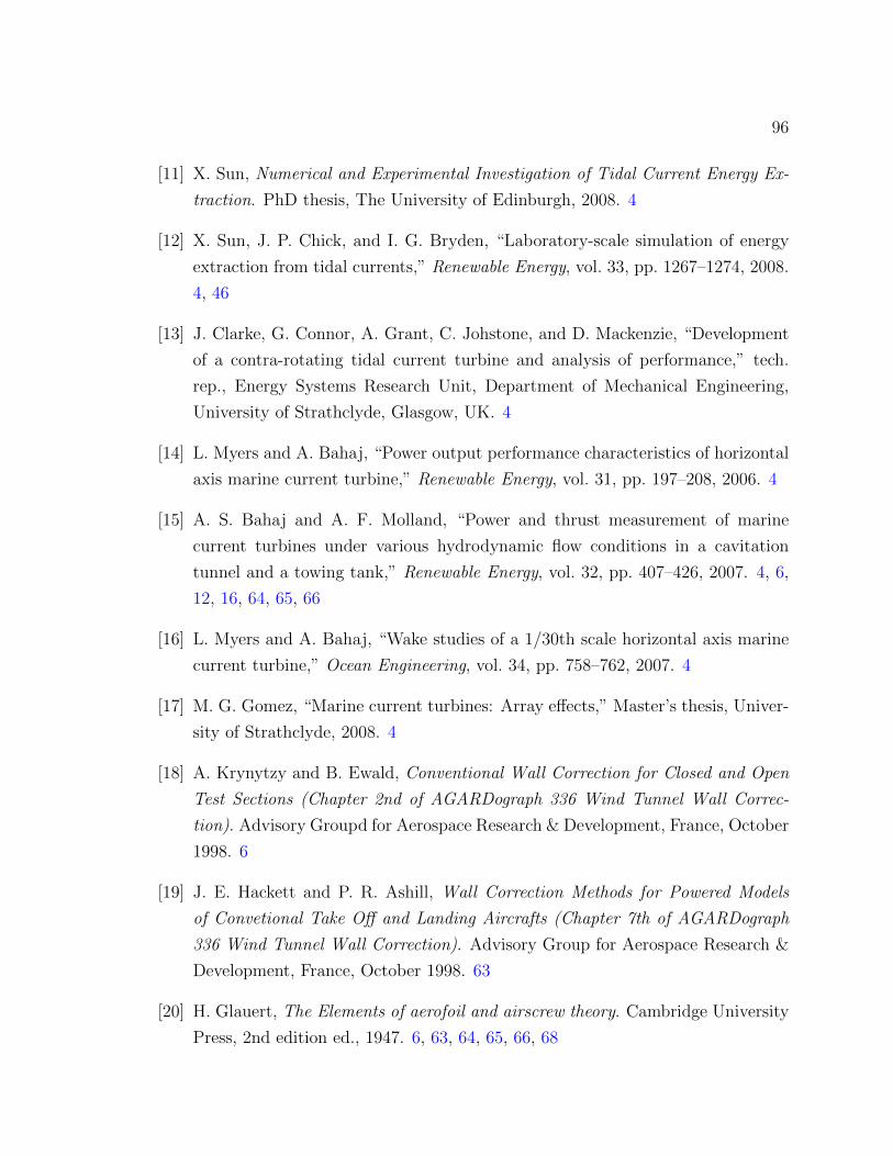
96

[11] X. Sun, Numerical and Experimental Investigation of Tidal Current Energy Ex-

traction. PhD thesis, The University of Edinburgh, 2008. 4

[12] X. Sun, J. P. Chick, and I. G. Bryden, “Laboratory-scale simulation of energy

extraction from tidal currents,” Renewable Energy, vol. 33, pp. 1267–1274, 2008.

4, 46

[13] J. Clarke, G. Connor, A. Grant, C. Johstone, and D. Mackenzie, “Development

of a contra-rotating tidal current turbine and analysis of performance,” tech.

rep., Energy Systems Research Unit, Department of Mechanical Engineering,

University of Strathclyde, Glasgow, UK. 4

[14] L. Myers and A. Bahaj, “Power output performance characteristics of horizontal

axis marine current turbine,” Renewable Energy, vol. 31, pp. 197–208, 2006. 4

[15] A. S. Bahaj and A. F. Molland, “Power and thrust measurement of marine

current turbines under various hydrodynamic flow conditions in a cavitation

tunnel and a towing tank,” Renewable Energy, vol. 32, pp. 407–426, 2007. 4, 6,

12, 16, 64, 65, 66

[16] L. Myers and A. Bahaj, “Wake studies of a 1/30th scale horizontal axis marine

current turbine,” Ocean Engineering, vol. 34, pp. 758–762, 2007. 4

[17] M. G. Gomez, “Marine current turbines: Array effects,” Master’s thesis, Univer-

sity of Strathclyde, 2008. 4

[18] A. Krynytzy and B. Ewald, Conventional Wall Correction for Closed and Open

Test Sections (Chapter 2nd of AGARDograph 336 Wind Tunnel Wall Correc-

tion). Advisory Groupd for Aerospace Research & Development, France, October

1998. 6

[19] J. E. Hackett and P. R. Ashill, Wall Correction Methods for Powered Models

of Convetional Take Off and Landing Aircrafts (Chapter 7th of AGARDograph

336 Wind Tunnel Wall Correction). Advisory Group for Aerospace Research &

Development, France, October 1998. 63

[20] H. Glauert, The Elements of aerofoil and airscrew theory. Cambridge University

Press, 2nd edition ed., 1947. 6, 63, 64, 65, 66, 68

97

[21] J. Sorensen and R. Mikkelsen, “Wall correction model for wind tunnel with open

test section,” AIAA, vol. 44, pp. 1890–1894, August 2006. 6, 63, 64, 65, 66

[22] C. Lartiga and C. Crawford, “Actuator disk modeling in support of tidal turbine

rotor testing,” in 3rd International Conference on Ocean Energy, (Bilbao, Spain),

Oct. 6–8 2010. 7

[23] C. Lartiga and C. Crawford, “Water tunnel rotor testing with post processing

based on PIV measurements,” in Proceedings of the ASME 2010 International

Mechanical Engineering Congress & Exposition (IMECE2010), (Vancouver, BC),

Nov. 12–18 2010. 7, 9

[24] B. Rawlings, V. Klaptocz, C. Crawford, C. Lartiga, M. Shives, M. Sireli, and

M. Alidadi, “Assessment of blockage effects on tidal energy converter perfor-

mance,” tech. rep., Nova Scotia Power Inc., Halifax, NS, Feb. 2011. 7

[25] A. Pope, W. H. Rae, and J. B. Barlow, Low-Speed Wind Tunnel Testing. John

Wiley& Sons, 3rd edition ed., 1999. 15, 16

[26] J. Whale and C. Anderson, “An experimental and numerical study of the vor-

tex structure in a wake of a wind turbine,” Journal of Wind Engineering and

Industrial Aerodynamic, vol. 84, pp. 1–21, 2000. 16

[27] H. Fernando, “Designing a water tunnel rotor dynamometer,” tech. rep., Depart-

ment of Mechanical Engineering, University of Victoria., 2010. 18, 22

[28] Ansys Inc., Ansys Help. ANSYS, 12 ed., 2010. 18, 20, 109

[29] D. L. Logan, A first course in the finite element method. CL Engineering, 4th ed.,

July 2006. 19

[30] Ansys Inc., Ansys Structural Analysys Guide. ANSYS, 9.0 ed., November 2004.

20

[31] E. Wang and T. Nelson, Structural Dynamic Capabilities of Ansys. CADFEM

GmbH, Munich Germany. 20

[32] SDP/SI, Handbook of Timing Belts and Pulley, 1973. 26

98

[33] A. Krothapalli and L. Lorenco, Atlas of Visualization III, Chapter Four. The

Visualization Society oif Japan, 1997. 39, 114

[34] O. Barannyk, “Effect of chordwise flexibility and depth of submergence on an

oscillating plate underwater propulsion system,” Master’s thesis, University of

Victoria, 2009. 40

[35] M. E. Harrison and W. M. J. Batten, “A comparison between cfd simulations

and experiments for predicting the far wake of horizontal axis tidal turbines.,”

in Proceedings Eighth European Wave and Tidal Energy Conference, (Upsala,

Sweden), pp. 558–565, September 2009. 46

[36] Ansys Inc., ANSYS CFX-Solver Modeling Guide. Ansys, Inc., 13.0 ed., November

2010. 48, 50, 51, 53

[37] Ansys Inc., ANSYS CFX-Solver Modeling Guide. Release 12.0. 48, 56

[38] H. Schichting and K. Gersten, Boundary Layer Theory. Springer, 8th revised

edition ed., 2000. 48

[39] Ansys Inc., ANSYS CFX-Theory Guide. 49

[40] M. P. J. H. Ferziger, Computational Methods for Fluid Dynamic. Springer, 2002.

51

[41] Ansys Inc., ANSYS CFX-Solver Theory Guide. Ansys, Inc., 12.0 ed., April 2009.

52

[42] C. Garrett and P. Cummins, “The efficiency of a turbine in a tidal channel,”

Fluid Mechanics, vol. 588, pp. 243–251, 2007. 57

[43] R. Mikkelsen and J. Sorensen, “Modelling of wind tunnel blockage,” in Proceed-

ings of 2002 Global Windpower Conference and Exhibition, www.ewea.org, 2002.

63, 64, 65, 66

[44] M. Raffel and C. Willert, Particle Image Velocimetry. Springer, 1998. 73

[45] C. E. Willert and M. Gharib, “Digital particle image velocimetry,” Experiments

in Fluids, vol. 10, pp. 181–193, 1991. 73, 114, 115, 116

99

[46] P. Lissaman, “Low-reynolds-number airfoils,” Annual Review Of Fluid Mechan-

ics, vol. 15, pp. 223–23, 1983. 76

[47] A. R. G. Anthony J. Wheeler, Introduction to Engineering Experimentation.

Pearson Education, Inc., second ed., 2004. 77, 78, 79

[48] D. J. Fortily and P. J. Strykowsky, “Bias and precision errors of digital particle

image velocimetry,” Experiments in Fluids, vol. 28, 2000. 78, 116

[49] A. Akhgari, “Experimental investigation of the performance of a diffuser-

augmented vertical axis wind turbine,” Master’s thesis, University of Victoria,

2011. 78

[50] P. Root, “Developing and executing test procedures and pos processing strategies

for analysis of wind and water turbine blades using a water tunnel,” tech. rep.,

University of Victoria, 2011. 82

[51] C. Crawford, “Re-examining the precepts of teh blade element momentum theory

for coning rotors,” Wind Energy, vol. 9, pp. 457–478, 2006. 82

[52] M. Drela, “XFOIL: An analysis and design system for low reynolds number air-

foils,” in Conference on Low Reynolds Number Airfoil Aerodynamics, (University

of Notre Dame), 1989. 82

[53] R. J. Adrian, “Particle - imaging techniques for experimental fluif mechanics

(annual reviews),” Fluid Mechanics, 1991. 113

100

Appendix A

Momentum Theory: The Actuator

Disc Concept

Figure Fig. A.1 illustrates the actuator disc concept, where the disc represents a

rotor with an infinitive number of blades. The upstream flow gradually slows down

its velocity when approaching the disc, and reaches a lower value as it arrives at the

disc. Just before the disc, there is a stream-tube expansion as a result of the flow

retardation and, since no work has been on the flow yet, the static pressure in the

fluid rises to absorb the decrease in kinetic energy. At the disc plane work is done on

the fluid, resulting in a static pressure drop (p+d − p

−d ) as the fluid passes through the

disc. The fluid then proceeds downstream with reduced speed and static pressure; this

region of the flow is called the wake. Eventually, far downstream, it is assumed that

pressure equilibrium is achieved as the wake achieves full expansion and the static

pressure in the wake returns to the original upstream value. In the standard theory, a

streamtube is assumed to exist downstream of the rotor separating the external flow

and the flow through the rotor. In the very far wake, it is assumed that mixing across

the streamtube boundary returns the wake flow back to the uniform inflow velocity.

Within the boundaries of the streamlines, the rise in static pressure is at the

expense of the kinetic energy and so causes a further slowing down of the flow.

The flow expansion is due to mass flow conservation, see Eq. (A.1). Because there

is a reduction in the velocity, the cross sectional area must increase since the mass

flow rate must be the same everywhere along the stream-tube.

101

Figure A.1: An energy extracting actuator disk and stream-tube (adapted from theWind Energy Handbook [1])

ρA∞U∞ = ρAdUd = ρAwUw (A.1)

where ρ is the fluid density; A, U are the cross sectional area and the fluid velocity

at the respective locations. The symbols∞, d, and w, stand for the undisturbed flow

far upstream, the disc position, and the far wake respectively.

Near the disc, the actuator disc reduces the velocity of the free-stream as the

presence of the rotor is felt by the flow. This variation can be expressed in terms of

the free-stream velocity U∞ and the so called axial induction factor a as shown in

Eq. (A.2):

Ud = U∞(1− a) (A.2)

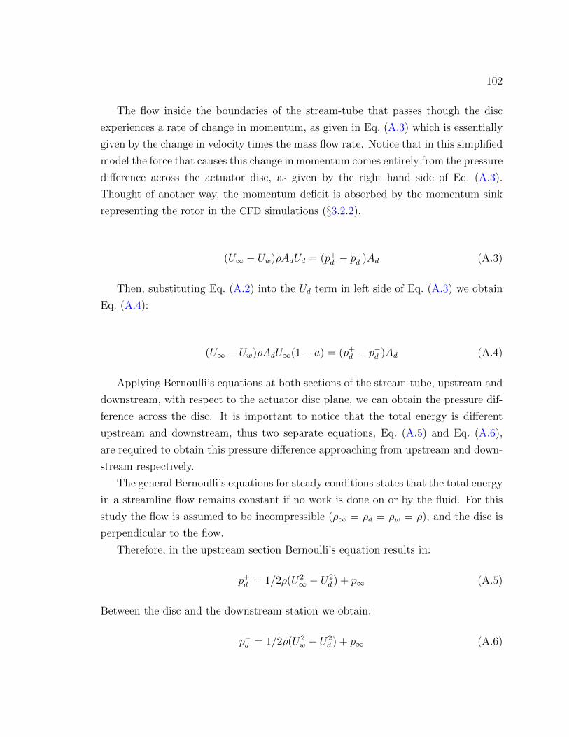
102

The flow inside the boundaries of the stream-tube that passes though the disc

experiences a rate of change in momentum, as given in Eq. (A.3) which is essentially

given by the change in velocity times the mass flow rate. Notice that in this simplified

model the force that causes this change in momentum comes entirely from the pressure

difference across the actuator disc, as given by the right hand side of Eq. (A.3).

Thought of another way, the momentum deficit is absorbed by the momentum sink

representing the rotor in the CFD simulations (§3.2.2).

(U∞ − Uw)ρAdUd = (p+d − p

−d )Ad (A.3)

Then, substituting Eq. (A.2) into the Ud term in left side of Eq. (A.3) we obtain

Eq. (A.4):

(U∞ − Uw)ρAdU∞(1− a) = (p+d − p

−d )Ad (A.4)

Applying Bernoulli’s equations at both sections of the stream-tube, upstream and

downstream, with respect to the actuator disc plane, we can obtain the pressure dif-

ference across the disc. It is important to notice that the total energy is different

upstream and downstream, thus two separate equations, Eq. (A.5) and Eq. (A.6),

are required to obtain this pressure difference approaching from upstream and down-

stream respectively.

The general Bernoulli’s equations for steady conditions states that the total energy

in a streamline flow remains constant if no work is done on or by the fluid. For this

study the flow is assumed to be incompressible (ρ∞ = ρd = ρw = ρ), and the disc is

perpendicular to the flow.

Therefore, in the upstream section Bernoulli’s equation results in:

p+d = 1/2ρ(U2

∞ − U2d ) + p∞ (A.5)

Between the disc and the downstream station we obtain:

p−d = 1/2ρ(U2w − U2

d ) + p∞ (A.6)

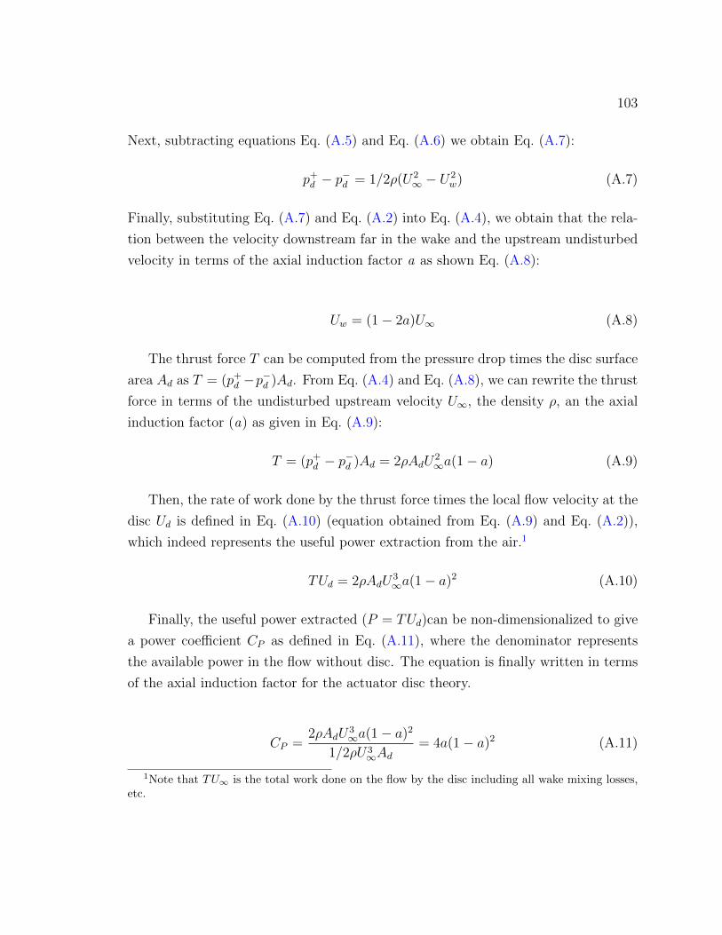
103

Next, subtracting equations Eq. (A.5) and Eq. (A.6) we obtain Eq. (A.7):

p+d − p

−d = 1/2ρ(U2

∞ − U2w) (A.7)

Finally, substituting Eq. (A.7) and Eq. (A.2) into Eq. (A.4), we obtain that the rela-

tion between the velocity downstream far in the wake and the upstream undisturbed

velocity in terms of the axial induction factor a as shown Eq. (A.8):

Uw = (1− 2a)U∞ (A.8)

The thrust force T can be computed from the pressure drop times the disc surface

area Ad as T = (p+d −p

−d )Ad. From Eq. (A.4) and Eq. (A.8), we can rewrite the thrust

force in terms of the undisturbed upstream velocity U∞, the density ρ, an the axial

induction factor (a) as given in Eq. (A.9):

T = (p+d − p

−d )Ad = 2ρAdU

2∞a(1− a) (A.9)

Then, the rate of work done by the thrust force times the local flow velocity at the

disc Ud is defined in Eq. (A.10) (equation obtained from Eq. (A.9) and Eq. (A.2)),

which indeed represents the useful power extraction from the air.1

TUd = 2ρAdU3∞a(1− a)2 (A.10)

Finally, the useful power extracted (P = TUd)can be non-dimensionalized to give

a power coefficient CP as defined in Eq. (A.11), where the denominator represents

the available power in the flow without disc. The equation is finally written in terms

of the axial induction factor for the actuator disc theory.

CP =2ρAdU

3∞a(1− a)2

1/2ρU3∞Ad

= 4a(1− a)2 (A.11)

1Note that TU∞ is the total work done on the flow by the disc including all wake mixing losses,etc.

104

In similar manner, the force on the actuator disc (thrust force) is non-dimensionalized,

and expressed in terms of the axial induction factor, to give a thrust coefficient CT :

CT = 4a(1− a) (A.12)

These quantities can also be defined using results from CFD and experimentally

determined quantities as:

CP =P

1/2ρU3∞Ad

(A.13)

CT =T

1/2ρU2∞Ad

(A.14)

The development of the analytic tunnel blockage correction models referred to

in Chapter 4 is based on this theoretical approach and its limiting assumptions. For

example, the maximum achievable value of power coefficient turns out to be 0.593, for

a = 1/3, commonly referred to as the Betz limit. Recall that the actuator disc model

considers the stream-tube to be completely surrounded by flow at constant pressure,

with no lateral mixing between the external and internal regions. In addition, if the

streamtube is expanding, there must be a net axial pressure force on the sides of the

streamtube, but this is ignored in the simple analytic actuator disc theory. As shown

in the CFD simulations for unbounded domain in §3.3.1 these assumptions are only

approximately true, and so the simple analytic theory must be treated with caution,

including instances when correction factors (e.g. for high thrust/induction cases) are

employed.

105

Appendix B

Finite Element Analysis Modelling

As described in Chapter 2, the experimental setup consists of a three-bladed rotor

attached to a main shaft which is driven by an electric motor mounted on a platform

above enclosed water tunnel. To connect the rotor to the motor (generator) a belt

carried up through a vertical support tube which connects to the main body of the

turbine. The main upright body (tube3)and the horizontal bodies (tube1 and tube2)

are made of alloy aluminum tubing. This appendix describes, step by step, the

methodology followed and required in the FEM analysis.

B.1 Geometry and Material Properties

The submerged structure of the testing rig, shown in Fig. 2.3 in Chapter 2, is mainly

made of high-strength aluminum (alloy 2024) tubes. This structure can be modelled

as three tubes of different length, diameter, and thickness, joined by rigid connections

as shown in Fig. 2.3. This scheme is a simplification of the structure that satisfied

the purposes of the FEM performed using ANSYS 11.0. The detailed dimensions of

each tube is presented in Table B.1.

The density and modulus of elasticity of the aluminum are about one third of the

respectively values of the steel. It is ductile and easily machined, which is why it

was chosen for this particular design. A Young’s modulus of 70 GPa, a density of

2700 kg and a Poisson’s modulus of 0.35 are considered as properties for this particular

structural model.

The yield strength of pure aluminum is 7 MPa to 11 MPa, while aluminum alloys

have yield strengths ranging from 200 MPa to 600 MPa. For this model a value of

106

Var

iable

sM

odel

1M

odel

2M

odel

3M

odel

4M

odel

5M

odel

6M

odel

7M

odel

8M

odel

9M

odel

10L

engt

htube

1cm

3030

3030

3030

3020

2020

Dia

met

ertube

1in

0.5

0.5

0.5

0.5

0.5

0.5

0.75

0.5

0.5

0.75

Wal

lth

icknes

stube

1in

0.05

80.

058

0.05

80.

065

0.06

50.

120.

120.

065

0.12

0.12

Len

gthtube

2cm

55

55

55

55

55

Dia

met

ertube

2in

0.75

0.75

0.75

0.75

0.75

0.75

0.75

0.75

0.75

0.75

Wal

lth

icknes

stube

2in

0.05

80.

058

0.05

80.

065

0.06

50.

120.

120.

065

0.12

0.12

Len

gthtube

3cm

2525

2525

2525

2525

2525

Dia

met

ertube

3in

0.75

0.75

0.75

0.75

0.75

11

0.75

11

Wal

lth

icknes

stube

3in

0.05

80.

120.

058

0.12

0.12

0.12

0.12

0.12

0.12

0.12

Tab

leB

.1:

Con

figu

rati

ons

ofst

udy

for

modal

anal

ysi

s

107

200 MPa is used as yield strength, typical of the 6061 aluminum available in the

machine shop.

The origin is located at key point 1. The tubes are defined in Ansys by keypoints

and lines as shown in Fig. B.1. The three tubes are connected by flanges at keypoints

2 and 3, and the rotor is located at keypoint 1.

Figure B.1: Rig structure modelling

The seven keypoints defined six line-elements on the model; the properties asso-

ciated with each type of tubing are set up on each of the six lines. A linear isotropic

model is selected for the aluminum material. For the nodal analysis the mass associ-

ated to the flanges connection at node 2, 3 and 7 is neglected, however the mass of

the rotor at the nose of the structure will be included for the modal analysis as a mass

point located in node 1. Nodes 5 and 6 are defined for support of a streamline-plate

that will avoid excessive disturbance and forces on the vertical tube. For this anal-

ysis, no forces will be applied to these two keypoints, the design of the streamlined

component is not yet defined. With respect the boundary conditions, displacement

and rotation about all axes are zero at keypoint 7, which connect the tubes-structure

with a platform located outside the water tunnel.

108

B.2 Forces Applied to the System

Referring to Fig. B.2 the tubing-structure will support the rotor located at key point

1, and then the force exerted by the fluid flow at the rotating set of blades will be

directly transmitted to the tubing structure. When the rotor is aligned with the

horizontal tubing and the plane of the rotor faces the flow orthogonally, the force

at node 1 is a vector acting along in the X direction only: FX as shown scheme.

The system will also operate in yawed conditions in the XZ plane. Only the plane

of the rotor is modified, and then the tubing structure keeps it location. The force

applied on node 1 will be a vector with components acting in the X and Z axis. No

yaw is exerted in the YZ plane. Forces applied on any other node are neglected in

this model. For the static analysis, the maximum possible value of these forces it is

applied.

Figure B.2: Rig structure modelling

The resultant maximum forces are summarized in Table 2.2.

Since the forces are both aligned on the rotor axis and yawed in the plane XZ,

displacement in X, Y, and Z direction can occur. A three dimensional analysis was

109

performed, and thus an element with 3D capabilities (axial, torsion and bending in

X,Y and Z directions) was used to model the tubes. In addition, a mass element was

chosen to represent the rotor attached to the horizontal tubing 1.

PIPE16 Element was selected for the tubes. PIPE16 is a uniaxial element with

tension-compression, torsion, and bending capabilities. The element has six degrees

of freedom at two nodes: translations in the nodal x, y, and z directions and ro-

tations about the nodal x, y, and z axes. This element is based on the 3-D beam

element (BEAM4), and includes simplifications due to its symmetry and standard

pipe geometry [28].

For the element input data, it was required to include the pipe outer diameter

and wall thickness, as detailed in Table B.1. The density of the material, elasticity

and Poison’s ratio was already defined in material properties for aluminum material.

The element mass is calculated from the pipe wall material.

To represent the mass associated with the rotor, the MASS21 element is available

in ANSYS. MASS21 is a point element having up to six degrees of freedom: displace-

ment in the X, Y and Z direction and rotation about the nodal X, Y and Z axes. The

mass element is defined by a single node; in this case associated to keypoint 1, and

having a mass of 30 gr.

B.3 Maximum Deflection - Results

The maximum deflection and stresses were computed for the forces estimated at the

rotor plane for both, the yawed and non-yawed condition (see Table 2.2 in Chapter 2.

The following Table B.2 shows the maximum deflections and the maximum stresses

(von Misses) computed when the inflow is aligned with the axis of the turbine.

Observing the system loaded in the axial turbine direction only, which is the stiffer

condition of the structure, models 1 to 4 already experienced deflections of 1 mm or

larger. Consequently, those first four configuration were no longer considered for the

yawed condition analysis. Tables B.3 and B.5 present the maximum deflection of the

structure and maximum von Mises stresses computed for the yawed conditions of 30

and 45 respectively.

110

Case Max.deflections [mm] Max.Stress [MPa]Model1 1.63 24Model2 0.997 14.7Model3 7.31 68.40Model4 0.997 14.7Model5 0.374 7.31Model6 0.374 7.31Model7 0.374 7.31Model8 0.764 14.7Model9 0.286 7.31Model10 0.286 7.31

Table B.2: Maximum deflections and stresses (Non-yawed condition)

Case Max.deflections [mm] Max.Stress [MPa]Model5 1.5 6.91Model6 1.228 6.91Model7 0.645 6.91Model8 1.064 13.5Model9 0.506 6.57Model10 0.358 6.57

Table B.3: Max.deflections and stresses at 30 yaw angle

B.4 Modal Analysis - Results

Results of the modal analysis for models 5 to 10 are presented in Table B.5:

B.5 Mesh Refinement

The structure was defined by 7 keypoints; six element lines Pipe 16 and one element

MASS 21 at node and keypoint 1. Different elements size were computed to study

the effect of the number of elements in results of the model.

In general terms, a fine mesh allows the definition of small ”sub elements” to get

good values of the distribution of stresses along the total length of each element. In

such a way the solution and stress values will be more precise, and it is possible to

111

Case Max.deflections [mm] Max.Stress [MPa]Model5 2.155 4Model6 1.736 3.84Model7 0.817 3.84Model8 1.219 6.69Model9 0.646 3.37Model10 0.378 3.37

Table B.4: Maximum deflections and stresses at 45 yaw angle

Mode Model5 Model6 Model7 Model8 Model9 Model10

Mode1 55 56 69 74 97 108Mode2 576 59 76 82 105 117Mode3 204 184 196 175 217 260Mode4 263 235 237 215 274 289Mode5 543 506 713 897 947 1, 292Mode6 555 523 742 951 1, 002 1, 293Mode7 1, 446 1, 333 1, 627 1, 385 1, 684 1, 818Mode8 1, 466 1, 374 1, 635 1, 407 1, 774 1, 874Mode9 1, 785 1, 743 2, 087 2, 650 2, 549 3, 360Mode10 1, 885 1, 797 2, 204 3, 014 3, 031 3, 677

Table B.5: Result of modal analysis - natural frequencies [Hz]

identify areas with higher critical tensile stresses in the structure. Specially, when

there are distributed loads applied to the system, and the purpose of the analysis is

to resolve peak bending stresses, the node point should be near the real location of

the peak value, otherwise the linear bending moment can be underestimated. In this

particular model there is only one point load. Even if the maximum displacement

obtained will be not affected by the mesh size, since a modal analysis was also per-

formed, it was important to obtain accurate solutions for the peak stresses, so mesh

refinement was performed.

Note that the maximum number of nodes that the Academic Version of Ansys

11.0 allows is 32, 000. Thus, the smallest possible element for this model has a length

of 0.025 mm.

112

For the mesh analysis, a modal analysis was performed over the Model10 config-

uration, with the mass element added at key point 1, considering different element

sizes for the mesh. The first 20 modes of each coarser mesh of element sizes 100 mm,

10 mm, 1 mm, and 0.1 m were compared to the modes obtained for the finest possible

mesh of element size 0.025 mm.

Figure B.2 show the differences between the frequency results obtained for each

coarser (100 mm, 10 mm, 1 mm, and 0.1 mm) mesh and the finest possible mesh

allowed by software limitations. It was found that an element of 0.1 mm size provides

accurate enough results compared against to the results obtained for the finest mesh.

Thus, this 0.1 mm element size is used to compute the static and modal analysis for

the different set of configurations.

-25.00%

-20.00%

-15.00%

-10.00%

-5.00%

0.00%

5.00%

0 5 10 15 20 25

Modes

Mesh_100_mm

Dif

fere

nc

e (%

)

-0.25%

-0.20%

-0.15%

-0.10%

-0.05%

0.00%

0.05%

0 5 10 15 20 25

Modes

Mesh_10_mm

Dif

fere

nc

e (%

)

-0.003%

-0.003%

-0.002%

-0.002%

-0.001%

-0.001%

0.000%

0.001%

0 5 10 15 20 25

Modes

Mesh_1_mmD

iffe

ren

ce

(%

)

0.000%

0.020%

0.040%

0.060%

0.080%

0.100%

0 5 10 15 20 25

Modes

Mesh_0.1_mm

Dif

fere

nc

e (%

)

Figure B.3: Mesh analysis (Model10)

113

Appendix C

PIV Theory

The fundamental premise of the PIV technique is that instantaneous fluid velocities

can be evaluated by recording the position of images produced by small markers,

suspended in the fluid, at consecutive intervals time. This concept assumes that the

small particles follow the fluid motion, with minimal lag, and do not modify the fluid

properties. Solid particles are often employed as markers, either in liquid or gas fluid

flow.

In a typical arrangement of a PIV system, the fluid being studied is illuminated

by a pulsed light sheet. A photograph or video device is located in the plane perpen-

dicular to the sheet to capture the light reflected by the particles seeded in the fluid

that follow the flow motion. Finally, the information is transferred to a computer to

be analyzed [53].

By controlling the pulse light and the continuity of the image recording (frame)

several representations of pulse code and framing can be obtained, for example multi-

frame/single-pulse, etc. The relevance of the pulse code is to provide images of

the location of the particles in an interval of time ∆t that allows calculating the

displacement of the particles for a particular flow condition. The separation of the

pulses ∆t of light in addition to light intensity are the factors that rule the range of

velocity possible to be measured, and the sharpness of the particle picture obtained

[53].

Two distinct operation modes are possible in this technique: the autocorrela-

tion mode where two or more instantaneous image patters created by the tracers is

recorded in the same frame; and the cross-correlation mode, in which the individual

instantaneous patterns are kept in separate frames. The time separation between

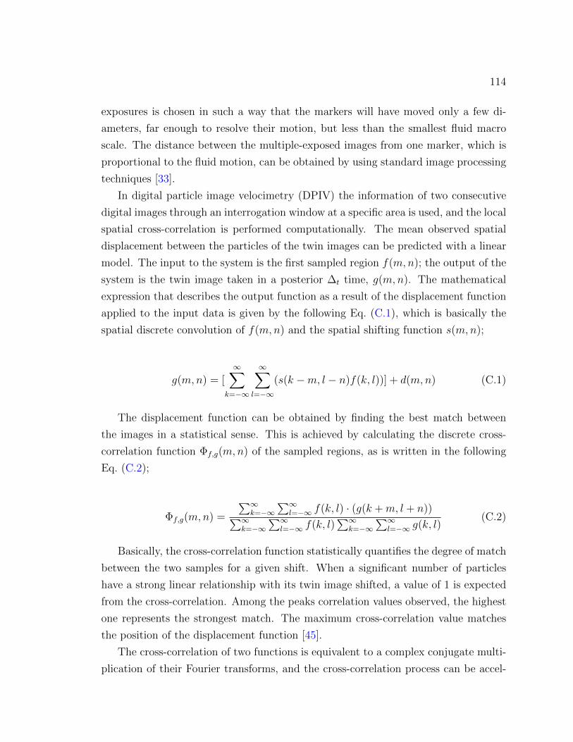
114

exposures is chosen in such a way that the markers will have moved only a few di-

ameters, far enough to resolve their motion, but less than the smallest fluid macro

scale. The distance between the multiple-exposed images from one marker, which is

proportional to the fluid motion, can be obtained by using standard image processing

techniques [33].

In digital particle image velocimetry (DPIV) the information of two consecutive

digital images through an interrogation window at a specific area is used, and the local

spatial cross-correlation is performed computationally. The mean observed spatial

displacement between the particles of the twin images can be predicted with a linear

model. The input to the system is the first sampled region f(m,n); the output of the

system is the twin image taken in a posterior ∆t time, g(m,n). The mathematical

expression that describes the output function as a result of the displacement function

applied to the input data is given by the following Eq. (C.1), which is basically the

spatial discrete convolution of f(m,n) and the spatial shifting function s(m,n);

g(m,n) = [∞∑

k=−∞

∞∑l=−∞

(s(k −m, l − n)f(k, l))] + d(m,n) (C.1)

The displacement function can be obtained by finding the best match between

the images in a statistical sense. This is achieved by calculating the discrete cross-

correlation function Φf,g(m,n) of the sampled regions, as is written in the following

Eq. (C.2);

Φf,g(m,n) =

∑∞k=−∞

∑∞l=−∞ f(k, l) · (g(k +m, l + n))∑∞

k=−∞∑∞

l=−∞ f(k, l)∑∞

k=−∞∑∞

l=−∞ g(k, l)(C.2)

Basically, the cross-correlation function statistically quantifies the degree of match

between the two samples for a given shift. When a significant number of particles

have a strong linear relationship with its twin image shifted, a value of 1 is expected

from the cross-correlation. Among the peaks correlation values observed, the highest

one represents the strongest match. The maximum cross-correlation value matches

the position of the displacement function [45].

The cross-correlation of two functions is equivalent to a complex conjugate multi-

plication of their Fourier transforms, and the cross-correlation process can be accel-

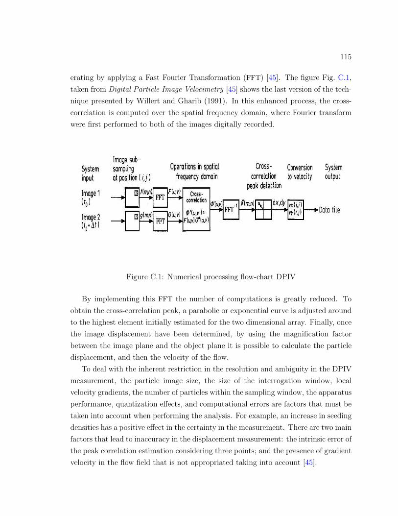
115

erating by applying a Fast Fourier Transformation (FFT) [45]. The figure Fig. C.1,

taken from Digital Particle Image Velocimetry [45] shows the last version of the tech-

nique presented by Willert and Gharib (1991). In this enhanced process, the cross-

correlation is computed over the spatial frequency domain, where Fourier transform

were first performed to both of the images digitally recorded.

Figure C.1: Numerical processing flow-chart DPIV

By implementing this FFT the number of computations is greatly reduced. To

obtain the cross-correlation peak, a parabolic or exponential curve is adjusted around

to the highest element initially estimated for the two dimensional array. Finally, once

the image displacement have been determined, by using the magnification factor

between the image plane and the object plane it is possible to calculate the particle

displacement, and then the velocity of the flow.

To deal with the inherent restriction in the resolution and ambiguity in the DPIV

measurement, the particle image size, the size of the interrogation window, local

velocity gradients, the number of particles within the sampling window, the apparatus

performance, quantization effects, and computational errors are factors that must be

taken into account when performing the analysis. For example, an increase in seeding

densities has a positive effect in the certainty in the measurement. There are two main

factors that lead to inaccuracy in the displacement measurement: the intrinsic error of

the peak correlation estimation considering three points; and the presence of gradient

velocity in the flow field that is not appropriated taking into account [45].

116

In the experiment carried out by Willert and Gharib [45], which studied the tem-

poral evolution of a vortex ring, the displacement vector obtained shows areas of high

velocity gradients near the center of the core. These gradients will bias the cross-

correlation peak. To avoid this effect, a possible solution is to lessen the sampling

window for the analysis, but this action will also affect the spatial resolution because

the lower density seeding of the images taken [2]. Then, the way to deal with this

problem is to remove the doubtful data which could lead to misinterpretation, and

some vectors for each data set must be interpolated with the associated loss of infor-

mation. Also, a convolution filtering (low pass spatial filter) could be applied to the

data, which eliminates the high frequency jitter associated with the different location

estimates of the cross-correlation peak, with no information lost. The validation of

the measurements is so far the most difficult and laborious duty within this whole

process [45].

Several types of errors can be found in velocity measurement in DPIV; however,

the interesting point is the errors in the particle displacement calculation. This er-

ror can be the result of not choosing the most appropriate method to extract the

displacement peak from the correlation function, or for distortion of the correlation

function, for example due to velocity gradient [48]. Fortily and Strykowsky (2000)

presented a procedure that allows quantifying the bias and precision errors of DPIV

in an attempt to correct the systematic error presented in the mean displacement

measurements.

In this procedure [48], to resolve the directional ambiguity two digital images at

each pulse separation were taken within this region a wide range of flow gradients are

presented, and the digital images are processing with the different algorithms available

in the software package that is being utilized for the experiment. Firstly, images must

be taken for non-flow conditions, several uniform displacement images are generated

by varying the mirror speed and pulse separation, in this fashion a wide range of

displacement and a detailed measurement of the sub-pixel displacement region are

obtained. For example, if the sampling windows size has 128x128 pixels, and the

images are interrogated on a spatial grid of 30x10 displacement measurements over the

image domain, then 300 displacement vectors can be obtained for each image. If the

interrogation windows are large, the displacement peaks results clearly taller than the

noise peaks, at each image. Finally, the bias error can be calculated as the difference

between the displacement measured and the displacement generated (at each pulse

117

separation), which represents the error in the average displacement measured. This

calibration process is suggested to find the best mathematical algorithm option, for

the particular experimental set up, within the available methods available in the

software in use.