development document for the final revisions to the national

Development Document for the Final Revisions to the National PollutantDischarge Elimination System Regulationand the Effluent Guidelines forConcentrated Animal Feeding Operations

December 2002

U.S. Environmental Protection AgencyOffice of Water (4303T)

1200 Pennsylvania Avenue, NWWashington, DC 20460

EPA-821-R-03-001

Development Document for the Final Revisions to the National

Pollutant Discharge Elimination System Regulation and the

Effluent Guidelines for

Concentrated Animal Feeding Operations

Christine Todd WhitmanAdministrator

Tracey Mehan. IIIAssistant Administrator, Office of Water

Sheila E. FraceDirector, Engineering and Analysis Division

Donald F. AndersonChief, Commodities Branch

Paul H. ShrinerProject Manager

Ronald JordanTechnical Coordinator

Engineering and Analysis DivisionOffice of Science and Technology

U.S. Environmental Protection AgencyWashington, D.C. 20460

December 2002

ii

ACKNOWLEDGMENTS AND DISCLAIMER

This report has been reviewed and approved for publication by the Engineeringand Analysis Division, Office of Science and Technology. This report wasprepared with the support of Tetra Tech, Inc., and Eastern Research Group, Inc.,under the direction and review of the Office of Science and Technology.

Neither the United States government nor any of its employees, contractors,subcontractors, or other employees makes any warranty, expressed or implied, orassumes any legal liability or responsibility for any third party’s use of, or theresults of such use of, any information, apparatus, product, or process discussed inthis report, or represents that its use by such a third party would not infringe onprivately owned rights.

iii

CONTENTS

Chapter 1 Introduction and Legal Authority . . . . . . . . . . . . . . . . . . . . . . . . . . . . . . . . . . . . . . . 1-1

1.0 INTRODUCTION AND LEGAL AUTHORITY . . . . . . . . . . . . . . . . . . . . . . . . . . . . . . . . . . . . 1-1

1.1 Clean Water Act (CWA) . . . . . . . . . . . . . . . . . . . . . . . . . . . . . . . . . . . . . . . . . 1-1

1.1.1 National Pollutant Discharge Elimination System . . . . . . . . . . . . . . . 1-2

1.1.2 Effluent Limitations Guidelines and Standards . . . . . . . . . . . . . . . . . . 1-2

1.2 Pollution Prevention Act . . . . . . . . . . . . . . . . . . . . . . . . . . . . . . . . . . . . . . . . . . 1-5

1.3 Regulatory Flexibility Act as Amended by the Small Business RegulatoryEnforcement Fairness Act of 1996 (SBREFA) . . . . . . . . . . . . . . . . . . . . . . . . 1-5

Chapter 2 Summary and Scope of Final Regulation . . . . . . . . . . . . . . . . . . . . . . . . . . . . . . . . . 2-1

2.0 SUMMARY AND SCOPE OF FINAL REGULATION . . . . . . . . . . . . . . . . . . . . . . . . . . . . . . . 2-1

2.1 National Pollutant Discharge Elimination System . . . . . . . . . . . . . . . . . . . . . . 2-1

2.1.1 Applicability of the Final Regulation . . . . . . . . . . . . . . . . . . . . . . . . . 2-1

2.1.2 Summary of Revisions to NPDES Regulations . . . . . . . . . . . . . . . . . . 2-3

2.2 Effluent Limitations Guidelines and Standards . . . . . . . . . . . . . . . . . . . . . . . . 2-5

2.2.1 Applicability of the Final Regulation . . . . . . . . . . . . . . . . . . . . . . . . . 2-6

2.2.2 Summary of Revisions to Effluent Limitations Guidelines and Standards . . . . . . . . . . . . . . . . . . . . . . . . . . . . . . . . . . . . . . . . . . . . 2-9

2.2.2.1 Land Application Best Practicable Control Technology . . . . . . . . . . . . . . . . . . . . . . . . . . . . . . . . . . . . 2-9

2.2.2.2 Production Area Best Practicable Control Technology . . . . . . . . . . . . . . . . . . . . . . . . . . . . . . . . . . . 2-11

2.2.2.3 Best Control Technology . . . . . . . . . . . . . . . . . . . . . . . . 2-12

2.2.2.4 Best Available Technology . . . . . . . . . . . . . . . . . . . . . . 2-12

2.2.2.5 New Source Performance Standards . . . . . . . . . . . . . . . 2-12

2.2.2.6 Voluntary Alternative Performance Standards to Encourage Innovative Technologies . . . . . . . . . . . . . 2-15

2.2.2.7 Voluntary Superior EnvironmentalPerformance Standards for New Large Swine/Poultry/Veal CAFOs . 2-16

Chapter 3 Data Collection Activities . . . . . . . . . . . . . . . . . . . . . . . . . . . . . . . . . . . . . . . . . . . . . . 3-1

3.0 DATA COLLECTION ACTIVITIES . . . . . . . . . . . . . . . . . . . . . . . . . . . . . . . . . . . . . . . . . . . 3-1

3.1 Summary of EPA’s Site Visit Program . . . . . . . . . . . . . . . . . . . . . . . . . . . . . . 3-2

3.2 Industry Trade Associations . . . . . . . . . . . . . . . . . . . . . . . . . . . . . . . . . . . . . . . 3-4

3.3 U.S. Department of Agriculture . . . . . . . . . . . . . . . . . . . . . . . . . . . . . . . . . . . . 3-5

3.3.1 National Agricultural Statistics Service . . . . . . . . . . . . . . . . . . . . . . . 3-6

iv

3.3.2 Animal and Plant Health Inspection Service National Animal HealthMonitoring System (NAHMS) . . . . . . . . . . . . . . . . . . . . . . . . . . . . . . 3-8

3.3.3 Natural Resources Conservation Services . . . . . . . . . . . . . . . . . . . . . 3-10

3.3.4 Agricultural Research Service (ARS) . . . . . . . . . . . . . . . . . . . . . . . . 3-11

3.3.5 Economic Research Service (ERS) . . . . . . . . . . . . . . . . . . . . . . . . . . 3-11

3.4 Other Agency Reports . . . . . . . . . . . . . . . . . . . . . . . . . . . . . . . . . . . . . . . . . . 3-12

3.5 Literature Sources . . . . . . . . . . . . . . . . . . . . . . . . . . . . . . . . . . . . . . . . . . . . . . 3-12

3.6 References . . . . . . . . . . . . . . . . . . . . . . . . . . . . . . . . . . . . . . . . . . . . . . . . . . . . 3-12

Chapter 4 Industry Profiles . . . . . . . . . . . . . . . . . . . . . . . . . . . . . . . . . . . . . . . . . . . . . . . . . . . . . 4-1

4.0 INTRODUCTION . . . . . . . . . . . . . . . . . . . . . . . . . . . . . . . . . . . . . . . . . . . . . . . . . . . . . . . . 4-1

4.1 Swine Industry Description . . . . . . . . . . . . . . . . . . . . . . . . . . . . . . . . . . . . . . . 4-1

4.1.1 Distribution of Swine Operations by Size and Region . . . . . . . . . . . . 4-3

4.1.1.1 National Overview . . . . . . . . . . . . . . . . . . . . . . . . . . . . . . 4-4

4.1.1.2 Operations by Size Class . . . . . . . . . . . . . . . . . . . . . . . . . 4-4

4.1.1.3 Regional Variation in Hog Operations . . . . . . . . . . . . . . . 4-5

4.1.2 Production Cycles of Swine . . . . . . . . . . . . . . . . . . . . . . . . . . . . . . . . 4-9

4.1.3 Swine Facility Types and Management . . . . . . . . . . . . . . . . . . . . . . . 4-12

4.1.4 Swine Waste Management Practices . . . . . . . . . . . . . . . . . . . . . . . . . 4-16

4.1.4.1 Swine Waste Collection Practices . . . . . . . . . . . . . . . . . 4-17

4.1.4.2 Swine Waste Storage Practices . . . . . . . . . . . . . . . . . . . 4-17

4.1.4.3 Swine Waste Treatment Practices . . . . . . . . . . . . . . . . . 4-20

4.1.4.4 Waste Management Practices by Operation Size andGeographical Location . . . . . . . . . . . . . . . . . . . . . . . . . . 4-22

4.1.5 Pollution Reduction . . . . . . . . . . . . . . . . . . . . . . . . . . . . . . . . . . . . . 4-28

4.1.5.1 Swine Feeding Strategies . . . . . . . . . . . . . . . . . . . . . . . . 4-28

4.1.5.2 Waste and Waste Water Reductions . . . . . . . . . . . . . . . 4-31

4.1.6 Waste Disposal . . . . . . . . . . . . . . . . . . . . . . . . . . . . . . . . . . . . . . . . . 4-32

4.2 Poultry Industry . . . . . . . . . . . . . . . . . . . . . . . . . . . . . . . . . . . . . . . . . . . . . . . 4-35

4.2.1 Broiler Sector . . . . . . . . . . . . . . . . . . . . . . . . . . . . . . . . . . . . . . . . . . . 4-36

4.2.1.1 Distribution of Broiler Operations by Size and Region 4-37

4.2.1.2 Production Cycles of Broilers . . . . . . . . . . . . . . . . . . . . 4-40

4.2.1.3 Broiler Facility Types and Management . . . . . . . . . . . . 4-41

4.2.1.4 Broiler Waste Management Practices . . . . . . . . . . . . . . 4-42

4.2.1.5 Pollution Reduction . . . . . . . . . . . . . . . . . . . . . . . . . . . . 4-43

4.2.1.6 Waste Disposal . . . . . . . . . . . . . . . . . . . . . . . . . . . . . . . . 4-44

4.2.2 Layer Sector . . . . . . . . . . . . . . . . . . . . . . . . . . . . . . . . . . . . . . . . . . . . 4-45

4.2.2.1 Distribution of Layer Operations by Size and Region . 4-46

4.2.2.2 Production Cycles of Layers and Pullets . . . . . . . . . . . . 4-49

4.2.2.3 Layer Facility Types and Management . . . . . . . . . . . . . 4-49

v

4.2.2.4 Layer Waste Management Practices . . . . . . . . . . . . . . . 4-51

4.2.2.5 Layer Egg Wash Water . . . . . . . . . . . . . . . . . . . . . . . . . 4-51

4.2.2.6 Waste and Wastewater Reductions . . . . . . . . . . . . . . . . 4-53

4.2.2.7 Waste Disposal . . . . . . . . . . . . . . . . . . . . . . . . . . . . . . . . 4-53

4.2.3 Turkey Sector . . . . . . . . . . . . . . . . . . . . . . . . . . . . . . . . . . . . . . . . . . . 4-55

4.2.3.1 Distribution of Turkey Operations by Size and Region 4-56

4.2.3.2 Production Cycles of Turkeys . . . . . . . . . . . . . . . . . . . . 4-58

4.2.3.3 Turkey Facility Types and Management . . . . . . . . . . . . 4-58

4.2.3.4 Turkey Waste Management Practices . . . . . . . . . . . . . . 4-59

4.2.3.5 Pollution Reduction . . . . . . . . . . . . . . . . . . . . . . . . . . . . 4-60

4.2.3.6 Waste Disposal . . . . . . . . . . . . . . . . . . . . . . . . . . . . . . . . 4-60

4.2.4 Duck Sector . . . . . . . . . . . . . . . . . . . . . . . . . . . . . . . . . . . . . . . . . . . . 4-61

4.2.4.1 Distribution of the Duck Industry by Size and Region . 4-61

4.3 Dairy Industry . . . . . . . . . . . . . . . . . . . . . . . . . . . . . . . . . . . . . . . . . . . . . . . . . 4-62

4.3.1 Distribution of Dairy Operations by Size and Region . . . . . . . . . . . . 4-62

4.3.2 Dairy Production Cycles . . . . . . . . . . . . . . . . . . . . . . . . . . . . . . . . . . 4-65

4.3.2.1 Milk Herd . . . . . . . . . . . . . . . . . . . . . . . . . . . . . . . . . . . . 4-66

4.3.2.2 Calves, Heifers, and Bulls . . . . . . . . . . . . . . . . . . . . . . . 4-66

4.3.3 Stand-Alone Heifer Raising Operations . . . . . . . . . . . . . . . . . . . . . . 4-67

4.3.4 Dairy Facility Management . . . . . . . . . . . . . . . . . . . . . . . . . . . . . . . . 4-69

4.3.4.1 Housing Practices . . . . . . . . . . . . . . . . . . . . . . . . . . . . . . 4-69

4.3.4.2 Flooring and Bedding . . . . . . . . . . . . . . . . . . . . . . . . . . . 4-73

4.3.4.3 Feeding and Watering Practices . . . . . . . . . . . . . . . . . . . 4-74

4.3.4.4 Milking Operations . . . . . . . . . . . . . . . . . . . . . . . . . . . . 4-75

4.3.4.5 Rotational Grazing . . . . . . . . . . . . . . . . . . . . . . . . . . . . . 4-77

4.3.5 Dairy Waste Management Practices . . . . . . . . . . . . . . . . . . . . . . . . . 4-80

4.3.5.1 Waste Collection . . . . . . . . . . . . . . . . . . . . . . . . . . . . . . 4-81

4.3.5.2 Transport . . . . . . . . . . . . . . . . . . . . . . . . . . . . . . . . . . . . 4-82

4.3.5.3 Storage, Treatment, and Disposal . . . . . . . . . . . . . . . . . 4-82

4.4 Beef Industry . . . . . . . . . . . . . . . . . . . . . . . . . . . . . . . . . . . . . . . . . . . . . . . . . . 4-83

4.4.1 Distribution of the Beef Industry by Size and Region . . . . . . . . . . . . 4-84

4.4.2 Beef Production Cycles . . . . . . . . . . . . . . . . . . . . . . . . . . . . . . . . . . . 4-87

4.4.3 Beef Feedlot Facility Management . . . . . . . . . . . . . . . . . . . . . . . . . . 4-88

4.4.3.1 Feedlot Systems . . . . . . . . . . . . . . . . . . . . . . . . . . . . . . . 4-88

4.4.3.2 Feeding and Watering Practices . . . . . . . . . . . . . . . . . . . 4-89

4.4.3.3 Water Use and Wastewater Generation . . . . . . . . . . . . . 4-90

4.4.3.4 Climate . . . . . . . . . . . . . . . . . . . . . . . . . . . . . . . . . . . . . . 4-91

4.4.4 Backgrounding Operations . . . . . . . . . . . . . . . . . . . . . . . . . . . . . . . . 4-91

4.4.5 Veal Operations . . . . . . . . . . . . . . . . . . . . . . . . . . . . . . . . . . . . . . . . . 4-91

4.4.6 Cow-Calf Operations . . . . . . . . . . . . . . . . . . . . . . . . . . . . . . . . . . . . . 4-92

vi

4.4.7 Waste Management Practices . . . . . . . . . . . . . . . . . . . . . . . . . . . . . . 4-93

4.4.7.1 Waste Collection . . . . . . . . . . . . . . . . . . . . . . . . . . . . . . 4-93

4.4.7.2 Transport . . . . . . . . . . . . . . . . . . . . . . . . . . . . . . . . . . . . 4-94

4.4.7.3 Storage, Treatment, and Disposal . . . . . . . . . . . . . . . . . 4-95

4.5 Horses . . . . . . . . . . . . . . . . . . . . . . . . . . . . . . . . . . . . . . . . . . . . . . . . . . . . . . . 4-96

4.5.1 Distribution of the Horse Industry by Size and Region . . . . . . . . . . . 4-96

4.5.2 Waste Management Practices . . . . . . . . . . . . . . . . . . . . . . . . . . . . . . 4-98

4.5.2.1 Waste Storage . . . . . . . . . . . . . . . . . . . . . . . . . . . . . . . . 4-99

4.5.2.2 Waste Treatment and Disposal . . . . . . . . . . . . . . . . . . 4-100

4.6 References . . . . . . . . . . . . . . . . . . . . . . . . . . . . . . . . . . . . . . . . . . . . . . . . . . . 4-101

Chapter 5 Industry Subcategorization for Effluent Limitations Guidelines and Standards . 5-1

5.0 INTRODUCTION . . . . . . . . . . . . . . . . . . . . . . . . . . . . . . . . . . . . . . . . . . . . . . . . . . . . . . . . 5-1

5.1 Background . . . . . . . . . . . . . . . . . . . . . . . . . . . . . . . . . . . . . . . . . . . . . . . . . . . . 5-2

5.2 Subcategorization Basis for the Final Rule . . . . . . . . . . . . . . . . . . . . . . . . . . . 5-3

5.2.1 Animal Production, Manure Management, and Waste HandlingProcesses . . . . . . . . . . . . . . . . . . . . . . . . . . . . . . . . . . . . . . . . . . . . . . . 5-3

5.2.2 Other factors . . . . . . . . . . . . . . . . . . . . . . . . . . . . . . . . . . . . . . . . . . . . 5-7

Chapter 6 Wastewater Characterization and Manure Characteristics . . . . . . . . . . . . . . . . . . 6-1

6.0 INTRODUCTION . . . . . . . . . . . . . . . . . . . . . . . . . . . . . . . . . . . . . . . . . . . . . . . . . . . . . . . . 6-1

6.1 Swine Waste . . . . . . . . . . . . . . . . . . . . . . . . . . . . . . . . . . . . . . . . . . . . . . . . . . . 6-1

6.1.1 Quantity of Manure Generated . . . . . . . . . . . . . . . . . . . . . . . . . . . . . . 6-3

6.1.2 Description of Waste Constituents and Concentrations . . . . . . . . . . . 6-4

6.2 Poultry Waste . . . . . . . . . . . . . . . . . . . . . . . . . . . . . . . . . . . . . . . . . . . . . . . . . 6-10

6.2.1 Broiler Waste Characteristics . . . . . . . . . . . . . . . . . . . . . . . . . . . . . . 6-11

6.2.1.1 Quantity of Manure Generated . . . . . . . . . . . . . . . . . . . 6-11

6.2.1.2 Description of Waste Constituents and Concentrations . . . . . . . . . . . . . . . . . . . . . . . . . . . . . . . . 6-11

6.2.2 Layer Waste Characteristics . . . . . . . . . . . . . . . . . . . . . . . . . . . . . . . 6-13

6.2.2.1 Quantity of Manure Generated . . . . . . . . . . . . . . . . . . . . . . . 6-13

6.2.2.2 Description of Waste Constituents and Concentrations . . . . . . . . . . . . . . . . . . . . . . . . . . . . . . . . . . . . . . . . . . . . 6-14

6.2.3 Turkey Waste Characteristics . . . . . . . . . . . . . . . . . . . . . . . . . . . . . . 6-17


6.2.3.2 Description of Waste Constituents and Concentrations . . . . . . . . . . . . . . . . . . . . . . . . . . . . . . . . 6-17

6.2.4 Duck Wastes . . . . . . . . . . . . . . . . . . . . . . . . . . . . . . . . . . . . . . . . . . . 6-21


6.2.4.2 Description of Waste Constituents and Concentrations 6-22

vii

6.3 Dairy Waste . . . . . . . . . . . . . . . . . . . . . . . . . . . . . . . . . . . . . . . . . . . . . . . . . . 6-22

6.3.1 Quantity of Manure Generated . . . . . . . . . . . . . . . . . . . . . . . . . . . . . 6-22

6.3.2 Waste Constituents and Concentrations . . . . . . . . . . . . . . . . . . . . . . 6-23

6.3.2.1 Composition of Fresh Manure . . . . . . . . . . . . . . . . . . . . 6-23

6.3.2.2 Composition of Stored or Managed Waste . . . . . . . . . . 6-25

6.3.2.3 Composition of Aged Manure/Waste . . . . . . . . . . . . . . . 6-27

6.4 Beef and Heifer Waste . . . . . . . . . . . . . . . . . . . . . . . . . . . . . . . . . . . . . . . . . . 6-28



6.4.2.1 Composition of “As-Excreted” Manure . . . . . . . . . . . . . 6-29

6.4.2.2 Composition of Beef and Heifer Feedlot Waste . . . . . . 6-31

6.4.2.3 Composition of Aged Manure . . . . . . . . . . . . . . . . . . . . 6-33

6.4.2.4 Composition of Runoff from Beef and Heifer Feedlots . . . . . . . . . . . . . . . . . . . . . . . . . . . . . . . 6-33

6.5 Veal Waste . . . . . . . . . . . . . . . . . . . . . . . . . . . . . . . . . . . . . . . . . . . . . . . . . . . 6-34



6.6 Horse Waste . . . . . . . . . . . . . . . . . . . . . . . . . . . . . . . . . . . . . . . . . . . . . . . . . . 6-36


6.6.2 Horse Waste Characteristics . . . . . . . . . . . . . . . . . . . . . . . . . . . . . . . 6-37

6.7 References . . . . . . . . . . . . . . . . . . . . . . . . . . . . . . . . . . . . . . . . . . . . . . . . . . . . 6-37

Chapter 7 Pollutants of Interest . . . . . . . . . . . . . . . . . . . . . . . . . . . . . . . . . . . . . . . . . . . . . . . . . . 7-1

7.0 INTRODUCTION . . . . . . . . . . . . . . . . . . . . . . . . . . . . . . . . . . . . . . . . . . . . . . . . . . . . . . . . 7-1

7.1 Conventional Waste Pollutants . . . . . . . . . . . . . . . . . . . . . . . . . . . . . . . . . . . . . 7-2

7.2 Nonconventional Pollutants . . . . . . . . . . . . . . . . . . . . . . . . . . . . . . . . . . . . . . . 7-3

7.3 Priority Pollutants . . . . . . . . . . . . . . . . . . . . . . . . . . . . . . . . . . . . . . . . . . . . . . 7-11

7.4 References . . . . . . . . . . . . . . . . . . . . . . . . . . . . . . . . . . . . . . . . . . . . . . . . . . . . 7-12

Chapter 8 Treatment Technologies and Best Management Practices . . . . . . . . . . . . . . . . . . . 8-18.0 INTRODUCTION . . . . . . . . . . . . . . . . . . . . . . . . . . . . . . . . . . . . . . . . . . . . . . . . . . . . . . . . 8-1

8.1 Pollution Prevention Practices . . . . . . . . . . . . . . . . . . . . . . . . . . . . . . . . . . . . . 8-1

8.1.1 Feeding Strategies . . . . . . . . . . . . . . . . . . . . . . . . . . . . . . . . . . . . . . . . 8-1

8.1.1.1 Swine Feeding Strategies . . . . . . . . . . . . . . . . . . . . . . . . . 8-2

8.1.1.2 Poultry Feeding Strategies . . . . . . . . . . . . . . . . . . . . . . . . 8-6

8.1.1.3 Dairy Feeding Strategies . . . . . . . . . . . . . . . . . . . . . . . . . 8-9

8.1.2 Reduced Water Use and Water Content of Waste . . . . . . . . . . . . . . . 8-15

8.2 Manure/Waste Handling Storage and Treatment Technologies . . . . . . . . . . . 8-44

8.2.1 Waste Handling Technologies and Practices . . . . . . . . . . . . . . . . . . . 8-44

8.2.2 Waste Storage Technologies and Practices . . . . . . . . . . . . . . . . . . . . 8-51

viii

8.2.3 Waste Treatment Technologies and Practices . . . . . . . . . . . . . . . . . . 8-67

8.2.3.1 Treatment of Animal Wastes and Wastewater . . . . . . . . 8-67

8.2.3.2 Mortality Management . . . . . . . . . . . . . . . . . . . . . . . . . 8-133

8.3 Nutrient Management Planning . . . . . . . . . . . . . . . . . . . . . . . . . . . . . . . . . . 8-144

8.3.1 Comprehensive Nutrient Management Plans (CNMPs) . . . . . . . . . 8-145

8.3.2 Nutrient Budget Analysis . . . . . . . . . . . . . . . . . . . . . . . . . . . . . . . . 8-150

8.3.2.1 Crop Yield Goals . . . . . . . . . . . . . . . . . . . . . . . . . . . . . 8-151

8.3.2.2 Crop Nutrient Needs . . . . . . . . . . . . . . . . . . . . . . . . . . . . . . . . . . . . . 8-152

8.3.2.3 Nutrients Available in Manure . . . . . . . . . . . . . . . . . . . 8-154

8.3.2.4 Nutrients Available in Soil . . . . . . . . . . . . . . . . . . . . . . 8-164

8.3.2.5 Manure Application Rates and Land Requirements . . 8-171

8.3.3 Recordkeeping . . . . . . . . . . . . . . . . . . . . . . . . . . . . . . . . . . . . . . . . . 8-173

8.3.4 Certification of Nutrient Management Planners . . . . . . . . . . . . . . . 8-174

8.4 Land Application and Field Management . . . . . . . . . . . . . . . . . . . . . . . . . . 8-176

8.4.1 Application Timing . . . . . . . . . . . . . . . . . . . . . . . . . . . . . . . . . . . . . 8-176

8.4.2 Application Methods . . . . . . . . . . . . . . . . . . . . . . . . . . . . . . . . . . . 8-178

8.4.3 Manure Application Equipment . . . . . . . . . . . . . . . . . . . . . . . . . . . 8-180

8.4.4 Runoff Control . . . . . . . . . . . . . . . . . . . . . . . . . . . . . . . . . . . . . . . . . 8-193

8.5 References . . . . . . . . . . . . . . . . . . . . . . . . . . . . . . . . . . . . . . . . . . . . . . . . . . . 8-212

Chapter 9 Estimation of Regulated Operations and Unfunded Mandates . . . . . . . . . . . . . . . 9-1

9.0 INTRODUCTION TO NPDES PROGRAM . . . . . . . . . . . . . . . . . . . . . . . . . . . . . . . . . . . . . . 9-1

9.1 Industry Baseline Compliance with 1976 Regulations . . . . . . . . . . . . . . . . . . . 9-1

9.1.1 Total Medium and Large Animal Feeding Operations . . . . . . . . . . . . 9-2

9.1.2 Baseline Compliance Estimates . . . . . . . . . . . . . . . . . . . . . . . . . . . . . 9-5

9.1.2.1 Beef . . . . . . . . . . . . . . . . . . . . . . . . . . . . . . . . . . . . . . . . . 9-5

9.1.2.2 Dairy . . . . . . . . . . . . . . . . . . . . . . . . . . . . . . . . . . . . . . . . . 9-6

9.1.2.3 Swine . . . . . . . . . . . . . . . . . . . . . . . . . . . . . . . . . . . . . . . . 9-7

9.1.2.4 Layers . . . . . . . . . . . . . . . . . . . . . . . . . . . . . . . . . . . . . . . . 9-7

9.1.2.5 Broilers . . . . . . . . . . . . . . . . . . . . . . . . . . . . . . . . . . . . . . . 9-9

9.1.2.6 Turkeys . . . . . . . . . . . . . . . . . . . . . . . . . . . . . . . . . . . . . . 9-10

9.1.2.7 Designated Operations . . . . . . . . . . . . . . . . . . . . . . . . . . 9-10

9.1.2.8 Summary of Baseline Compliance Estimates by Size andType . . . . . . . . . . . . . . . . . . . . . . . . . . . . . . . . . . . . . . . . 9-11

9.2 Affected Entities under the Final Rule . . . . . . . . . . . . . . . . . . . . . . . . . . . . . . 9-12

9.2.1 Final Rule Provisions that Affect the Number of Regulated Operations . . . . . . . . . . . . . . . . . . . . . . . . . . . . . . . . . . . . . 9-13

9.2.2 Number of Operations Required to Apply for Permit . . . . . . . . . . . . 9-14

9.3 Unfunded Mandates . . . . . . . . . . . . . . . . . . . . . . . . . . . . . . . . . . . . . . . . . . . . 9-15

9.4 References . . . . . . . . . . . . . . . . . . . . . . . . . . . . . . . . . . . . . . . . . . . . . . . . . . . . 9-27

ix

Chapter 10 Technology Options Considered . . . . . . . . . . . . . . . . . . . . . . . . . . . . . . . . . . . . . . . 10-1

10.0 INTRODUCTION . . . . . . . . . . . . . . . . . . . . . . . . . . . . . . . . . . . . . . . . . . . . . . . . . . . . . . . 10-1

10.1 Best Practicable Control Technology Currently Available (BPT) . . . . . . . . . 10-1

10.1.1 BPT Options for the Subpart C Subcategory . . . . . . . . . . . . . . . . . . . 10-2

10.1.2 BPT Options for the Subpart D Subcategory . . . . . . . . . . . . . . . . . . 10-4

10.2 Best Conventional Pollutant Control Technology (BCT) . . . . . . . . . . . . . . . 10-5

10.3 Best Available Technology Economically Achievable (BAT) . . . . . . . . . . . . 10-5

10.4 New Source Performance Standards (NSPS) . . . . . . . . . . . . . . . . . . . . . . . . . 10-6

Chapter 11 Model Farms and Costs of Technology Bases . . . . . . . . . . . . . . . . . . . . . . . . . . . . . 11-1

11.1 Overview of Cost Methodology . . . . . . . . . . . . . . . . . . . . . . . . . . . . . . . . . . . 11-1

11.2 Development of Model Farm Operations . . . . . . . . . . . . . . . . . . . . . . . . . . . . 11-3

11.2.1 Swine Operations . . . . . . . . . . . . . . . . . . . . . . . . . . . . . . . . . . . . . . . . 11-5

11.2.1.1 Housing . . . . . . . . . . . . . . . . . . . . . . . . . . . . . . . . . . . . . 11-5

11.2.1.2 Waste Management Systems . . . . . . . . . . . . . . . . . . . . . 11-5

11.2.1.3 Size Group . . . . . . . . . . . . . . . . . . . . . . . . . . . . . . . . . . . 11-6

11.2.1.4 Region . . . . . . . . . . . . . . . . . . . . . . . . . . . . . . . . . . . . . . 11-8

11.2.2 Poultry Operations . . . . . . . . . . . . . . . . . . . . . . . . . . . . . . . . . . . . . . . 11-8

11.2.2.1 Housing . . . . . . . . . . . . . . . . . . . . . . . . . . . . . . . . . . . . . 11-8

11.2.2.2 Waste Management Systems . . . . . . . . . . . . . . . . . . . . . 11-9

11.2.2.3 Size Group . . . . . . . . . . . . . . . . . . . . . . . . . . . . . . . . . . 11-10

11.2.2.4 Region . . . . . . . . . . . . . . . . . . . . . . . . . . . . . . . . . . . . . 11-11

11.2.4 Dairy Operations . . . . . . . . . . . . . . . . . . . . . . . . . . . . . . . . . . . . . . . 11-11

11.2.4.1 Housing . . . . . . . . . . . . . . . . . . . . . . . . . . . . . . . . . . . . 11-11

11.2.4.2 Waste Management Systems . . . . . . . . . . . . . . . . . . . . 11-12

11.2.4.3 Size Group . . . . . . . . . . . . . . . . . . . . . . . . . . . . . . . . . . 11-14

11.2.4.4 Region . . . . . . . . . . . . . . . . . . . . . . . . . . . . . . . . . . . . . 11-14

11.2.5 Beef Feedlots and Heifer Operations . . . . . . . . . . . . . . . . . . . . . . . . 11-14

11.2.5.1 Housing . . . . . . . . . . . . . . . . . . . . . . . . . . . . . . . . . . . . 11-15

11.2.5.2 Waste Management System . . . . . . . . . . . . . . . . . . . . . 11-15

11.2.5.3 Size Group . . . . . . . . . . . . . . . . . . . . . . . . . . . . . . . . . . 11-15

11.2.5.4 Region . . . . . . . . . . . . . . . . . . . . . . . . . . . . . . . . . . . . . 11-17

11.2.6 Veal Operations . . . . . . . . . . . . . . . . . . . . . . . . . . . . . . . . . . . . . . . 11-17

11.2.6.1 Housing . . . . . . . . . . . . . . . . . . . . . . . . . . . . . . . . . . . . 11-17

11.2.6.2 Waste Management Systems . . . . . . . . . . . . . . . . . . . . 11-17

11.2.6.3 Size Group . . . . . . . . . . . . . . . . . . . . . . . . . . . . . . . . . . 11-18

11.2.6.4 Region . . . . . . . . . . . . . . . . . . . . . . . . . . . . . . . . . . . . . 11-19

11.3 Design and Cost of Waste and Nutrient Management Technologies . . . . . . 11-19

11.3.1 Manure and Nutrient Production . . . . . . . . . . . . . . . . . . . . . . . . . 11-20

x

11.3.2 Available Acreage . . . . . . . . . . . . . . . . . . . . . . . . . . . . . . . . . . . . . . 11-21

11.3.2.1 Agronomic Application Rates . . . . . . . . . . . . . . . . . . . 11-21

11.3.2.2 Category 1 Acreage . . . . . . . . . . . . . . . . . . . . . . . . . . . 11-22

11.3.2.3 Category 2 Acreage . . . . . . . . . . . . . . . . . . . . . . . . . . . 11-22

11.3.3 Nutrient Management Planning . . . . . . . . . . . . . . . . . . . . . . . . . . . . 11-22

11.3.4 Facility Upgrades . . . . . . . . . . . . . . . . . . . . . . . . . . . . . . . . . . . . . . . 11-24

11.3.5 Land Application . . . . . . . . . . . . . . . . . . . . . . . . . . . . . . . . . . . . . . . 11-27

11.3.6 Off-Site Transport of Manure . . . . . . . . . . . . . . . . . . . . . . . . . . . . . 11-27

11.4 Development of Frequency Factors . . . . . . . . . . . . . . . . . . . . . . . . . . . . . . . 11-28

11.5 Summary of Estimated Model Farm Costs by Regulatory Option . . . . . . . . 11-29

11.6 References . . . . . . . . . . . . . . . . . . . . . . . . . . . . . . . . . . . . . . . . . . . . . . . . . . . 11-31

Chapter 12 Pollutant Loading Reductions for the Revised Effluent Limitations Guidelines forConcentrated Animal Feeding Operations . . . . . . . . . . . . . . . . . . . . . . . . . . . . . . . 12-1

12.0 INTRODUCTION . . . . . . . . . . . . . . . . . . . . . . . . . . . . . . . . . . . . . . . . . . . . . . . . . . . . . . . 12-1

12.1 Computer Model Simulations . . . . . . . . . . . . . . . . . . . . . . . . . . . . . . . . . . . . . 12-1

12.2 Delineation of Potentially Affected Farm Cropland . . . . . . . . . . . . . . . . . . . 12-2

12.3 Modeled Changes from Baseline . . . . . . . . . . . . . . . . . . . . . . . . . . . . . . . . . . 12-5

12.4 Methodology for Production Area Loads . . . . . . . . . . . . . . . . . . . . . . . . . . . . 12-6

12.5 Converting Site-specific Loads to National Loads . . . . . . . . . . . . . . . . . . . . . 12-8

12.6 References . . . . . . . . . . . . . . . . . . . . . . . . . . . . . . . . . . . . . . . . . . . . . . . . . . . 12-15

Chapter 13 Non-Water Quality Impacts . . . . . . . . . . . . . . . . . . . . . . . . . . . . . . . . . . . . . . . . . . . 13-1

13.0 INTRODUCTION . . . . . . . . . . . . . . . . . . . . . . . . . . . . . . . . . . . . . . . . . . . . . . . . . . . . . . . 13-1

13.1 Overview of Analysis and Pollutants . . . . . . . . . . . . . . . . . . . . . . . . . . . . . . . 13-2

13.2 Air Emissions from Animal Feeding Operations . . . . . . . . . . . . . . . . . . . . . . 13-4

13.2.1 Ammonia and Hydrogen Sulfide Emissions From Animal ConfinementAreas and Manure Management Systems . . . . . . . . . . . . . . . . . . . . . 13-5

13.2.2 Greenhouse Gas Emissions from Animal Confinement Areas andManure Management Systems . . . . . . . . . . . . . . . . . . . . . . . . . . . . . . 13-6

13.2.3 Criteria Air Emissions From Energy Recovery Systems . . . . . . . . . . 13-7

13.3 Air Emissions from Land Application Activities . . . . . . . . . . . . . . . . . . . . . . 13-7

13.4 Air Emissions From Vehicles . . . . . . . . . . . . . . . . . . . . . . . . . . . . . . . . . . . . . 13-8

13.5 Energy Impacts . . . . . . . . . . . . . . . . . . . . . . . . . . . . . . . . . . . . . . . . . . . . . . . 13-10

13.6 Industry-Level NWQI Estimates . . . . . . . . . . . . . . . . . . . . . . . . . . . . . . . . . 13-10

13.6.1 Summary of Air Emissions for Beef (Includes Heifer) Operations andDairies . . . . . . . . . . . . . . . . . . . . . . . . . . . . . . . . . . . . . . . . . . . . . . . 13-11

13.6.2 Summary of Air Emissions for Swine, Poultry, and Veal Operations . . . . . . . . . . . . . . . . . . . . . . . . . . . . . . . . . . . . . . . . 13-13

13.6.3 Energy Impacts . . . . . . . . . . . . . . . . . . . . . . . . . . . . . . . . . . . . . . . . 13-14

xi

13.7 References . . . . . . . . . . . . . . . . . . . . . . . . . . . . . . . . . . . . . . . . . . . . . . . . . . . 13-28

Chapter 14 Glossary . . . . . . . . . . . . . . . . . . . . . . . . . . . . . . . . . . . . . . . . . . . . . . . . . . . . . . . . . . . 14-1

xii

FIGURES

Figure 6-1. Manure characteristics that influence management options (after Ohio State UniversityExtension, 1998). . . . . . . . . . . . . . . . . . . . . . . . . . . . . . . . . . . . . . . . . . . . . . . . . . . . . . . 6-1

Figure 8-1. High-Rise Hog Building . . . . . . . . . . . . . . . . . . . . . . . . . . . . . . . . . . . . . . . . . . . . . . . 8-24

Figure 8-2. Manure scraped and handled as a solid on a paved lot operation (USDA NRCS, 1996). . . . . . . . . . . . . . . . . . . . . . . . . . . . . . . . . . . . . . . . . . 8-45

Figure 8-3. Fed hogs in confined area with concrete floor and tank storage liquid manure handling (USDA NRCS, 1996). . . . . . . . . . . . . . . . . . . . . . . . . . . . . . . . . . . . 8-48

Figure 8-4. Cross section of anaerobic lagoons (USDA NRCS, 1998a) . . . . . . . . . . . . . . . . . . . . 8-52

Figure 8-6. Aboveground waste storage tank (USDA NRCS, 1996). . . . . . . . . . . . . . . . . . . . . . . 8-60

Figure 8-7. Roofed solid manure storage (USDA NRCS, 1996). . . . . . . . . . . . . . . . . . . . . . . . . . 8-63

Figure 8-8 Concrete pad design. . . . . . . . . . . . . . . . . . . . . . . . . . . . . . . . . . . . . . . . . . . . . . . . . . . 8-66

Figure 8-9. Trickling filter. . . . . . . . . . . . . . . . . . . . . . . . . . . . . . . . . . . . . . . . . . . . . . . . . . . . . . . . 8-90

Figure 8-10. Fluidized bed incinerator. . . . . . . . . . . . . . . . . . . . . . . . . . . . . . . . . . . . . . . . . . . . . . . 8-94

Figure 8-11. Schematic of typical treatment sequence involving a constructed wetland. . . . . . . . . 8-99

Figure 8-12. Schematic of a vegetated filter strip used to treat AFO wastes. . . . . . . . . . . . . . . . . 8-100

Figure 8-13. Example procedure for determining land needed for manure application. . . . . . . . . 8-171

Figure 8-14. Example calculations for determining manure application rate. . . . . . . . . . . . . . . . 8-172

Figure 8-15 Schematic of a center pivot irrigation system. . . . . . . . . . . . . . . . . . . . . . . . . . . . . . 8-188

Figure 11-1. Swine Model Farm Waste Management System . . . . . . . . . . . . . . . . . . . . . . . . . . . . . 11-7

Figure 11-2. Poultry Model Farm Waste Management System . . . . . . . . . . . . . . . . . . . . . . . . . . . . 11-9

Figure 11-4 Dairy Model Farm Waste Management Systems . . . . . . . . . . . . . . . . . . . . . . . . . . . 11-13

Figure 11-5. Beef and Heifer Model Farm Waste Management System . . . . . . . . . . . . . . . . . . . . 11-16

Figure 11-6. Veal Model Farm Waste Management System . . . . . . . . . . . . . . . . . . . . . . . . . . . . . 11-18

Figure 12-1. Delineation of cropland potentially affected by rule revisions . . . . . . . . . . . . . . . . . . 12-3

xiii

TABLES

Table 2-1. Summary of CAFO Size Thresholds for all Sectors. . . . . . . . . . . . . . . . . . . . . . . . . . . . 2-2

Table 2-2. Summary of Final ELG Subcategorization for CAFOs. . . . . . . . . . . . . . . . . . . . . . . . . 2-7

Table 2-3. Summary of Technology Basis for Large CAFOs Covered by Part 412. . . . . . . . . . . 2-13

Table 3-1. Number of Site Visits Conducted by EPA for the Various Animal Industry Sectors. . 3-3

Table 4-1. AFO Production Regions. . . . . . . . . . . . . . . . . . . . . . . . . . . . . . . . . . . . . . . . . . . . . . . . 4-2

Table 4-2. Changes in the Number of U.S. Swine Operations and Inventory 1982-1997. . . . . . . . 4-4

Table 4-3. Percentage of U.S. Hog Operations and Inventory by Herd Size. . . . . . . . . . . . . . . . . . 4-5

Table 4-4. Total Number of Swine Operations by Region, Operation Type, and Size in 1997. . . . . . . . . . . . . . . . . . . . . . . . . . . . . . . . . . . . . . . . . . . . . . . . . . . . . . . 4-6

Table 4-5. Average Number of Swine at Various Operations by Region Operation Type, and Size in 1997. . . . . . . . . . . . . . . . . . . . . . . . . . . . . . . . . . . . . . . . . . . . . . . . . . . . . . . 4-7

Table 4-6. Distribution of Swine Herd by Region, Operation Type, and Size in 1997. . . . . . . . . . 4-7

Table 4-7. Distribution of Animal Type in Swine Herds at Combined Facilities by Region,Operation Type, and Size in 1997. . . . . . . . . . . . . . . . . . . . . . . . . . . . . . . . . . . . . . . . . 4-8

Table 4-8. Number of Swine Facilities as Provided by USDA Based on Analyses of 1997 Census of Agriculture Database. . . . . . . . . . . . . . . . . . . . . . . . . . . . . . . . . . . . 4-9

Table 4-9. Productivity Measures of Pigs. . . . . . . . . . . . . . . . . . . . . . . . . . . . . . . . . . . . . . . . . . . 4-10

Table 4-10. Age of Pigs Leaving Grow-Finish Unit in 1995. . . . . . . . . . . . . . . . . . . . . . . . . . . . . . 4-11

Table 4-11. Frequency of Production Phases in 1995 on Operations That Marketed Less Than 5,000 Hogs in a 6-Month Period. . . . . . . . . . . . . . . . . . . . . . . . . . . . . . . . . 4-11

Table 4-12. Frequency of Production Phases in 1995 on Operations That Marketed 5,000 or More Hogs in a 6-Month Period. . . . . . . . . . . . . . . . . . . . . . . . . . . . . . . . . . . 4-12

Table 4-13. Summary of Major Swine Housing Facilities. . . . . . . . . . . . . . . . . . . . . . . . . . . . . . . . 4-13

Table 4-14. Housing Frequency (in percent) in 1995 of Farrowing Facilities at Operations ThatMarketed Fewer Than 5,000 Hogs in a 6-Month Period. . . . . . . . . . . . . . . . . . . . . . . 4-15

Table 4-15. Housing Frequency (in percent) in 1995 of Farrowing Facilities at Operations ThatMarketed 5,000 or More Hogs in a 6-Month Period. . . . . . . . . . . . . . . . . . . . . . . . . . 4-15

Table 4-16. Housing Frequency (in percent) in 1995 of Nursery Facilities at Operations ThatMarketed Fewer Than 5,000 Hogs in a 6-Month Period. . . . . . . . . . . . . . . . . . . . . . . 4-15

Table 4-17. Housing Frequency (in percent) in 1995 of Nursery Facilities at Operations ThatMarketed 5,000 or More Hogs in a 6-Month Period. . . . . . . . . . . . . . . . . . . . . . . . . . 4-16

Table 4-18. Housing Frequency (in percent) in 1995 of Finishing Facilities at Operations ThatMarketed Fewer Than 5,000 Hogs in a 6–Month Period . . . . . . . . . . . . . . . . . . . . . . 4-16

Table 4-19. Housing Frequency (in percent) in 1995 of Finishing Facilities at Operations ThatMarketed 5,000 or More Hogs in a 6-Month Period. . . . . . . . . . . . . . . . . . . . . . . . . . 4-16

Table 4-20. Percentage of Swine Facilities With Manure Storage in 1998. . . . . . . . . . . . . . . . . . . 4-18

xiv

Table 4-21. Percent of Sites Where Pit Holding was the Waste Management System used most byRegion and Herd Size for Farrowing Phase. . . . . . . . . . . . . . . . . . . . . . . . . . . . . . . . . 4-20

Table 4-22. Percent of Sites Where Pit Holding was the Waste Management System used most byRegion and Herd Size for Grower-Finisher Phase. . . . . . . . . . . . . . . . . . . . . . . . . . . . 4-20

Table 4-23. Frequency (in percent) of Operations in 1995 by Type of Waste Management SystemUsed Most in the Farrowing Phase. . . . . . . . . . . . . . . . . . . . . . . . . . . . . . . . . . . . . . . . 4-22

Table 4-24. Frequency (in percent) of Operations in 1995 by Type of Waste Management SystemUsed Most in the Nursery Phase. . . . . . . . . . . . . . . . . . . . . . . . . . . . . . . . . . . . . . . . . . 4-23

Table 4-25. Frequency (in percent) of Operations in 1995 by Type of Waste Management SystemUsed Most in the Finishing Phase. . . . . . . . . . . . . . . . . . . . . . . . . . . . . . . . . . . . . . . . 4-23

Table 4-26. Frequency (in percent) of Operations in 1995 That Used Any of the Following WasteStorage Systems by Size of Operation. . . . . . . . . . . . . . . . . . . . . . . . . . . . . . . . . . . . . 4-23

Table 4-27. Frequency (in percent) of Operations in 1995 That Used Any of the Following WasteStorage Systems by Region for Operations That Marketed 5,000 or More Hogs in a 12-Month Period. . . . . . . . . . . . . . . . . . . . . . . . . . . . . . . . . . . . . . . . . . . . . . . . . . . . . . . . 4-24

Table 4-28. Distribution of Predominant Waste Management Systems in the Pacific Regiona in 1997. . . . . . . . . . . . . . . . . . . . . . . . . . . . . . . . . . . . . . . . . . . . . . . . . . . . . . . 4-25

Table 4-29. Distribution of Predominant Waste Management Systems in the Central Regiona in 1997. . . . . . . . . . . . . . . . . . . . . . . . . . . . . . . . . . . . . . . . . . . . . . . . . . . . . . . 4-26

Table 4-30. Distribution of Predominant Waste Management Systems in the Mid-Atlantic Regiona in 1997. . . . . . . . . . . . . . . . . . . . . . . . . . . . . . . . . . . . . . . . . . . . . . . . . . . . . . . 4-26

Table 4-31. Distribution of Predominant Waste ManagementSystems in the South Regiona in 1997. . . . . . . . . . . . . . . . . . . . . . . . . . . . . . . . . . . . . . . . . . . . . . . . . . . . . . . 4-27

Table 4-32. Distribution of Predominant Waste Management Systems in the Midwest Regiona in1997. . . . . . . . . . . . . . . . . . . . . . . . . . . . . . . . . . . . . . . . . . . . . . . . . . . . . . . . . . . . . . . 4-27

Table 4-33. Theoretical Effects of Reducing Dietary Protein and Supplementing With Amino Acids on Nitrogen Excretion by 200-lb Finishing Piga,b . . . . . . . . . . . . . . . . . 4-29

Table 4-34. Theoretical Effects of Dietary Phosphorus Level and Phytase Supplementation (200-lb Pig). . . . . . . . . . . . . . . . . . . . . . . . . . . . . . . . . . . . . . . . . . . . . . . . . . . . . . . . . . 4-30

Table 4-35. Effect of Microbial Phytase on Relative Performance of Pigs.a . . . . . . . . . . . . . . . . . 4-31

Table 4-36. Effect of Microbial Phytase on Increase in Phosphorus Digestibility by Age of Pigs and the Recommended Rates for Inclusion of Phytase in Each Phase. . . . . . . 4-31

Table 4-37. Percentage of Operations in 1995 That Used or Disposed of Manure and Wastes asUnseparated Liquids and Solids. . . . . . . . . . . . . . . . . . . . . . . . . . . . . . . . . . . . . . . . . . 4-32

Table 4-38. Percentage of Operations in 1995 That Marketed Fewer Than 5,000 Hogs in a 12-Month Period and That Used the Following Methods of Use/Disposal by Region. . . . . . . . . . . . . . . . . . . . . . . . . . . . . . . . . . . . . . . . . . . . . . . . 4-32

Table 4-39. Percentage of Operations in 1995 That Marketed 5,000 or More Hogs in a 12-MonthPeriod and That used the Following Methods of Use/Disposal by Region. . . . . . . . . 4-33

Table 4-40. Method of Manure Application in 1995 on Land by Operations That Marketed FewerThan 5,000 Hogs in a 12-Month Period. . . . . . . . . . . . . . . . . . . . . . . . . . . . . . . . . . . . 4-33

Table 4-41. Method of Manure Application in 1995 on Land by Operations That Marketed 5,000 or More Hogs in 12-Month Period. . . . . . . . . . . . . . . . . . . . . . . . . . . 4-34

xv

Table 4-42. Method of Mortality Disposal on Operations That Marketed Fewer Than 2,500 Hogs in a 6-Month Period in 1995. . . . . . . . . . . . . . . . . . . . . . . . . . . . . . . . . . . 4-34

Table 4-43. Method of Mortality Disposal on Operations That Marketed 2,500 or More Hogs in a 6-Month Period in 1995. . . . . . . . . . . . . . . . . . . . . . . . . . . . . . . . . . . 4-35

Table 4-44. Broiler Operations and Production in the United States 1982–1997.a . . . . . . . . . . . . 4-37

Table 4-45. Total Number of Broiler Operations by Region and Operation Size in 1997. . . . . . . 4-38

Table 4-46. Average Number of Chickens at Broiler Operations by Region and Operation Size in1997. . . . . . . . . . . . . . . . . . . . . . . . . . . . . . . . . . . . . . . . . . . . . . . . . . . . . . . . . . . . . . . 4-38

Table 4-47. Distribution of Chickens by Region and Operation Size in 1997. . . . . . . . . . . . . . . . 4-39

Table 4-48. Number of Broiler Facilities as Provided by USDA Based on Analyses of 1997 Census of Agriculture Database. . . . . . . . . . . . . . . . . . . . . . . . . . . . . . . . . . . . . 4-40

Table 4-49. Operations With Inventory of Layers or Pullets 1982-1997. . . . . . . . . . . . . . . . . . . . . 4-46

Table 4-50. Number of Operations in 1997 and Average Number of Birds at Operations with Layers or Pullets or Both Layers and Pullets in 1997. . . . . . . . . . . . . . . . . . . . . 4-47

Table 4-51. Number of Operations in 1997 With Laying Hens by Region and Operation Size in 1997. . . . . . . . . . . . . . . . . . . . . . . . . . . . . . . . . . . . . . . . . . . . . . . . . 4-48

Table 4-52. Distribution of Chickens at Operations in 1997 With Laying Hens by Region and Facility Size. . . . . . . . . . . . . . . . . . . . . . . . . . . . . . . . . . . . . . . . . . . . . . . . 4-48

Table 4-53. Layer Facility Demographics from the 1997 Census of Agriculture Database. . . . . . 4-48

Table 4-54. Summary of Manure Storage, Management, and Disposal. . . . . . . . . . . . . . . . . . . . . 4-50

Table 4-55. Frequency of Primary Manure-Handling Method by Region. . . . . . . . . . . . . . . . . . . . 4-51

Table 4-56. Percentage of Operations by Egg Processing Location and Region. . . . . . . . . . . . . . . 4-52

Table 4-57. Percentage of Operations by Egg Processing Location and Operation Size. . . . . . . . 4-52

Table 4-58. Percentage of Layer Dominated Operations With Sufficient, Insufficient, and No Land for Agronomic Application of Generated Manure. . . . . . . . . . . . . . . . . . . . 4-54

Table 4-59. Percentage of Pullet Dominated Operations With Sufficient, Insufficient, and No Land for Agronomic Application of Generated Manure. . . . . . . . . . . . . . . . . . . . 4-54

Table 4-60. Frequency of Disposal Methods for Dead Layers for All Facilities. . . . . . . . . . . . . . . 4-54

Table 4-61. Frequency of Disposal Methods for Dead Layers for Facilities With <100,000 Birds. . . . . . . . . . . . . . . . . . . . . . . . . . . . . . . . . . . . . . . . . . . . . . . . . . 4-55

Table 4-62. Frequency of Disposal Methods for Dead Layers for Facilities With > 100,000 Birds. . . . . . . . . . . . . . . . . . . . . . . . . . . . . . . . . . . . . . . . . . . . . . . . . . 4-55

Table 4-63. Turkey Operations in 1997, 1992, 1987, and 1982 With Inventories of Turkeys forSlaughter and Hens for Breeding. . . . . . . . . . . . . . . . . . . . . . . . . . . . . . . . . . . . . . . . . 4-56

Table 4-64. Number of Turkey Operations in 1997 by Region and Operation Size. . . . . . . . . . . . 4-57

Table 4-65. Distribution of Turkeys in 1997 by Region and Operation Size. . . . . . . . . . . . . . . . . 4-57

Table 4-66. Turkey Facility Demographics from the 1997 Census of Agriculture Database. . . . . 4-58

Table 4-67. Percentage of Turkey Dominated Operations With Sufficient, Insufficient, and No Land for Agronomic Application of Generated Manure. . . . . . . . . . . . . . . . . 4-61

Table 4-68. Duck Inventory and Sales. . . . . . . . . . . . . . . . . . . . . . . . . . . . . . . . . . . . . . . . . . . . . . . 4-61

Table 4-69. 1992 Regional Distribution of Commercial Ducks. . . . . . . . . . . . . . . . . . . . . . . . . . . 4-61

Table 4-70. Distribution of Commercial Duck Operations by Capacity. . . . . . . . . . . . . . . . . . . . . 4-62

xvi

Table 4-71. Distribution of Dairy Operations by Region and Operation Size in 1997. . . . . . . . . . 4-64

Table 4-72. Total Milk Cows by Size of Operation in 1997. . . . . . . . . . . . . . . . . . . . . . . . . . . . . . 4-64

Table 4-73. Number of Dairies by Size and State in 1997. . . . . . . . . . . . . . . . . . . . . . . . . . . . . . . . 4-64

Table 4-74. Milk Production by State in 1997 . . . . . . . . . . . . . . . . . . . . . . . . . . . . . . . . . . . . . . . . 4-65

Table 4-75. Characteristics of Heifer-Raising Operations. . . . . . . . . . . . . . . . . . . . . . . . . . . . . . . . 4-67

Table 4-76. Distribution of Confined Heifer-Raising Operations by Size and Region in 1997. . . 4-68

Table 4-77. Percentage of U.S. Dairies by Housing Type and Animal Group in 1995. . . . . . . . . . 4-73

Table 4-78. Types of Flooring for Lactating Cows. . . . . . . . . . . . . . . . . . . . . . . . . . . . . . . . . . . . . 4-73

Table 4-79. Types of Bedding for Lactating Cows. . . . . . . . . . . . . . . . . . . . . . . . . . . . . . . . . . . . . 4-74

Table 4-80. Percentage of Dairy Operations With Sufficient, Insufficient, and No Land forAgronomic Application of Generated Manure. . . . . . . . . . . . . . . . . . . . . . . . . . . . . . . 4-83

Table 4-81. Distribution of Beef Feedlots by Size and Region in 1997. . . . . . . . . . . . . . . . . . . . . 4-86

Table 4-82. Cattle Sold in 1997. . . . . . . . . . . . . . . . . . . . . . . . . . . . . . . . . . . . . . . . . . . . . . . . . . . . 4-86

Table 4-83. Number of Beef Feedlots by Size of Feedlot and State in 1997.a . . . . . . . . . . . . . . . . 4-87

Table 4-84. Distribution of Veal Operations by Size and Region in 1997. . . . . . . . . . . . . . . . . . . 4-87

Table 4-85. Percentage of Beef Feedlots With Sufficient, Insufficient, and No Land for Agronomic Application of Manure. . . . . . . . . . . . . . . . . . . . . . . . . . . . . . . . . . . . . . . . 4-96

Table 4-86. Percent of Operations by Primary Use of Equids Present on January 1, 1998, and Region. . . . . . . . . . . . . . . . . . . . . . . . . . . . . . . . . . . . . . . . . . . . . . . . . . . . . . . . . . 4-97

Table 4-87. Percent of Operations by Primary Use of Equids Present on January 1, 1998, and Size Class. . . . . . . . . . . . . . . . . . . . . . . . . . . . . . . . . . . . . . . . . . . . . . . . . . . . . . . . 4-97

Table 4-88. Percent of Operations by Primary Use of Equids Present on January 1, 1998, and Size Class. . . . . . . . . . . . . . . . . . . . . . . . . . . . . . . . . . . . . . . . . . . . . . . . . . . . . . . . 4-98

Table 4-89. Average Manure Application Rates and Area Requirements for Forages. . . . . . . . . 4-100

Table 6-1. Quantity of Manure Excreted by Different Types of Swine. . . . . . . . . . . . . . . . . . . . . . 6-3

Table 6-3. Quantity of Phosphorus Present in Swine Manure as Excreted. . . . . . . . . . . . . . . . . . . 6-5

Table 6-4. Quantity of Potassium Present in Swine Manure as Excreted. . . . . . . . . . . . . . . . . . . . 6-6

Table 6-5. Comparison of Nutrient Quantity in Manure for Different Storage and TreatmentMethods. . . . . . . . . . . . . . . . . . . . . . . . . . . . . . . . . . . . . . . . . . . . . . . . . . . . . . . . . . . . . 6-6

Table 6-6. Percent of Original Nutrient Content of Manure Retained by Various ManagementSystems. . . . . . . . . . . . . . . . . . . . . . . . . . . . . . . . . . . . . . . . . . . . . . . . . . . . . . . . . . . . . . 6-6

Table 6-7. Nutrient Concentrations for Manure in Pit Storage and Anaerobic Lagoons for Different Types of Swine. . . . . . . . . . . . . . . . . . . . . . . . . . . . . . . . . . . . . . . . . . . . . 6-7

Table 6-8. Comparison of the Mean Quantity of Metals and Other Elements in Manure for Different Storage and Treatment Methods. . . . . . . . . . . . . . . . . . . . . . . . . . . . . . . . 6-7

Table 6-9. Comparison of the Mean Concentration of Pathogens in Manure for Different Storage and Treatment Methods. . . . . . . . . . . . . . . . . . . . . . . . . . . . . . . . . . . . . . . . . . . 6-8

Table 6-10. Type of Pharmaceutical Agents Administered in Feed, Percent ofOperations that Administer them, and Average Total Days Used. . . . . . . . . . . . . . . . . 6-8

Table 6-11. Physical Characteristics of Swine Manure by Operation Type and Lagoon System. . . 6-9

Table 6-12. Physical Characteristics of Different Types of Swine Wastes. . . . . . . . . . . . . . . . . . . . 6-9

xvii

Table 6-13. Quantity of Manure Excreted for Broilers. . . . . . . . . . . . . . . . . . . . . . . . . . . . . . . . . . 6-10

Table 6-14. Consistency of Broiler Manure as Excreted and for Different Storage Methods. . . . . . . . . . . . . . . . . . . . . . . . . . . . . . . . . . . . . . . . . . . . . . 6-11

Table 6-15. Nutrient Quantity in Broiler Manure as Excreted. . . . . . . . . . . . . . . . . . . . . . . . . . . . 6-12

Table 6-16. Broiler Liquid Manure Produced and Nutrient Concentrations for Different StorageMethods. . . . . . . . . . . . . . . . . . . . . . . . . . . . . . . . . . . . . . . . . . . . . . . . . . . . . . . . . . . . 6-12

Table 6-17. Nutrient Quantity in Broiler Manure Available for Land Application or Utilization for Other Purposes . . . . . . . . . . . . . . . . . . . . . . . . . . . . . . . . . . . . . . . . . . . 6-12

Table 6-18. Quantity of Metals and Other Elements Present in BroilerManure as Excreted and for Different Storage Methods. . . . . . . . . . . . . . . . . . . . . . . . . . . . . . . . 6-13

Table 6-19. Concentration of Bacteria in Broiler House Litter. . . . . . . . . . . . . . . . . . . . . . . . . . . . 6-13

Table 6-20. Quantity of Manure Excreted for Layers. . . . . . . . . . . . . . . . . . . . . . . . . . . . . . . . . . . 6-14

Table 6-21. Physical Characteristics of Layer Manure as Excreted and for Different StorageMethods. . . . . . . . . . . . . . . . . . . . . . . . . . . . . . . . . . . . . . . . . . . . . . . . . . . . . . . . . . . . 6-14

Table 6-22. Quantity of Nutrients in Layer Manure as Excreted. . . . . . . . . . . . . . . . . . . . . . . . . . . 6-15

Table 6-23. Annual Volumes of Liquid Layer Manure Produced and Nutrient Concentrations. . . 6-15

Table 6-24. Nutrient Quantity in Layer Litter for Different Storage Methods. . . . . . . . . . . . . . . . 6-15

Table 6-25. Quantity of Metals and Other Elements Present inLayer Manure as Excreted and forDifferent Storage Methods. . . . . . . . . . . . . . . . . . . . . . . . . . . . . . . . . . . . . . . . . . . . . . 6-16

Table 6-26. Concentration of Bacteria in Layer Litter. . . . . . . . . . . . . . . . . . . . . . . . . . . . . . . . . . . 6-16

Table 6-27. Annual Fresh Excreted Manure Production (lb/yr/1,000 lb of animal mass). . . . . . . . 6-17

Table 6-28. Quantity of Nutrients Present in Fresh, Excreted Turkey Manure (lb/yr/1,000 lb ofanimal mass). . . . . . . . . . . . . . . . . . . . . . . . . . . . . . . . . . . . . . . . . . . . . . . . . . . . . . . . . 6-18

Table 6-29. Water Absorption of Bedding. . . . . . . . . . . . . . . . . . . . . . . . . . . . . . . . . . . . . . . . . . . . 6-18

Table 6-30. Turkey Litter Composition in pounds per ton of litter.a . . . . . . . . . . . . . . . . . . . . . . . 6-19

Table 6-31. Metal Concentrations in Turkey Litter (pounds per ton of litter). . . . . . . . . . . . . . . . . 6-19

Table 6-32. Waste Characterization of Turkey Manure Types (lb/yr/1,000 lb of animal mass). . . 6-20

Table 6-33. Metals and Other Elements Present in Manure (lb/yr/1,000 lb of animal mass). . . . . . . . . . . . . . . . . . . . . . . . . . . . . . . . . . . . . . . . . . . 6-20

Table 6-34. Turkey Manure and Litter Bacterial Concentrations (bacterial colonies per pound ofmanure). . . . . . . . . . . . . . . . . . . . . . . . . . . . . . . . . . . . . . . . . . . . . . . . . . . . . . . . . . . . . 6-21

Table 6-35. Turkey Manure Nutrient Composition After Losses–Land-Applied Quantities. . . . . 6-21

Table 6-36. Approximate Manure Production by Ducks. . . . . . . . . . . . . . . . . . . . . . . . . . . . . . . . 6-21

Table 6-37. Breakdown of Nutrients in Manure. . . . . . . . . . . . . . . . . . . . . . . . . . . . . . . . . . . . . . . 6-21

Table 6-38. Weight of Fresh Dairy Manure. . . . . . . . . . . . . . . . . . . . . . . . . . . . . . . . . . . . . . . . . . . 6-23

Table 6-39. Fresh Dairy Manure Characteristics Per 1,000 Pounds Live Weight Per Day. . . . . . . 6-24

Table 6-40. Average Nutrient Values in Fresh Dairy Manure. . . . . . . . . . . . . . . . . . . . . . . . . . . . . 6-25

Table 6-41. Dairy Waste Characterization—Milking Centers. . . . . . . . . . . . . . . . . . . . . . . . . . . . . 6-26

Table 6-42. Dairy Waste Characterization—Lagoons. . . . . . . . . . . . . . . . . . . . . . . . . . . . . . . . . . . 6-27

Table 6-43. Dairy Manure Characteristics Per 1,000 Pounds Live Weight Per Day From Scraped Paved Surface. . . . . . . . . . . . . . . . . . . . . . . . . . . . . . . . . . . . . . . . . . . . 6-28

xviii

Table 6-44. Weight of Beef and Heifer Manure. . . . . . . . . . . . . . . . . . . . . . . . . . . . . . . . . . . . . . . 6-29

Table 6-45. Fresh Beef Manure Characteristics Per 1,000 Lbs. Live Weight Per Day. . . . . . . . . . 6-30

Table 6-46. Fresh Heifer Manure Characteristics Per 1,000 Lbs. Live Weight Per Day. . . . . . . . 6-31

Table 6-47. Average Nutrient Values in Fresh (As-Excreted) Beef Manure. . . . . . . . . . . . . . . . . . 6-31

Table 6-48. Beef Waste Characterization—Feedlot Waste. . . . . . . . . . . . . . . . . . . . . . . . . . . . . . . 6-32

Table 6-49. Beef Manure Characteristics Per 1,000 Lbs. Live Weight Per Day From ScrapedUnpaved Surface. . . . . . . . . . . . . . . . . . . . . . . . . . . . . . . . . . . . . . . . . . . . . . . . . . . . . . 6-32

Table 6-50. Percentage of Nutrients in Fresh and Aged Beef Cattle Manure. . . . . . . . . . . . . . . . . 6-33

Table 6-51. Beef Waste Characterization—Feedlot Runoff Lagoon. . . . . . . . . . . . . . . . . . . . . . . . 6-34

Table 6-52. Average Weight of Fresh Veal Manure. . . . . . . . . . . . . . . . . . . . . . . . . . . . . . . . . . . . 6-35

Table 6-53. Fresh Veal Manure Characteristics Per 1,000 Lbs. Live Weight Per Day. . . . . . . . . . 6-36

Table 8-1. Per Cow Reductions in Manure P Resulting from Reduced P Intake During Lactation. . . . . . . . . . . . . . . . . . . . . . . . . . . . . . . . . . . . . . . 8-10

Table 8-2. Performance of Gravity Separation Techniques. . . . . . . . . . . . . . . . . . . . . . . . . . . . . 8-19

Table 8-3. Summary of Expected Performance of Mechanical Separation Equipment. . . . . . . . . . . . . . . . . . . . . . . . . . . . . . . . . . . . . . . . . . . . . . . . . . 8-22

Table 8-4. Examples of Bedding Nutrients Concentrations. . . . . . . . . . . . . . . . . . . . . . . . . . . . . . 8-30

Table 8-5. Amount of Time That Grazing Systems May Be Used at Dairy Farms and Beef Feedlots, by Geographic Region. . . . . . . . . . . . . . . . . . . . . . . . . . . . . . . . . . . . . 8-36

Table 8-6. Expected Reduction in Collected Solid Manure and Wastewater at Dairies UsingIntensive Rotational Grazing, per Head. . . . . . . . . . . . . . . . . . . . . . . . . . . . . . . . . . . . 8-37

Table 8-7. Expected Reduction in Collected Solid Manure and Wastewater at Dairies UsingIntensive Rotational Grazing, per Model Farm. . . . . . . . . . . . . . . . . . . . . . . . . . . . . . 8-37

Table 8-8. Expected Reduction in Collected Solid Manure at Beef Feedlots Using IntensiveRotational Grazing, per Head. . . . . . . . . . . . . . . . . . . . . . . . . . . . . . . . . . . . . . . . . . . . 8-38

Table 8-9. Expected Reduction in Collected Solid Manure at Beef Feedlots Using IntensiveRotational Grazing, per Model Farm. . . . . . . . . . . . . . . . . . . . . . . . . . . . . . . . . . . . . . 8-38

Table 8-10. Anaerobic Unit Process Performance. . . . . . . . . . . . . . . . . . . . . . . . . . . . . . . . . . . . . . 8-54

Table 8-11. Anaerobic Unit Process Performance. . . . . . . . . . . . . . . . . . . . . . . . . . . . . . . . . . . . . . 8-69

Table 8-12. Biogas Use Options. . . . . . . . . . . . . . . . . . . . . . . . . . . . . . . . . . . . . . . . . . . . . . . . . . . 8-70

Table 8-13. Anaerobic Unit Process Performance . . . . . . . . . . . . . . . . . . . . . . . . . . . . . . . . . . . . . 8-72

Table 8-14. Operational Characteristics of Aerobic Digestion and Activated Sludge Processes. . . . . . . . . . . . . . . . . . . . . . . . . . . . . . . . . . . . . . . . . . . . . 8-76

Table 8-15. Lagoon Sludge Accumulation Ratios. . . . . . . . . . . . . . . . . . . . . . . . . . . . . . . . . . . . . . 8-86

Table 8-16. Lagoon Sludge AccumulationRates Estimated for Pig Manure. . . . . . . . . . . . . . . . . . 8-87

Table 8-17. Advantages and Disadvantages of Composting. . . . . . . . . . . . . . . . . . . . . . . . . . . . . 8-106

Table 8-18. Desired Characteristics of Raw Material Mixes. . . . . . . . . . . . . . . . . . . . . . . . . . . . . 8-106

Table 8-19. Swine Manure Nutrient Content Ranges . . . . . . . . . . . . . . . . . . . . . . . . . . . . . . . . . . 8-158

Table 8-20. Poultry Manure Nutrient Content Ranges . . . . . . . . . . . . . . . . . . . . . . . . . . . . . . . . . 8-159

Table 8-21. Dairy Manure Nutrient Content Ranges . . . . . . . . . . . . . . . . . . . . . . . . . . . . . . . . . . 8-160

xix

Table 8-22. Beef Manure Nutrient Content Ranges . . . . . . . . . . . . . . . . . . . . . . . . . . . . . . . . . . . 8-161

Table 8-23. Maximum P-Fixation Capacity of Several Soils of Varied Clay Contents. . . . . . . . 8-165

Table 8-24. The P index. . . . . . . . . . . . . . . . . . . . . . . . . . . . . . . . . . . . . . . . . . . . . . . . . . . . . . . . . 8-166

Table 8-25. Generalized Interpretation of the P index. . . . . . . . . . . . . . . . . . . . . . . . . . . . . . . . . . 8-167

Table 8-24. Recommended Field Size for Soil Sampling. . . . . . . . . . . . . . . . . . . . . . . . . . . . . . . 8-170

Table 8-25. Correction Factors to Account for Nitrogen Volatilization Losses During LandApplication of Animal Manure. . . . . . . . . . . . . . . . . . . . . . . . . . . . . . . . . . . . . . . . . . 8-179

Table 8-26. Advantages and Disadvantages of Manure Application Equipment. . . . . . . . . . . . . 8-180

Table 8-27. Primary Functions of Soil Conservation Practices. . . . . . . . . . . . . . . . . . . . . . . . . . . 8-199

Table 9-1. Total 1997 Facilities with Confined Animal Inventories by Livestock or Poultry Sector, Operation Size, and Region. . . . . . . . . . . . . . . . . . . . . . . . . . . . . . . . . . 9-3

Table 9-2. Regulated Beef Feeding Operations by Size Category Assuming Full Compliance. . . 9-6

Table 9-3. Regulated Dairy Feeding Operations by Size Category Assuming Full Compliance. . 9-7

Table 9-4. Regulated Swine Operations by Size Category Assuming Full Compliance. . . . . . . . . 9-7

Table 9-5. Regulated Layer Operations by Size Category Assuming Full Compliance. . . . . . . . . 9-9

Table 9-6. Regulated Broiler Operations by Size Category Assuming Full Compliance. . . . . . . . 9-9

Table 9-7. Regulated Turkey Operations by Size Category Assuming Full Compliance. . . . . . . 9-10

Table 9-8 Estimated Small and Medium Designated CAFOsover a 5-Year Period by Sector. . . . . . . . . . . . . . . . . . . . . . . . . . . . . . . . . . . . . . . . . . . 9-11

Table 9-9. Summary of Effectively RegulatedOperations by Size and Livestock Sector . . . . . . 9-12

Table 9-10. Summary of CAFOs by Livestock Sector and Region Required to Apply for Permit. . . . . . . . . . . . . . . . . . . . . . . . . . . . . . . . . . . . . . . . . . . . 9-14

Table 9-11. State Administrative Costs for Rule Development and NPDES Program Modification Requests. (costs in 2001 dollars) . . . . . . . . . . . . . . . . . . . . . . . . . . . . . 9-17

Table 9-12. State and Federal Administrative Costs Associated With General Permits. (costs in 2001 dollars) . . . . . . . . . . . . . . . . . . . . . . . . . . . . . . . . . . . . . . . . . . . . . . . . . 9-22

Table 9-13. State and Federal Administrative Costs Associated with Individual Permits. (in 2001 dollars) . . . . . . . . . . . . . . . . . . . . . . . . . . . . . . . . . . . . . . . . . . . . . . . . . . . . . . 9-22

Table 9-14. Derivation of CAFO Estimates Used to Calculate Annual Administrative Costs.1 . . . . . . . . . . . . . . . . . . . . . . . . . . . . . . . . . . . . . . . . . . . 9-24

Table 9-15. Annual State Administrative Costs. (in 2001 dollars) . . . . . . . . . . . . . . . . . . . . . . . . . 9-25

Table 9-16. Federal Administrative Costs.(in 2001 dollars) . . . . . . . . . . . . . . . . . . . . . . . . . . . . . . 9-26

Table 11-1. Summary of Regulatory Options for CAFOs . . . . . . . . . . . . . . . . . . . . . . . . . . . . . . . 11-3

Table 11-2. Number of Swine per Facility based on Modeled Region, Land Availability Category, Operation Size for Phosphorus-Based Application of Manure . . . . . . . . . . 11-7

Table 11-3. Number of Broilers per Facility Based on Modeled Region, Land Availability Category, Operation Size for Phosphorus-Based Application of Manure. . . . . . . . . 11-10

Table 11-4. Average Head Count for Layer Operations. . . . . . . . . . . . . . . . . . . . . . . . . . . . . . . . 11-10

Table 11-5. Turkey Facility Demographics from the 1997 Census of Agriculture Database. . . . . . . . . . . . . . . . . . . . . . . . . . . . . . . . . . . . . . . . . . . . . . . . . 11-10

xx

Table 11-6. Size Classes for Model Dairy Farms. . . . . . . . . . . . . . . . . . . . . . . . . . . . . . . . . . . . . 11-14

Table 11-7. Size Classes for Model Beef Farms . . . . . . . . . . . . . . . . . . . . . . . . . . . . . . . . . . . . . . 11-16

Table 11-8. Size Classes for Model Heifer Farms . . . . . . . . . . . . . . . . . . . . . . . . . . . . . . . . . . . . 11-17

Table 11-9. Size Classes for Model Veal Farm . . . . . . . . . . . . . . . . . . . . . . . . . . . . . . . . . . . . . . 11-18

Table 11-10. Summary of Industry Costs for Option 1 . . . . . . . . . . . . . . . . . . . . . . . . . . . . . . . . . . 11-30

Table 11-11. Summary of Industry Costs for Option 2. . . . . . . . . . . . . . . . . . . . . . . . . . . . . . . . . . 11-30

Table 11-12. Summary of Industry Costs for Option 5. . . . . . . . . . . . . . . . . . . . . . . . . . . . . . . . . . 11-31

Table 12-1. Characterization of Farm Cropland Potentially Affected by Rule Revision, Based on Farm Conditions. . . . . . . . . . . . . . . . . . . . . . . . . . . . . . . . . . . . . . . . . . . . . . 12-4

Table 12-2. Overview of Regulatory Options. . . . . . . . . . . . . . . . . . . . . . . . . . . . . . . . . . . . . . . . . 12-6

Table 12-3. Edge-of-field nitrogen loads from Large CAFOs in millions of pounds per year. . . . . . . . . . . . . . . . . . . . . . . . . . . . . . . . . . . . . . . . . . . . . . . . . . . . . 12-8

Table 12-4. Edge-of-field phosphorous loads from Large CAFOs in millions of pounds per year. 12-9

Table 12-5. Edge-of-field sediment loads from Large CAFOs in millions of pounds per year. . . . . . . . . . . . . . . . . . . . . . . . . . . . . . . . . . . . . . . . . . . . . . . . . . . . . . . 12-9

Table 12-6. Edge-of-field Fecal coliform loads from Large CAFOs in 1019 colony forming units. . . . . . . . . . . . . . . . . . . . . . . . . . . . . . . . . . . . . . . . . . . . . . . . . . . . . . . . . 12-9

Table 12-7. Edge-of-field Fecal streptococcus loads from Large CAFOs in 1019 colony forming units. . . . . . . . . . . . . . . . . . . . . . . . . . . . . . . . . . . . . . . . . . . . . . . . . . . . . . . . . 12-9

Table 12-8. Edge-of-field metals loads from Large CAFOs in millions of pounds per year. . . . . . . . . . . . . . . . . . . . . . . . . . . . . . . . . . . . . . . . . . . . . . . . . . . . 12-10

Table 12-9. Edge-of-field nitrogen load reductions from Large CAFOs in millions of pounds per year. Numbers in ( ) indicate negative values. . . . . . . . . . . . . . . . . . . . . 12-10

Table 12-10. Edge-of-field phosphorous load reductions from Large CAFOs in millions of pounds per year. . . . . . . . . . . . . . . . . . . . . . . . . . . . . . . . . . . . . . . . . . . . 12-10

Table 12-11. Edge-of-field sediment load reductions from Large CAFOs in millions of pounds per year. Numbers in ( ) indicate negative values. . . . . . . . . . . . . . . . . . . 12-10

Table 12-12. Edge-of-field Fecal coliform load reductions from Large CAFOs in 1019 colony forming units. . . . . . . . . . . . . . . . . . . . . . . . . . . . . . . . . . . . . . . . . . . . . . 12-11

Table 12-13. Edge-of-field Fecal streptococcus load reductions fromLarge CAFOs in 1019 colonyforming units. . . . . . . . . . . . . . . . . . . . . . . . . . . . . . . . . . . . . . . . . . . . . . . . . . . . . . . . 12-11

Table 12-14. Edge-of-field metals load reductions from Large CAFOs in millions of pounds per year. Numbers in ( ) indicate negative values. . . . . . . . . . . . . . . . . . . . . . . . . . . 12-11

Table 12-15. Edge-of-field nitrogen loads from Mediums CAFOs in millions of pounds per year. 12-11

Table 12-16. Edge-of-field phosphorous loads from Mediums CAFOs in millions of pounds per year. . . . . . . . . . . . . . . . . . . . . . . . . . . . . . . . . . . . . . . . . . . . . . . . . . . . 12-12

Table 12-17. Edge-of-field sediment loads from Mediums CAFOs in millions of pounds per year. . . . . . . . . . . . . . . . . . . . . . . . . . . . . . . . . . . . . . . . . . . . . . . . . . . . . . 12-12

Table 12-18. Edge-of-field Fecal coliform loads from Mediums CAFOs in 1019 colony forming units. . . . . . . . . . . . . . . . . . . . . . . . . . . . . . . . . . . . . . . . . . . . . . . . . . 12-12

xxi

Table 12-19. Edge-of-field Fecal streptococcus loads from Mediums CAFOs in 1019 colony forming units. . . . . . . . . . . . . . . . . . . . . . . . . . . . . . . . . . . . . . . . . . . . . . . . . . 12-12

Table 12-20. Edge-of-field metals loads from Mediums CAFOs in millions of pounds per year. . . . . . . . . . . . . . . . . . . . . . . . . . . . . . . . . . . . . . . . . . . . . . . . . . . . 12-13

Table 12-21. Edge-of-field nitrogen load reductions from Medium CAFOs in millions of pounds per year. . . . . . . . . . . . . . . . . . . . . . . . . . . . . . . . . . . . . . . . . . . . . . . . . . . . 12-13

Table 12-22. Edge-of-field phosphorous load reductions from Medium CAFOs in millions of pounds per year. . . . . . . . . . . . . . . . . . . . . . . . . . . . . . . . . . . . . . . . . . . . . . . . . . . . 12-13

Table 12-23. Edge-of-field sediment load reductions from Medium CAFOs in millions of pounds per year. . . . . . . . . . . . . . . . . . . . . . . . . . . . . . . . . . . . . . . . . . . . . . . . . . . . . . 12-13

Table 12-24. Edge-of-field Fecal coliform load reductions from Medium CAFOs in 1019 colonyforming units. . . . . . . . . . . . . . . . . . . . . . . . . . . . . . . . . . . . . . . . . . . . . . . . . . . . . . . . 12-14

Table 12-25. Edge-of-field Fecal streptococcus load reductions from Medium CAFOs in 1019 colony forming units. . . . . . . . . . . . . . . . . . . . . . . . . . . . . . . . . . . . . . . . . . . . 12-14

Table 12-26. Edge-of-field metals load reductions from Medium CAFOs in thousands of pounds per year. . . . . . . . . . . . . . . . . . . . . . . . . . . . . . . . . . . . . . . . . . . . . . . . . . . . 12-14

Table 13-1. Summary of Size Thresholds for Large and Medium CAFOs. . . . . . . . . . . . . . . . . . 13-11

Table 13-2. NWQI for Beef (Includes Heifers) - Large CAFOs . . . . . . . . . . . . . . . . . . . . . . . . . . 13-16

Table 13-3. NWQI for Dairy - Large CAFOs . . . . . . . . . . . . . . . . . . . . . . . . . . . . . . . . . . . . . . . . 13-17

Table 13-4. NWQI for Veal - Large CAFOs . . . . . . . . . . . . . . . . . . . . . . . . . . . . . . . . . . . . . . . . . 13-18

Table 13-5. NWQI for Swine - Large CAFOs . . . . . . . . . . . . . . . . . . . . . . . . . . . . . . . . . . . . . . . 13-19

Table 13-6. NWQI for Chickens - Large CAFOs . . . . . . . . . . . . . . . . . . . . . . . . . . . . . . . . . . . . . 13-20

Table 13-7. NWQI for Turkeys - Large CAFOs . . . . . . . . . . . . . . . . . . . . . . . . . . . . . . . . . . . . . . 13-21

Table 13-8. NWQI for Beef (Includes Heifers) - Medium CAFOs . . . . . . . . . . . . . . . . . . . . . . . 13-22

Table 13-9. NWQI for Dairy - Medium CAFOs . . . . . . . . . . . . . . . . . . . . . . . . . . . . . . . . . . . . . . 13-23

Table 13-10. NWQI for Veal - Medium CAFOs . . . . . . . . . . . . . . . . . . . . . . . . . . . . . . . . . . . . . . 13-24

Table 13-11. NWQI for Swine - Medium CAFOs . . . . . . . . . . . . . . . . . . . . . . . . . . . . . . . . . . . . . 13-25

Table 13-12. NWQI for Chickens - Medium CAFOs . . . . . . . . . . . . . . . . . . . . . . . . . . . . . . . . . . . 13-26

Table 13-13. NWQI for Turkeys - Medium CAFOs . . . . . . . . . . . . . . . . . . . . . . . . . . . . . . . . . . . . 13-27

1-1

CHAPTER 1

INTRODUCTION AND LEGAL AUTHORITY

1.0 INTRODUCTION AND LEGAL AUTHORITY

This chapter presents an introduction to the regulations that have been revised for theconcentrated animal feeding operations (CAFOs) industry and describes the legal authority thatthe U.S. Environmental Protection Agency (EPA) has to revise these regulations. Section 1.1describes the Clean Water Act (CWA), Section 1.2 reviews the Pollution Prevention Act (PPA),and Section 1.3 describes the Regulatory Flexibility Act (RPA).

1.1 Clean Water Act (CWA)

The Federal Water Pollution Control Act Amendments of 1972 established a comprehensiveprogram to “restore and maintain the chemical, physical, and biological integrity of the Nation’swaters” (Section 101(a)). The CWA gives EPA the authority to regulate point source discharges(including CAFOs) into waters of the United States through the National Pollutant DischargeElimination System (NPDES) permitting program. Under the CWA, EPA issues effluentlimitations guidelines, pretreatment standards, and new source performance standards for pointsources other than publicly owned treatment works (POTWs). Direct dischargers must complywith effluent limitations in NPDES permits, while indirect dischargers must comply withpretreatment standards.

These effluent limitations guidelines and standards “effluent guidelines” or “ELGs” are nationalregulations that establish limitations on the discharge of pollutants by industrial category andsubcategory. For each category and subcategory guidelines address three classes of pollutants (1)conventional pollutants (i.e., total suspended solids (TSS), oil and grease, biochemical oxygendemand (BOD), fecal coliform bacteria, and pH); (2) priority pollutants (e.g., toxic metals suchas lead and zinc, and toxic organic pollutants such as benzene) and (3) nonconventionalpollutants (e.g., phosphorus). These technology-based requirements are subsequentlyincorporated into NPDES permits. The CWA provides that effluent guidelines may includenumeric or nonnumeric limitations. Nonnumeric limitations are usually in the form of bestmanagement practices (BMPs). The effluent guidelines are based on the degree of control thatcan be achieved using various levels of pollution control technology, as outlined in Section 1.1.2.

On October 30, 1989, Natural Resources Defense Council, Inc., and Public Citizen, Inc., filed anaction against EPA in which they alleged, among other things, that EPA had failed to complywith CWA Section 304(m). (See Natural Resources Defense Council, Inc., et al. v. Reilly, Civ.No. 89-2980 (RCL) (D.D.C.).) Plaintiffs and EPA agreed to a settlement of that action in aconsent decree entered on January 31, 1992. The consent decree, which has been modified

1-2

several times, established a schedule by which EPA is to propose and take final action for 11point source categories identified by name in the decree, and for eight other point sourcecategories identified only as new or revised rules, numbered 5 through 12. After completing apreliminary study of the feedlots industry under the decree, EPA selected the swine and poultryportion of the feedlots industry as the subject for New or Revised Rule #8, and the beef and dairyportion of that industry as the subject for New or Revised Rule #9.

Under the decree, as modified, the Administrator was required to sign a proposed rule for bothportions of the feedlots industry on or before December 15, 2000, and take final action on thatproposal no later than December 15, 2002. As part of EPA’s negotiations with the plaintiffsregarding the deadlines for this rulemaking, EPA entered into a settlement agreement datedDecember 6, 1999, under which EPA agreed to propose to revise the existing NPDES permittingregulations under 40 CFR Part 122 for CAFO by December 15, 2000. EPA also agreed toperform certain evaluations, analyses, or assessments and to develop certain preliminary optionsin connection with the proposed CAFO rules. (The Settlement Agreement expressly providesthat nothing in the agreement requires EPA to select any of these options as the basis for its finalrule.)

The remainder of this section describes the NPDES rules and the Effluent Limitations Guidelinesand Standards as they apply to the CAFOs industry.

1.1.1 National Pollutant Discharge Elimination System

The NPDES permit program regulates the discharge of pollutants from point sources to waters ofthe United States. The term “point source” is defined in the CWA (Section 502(14)) as adiscernible, confined, and discrete conveyance from which pollutants are or may be discharged. CAFOs are explicitly defined as point sources in Section 502(14). EPA promulgated the currentNPDES regulations for CAFOs in the mid-1970s (see 41 FR 11458, March 18, 1976).

1.1.2 Effluent Limitations Guidelines and Standards

EPA promulgated effluent limitations guidelines and standards for the Feedlots Point SourceCategory in 1974 (40 CFR Part 412) (see 39 FR 5704, February 14, 1974). EPA is revising theseregulations, as discussed above and in Chapter 2.

Effluent limitations guidelines and standards for CAFOs are being revised under the authority ofSections 301, 304, 306, 307, 308, 402, and 501 of the CWA, 33 U.S.C. 1311, 1314, 1316, 1317,1318, 1342, and 1361. Effluent limitations guidelines and standards are summarized brieflybelow for direct and indirect dischargers.

1-3

Direct Dischargers

• Best Practicable Control Technology Currently Available (BPT) (304(b)(1) of theCWA) - In the guidelines for an industrial category, EPA defines BPT effluent limits forconventional, toxic, and nonconventional pollutants. In specifying BPT, EPA looks at anumber of factors. EPA first considers the cost of achieving effluent reductions inrelation to the effluent reduction benefits. EPA also considers the age of the equipmentand facilities, the processes employed and any required process changes, engineeringaspects of the control technologies, nonwater-quality environmental impacts (includingenergy requirements), and such other factors as EPA deems appropriate (CWA304(b)(1)(B)). Traditionally, EPA establishes BPT effluent limitations based on theaverage of the best performances of facilities within the industry of various ages, sizes,processes, or other common characteristics. Where existing performance is uniformlyinadequate, EPA may require higher levels of control than are currently in place in anindustrial category if EPA determines that the technology can be practically applied.

• Best Available Technology Economically Achievable (BAT) (304(b)(2) of the CWA) -In general, BAT effluent limitations represent the best existing economically achievableperformance of direct discharging plants in the industrial subcategory or category. Thefactors considered in assessing BAT include the cost of achieving BAT effluentreductions, the age of equipment and facilities involved, the processes employed,engineering aspects of the control technology, potential process changes, nonwater-quality environmental impacts (including energy requirements), and such factors as theAdministrator deems appropriate. EPA retains considerable discretion in assigning theweight to be accorded to these factors. An additional statutory factor considered insetting BAT is economic achievability. Generally, the achievability is determined onthe basis of the total cost to the industrial subcategory and the overall effect of the ruleon the industry's financial health. BAT limitations may be based on effluent reductionsattainable through changes in a facility's processes and operations. As with BPT, whereexisting performance is uniformly inadequate, BAT may be based on technologytransferred from a different subcategory within an industry or from another industrialcategory. BAT may be based on process changes or internal controls, even when thesetechnologies are not common industry practice.

• Best Conventional Pollutant Control Technology (BCT) (304(b)(4) of the CWA) - The1977 amendments to the CWA required EPA to identify effluent reduction levels forconventional pollutants associated with BCT technology for discharges from existingindustrial point sources. BCT is not an additional limitation, but replaces BAT forcontrol of conventional pollutants. In addition to other factors specified in Section304(b)(4)(B), the CWA requires that EPA establish BCT limitations after considerationof a two-part "cost-reasonableness" test. EPA explained its methodology for thedevelopment of BCT limitations in July 1986 (51 FR 24974). Section 304(a)(4)designates the following as conventional pollutants: biochemical oxygen demand(BOD5), total suspended solids (TSS), fecal coliform, pH, and any additional pollutants

1-4

designated by the Administrator as conventional. The Administrator designated oil andgrease as an additional conventional pollutant on July 30, 1979 (44 FR 44501).

• New Source Performance Standards (NSPS) (306 of the CWA) - NSPS reflect effluentreductions that are achievable based on the best available demonstrated controltechnology. New facilities have the opportunity to install the best and most efficientproduction processes and wastewater treatment technologies. As a result, NSPS shouldrepresent the greatest degree of effluent reduction attainable through the application ofthe best available demonstrated control technology for all pollutants (i.e., conventional,nonconventional, and priority pollutants). In establishing NSPS, EPA is directed to takeinto consideration the cost of achieving the effluent reduction and any nonwater-qualityenvironmental impacts and energy requirements.

For the purposes of applying the new source performance standards, a source is a new sourceif it completes construction after the effective date of the final rule. See 40 CFR 122.2. Eachsource that meets this definition is required to achieve the newly promulgated NSPS uponcommencing discharge.

However, the NSPS promulgated in 1974 continue to have force and effect for a limited universe of new sources; for this reason, in the final rule, EPA is including provisions at 40CFR 412.35(d) and 412.46(e) addressing this limited universe. Specifically, the NSPSestablished in 1974 will continue to apply for a limited period of time to new sources that completed construction with the time period beginning ten years before the effective date ofthis rule and ending on the effective date of this rule. Thus, any direct discharging new sourcethat completed construction during this ten year period is subject to the 1974 NSPS for ten years from the date it completed construction or during the period of depreciation or amortization ofsuch facility, whichever comes first. See CWA section 306(d). After that ten-year periodexpires, the BPT, BCT, and BAT limitations established in this rule apply because they are morestringent than the 1974 NSPS.

Indirect Dischargers

• Pretreatment Standards for Existing Sources (PSES) (307(b) of the CWA) - PSES aredesigned to prevent the discharge of pollutants that pass through, interfere with, or areotherwise incompatible with the operation of POTWs. The CWA authorizes EPA toestablish pretreatment standards for pollutants that pass through POTWs or interferewith treatment processes or sludge disposal methods at POTWs. Pretreatment standardsare technology-based and analogous to BAT effluent limitations guidelines for removalof priority pollutants. EPA retains discretion not to issue such standards where the totalamount of pollutants passing through a POTW is not significant.

• The General Pretreatment Regulations, which set forth the framework for theimplementation of categorical pretreatment standards, are found at 40 CFR Part 403. Those regulations contain a definition of pass-through that addresses localized rather

1-5

than national instances of pass-through and establish pretreatment standards that applyto all domestic dischargers (see 52 FR 1586, January 14, 1987).

• Pretreatment Standards for New Sources (PSNS) (307(b) of the CWA) - Like PSES,PSNS are designed to prevent the discharges of pollutants that pass through, interferewith, or are otherwise incompatible with the operation of POTWs. PSNS are to beissued at the same time as NSPS. New indirect dischargers have the opportunity toincorporate into their facilities the best available demonstrated technologies. TheAgency considers the same factors in promulgating PSNS as it considers inpromulgating NSPS. EPA retains discretion not to issue such standards where the totalamount of pollutants passing through a POTW is not significant.

1.2 Pollution Prevention Act

In the PPA of 1990 (42 U.S.C. 13101 et seq., Pub. Law 101-508, November 5, 1990), Congressdeclared pollution prevention a national policy of the United States. The PPA declares thatpollution should be prevented or reduced at the source whenever feasible; pollution that cannotbe prevented should be recycled in an environmentally safe manner whenever feasible; pollutionthat cannot be prevented or recycled should be treated; and disposal or other release into theenvironment should be chosen only as a last resort and should be conducted in anenvironmentally safe manner. This final regulation for CAFOs was reviewed for itsincorporation of pollution prevention as part of EPA effort. Chapters 4 and 8 describe pollutionprevention practices applicable to animal feeding operations (AFOs).

1.3 Regulatory Flexibility Act as Amended by the Small Business RegulatoryEnforcement Fairness Act of 1996 (SBREFA)

In accordance with Section 603 of the RFA (5 U.S.C. 601 et seq.), EPA prepared an initialregulatory flexibility analysis (IRFA) that examined the impact of the proposed rule on smallentities along with regulatory alternatives that could reduce that impact. The IRFA (available inChapter 9 of Economic Analysis of the Proposed Revisions to the National Pollutant DischargeElimination System Regulation and the Effluent Guidelines for Concentrated Animal FeedingOperations) concluded that the economic effect of regulatory options being considered mightsignificantly impact a substantial number of small livestock and poultry operations.

As required by Section 609(b) of the RFA, and as amended by SBREFA, EPA also conductedoutreach to small entities and convened a Small Business Advocacy Review Panel to obtain theadvice and recommendations of representatives of the small entities that potentially would besubject to the rule’s requirements. Consistent with the RFA/SBREFA requirements, the panelevaluated the assembled materials and small entity comments on issues related to the elements ofthe IRFA. Participants included representatives of EPA, the Small Business Administration(SBA), and the Office of Management and Budget (OMB). Participants from the farmingcommunity included small livestock and poultry producers as well as representatives of the majorcommodity and agricultural trade associations. A summary of the panel’s activities and

1-6

recommendations is provided in the Final Report of the Small Business Advocacy Review Panelon EPA’s Planned Proposed Rule on National Pollutant Discharge Elimination System (NPDES)and Effluent Limitations Guideline (ELG) Regulations for Concentrated Animal FeedingOperations (April 7, 2000). This document is included in the public record.

For these regulated industries, SBA sets size standards for defining small businesses by amountof annual revenue generated, representing total facility revenue at the farm level (e.g., revenuefrom all sources including livestock, crop and other farm-related income at a livestock or poultryoperation) and expressed as an average over a 3-year period. These size standards vary by NorthAmerican Industry Classification System (NAICS) code; CAFOs are listed under NAICS 11(Agriculture, Forestry, and Fishing). On June 7, 2001, SBA increased the size standards used todefine small businesses for most agriculture sectors listed under NAICS 11 from $0.5 million to$0.75 million in average annual receipts (see 66 FR 30646). EPA estimates that the final revisedregulations for the CAFOs industry affect approximately 6,300 small businesses; see theEconomic Analysis of the Final Revisions to the NPDES and the Effluent Guidelines forConcentrated Animal Feeding Operations (hereafter referred to as the EA) for additionalinformation.

2-1

CHAPTER 2

SUMMARY AND SCOPE OF FINAL REGULATION

2.0 SUMMARY AND SCOPE OF FINAL REGULATION

The final regulations described in this document include revisions of two regulations that ensuremanure, litter, and other process wastewaters for CAFOs do not impair water quality. These tworegulations are the NPDES described in Section 2.1 and the ELG for feedlots (beef, dairy, swine,poultry, and veal) described in Section 2.2, which establish the technology-based standards thatare applied to CAFOs. Both regulations were originally promulgated in the 1970s. EPA revisedthese regulations to address changes that have occurred in the animal industry sectors over thelast 25 years, to clarify and improve implementation of CAFO permit requirements, and toimprove the environmental protection achieved under these rules by ensuring effectivemanagement of manure by primarily the largest CAFOs. EPA is not revising the ELG for thehorse, sheep and lamb, or duck subcategories.

2.1 National Pollutant Discharge Elimination System

As noted in Chapter 1, CAFOs are “point sources” under the CWA. The regulation at 40 CFR122.23 specifies which AFOs are CAFOs and, therefore, are subject to the NPDES program.

2.1.1 Applicability of the Final Regulation

The final rule retains the definition of an animal feeding operation (AFO) as it was defined in the1976 regulation at 40 CFR 122.23(b)(1). An AFO means a lot or facility (other than an aquaticanimal production facility) where the following conditions are met: (1) animals (other thanaquatic animals) have been, are, or will be stabled or confined and fed or maintained for a total of45 days or more in any 12-month period, and (2) crops, vegetation, forage growth, or post-harvest residues are not sustained in the normal growing season over any portion of the lot orfacility.

The 1976 NPDES regulation uses the term “animal unit,” or AU, to identify facilities that areCAFOs. The term AUs is a metric unit established in the 1976 regulation that attempted toequate the characteristics of the wastes produced by different animal types. EPA has decided toeliminate the term animal unit in this final rule. The final regulation described in today'sdocument retains the basic three-tier structure for determining what size AFOs are CAFOs, aswell as retaining the existing conditions for defining which medium-sized AFOs are CAFOs. Inthe final rule, EPA discontinues the use of the term AU for defining these three size-basedgroups, and instead uses the actual number of animals to define certain AFOs as Large, Medium,and Small CAFOs.

2-2

Table 2-1 presents the thresholds for defining AFOs as Large, Medium, and Small CAFOs ineach sector. All AFOs with more than the specified number of head or birds in the secondcolumn are defined as “Large CAFOs.” AFOs with the specified number of animals in the thirdcolumn are defined as “Medium CAFOs” only if they meet one of the two specified criteriagoverning the method of discharge (1) pollutants are discharged into waters of the United Statesthrough a man-made ditch, flushing system, or other similar man-made device; or (2) pollutantsare discharged directly into waters of the United States which originate outside of and pass over,across, or through the facility or otherwise come into direct contact with the confined animals inthe operation. Some AFOs in this middle size group may also be designated as CAFOs by EPAor the state NPDES permitting authority. AFOs with fewer than the number of animals in the lastcolumn would be defined as “Small CAFOs” only if they are designated by EPA or the stateNPDES permitting authority.

Table 2-1. Summary of CAFO Size Thresholds for all Sectors.

SectorNumber of Head or Birds Confined at the AFO

Large CAFO Medium CAFOa Small CAFOb

Mature dairy cattle, whether milked or dry >700 200 – 700 <200

Veal calves >1,000 300 – 1,000 <300

Cattle other than mature dairy cows or vealcalves. Cattle includes but is not limited toheifers, steers, bulls and cow/calf pairs.

>1,000 300 – 1,000 <300

Swine each weighing 55 pounds or more >2,500 750 – 2,500 <750

Swine each weighing less than 55 pounds >10,000 3,000 – 10,000 <3,000

Horses >500 150 – 500 <150

Sheep or lambs >10,000 3,000 – 10,000 <3,000

Turkeys >55,000 16,500 – 55,000 <16,500

Laying hens or broilers (uses a liquidmanure handling system)

>30,000 9,000 – 30,000 <9,000

Chickens other than laying hens (uses otherthan a liquid manure handling system)

>125,000 37,500 – 125,000 <37,500

Laying hens (uses other than a liquidmanure handling system)

>82,000 25,000 – 82,000 <25,000

Ducks (uses other than a liquid manurehandling system)

>30,000 10,000 – 30,000 <10,000

Ducks (uses a liquid manure handlingsystem)

>5,000 1,500 – 5,000 <1,500

a Must also meet one of two criteria to be defined as a CAFO, or can be designated by the permitting authority.b Must be designated by the permitting authority.

2-3

EPA considered a number of mechanisms for addressing animal types not explicitly covered inthe 1976 regulation, specifically immature swine, heifers, and chickens utilizing dry manurehandling systems. EPA selected the approach of counting the numbers of mature swine andnumbers of immature swine separately, where either one of which could define the facility as aCAFO. Once a facility is defined as a CAFO for either age group of animals, all animals inconfinement would be considered as part of the CAFO. Similarly, EPA selected phosphorus inthe manure of 1,000 beef cattle for establishing 1,000 heifers as the threshold for a Large CAFO.See Section 2 of this Chapter for more information on EPA’s analysis, and Chapter 6 foradditional information on the manure and wastewater characteristics.

The final rule includes chicken operations that use “dry” or “wet” manure handling systems. Asa result, the scope of the rule is expanded to include chicken operations with “dry” littermanagement systems. Similarly, EPA is establishing different thresholds for ducks raised in lotsas opposed to ducks raised in confinement buildings. EPA’s final evaluation concluded that125,000 broilers and 82,000 layers produce an equivalent amount of manure phosphorus to 1,000beef cows. The use of annual phosphorus production as the metric for establishing thresholds isconsistent with the metric described above for swine and heifers. These analyses are discussedfurther in Section 2.2.

2.1.2 Summary of Revisions to NPDES Regulations

Overall, this final rule maintains many of the basic features and overall structure of the 1976NPDES regulations with some important exceptions. First, EPA eliminated the 25-year, 24-hourstorm permitting exemption for defining a CAFO. All Large CAFOs have a mandatory duty toapply for an NPDES permit. This removes the ambiguity of whether a Large facility needs toapply for an NPDES permit, even if it discharges only in the event of a large storm event. In therare occasion that a Large CAFO has No Potential To Discharge (NPTD), the rule provides aprocess for the CAFO to make such a demonstration to the Director in lieu of obtaining a permit.

The second significant change is that AFOs with chickens are subject to the NPDES rule,regardless of the type of waste disposal system used or whether the litter or manure is managed ina wet or dry form. EPA maintained the existing size criteria for chicken operations with wetmanure handling systems, and established different size criteria for chickens with dry manurehandling systems based on broad type of chicken (i.e., chickens for meat (broilers) and chickensfor eggs (layers)).

Third, under this final rule, all CAFOs covered by an NPDES permit are required to develop andimplement a nutrient management plan. The plan would identify prohibitions and practicesnecessary to demonstrate compliance with any limitations or standards in the permit and, forLarge CAFOs, applicable ELGs. This includes requirements to land-apply the manure andwastewater consistent with appropriate agricultural utilization. The plan must address thefollowing nine minimum elements:

1Previously, an AFO was defined as a CAFO if the number of slaughter steers and heifers multiplied by 1.0,plus the number of mature dairy cattle multiplied by 1.4, plus the number of swine over 55 pounds multiplied by 0.4,plus the number of sheep multiplied by 0.1, plus the number of horses multiplied by 2.0 was greater than 1,000.

2-4

• Ensure adequate storage of manure and process wastewater, including procedures toensure proper operation and maintenance of the storage facilities.

• Ensure proper management of mortalities (i.e., dead animals) to ensure that they are notdisposed of in a liquid manure, storm water, or process waste water storage or treatmentsystem that is not specifically designed to treat animal mortalities..

• Ensure that clean water is diverted, as appropriate, from the production area.

• Prevent direct contact of confined animals with waters of the United States.

• Ensure that chemicals and other contaminants handled on-site, are not disposed of inany manure, litter, process wastewater, or storm water storage or treatment systemunless specifically designed to treat such chemicals and other contaminants.

• Implement appropriate site specific conservation practices, including as appropriatebuffers or equivalent practices, to control runoff of pollutants to waters of the UnitedStates.

• Conduct appropriate testing of manure, litter, process wastewater, and soil.

• Land apply manure, litter or process wastewater in accordance with site specific nutrientmanagement practices that ensure appropriate agricultural utilization of the nutrients inthe manure, litter or process wastewater.

• Identify specific records that will be maintained to document the implementation andmanagement of the minimum elements described above.

The discharge of manure, litter, or process wastewater to waters of the United States from aCAFO as a result of the application of that manure, litter, or process wastewater by the CAFO toland areas under its control is a discharge from that CAFO subject to NPDES permitrequirements, except where it is an agricultural storm water discharge. If the manure, litter, orprocess wastewater has been applied in accordance with site specific nutrient managementpractices that ensure appropriate agricultural utilization of the nutrients in the manure, litter, orprocess wastewater a discharge of manure, litter, or process wastewater from land areas under thecontrol of a CAFO is an agricultural stormwater discharge. “Appropriate agricultural utilization”includes, but is not limited to, land application of manure, litter, or process wastewater inaccordance with site specific nutrient management practices.

In addition to new thresholds for chickens, the final rule establishes new, or clarifies existing,thresholds for veal calves, immature swine, cow/calf pairs, ducks that use other than a liquidmanure handling system, and heifer operations, as described in Section 2.1.1. This final ruleeliminates the formula for calculating whether an AFO is a CAFO due to the accumulation ofseveral different animal types in confinement at one facility1.

2-5

In the final rule EPA requires that the CAFO owner or operator to maintain permit coverage forthe CAFO until it is properly closed.

EPA requires certain records to be retained on site at the CAFO for 5 years. The specific recordkeeping, monitoring and reporting requirements of the final rule are as follows:

• A copy of the CAFO’s site-specific nutrient management plan.

• All applicable records that will used document the implementation and managementidentified in the nutrient management plan.

• For Large CAFOs, any additional records specified in the ELGs (see Section 2.2).

• For Large CAFOs, a record of the date, recipient name and address, and approximateamount of manure, litter, or process wastewater transferred to another person.

In addition, the CAFO must submit to the permitting authority an annual report that includes thefollowing:

• The number and type of animals in, whether in open confinement or housed underroof (beef cattle, broilers, layers, swine weighing 55 pounds or more, swine weighingless than 55 pounds, mature dairy cows, dairy heifers, veal calves, sheep and lambs,horses, ducks, turkeys, other).

• Estimated amount of total manure, liter and process wastewater generated by theCAFO in the previous 12 months (tons/gallons).

• Estimated amount of total manure, litter and process wastewater transferred to otherperson by the CAFO in the previous 12 months (tons/gallons).

• Total number of acres for land application covered by the nutrient management plan.

• Total number of acres under control of the CAFO that were used for land applicationof manure, litter and process wastewater in the previous 12 months.

• Summary of all manure, litter and process wastewater discharges from the productionarea that have occurred in the previous 12 months, including date, time, andapproximate volume.

• A statement indicating whether the current version of the CAFO’s nutrientmanagement plan was developed or approved by a certified nutrient managementplanner.

2.2 Effluent Limitations Guidelines and Standards

Effluent limitations guidelines and standards are national regulations that establish limitations onthe discharge of pollutants by industrial category and subcategory. The final effluent limitationsguidelines and standards establish the Best Practicable Control Technology Currently Available(BPT), Best Conventional Pollutant Control Technology (BCT), and the Best Availability

2-6

Technology Economically Achievable (BAT) limitations as well as New Source PerformanceStandards (NSPS) on discharges from the “production area” and the “land application areas” atCAFOs. The term “production area” means that part of an AFO that includes the animalconfinement area, the manure storage area, the raw materials storage area, and the wastecontainment areas. The animal confinement area includes but is not limited to open lots, housedlots, feedlots, confinement houses, stall barns, free stall barns, milkrooms, milking centers,cowyards, barnyards, medication pens, walkers, animal walkways, and stables. The manurestorage area includes but is not limited to lagoons, runoff ponds, storage sheds, stockpiles, underhouse or pit storages, liquid impoundments, static piles, and composting piles. The raw materialsstorage area includes but is not limited to feed silos, silage bunkers, and bedding materials. Thewaste containment area includes but is not limited to settling basins, and areas within berms anddiversions which separate uncontaminated storm water. Also included in the definition ofproduction area is any egg washing or egg processing facility, and any area used in the storage,handling, treatment, or disposal of mortalities. The term “land application areas” means landunder the control of an AFO owner or operator, whether it is owned, rented, or leased, to whichmanure or process wastewater from the production area is or may be applied.

2.2.1 Applicability of the Final Regulation

EPA has subcategorized the CAFOs Point Source Category based primarily on animal productionprocesses and waste handling and management practices. Large beef feedlots, dairies, and heiferoperations typically have outdoor confinement lots where animals are housed for all or at least aportion of their time. The open outdoor lots expose large areas to precipitation, generating largevolumes of storm water runoff contaminated with manure, bedding, feed, silage, antibiotics, andother process contaminants. In contrast, nearly all Large swine, poultry, and veal operationsutilize total confinement housing. See Chapter 4 for more information on production practices,and Chapter 5 for a discussion of the basis considered for subcategorization. The final ruleestablishes new effluent limitations and guidelines for Subpart C, covering beef cattle, dairycattle, and heifers; and Subpart D, covering veal calves, swine, and poultry (chickens andturkeys).

As described in Section 2.1, an AFO is a CAFO if the specific threshold for any one animalsector is met. Consistent with the final NPDES rule, the ELG eliminates the formula forcalculating whether Subpart A applies due to the accumulation of several different animal typesin confinement at one facility. The final ELG applicability of Subpart A thus only applies tohorses and sheep. The final subcategories are listed and described in Table 2-2.

The ELG requirements for Subpart C (dairy and beef cattle other than veal) and Subpart D(swine, poultry, and veal) apply to those operations which are defined as Large CAFOs under theNPDES regulations described in Section 2.1. In the case of Medium or Small CAFOs, or CAFOsnot otherwise subject to Part 412, effluent limitations will be established on a case-by-case basisby the permitting authority using best professional judgment (BPJ).

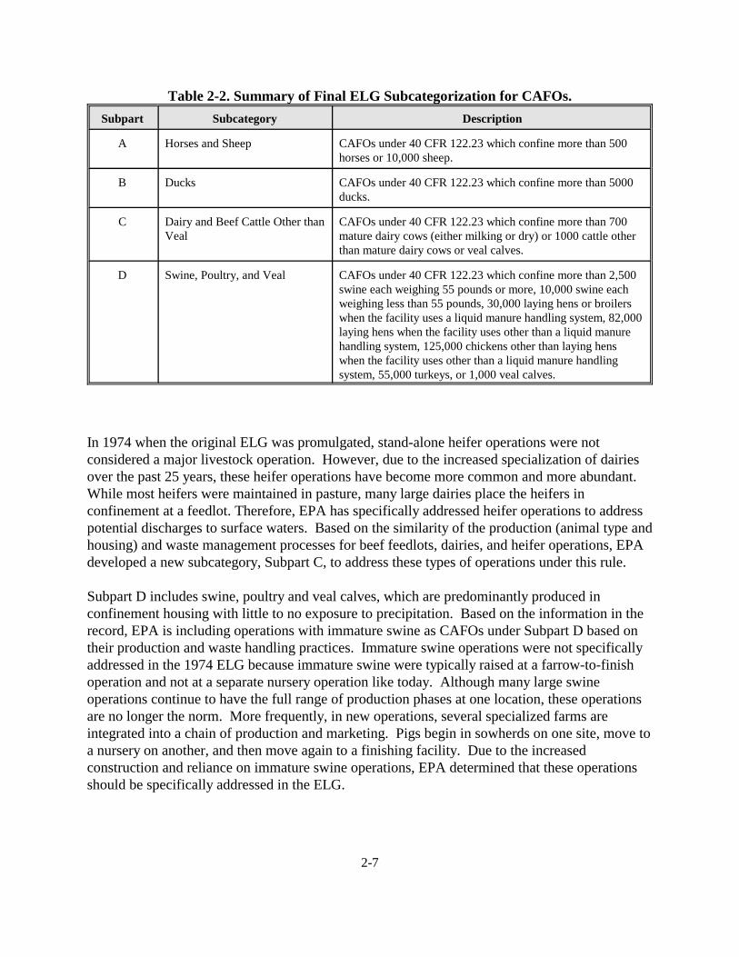
2-7

Table 2-2. Summary of Final ELG Subcategorization for CAFOs.

Subpart Subcategory Description

A Horses and Sheep CAFOs under 40 CFR 122.23 which confine more than 500 horses or 10,000 sheep.

B Ducks CAFOs under 40 CFR 122.23 which confine more than 5000ducks.

C Dairy and Beef Cattle Other thanVeal

CAFOs under 40 CFR 122.23 which confine more than 700mature dairy cows (either milking or dry) or 1000 cattle otherthan mature dairy cows or veal calves.

D Swine, Poultry, and Veal CAFOs under 40 CFR 122.23 which confine more than 2,500swine each weighing 55 pounds or more, 10,000 swine eachweighing less than 55 pounds, 30,000 laying hens or broilerswhen the facility uses a liquid manure handling system, 82,000laying hens when the facility uses other than a liquid manurehandling system, 125,000 chickens other than laying hens when the facility uses other than a liquid manure handlingsystem, 55,000 turkeys, or 1,000 veal calves.

In 1974 when the original ELG was promulgated, stand-alone heifer operations were notconsidered a major livestock operation. However, due to the increased specialization of dairiesover the past 25 years, these heifer operations have become more common and more abundant. While most heifers were maintained in pasture, many large dairies place the heifers inconfinement at a feedlot. Therefore, EPA has specifically addressed heifer operations to addresspotential discharges to surface waters. Based on the similarity of the production (animal type andhousing) and waste management processes for beef feedlots, dairies, and heifer operations, EPAdeveloped a new subcategory, Subpart C, to address these types of operations under this rule.

Subpart D includes swine, poultry and veal calves, which are predominantly produced inconfinement housing with little to no exposure to precipitation. Based on the information in therecord, EPA is including operations with immature swine as CAFOs under Subpart D based ontheir production and waste handling practices. Immature swine operations were not specificallyaddressed in the 1974 ELG because immature swine were typically raised at a farrow-to-finishoperation and not at a separate nursery operation like today. Although many large swineoperations continue to have the full range of production phases at one location, these operationsare no longer the norm. More frequently, in new operations, several specialized farms areintegrated into a chain of production and marketing. Pigs begin in sowherds on one site, move toa nursery on another, and then move again to a finishing facility. Due to the increasedconstruction and reliance on immature swine operations, EPA determined that these operationsshould be specifically addressed in the ELG.

2-8

The simplest approach for including immature swine is to count all swine, regardless of size andage. EPA determined counting all swine equally would increase the effective size of operationsthat have breeding functions by a factor of seven or more (based on the number of pigs per litter). While this approach would include nursery facilities, this approach also changes the existingbasis without improving the regulation. Alternatively, all swine would be counted but aweighting factor could be used to distinguish animal sizes. This approach is inconsistent withEPA’s attempt to simplify the regulations by removing mixed animal multipliers and animal unitcalculations.

EPA selected the approach of counting the numbers of mature swine and numbers of immatureswine separately, where either one of which could define the facility as a CAFO. EPA selectedphosphorus in the manure as the metric for Large CAFO thresholds. EPA’s analysis equates 2,500 mature swine (weighing over 55 pounds) to approximately 10,000 immature swine(weighing less than 55 pounds) on a phosphorus excreted basis. Once a swine facility is definedas a CAFO for either age group of animals, all animals in confinement would be considered aspart of the CAFO. Because the immature operations use virtually the same animal productionand waste management processes and are expected to use similar effluent reduction practices andtechnologies as mature swine operations, EPA has included these immature swine operationsunder Subpart D.

As discussed in Section 2.1, the final rule expands the scope of the rule to also address chickenoperations with “dry” litter management systems. While liquid manure systems continue to beused by approximately 15 percent of the total laying industry (see Chapter 4), continuous flowwatering systems have been largely discontinued in favor of more efficient water conservingmethods (e.g., on-demand watering). Site visits and consultations with industry further suggestliquid manure handling systems are no longer constructed at laying hen operations.

EPA noted chickens raised for meat production are a different breed of chicken, have a differentweight, eat a different diet, and are raised differently than those used for egg production. Therefore EPA considered a number of approaches to determine the final applicabilitythresholds. EPA evaluated the manure generated from chickens used for meat (broilers) and eggproduction (layers) and compared manure production to a 1,000 pound beef cow. EPA evaluateddaily manure phosphorus production and annual phosphorus production, and determined annualproduction was more appropriate because annual production reflects the time birds are actuallypresent and generating manure. The annual approach assumes 5 to 6 flocks of broilers areproduced each year, for a total of 322 days of manure production in one year. In contrast, eachlayer flock is raised for either 80 weeks (non-molt flocks) or 105 weeks (molt flocks). Moltflocks go through two cycles of egg production, separated by a non-productive molting period(shedding of feathers and renewal of ovarian activity) induced by withholding food. Manureproduction greatly diminishes during the two-week molt period. Following the molt, eggproduction resumes to the end of the flock life. Furthermore, prior to egg-laying age, the birdwill typically be raised for 19 weeks as a pullet. On average, layers are in production for 94weeks. EPA’s final evaluation concluded that 125,000 broilers and 82,000 layers produce anequivalent amount of manure phosphorus to 1,000 beef cows.

2-9

This rule addresses veal operations under Subpart D along with swine and poultry operations dueto the similarity in animal production and waste management processes. See Chapter 5 foradditional discussion of the industry subcategorization for this rule.

2.2.2 Summary of Revisions to Effluent Limitations Guidelines and Standards

Large CAFOs covered under Subpart C and Subpart D are required under this final rule tocomply with the new effluent limitations guidelines and standards (see Table 2-3). The finalguidelines establish BPT, BCT, BAT, and NSPS by requiring effluent limitations and standardsand specific BMP that ensure that manure storage and handling systems are inspected andmaintained adequately as described in the following subsections. Medium and Small CAFOs arenot subject to the ELGs.

2.2.2.1 Land Application Best Practicable Control Technology

EPA set BPTs for land application applicable to any CAFO subject to Subparts C or D. TheseBMPs include the requirement to develop and implement a nutrient management plan thatincorporates the following requirements based on a field-specific assessment:

• Determination of application rates. Application rates for manure, litter, and otherprocess wastewater applied to land under the ownership or operational control of theCAFO must minimize phosphorus and nitrogen transport from the field to surfacewaters in compliance with the technical standards for nutrient management establishedby the Director. Such technical standards for nutrient management shall:

- Include a field-specific assessment of the potential for nitrogen and phosphorustransport from the field to surface waters, and address the form, source, amount,timing, and method of application of nutrients on each field to achieve realisticproduction goals, while minimizing nitrogen and phosphorus movement tosurface waters; and

- Include appropriate flexibilities for any CAFO to implement nutrient managementpractices to comply with the technical standards, including consideration of multi-year phosphorus application on fields that do not have a high potential forphosphorus runoff to surface water, phased implementation of phosphorus-basednutrient management, and other components, as determined appropriate by theDirector.

• Manure and Soil Sampling. Manure must be analyzed a minimum of once annually fornitrogen and phosphorus content, and soil analyzed a minimum of once every five yearsfor phosphorus content. The results of these analyses are to be used in determiningapplication rates for manure, litter, and other process wastewater.

2-10

• Inspect land application equipment for leaks. The operator must periodically inspectequipment used for land application of manure, litter, or process wastewater.

• Setback requirements. Manure, litter, and process wastewater may not be applied closerthan 100 feet to any down-gradient surface waters, open tile line intake structures,sinkholes, agricultural well heads, or other conduits to surface waters unless one of thefollowing compliance alternatives are used:

- Vegetated buffer compliance alternative. As a compliance alternative, the CAFOmay substitute the 100-foot setback with a 35-foot wide vegetated buffer whereapplications of manure, litter, or process wastewater are prohibited.

- Alternative practices compliance alternative. As a compliance alternative, theCAFO may demonstrate that a setback or buffer is not necessary becauseimplementation of alternative conservation practices or field-specific conditionswill provide pollutant reductions equivalent or better than the reductions thatwould be achieved by the 100-foot setback.

• Record keeping requirements for the land application areas. Each CAFO mustmaintain on-site a copy of its site-specific nutrient management plan and the followinginformation for a period of five years from the date they are created:

- Expected crop yields.

- The date(s) manure, litter, or process waste water is applied to each field.

- Weather conditions at time of application and for 24 hours prior to and followingapplication.

- Test methods used to sample and analyze manure, litter, process waste water, andsoil.

- Results from manure, litter, process waste water, and soil sampling.

- Explanation of the basis for determining manure application rates, as provided inthe technical standards established by the Director.

- Calculations showing the total nitrogen and phosphorus to be applied to eachfield, including sources other than manure, litter, or process wastewater.

- Total amount of nitrogen and phosphorus actually applied to each field, includingdocumentation of calculations for the total amount applied.

- The method used to apply the manure, litter, or process wastewater.

2-11

- Date(s) of manure application equipment inspection.

2.2.2.2 Production Area Best Practicable Control Technology

EPA set BPTs for the production area that are applicable to any CAFO subject to Subparts C orD. Under BPT, EPA prohibits the discharge of manure, litter, or process wastewater pollutantsinto waters of the United States from the production area except overflow from containmentfacilities if caused by rainfall events and the facility is designed, constructed, operated, andmaintained to contain all manure, litter, and process wastewater including the runoff and thedirect precipitation from a 25-year, 24-hour rainfall event. The production area must also beoperated in accordance with the additional measures and record keeping requirements describedbelow. These requirements do not apply to discharges to ground water with a direct hydrologicconnection to surface water, although the permit writer could establish such technology-basedlimitations on a case-by-case basis. BPT establishes the following additional measures andrecord keeping requirements for the production area (records are to be kept for five years fromthe time they are created):

• Weekly inspections of all storm water diversion devices, runoff diversion structures, anddevices channelling contaminated storm water to the wastewater and manure storageand containment structure.

• Daily inspection of water lines, including drinking water or cooling water lines.

• Weekly inspections of the manure, litter, and process wastewater impoundments; theinspection will note the level in liquid impoundments as indicated by the depth marker.

• All open surface liquid impoundments must have a depth marker which clearly indicatesthe minimum capacity necessary to contain the runoff and direct precipitation of the 25-year 24-hour rainfall event.

• Any deficiencies found as a result of these inspections must be corrected as soon aspossible.

• Mortalities must not be disposed of in any liquid manure or process wastewater system,and must be handled in such a way as to prevent the discharge of pollutants to surfacewater, unless alternative technologies are designed and approved to handle mortalities.

• Records documenting the inspections described above.

• Weekly records of the depth of the manure and process wastewater in the liquidimpoundment as indicated by the depth marker.

• Records documenting any actions taken to correct deficiencies described above.Deficiencies not corrected within 30 days must be accompanied by an explanation of thefactors preventing immediate correction.

• Records of mortalities management and practices used by the CAFO to meet therequirements described above.

2-12

• Records documenting the current design of any manure or litter storage structures,including volume for solids accumulation, design treatment volume, total designvolume, and approximate number of days of storage capacity.

• Records of the date, time, and estimated volume of any overflow.

EPA set an alternative BPT, described in section 2.2.2.6 below, to encourage innovativetechnologies.

2.2.2.3 Best Control Technology

EPA set BCT requirements for Subparts C (dairy and beef cattle other than veal subcategories)and D (swine, poultry, and veal subcategories) the same as BPT. Table 2-3 shows the technologybasis of BCT for these subcategories.

2.2.2.4 Best Available Technology

EPA set BAT requirements for Subparts C (dairy and beef cattle other than veal subcategories)and D (swine, poultry, and veal subcategories) the same as BPT. Table 2-3 shows the technologybasis of BAT for these subcategories.

2.2.2.5 New Source Performance Standards

EPA set NSPS requirements equivalent to BPT requirements for Subpart C (dairy and beef cattleother than veal subcategories) and for the land application area of Subpart D (swine, poultry, andveal subcategories).

EPA set different NSPS requirements for the production area of Subpart D (swine, poultry, andveal subcategories). NSPS requirements for Subpart D prohibit the discharge of manure, litter, orprocess wastewater pollutants into waters of the United States from the production area. Afacility designed, constructed, operated, and maintained to contain all manure, litter, and processwastewater including the runoff and the direct precipitation from a 100-year, 24-hour rainfallevent will fulfill the requirement for no discharge. The production area must also be operated inaccordance with the additional measures and record keeping requirements described earlier withthe exception that all open surface liquid impoundments must have a depth marker which clearlyindicates the minimum capacity necessary to contain the runoff and direct precipitation of the100-year 24-hour rainfall event.

EPA set an alternative NSPS, described in Section 2.2.2.7 below, to encourage innovativetechnologies and whole-farm multi-media reductions.

For the purposes of applying the new source performance standards, a source is a new source if itcommenced construction after the effective date of the final rule. See 40 CFR 122.2. Eachsource that meets this definition is required to achieve the newly promulgated NSPS uponcommencing discharge.

2-13

Tab

le 2

-3. S

umm

ary

of T

echn

olog

y B

asis

for

Lar

ge C

AF

Os

Cov

ered

by

Par

t 41

2.

Tec

hnol

ogy

Bas

is

BP

T, B

CT

, and

BA

TN

SPS

Dai

ry a

nd B

eef

Cat

tle

othe

rT

han

Vea

lSu

bcat

egor

y

Swin

e,P

oult

ry, a

ndV

eal

Subc

ateg

ory

Dai

ry a

nd B

eef

Cat

tle

othe

rT

han

Vea

lSu

bcat

egor

y

Swin

e,P

oult

ry, a

ndV

eal

Subc

ateg

ory

Zer

o di

scha

rge

wit

h ov

erfl

ow p

rovi

ded

if c

ause

d by

rai

nfal

l eve

nts

and

the

faci

lity

is d

esig

ned,

con

stru

cted

, ope

rate

d, a

nd m

aint

aine

d to

con

tain

all m

anur

e, li

tter

, and

pro

cess

was

tew

ater

incl

udin

g th

e ru

noff

and

the

dire

ct p

reci

pita

tion

fro

m a

25-

year

, 24-

hour

rai

nfal

l eve

nt.

TT

T

Zer

o di

scha

rge

wit

h ov

erfl

ow p

rovi

ded

if c

ause

d by

rai

nfal

l eve

nts

and

the

faci

lity

is d

esig

ned,

con

stru

cted

, ope

rate

d, a

nd m

aint

aine

d to

con

tain

all m

anur

e, li

tter

, and

pro

cess

was

tew

ater

incl

udin

g th

e ru

noff

and

the

dire

ct p

reci

pita

tion

fro

m a

100

-yea

r, 2

4-ho

ur r

ainf

all e

vent

.

T

Dev

elop

men

t an

d im

plem

enta

tion

of

a nu

trie

nt m

anag

emen

t pl

an;

and

mai

ntai

n re

cord

s.T

TT

T

Lan

d ap

plic

atio

n co

nsis

tent

wit

h ap

prop

riat

e ag

ricu

ltur

al u

tiliz

atio

n.T

TT

T

Vol

unta

ry a

lter

nati

ve p

erfo

rman

ce s

tand

ards

for

dis

char

ges

from

the

prod

ucti

on a

rea

that

ach

ieve

equ

al o

r be

tter

pol

luta

nt r

educ

tion

.T

TT

Vol

unta

ry s

uper

ior

envi

ronm

enta

l per

form

ance

sta

ndar

ds f

orte

chno

logi

es t

hat

achi

eve

over

all e

nvir

onm

enta

l per

form

ance

acr

oss

all

med

ia e

qual

or

supe

rior

to

base

line

NS.

PS

T

Dai

ly a

nd w

eekl

y in

spec

tion

s.T

TT

T

Dep

th m

arke

r fo

r op

en s

urfa

ce li

quid

impo

undm

ents

.T

TT

T

Cor

rect

ive

acti

on.

TT

TT

Mor

talit

y ha

ndlin

g re

quir

emen

ts.

TT

TT

100-

foot

land

app

licat

ion

setb

ack

or e

quiv

alen

t co

mpl

ianc

e al

tern

ativ

e.T

TT

T

Man

ure

sam

ples

at

leas

t on

ce p

er y

ear.

TT

TT

Soil

test

eve

ry 5

yea

rs.

TT

TT

Rec

ord

keep

ing.

TT

TT

2-14

However, the NSPS promulgated in 1974 continue to have force and effect for a limited universeof new sources; for this reason, in the final rule, EPA is including provisions at 40 CFR412.35(d) and 412.46(e) addressing this limited universe. Specifically, the NSPS established in1974 will continue to apply for a limited period of time to new sources that completedconstruction with the time period beginning ten years before the effective date of this rule andending on the effective date of this rule. Thus, any direct discharging new source that completedconstruction during this ten year period is subject to the 1974 NSPS for ten years from the date itcompleted construction or during the period of depreciation or amortization of such facility,whichever comes first. See CWA section 306(d). After that ten-year period expires, the BPT,BCT, and BAT limitations established in this rule apply because they are more stringent than the1974 NSPS.

EPA has determined that the ten-year period should apply to discharges from the both the CAFOproduction areas and land application areas even though the 1974 NSPS specifically addressedonly discharges from the production area. This determination is based on the manner in whichmanure, litter, and other process wastewaters at CAFOs are generated and the waste managementpractices employed for these wastes. EPA recognizes that the land application BMPs establishedby this rule have the potential to alter the land application practices at the CAFO, which couldaffect waste management practices at the production area. Animal feeding strategies and wastemanagement practices at the production area determine the form of the wastes (i.e., solid, liquid,or slurry) and the amount of nutrients and other pollutants present in the wastes. The timing ofany application and the amount of nutrients (i.e., manure, litter, and other process wastewater)applied is determined by crop needs, irrigation requirements, and other factors such as theavailability of manure spreading equipment and climate considerations. The land applicationBMPs established by this rule include a requirement to develop and implement a nutrientmanagement plan, as well as a requirement to land-apply manure at rates based on technicalstandards for nutrient management established by the Director. Based on the information in therecord, the land application BMPs established by this rule will lead to some changes in the waysCAFOs manage their land application areas. A number of CAFOs affected by this rule will needto reduce the amount of manure and other process wastewaters applied to cropland. As theydevelop their nutrient management plans some CAFOs may determine they should adjust thetiming of manure applications. Since the CAFO must be able to store any wastes generated at theproduction area until able to land-apply the manure, significant changes in the amount of manureapplied or the timing of manure application may affect waste management systems at theproduction area. Therefore, EPA determined that the ten-year period described above shouldapply to discharges from both the production areas and the land application areas at CAFOs.

If the production area and land application area wastestreams at CAFOs were more physicallydistinct, particularly if they were generated and remained distinct and severable throughout allsteps of the waste generation and management (or could be managed in such a manner), and theNSPS requirements for the land application area did not significantly affect the wastemanagement infrastructure at the production area, EPA likely would have determined that theten-year “grandfathering” period would apply only to production area discharges and would notapply to discharges from the land application areas.

2-15

Rather than reproduce the 1974 NSPS in the newly revised rule, EPA is referring permittingauthorities to the NSPS codified in the 2002 edition of the Code of Federal Regulations for useduring the applicable ten-year period. (The 2002 edition of the Code of Federal Regulationspresents the 1974 NSPS requirements.) This approach allows EPA to avoid reproducing in thenew regulations the requirements of the 1974 NSPS that will soon become outdated.

2.2.2.6 Voluntary Alternative Performance Standards to Encourage InnovativeTechnologies

In addition to the production area effluent guidelines (baseline effluent guidelines), the final ruleestablishes provisions for the development of alternative performance standards for dischargesfrom the production area for existing Large CAFOs and new Large beef and dairy CAFOs. TheBMPs described under BPT are applicable to all Large CAFOs (both existing and new sources),regardless of whether their NPDES permit limitations are based on the baseline effluentguidelines or the alternative performance standards.

The voluntary alternative performance standards will enable Large CAFOs to develop andimplement new technologies and management practices that perform as well as or better than thebaseline effluent guidelines at reducing pollutant discharges to surface waters from theproduction area. CAFOs will have the option to either accept NPDES permit limitations based onthe baseline effluent guidelines, or may voluntarily request the permitting authority to establishan alternative BPT/BCT/BAT/NSPS performance standard as the basis for their technology-based NPDES permit limits. The specific requirements imposed by the alternative performancestandard would be established by the NPDES permitting authority on the basis of BPJ.

Under this program, CAFOs will be allowed to discharge process wastewater that has beentreated by technologies that the CAFO demonstrates will result in equivalent or better pollutantremoval than would otherwise be achieved by the baseline effluent guidelines. These regulatoryprovisions are targeted toward the CAFO’s wastewater discharges, but EPA encouragesoperations electing to participate in the alternative performance standards program to considerenvironmental releases holistically and also consider opportunities for achieving improvement inmultiple environmental media. To demonstrate that an alternative control technology wouldachieve equivalent or better pollutant reductions than baseline effluent guidelines, the CAFOmust submit a technical analysis, which includes calculating the quantity of pollutant reductions,on a mass-basis where appropriate, based on the site-specific modeled performance of a systemdesigned to comply with the baseline effluent guidelines. The CAFO must also prepare aproposed alternative program plan including the results of the analysis; the proposed method forimplementing new technologies and practices, including an approach for monitoringperformance; and the results demonstrating that these technologies and practices performequivalent to or better than the baseline effluent guidelines. This plan must be included with theCAFO’s NPDES permit application or renewal, and will be incorporated into the permit uponapproval by the permitting authority.

2-16

2.2.2.7 Voluntary Superior EnvironmentalPerformance Standards for New LargeSwine/Poultry/Veal CAFOs

The NSPS requirements that apply to production area discharges at new Large swine, poultry,and veal CAFOs are more stringent than the NSPS established for other new sources and theBAT requirements for existing sources. EPA is endeavoring to ensure that this rule does notinadvertently discourage approaches that are superior from a multi-media environmentalperspective. Therefore, for new sources subject to Subpart D (Large swine, poultry, and vealCAFOs), EPA is establishing alternative performance standards that provide additionalcompliance flexibilities specifically designed to encourage CAFOs to adopt innovativetechnologies for managing and/or treating manure, litter, and process wastewater. Specifically,alternative NPDES permit limitations based upon a demonstration that site-specific innovative orsuperior to the reductions achieved by baseline standards. The quantity of pollutants dischargedfrom the production area must be accompanied by an equivalent or greater reduction in thequantity of pollutants released to other media from the production are (e.g., air emissions formhousing and storage), the land application areas for all manure, litter, and process wastewater aton-site and off-site locations, or both. In making the demonstration that the innovativetechnologies will achieve an equivalent or greater reduction, the comparison of quantity ofpollutants is to be made on a mass basis where appropriate.

In general, EPA expects CAFOs will conduct a whole-farm audit to evaluate releases that occurat the point to generation to minimize or eliminate waste production and air emissions, followedby an evaluation of the waste handling and management systems, and ending with an evaluationof land application and offsite transfer operations. The specific technologies that CAFOs willselect and adopt to achieve the pollutant reductions are expected to be most effective for theparticular operation. As part of the demonstration the CAFO will need to present information thatdescribes how the innovative technologies will generate improvement across multipleenvironmental media. The Director has the discretion to request additional supportinginformation to supplement such a request where necessary. Such information could includecriteria and data that demonstrate effective performance of the technologies and that could beused to establish the alternative NPDES permit limitations.

3-1

CHAPTER 3

DATA COLLECTION ACTIVITIES

3.0 DATA COLLECTION ACTIVITIES

EPA collected and evaluated data from a variety of sources during the course of developing therevised effluent limitations guidelines and standards for the CAFO industry. These data sourcesinclude EPA site visits, industry trade associations, the U.S. Department of Agriculture (USDA),published literature, previous EPA Office of Water studies of the Feedlots Point SourceCategory, and other EPA studies of AFOs. Each of these data sources is discussed below, andanalyses of the data collected by EPA are presented throughout the remainder of this document.

The majority of the data EPA used to support development of the proposed effluent limitationsguidelines and standards for the CAFO industry are from existing sources, including data fromthe USDA, industry, State agricultural extension agencies, and several land grant universities. As defined in the Office of Water 2002 Quality Management Plan, existing (or secondary) dataare data that were not directly generated by EPA to support the decision at hand.

In keeping with the graded approach to quality management embodied in the Office of Water'squality management plan, EPA must assess the quality of existing data relative to their intendeduse. The procedures EPA used to assess existing data for use in developing effluent guidelinelimitations for CAFOs varied with the specific type of data. In general, EPA's assessmentincluded:

• Reviewing a description of the existing data that explains who collected or produced thedata and how the data were collected or produced (e.g., who collected the data, whatdata were collected; why were the data originally collected; when were the datacollected; how were they collected; are the data part of a long-term collection effort, orwas this a one-time effort; who else uses the data; what level of review by others havethe data undergone).

• Specifying the intended use of the existing data relative to the CAFO final rule.

• Developing a rationale for accepting data from this source, either as a set of acceptancecriteria, or as a narrative discussion.

• Describing any known limitations with the data and their impact on EPA's use of thedata.

Brief descriptions of the data and their limitations are presented later in this document, as eachdata source is introduced.

3-2

In searching for existing data sources and determining their acceptability, EPA generally used ahierarchical approach designed to identify and utilize data with the broadest representation of theindustry sector of interest. EPA began by searching for national-level data from surveys andstudies by USDA and other federal agencies. When such survey or study data did not exist, EPAconsidered other data from federal agencies. An example of non-survey data considered are theUSDA costs and capability data, which are based on a consensus of USDA experts.

Where national data did not exist, as the second tier, EPA searched for data from land grantuniversities. Such data are often local or regional in nature. EPA assessed the representativenessof the data relative to a national scale before deciding to use the data. When such data camefrom published sources, EPA gave greater consideration to publications in peer-reviewedprofessional journals compared to trade publications that do not have a formal review process.

The third tier was data supplied by industry. Prior to proposal, EPA requested data from avariety of industry sources, including trade associations and large producers. The level of reviewapplied to data supplied by industry depended on the level of supporting detail that was provided. For example, if the industry supplied background information regarding how the data werecollected, such as the number of respondents and the total number of potential respondents, EPAreviewed the results, compared them to data from other potential sources to determine theirsuitably for use in this rulemaking. If the data provided by industry originated from anidentifiable non-industry source (e.g., a state government agency), EPA reviewed the originalsource information before determining the acceptability of the data. In a limited number ofinstances, EPA conducted site visits to substantiate information supplied by industry. In contrast,data supplied by industry without any background information were given much less weight andgenerally were not used by EPA. Further, some data that were supplied by industry prior to theproposal were included in the proposal for comment. In the absence of any negative comments,such data were relied on to a greater extent than data submitted by industry during the commentperiod itself.

3.1 Summary of EPA’s Site Visit Program

EPA conducted approximately 116 site visits to collect information about AFOs and wastemanagement practices. Specifically, EPA visited beef feedlots, dairies, and swine, poultry, andveal operations throughout the United States. A wide range of operations were visited includingthose demonstrating centralized treatment or new and innovative technologies. EPA chose themajority of facilities with the assistance of the following industry trade associations:

• National Pork Producers Council

• United Egg Producers and United Egg Association

• National Turkey Federation

• National Cattlemen’s Beef Association

3-3

• National Milk Producers Federation

• Western United Dairymen

EPA also received assistance from environmental groups, such as the Natural Resources DefenseCouncil and the Clean Water Network. The Agency contacted university experts, statecooperatives and extension services, and state and EPA regional representatives when identifyingfacilities for site visits. EPA also attended USDA-sponsored farm tours, as well as industry,academic, and government conferences.

Table 3-1 summarizes the number of site visits EPA conducted by animal industry sector, sitelocations, and size of animal operations.

Table 3-1. Number of Site Visits Conducted by EPA for the Various Animal Industry Sectors.

AnimalSector

Number of SiteVisits Location(s) Size of Operations

Swine 30 NC, PA, OH, IA, MN, TX, OK, UT 900–1 million head

Poultry 6 (broiler)GA, AR, NC, VA, WV, MD, DE, PA,

OH, IN, WI20,000–1 million birds12 (layer)

6 (turkey)

Dairy 29 PA, FL, CA, WI, CO, VA 40–4,000 cows

Beef 30 TX, OK, KS, CO, CA, IN, NE, IA 500–120,000 head

Veal 3 IN 500–540 calves

EPA considered the following factors when identifying representative facilities for site visits:

• Type of animal feeding operation

• Location

• Feedlot size

• Current waste management practices

Facility-specific selection criteria are contained in site visit reports (SVRs) prepared for eachfacility visited by EPA. The SVRs are located in the administrative record for this rulemaking.

During the site visits, EPA typically collected the following types of information:

• General facility information including size and age of facility, number of employees,crops grown, precipitation information, and proximity to nearby waterways.

3-4

• Animal operation data including flock or herd size, culling rate, and method fordisposing of dead animals.

• Description of animal holding areas such as barns or pens, and any central areas, such asmilking centers.

• Manure collection and management information including the amount generated,removal methods and storage location, disposal information, and nutrient content.

• Wastewater collection and management information including the amount generated,runoff information, and nutrient content.

• Nutrient management plans and BMPs.

• Available wastewater discharge permit information.

This information, along with other site-specific information, is documented in the SVRs for eachfacility visited.

3.2 Industry Trade Associations

EPA contacted the following industry trade associations and representatives during thedevelopment of the proposed and promulgated rules.

US Poultry and Egg Association (USPOULTRY). USPOULTRY is described in their literatureas dedicated to the growth, progress, and welfare of the poultry industry and all of its individualand corporate interests. All segments of the industry are represented, from producers of eggs,turkeys, and broilers to the processors of these products and allied companies which serve theindustry. USPOULTRY sponsors the world's largest poultry industry show; scientific research;and a comprehensive, year-round educational program for members of the industry.

Capitol Link. Capitol Link represents the interests of many livestock organizations and acts as aliaison with federal agencies such as EPA. They frequently provide comments and data onproposed federal regulatory actions.

National Pork Producers Council (NPPC). NPPC is a marketing organization and tradeassociation made up of 44 affiliated state pork producer associations. NPPC’s stated purpose isto increase the quality, production, distribution, and sales of pork and pork products.

United Egg Producers and United Egg Association (UEP/UEA). UEP/UEA promotes the eggindustry in the following areas: price discovery, production and marketing information, unifiedindustry leadership, USDA relationships, and promotional efforts.

National Turkey Federation (NTF). NTF describes itself as the national advocate for allsegments of the turkey industry, providing services and conducting activities that increasedemand for its members’ products.

3-5

National Chicken Council (NCC) and National Broiler Council (NBC). NCC is a tradeassociation representing the vertically integrated companies that produce and process about 95percent of the chickens sold in the United States. The association provides consumer education,public relations, and public affairs support, and is working to seek a positive regulatory,legislative, and economic environment for the broiler industry. The NCC’s activities generallyreplace those activities conducted prior to proposal by the National Broiler Council.

National Cattlemen’s Beef Association (NCBA). NCBA is a marketing organization and tradeassociation for cattle farmers and ranchers, representing the beef industry.

National Milk Producers Federation (NMPF). NMPF is involved with milk quality andstandards, animal health and food safety issues, dairy product labeling and standards, andlegislation affecting the dairy industry.

American Veal Association (AVA). AVA represents the veal industry, advances the industry’sconcerns in the legislative arena, coordinates production-related issues affecting the industry, andhandles other issues relating to the industry.

Western United Dairymen (WUD). WUD, a dairy organization in California, promoteslegislative and administrative policies and programs for the industry and consumers.

Professional Dairy Heifer Growers Association (PDHGA). PDHGA is an association of heifergrowers dedicated to growing high-quality dairy cow replacements. The association offerseducational programs and professional development opportunities, provides a communicationnetwork, and establishes business and ethical standards for the dairy heifer grower industry.

All of the above organizations, along with several of their state affiliates, assisted EPA’s effortsto understand the industry by helping with site visit selection, submitting supplemental data, andreviewing descriptions of the industry and waste management practices. These organizationsalso participated in and hosted meetings with EPA for the purpose of exchanging information. EPA also obtained copies of membership directories and conference proceedings, which wereused to identify contacts and obtain additional information on the industry. Publications fromtrade associations were used to support cost methodologies.

3.3 U.S. Department of Agriculture

EPA obtained data from several agencies within the USDA, including the National AgriculturalStatistics Service (NASS), the Animal and Plant Health Inspection Service (APHIS), NaturalResources Conservation Service (NRCS), and the Economic Research Service (ERS) in order tobetter characterize the CAFO industry. The collected data include statistical survey informationand published reports. Data collected from each agency are described below.

3-6

3.3.1 National Agricultural Statistics Service

NASS is responsible for objectively providing accurate statistical information and data supportservices of structure and activities of agricultural production in the United States. Each yearNASS conducts hundreds of surveys and prepares reports covering virtually every facet of U.S.agricultural publications. The primary source of data is the animal production facility. NASScollects voluntary information using mail surveys, telephone and in-person interviews, and fieldobservations. NASS is also responsible for conducting a Census of Agriculture every 5 years. EPA gathered information from the following published NASS reports:

• 1997 Census of Agriculture

• Hogs and Pigs: Final Estimates 1993 - 1997

• Chickens and Eggs: Final Estimates 1994 - 1997

• Poultry Production and Value: Final Estimates 1994 - 1997

• Cattle: Final Estimates 1994 - 1998

• Milking Cows and Production: Final Estimates 1993 - 1997

The information EPA collected from these sources is summarized below.

1997 Census of Agriculture

The Census of Agriculture is a complete accounting of U.S. agricultural production and is theonly source of uniform, comprehensive agricultural data for every county in the nation. Thecensus is conducted every 5 years. The Bureau of the Census conducted this activity until 1997,when the responsibility passed to NASS. The census includes all farm operations from which$1,000 or more of agricultural products are produced and sold. The most recent census occurredin late 1997 and is based on calendar year 1997 data.

The census collects information relating to land use and ownership, crops, livestock, and poultry. USDA maintains this database; EPA compiled data used for this analysis with the assistance ofNASS staff. (USDA periodically publishes aggregated data from these databases and alsocompiles customized analyses of the data for members of the public and other governmentagencies. In providing such analyses, USDA maintains a sufficient level of aggregation to ensurethe confidentiality of any individual operation’s activities or holdings.)

EPA developed several size groups to allow tabulation of farm counts by farm size usingdifferent criteria than those used in the published 1997 Census of Agriculture. EPA developedalgorithms to define farm size in terms of capacity, or number of animals likely to be found onthe farm at any given time. To convert sales of hogs and pigs and feeder pigs into an inventory,EPA divided total sales by the number of groups of pigs likely to be produced and sold in a givenyear. EPA estimates that the larger grower-finisher farms produce 2.8 groups of pigs per year.

3-7

Farrow-to-finish operations produce 2.0 groups of pigs per year. Nursery operations produce upto 10 groups per year. EPA developed data used to determine the groups of pigs produced peryear from a survey conducted by APHIS (USDA,1999). For beef feedlots, EPA worked withstaff from NASS and NCBA to estimate the number of groups of cattle produced per year at aCAFO, and the capacity of the operation based on the number of cattle sold. EPA estimates thatbeef feedlots produce between 1 and 2.5 groups of cattle per year, depending on the size of theoperation (ERG, 2002).

Hogs and Pigs: Final Estimates 1993 - 1997

EPA used data from this report to augment the swine industry profile. The report presentsinformation on inventory, market hogs, breeding herds, and pig crops, and specifically, thenumber of farrowings, sows, and pigs per litter. This report presents the number of operationswith hogs; however, EPA did not use this information to estimate farm counts because the reportprovided limited data. Instead, as discussed earlier in this section, EPA used data provided byUSDA based on the 1997 Census of Agriculture.

Chickens and Eggs: Final Estimates 1994 - 1997

EPA used data from this report to augment the poultry industry profile. The report presentsnational and state-level data for the top-producing states on chickens and eggs including thenumber laid, and production for 1994 through 1997.

Poultry Production and Value: Final Estimates 1994 - 1997

EPA used data from this report to augment the poultry industry profile. The report presentsnational and state-level data for the top-producing states on production (number and poundsproduced/raised), price per pound or egg, and value of production of broilers, chickens, eggs, andturkeys for 1994 through 1997.

Cattle: Final Estimates 1994 - 1998

EPA used data from this report to augment the beef industry profile. The report provides thenumber of and population estimates for beef feedlots that have a capacity of over 1,000 head ofcattle, grouped by size and geographic distribution. This report also provides national and state-level data which include the number of feedlots, cattle inventory, and number of cattle sold peryear by size class for the 13 top-producing beef states. In addition, the report presents the totalnumber of feedlots that have a capacity of fewer than 1,000 head of cattle, total cattle inventory,and number of cattle sold per year for these operations. However, EPA did not use this report toestimate farm counts because it provided limited data. Instead, as discussed earlier in thissection, EPA used data provided by USDA based on the 1997 Census of Agriculture.

3-8

Milking Cows and Production: Final Estimates 1993 - 1997

EPA used data from this report to augment the dairy industry profile. The report presentsnational and state-level estimates of dairy cattle inventory and the number of dairy operations bysize group. This particular report presents data for all dairy operations with over 200 maturedairy cattle in one size class. However, EPA did not use this report to estimate farm countsbecause it provided limited data. Instead, as discussed earlier in this section, EPA used dataprovided by USDA based on the 1997 Census of Agriculture.

3.3.2 Animal and Plant Health Inspection Service National Animal Health MonitoringSystem (NAHMS)

APHIS provides leadership in ensuring the health and care of agricultural animals and plants,improving agricultural productivity and competitiveness, and contributing to the nationaleconomy and public health. One of its main responsibilities is to enhance the care of animals. In1983, APHIS initiated NAHMS as an information-gathering program to collect, analyze, anddisseminate data on animal health, management, and productivity across the United States. NAHMS conducts national studies to gather data and generate descriptive statistics andinformation from data collected by other industry sources. NAHMS has published national studyreports for various food animal populations (e.g., swine, dairy cattle).

EPA gathered information from the following NAHMS reports:

• Swine ’95 Part I: Reference of 1995 Swine Management Practices

• Swine ’95 Part II: Reference of Grower/Finisher Health & Management Practices

• Swine 2000 Part I: Reference of Swine Health and Management in the United States

• Layers ’99 Parts I and II: Reference of 1999 Table Egg Layer Management in the U.S.

• Dairy ’96 Part I: Reference of 1996 Dairy Management Practices

• Dairy ’96 Part III: Reference of 1996 Dairy Health and Health Management

• Beef Feedlot ’95 Part I: Feedlot Management Practices

• Feedlot ’99 Part I: Baseline Reference of Feedlot Management Practices

• Equine ’98 Parts I and II: Baseline Reference of 1998 Equine Health and Management

EPA also collected information from NAHMS fact sheets, specifically the Swine ’95 fact sheets,which describe biosecurity measures, vaccination practices, environmental practices/management, and antibiotics used in the industry. The information EPA collected from thesereports is summarized below.

3-9

Swine ’95 Part I: Reference of 1995 Swine Management Practices

This report (USDA APHIS, 1995b) provides references on productivity, preventative andvaccination practices, biosecurity issues, and environmental programs (including carcassdisposal). The data were obtained from a sample of 1,477 producers representing nearly 91percent of the U.S. hog inventory from the top 16 pork-producing states. Population estimatesare broken down into farrowing and weaning, nursery, grower/finisher, and sows.

Swine ’95 Part II: Reference of Grower/Finisher Health & Management Practices

This report (USDA APHIS, 1996a) provides additional references on feed and wastemanagement, health and productivity, marketing, and quality control. The data were collectedfrom 418 producers with operations having 300 or more market hogs (at least one hog over 120pounds) and represent about 90 percent of the target population. NAHMS also performedadditional analyses for EPA that present manure management information for the swine industryin two size classes (fewer than 2,500 marketed head and more than 2,500 marketed head) andthree regions (Midwest, North, and Southeast) (USDA APHIS, 1999).

Swine 2000 Part I: Reference of Swine Health and Management in the United States

Swine 2000 (USDA APHIS, 2001) was designed to statistically sample from operations with 100or more pigs. The study included 17 of the major pork-producing states that account for 94percent of the U.S. pig inventory. Data for this report were collected from 2,328 operations. This report provides information on feed and waste management, health and productivity, animalmanagement, and facility management. In addition to this report, NAHMS also performedadditional analyses for EPA that present the percent of sites where pit holding was the wastemanagement system used most by region and herd size for farrowing and grow/finish operations(USDA APHIS, 2002b).

Layers ’99 Parts I and II: Reference of 1999 Table Egg Layer Management in the U.S.

The Layers ’99 study (USDA APHIS, 2000b) is the first NAHMS national study of the layerindustry. Data were obtained from 15 states, which account for over 75 percent of the table egglayers in the United States. Part I of this report summarizes the study results includingdescriptions of farm sites and flocks, feed, and health management. Part II of this reportsummarizes biosecurity, facility management, and manure handling practices.

Dairy ’96 Part I: Reference of 1996 Dairy Management Practices and Dairy ‘96 Part III:Reference of 1996 Dairy Health and Health Management

These reports (USDA APHIS, 1996b and 1996c) present the results of a survey distributed todairies in 20 major states to collect information on cattle inventories; dairy herd managementpractices; health management; births, illness, and deaths; housing; and biosecurity. The resultsrepresent 83 percent of U.S. milk cows, or 2,542 producers. The reports also provide national

3-10

data on cattle housing, manure and runoff collection practices, and irrigation/land applicationpractices for dairies with more than, or fewer than, 200 mature dairy cattle. NAHMS providedthe same information to EPA with the results reaggregated into three size classes (fewer than500, 500 to 699, and more than 700 mature dairy cattle) and into three regions (East, West, andMidwest) (USEPA, 2002a).

Beef Feedlot ’95 Part I: Feedlot Management Practices

This report (USDA APHIS, 1995a) contains information on population estimates, environmentalprograms (e.g., ground water monitoring and methods of waste disposal), and carcass disposal atsmall and large beef feedlots (fewer than and more than 1,000 head capacity). The data werecollected from 3,214 feedlots in 13 states, representing almost 86 percent of the U.S. cattle-on-feed inventory.

Feedlot ’99 Part I: Baseline Reference of Feedlot Management Practices

This report (USDA APHIS, 2000a) contains information on population estimates, environmentalprograms, and carcass disposal at beef feedlots. The data were collected from 1,250 feedlots in12 states, representing 77 percent of all cattle on feed in the United States.

Equine ’98 Parts I and II: Baseline Reference of 1998 Equine Health and Management

This report contains information on population demographics, as well as health and healthmanagement practices. Part II of the same report describes nutrition, pasture, housing, bedding,and manure management. NAHMS performed additional analyses for EPA to provideinformation on primary use and function by size class (USDA APHIS, 2002a).

3.3.3 Natural Resources Conservation Services

NRCS provides leadership in a partnership effort to help people conserve, improve, and sustainU.S. natural resources and the environment. NRCS relies on many partners to help setconservation goals, work with people on the land, and provide assistance. Its partners includeconservation districts, state and federal agencies, NRCS Earth Team volunteers, agricultural andenvironmental groups, and professional societies.

NRCS publishes the Agricultural Waste Management Field Handbook (AWMFH) (USDANRCS, 1992), which is an agricultural/engineering guidance manual that explains general wastemanagement principles and provides detailed design information for particular wastemanagement systems. The handbook presents specific design information on a variety of farmproduction and waste management practices at different types of feedlots. The handbook alsoprovides runoff calculations under normal and peak precipitation as well as information onmanure and bedding characteristics. NRCS also publishes Conservation Practice Standards formany waste handling and treatment operations. EPA used this information to develop its costand environmental analyses. NRCS personnel also contributed technical expertise in the

3-11

development of EPA’s estimates of compliance costs and environmental assessment frameworkby providing EPA with estimates of manure generation in excess of expected crop uptake.

NRCS also analyzed the census data that EPA used for its analysis. In the draft February 23,2002 Profile of Farms with Livestock in the United States: A Statistical Summary (USDA, 2002),NRCS presents estimates of the number of CAFOs by animal sector and size group, as well asthe number of head at these farms. EPA used these estimates to calculate the average number ofhead and the number of CAFOs by animal sector and size group. In the case of beef feedlots,NRCS used a turnover rate of 2.5 to estimate capacity for all size operations. EPA recalculatedthe number of head at these operations using the turnover rates discussed above.

Another NRCS report (USDA, 2000), Manure Nutrients Relative to the Capacity of Croplandand Pastureland to Assimilate Nutrients: Spatial and Temporal Trends for the United Statespublished in December 2000, provides background information on trends in animal agricultureand manure production based on information collected in the 1997 Census of Agriculture. EPAused data on the percentage of farms with sufficient cropland, insufficient cropland, and nocropland to determine the number of CAFOs that require off-site transport of excess manure. EPA also used data from this report to determine the amount of excess manure at operations withan insufficient amount of cropland to agronomically land-apply all of the manure and wastewatergenerated on site.

Beginning in early 2002 the NRCS shared drafts of their report Overview of Cost Analysis forImplementation of CNMPs On Animal Feeding Operations with EPA. This report presents a costanalysis for planning, designing, implementing and following up on CNMPs on AFOs. Thereport also estimated the percentage of operations that have high, medium, and low requirementsfor the development and implementation of CNMPs. The scheduled release of the finaldocument is October 2002. EPA used the data and appendices of information from these draftreports to refine baseline conditions for some portions of the CAFOs industry.

3.3.4 Agricultural Research Service (ARS)

ARS is the primary research agency working internally for the USDA. One of its manyobjectives is to heighten awareness of natural resources and the environment. EPA usedinformation provided from ARS’s Agricultural Phosphorus and Eutrophication report (USDA,1999) to estimate the number of CAFOs that could be subject to a P-based regulation.

3.3.5 Economic Research Service (ERS)

ERS provides economic analyses on efficiency, efficacy, and equity issues related to agriculture,food, the environment, and rural development to improve public and private decision making. ERS uses data from the Farm Costs and Returns Survey (FCRS) to examine farm financialperformance (USDA ERS, 1997). In this report, ERS grouped agricultural production in theUnited States into 10 broad geographic sectors: Pacific, Mountain, Northern Plains, Southern

3-12

Plains, Lake States, Corn Belt, Delta, Northeast, Appalachian, and Southern. EPA furtherconsolidated the ten sectors into five regions in order to analyze aggregated Census ofAgriculture data: Mid-Atlantic, South, Midwest, Central, and Pacific. These five aggregatedregions are the geographic regions used throughout EPA’s analyses.

ERS is also responsible for the Agricultural Resource Management Study (ARMS), USDA’sprimary vehicle for collecting information on a broad range of issues about agricultural resourceuse and costs, and farm sector financial conditions. The ARMS is a flexible data collection toolwith several versions and uses. Information is collected via surveys, and provides a measure ofthe annual changes in the financial conditions of production agriculture.

3.4 Other Agency Reports

EPA used data from several EPA reports to develop emission factors used in the nonwater-quality impact analyses. The Office of Air Quality Planning and Standards (OAQPS) reportentitled Emissions from AFOs (USEPA, 2001) summarizes data concerning air emissions fromlarge AFOs including estimated emission factors. The Office of Air and Radiation report entitledInventory of Greenhouse Gas Emissions and Sinks: 1990-2000 (USEPA, 2002b) providesmethodologies for estimating methane and nitrous oxide emissions from manure managementsystems and agricultural land. The Office of Research and Development (ORD) providedliterature summaries and possible approaches to quantifying pathogens in manure, their risks tohuman health, and potential reductions resulting from the various technology options and BMPs. ORD also provided the summary report Regional/ORD Workshop on Emerging Issues Associatedwith Aquatic Environmental Pathogens (September 5, 2001) and the memorandum HumanHealth and Environmental Risks Associated with Runoff from Animal Feedlot Operations(February 12, 2001).

3.5 Literature Sources

EPA performed several Internet and literature searches to identify papers, presentations, andother applicable materials to use in developing the proposed rule. Literature sources wereidentified from library literature searches as well as through EPA contacts and industry experts. Literature collected by EPA covers such topics as housing equipment, fertilizer and manureapplication, general agricultural waste management, air emissions, pathogens, and constructioncost data. EPA used literature sources to estimate the costs of design and expansion of wastemanagement system components at AFOs. EPA also used publicly available information fromseveral universities specializing in agricultural research as well as existing computer models,such as the FarmWare Model that was developed by EPA’s AgStar program, for industry profileinformation, waste management and modeling information, and construction cost data. Theagency also reviewed industry magazines for useful information.

3-13

3.6 References

ERG, 2002. Beef Production Cycles and Capacity. Memorandum from D. Bartram to FeedlotsRulemaking Record. December 9, 2002.

USDA ERS. 1997. Financial Performance of U.S. Commercial Farms, 1991-94. U.S.Department of Agriculture Economic Research Service. AER-751. June 1997.

USDA APHIS. 1995a. Part 1: Feedlot Management Practices, National Animal HealthMonitoring System. Fort Collins, CO. 1995.

USDA APHIS. 1995b. Swine ‘95: Part 1: Reference of 1995 Swine Management Practices,National Animal Health Monitoring System. Fort Collins, CO. October 1995.

USDA APHIS. 1996a. Swine '95: Part II: Reference of 1995 U.S. Grower/Finisher Health &Management Practices, National Animal Health Monitoring System. Fort Collins, CO. June 1996.

USDA APHIS. 1996b. Dairy '96 Part I: Reference of 1996 Dairy Management Practices,National Animal Health Monitoring System. Fort Collins, CO. May 1996.

USDA APHIS. 1996c. Dairy '96 Part III: Reference of 1996 Dairy Health and HealthManagement, National Animal Health Monitoring System. Fort Collins, CO. May 1996.

USDA APHIS. 1999. Re-aggregated Data from the National Animal Health Monitoring System's(NAHMS) Swine '95 Study. Aggregated by Eric Bush of the U.S. Department ofAgriculture, Animal and Plant Health Inspection System, Centers for Epidemiology andAnimal Health. 1999.

USDA APHIS. 2000a. Feedlot '99 - Part 1: Baseline Reference of Feedlot ManagementPractices, National Animal Health Monitoring System. Fort Collins, CO. May 2000.

USDA APHIS. 2000b. Part II: Reference of 1999 Table Egg Layer Management in the U.S.,National Animal Health Monitoring System. Fort Collins, CO. January 2000.

USDA APHIS. 2001. Part I: Reference of Swine Health and Management in the United States,2000, National Animal Health Monitoring System. Fort Collins, CO. August 2001.

USDA APHIS. 2002a. Queries on Equine ‘98 run by Centers for Epidemiology and AnimalHealth; prepared by Michael Durham; January 7, 2002.

USDA APHIS. 2002b. Queries on Swine 2000 run by Centers for Epidemiology and AnimalHealth prepared by Eric Bush; March 22, 2002; 2 pages.

3-14

USDA. 1992. National Engineering Handbook: Agricultural Waste Management FieldHandbook, U.S. Department of Agriculture, Natural Resources Conservation Service.1992.

USDA. 1999. Agricultural Phosphorus and Eutrophication. ARS-149. U.S. Department ofAgriculture, Agricultural Research Service. 1999.

USDA. 2000. Manure Nutrients Relative to the Capacity of Cropland and Pastureland toAssimilate Nutrients: Spatial and Temporal Trends for the United States, U.S.Department Agriculture, Natural Resources Conversation Service. December, 2000.

USDA. 2002. Number Profile of Farms with Livestock in the United States: A StatisticalSummary. U.S. Department Agriculture, Natural Resources Conversation Service.February 4, 2002.

USEPA. 2001. Emissions From Animal Feeding Operations (Draft). U.S. EnvironmentalProtection Agency Office of Air Quality Planning and Standards. August 15, 2001.

USEPA. 2002a. Cost Methodology for the Final Revisions to the National Pollutant DischargeElimination System Regulation and the Effluent Guidelines for Concentrated AnimalFeeding Operations. December 15, 2002. EPA-821-R-03-004.

USEPA. 2002b. Inventory of U.S. Greenhouse Gas Emissions and Sinks: 1990 – 2000. EPA 430-R-02-003. U.S. Environmental Protection Agency Office of Atmospheric Programs. April15, 2002.

1For example, USDA Census of Agriculture data are typically not released unless there is a sufficientnumber of observations to ensure confidentially. Consequently, if data were aggregated on a state basis (instead of aregional basis), many key data points needed to describe the industry segments would be unavailable.

4-1

CHAPTER 4

INDUSTRY PROFILES

4.0 INTRODUCTION

This chapter describes the current organization, production processes, and facility and wastemanagement practices of the AFO and CAFO industries. Farm production methods, operationsizes, geographical distributions, pollution reduction activities, and waste treatment practices inuse are described separately for the swine, poultry, beef, and dairy subcategories. Discussions ofchanges and trends over the past several decades are also provided.

Information on animal production was generally obtained from USDA 1997 Census ofAgriculture, NASS, and information gathered from site visits and trade associations. Forinformation obtained from the 1997 Census of Agriculture, EPA divided the U.S. into fiveproduction regions and designated them the South, Mid-Atlantic, Midwest, West, and CentralRegions. Originally, the USDA ERS established ten regions so that it could group economicinformation. EPA condensed these regions into the five AFO regions because of similarities inanimal production and manure handling techniques, and to allow for the aggregation of criticaldata on the number of facilities, production quantities, and financial conditions, which mayotherwise not be possible due to concerns about disclosure1. The production regions are definedin Table 4-1. See the Cost Report for additional discussion of the sensitivity of EPA’s models tothe five AFO regions as used in the cost models.

4.1 Swine Industry Description

Swine feeding operations include facilities that confine swine for feeding or maintenance for atleast 45 days in any 12-month period. These facilities do not have significant vegetation in theconfinement area during the normal growing season, and include totally enclosed buildings, andopen buildings with and without outside access. Swine pasture operations are generally notincluded. Facilities that have swine feeding operations may also include other animal andagricultural operations such as crop farming.

This section discusses the following aspects of the swine industry:

• 4.1.1: Distribution of the swine industry by size and region

4-2

• 4.1.2: Production cycles of swine

• 4.1.3: Swine facility types and management

• 4.1.4: Swine waste management practices

• 4.1.5: Pollution reduction

• 4.1.6: Waste disposal

Table 4-1. AFO Production Regions.

Region States Included

Central Arizona, Colorado, Idaho, Montana, Nevada, New Mexico, Oklahoma, Texas, Utah,Wyoming

Midwest Illinois, Indiana, Iowa, Kansas, Michigan, Minnesota, Missouri, Nebraska, North Dakota,Ohio, South Dakota, Wisconsin

Mid-Atlantic Connecticut, Delaware, Kentucky, Maine, Maryland, Massachusetts, New Hampshire, NewJersey, New York, North Carolina, Pennsylvania, Rhode Island, Tennessee, Vermont,Virginia, West Virginia

Pacific Alaska, California, Hawaii, Oregon, Washington

South Alabama, Arkansas, Florida, Georgia, Louisiana, Mississippi, South Carolina

The swine industry is a significant component of the domestic agricultural sector, generatingfarm receipts ranging from $9.2 billion to more than $11.5 billion annually during the pastdecade (USDA NASS, 1998a). Total annual receipts from the sale of hogs averageapproximately 12 percent of all livestock sales and 5 percent of all farm commodity sales.Annual swine output ranks fourth in livestock production value after cattle, dairy products, andbroilers. During 1997, more than 17 billion pounds of pork were processed from 93 million hogs.The retail value of pork sold to consumers exceeded $30 billion. The National Pork ProducersCouncil estimates that the pork industry supports more than 600,000 jobs nationally (NPPC,1999).

As described in the following sections, the swine industry has undergone a major transformationduring the past several decades. Swine production has shifted from small, geographicallydispersed family operations to large “factory farms” concentrated primarily in 10 states in theMidwest and the South. The number of hog operations, which approached 3 million in the 1950s,had declined to about 110,000 by 1997. The rate of consolidation has increased dramatically inthe last decade, which has seen more than a 50 percent decline in the number of swine operations(USDA NASS, 1999a). All indications are that this trend toward consolidation is continuing.

4-3

Swine production has also changed dramatically in terms of the production process and the typeof animal produced. The hog raised for today’s consumer is markedly different from the oneproduced in the 1950s. Today’s hogs contain approximately 50 percent less fat and are the resultof superior genetics and more efficient diets. The average whole-herd feed conversion ratio(pounds of feed per pound of live weight produced) used to be between 4 and 5 and has steadilydecreased with current averages between 3.6 and 3.8. The most efficient herds have whole-herdfeed conversion ratios under 3.0 (NPPC, 1999). Hence, a well-run swine operation can currentlyproduce a 250-pound hog using only 750 pounds of animal feed during its lifetime.

The domestic hog industry is increasingly dominated by large, indoor, totally confined operationscapable of handling 5,000 hogs or more at a time (USDA NASS, 1999b, and USDA NASS,1999c). These operations typically produce no other livestock or crop commodities. In addition,there has been greater specialization as more swine operations serve only as nursery or finishingoperations.

Another growing trend in the industry is that more hogs are being produced under contractarrangement whereby large hog producers, typically referred to as integrators or contractors,establish production contracts with smaller growers to feed hogs to market weight. The producer-integrator provides management services, feeder pigs, food, medicine, and other inputs, while thegrower operations provide the labor and facilities. In return, each grower receives a fixedpayment, adjusted for production efficiency. These arrangements allow integrators to growrapidly by leveraging their capital. For example, instead of investing in all the buildings andequipment required for a farrow-to-finish operation, the integrator can invest in specializedfacilities, such as farrowing units, while the growers pay for the remaining facilities, such as thenurseries and finishing facilities (Martinez, 1999). Occasionally other forms of contracts may beused.

According to a survey conducted for the USDA, 11 percent of the nation’s hog inventory at theend of 1993 was produced under long-term contracts. This percentage was expected to increaseto 29 percent by 1998 (Martinez, 1999). The Mid-Atlantic region has the greatest proportion ofcontracted hogs, with more than 65 percent of grown at facilities where the grower does not ownthe hogs (USDA NASS 1999c).

These changes at both the industry and farm levels represent a significant departure from earliereras, when hogs were produced primarily on relatively small but integrated farms where cropproduction and other livestock production activities occurred and where animals spent theircomplete life cycle. The following sections describe the current production and managementpractices of domestic swine producers.

4.1.1 Distribution of Swine Operations by Size and Region

EPA’s 1974 CAFO Effluent Limitations Guidelines and Standards generally apply to swinefeeding operations with more than 2,500 head, but count only those swine weighing more than 55

2 USDA defines an operation as any place having one or more hogs or pigs on hand at any time during the year.

4-4

pounds. (See Chapter 2 for the definition of a CAFO, and Chapter 5 for a discussion of the basisfor revisions to the swine subcategory.) Most data sources cited in this section do not distinguishswine by weight, but may provide other information that distinguishes sows and other breedingpigs, feeder pigs, litters, and market pigs. Where numbers of head are presented in the followingsections, feeder pigs were not included in the counts unless specified in the text.

4.1.1.1 National Overview

The estimated number of domestic swine operations has continuously declined since the 1950s.As recently as 1970, there were more than 870,000 producers of swine. By 1997, this number haddecreased to about 110,000 (USDA NASS, 1999b)2. The decline has been especially dramaticover the past decade. As shown in Table 4-2, the number of operations has steadily decreasedover the years.

Table 4-2. Changes in the Number of U.S. Swine Operations and Inventory 1982-1997.Year Operations Inventory1982 329,833 55,366,205

1987 243,398 52,271,120

1992 191,347 57,563,118

1997 109,754 61,206,236Source: USDA NASS, 1999b.

As the number of operations has decreased, however, hog inventories have actually risen due tothe emerging market dominance by larger operations. Inventories increased from 55.4 millionhead in 1982 to 61.2 million head in 1997 (USDA NASS, 1999b).

4.1.1.2 Operations by Size Class

The general trend in the U.S. swine industry is toward a smaller number of large operations(Table 4-3). As the percentage of smaller producers decreases, there is a consistent increase inthe percentage of herds with a total inventory of 2,000 or more head. The increase in the numberof large operations has predominantly occurred in conjunction with extended use of totalconfinement operations, which separate the three production phases described in 4.1.2.

4-5

Table 4-3. Percentage of U.S. Hog Operations and Inventory by Herd Size.

Year0-1,999 Head 2,000-4,999 Head More Than 5,000 Head

Operations Inventory Operations Inventory Operations Inventory1982 99.3 85.7 0.6 9.5 0.1 4.81987 98.9 79.0 1.0 12.9 0.2 8.11992 97.9 68.7 1.6 15.2 0.4 17.01997 94.4 39.3 3.9 20.8 1.7 40.2

Source: USDA NASS, 1999b.

In terms of farm numbers, small operations still dominate the industry; however, theircontribution to total annual hog production has decreased dramatically in the past decade. Forexample, operations with up to 1,999 head, which produced 85.7 percent of the nation’s hogs in1982, raised only 39.3 percent of the total in 1997. In contrast, in 1982, the 0.1 percent ofoperations that reported more than 5,000 head produced approximately 5 percent of the swine; in1997 these large operations (1.7 percent of all operations) produced over 40 percent of thenation’s hogs.

4.1.1.3 Regional Variation in Hog Operations

Swine farming has historically been centered in the Midwest Region of the United States, withIowa being the largest hog producer in the country. Although the Midwest continues to be thenation’s leading hog producer (five of the top seven producers are still in the Midwest),significant growth has taken place in other areas. Perhaps the most dramatic growth has occurredin the Mid-Atlantic Region, in North Carolina. From 1987 to 1997, North Carolina advancedfrom being the 12th largest pork producer in the nation to second behind only Iowa. Climate andfavorable regulatory policies played a major role in the growth of North Carolina’s swineindustry.

North Carolina’s winters are mild and summers are tolerable, and this has allowed growers to useopen-sided buildings. Such buildings are less expensive than the solid-sided buildings madenecessary by the Midwest’s cold winters. Midwestern growers must also insulate or heat theirbuildings in the winter. Tobacco farmers, who found hogs a means of diversifying theiroperations, also fueled North Carolina’s pork boom. The idea of locating production phases atdifferent sites was developed in North Carolina. The state also has a much higher averageinventory per farm than any of the states in the Corn Belt. Whereas Iowa had an average of fewerthan 850 head per farm, North Carolina had an average of more than 3,200 head per farm in1997. In recent years, significant growth has also occurred in the panhandle area of Texas andOklahoma, Colorado, Utah, and Wyoming, in the Central Region; northern Iowa and southernMinnesota, in the Midwest Region.

4-6

Tables 4-4 through 4-7 present the distribution of different types of swine operations for the keyproducing regions. For the purposes of these tables, breeder operations, also known as farrowingoperations, have large numbers of sows and sell or transfer the pigs when they have been weanedor grown to approximately 55 pounds (feeder pigs); some farrowing operations may also keepboars. Nursery operations receive weaned pigs and grow them to approximately 55 pounds.Grow-finish operations are operations that receive feeder pigs and grow them out to marketableweight; these pigs are often labeled “swine for slaughter.” Combined operations perform allphases of production, known in the industry as “farrow-to-finish,” or just the final two phasescalled “wean-finish.” Note that no large independent nurseries are depicted by the 1997 censusdata. EPA is aware that several large nurseries have recently begun operation or are underconstruction. The considerable amount of growth in the Central (Southwest) Region that hasoccurred in the past 3 years is not reflected in the 1997 statistics presented in this section.

Table 4-4 shows the number of operations for six different size classes of facilities. Table 4-5presents the average herd size by operation type, region, and operation size. Table 4-6 presentsthe percentage of total swine animal counts at combined and slaughter operations by region andoperation size. Table 4-7 presents the distribution of different animal types in combined swineoperations by region and operation size.

Table 4-4. Total Number of Swine Operations by Region,Operation Type, and Size in 1997.

Region a OperationType b

Number of Swine Operations (Operation Size Presented by Number of Head)

>0–750 >750–1,875

>1,875–2,500

>2,500–5,000

>5,000–10,000

>10,000 Total

Mid-Atlantic

combined 6,498 421 82 185 130 135 7,451

slaughter 8,120 344 150 413 281 119 9,427

Midwestcombined 35,263 5,212 782 1,106 410 213 42,986

slaughter 27,081 2,194 425 521 142 48 30,411

Other

combined 10,821 359 74 135 60 5 11,494

slaughter 13,502 83 50 91 45 10 13,781

National combined 52,582 5,992 938 1,426 600 393 61,931

slaughter 48,703 2,621 625 1,025 468 177 53,619

breeder 2,227 15 3 2,245

nursery 83 0 83a Mid-Atlantic = ME, NH, VT, NY, MA, RI, CT, NJ, PA, DE, MD, VA, WV, KY, TN, NC; Midwest = ND, SD, MN, MI, WI, OH, IN, IL, IA,MO, NE, KS; Other = ID, MT, WY, NV, UT, CO, AZ, NM, TX, OK, WA, OR, WA, OR, CA, AK, HI, AR, LA, MS, AL, GA, SC, FL.b Operation type: combined = breeding inventory, finishing (average of inventory and sold/2.8), and feeders (sold/10); slaughter = finishing(average of inventory and sold/2.8); breeder = (inventory); and nursery = (feeders sold/10).Source: USDA NASS 1999c.

4-7

Table 4-5. Average Number of Swine at Various Operations by Region Operation Type, and Size in 1997.

Region a OperationType b

Average Swine Animal Counts (Operation Size Presented by Number of Head)

>0– 750 >750–1,875

>1,875–2,500

>2,500–5,000

>5,000–10,000

>10,000 AllOperations

Mid-Atlantic

combined 74 1,182 2,165 3,509 5,021 28,766 851

slaughter 32 1,242 2,184 3,554 6,877 13,653 641

Midwestcombined 209 1,137 2,152 3,444 6,761 27,403 637

slaughter 135 1,161 2,124 3,417 6,791 19,607 355

Othercombined 51 1,255 2,150 3,455 7,052 59,172 410

slaughter 13 1,291 2,215 3,626 6,830 14,901 85

National combined 160 1,147 2,153 3,453 6,413 31,509 621

slaughter 84 1,176 2,146 3,491 6,846 15,338 336a Mid-Atlantic = ME, NH, VT, NY, MA, RI, CT, NJ, PA, DE, MD, VA, WV, KY, TN, NC; Midwest = ND, SD, MN, MI, WI, OH, IN, IL, IA,MO, NE, KS; Other = ID, MT, WY, NV, UT, CO, AZ, NM, TX, OK, WA, OR, WA, OR, CA, AK, HI, AR, LA, MS, AL, GA, SC, FL.b Operation type: combined = breeding inventory, finishing (average of inventory and sold/2.8), and feeders(sold/10); and slaughter = finishing (average of inventory and sold/2.8).Source: USDA NASS, 1999c.

Table 4-6. Distribution of Swine Herd by Region, Operation Type, and Size in 1997.Region a Operation

Type bPercentage of Total Swine Animal Counts by Size Group

(Operation Size Presented by Number of Head)

>0–750 >750–1,875

>1,875–2,500

>2,500–5,000

>5,000–10,000

>10,000 Total

Mid-Atlantic

combined 1.25 1.30 0.46 1.69 1.70 10.10 16.50

slaughter 1.45 2.37 1.82 8.16 10.74 9.03 33.56

Midwest combined 19.14 15.42 4.38 9.91 7.21 15.18 71.24

slaughter 20.26 14.16 5.02 9.89 5.36 5.23 59.92

Other combined 1.44 1.17 0.41 1.21 1.10 6.93 12.26

slaughter 0.94 0.60 0.62 1.83 1.71 0.83 6.52

National combined 21.83 17.88 5.25 12.81 10.01 32.21 100.00

slaughter 22.65 17.13 7.45 19.88 17.80 15.09 100.00a Mid-Atlantic = ME, NH, VT, NY, MA, RI, CT, NJ, PA, DE, MD, VA, WV, KY, TN, NC; Midwest = ND, SD, MN, MI, WI, OH, IN, IL, IA,MO, NE, KS; Other = ID, MT, WY, NV, UT, CO, AZ, NM, TX, OK, WA, OR, WA, OR, CA, AK, HI, AR, LA, MS, AL, GA, SC, FL.b Operation type: combined = breeding inventory, finishing (average of inventory and sold/2.8), and feeders (sold/10); and slaughter = finishing(average of inventory and sold/2.8).Source: USDA NASS, 1999c.

4-8

Table 4-7. Distribution of Animal Type in Swine Herds at Combined Facilities by Region, Operation Type, and Size in 1997.

Region a Swine Type b Percentage of Breeding, Finishing, and Feeder Hogs at Combined Facilities (Operation Size Presented by Number of Head)

>0–750

>750–1,875

>1,875–2,500

>2,500–5,000

>5,000–10,000

>10,000 AllOperations

Mid-Atlantic

Breeding 19.84 17.38 15.59 17.68 16.66 17.19 17.31

Finishing 73.96 71.74 72.46 65.56 59.02 58.55 61.61

Feeder 6.20 10.88 11.95 16.75 24.32 24.25 21.08

MidwestBreeding 17.85 16.14 16.55 15.88 15.23 14.65 16.18

Finishing 78.33 79.59 76.66 76.38 77.77 80.32 78.59

Feeder 3.82 4.26 6.80 7.73 7.00 5.03 5.23

OtherBreeding 22.47 19.95 19.54 18.38 20.84 17.54 18.74

Finishing 73.03 61.02 69.00 71.39 64.45 78.57 73.89

Feeder 4.48 19.04 11.46 10.23 14.71 3.90 7.37

National Breeding 18.27 16.50 16.70 16.36 16.16 16.10 16.66

Finishing 77.73 77.70 75.66 74.44 71.78 72.63 74.91

Feeder 4.00 5.79 7.63 9.21 12.05 11.27 8.40a Mid-Atlantic = ME, NH, VT, NY, MA, RI, CT, NJ, PA, DE, MD, VA, WV, KY, TN, NC; Midwest = ND, SD, MN, MI, WI, OH, IN, IL, IA,MO, NE, KS; Other = ID, MT, WY, NV, UT, CO, AZ, NM, TX, OK, WA, OR, WA, OR, CA, AK, HI, AR, LA, MS, AL, GA, SC, FL.b Swine type: Breeding = inventory; finishing = average of inventory and sold/2.8; and feeder = sold/10.Source: USDA NASS, 1999c.

USDA NRCS (2002) also provided information to EPA on the number of swine operations basedon the following classifications as shown in Table 4.8:

• Operation size: >=2,500 head, 1,250-2,499 head, and 750-1,249 head.

• Land availability: No excess (Category 1 farms with sufficient crop or pastureland).Excess, with acres (Category 2 farms with some land, but not enough land to assimilateall manure nutrients). Excess, no acres (Category 3 farms with none of the 24 majorcrop types identified by NRCS).

• Location: Eleven states or groups of states.

• Nutrient basis: Applications are based on N or P application rates.

In Illinois for example, there are 72 facilities with more than 2,500 head with none of the 24major crop types identified by NRCS for application of animal wastes. There are 34 operations(with 2,500 or more head) with some land in Illinois, but not enough land to assimilate allmanure nutrients using N-based application rates, and 184 Illinois operations (with 2,500 or morehead) with enough land to assimilate all manure nutrients using N-based application rates.

4-9

Table 4-8. Number of Swine Facilities as Provided by USDA Based on Analyses of 1997Census of Agriculture Database.

Location Land availabilitycategory

Operation Size and Nutrient Basis>=2,500 1,250–2,499 750–1,249

N P N P N PAR, KS, OK No excess 52 21 76 50 101 80AR, KS, OK Excess, no acres 66 66 36 36 22 22AR, KS, OK Excess, with acres 113 144 78 104 40 61ILIL Excess, no acres 72 72 45 45 39 39IL Excess, with acres 34 123 31 105 21 77IN No excess 179 107 254 205 387 346IN Excess, no acres 68 68 53 53 50 50IN Excess, with acres 35 107 29 78 36 77IO No excess 411 164 1,155 796 1,587 1,346IO Excess, no acres 211 211 183 183 235 235IO Excess, with acres 120 367 89 448 51 292MI, WI No excess 57 25 97 65 169 136MI, WI Excess, no acres 31 31 30 30 29 29MI, WI Excess, with acres 19 51 19 51 8 41MN No excess 225 97 386 272 523 430MN Excess, no acres 152 152 83 83 69 69MN Excess, with acres 50 178 28 142 28 121MO No excess 54 32 104 87 203 183MO Excess, no acres 17 17 18 18 25 25MO Excess, with acres 59 81 48 65 33 53NC No excess 194 15 83 23 56 21NC Excess, no acres 185 185 71 71 33 33NC Excess, with acres 630 809 157 217 45 80NE No excess 40 15 164 141 279 245NE Excess, no acres 81 81 49 49 82 82NE Excess, with acres 32 57 29 52 29 63OH No excess 45 23 98 61 202 154OH Excess, no acres 23 23 33 33 31 31OH Excess, with acres 12 34 17 54 29 77other No excess 184 87 244 145 404 289other Excess, no acres 132 132 99 99 102 102other Excess, with acres 157 254 104 203 78 193Source: USDA NRCS, 2002.

4.1.2 Production Cycles of Swine

Swine production falls into three phases. Pigs are farrowed, or born, in farrowing operations.Sows are usually bred for the first time when they are 180 to 200 days old. Farrowing facilitiesrange from pasture systems to completely confined housing systems. A sow’s gestation period isabout 114 days. Farrowings are typically 9 to 11 pigs per litter, with a practical range of 6 to 13.The highest death losses in the pig-raising cycle occur within 3 to 4 days of birth. The averagenumber of pigs weaned per litter in 1997 was 8.67 (see Table 4-9). Producers incur significantexpenses in keeping a sow, so the survival of each pig is critical to overall profitability. Sows

4-10

usually resume sexual activity within a week after a litter is weaned. Growers are able to roughlysynchronize production by weaning all their baby pigs on the same day. When they do this, allthe sows in a farrowing group become sexually active again at roughly the same time and may bebred again at the same time. The sows will then farrow at about the same time, over a period ofabout a week. In this way, growers are able to keep groups of pigs together as they move fromone phase of production to another. Sows normally produce five to six litters before they areculled and sold for slaughter at a weight of 400 to 460 pounds.

Baby pigs are typically allowed to nurse from the sow, and then are relocated to a nursery, thesecond phase of swine production. In the nursery phase, pigs are weaned at 3 to 4 weeks of ageand weigh 10 to 15 pounds. In the nursery, the pigs are raised to 8 to 10 weeks of age and 40 to60 pounds. In practice, the weaning phase may take as few as 10 days, and may exceed 35 days.

During the third phase of production, growing pigs are raised to a market weight of 240 to 280pounds. Finishing takes another 15 to 18 weeks, thus hogs are typically sent to market when theyare about 26 weeks old (see Table 4-10). The growing and finishing phases were once separateproduction units, but are now combined in a single unit called grow-finish. In thegrowing–finishing unit, pigs are raised from 50 or 60 pounds to final market weight. The averagegrow-finish facility will produce approximately 2.8 turns (also called life cycles, herds, orgroups) annually. Typically, finished pigs are from 166 to 212 days old. This results in a range of2.4 to 3.4 turns (or groups) of pigs produced from the grow-finish unit per year. Average farrow-to-finish operations will produce 2.1 groups per sow per year. The range of annual turnoverfrequency at farrow-to-finish farms is from 1.8 to 2.5.

Table 4-9. Productivity Measures of Pigs.

Year Number of PigsWeaned per Litter

Per Breeding Animal per Year Average LiveWeight per Pig

(pounds)Litters Head to Slaughter

1992 8.08 1.69 13.08 252

1993 8.13 1.68 13.06 254

1994 8.19 1.73 13.36 255

1995 8.32 1.68 13.64 256

1996 8.50 1.64 13.51 257

1997 8.67 1.72 13.79 260

Average 8.32 1.69 13.41 256Source: NPPC, 1999.

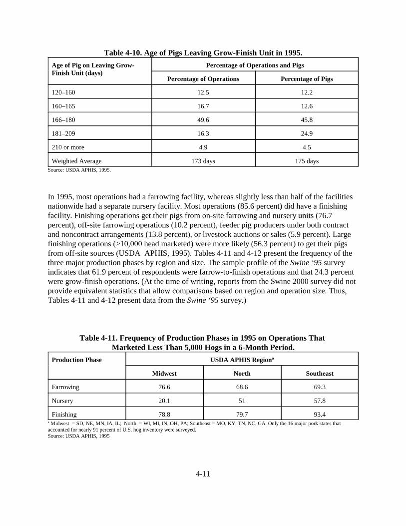
4-11

Table 4-10. Age of Pigs Leaving Grow-Finish Unit in 1995.

Age of Pig on Leaving Grow-Finish Unit (days)

Percentage of Operations and Pigs

Percentage of Operations Percentage of Pigs

120–160 12.5 12.2

160–165 16.7 12.6

166–180 49.6 45.8

181–209 16.3 24.9

210 or more 4.9 4.5

Weighted Average 173 days 175 daysSource: USDA APHIS, 1995.

In 1995, most operations had a farrowing facility, whereas slightly less than half of the facilitiesnationwide had a separate nursery facility. Most operations (85.6 percent) did have a finishingfacility. Finishing operations get their pigs from on-site farrowing and nursery units (76.7percent), off-site farrowing operations (10.2 percent), feeder pig producers under both contractand noncontract arrangements (13.8 percent), or livestock auctions or sales (5.9 percent). Largefinishing operations (>10,000 head marketed) were more likely (56.3 percent) to get their pigsfrom off-site sources (USDA APHIS, 1995). Tables 4-11 and 4-12 present the frequency of thethree major production phases by region and size. The sample profile of the Swine ‘95 surveyindicates that 61.9 percent of respondents were farrow-to-finish operations and that 24.3 percentwere grow-finish operations. (At the time of writing, reports from the Swine 2000 survey did notprovide equivalent statistics that allow comparisons based on region and operation size. Thus,Tables 4-11 and 4-12 present data from the Swine ‘95 survey.)

Table 4-11. Frequency of Production Phases in 1995 on Operations That Marketed Less Than 5,000 Hogs in a 6-Month Period.

Production Phase USDA APHIS Regiona

Midwest North Southeast

Farrowing 76.6 68.6 69.3

Nursery 20.1 51 57.8

Finishing 78.8 79.7 93.4a Midwest = SD, NE, MN, IA, IL; North = WI, MI, IN, OH, PA; Southeast = MO, KY, TN, NC, GA. Only the 16 major pork states thataccounted for nearly 91 percent of U.S. hog inventory were surveyed.Source: USDA APHIS, 1995

4-12

Table 4-12. Frequency of Production Phases in 1995 on Operations That Marketed 5,000 or More Hogs in a 6-Month Period.

Production Phase USDA APHIS Regiona


Farrowing 44.8 80.4 89

Nursery 75 67.1 97.4

Finishing 45.8 69.7 62.8a Midwest = SD, NE, MN, IA, IL; North = WI, MI, IN, OH, PA; Southeast = MO, KY, TN, NC, GA. Only the 16 major pork states thataccounted for nearly 91 percent of U.S. hog inventory were surveyed.Source: USDA APHIS, 1995.

Although many large operations continue to have the full range of production phases at onefacility, these operations are no longer the norm. More frequently, in new operations, severalspecialized farms are linked, or horizontally integrated, into a chain of production and marketing.Pigs begin in sowherds on one site, move to a nursery on another, and then move again to afinishing facility. Specialized operations can take advantage of skilled labor, expertise, advancedtechnology, streamlined management, and modern housing. However, the primary advantage ofspecialization is disease control. In a farrow-to-finish operation, a disease outbreak that begins inone phase of the operation can spread to the other phases. Physically separating the phases makesit easier to break this disease cycle. At the same time, separating phases spreads the cost ofestablishing swine operations, particularly if the different operations are owned by differentpersons.

Thus other categories of swine operations may comprise two or three of the three phrasesdescribed: combined farrow-nursery operations, which breed pigs and sell them at 40 to 60pounds to finishing operations; wean-to-finish operations, which finish weaned pigs; and farrow-to-finish operations, which handle all phases of production from breeding through finishing. Theemerging trend in the mid to late ‘90s was to produce pigs in two production phases rather thanin three. In two-phase production, the weaned pigs may go straight into the grower building orfinishing building, bypassing the nursery. The advantages of such practices are reducedtransportation costs, lessened animal stress, and reduced animal mortality.

4.1.3 Swine Facility Types and Management

Table 4-13 summarizes the five major housing configurations used by domestic swine producers.

Although there are still many operations at which pigs are raised outdoors, the trend in the swineindustry is toward larger confinement facilities where pigs are raised indoors. A typicalconfinement farrowing operation houses 3,000 sows, although some farrowing operations houseas many as 10,000 sows at one location, and farms are being planned that will house as many as

4-13

15,000 sows at one location. Typical nursery operations are much smaller with a capacity of onlyabout 1,500 head, but as stated earlier, separate nursery facilities are relatively uncommon.

Table 4-13. Summary of Major Swine Housing Facilities.

Facility Typea Description Applicability

Total confinement Pigs are raised in pens or stalls in an environmentally controlledbuilding.

Most commonly used in nurseryand farrowing operations and allphases of very large operations.Particularly common in theSoutheast.

Open building with no outsideaccess

Pigs are raised in pens or stalls butare exposed to natural climateconditions.

Relatively uncommon but used byoperations of all sizes.

Open building with outside access Pigs are raised in pens or stalls butmay be moved to outdoors.

Relatively uncommon, but used bysome small to mid-sized operations.

Lot with hut or no building Pigs are raised on cement or soil lotand are not confined to pens orstalls.

Used by small to mid-sizedoperations.

Pasture with hut or no building Pigs are raised on natural pastureland and are not confined to pens orstalls.

Traditional method of raising hogscurrently used only at smalloperations.

a These are the main facility configurations contained in the Swine ’95 Survey conducted by USDA APHIS, 1995.

The economic advantages of confined facilities have been the primary driving factor (especiallyat large operations) for farmers to abandon dry lot or pasture raising of hogs. Althoughcontrolled-environment buildings require a greater initial capital investment than traditional farmoperations, labor costs per unit output are significantly reduced. Furthermore, these facilitiesallow for far greater control of the production process, protect both animals and workers fromweather, and usually result in faster growth-to-market weight and better feed efficiency. Mostcontrolled-environment facilities employ “all in, all out” production, in which pigs are moved ingroups, and buildings are cleaned and disinfected between groups. It should be noted that thesuccess of a controlled-environment operation is highly dependent on properly functioningventilation, heating and cooling, and waste removal systems. A prolonged breakdown of any ofthese systems during extreme weather conditions can be catastrophic to the pig herd andeconomically devastating to the operator.

Facility requirements differ somewhat for each phase in a hog’s life cycle, and hence farrowing,nursery, and growing-finishing facilities are configured differently. For example, farrowingoperations require more intense management to ensure optimal production and reduce pigletmortality. A typical farrowing pen measures 5 by 7 feet, and the litter is provided with aprotected area of approximately 8 square feet. The sow is relegated to a section of the pen and isseparated from the piglets by low guard rails that reduce crushing but do not interfere with

4-14

suckling. Floors are usually slatted under or to the rear of the sow area to facilitate waste removal(NPPC, 1996).

Newly born piglets require special care because of their vulnerability to injury and disease.Nursery systems are typically designed to provide a warm, dry, and draft-free environment inwhich animal stress is minimized to promote rapid growth and reduce injury and mortality.Nursery rooms are regularly cleaned and sanitized to reduce the piglets’ exposure to pathogens.Nursery buildings are cleaned and disinfected thoroughly between groups of pigs to prevent thetransmission of disease from one herd to another. Nursery pens usually hold 10 to 20 pigs. Pigsare held in the nursery from weaning until they are 8 to 12 weeks old (NPPC, 1996).

Finishing pigs at tend to require less intensive management than piglets and can tolerate greatervariations in environmental conditions without incurring health problems. In an environmentallycontrolled building, growing and finishing pens hold 15 to 40 pigs and allow about 6 square feetper pig. Overcrowding leads to stress and aggressive behavior and can result in reduced growthrates and injury. Slatted concrete floors are the most common (NPPC, 1996).

Smaller facilities tend to use open buildings, with or without access to the outside. Usually, hogsraised in these buildings are also confined to pens or stalls. Depending on the climate, thebuilding might require ventilation and mist sprayer systems to prevent heat stress in the summer.Bedding might be needed during the winter months to protect the animals from the cold.

Hogs raised on dry lots or pasture require care and management similar to that for animals raisedindoors, plus additional measures to protect the herds from extreme weather conditions. Theymust be provided with sufficient shade to reduce heat stress in the summer. Where natural shadeis not available, facilities can be constructed to protect the herd from the sun in the summer andfrom wind and cold during the winter. Windbreaks are used under certain environmentalconditions.

The most comprehensive information on swine facility and waste management systems currentlyin use by farm type, size, and state location was collected in conjunction with USDA’s Swine ‘95study (USDA APHIS, 1995). Included in the study were 16 major pork-producing states thataccounted for almost 91 percent of the U.S. hog inventory and more than 70 percent of the porkproducers. The samples for the major swine-raising operations were statistically designed toprovide inferences to the nation’s swine population. Although the survey was conducted byAPHIS and focused on swine health issues, it contains information on swine production andfacility and waste management. Tables 4-14 and 4-15 present information on the housing typesused in the farrowing phase. Tables 4-16 and 4-17 present information on the housing types usedin the nursery phase. Tables 4-18 and 4-19 present information on the housing types used in thefinisher phase. These tables clearly demonstrate that the larger facilities tend to use totalconfinement in all regions. (At the time of writing, reports from the Swine 2000 survey did notprovide equivalent statistics that allow comparisons based on region and operation size. ThusTables 4-14 through 4-19 present data from the Swine ‘95 survey.)

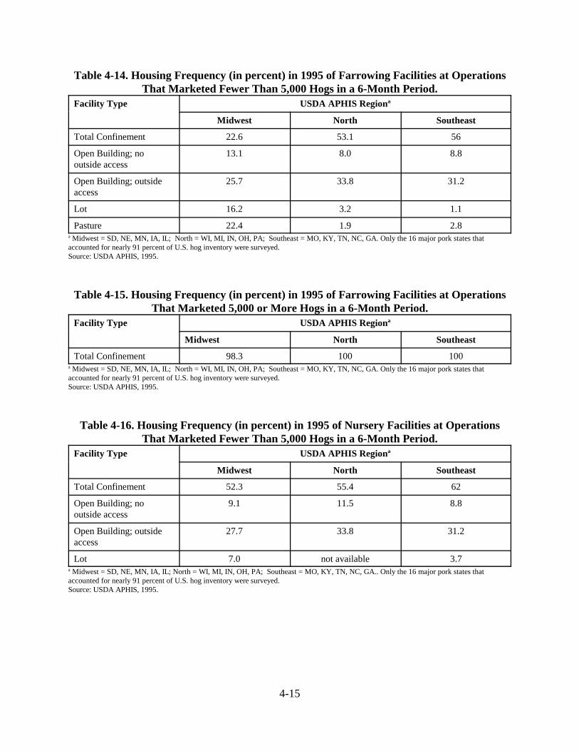
4-15

Table 4-14. Housing Frequency (in percent) in 1995 of Farrowing Facilities at OperationsThat Marketed Fewer Than 5,000 Hogs in a 6-Month Period.

Facility Type USDA APHIS Regiona


Total Confinement 22.6 53.1 56

Open Building; nooutside access

13.1 8.0 8.8

Open Building; outsideaccess

25.7 33.8 31.2

Lot 16.2 3.2 1.1

Pasture 22.4 1.9 2.8a Midwest = SD, NE, MN, IA, IL; North = WI, MI, IN, OH, PA; Southeast = MO, KY, TN, NC, GA. Only the 16 major pork states thataccounted for nearly 91 percent of U.S. hog inventory were surveyed.Source: USDA APHIS, 1995.

Table 4-15. Housing Frequency (in percent) in 1995 of Farrowing Facilities at OperationsThat Marketed 5,000 or More Hogs in a 6-Month Period.



Total Confinement 98.3 100 100a Midwest = SD, NE, MN, IA, IL; North = WI, MI, IN, OH, PA; Southeast = MO, KY, TN, NC, GA. Only the 16 major pork states thataccounted for nearly 91 percent of U.S. hog inventory were surveyed.Source: USDA APHIS, 1995.

Table 4-16. Housing Frequency (in percent) in 1995 of Nursery Facilities at OperationsThat Marketed Fewer Than 5,000 Hogs in a 6-Month Period.



Total Confinement 52.3 55.4 62


9.1 11.5 8.8


27.7 33.8 31.2

Lot 7.0 not available 3.7a Midwest = SD, NE, MN, IA, IL; North = WI, MI, IN, OH, PA; Southeast = MO, KY, TN, NC, GA.. Only the 16 major pork states thataccounted for nearly 91 percent of U.S. hog inventory were surveyed.Source: USDA APHIS, 1995.

4-16

Table 4-17. Housing Frequency (in percent) in 1995 of Nursery Facilities at OperationsThat Marketed 5,000 or More Hogs in a 6-Month Period.



Total Confinement 99 100 96.4a Midwest = SD, NE, MN, IA, IL; North = WI, MI, IN, OH, PA; Southeast = MO, KY, TN, NC, GA; Only the 16 major pork states thataccounted for nearly 91 percent of U.S. hog inventory were surveyed.Source: USDA APHIS, 1995.

Table 4-18. Housing Frequency (in percent) in 1995 of Finishing Facilities at OperationsThat Marketed Fewer Than 5,000 Hogs in a 6–Month Period



Total Confinement 19.9 36.5 23.4


15.4 14.1 9.5


24.5 42.1 55.9

Lot 17.1 4.6 9.3

Pasture 23.0 2.5 1.9a Midwest = SD, NE, MN, IA, IL; North = WI, MI, IN, OH, PA; Southeast = MO, KY, TN, NC, GA. Only the 16 major pork states thataccounted for nearly 91 percent of U.S. hog inventory were surveyed.Source: USDA APHIS, 1995.

Table 4-19. Housing Frequency (in percent) in 1995 of Finishing Facilities at OperationsThat Marketed 5,000 or More Hogs in a 6-Month Period.

VariableRegiona


Total Confinement 96.8 95.5 83.9a Midwest = SD, NE, MN, IA, IL; North = WI, MI, IN, OH, PA; Southeast = MO, KY, TN, NC, GA. Only the 16 major pork states thataccounted for nearly 91 percent of U.S. hog inventory were surveyed.Source: USDA APHIS, 1995.

4.1.4 Swine Waste Management Practices

Removal of manure from the animals’ living space is critical for animal and farm worker well-being. Odor, gases, and dust carried by ventilation exhaust air are also affected by the wastemanagement system used. Swine waste management systems can be separated into collection,storage, and treatment practices. An overview of the major practices in each of these areas ispresented below, and more detailed information on waste collection, storage, and treatmentpractices is provided in Section 8 of this document. Although the practices described below do

4-17

not represent all of the waste management practices in use today, they are the predominantpractices currently used at swine operations.

4.1.4.1 Swine Waste Collection Practices

Indoor raising of hogs requires that animals be physically separated from their waste products.Separation in larger facilities is usually accomplished through the use of concrete flooring withslots that allow the waste to drop below the living area and be transferred to a pit or troughbeneath the pen. Smaller facilities hand clean pens to collect wastes.

The most frequently reported waste management system used in 1990 was hand cleaning (41.6percent), which declined in use to 28.3 percent of operations in 1995 (USDA APHIS, 1995).This decrease in hand cleaning is highly correlated to the decrease in smaller facilities. Somefacilities separate solid material from liquids before moving the material to storage. (Adiscussion of solid-liquid separation is presented in Section 8.) Slatted floors are now morecommonly used to separate the manure from the animals at larger facilities. The waste is thendeposited in an under-floor pit or gutter where it is stored or moved to another type of storage.There are two main types of under-floor collection practices in which the waste is moved forstorage elsewhere.

• Pit recharge. Pit recharge is the periodic draining of the pit contents by gravity tostorage, followed by recharging the pit with new or recycled water. Regular pit drainingremoves much of the manure solids that would otherwise settle and remain in thebottom of the pit. The regular dissolution of settled solids increases the likelihood thesolids will be removed at the next pit draining. Recharge systems use a 16- to 18-inch-deep, in-house pit with 6 to 8 inches of water, which is emptied every 7 days to ananaerobic lagoon. Previously, 24-inch-deep pits were preferred, but now shallower pitsare used with the hog slat system.

• Flush. Flush systems may use fresh water or recycled lagoon water for frequent removalof feces and urine from under-floor collection gutters or shallow pits. Like pit rechargesystems, flush systems also improve animal health and performance as well as humanworking conditions in the swine houses by avoiding prolonged storage. Flush tanks withthe capacity to release at least 1.5 gallons per 100 pounds of live animal weight perflush are placed at the end of the swine houses. Pit floors should be level from side toside, and wide pits should be divided into individual channels no wider than 4 to 5 feet.The floor slope for most flush systems is between 1 and 2 percent. Floors are flushed atleast 1 to 12 times per day; the flush tanks are filled with new or recycled lagoon waterbefore every flush. The flushed waste is collected and removed from the houses intostorage through a system similar to that used in pit recharge systems.

4.1.4.2 Swine Waste Storage Practices

Waste storage is critical to the proper management of wastes from AFOs because manurenutrients are best applied to farmland only at certain times of the year, as determined by crops,climate, and weather. Storage practices include deep pits, anaerobic and aerobic lagoons, above

4-18

and belowground slurry storage (tanks or pits), and dry storage. Most large hog farms (more than80 percent) have from 90 to 365 days of waste storage capacity (see Table 4-20).

Table 4-20. Percentage of Swine Facilities With Manure Storage in 1998.Annual

Marketed Head0–3 months 3–6 months 6–9 months 9–12 months None or NA

NR 3.2 3.7 3.2 7.4 82.5

0-1,000 31.9 27.2 12.3 17.4 11.3

1,000-2,000 14.9 38.0 20.7 19.4 7.1

2,000-3,000 10.1 35.4 21.9 28.1 4.4

3,000-5,000 5.8 33.5 22.8 32.6 5.3

5,000-10,000 6.1 2 22.1 35.6 7.0

10,000-20,000 4.7 26.4 21.1 40.9 6.8

20,000-50,000 6.0 23.5 22.8 39.2 8.6

50,000 + 4.0 19.5 28.7 28.0 19.8 NA = Not reported/available. Source: NPPC, 1998.

An overview of common waste storage practices is provided below; more detailed informationcan be found in Section 8 of this document.

• Deep pit manure storage. Many operations use pits that are 6- to 8-feet deep andprovide for up to 6 months of storage under the house. Commonly, slurry is removedfrom the pit twice a year. The slurry is disposed of through direct surface application orsubsurface injection, transferred to an earthen storage facility, or pumped to an above orbelowground storage tank. This slurry system produces a waste stream with higher drymatter content (4 to 5 percent) and higher nutrient content than other liquid manuresystems. The above and belowground storage systems conserve more N than othersystems (N loss of only 10 to 30 percent). Operations use this system to avoid problemsassociated with lagoons such as odor, ammonia volatilization, and ground water impactresulting from leaking lagoons.

• Lagoon Systems. Lagoon systems can serve as both storage and treatment units.Anaerobic lagoons are the most common type of lagoon and are characterized byanaerobic decomposition of organic wastes. When properly designed an anaerobiclagoon will have a minimum total capacity that includes appropriate design treatmentcapacity, additional storage for sludge accumulation, and temporary storage for rainfalland wastewater inputs. A lagoon should also have sufficient freeboard and an indicatorof the highest safe water level, to prevent the wastewater from overflowing theembankment.

• Lagoons usually fill to capacity within 2 to 3 years of startup due to the accumulatedwaste volume and, depending on the region, rainfall in excess of evaporation. When the

4-19

lagoon is full, water overflow will occur unless the operator is in a position to apply theexcess water to the land. Lagoon water drawdown by irrigation or other methods isusually begun before the water reaches the maximum wastewater storage level. Severalstates require that liquid level indicators be placed in the lagoon to be sure that theliquid stays below the level required to contain the 24-hour, 25-year storm.

In addition to anaerobic lagoons, there are aerobic lagoons (which mix and aerate wastevia mechanical aerators or ozone generators), two-stage lagoons (typically a constantvolume covered treatment cell followed by a storage cell), and multistage cell lagoons.Technical information and a discussion of the advantages and disadvantages of thesetypes of lagoons is presented in Section 8 of this document.

• Settling and evaporation ponds. Earthen ponds are used by some swine operations forsolids separation. These ponds are designed to remove 40 percent of the total solids (in a6 percent solids form) based on 3 months of storage. The material is then moved toanother earthen pit, which serves as a drying bed, or flow is diverted to a parallel solidsremoval pond. The slurry dries to about 38 percent solids and 3-inch thickness within 6months. The material is then moved with a front-end loader into a box-type spreader andapplied to the land. Solids drying ponds and beds are not covered and therefore exposedto rainfall. A floating pump is located half the lagoon distance from the inlet, with ascreen over the intake to protect sprinkler nozzles. The supernatant is pumped and usedto irrigate fields. Another variation is to use a single lagoon followed by an evaporationpond that is 6 feet deep and as big as possible. Some evaporation ponds dry up duringthe summer. Because of odor problems, there is a trend away from the earthen pond forsolids separation to either a single anaerobic lagoon or an anaerobic lagoon and anevaporation pond.

Waste runoff storage. The systems described above can also be associated withoperations that maintain hogs on an outside lot for at least part of the time. Suchoperations might also use housing similar to the systems described above, but allowoutside access for the animals. Dry lot areas may be paved or dirt, and manure is storedin piles that are created by tractor or scraping systems. Although controls might be inplace to contain manure from enclosed areas through use of a deep pit or lagoon, theyare not generally protective of the outside environment. Other typical runoff controlsinclude surface diversions to prevent rainwater from running onto the lot, or a crudesettling basin with a slotted overflow.

• Other. Other types of waste management practices currently used include above andbelowground tanks (possibly covered or aerated), and hoop housing/deep beddingsystems.

USDA APHIS (2001) performed a survey of swine operations with 100 or more pigs. The studyincluded 17 of the major pork-producing states that account for 94 percent of the U.S. piginventory. Data for that survey were collected from 2,328 operations. The report providedinformation on feed and waste management, health and productivity, animal management, andfacility management. In addition to this report, NAHMS also performed additional analyses forEPA that present the percent of sites where pit holding was the waste management system used

4-20

most by region and herd size for the farrowing and grow-finish phase (USDA APHIS, 2002a).Tables 4.21 and 4.22 indicate the percent of sites where pit holding was the waste managementsystem used most.

Table 4-21. Percent of Sites Where Pit Holding was the Waste Management System usedmost by Region and Herd Size for Farrowing Phase.

States Total Inventory (head)Total 750–2500 >2500 +

Minnesota, Wisconsin, Michigan, Pennsylvania 37.3 50.3 49.3Colorado, South Dakota, Nebraska, Kansas, Missouri 22.6 37.9 50.2Iowa, Illinois, Indiana, Ohio 40.9 65.0 63.2Texas, Oklahoma, Arkansas, North Carolina 16.0 14.4 23.9

Source: USDA APHIS, 2002a.

Table 4-22. Percent of Sites Where Pit Holding was the Waste Management System usedmost by Region and Herd Size for Grower-Finisher Phase.

States Total Inventory (head)Total 750–2500 >2500 +

Minnesota, Wisconsin, Michigan, Pennsylvania 59.9 77.5 83.3Colorado, South Dakota, Nebraska, Kansas, Missouri 33.6 55.3 39.3Iowa, Illinois, Indiana, Ohio 48.3 67.6 77.5Texas, Oklahoma, Arkansas, North Carolina 27.7 26.3 37.5

Source: USDA APHIS, 2002a.

4.1.4.3 Swine Waste Treatment Practices

Many types of technology are used to treat swine wastes. These technologies work in a variety ofways to reduce the N, COD, and the volatile solids content of waste; or to change the form of thewaste to make it more concentrated and thus easier to handle. The most common type oftreatment practice is the anaerobic lagoon.

• Lagoon treatment systems. Lagoons designed to treat waste can reduce organic contentand N by more than 50 percent (PADER, 1986). Anaerobic lagoons are generallypreferred over aerobic lagoons because of their greater ability to handle high organicload. Nonetheless, incomplete anaerobic decomposition of organic material can result inoffensive by-products, primarily hydrogen sulfide, ammonia, and intermediate organicacids, which can cause disagreeable odors. Therefore, proper design, size, andmanagement are necessary to operate an anaerobic lagoon successfully.

New lagoons are typically half filled with water before waste loading begins. Starting upduring warm weather and seeding with bottom sludge from a working lagoon speedsestablishment of a stable bacterial population. Proper lagoon maintenance and operationis absolutely necessary to ensure that lagoon liner integrity is not affected, that bermsand embankments are stable, and the required freeboard and rainfall storage areprovided.

4-21

Even when bacterial digestion is efficient, significant amounts of sludge accumulate inanaerobic lagoons. Although lagoons can be designed with enough storage to minimizethe frequency of bottom sludge removals, at some point sludge accumulation willgreatly diminish the treatment capacity of most lagoons. Without the proper treatmentvolume, anaerobic decomposition will be incomplete, and odors will usually becomemore pronounced. Inadequate maintenance of treatment volume is the single mostcommon reason for the failure of lagoon treatment systems. The method used mostfrequently to remove sludge entails vigorous mixing of sludge and lagoon water bymeans of an agitator/chopper pump or propeller agitator. The operation of theagitator/chopper must be continuously monitored to prevent damage to the liner berms,or embankments, which could result in contamination of surface or ground water. Thesludge mixture is then pumped through an irrigation system onto cropland.

Some lagoons are covered with a synthetic material. There can be multiple advantagesto covering a lagoon. A cover will prevent rainfall from entering the system, which canresult in additional disposal costs. Nitrogen volatilization is minimized, making thewaste a more balanced fertilizer and potentially saving expenses for the purchase of Nfertilizers. The EPA AgSTAR Program has demonstrated that biogas production andsubsequent electricity generation from covered lagoons and digesters can be costeffective, help control odor, and provide for more effective nutrient management.

• Digesters. Conventional aerobic digestion is frequently used to stabilize biosolids atsmall municipal and industrial facilities as well as at some AFOs. Waste is aerated forrelatively long periods of time to promote microbial growth. Substantial reductions intotal and volatile solids, BOD, COD and organic N as well as some reduction inpathogen densities can be realized. Autoheated aerobic digesters use the heat releasedduring digestion to increase reaction rates and allow for more rapid reduction ofpathogens. The biosolids created by digesters concentrate solids, resulting in easierhandling. Additional information on the operational considerations, performance, andadvantages and disadvantages of digesters can be found in Section 8.

• Sequencing batch reactors. Manure is treated in sequence, typically in a vessel of metalconstruction. The vessel is filled, reacted (aeration cycled on and off), and then allowedto settle. Organic carbon and ammonia are reduced and P is removed through biosolidsgeneration or chemical precipitation. The biosolids generated are in a concentratedform, allowing for ease in handling.

• Other. Many other practices are used separately or in combination with the practiceslisted above to treat swine wastes. Constructed wetland treatment cells, trickling filters,composting, oxidation ditches, are a few of the other ways to treat swine wastes.Systems being developed or under trial studies include Y- or V- shaped pits withscrapers for solid-liquid separation at the source, membrane filtration, chemicaltreatments, high-rise hog buildings, oligolysis, hydroponic cultivation, photosyntheticdigesters, and closed loop water use systems using ultraviolet disinfection. Informationon the operational considerations, performance, and advantages and disadvantages ofthese and other treatment practices can be found in Section 8.

4-22

4.1.4.4 Waste Management Practices by Operation Size and Geographical Location

The use of a particular waste management system is driven by the size of the operation and geographic considerations (e.g., climate). For example, operation of a confined facility with theuse of a lagoon for treatment requires substantial capital investment. Below a certain number ofhead, such a system would be cost-prohibitive since the high start-up and maintenance costs ofsuch a facility have to be spread over a large number of animals to ensure economic viability.Geographic considerations also play a role in waste management. Anaerobic lagoons arecommon in the Southeast, where factors such as land availability and climate conditions arefavorable. Midwestern farms are more likely to use pit storage with slurry transport to above orbelowground tanks. The Swine ’95 Survey (USDA APHIS, 1995) provides a detailed picture ofswine management practices by operation type, size, and location. (At the time of writing, reportsfrom the Swine 2000 survey did not provide equivalent statistics that allow comparisons basedon region and operation size and is therefore not presented in this section.)

Waste Management Practice by Operation Size

As mentioned previously, large operations (greater than 2,000 head marketed in the past 12months) are much more likely to use water for waste management than small operations. Smalloperations (less than 500 head) typically manage waste by hand cleaning or mechanicalscraper/tractor. They also use pit-holding and flushing systems because of their relatively lowerlabor requirements. While larger operations also use pit storage and slurry storage in tanks, theyare far more likely to move waste from the housing facility to a lagoon. Tables 4-23, 4-24, and 4-25 present the frequency of operations using the most common types of waste managementsystems for swine farrowing, nursery, and finishing phases, respectively. Table 4-26 presents thefrequency of waste storage system use by size of operation. Table 4-27 presents the frequency ofwaste storage system use by region for operations that marketed 5,000 or more hogs in a 12-month period. It should be noted that the percentages do not add to 100 percent. This is becausean operation may use more than one waste storage system. For example, many large facilities inthe Southeast have below floor slurry storage that is then moved to lagoon storage.

Table 4-23. Frequency (in percent) of Operations in 1995 by Type of Waste ManagementSystem Used Most in the Farrowing Phase.

Variable

Number of Hogs Marketed in Past 12 Months

<2,000 2,000–10,000 >10,000

None 14.1 5.6 1.7

Pit-holding 24.4 53.9 49

Scraper/Tractor 12.3 3.6 6.0

Hand cleaned 39.7 0.6 0

Flush - under slats 4.6 20.8 39.3

Flush - gutter 3.0 2.7 2.6

Other 1.8 13 1.5Source: USDA APHIS, 1995.

4-23

Table 4-24. Frequency (in percent) of Operations in 1995 by Type of Waste ManagementSystem Used Most in the Nursery Phase.

Variable


<2,000 2,000–10,000 >10,000

None 4.4 3.3 0

Pit-holding 32.3 55 48


Hand cleaned 31.7 1.6 0



Other 2.3 15 6.8Source: USDA APHIS, 1995.

Table 4-25. Frequency (in percent) of Operations in 1995 by Type of Waste ManagementSystem Used Most in the Finishing Phase.

Variable


<2,000 2,000–10,000 >10,000

None 15.2 4.6 0

Pit-holding 22.1 53 45.3


Hand Cleaned 28.0 3.0 0



Other 4.0 5.5 7.4Source: USDA APHIS, 1995.

Table 4-26. Frequency (in percent) of Operations in 1995 That Used Any of the FollowingWaste Storage Systems by Size of Operation.

Waste Storage System

Percentage of Operations by Number of Head Marketed for Slaughter

<2,000 Head 2,000–10,000 Head >10,000 Head

Below-floor slurry 43.6 70.4 47.9

Aboveground slurry 4.1 10.3 8.3

Belowground slurry 17.3 25.6 26.8

Anaerobic lagoon with cover 2.2 0.5 2.0

Anaerobic lagoon without cover 17.4 29.2 81.8

Aerated lagoon 1.3 6.9 1.0

Oxidation ditch 2.9 0.1 0.0

Solids separated from liquids 4.1 5.9 4.7

Other 0.6 0.0 1.1Source: USDA APHIS, 1995.

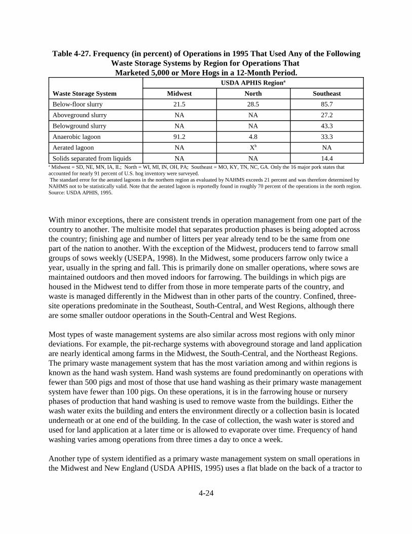
4-24

Table 4-27. Frequency (in percent) of Operations in 1995 That Used Any of the FollowingWaste Storage Systems by Region for Operations That

Marketed 5,000 or More Hogs in a 12-Month Period.

Waste Storage System

USDA APHIS Regiona


Below-floor slurry 21.5 28.5 85.7

Aboveground slurry NA NA 27.2

Belowground slurry NA NA 43.3

Anaerobic lagoon 91.2 4.8 33.3

Aerated lagoon NA Xb NA

Solids separated from liquids NA NA 14.4a Midwest = SD, NE, MN, IA, IL; North = WI, MI, IN, OH, PA; Southeast = MO, KY, TN, NC, GA. Only the 16 major pork states thataccounted for nearly 91 percent of U.S. hog inventory were surveyed. The standard error for the aerated lagoons in the northern region as evaluated by NAHMS exceeds 21 percent and was therefore determined byNAHMS not to be statistically valid. Note that the aerated lagoon is reportedly found in roughly 70 percent of the operations in the north region. Source: USDA APHIS, 1995.

With minor exceptions, there are consistent trends in operation management from one part of thecountry to another. The multisite model that separates production phases is being adopted acrossthe country; finishing age and number of litters per year already tend to be the same from onepart of the nation to another. With the exception of the Midwest, producers tend to farrow smallgroups of sows weekly (USEPA, 1998). In the Midwest, some producers farrow only twice ayear, usually in the spring and fall. This is primarily done on smaller operations, where sows aremaintained outdoors and then moved indoors for farrowing. The buildings in which pigs arehoused in the Midwest tend to differ from those in more temperate parts of the country, andwaste is managed differently in the Midwest than in other parts of the country. Confined, three-site operations predominate in the Southeast, South-Central, and West Regions, although thereare some smaller outdoor operations in the South-Central and West Regions.

Most types of waste management systems are also similar across most regions with only minordeviations. For example, the pit-recharge systems with aboveground storage and land applicationare nearly identical among farms in the Midwest, the South-Central, and the Northeast Regions.The primary waste management system that has the most variation among and within regions isknown as the hand wash system. Hand wash systems are found predominantly on operations withfewer than 500 pigs and most of those that use hand washing as their primary waste managementsystem have fewer than 100 pigs. On these operations, it is in the farrowing house or nurseryphases of production that hand washing is used to remove waste from the buildings. Either thewash water exits the building and enters the environment directly or a collection basin is locatedunderneath or at one end of the building. In the case of collection, the wash water is stored andused for land application at a later time or is allowed to evaporate over time. Frequency of handwashing varies among operations from three times a day to once a week.

Another type of system identified as a primary waste management system on small operations inthe Midwest and New England (USDA APHIS, 1995) uses a flat blade on the back of a tractor to

4-25

scrape or remove manure from feeding floors. The popularity of this system has apparentlywaned, and the it no longer represents a major means for removing wastes from swine feedingoperations (NCSU, 1998a).

Swine Waste Management Systems in the Pacific Region

Descriptive information about the waste management systems in this region is provided in Table4-28. In general, the region is characterized by operations with fewer than 500 pigs that use handwashing and dry lots as their primary waste management system. In contrast, the majority of pigsare raised on operations with more than 1,000 animals that use either deep pit/abovegroundstorage or pit recharge/lagoon.

Table 4-28. Distribution of Predominant Waste Management Systems in the Pacific Regiona in 1997.

Farm Size (number of pigs)Primary Waste

Management SystemFewer than 500 1. Hand Wash/Dry Lots

2. Scraper/Aboveground Storage/Land Application

500 to 1,000 1. Hand Wash/Dry Lots 2. Deep Pit/Aboveground Storage/Land Application

More than 1,000 1. Deep Pit/Aboveground Storage/Land Application2. Pit Recharge/Covered Anaerobic Lagoon/Irrigation

a Alaska, California, Hawaii, Oregon, and Washington.Source: NCSU, 1998a.

Swine Waste Management Systems in the Central Region

Table 4-29 presents information for the Central Region. It is the fastest-growing area of swineproduction in the nation at the present time. As a result, large operations (>2,000 head) accountfor almost all of the swine in these states. As a group, these large operations appear to rely onevaporation from lagoons, aeration of anaerobic lagoons, or biogas production from lagoons asthe main means for storing and treating swine waste.

Circle 4, one of the largest operations in the country, uses a pit-recharge system that is emptiedabout three times per week. Wastewater treatment is by a two-stage evaporative lagoon system.The primary stage is designed for treatment of volatile solids, with additional volume for 20years of sludge storage. The exact treatment volume design is operation- (or complex-) specificand takes into consideration the diet, feed digestibility, and absorption and conversion efficiencyof the animal for each group of confinement houses. The primary stage is sized on the basis ofvolume per input of volatile solids plus an additional volume for 20 years of sludge storage. Thesecondary stage lagoon volume and surface area are specified to allow evaporation of all excesswater not required for pit recharge. Waste management plans call for sludge removal every 20years. Because the operation has not reached its design life at this time, this system cannot beevaluated.

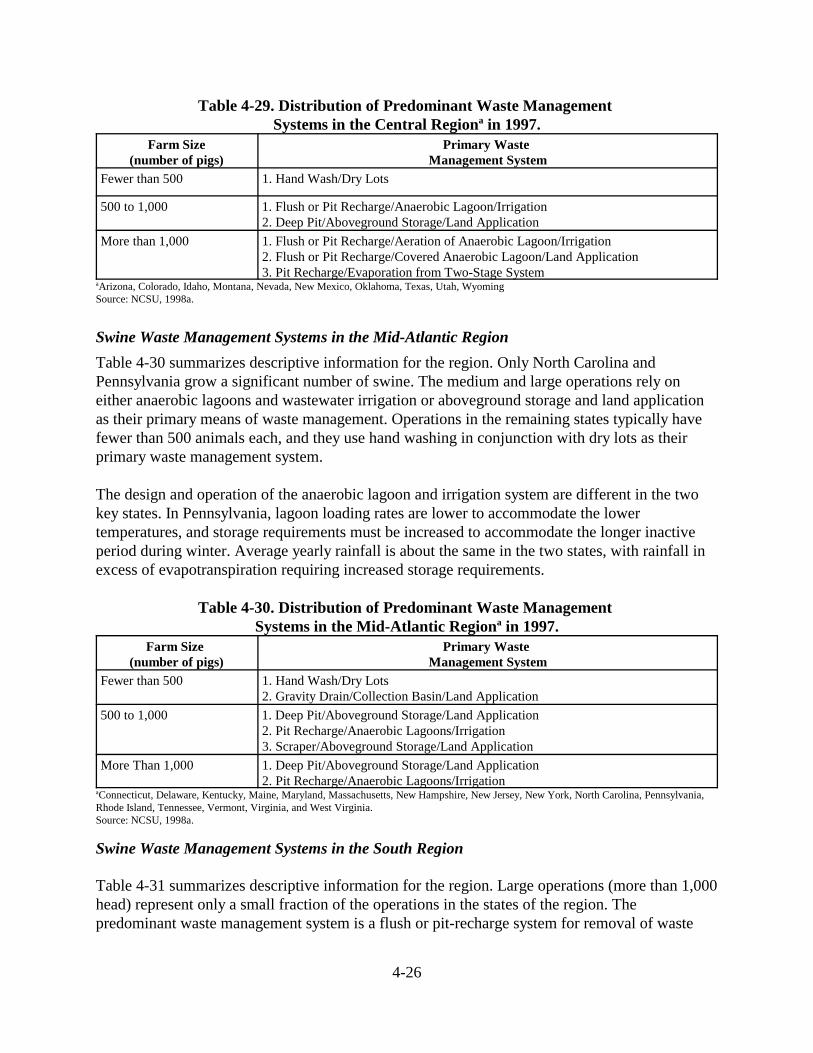
4-26

Table 4-29. Distribution of Predominant Waste Management Systems in the Central Regiona in 1997.

Farm Size(number of pigs)

Primary Waste Management System

Fewer than 500 1. Hand Wash/Dry Lots

500 to 1,000 1. Flush or Pit Recharge/Anaerobic Lagoon/Irrigation2. Deep Pit/Aboveground Storage/Land Application

More than 1,000 1. Flush or Pit Recharge/Aeration of Anaerobic Lagoon/Irrigation2. Flush or Pit Recharge/Covered Anaerobic Lagoon/Land Application3. Pit Recharge/Evaporation from Two-Stage System

aArizona, Colorado, Idaho, Montana, Nevada, New Mexico, Oklahoma, Texas, Utah, WyomingSource: NCSU, 1998a.

Swine Waste Management Systems in the Mid-Atlantic Region

Table 4-30 summarizes descriptive information for the region. Only North Carolina andPennsylvania grow a significant number of swine. The medium and large operations rely oneither anaerobic lagoons and wastewater irrigation or aboveground storage and land applicationas their primary means of waste management. Operations in the remaining states typically havefewer than 500 animals each, and they use hand washing in conjunction with dry lots as theirprimary waste management system.

The design and operation of the anaerobic lagoon and irrigation system are different in the twokey states. In Pennsylvania, lagoon loading rates are lower to accommodate the lowertemperatures, and storage requirements must be increased to accommodate the longer inactiveperiod during winter. Average yearly rainfall is about the same in the two states, with rainfall inexcess of evapotranspiration requiring increased storage requirements.

Table 4-30. Distribution of Predominant Waste Management Systems in the Mid-Atlantic Regiona in 1997.

Farm Size (number of pigs)

Primary Waste Management System

Fewer than 500 1. Hand Wash/Dry Lots2. Gravity Drain/Collection Basin/Land Application

500 to 1,000 1. Deep Pit/Aboveground Storage/Land Application2. Pit Recharge/Anaerobic Lagoons/Irrigation3. Scraper/Aboveground Storage/Land Application

More Than 1,000 1. Deep Pit/Aboveground Storage/Land Application2. Pit Recharge/Anaerobic Lagoons/Irrigation

aConnecticut, Delaware, Kentucky, Maine, Maryland, Massachusetts, New Hampshire, New Jersey, New York, North Carolina, Pennsylvania,Rhode Island, Tennessee, Vermont, Virginia, and West Virginia.Source: NCSU, 1998a.

Swine Waste Management Systems in the South Region

Table 4-31 summarizes descriptive information for the region. Large operations (more than 1,000head) represent only a small fraction of the operations in the states of the region. Thepredominant waste management system is a flush or pit-recharge system for removal of waste

4-27

from buildings, an anaerobic lagoon for treatment and storage of waste, and reincorporation oftreated wastewater back into the environment by irrigation. In these states, housing is usuallyenclosed, with ventilation and a concrete floor surface.

Table 4-31. Distribution of Predominant Waste ManagementSystems in the South Regiona in 1997.

Farm Size (number of pigs) Primary Waste Management System

Fewer than 500 1. Hand Wash/Dry Lots2. Scraper System/ Aboveground Storage/Land Application

500 to 1,000 1. Flush or Pit Recharge/Anaerobic Lagoon/Irrigation

More Than 1,000 1. Flush or Pit Recharge/Anaerobic Lagoon/IrrigationaAlabama, Arkansas, Florida, Georgia, Kentucky, Louisiana, Mississippi, North Carolina, and South Carolina.Source: NCSU, 1998a.

Swine Waste Management Systems in the Midwest Region

Table 4-32 summarizes descriptive information for this region. Small operations account formost of the operations in this region; however, recent construction of large units in Iowa,Minnesota, Missouri, and South Dakota indicate that the trend toward production in larger unitsseen in the southeastern United States is probably occurring in the Midwest Region as well.Primary waste management systems for operations with fewer than 500 pigs are hand washcoupled with dry lots with and without collection basins. In contrast, medium and largeoperations rely on storage of waste either under buildings with deep pits or in abovegroundstructures in conjunction with direct land application for crop production.

Table 4-32. Distribution of Predominant Waste Management Systems in the Midwest Regiona in 1997.

Farm Size (number of pigs) Primary Waste Management System

Fewer than 500 1. Hand Wash/Dry Lots2. Hand Wash/Dry Lots and Collection Basin/Land Application3. Deep Pit/Land Application

500 to 1,000 1. Deep Pit/Aboveground Storage/Land Application2. Pit Recharge/Aeration of Anaerobic Lagoons/Irrigation 3. Deep Pit/Land Application

More than 1,000 1. Deep Pit/Aboveground Storage/Land Application2. Pit Recharge/Covered Anaerobic Lagoon/Irrigation

aIllinois, Indiana, Iowa, Kansas, Michigan, Minnesota, Missouri, Nebraska, North Dakota, Ohio, South Dakota, and Wisconsin.Source: NCSU, 1998a.

4-28

4.1.5 Pollution Reduction

4.1.5.1 Swine Feeding Strategies

Swine producers use a variety of feed ingredients to achieve a balanced diet for a pig at eachphase of the animal’s development. Various grain products, including corn, barley, milo, andsometimes wheat, form the foundation of the growing pig’s diet and supply most of thecarbohydrates and fat. Oilseed meals, which foster muscle and organ development, are theprimary source of protein (NPPC, 1999). Producers also supplement the basic diet with mineralsand vitamins as needed. A pig’s diet changes as the animal grows. For example, finishing pigstypically receive a diet containing 13 to 15 percent crude protein versus the 20 to 22 percentprotein diet received by young pigs. The Swine ’95 survey indicates that more than 96 percent ofgrow-finish operations use multiple diets from time of entry to market weight. Almost 70 percentof the operations feed their pigs three or more diets during this phase.

Swine operations can use feeding strategies both to maximize growth rates and to reduceexcretion of nutrients. The following feeding strategies can be used to reduce N and P manurecontent.

Grinding. Fine grinding and pelleting are simple but effective ways to improve feed utilizationand decrease N and P excretion. By reducing the particle size, the surface area of the grainparticles is increased, allowing for greater interaction with digestive enzymes. When particle sizeis reduced from 1,000 microns to 400 microns, N digestibility increases by approximately 5 to 6percent. As particle size is reduced from 1,000 microns to 700 microns, excretion of N is reducedby 24 percent. The current average particle size is approximately 1,100 microns; therecommended size is between 650 and 750 microns. Reducing particle size below 650 to 750microns greatly increases the energy costs of grinding and reduces the throughput of the mill. Theuse of so small a particle size will also increase the incidence of stomach ulcers in the hogs(NCSU, 1998b).

Amino Acid Supplemental Diets. Supplementing the diet with synthetic lysine to meet a portionof the dietary lysine requirement is an effective means of reducing N excretion by hogs. Thisprocess reduces N excretion because lower-protein diets can be fed when lysine is supplemented.Research studies have shown that protein levels can be reduced by 2 percent when the diet issupplemented with 0.15 percent lysine (3 pounds lysine-HC1/ton of feed) without negativelyaffecting the performance of grow-finish pigs. Greater reductions in protein are possible, but onlyif threonine, tryptophan, and methionine are also supplemented.

Table 4-33 shows the theoretical effect of feeding low-protein, amino acid-supplemented diets onN excretion of finishing pigs. Note that reducing the protein level from 14 to 12 percent andadding 0.15 percent lysine results in an estimated 22 percent reduction in N excretion. Reducingthe protein further to 10 percent and adding 0.30 percent lysine, along with adequate threonine,tryptophan, and methionine, reduces the estimated N excretion by 41 percent.

4-29

Although it is currently cost-effective to use supplemental lysine and methionine, supplementalthreonine and tryptophan are too expensive to use in widespread diets. However, because of rapidtechnological advances in fermentation procedures for synthesizing amino acids, the price ofthreonine and tryptophan will likely decrease in the next few years.

Table 4-33. Theoretical Effects of Reducing Dietary Protein and Supplementing WithAmino Acids on Nitrogen Excretion by 200-lb Finishing Piga,b

Diet Concentration 14 CP 12 CP + Lysine

10 CP + Lysine +Threonine + Tryptophan

+ MethionineN balance

N intake, g/d 67 58 50

N digested and absorbed, g/d 60 51 43

N excreted in feces, g/d 7 7 7

N retained, g/d 26 26 26

N excreted in urine, g/d 34 25 17

N excreted, total, g/d 41 32 24

Reduction in N excretion, % ---- 22 41

Change in dietary costs, $/tonb 0 -0.35 +$14.50aAssumes an intake of 6.6 lb/d and a growth rate of 1.98 lb/d. bCosts used L-Lysine HCl, $2.00/lb; corn, $2.50/bushel; SBM, $250/ton; L-Threonine, $3.50/lb; DL-Methionine, $1.65/lb; Tryptosine (70:15, Lys:Tryp) $4.70/lb.Source: NCSU, 1998b.g/d = grams/day

Phase Feeding and Split-Sex Feeding. Dividing the growth period into more phases with lessspread in weight allows producers to meet the pig’s protein requirements more closely. Also, since gilts (females) require more protein than barrows (males), penning barrows separately fromgilts allows lower protein levels to be fed to barrows without compromising leanness andperformance efficiency in gilts. Feeding three or four diets, compared with only two diets, duringthe grow-finish period would reduce N excretion by at least 5 to 8 percent (NCSU, 1998b).

Formulating Diets on an Available Phosphorus Basis. A high proportion (56 to 81 percent) ofthe P in cereal grains and oilseed meals occurs as phytate. Pigs do not use P in this form wellbecause they lack significant amounts of intestinal phytase, the enzyme needed to remove thephosphate groups from the phytate molecule. Therefore, supplemental P is added to the diet tomeet the pig’s growth requirements.

Because some feedstuffs are high in phytate and because there is some endogenous phytase incertain small grains (wheat, rye, triticale, and barley), there is wide variation in the bioavailabilityof P in feed ingredients. For example, only 12 percent of the total P in corn is available, whereas50 percent of the total P in wheat is available. The P in dehulled soybean meal is more availablethan the phosphorus in cottonseed meal (23 percent versus 1 percent), but neither source of P isas highly available as the P in meat and bone meal (66 percent), fish meal (93 percent), ordicalcium phosphate (100 percent) (NCSU, 1998b).

4-30

Supplementing Diets with Phytase Enzyme. Supplementing the diet with the enzyme phytaseis an effective means of increasing the breakdown of phytate P in the digestive tract and reducingthe P excretion in the feces. Using phytase allows one to feed a lower P diet because theunavailable phytate phosphorus in the grain and soybean meal is made available by the phytaseenzyme to help meet the pig’s P needs. Studies at Purdue University, the University of Kentucky,and in Denmark indicate that the inclusion of phytase increased the availability of P in a corn-soydiet threefold, from 15 percent to 45 percent.

A theoretical example of using phytase is presented in Table 4-34. If a finishing pig is fed a dietwith 0.4 percent P (the requirement estimated by NRC, 1988, cited in NCSU, 1998b), 12 gramsof P would be consumed daily (3,000 grams times 0.4 percent), 4.5 grams of P would beretained, and 7.5 grams of P would be excreted. Feeding a higher level of P (0.5, 0.6, or 0.7percent) results in a slight increase in P retention but causes considerably greater excretion of P(10.3, 13.2, and 16.2 g/d, respectively). Being able to reduce the P to 0.3 percent in a dietsupplemented with phytase would reduce the intake to 9 grams of P per day and wouldpotentially reduce the excreted P to 4.5 g/day (a 37 percent reduction in P excretion versusNRC’s estimate). The percent reduction in excreted P is even more dramatic (56 percent) whenone compares the 4.5 grams with the 10.3 grams of P excreted daily by finishing pigs fed at the0.5 percent P level typically recommended by universities and feed companies. Bone strength canbe completely recovered by supplementing a low-P diet with 1,000 phytase units per kilogramsof feed, while most of the grain and feed efficiency is returned to NRC levels. In addition toreturning bone strength and growth performance to control levels, there is a 32 percent reductionin P excretion. A summary of 11 experiments (Table 4-35) indicates that all the growth rate andfeed efficiency can be recovered with the dietary supplementation of 500 phytase units andreduced-P diets. Some analyses have suggested that a 50 percent reduction in excreted P by pigswould mean that land requirements for manure applications based on P crop uptake would becomparable to manure applications based on N.

Previously, phytase was too expensive to use as a feed additive. However, this enzyme can nowbe effectively produced by recombinant DNA techniques and the cost has decreased. A costevaluation indicates that under certain conditions replacing dietary P of an inorganic P source(e.g., dicalcium phosphate) with the phytase enzyme would be cost neutral. Swine require thatphytase supplements be fed at different levels based on the age of the pig (Table 4-36). The

Table 4-34. Theoretical Effects of Dietary Phosphorus Level and Phytase Supplementation (200-lb Pig).

Dietary P (%)Phosphorus (g/d) Change From Industry

Average (%)Intake Retained Excreted0.70 21.0 4.8 16.2 +570.60 18.0 4.8 13.2 +320.50 15.0 4.7 10.3 00.40 (NRC, 1988) 12.0 4.5 7.5 -270.30 9.0 2.5 6.5 -370.30 + Phytase 9.0 4.5 4.5 -56

Source: Cromwell and Coffey, 1995, cited in NCSU, 1998b.

4-31

Table 4-35. Effect of Microbial Phytase on Relative Performance of Pigs.a

Growth Response Negative Control Positive ControlEffect of 500+ Phytase

Units/kgADG 100 115 (+/- 6.5) 116.7 (+/ -10.6)

ADFI 100 105 (+/- 5.2) 107.6 (+/- 7.8)

Feed Conversion Ratio 100 93 (+/- 4.9) 93.2 (+/- 5.0)aEleven experiments with the negative control diets set at 100 percent and the relative change in pig growth performance to the control diets.Source: Jongbloed et al., 1996, cited in NCSU, 1998b.

Table 4-36. Effect of Microbial Phytase on Increase in Phosphorus Digestibility by Age ofPigs and the Recommended Rates for Inclusion of Phytase in Each Phase.

Nursery Grower Finisher Gestation LactationApproximateIncrease (%)

13 17 17 7 20

Inclusion Level(Phytase Unit/lb)

454–385 385–227 27–113 227 227

Source: Jonbloed et al., 1996, cited in NCSU, 1998b.

different levels are based on phase of production and are likely related to the digestive enzymesand cecum of the younger pig being less developed.

4.1.5.2 Waste and Waste Water Reductions

Methods to reduce the quantity of wastewater generated at swine operations include advancedswine watering systems to reduce water spillage and recycling water in waste flush systems. Thefeeding strategies discussed in the previous section will also reduce the quantity of wastegenerated by ensuring that animals do not receive more feed than required for optimal growth.Additional information on feeding strategies for swine can be found in Chapter 8. Advancedswine breeding has resulted in animals that produce less waste per pound of meat produced.

Nipple water delivery systems reduce the amount of wastewater and are more healthy for theanimals. Trough or cup waters are typically placed close to the floor of the pen. This allows theanimal to spill water and add contaminates to the standing water. Nipple water delivery systemsare placed higher in the pen and only deliver water to the animal when the animal is sucking onthe nipple. Watering systems may also use water pressure sensors and automatic shutoff valves toreduce water spillage. The sensor will detect a sustained drop in water pressure resulting from abreak in the water line. The sensor will then stop the water flow to the broken line and an alarmwill sound. The operator can then fix the broken line and restore water to the animals withminimal water spillage. There is little information about the relative use of the various waterdelivery systems or the relative use of water pressure sensors and shutoff valves within the swineindustry.

The use of recycled water in swine flush and pull plug waste management systems will alsoreduce the amount of wastewater generated at an operation. To obtain recycled water of

4-32

appropriate quality an operation can use a variety of methods to remove pollutants from thewaste stream. Such methods include solid-liquid separation, digesters, and multiple-stage lagoonsystems. Multiple-stage lagoon systems or the use of an initial settling basin will allow settling ofsolids and biological processes to occur that can result in high quality water. One large operationin Utah claims to have a completely closed system in which all wastewater is treated in amultiple-stage lagoon system and then recycled back to the manure flush system.

4.1.6 Waste Disposal

Waste is disposed in either a liquid or solid form. Handling and disposal in a solid form hasseveral advantages the more concentrated the waste. Hauling costs are reduced as the watercontent is reduced; however, most operations prefer to handle and dispose of waste in a liquidform because of the reduced labor cost of handling the waste in this manner. Table 4-37 showsthe percentage of operations that use or dispose of manure and wastes as unseparated liquids andsolids. Tables 4-38 and 4-39 show the percentage of operations that are using the most commondisposal methods by USDA APHIS region. (At the time of writing, reports from the Swine 2000survey did not provide equivalent statistics that allow comparisons based on region and operationsize and is therefore not presented in this section.)

Table 4-37. Percentage of Operations in 1995 That Used or Disposed of Manure and Wastes as Unseparated Liquids and Solids.

Operation Size

USDA APHIS Regiona


Operations marketing fewer than 5,000hogs in 12 months

92.3 99.1 97.7

Operations marketing 5,000 or morehogs in 12 months

100 19.6b 98.5

aMidwest = SD, NE, MN, IA, IL; North=WI, MI, IN, OH, PA; Southeast = MO, KY, TN, NC, GA. Only the 16 major pork states that accountedfor nearly 91 percent of U.S. hog inventory were surveyed. bThe standard error on this measurement is 16.0, resulting in questions of its accuracy.Source: USDA NAHMS, 1999.

Table 4-38. Percentage of Operations in 1995 That Marketed Fewer Than 5,000 Hogs in a12-Month Period and That Used the Following Methods of Use/Disposal by Region.

Waste Disposal Method

USDA APHIS Regiona


Placed on own land 97.9 98.5 96.8

Given away NA 11.0 2.6aMidwest=SD, NE, MN, IA, IL; North=WI, MI, IN, OH, PA; Southeast=MO, KY, TN, NC, GA. Only the 16 major pork states that accountedfor nearly 91 percent of U.S. hog inventory were surveyed. Source: USDA NAHMS, 1999.

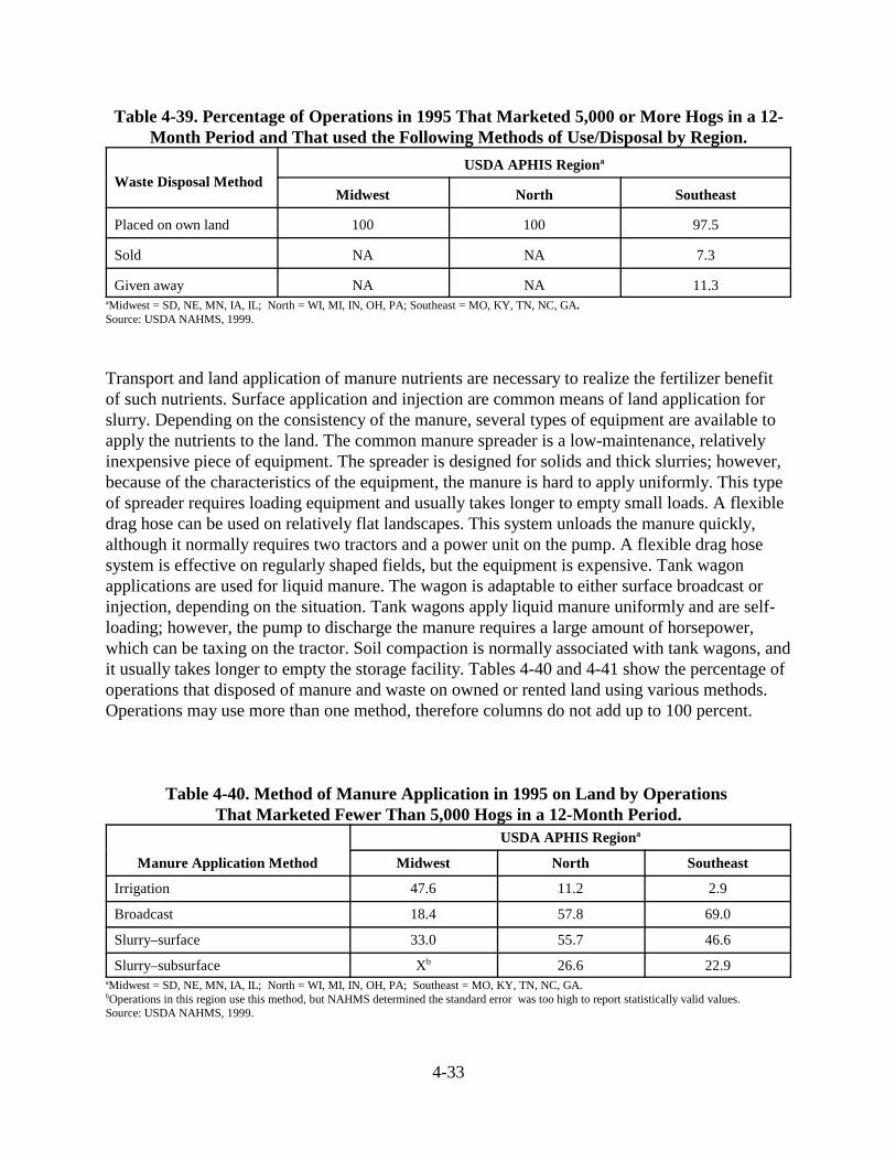
4-33

Table 4-39. Percentage of Operations in 1995 That Marketed 5,000 or More Hogs in a 12-Month Period and That used the Following Methods of Use/Disposal by Region.

Waste Disposal MethodUSDA APHIS Regiona


Placed on own land 100 100 97.5

Sold NA NA 7.3

Given away NA NA 11.3aMidwest = SD, NE, MN, IA, IL; North = WI, MI, IN, OH, PA; Southeast = MO, KY, TN, NC, GA.Source: USDA NAHMS, 1999.

Transport and land application of manure nutrients are necessary to realize the fertilizer benefitof such nutrients. Surface application and injection are common means of land application forslurry. Depending on the consistency of the manure, several types of equipment are available toapply the nutrients to the land. The common manure spreader is a low-maintenance, relativelyinexpensive piece of equipment. The spreader is designed for solids and thick slurries; however,because of the characteristics of the equipment, the manure is hard to apply uniformly. This typeof spreader requires loading equipment and usually takes longer to empty small loads. A flexibledrag hose can be used on relatively flat landscapes. This system unloads the manure quickly,although it normally requires two tractors and a power unit on the pump. A flexible drag hosesystem is effective on regularly shaped fields, but the equipment is expensive. Tank wagonapplications are used for liquid manure. The wagon is adaptable to either surface broadcast orinjection, depending on the situation. Tank wagons apply liquid manure uniformly and are self-loading; however, the pump to discharge the manure requires a large amount of horsepower,which can be taxing on the tractor. Soil compaction is normally associated with tank wagons, andit usually takes longer to empty the storage facility. Tables 4-40 and 4-41 show the percentage ofoperations that disposed of manure and waste on owned or rented land using various methods.Operations may use more than one method, therefore columns do not add up to 100 percent.

Table 4-40. Method of Manure Application in 1995 on Land by Operations That Marketed Fewer Than 5,000 Hogs in a 12-Month Period.

Manure Application Method

USDA APHIS Regiona


Irrigation 47.6 11.2 2.9

Broadcast 18.4 57.8 69.0

Slurry–surface 33.0 55.7 46.6

Slurry–subsurface Xb 26.6 22.9aMidwest = SD, NE, MN, IA, IL; North = WI, MI, IN, OH, PA; Southeast = MO, KY, TN, NC, GA.bOperations in this region use this method, but NAHMS determined the standard error was too high to report statistically valid values.Source: USDA NAHMS, 1999.

4-34

Table 4-41. Method of Manure Application in 1995 on Land by Operations That Marketed 5,000 or More Hogs in 12-Month Period.

Manure Application Method

USDA APHIS Regiona


Irrigation 100 74.8 16.4

Broadcast Xb Xb 39.4

Slurry–surface Xb 6.3 68.1

Slurry–subsurface Xb 23.6 72.1 Midwest = SD, NE, MN, IA, IL; North = WI, MI, IN, OH, PA; Southeast = MO, KY, TN, NC, GA.bOperations in this region use this method, but NAHMS determined the standard error was too high to report statistically valid values. Source: USDA NAHMS, 1999.

Most manure and waste is disposed of on land owned or rented by the operator, thus the amountof land available for land application of wastes is critical. Applying too much manure and wasteto the same land year after year can result in a steady increase in the soil P content. Table 4-8presents the number of swine operations with and without adequate crop and pastureland formanure application on an N- and P- basis at plant removal rates and operations that own no land.The operations that have no land were determined by running queries of the USDA 1997 Censusof Agriculture data to identify facilities that did not grow any of the 24 major crops grown in theUnited States. Operations with no land available are assumed to haul their waste to land that canuse the waste as a fertilizer resource.

Another waste product of swine farms is animal mortality. Mortalities are usually handled in anenvironmentally sound and responsible manner, but improper disposal may cause problems withodors, pathogens, biosecurity, and soil and water contamination. The 1995 USDA APHIS Swine95 study assessed the frequency of mortality disposal methods based on whether operationsmarketed more or fewer than 2,500 head in the prior 6 month period. (An operation that sold2,500 head in the last 6 months corresponds roughly to an operation with 1,000 to 1,500 animalunit capacity.) Tables 4-42 and 4-43 show the percentage of operations by method of disposalfor those operations which specified at least one pig had died in the 6 month period.

Table 4-42. Method of Mortality Disposal on Operations That Marketed Fewer Than 2,500 Hogs in a 6-Month Period in 1995.

Method of disposal

USDA APHIS Regiona


Burial on operation 73.2 71.6 46.6

Burn on operation 9.1 7.2 15.2

Renderer entering operation 2.1 14.1 38.7

Renderer at perimeter of operation 2.7 4.2 8.7

Composting 10.3 6.4 13.0

Other 7.0 9.8 6.8aMidwest = SD, NE, MN, IA, IL; North = WI, MI, IN, OH, PA; Southeast = MO, KY, TN, NC, GA. Only the 16 major pork states thataccounted for nearly 91 percent of U.S. hog inventory were surveyed. Source: USDA NAHMS, 1999.

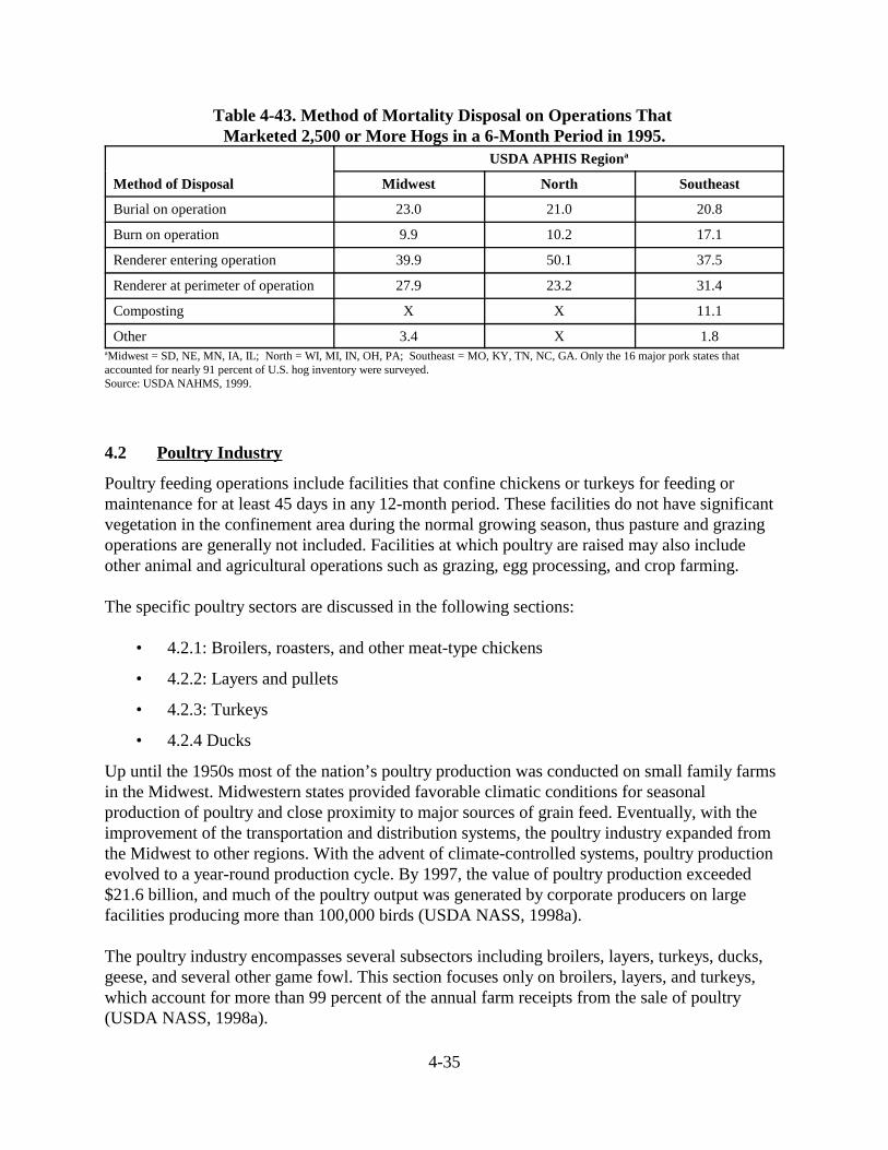
4-35

Table 4-43. Method of Mortality Disposal on Operations That Marketed 2,500 or More Hogs in a 6-Month Period in 1995.

Method of Disposal

USDA APHIS Regiona


Burial on operation 23.0 21.0 20.8

Burn on operation 9.9 10.2 17.1

Renderer entering operation 39.9 50.1 37.5

Renderer at perimeter of operation 27.9 23.2 31.4

Composting X X 11.1

Other 3.4 X 1.8aMidwest = SD, NE, MN, IA, IL; North = WI, MI, IN, OH, PA; Southeast = MO, KY, TN, NC, GA. Only the 16 major pork states thataccounted for nearly 91 percent of U.S. hog inventory were surveyed. Source: USDA NAHMS, 1999.

4.2 Poultry Industry

Poultry feeding operations include facilities that confine chickens or turkeys for feeding ormaintenance for at least 45 days in any 12-month period. These facilities do not have significantvegetation in the confinement area during the normal growing season, thus pasture and grazingoperations are generally not included. Facilities at which poultry are raised may also includeother animal and agricultural operations such as grazing, egg processing, and crop farming.

The specific poultry sectors are discussed in the following sections:

• 4.2.1: Broilers, roasters, and other meat-type chickens

• 4.2.2: Layers and pullets

• 4.2.3: Turkeys

• 4.2.4 Ducks

Up until the 1950s most of the nation’s poultry production was conducted on small family farmsin the Midwest. Midwestern states provided favorable climatic conditions for seasonalproduction of poultry and close proximity to major sources of grain feed. Eventually, with theimprovement of the transportation and distribution systems, the poultry industry expanded fromthe Midwest to other regions. With the advent of climate-controlled systems, poultry productionevolved to a year-round production cycle. By 1997, the value of poultry production exceeded$21.6 billion, and much of the poultry output was generated by corporate producers on largefacilities producing more than 100,000 birds (USDA NASS, 1998a).

The poultry industry encompasses several subsectors including broilers, layers, turkeys, ducks,geese, and several other game fowl. This section focuses only on broilers, layers, and turkeys,which account for more than 99 percent of the annual farm receipts from the sale of poultry(USDA NASS, 1998a).

4-36

Together the annual sales of broilers, chicken eggs, and turkeys generate almost 10 percent of thevalue of all farm commodities. Although each of the poultry subsectors has experiencedsignificant growth in output over the past two decades, broilers remain the dominant subsector,accounting for approximately 65 percent ($14.2 billion) of the $21.6 billion in poultry farm salesduring 1997. Sales of eggs and turkeys accounted for 21 percent ($4.5 billion) and 13 percent($2.9 billion), respectively. More than 15 million metric tons of poultry meat were produced inthe U.S. during that year (USDA NASS, 1998c).

Poultry production (especially broiler production) is a highly integrated industry, and as a result,management strategies at the facility level tend to be more similar than in other sectors of AFOs.Contract growing began in the South during the 1930s, and by the 1950s the contracts hadevolved to their current form. Thus, the integrated structure seen today was in place by the 1960s(Sawyer, 1971, cited in Aust, 1997). For example, more than 90 percent of all chickens raised forhuman consumption in the U.S. are produced by independent farmers working under contractwith integrated chicken production and processing companies. The company provides someinputs such as the birds themselves, feed, medication, and monitoring of flock health by companyservice personnel. The farmer provides the grow-out buildings, electricity, water, fuel, beddingmaterial (“litter”), and labor and management skills. The company provides the newly hatchedchicks that the farmer raises to market age and weight, giving them the feed provided by thecompany. The farmer is paid largely on the basis of weight gained by the flock as compared withother flocks produced during the same span of time. When the birds reach market weight, thecompany picks them up and takes them to processing plants, where they are processed into foodproducts. Most integrated companies are stand-alone chicken operations, although some alsoproduce turkeys.

The poultry industry has continued to evolve in terms of the type and number of birds itproduces. Genetically designed birds have been developed with the ability to mature quickly andreach market weight or lay eggs more rapidly. This has resulted in increased efficiency andoverall poultry production. Facilities that grow the birds have incorporated the latest automatedtechnology for the feed and watering systems as well as ventilation systems. The technologicaladvances have transformed poultry raising into a modern, mechanized industry.

4.2.1 Broiler Sector

This section describes the following aspect of the broiler industry:

• 4.2.1.1: Distribution of the broiler industry by size and region

• 4.2.1.2: Production cycles of broilers

• 4.2.1.3: Broiler facility types and management4.2.1.4: Broiler waste managementpractices

• 4.2.1.5: Pollution reduction

• 4.2.1.6: Waste disposal

4-37

National Overview

Domestic broiler production has followed the same trend as swine and other livestock industries.Production has shifted from geographically diverse, small, family-run operations to largeindustrial production facilities concentrated in a few states. The number of broiler operations wasquite stable between 1992 and 1997, with operations decreasing slightly from 23,949 broileroperations in 1992 to 23,937 operations in 1997, down less than 1 percent (USDA NASS,1999b). However, between 1982 and 1992, more than 6,000 broiler operations, or 20 percent ofthe industry’s producers, went out of business. As shown in Table 4-44, although the number ofoperations decreased over the past 20 years, total broiler production increased, with new largeoperations more than compensating for the small producers who have left the industry.

Table 4-44. Broiler Operations and Production in the United States 1982–1997.a

Year Operations Production

1982 30,100 3,516,095,408

1987 27,645 4,361,198,301

1992 23,949 5,427,532,921

1997 23,937 6,741,476,153aBroilers are young chickens of the meat-type breeds, raised for the purpose of meat production. Estimates cover a 12-month period (Dec. 1through Nov. 30) and exclude states with fewer than 500,000 broilers.Source: USDA NASS, 1998a, 1998b.

4.2.1.1 Distribution of Broiler Operations by Size and Region

EPA’s 1974 CAFO Effluent Limitations Guidelines and Standards generally apply to broiler operations with more than 100,000 birds and continuous overflow watering systems, and tobroiler operations with 30,000 birds and a liquid manure system. (See Chapter 2 for thedefinition of a CAFO, and Chapter 5 for a discussion of the basis for revisions to the poultrysubcategories.) Where numbers of birds are presented, all birds regardless of age (e.g., poult,laying age, or pullet) or function (i.e., breeder, layer, meat-type chicken) are included unlessotherwise indicated in the text.

Large operations dominate broiler production. Although large production operations arecharacteristic of other livestock industries, such as the swine sector, the consolidation of thebroiler industry began earlier and was well entrenched by the 1970s. By 1982, farms thatproduced fewer than 2,000 birds per flock numbered only 2,811, or about 5 percent of the total.This number decreased by two-thirds to about 1,000 farms a decade later (Abt, 1998). Comparedwith other livestock industries, such as swine, the broiler industry has the smallest proportion ofsmall operators. For example, the smallest hog operations still accounted for more than 60percent of all hog producers in 1992.

4-38

Regional Variation in Broiler Operations

Table 4-45 presents the 1997 distribution of broiler operations by region and operation size, andTable 4-46 presents the average flock size for these operations. In addition to being dominated bylarge producers, the broiler industry is concentrated in several states. Georgia, Arkansas, andAlabama, all in the South Region are some of the largest broiler-producing states. Table 4-47presents the distribution of total chickens by region and operation size. It is important to note that

Table 4-45. Total Number of Broiler Operations by Region and Operation Size in 1997.

Region a

Number of Chicken Broiler Operations by Size Group b

(Operation Size Presented by Number of Birds Spot Capacity)

>0-30,000>30,000–

60,000>60,000–

90,000>90,000–180,000 >180,000 Total

Central 3,046 412 325 274 78 4,135

Mid-Atlantic 5,113 2,105 1,055 842 100 9,215

Midwest 7,910 207 96 141 43 8,397

Pacific 1,244 41 38 42 63 1,428

South 3,403 3,597 2,327 1,980 377 11,684

National 20,716 6,362 3,841 3,279 661 34,859a Central = ID, MT, WY, NV, UT, CO, AZ, NM, TX, OK; Mid-Atlantic = ME, NH, VT, NY, MA, RI, CT, NJ, PA, DE, MD, VA, WV, KY, TN,NC; Midwest = ND, SD, MN, MI, WI, OH, IN, IL, IA, MO, NE, KS; Pacific = WA, OR, CA, AK, HI; South = AR, LA, MS, AL, GA, SC, FL. b Broilers are young chickens of the meat-type breeds, raised for the purpose of meat production. Estimates cover a 12-month period (Dec. 1through Nov. 30) and exclude states with fewer than 500,000 broilers.Source: USDA NASS, 1999c.

Table 4-46. Average Number of Chickens at Broiler Operations by Region and Operation Size in 1997.

Region a

Average Chicken Broiler Animal Counts b


>0–30,000>30,000–

60,000>60,000–

90,000>90,000–180,000 >180,000

AllOperators

Central 1,494 44,224 73,084 119,026 332,030 25,402

Mid-Atlantic 6,178 44,193 73,590 115,281 303,155 35,771

Midwest 830 47,357 75,821 118,611 414,945 6,933

Pacific 608 44,041 73,695 132,560 624,380 35,200

South 12,538 43,998 73,776 117,581 281,453 60,897

National 4,158 44,187 73,717 117,347 332,073 35,993a Central = ID, MT, WY, NV, UT, CO, AZ, NM, TX, OK; Mid-Atlantic = ME, NH, VT, NY, MA, RI, CT, NJ, PA, DE, MD, VA, WV, KY, TN,NC; Midwest = ND, SD, MN, MI, WI, OH, IN, IL, IA, MO, NE, KS; Pacific = WA, OR, CA, AK, HI; South = AR, LA, MS, AL, GA, SC, FL.

b Broilers are young chickens of the meat-type breeds, raised for the purpose of meat production. Estimates cover a 12-month period (Dec. 1through Nov. 30) and exclude states with fewer than 500,000 broilers.Source: USDA NASS, 1999c.

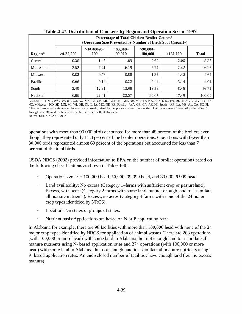
4-39

Table 4-47. Distribution of Chickens by Region and Operation Size in 1997.

Region a

Percentage of Total Chicken Broiler Counts b


>0-30,000>30,00060–

000>60,000–

90,000>90,000–180,000 >180,000 Total

Central 0.36 1.45 1.89 2.60 2.06 8.37

Mid-Atlantic 2.52 7.41 6.19 7.74 2.42 26.27

Midwest 0.52 0.78 0.58 1.33 1.42 4.64

Pacific 0.06 0.14 0.22 0.44 3.14 4.01

South 3.40 12.61 13.68 18.56 8.46 56.71

National 6.86 22.41 22.57 30.67 17.49 100.00a Central = ID, MT, WY, NV, UT, CO, AZ, NM, TX, OK; Mid-Atlantic = ME, NH, VT, NY, MA, RI, CT, NJ, PA, DE, MD, VA, WV, KY, TN,NC; Midwest = ND, SD, MN, MI, WI, OH, IN, IL, IA, MO, NE, KS; Pacific = WA, OR, CA, AK, HI; South = AR, LA, MS, AL, GA, SC, FL.

b Broilers are young chickens of the meat-type breeds, raised for the purpose of meat production. Estimates cover a 12-month period (Dec. 1through Nov. 30) and exclude states with fewer than 500,000 broilers.Source: USDA NASS, 1999c.

operations with more than 90,000 birds accounted for more than 48 percent of the broilers eventhough they represented only 11.3 percent of the broiler operations. Operations with fewer than30,000 birds represented almost 60 percent of the operations but accounted for less than 7percent of the total birds.

USDA NRCS (2002) provided information to EPA on the number of broiler operations based onthe following classifications as shown in Table 4-48:

• Operation size: > = 100,000 head, 50,000–99,999 head, and 30,000–9,999 head.

• Land availability: No excess (Category 1–farms with sufficient crop or pastureland).Excess, with acres (Category 2 farms with some land, but not enough land to assimilateall manure nutrients). Excess, no acres (Category 3 farms with none of the 24 majorcrop types identified by NRCS).

• Location:Ten states or groups of states.

• Nutrient basis:Applications are based on N or P application rates.

In Alabama for example, there are 98 facilities with more than 100,000 head with none of the 24major crop types identified by NRCS for application of animal wastes. There are 268 operations(with 100,000 or more head) with some land in Alabama, but not enough land to assimilate allmanure nutrients using N- based application rates and 274 operations (with 100,000 or morehead) with some land in Alabama, but not enough land to assimilate all manure nutrients using P- based application rates. An undisclosed number of facilities have enough land (i.e., no excessmanure).

4-40

Table 4-48. Number of Broiler Facilities as Provided by USDA Based on Analyses of 1997Census of Agriculture Database.

Location Land availability category Operation Size and Nutrient Basis> = 100,000 50,000–99,999 30,000–49,999N P N P N P

AL No excess d d 34 15 39 32AL Excess, no acres 98 98 227 227 217 217AL Excess, with acres 268 274 666 685 412 419AR No excess d d 58 49 104 93AR Excess, no acres 69 69 155 155 226 226AR Excess, with acres 260 263 797 806 672 683GA No excess d d 17 6 14 10GA Excess, no acres 169 169 319 319 194 194GA Excess, with acres 382 387 494 505 250 254KT, TN, VA, WV No excess d d 34 17 23 15KT, TN, VA, WV Excess, no acres 58 58 169 169 129 129KT, TN, VA, WV Excess, with acres 187 201 304 321 149 157MD, DE No excess d d 106 31 103 38MD, DE Excess, no acres 62 62 275 275 294 294MD, DE Excess, with acres 38 73 146 221 107 172MS No excess d d 10 8 14 14MS Excess, no acres 72 72 172 172 70 70MS Excess, with acres 230 230 437 439 143 143NC, SC No excess d d 61 12 59 19NC, SC Excess, no acres 105 105 287 287 290 290NC, SC Excess, with acres 177 198 394 443 292 332OK, MO, KS No excess d d 19 12 30 29OK, MO, KS Excess, no acres 26 26 49 49 32 32OK, MO, KS Excess, with acres 124 126 248 255 171 172TX, LA No excess d d 23 21 9 8TX, LA Excess, no acres 53 53 117 117 41 41TX, LA Excess, with acres 231 231 312 314 86 87other No excess d d 41 11 45 17other Excess, no acres 113 113 162 162 112 112other Excess, with acres 100 104 190 220 99 127Source: USDA NRCS, 2002.d = data not disclosed

4.2.1.2 Production Cycles of Broilers

Broilers are usually grown for 42 to 56 days depending on the market weight desired. Femalebroilers can also be grown to lay eggs for replacement stock, and these females are called broilerbreeders. Roasters are usually grown separated by sex, with the females being harvested at 42days of age and the males given the space in the entire house until they are sent to market severalweeks later (USEPA, 1998). Other meat-type chickens (capons, game hens) comprise less than 1percent of chickens raised for meat. Since they are raised in a similar manner to broilers, albeitwith different market weights and ages, they are not usually differentiated in the data.

Chickens are produced to meet specific requirements of the customer which can be a retail outlet,fast-food chain, or institutional buyer, among others. A broiler is considered any chicken raised

4-41

for meat products, though the industry further classifies chickens primarily by the size, weight,and age of the bird when processed.

• Poussin - Less than 24 days of age and about 1 pound or less.

• Cornish Game Hens - Less than 30 days of age and about 2 pounds.

• Fast-food Broiler - 2 pounds, 4 ounces to 3 pounds, 2 ounces (mostly 2 pounds, 6ounces to 2 pounds, 14 ounces) and less than 42 days of age.

• 3's and Up - 3 to 4 3/4 pounds and 40 to 45 days of age.

• Broiler Roaster - 5 to 6 pounds, hens usually 55 days.

• Broiler for Deboning - 5 to 6 pounds, males usually 47 to 56 days.

• Heavy Young Broiler Roaster - The typical roaster, 6 to 8 pounds, less than 10 weeks.

• Capon - 7 to 9 pounds, surgically desexed male broiler, 14 to 16 weeks.

• Heavy Hens - spent breeder hens, 5 to 5 ½ pounds, 15 months of age.

4.2.1.3 Broiler Facility Types and Management

The most common type of housing for broilers, roasters, pullets, and breeding stock is some typeof enclosed housing with bedding derived from wood shavings, rice hulls, chopped straw, peanuthulls, or other products, depending on availability. The bedding absorbs moisture and dilutes themanure produced by the birds. Modern houses have an automatic feeding system to distribute thefeed, a closed water system (automatic) to deliver the water for the birds, and a ventilationsystem to provide clean air. Some houses have side curtains that can be retracted to allowdiffusion of air. Ventilation is typically provided using a negative-pressure system, with exhaustfans drawing air out of the house, and fresh air returning through ducts around the perimeter ofthe roof. The ventilation system uses exhaust fans to remove moisture and noxious gases duringthe winter season and excess heat during the summer. Advanced systems use thermostats andtimers to control exhaust fans. These houses are also commonly integrated with an alarm signalto notify the operator of malfunctions and a back-up electric generator during power outages.

Broilers and Roasters. Houses for broilers and roasters are usually 40 feet wide and 400 to 500feet long and typically designed for 25,000 to 30,000 broilers per flock. Older houses may besomewhat smaller, holding 20,000 to 25,000 birds. The houses contain an impermeable surfacefor the floor, typically clay. Wood shavings are initially added to the houses to a depth ofapproximately 4 inches. Between flocks, a small amount of litter referred to as cake (compactedand concentrated manure/litter mix) is removed and the remaining litter may be “top dressed”with an inch or so of new bedding material.

Pullets. Pullets are young chickens, usually less than 20 weeks of age, often raised for thepurpose of egg production. Pullet houses are similar in construction to broiler houses. The housesare usually 40 to 45 feet in width and 300 to 500 feet in length. Most pullet houses are equippedwith nipple, trough, or bell drinkers and often use mechanical feeders (drag chain, trough, or pan)

4-42

to distribute feed to the birds. Pullets are usually raised on a floor covered with a bedding source,1 to 4 inches deep. This litter mixture is either removed after each flock (20 to 21 weeks) or usedfor a second flock. If the litter is used for a second flock, a small amount of litter as cake isremoved and the remaining litter is top dressed with an inch or so of new bedding material.When the house is totally cleaned out, the litter is pushed to the center of the house and a frontloader places it in a litter spreader for land application or disposal. Regular and thorough housecleaning is required to minimize disease transmission.

Breeders. Houses are usually 40 to 45 feet in width and 300 to 600 feet in length. Most of thebreeder houses contain two rows of slats for the birds to roost. The slats are panels of woodelevated 18 to 24 inches and laid across supports. The slats are spaced 1 inch apart to allow thefeces material to fall to the floor. Equipment can access the center section of the house to aid inthe clean-out between flocks. These slats cover two-thirds of the entire length of the house alongthe outside walls, with the center one-third of the building containing bedding litter.

The center third of the house is covered with 2 to 6 inches of a bedding source before youngbreeder layers are placed in the breeder house. Drinkers, mechanical feeders, and nests are placedover the slat section of the house, which allows most of the manure produced by the birds to fallbeneath the slat area, keeping the area accessible to the birds cleaner.

4.2.1.4 Broiler Waste Management Practices

This section summarizes waste management practices for broiler, breeding stock, pullets, androaster production facilities. Manure as excreted by the birds has a high water content, most ofwhich evaporates. A typical broiler house with capacity for 22,000 birds at a time will produce120 tons of litter per year. The litter consists mainly of wood chips or other organic plant mattereven after it has been in place for a year (NCC, 1999).

Litter Clean-out Schedules. The litter (bedding and manure) of broiler, pullet, and roasterhouses is typically cleaned out completely once a year, although there is a trend toward lessfrequent complete clean-outs. Between flocks, the feeders, waterers, and brooding equipment arewinched to the ceiling. A machine is often used to clean out any clumps of litter (termed cakingout) that may build up around waterers and feeders. When the broiler or roaster house iscompletely cleaned out, the litter is typically removed with a front-end loader or bobcat to aspreader truck or flail-type spreader. Spreader trucks are similar to lime-spreading trucks, with amoving bed that empties onto large, round metal plates that distribute the litter for use asfertilizer nutrients for pasture and crops. The rate of application is controlled by the rate at whichthe moving bed empties and the speed of the truck (NCSU, 1998a).

The common clean-out frequency in broiler breeder houses is once a year. When the house iscleaned, all the equipment (including slats) is removed from the house to allow a front-end loaderto push all of the manure to the center litter section of the house. Then a front-end loader placesthe mixture of manure and litter into a spreader for land application. A thorough cleaning aftereach flock (essentially once a year) removes pathogens that could be transferred to the next flock.After removal of all organic matter, the house is disinfected.

4-43

Litter Storage. Litter is removed from houses in large quantities during annual clean-out. Thus,operators that have land try to time the annual clean-out to coincide with the time land isavailable for litter application. If this approach is successful, the facility will need only enoughstorage for cake out during the rest of the year. Traditionally, operators stack litter outside, nearthe poultry houses or at the edge of fields for spreading in the spring.

However, an increasing number of states are imposing restrictions on the outdoor storage ofwaste, although the stringency of these requirements varies from state to state. For example,under Virginia’s Poultry Waste Management Program, stockpiled poultry litter must be (1)covered, (2) located to prevent storm water runoff, and (3) separated a minimum of 3 feet fromthe seasonally high water table or by the use of an impermeable barrier. Maryland’s requirementsfor outdoor storage are less restrictive and require only that storage be protected from rainfall andrunoff. The state of Delaware, which is also an important producer of poultry, is less restrictivethan Maryland and allows for uncovered storage of poultry litter (Hansen, 2000).

There are several methods for storing poultry litter ranging from open stock piles to roofedstorage structures. The size and type of method employed varies with location and size of theoperation as well as applicable regulations. Open stockpiles are the least expensive alternative,but pose the greatest risk of contaminating the surrounding environment. Contamination risk isreduced if these stockpiles are put on top of ground liners. Other storage structures includebunker-type storage structures, which are permanent aboveground concrete slabs with twoparallel walls of concrete identical to those used for storing silage on livestock farms (Brodie etal., 2000). Storage structures with permanent roofs offer both advantages and disadvantages.These structures eliminate the need for plastic covers and reduce the risk of runoffcontamination; however, they require a higher level of investment and higher maintenance coststhan the other types of structures. Also if these roof structures are not high enough, compactingbecomes more difficult and reduces the operator’s ability to use the full capacity of the structure(Goan, 2000).

4.2.1.5 Pollution Reduction

New technologies in drinking water systems result in less spillage and are equipped withautomatic shutoff valves that help ensure that broiler litter stays drier. Feeding strategies reducethe quantity of waste generated by ensuring that broilers do not receive more feed than requiredfor optimal growth. State regulations have also driven many broiler operations to handlemortalities in ways other than burials such as rendering and composting, which are increasing(see Section 4.2.1.6).

Nipple water delivery systems reduce the amount of wasted water and are healthier for theanimals. Trough or bell type watering devices allow the animal to spill water and addcontaminants to the standing water. Nipple water systems deliver water only when the animal issucking on the nipple. Watering systems may also use water pressure sensors with automaticshutoff valves to reduce water spillage. The sensor will detect a sustained drop in water pressureresulting from a break in the water line. The sensor will then stop the water flow to the broken

4-44

line and an alarm will sound. The operator can then fix the broken line and restore water to theanimals with minimal water spillage.

Feeding strategies that reduce N and P can reduce the quantity of nutrients in the excreta. Dietarystrategies designed to reduce N and P include enhancing the digestibility of feed ingredients,genetic enhancement of cereal grains and other ingredients resulting in increased feeddigestibility, more precise diet formulation, and improved quality control. Although N and P arecurrently the focus of attention, these strategies also have the potential to decrease othernutrients. Phytase is commonly added to broiler feed. Phytase additions are expected to achieve areduction in P excretion of 20 to 60 percent depending on the P form and concentration in thediet (NCSU, 1998b). Protein content, calcium, other mineral content, vitamin B, and otherfactors identified in the literature influence the effectiveness of phytase use in feed. Additionalinformation on feeding strategies for broilers can be found in Chapter 8.

Feeding Strategies. P excretion can be reduced by improving the utilization of feed nutrientsthrough genetic improvements in poultry or by improving the availability of nutrients in the feedingredients through processing or genetics. Absorption of some minerals is relatively poor and isdependent on the chemical form in the feed or supplement.

4.2.1.6 Waste Disposal

This section summarizes waste disposal practices for poultry production facilities. The two majorcategories of poultry waste are manure or litter (manure mixed with bedding) and dead animals.There is little variation in manure characteristics, but the litter composition varies by storage,composting management, and other practices. Poultry litter can be disposed of in several waysincluding land application, animal feed, and incineration. Waste may be pelletized before itsapplied to the land. Pelletizing produces a more uniform product that is lighter, easily transportedin bulk, and spread more uniformly. Additional information on pelletizing poultry wastes andother waste disposal methods can be found in Chapter 8.

Land Application of Poultry Litter. Land application of poultry litter recovers nutrients thatotherwise would be lost, and improves crop yields. Poultry manure slowly releases its nutrients,so annual applications are possible. Composting and bagging a pelleted poultry manure fertilizerproduces a marketable product for the commercial horticulture industry. One main obstacle togreater commercialization of poultry manure as a fertilizer product has been the inconsistency inproduct quality from one facility to another.

Where land application is employed, operators commonly use broadcast spreaders and flail-typespreaders for litter. Recommended application rates are based on the nutrient content of the litter,crop type and yield goals, and current soil conditions.

Many producers with cropland apply their litter to their own crops. However, as operations haveincreased in size and become more specialized, this option is becoming more limited. In somecases, poultry production provides supplemental income to an otherwise small or nonagriculturalhousehold with little or no land. Further exacerbating the problem of poultry litter disposal is the

4-45

fact that many areas of chicken production have a surplus of nutrient supply over crop needs(USDA NRCS, 1998). In these areas, poultry producers face difficulties in selling litter, givinglitter away, or even paying local farmers to take the litter. Table 4-48 presents the number ofbroiler operations with and without adequate crop and pastureland for manure application on anN- and P- basis at plant removal rates and operations that own no land. The operations that haveno land were determined by running queries of the USDA 1997 Census of Agriculture data toidentify facilities that did not grow any of the 24 major crops grown in the United States.Operations with no land available are assumed to haul their waste to land that can use the wasteas a fertilizer resource. More details on the national- and county-level nutrient balance are foundin Chapter 6.

Use of Poultry Litter as Animal Feed. Data on the use of poultry litter as animal feed isinadequate to determine how prevalent it is as a waste disposal method. Anecdotal informationindicates that use of poultry litter as a food supplement for beef herds may be common in theMid-Atlantic and Southeast Regions.

Incineration of Poultry Wastes. Incineration of poultry wastes is not done on a large scale inthe United States. The practice is being successfully implemented in the United Kingdom and isactively being investigated in this country. Additional information on centralized incineration ofpoultry wastes is presented in Chapter 8.

Disposal of Dead Animals. Concerns about possible ground water pollution from the burial ofdead birds have caused the poultry industry to search for alternatives for dealing safely with deadstock. The most common methods of disposal of dead birds are composting, incineration, burialin deep pits, rendering, and disposal in landfills. Anecdotal information indicates that somebroiler integrators have begun to distribute freezers to grower operations to store dead birds priorto picking them up for rendering. Technical information on practices for the disposal of deadanimals is presented in Chapter 8. However, there is little information available on the relativeuse of these practices within the broiler industry.

4.2.2 Layer Sector

This section describes the following aspect of the layer industry:

• 4.2.2.1: Distribution of the layer industry by size and region

• 4.2.2.2: Production cycles of layers and pullets

• 4.2.2.3: Layer facility types and management

• 4.2.2.4: Layer waste management practices

• 4.2.2.5: Egg processing and wash water



4-46

National Overview. Trends in the egg production subsector have paralleled those in otherlivestock industries—increasing overall production on fewer and larger farms. At the end of1997, there were 69,761 operations with hens and pullets of laying age (layers 20 weeks andolder) in the United States. This number represents a 19 percent decrease from the estimated86,245 operations with egg-producing birds in 1992 (USDA NASS, 1999c). In the 10-year periodfrom 1982 to 1992, the number of operations with hens and pullets declined from more than212,000, a 60 percent decrease (Abt, 1998). Table 4-49 shows the number of operations and birdinventory for 1982, 1987, 1992, and 1997. The number of operations in each category ofoperation has decreased substantially while total production has increased. Table 4-49 alsoprovides data on operations and inventory with birds below laying age. As with other sectors,specialization of production has gained a foothold, with a small but increasing number ofoperations producing only pullets.

Table 4-49. Operations With Inventory of Layers or Pullets 1982-1997.Total

Number of Farms with

1997 1992 1987 1982

Ops Production Ops Production Ops Production Ops Production

Layers 20weeks andolder

69,761 313,851,480 86,245 301,467,288 141,880 316,503,065 212,608 310,515,367

Layer andpullets 13weeks andolder

72,616 366,989,851 88,235 351,310,317 144,438 373,577,186 215,812 362,464,997

Pulletsbetween 13and 20 weeksold

13,180 53,138,371 14,818 49,843,029 19,639 57,074,121 28,109 51,949,630

Pullets lessthan 13 weeks

5,122 51,755,985 4,938 44,567,993 6,753 47,409,798 8,726 40,705,085


One major difference between the layer and egg production sector and the broiler productionsector is geographical distribution. Layer production, although primarily performed in 10 states,is much less geographically concentrated than the broiler industry. Hence, the key regionsidentified for the broiler industry in the previous section are not applicable to the layer and eggproduction sector. Overall, layer production has not increased as rapidly as has broilerproduction.

4.2.2.1 Distribution of Layer Operations by Size and Region

Layers are defined as chickens maintained for the production of table eggs. Eggs may beproduced for human consumption in the shell form (sold in cartons) or may be used in theproduction of liquid, frozen, or dehydrated eggs. Laying hen operations include facilities that

4-47

confine chickens for feeding or maintenance for at least 45 days in any 12-month period. Thesefacilities do not have significant vegetation in the confinement area during the normal growingseason. Facilities that raise pullets are generally included. Egg washing and egg processingfacilities located at the same site as the birds are generally included. Facilities that have layinghen or pullet feeding operations may also include animal and agricultural operations such asgrazing and crop farming.

EPA’s 1974 CAFO ELG generally apply to laying hen operations with more than 100,000 birdsand with continuous overflow watering systems, and to laying hen operations with 30,000 birdsand with a liquid manure system. (See Chapter 2 for the definition of a CAFO, and Chapter 5 fora discussion of the basis for revisions to the poultry subcategories.) Where numbers of birds arepresented, all birds regardless of age (e.g., poult, laying age, or pullet) or function (i.e., breeder,layer, meat-type chicken) are included unless otherwise indicated in the text.

Table 4-50 presents the number of layer, pullet, and combined operations by size class as well asthe average bird count at each type of operation. Table 4-51 presents the number of operationswith laying hens by operation size and region. Data on the three types of operations wereobtained through special queries of the 1997 Census of Agriculture (USDA NASS, 1999c). Eachoperation is uniquely characterized, thus the sum of all three provides the total number ofoperations with layers or pullets or both (75,172 total operations). Pullet operations wereassumed to be evenly distributed so as to support layer operations. Table 4-52 presents thedistribution of egg laying chickens by facility size and region. It is important to note that in 1997the 326 largest operations with laying hens were less than one half of a percent of the totaloperations (70,857) but had over 55 percent of the laying hens. Table 4-53 presents the numberof layer facilities and total USDA-based AUs using the 1997 Census of Agriculture (USDANRCS, 2002).

Table 4-50. Number of Operations in 1997 and Average Number of Birds at Operations with Layers or Pullets or Both Layers and Pullets in 1997.

NationalItem

Number of Layer, Pullet, and combined Layer and Pullet Operations and Average BirdCounts (Operation Size Presented by Number of Birds Spot Capacity)

>0–30,000>30,000–

62,500>62,500–180,000

>180,000–600,000 >600,000 Total

Layer Ops 57,413 528 419 146 25 58,531

Layer Count 926 43,621 103,048 311,189 1,013,318

Pullet Ops a 3,694 516 61 44 4,315

Pullet Count 5,010 51,162 133,303 305,679

Layer andPullet Ops

12,011 67 93 91 64 12,326

Layer andPullet Count

218 45,963 112,377 358,580 1,367,476

a Pullet size ranges vary from the others: >0-30,000; >30,000-100,000; >100,000-180,000; and >180,000.Source: USDA NASS, 1999c.

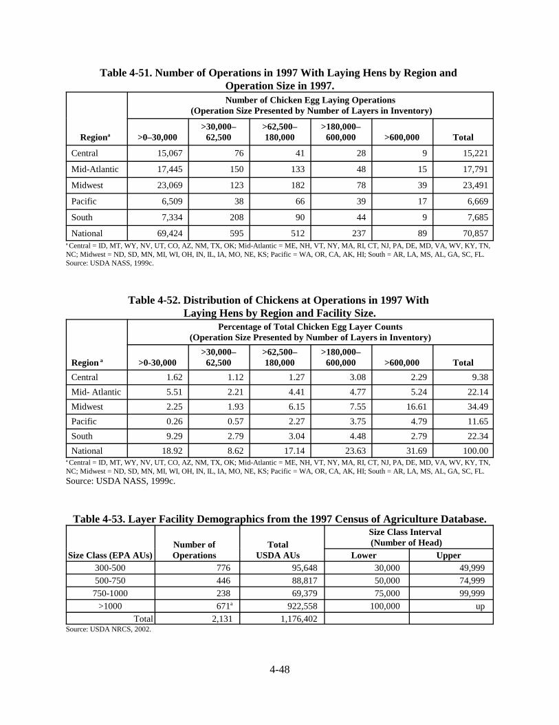
4-48

Table 4-51. Number of Operations in 1997 With Laying Hens by Region and Operation Size in 1997.

Regiona

Number of Chicken Egg Laying Operations (Operation Size Presented by Number of Layers in Inventory)

>0–30,000>30,000–

62,500>62,500–180,000

>180,000–600,000 >600,000 Total

Central 15,067 76 41 28 9 15,221

Mid-Atlantic 17,445 150 133 48 15 17,791

Midwest 23,069 123 182 78 39 23,491

Pacific 6,509 38 66 39 17 6,669

South 7,334 208 90 44 9 7,685

National 69,424 595 512 237 89 70,857a Central = ID, MT, WY, NV, UT, CO, AZ, NM, TX, OK; Mid-Atlantic = ME, NH, VT, NY, MA, RI, CT, NJ, PA, DE, MD, VA, WV, KY, TN,NC; Midwest = ND, SD, MN, MI, WI, OH, IN, IL, IA, MO, NE, KS; Pacific = WA, OR, CA, AK, HI; South = AR, LA, MS, AL, GA, SC, FL.Source: USDA NASS, 1999c.

Table 4-52. Distribution of Chickens at Operations in 1997 With Laying Hens by Region and Facility Size.

Region a

Percentage of Total Chicken Egg Layer Counts(Operation Size Presented by Number of Layers in Inventory)

>0-30,000>30,000–

62,500>62,500–180,000

>180,000–600,000 >600,000 Total

Central 1.62 1.12 1.27 3.08 2.29 9.38

Mid- Atlantic 5.51 2.21 4.41 4.77 5.24 22.14

Midwest 2.25 1.93 6.15 7.55 16.61 34.49

Pacific 0.26 0.57 2.27 3.75 4.79 11.65

South 9.29 2.79 3.04 4.48 2.79 22.34

National 18.92 8.62 17.14 23.63 31.69 100.00a Central = ID, MT, WY, NV, UT, CO, AZ, NM, TX, OK; Mid-Atlantic = ME, NH, VT, NY, MA, RI, CT, NJ, PA, DE, MD, VA, WV, KY, TN,NC; Midwest = ND, SD, MN, MI, WI, OH, IN, IL, IA, MO, NE, KS; Pacific = WA, OR, CA, AK, HI; South = AR, LA, MS, AL, GA, SC, FL.

Source: USDA NASS, 1999c.

Table 4-53. Layer Facility Demographics from the 1997 Census of Agriculture Database.

Size Class (EPA AUs)Number ofOperations

Total USDA AUs

Size Class Interval (Number of Head)

Lower Upper300-500 776 95,648 30,000 49,999

500-750 446 88,817 50,000 74,999

750-1000 238 69,379 75,000 99,999

>1000 671a 922,558 100,000 up

Total 2,131 1,176,402Source: USDA NRCS, 2002.

4-49

4.2.2.2 Production Cycles of Layers and Pullets

A layer is a sexually mature female chicken capable of producing eggs. Egg production can bedivided into two types, table and hatching. Table eggs are used for consumption, and hatchingeggs are used to supply broiler or layer production operations.

Traditionally, layers are kept through 1 year of egg production and sold for meat at 18 to 20months of age. Depending on market conditions (relative price of eggs to hens), it has becomeincreasingly common to recycle layers through more than 1 year of production (Bradley et al.,1998). Producers will recycle their flocks into a second or even a third cycle of lay. Flockrecycling involves stopping the flock’s egg production, allowing a suitable rest period, and thenbringing the flock back into production. The entire process (called “force molting”) of recyclinglayers takes approximately 4 to 5 weeks. Producers stop egg production by reducing the length ofday (lighting) and feed supply. This period typically takes 2 to 4 weeks and involves a 7-day fast followed by a period during which the flock is fed a low calcium diet. After this “rest period,” theflock is returned to normal lighting conditions and a nutritionally balanced diet to support eggproduction (UCD, 1998). Once the flock is brought back into production, most layers will meetor exceed original levels of egg production. Under this regime, the flock’s life is extended for 6to 12 additional months.

4.2.2.3 Layer Facility Types and Management

Litter-based Housing. A few litter and slat/litter houses are used to produce table eggs. Thesesame housing systems are used for the breeders that produce fertile eggs for the production ofhatching eggs, which eventually replace the current flock of egg layers.

Non-litter Based Housing. Layers are often raised in cages arranged in two or four decks. Cageshave been the preferred way of housing table egg layers since the mid-1940s (Bradley et al.,1998). They are popular because they provide good sanitation. When the birds are caged, flocknutrition can be better managed and products (eggs) kept cleaner. Cages are designed to separatethe layers from their own feces and thereby eliminate many of the feces-related parasite andhealth problems. Most commercial layer facilities employ one of the following designs.

High-rise Cage Systems. Cage systems are two-story poultry houses with cages for the layinghens in the top story suspended over the bottom story, where the manure is deposited and stored.The house structure itself is usually 40 to 60 feet wide and from 400 to 500 feet long. Thewatering system is a closed (noncontinuous flow) nipple or cup system. The ventilation system isdesigned so that the external air is brought into the top story, through the cages where the birdsare located, and then over the manure in the bottom story, exiting through fans in the bottomstory side wall. The ventilation system is designed to dry manure as it is stored. With propermanagement of waterers to prevent water leaking to the bottom story, layer waste commonly hasa moisture content of 30 to 50 percent.

Scrape-out and Belt Systems. Housing facilities for scrape-out and belt manure removal cagesystems are the same dimensions as high-rise units except they have only one story. Watering

4-50

systems in these operations are also closed, using nipple or cup waterers. Ventilation varies fromfan-controlled to adjustable curtains in the side wall.

Cages in the scrape-out system are suspended over a shallow pit, which is scraped out to the endof the house by a small tractor or a pit scraper. Belt systems have a continuous belt under thedifferent tiers of cages that moves the manure to the end of the house, where it is placed into afield spreader or some other suitable storage device. Some of the newer belt systems move airover the manure on the belt in an attempt to dry the manure before it is removed.

The manure from scrape-out and belt systems usually has a moisture content of between 70 and85 percent. Therefore, the manure can be handled as a slurry, which is either injected or landapplied to the land with a spreader that can handle the high-moisture manure.

Flush-Cage Housing. Housing, equipment, and ventilation in flush-cage housing are similar tothe scrape-out system with the exception of how the manure is handled. Cages are suspendedover a shallow pit as in the scrape-out system, but water is used to move the manure from underthe cages to the end of the house, where the water and manure mixture is placed in an anaerobiclagoon. The water used to flush the manure pits is recycled from the lagoon. A variation of thissystem consists of solids separation by means of a primary lagoon and a secondary lagoon(NCSU, 1998a).

Although storage, management, and disposal practices are quite similar for broiler and layeroperations, with the exception of layer operations using lagoon systems, there are regionaldifferences in how operations manage waste. A survey conducted by the United Egg Producersduring 1998 indicated significant regional differences in the way layer wastes are managed.These differences are shown in Table 4-54. This data was used with the data in Table 4-51 toestimate that the total number of layer operations that use water to move the wastes to a lagoon(referred to as wet layer systems) was approximately 3,100 operations.

Table 4-54. Summary of Manure Storage, Management, and Disposal.

Practice

Percentage of Region With Practice

Pacific Central MidwestMid-

Atlantic South

Storage sheds in addition to high-rise housing 0 0 10 0 0

Housing with 6-month or longer storage of dry manure 75 40 90 90 40

Export or sale of some or all of litter 100 40 100 75 50

Litter use other than land application (incineration,pelletization)

0 0 5 5 0

Farms with wet storage systems, such as lagoon 0 60 2 5 60

Source: UEP, 1998

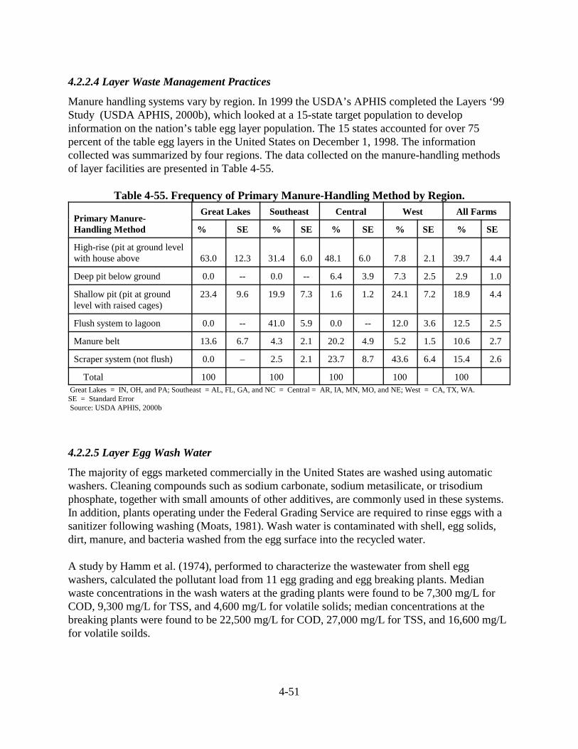
4-51

4.2.2.4 Layer Waste Management Practices

Manure handling systems vary by region. In 1999 the USDA’s APHIS completed the Layers ‘99Study (USDA APHIS, 2000b), which looked at a 15-state target population to developinformation on the nation’s table egg layer population. The 15 states accounted for over 75percent of the table egg layers in the United States on December 1, 1998. The informationcollected was summarized by four regions. The data collected on the manure-handling methodsof layer facilities are presented in Table 4-55.

Table 4-55. Frequency of Primary Manure-Handling Method by Region.

Primary Manure-Handling Method

Great Lakes Southeast Central West All Farms

% SE % SE % SE % SE % SE

High-rise (pit at ground levelwith house above 63.0 12.3 31.4 6.0 48.1 6.0 7.8 2.1 39.7 4.4

Deep pit below ground 0.0 -- 0.0 -- 6.4 3.9 7.3 2.5 2.9 1.0

Shallow pit (pit at groundlevel with raised cages)

23.4 9.6 19.9 7.3 1.6 1.2 24.1 7.2 18.9 4.4

Flush system to lagoon 0.0 -- 41.0 5.9 0.0 -- 12.0 3.6 12.5 2.5

Manure belt 13.6 6.7 4.3 2.1 20.2 4.9 5.2 1.5 10.6 2.7

Scraper system (not flush) 0.0 – 2.5 2.1 23.7 8.7 43.6 6.4 15.4 2.6

Total 100 100 100 100 100 Great Lakes = IN, OH, and PA; Southeast = AL, FL, GA, and NC = Central = AR, IA, MN, MO, and NE; West = CA, TX, WA.SE = Standard Error Source: USDA APHIS, 2000b

4.2.2.5 Layer Egg Wash Water

The majority of eggs marketed commercially in the United States are washed using automaticwashers. Cleaning compounds such as sodium carbonate, sodium metasilicate, or trisodiumphosphate, together with small amounts of other additives, are commonly used in these systems.In addition, plants operating under the Federal Grading Service are required to rinse eggs with asanitizer following washing (Moats, 1981). Wash water is contaminated with shell, egg solids,dirt, manure, and bacteria washed from the egg surface into the recycled water.

A study by Hamm et al. (1974), performed to characterize the wastewater from shell eggwashers, calculated the pollutant load from 11 egg grading and egg breaking plants. Medianwaste concentrations in the wash waters at the grading plants were found to be 7,300 mg/L forCOD, 9,300 mg/L for TSS, and 4,600 mg/L for volatile solids; median concentrations at thebreaking plants were found to be 22,500 mg/L for COD, 27,000 mg/L for TSS, and 16,600 mg/Lfor volatile soilds.

4-52

Eggs may be washed either on or off farm. Operations that wash their eggs on farm may do soinline or offline. The frequency of egg processing by location is presented in Table 4-56. Thefrequency of egg processing by operation size is presented in Table 4-57. Eggs from over 80percent of the operations are processed off site. Operations with fewer than 100,000 layers aremore likely to have their eggs processed off site. Smaller poultry operations primarily haul theirwash water to treatment centers or sell their eggs to larger operations for washing and processing(Thorne, 1999). On the other hand, larger egg production operations collect and store egg washwater on site in large tanks or lagoons for treatment and storage. This lagoon water may then beapplied to fields using spray irrigation. These anaerobic lagoons are earthen structures designedto provide biological treatment and long-term storage of poultry layer waste. Treatment of wasteoccurs anaerobically, a process in which organic material is decomposed to carbon dioxide andwater, while stabilized products, primarily humic substances, are synthesized. Where space isavailable, two-stage lagoons may be constructed for better wastewater treatment and greatermanagement flexibility. The first stage contains only the treatment (permanent) volume andsludge volume while the second stage lagoon stores treated wastewater for irrigation andprovides additional treatment that produces a higher quality effluent for recycling as flush water(Tyson, 1996).

Table 4-56. Percentage of Operations by Egg Processing Location and Region.

Primary EggProcessing Location

Great Lakes Southeast Central West All

% SE % SE % SE % SE % SE

On farm in line 17.8 8.4 13.1 4.3 9.0 3.2 10.9 2.4 13.5 3.0

On farm off line 6.7 5.4 0.6 0.6 3.3 3.3 9.3 2.4 5.3 2.1

Off farm 75.5 8.1 86.3 4.4 87.7 4.5 79.8 3.6 81.2 3.2

Total 100 -- 100 -- 100 -- 100 -- 100 --Regions: Great Lakes = IN, OH, and PA; Southeast = AL, FL, GA, and NC; Central = AR, IA, MN, MO, and NE; West = CA, TX, WA.SE = Standard Error.Source: USDA APHIS, 2000b.

Table 4-57. Percentage of Operations by Egg Processing Location and Operation Size.

Primary EggProcessing Location

Egg Laying Operations with<100,000 Layers

Egg Laying Operations with 100,000+Layers

% SE % SE

On farm in line 4.3 2.8 28.9 5.6

On farm off line 5.2 3.1 5.5 1.9

Off farm 90.5 4.1 65.6 6.0

Total 100 -- 100 --Regions: Great Lakes: IN, OH, and PA; Southeast: AL, FL, GA, and NC; Central: AR, IO, MN, MO, and NE; West: CA, TX, WA.SE = Standard Error.Source: USDA NAHMS, 2000.

4-53

4.2.2.6 Waste and Wastewater Reductions

Methods to reduce the quantity of wastewater generated at layer operations include advancedwatering systems to reduce water spillage and feeding strategies. The use of feeding strategieswill reduce the quantity of waste generated by ensuring that animals do not receive more feedthan required for optimal growth. Dietary strategies to reduce N and P content includedeveloping more precise diets and improving the digestibility of feed ingredients through the useof enzyme additives and genetic enhancement of cereal grains. Information on feeding strategiesfor layer operations can be found in Chapter 8.

There are several types of water delivery systems used in layer operations. Nipple water deliverysystems reduce the amount of wastewater and result in healthier birds. Trough or cup drinkersallow the bird to spill water and add contaminates to the standing water. Continual overflowwatering systems reduce the health risk to the birds but produce a greater quantity of wastewater.

Nipple water delivery systems are placed in the cage and deliver water only when the bird issucking on the nipple. Approximately 62 percent of all layer operations use nipple drinkersystems (USDA APHIS, 2000b). However, for layer operations with more than 100,000 birdsthis number increases to approximately 81.5 percent (USDA NAHMS, 2000). Watering systemsmay also use water pressure sensors and automatic shutoff valves to reduce water spillage. Thesensor will detect a sustained drop in water pressure resulting from a break in the water line. Thesensor will then stop the water flow to the broken line and an alarm will sound. The operator canthen fix the broken line and restore water to the animals with minimal water spillage. There islittle information about the relative use of water pressure sensors within the layer industry.


Practices for the disposal of layer wastes are similar to those for other poultry litter. Afterremoval from the housing facilities, waste can be directly applied to the land (if available), storedprior to final disposal, or pelletized and bagged for use as commercial fertilizer. Waste storage,application of litter, and other poultry waste disposal practices are discussed in detail in Section4.2.1.6. The percentage of layer and pullet operations with and without enough land forapplication of manure on a N- and P- basis and operations with no land are shown in Tables 4-58and 4-59. The facilities that have no land were determined by running queries of the USDA 1997Census of Agriculture data to identify facilities that did not grow any of the 24 major cropsgrown in the United States.

Mortality and the disposal of dead hens is a potentially significant source of contamination atlaying operations. A total of 6.5 percent of hens placed in the last completed flock (one flock perfarm site) died by 60 weeks of age, and the overall average cumulative mortality was 14.6percent (USDA APHIS, 2000b). The common methods of disposing of dead hens and frequencyof use are presented in Table 4-60. Tables 4-61 and 4-62 present this information for operationswith fewer than and more than 100,000 laying hens. Larger facilities are much more likely thansmaller facilities to send dead birds to rendering plants (50.2 percent versus 21.1 percent). While

4-54

smaller facilities are more likely than larger facilities to bury their dead birds (45.6 percent versus9.1 percent).

Table 4-58. Percentage of Layer Dominated Operations With Sufficient, Insufficient, andNo Land for Agronomic Application of Generated Manure.

Capacity(Number of

Birds)

Sufficient Land Insufficient Land No Land

Nitrogen Phosphorus Nitrogen Phosphorus

1–29,999 12.2 9.2 49.1 53 41.1

30,000–59,999 6.8 1 60.3 65 33.2

60,000–179,999 6.2 0 52 62.2 36.8

180,000+ 1.1 0 46.6 47.1 52.9

Total 10.5 6.9 49.5 57.5 38.8Source: USDA NASS, 1999c.

Table 4-59. Percentage of Pullet Dominated Operations With Sufficient, Insufficient, andNo Land for Agronomic Application of Generated Manure.

Capacity(Number of

Birds)

Sufficient Land Insufficient Land No Land

Nitrogen Phosphorus Nitrogen Phosphorus

1–29,999 11.6 5.9 47.3 53 41.1

30,000–59,999 11.9 1.7 54.9 65 33.2

60,000–179,999 14.1 1.1 49.2 62.2 36.8

180,000+ 2 0 45.1 47.1 52.9


Table 4-60. Frequency of Disposal Methods for Dead Layers for All Facilities.

Method of DisposalFarm Sites Dead Hens

Percent Std Error Percent Std Error

Composting 15.0 (3.5) 11.7 (4.1)

Incineration 9.0 (2.9) 10.4 (4.5)

Covered deep pit 32.0 (5.8) 17.9 (4.3)

Rendering 32.0 (4.9) 41.4 (8.6)

Other 16.1 (3.6) 18.6 (5.4)

Total -- 100.0Source: USDA APHIS, 2000b.

4-55

Table 4-61. Frequency of Disposal Methods for Dead Layers for Facilities With <100,000 Birds.



Composting 13.9 4.7 13.4 7.5

Incineration 9.3 4.2 19.8 9.8

Covered deep pit 45.6 7.2 36.4 8.3

Rendering 21.1 4.5 19.7 6.0

Other 14.0 4.7 10.7 3.8

Total -- -- 100.0 --Source: USDA NAHMS, 2000.

Table 4-62. Frequency of Disposal Methods for Dead Layers for Facilities With > 100,000 Birds.



Composting 16.8 4.6 10.6 4.4

Incineration 8.7 3.3 4.6 2.5

Covered deep pit 9.1 2.2 6.5 2.5

Rendering 50.2 7.2 54.8 10.9

Other 19.7 5.8 23.5 8.7

Total -- -- 100.0 --Source: USDA NAHMS, 2000.

4.2.3 Turkey Sector

This section describes the following aspects of the turkey industry:

• 4.2.3.1: Distribution of the turkey industry by size and region

• 4.2.3.2: Production cycles of turkeys

• 4.2.3.3: Turkey facility types and management

• 4.2.3.4: Turkey waste management practices



National Overview

Turkey production has increased steadily over the past 2 decades and, as in the other poultrysectors, there has been a shift in production to fewer but larger operations. Between 1982 and1997, almost 21 percent of the turkey operations went out of business (USDA NASS, 1998b). As

4-56

shown in Table 4-63, the number of turkey operations decreased from 12,708 operations in 1992to 12,207 operations in 1997, a 4 percent decrease. The number of turkeys produced roseapproximately 10 percent between 1992 and 1997. The number of hens held for breeding,however, decreased by almost 6 percent during the same period.

As in the broiler industry, most turkeys are produced under contract production arrangements.For each contract arrangement, an integrator company provides the birds, feed, medicines, birdtransport, and technical help. The contract producer provides the production facilities and laborto grow the birds from hatchlings to market-age birds. In return, the contract producer receives aguaranteed price, which may be adjusted up or down based on the performance of the birdscompared with that of other flocks produced or processed by the company during the same spanof time. Some turkeys are raised by independent turkey producers. Even under this type ofproduction, however, the independent producer may arrange for feed, poults, medical care, andpossibly processing, through contracts. Finally, some turkeys are produced on farms owned bythe integrator company. The integrator company may also be the company that processes thebirds; however, some turkey integrators provide all services except the processing, which theintegrator arranges with a processing company.

Table 4-63. Turkey Operations in 1997, 1992, 1987, and 1982 With Inventories of Turkeys for Slaughter and Hens for Breeding.

Total FarmsWith

1997 1992 1987 1982

Ops Production Ops Production Ops Production Ops Production

Turkeys 6,031 307,586,680 6,257 279,230,136 7,347 243,336,202 7,498 172,034,935

Turkeys sold forslaughter

5,429 299,488,350 5,658 272,831,801 6,813 238,176,199 6,838 167,540,306

Turkey hens keptfor breeding

747 8,098,330 793 6,398,335 761 5,160,003 1,040 4,494,629


4.2.3.1 Distribution of Turkey Operations by Size and Region

EPA’s 1974 CAFO Effluent Limitations Guidelines and Standards generally apply to turkeyoperations with more than 55,000 birds. (See Chapter 2 for the definition of a CAFO, andChapter 5 for a discussion of the basis for revisions to the poultry subcategories.) Wherenumbers of birds are presented, all birds regardless of age (e.g., poult, laying age, or pullet) orfunction (i.e., breeder, layer, meat-type birds) are included unless otherwise indicated in the text.

The consolidation of the turkey industry has mirrored that of other livestock industries. Thenumber of turkey farms with fewer than 30,000 birds decreased from 5,113 in 1987 to only 3,378in 1997 (USDA NASS, 1999b). Concurrently, the number of operations with more than 60,000birds increased 26 percent from 1232 in 1987 to 1671 in 1997. Although these changes are not asdramatic as those for the swine or broiler industry, they are indicative of an industry that isundergoing a steady transformation into one dominated by large integrated operations.

4-57

Table 4-64 presents the number of turkey operations in 1997 by size and region. Table 4-65presents the distribution of turkey production by size of operation and region. It is important tonote that the 369 largest operations (2.7 percent) had 43.6 percent of the total turkey count. Thesetables reflect the use of 2.5 turns (flocks) per year. USDA NASS performed an analysis for EPAto estimate how variations in the estimated of number of turns per year would change the numberof potential CAFOs (operations with more than 55,000 birds). This analysis showed that therewould be only minor changes to the estimated number of CAFOs if the estimated number ofturns was adjusted to two or three turns.

State-level data from the 1997 Census of Agriculture (USDA NASS, 1999b) indicate that statesin the Midwest and Mid-Atlantic Regions account for more than 70 percent of all turkeysproduced. Key production states (determined by number of turkeys produced) are North Carolina,Minnesota, Virginia, Arkansas, California, and Missouri. Other states with significant productioninclude Indiana, South Carolina, Texas, Pennsylvania, and Iowa. Table 4-66 presents the numberof turkey facilities and total USDA-based AUs using the 1997 Census of Agriculture (USDANRCS, 2002).

Table 4-64. Number of Turkey Operations in 1997 by Region and Operation Size.

Region a

Number of Turkey Operations by Size(Operation Size Presented by Number of Birds Spot Capacity)

>0–16,500 >16,500–38,500 >38,500–55,000 >55,000 Total

Central 2,301 54 19 34 2,408

Mid-Atlantic 3,265 597 143 83 4,088

Midwest 4,016 493 121 142 4,772

Other 2,035 222 83 110 2,450

National 11,617 1,366 366 369 13,718a Central = ID, MT, WY, NV, UT, CO, AZ, NM, TX, OK; Mid-Atlantic = ME, NH, VT, NY, MA, RI, CT, NJ, PA, DE, MD, VA, WV, KY, TN,NC; Midwest = ND, SD, MN, MI, WI, OH, IN, IL, IA, MO, NE, KS; Other = WA, OR, CA, AK, HI, AR, LA, MS, AL, GA, SC, FL.Source: USDA NASS, 1999c.

Table 4-65. Distribution of Turkeys in 1997 by Region and Operation Size.

Region a

Percentage of Total Turkey Counts by Operation Size(Operation Size Presented by Number of Birds Spot Capacity)

>0–16,500 >16,500–38,500 >38,500–55,000 >55,000 Total

Central 0.64 1.22 0.80 5.20 7.85

Mid-Atlantic 4.93 13.18 5.73 7.15 30.99

Midwest 4.38 10.62 4.88 19.94 39.82

Other 1.48 5.18 3.35 11.34 21.34

National 11.43 30.20 14.75 43.62 100.00a Central = ID, MT, WY, NV, UT, CO, AZ, NM, TX, OK; Mid-Atlantic = ME, NH, VT, NY, MA, RI, CT, NJ, PA, DE, MD, VA, WV, KY, TN,NC; Midwest = ND, SD, MN, MI, WI, OH, IN, IL, IA, MO, NE, KS; Other = WA, OR, CA, AK, HI, AR, LA, MS, AL, GA, SC, FL.Source: USDA NASS 1999c.

4-58

Table 4-66. Turkey Facility Demographics from the 1997 Census of Agriculture Database.Size Class (EPA AUs) Number of

OperationsTotal

USDA AUs Size Class Interval (Number of Head)

Lower Upper300–500 875 360,475 16,500 27,499 500–750 478 306,632 27,500 41,249

750–1000 262 230,628 41,250 54,999 1000+ 388 915,367 55,000 up Total 2,003 1,813,102

Source: USDA NRCS, 2002.

4.2.3.2 Production Cycles of Turkeys

The growth of a turkey is commonly divided into two phases: brooding and grow-out. Thebrooding phase is the period of the poult’s life extending from 1 day to about 6 to 8 weeks.During this time, the poults are unable to maintain a constant body temperature and needsupplemental heat. Brooder stoves are used to keep the ambient temperature at 90 to 95 °F whenthe poults arrive; thereafter, the producer decreases the temperature by 5 °F for the next 3 weeksuntil the temperature reaches 75 °F. Poults are extremely susceptible to disease and are typicallyadministered special starter feeds containing antibiotics and a high percentage of protein. Onedifference between turkeys and broilers is that feeding strategies, such as the use of phytase toreduce P content in waste, are not employed with turkeys through the entire life cycle becausephytase is thought by some to inhibit bone development in poults. As with the broiler industry,further research in diet, nutrition, and the complex relationships between calcium, vitamins, andP may overcome this limitation.

The grow-out phase is the period in a turkey’s life between the brooding phase and the market orbreeding phase. Depending on the sex of the birds, the grow-out phase typically lasts up to 14weeks. Modern turkeys grow rapidly. A tom (male) poult weighs about ¼ pound at birth; at 22weeks it weighs almost 37 pounds. Hens (females) are usually grown for 14 to 16 weeks andtoms from 17 to 21 weeks before being marketed. Most operators start fewer toms than hens in agiven house to allow more space for the larger birds.

4.2.3.3 Turkey Facility Types and Management

Market and breeder turkeys are raised in similar housing systems. Typically, young turkey poultsare delivered to the operation on the day of, or the day after, hatching. The poults are placed inbarns called brooder houses. The brooder houses for turkeys are usually as wide as broiler andpullet houses but are usually only 300 to 400 feet long. The houses have an impermeable floorsurface made of either clay or cement. The floors are then covered with 3 to 4 inches of bedding.

As with broilers, ventilation is usually provided by a negative-pressure system, with exhaust fansdrawing air out of the house and fresh air returning through ventilation ducts around theperimeter of the roof. Some turkey houses have side curtains that can be retracted to allowdiffusion of air. More advanced ventilation systems use exhaust fans controlled by a thermostat

4-59

and timer. Brooding heaters are normally present in one-third to one-half of the house, for theearly stages of development. As the poults get older, they are usually released into the other two-thirds or half of the house and remain there until they are of market age. In some operations thepoults are moved to a specially designed grower house, where they stay until they are of marketage. Some operations will move poults to range.

The construction of the housing facilities varies by region and depends on climatic conditionsand production practices. Generally, in the southern and southeastern U.S. the houses are moreopen. The side walls of the houses are 6 to 8 feet high, with a 4- to 5-foot-wide opening coveredby wires and curtains. Since moderate winters are normal in the South and Southeast, the curtainscan contain the heat necessary to maintain a reasonable temperature within the commercialpoultry houses. In the northern and central states, most houses have solid side walls and containconsiderable insulation to combat the colder temperatures. These houses rely on exhaust fans ormoveable solid side walls during the hot summer days to diminish the effects of heat stress onthe birds.

These traditional systems are called two-age farms because two ages of birds can be on the farmat one time. Once the poults have been moved to the grower barn, the brooder house is totallycleaned out for another group of poults. This cleanup includes removal of all litter used duringthe brooding phase. The second group of poults occupies the brooder house while the first groupof birds is still in the grower barn. Operations in the Shenandoah Valley area of Virginia andWest Virginia are known to use a modification of the typical two-age management system. Underthis system the houses are longer. Poults may occupy one end of the house, while an older groupis being grown out at the other end. The birds do not have to be moved as often under thissystem.

The two-age farm system has served the turkey industry for more than 20 years. Currently,however, there are efforts to modify this system because of morbidity and mortality. Themodifications are directed at raising older birds in facilities removed from the poults. Thisapproach provides an opportunity to break any disease cycle that might put the birds, especiallythe younger ones, at increased risk (USEPA, 1998).

4.2.3.4 Turkey Waste Management Practices

For brooder facilities, the litter is removed after every flock of brooded poults. This practice isnecessary to provide the next group of poults with clean bedding to achieve the lowest possiblerisk of disease exposure. Poult litter may be composted between flocks to control pathogens andthen reused in the grow-out houses. For grower systems, the litter is removed once a year. Inbetween flocks, cake is removed and the old litter may be top-dressed with a thin layer of newbedding. For single-age farms, the bedding in the brooding section is moved to the growersection. New bedding is put in the brooder section, and the facilities are prepared for the nextgroup of poults.

4-60

4.2.3.5 Pollution Reduction

New technologies in drinking water systems result in less spillage and ensure that turkey litterstays drier. Feeding strategies will also reduce the quantity of waste generated by ensuring thatturkeys do not receive more feed than required for optimal growth. State regulations have alsodriven many turkey operations to handle mortalities in ways other than burial such as renderingand composting, which are on the rise (see Section 4.2.3.6).

Nipple water delivery systems reduce the amount of wasted water and are healthier for theanimals. Trough or bell type watering devices allow the animal to spill water and addcontaminants to the standing water. Nipple water systems deliver water only when the animal issucking on the nipple. Watering systems may also use water pressure sensors and automaticshutoff valves to reduce water spillage. The sensor will detect a sustained drop in water pressureresulting from a break in the water line. The sensor will then stop the water flow to the brokenline and an alarm will sound. The operator can then fix the broken line and restore water to theanimals with minimal water spillage.

Feeding strategies can be used to reduce the quantity of nutrients in the excreta. Dietary strategiesdesigned to reduce N and P include enhancing the digestibility of feed ingredients, geneticenhancement of cereal grains and other ingredients resulting in increased feed digestibility, moreprecise diet formulation, and improved quality control. Although N and P are currently the focusof attention, these strategies also have the potential to decrease other nutrients. There is debate onthe impacts of phytase feed supplements for turkey poults concerning bone growth and bonedevelopment. Phytase additions are expected to achieve a reduction in P excretion of 20 to 60percent depending on the P form and concentration in the diet (NCSU, 1998b). Protein content,calcium, other mineral content, vitamin B, as well as other factors identified in the literatureinfluence the effectiveness of phytase use in feed. Additional information on feeding strategiesfor turkeys can be found in Chapter 8.


Practices for the disposal of turkey litter are similar to those for other poultry litter. After removalfrom the housing facilities, waste can be directly applied to the land (if available), stored prior tofinal disposal, or pelletized and bagged for use as commercial fertilizer. Waste storage,application of litter, and other poultry waste management practices are discussed in detail inSection 4.2.1.4. The percentage of turkey operations with and without enough land forapplication of manure on a N- and P- basis and operations with no land are shown in Table 4-67.The facilities that have no land were determined by running queries of the USDA 1997 Census ofAgriculture data to identify facilities that did not grow any of the 24 major crops grown in theU.S.

Disposal of dead birds can be handled through composting, incineration, burial in deep pits,rendering, and disposal in landfills. Technical information on practices for the disposal of deadanimals is presented in Chapter 8; however, there is little information available on the relativeuse of these practices within the turkey industry.

4-61

Table 4-67. Percentage of Turkey Dominated Operations With Sufficient, Insufficient, andNo Land for Agronomic Application of Generated Manure.

Capacity (Number of Birds)

Sufficient Land: Insufficient Land: NoLandNitrogen Phosphorus Nitrogen Phosphorus

1–16,499 15.6 5.9 52.5 62.2 31.8

16,500–38,499 6.8 0.3 65.4 71.9 27.9

38,500–54,999 4.1 0 65.5 69.9 30.4

55,000+ 3 0 58.1 61.1 38.9


4.2.4 Duck Sector

The specialized husbandry for ducks has limited expansion due to the fact that duck production“know-how” has tended to remain within families or in a limited number of large companies(Scott and Dean, 1991). Duck farms must also be located in close proximity to processing plantsspecially adapted to handle ducks. These factors, as well as the specialized market for duck meatin the United States, have played an important role in limiting the expansion of the duck industry.

4.2.4.1 Distribution of the Duck Industry by Size and Region

The 1992 Census of Agriculture reported an inventory of nearly 3.5 million ducks in the UnitedStates (Table 4-68). This represented more than a 26 percent drop from 1987. The number offarms dropped from about 25,000 operations in 1987 to about 16,000 operations in 1992.

Table 4-68. Duck Inventory and Sales.Category 1987 1992Total ducks Inventory

Number of farms4,538,716

24,6643,339,659

16,312Duck sales Sold

Number of farms26,041,817

4,26216,391,031

3,038Source: 1992 Census of Agriculture.

Ducks were first produced commercially in the United States on Long Island, New York. Themajor producers are now located in the Midwest and California. Indiana produces the majorityof commercial ducks, followed by Wisconsin, California, New York, and Pennsylvania (Table 4-69).

Table 4-69. 1992 Regional Distribution of Commercial Ducks.State Inventory FarmsIndiana 1,170,154 388Wisconsin 695,109 653California 526,610 806New York 312,523 524Pennsylvania 152,855 653Source: 1992 Census of Agriculture.

4-62

Based on data provided to EPA by Maple Leaf Farms (2001), most duck operations tend to berelatively small. Table 4-70 presents the number of operations by size class based on data fromfive of the seven companies that raise ducks commercially.

Table 4-70. Distribution of Commercial Duck Operations by Capacity.

Number of Facilities Capacity per Site48 2,500–3,000

65 4,000–10,000

33 11,000–15,000

31 16,000–25,000

7 26,000–30,000

11 31,000–50,000

2 90,000

3 117,000

2 144,000

2 165,000

1 190,000Source: Maple Leaf Farms, 2001.

4.3 Dairy Industry

Dairy AFOs include facilities that confine dairy cattle for feeding or maintenance for at least 45days in any 12-month period, and do not have significant vegetation in the area of confinement.Dairies may also perform other animal and agricultural operations that are not covered by theexisting dairy effluent guidelines including grazing, milk processing, and crop farming.

• Section 4.3.1: The distribution of dairy operations by size of operation and region in1997

• Section 4.3.2: Dairy production cycles

• Section 4.3.3: Stand-alone heifer raising operations

• Section 4.3.4: Dairy facility management practices

• Section 4.3.5: Dairy waste management practices

• Section 4.3.6 lists the references used in this section

4.3.1 Distribution of Dairy Operations by Size and Region

Current effluent limitations guidelines and standards apply to dairy operations with 700 or moremature dairy cattle (both lactating and dry cows), where the animals are fed at the place ofconfinement and crop or forage growth or production is not sustained in the confinement area.

Information presented in this section comes from USDA, NASS 1997 Census of Agriculturedata, and from site visits and trade associations. The 1993 to 1997 NASS reports on dairy

4-63

operations present the number of dairies by size class. Dairy operations with more than 200mature dairy cattle are grouped in one size class; therefore, an analysis of dairy operations thatfall under the current effluent guidelines regulations (i.e., those with more than 700 milkingcows) cannot be completed with NASS data alone. Data from the 1997 Census of Agricultureprovide some additional information on medium and large (more than 200 milking cows) dairyoperations. Although the NASS and Census data do not match exactly, EPA has found that thereis generally a good correlation between the two datasets. EPA used the Census data to estimatefarm counts.

From 1988 to 1997, the number of dairies and milking cows in the U.S. decreased while totalmilk production increased. Improved feeding, animal health, and dairy management practiceshave allowed the dairy industry to continue to produce more milk each year with fewer milkingcattle. Since 1988, the total number of milking cows has decreased by 10 percent and the totalnumber of dairy operations has decreased by 43 percent, indicating a general trend towardconsolidation (USDA NASS, 1995b; 1999d).

Between 1993 and 1997, the number of operations with fewer than 200 milking cows decreased,while the number of operations with 200 or more milking cows increased. Both NASS and the1997 Census of Agriculture have collected data that quantify the changes by size class. Based onthe NASS data, the number of operations with 200 or more milking cows increased by almost 7percent between 1993 and 1997, while all smaller size classes decreased in numbers ofoperations. Table 4-71 shows the estimated distribution of dairy operations by size and region in1997, and Table 4-72 shows the total number of milk cows and average cow herd size by sizeclass in 1997. EPA derived the data in these tables from the Census data (ERG, 2000b).

According to Census of Agriculture data, of the 116,874 dairy operations across all size groups in1997, Wisconsin had the most with 22,576 (19 percent), followed by Pennsylvania with 10,920(9 percent), Minnesota with 9,603 (8 percent), and New York with 8,732 (7 percent). Table 4-73presents the number of dairies by top-producing states for the following size groups:

• 1 to 199 milk cows



• more than 700 milk cows

Of the large dairies (more than 700 milking cows), California has the most operations (46percent), and of the medium dairies (200 to 700 milking cows), California, New York,Wisconsin, and Texas have the most operations.

Table 4-74 shows the annual milk production in 1997 for the top-producing states. AlthoughCalifornia has only 2,650 dairy farms in all, it is the largest milk-producing state in the U.S.,according to NASS data and data received from the National Milk Producers Federation(National Milk Producers, 1999; USDA NASS, 1999d).

4-64

Table 4-71. Distribution of Dairy Operations by Region and Operation Size in 1997.

Regiona

Number of Operations

0-199 Milk Cows

200-349Milk Cows

350-700Milk Cows

> 700 Milk Cows Total

Central 9,685 593 433 404 11,115

Mid-Atlantic 32,490 870 487 81 33,928

Midwest 59,685 943 497 90 61,215

Pacific 2,875 722 725 786 5,108

South 5,001 253 170 84 5,508

National 109,736 3,381 2,312 1,445 116,874a Central = ID, MT, WY, NV, UT, CO, AZ, NM, TX, OK; Mid-Atlantic = ME, NH, VT, NY, MA, RI, CT, NJ, PA, DE, MD, VA, WV, KY, TN,NC; Midwest = ND, SD, MN, MI, WI, OH, IN, IL, IA, MO, NE, KS; Pacific = WA, OR, CA, AK, HI; South = AR, LA, MS, AL, GA, SC, FL.

Table 4-72. Total Milk Cows by Size of Operation in 1997.

Size ClassNumber ofOperations

Total Number of MilkCows

Average Milk CowHerd Size

0–199 Milk Cows 109,736 5,186,000 47

200–349 Milk Cows 3,381a 795,000 235

350–700 Milk Cows 2,312a,b 1,064,000 460

> 700 Milk Cows 1,445b 2,050,455 1,419

Total 116,874 9,095,455 78a Estimated value. Published Census of Agriculture data show 4,881 dairies with 200-499 milk cows. Assumes approximately 70 percent have200-349 milk cows and 30 percent have 350-500 milk cows.b Estimated value. Published Census of Agriculture data show 1,379 dairies with 500-999 milk cows. Assumes approximately 60 percent have500-699 milk cows and the remainder have 700-1,000 milk cows.

Table 4-73. Number of Dairies by Size and State in 1997.

Location

Size Class

Total1-199

Milk Cows200-349

Milk Cows350-700

Milk Cows>700

Milk Cows

California 969 471 547 663 2,650

Florida 495 51 58 62 666

Idaho 1,105 119 90 90 1,404

Michigan 3,743 144 81 22 3,990

Minnesota 9,379 135 75 14 9,603

New York 8,162 319 194 57 8,732

Pennsylvania 10,693 148 71 8 10,920

Texas 3,562 266 188 97 4,113

Washington 925 175 130 72 1,302

Wisconsin 22,041 333 171 31 22,576

Total United States 109,736 3,381 2,312 1,445 116,874

4-65

Table 4-74. Milk Production by State in 1997

LocationTotal Milk Production

(million pounds) Milk Produced Per Cow (pounds)

California 27,582 19,829

Florida 2,476 15,475

Idaho 5,193 19,092

Michigan 5,410 17,680

Minnesota 9,210 16,186

New York 11,530 16,495

Pennsylvania 10,662 16,951

Texas 5,768 15,259

Washington 5,305 20,968

Wisconsin 22,368 16,057

Total United States 156,091 16,871

4.3.2 Dairy Production Cycles

The primary function of a dairy is the production of milk, which requires a herd of mature dairycows that are lactating. In order to produce milk, the cows must be bred and give birth.Therefore, a dairy operation may have several types of animal groups present, including

• Calves (0 to 5 months)

• Heifers (6 to 24 months)

• Cows that are close to calving (close-up cows)

• Lactating dairy cows

• Dry cows

• Bulls

Most dairies operate by physically separating and handling their animals in groups according toage, size, milking status, or special management needs. This separation allows each group to betreated according to its needs. Section 4.3.2.1 presents a description of the typical mature dairyherd, and Section 4.3.2.2 discusses the immature animal groups that may also be present at thedairy.

4-66

4.3.2.1 Milk Herd

The dairy milk herd is made up of mature dairy cows that have calved at least once. These maturecows are either lactating or “dry” (not currently producing milk). After a cow has calved, themilk she initially produces (called “colostrum”) contains higher amounts of protein, fat, minerals,and vitamins than normal milk. The colostrum is usually collected and fed to the calves. Afterabout 4 days, the milk returns to normal and the cow rejoins the lactating cow herd.

After being milked for about 10 to 12 months after calving, the cows go through a dry period.These dry periods allow the cow to regain body condition and the milk secretory tissue in theudder to regenerate. The dairy industry has reported an average of 60.5 days of dry period percow (USDA APHIS, 1996a).

Periodically, all dairies must cull certain cows that are no longer producing enough milk for thatdairy. Cows are most often culled for the following reasons: reproductive problems, udder ormastitis problems, poor production for other reasons, lameness or injury, disease, oraggressiveness or belligerence. In 1995, an average of 24 percent of the herd was culled from allsize operations (USDA APHIS, 1996a). Dairies in high milk-producing regions (e.g., California)have reported during site visits cull rates of up to 40 percent.

Some dairies decide when a cow is to be culled by determining a milk break-even level (poundsof milk per cow per day). Approximately 28 percent of dairies use this practice and reported anaverage milk break-even level of approximately 33 pounds per cow per day. The milk break-evenlevels ranged from 32.5 pounds per cow per day at small dairies (less than 100 head) up to 36.5pounds per cow per day at larger dairies (200 or more head) (USDA APHIS, 1996a).

Nearly all culled cows (approximately 96 percent) are sent away for slaughter. Approximately 74percent are sent to a market, auction, or the stockyards. Others (21 percent) are sold directly to apacker or slaughter plant, and the remaining 1 percent are sent elsewhere. Cows that are not soldfor slaughter (approximately 4 percent) are usually sent to another dairy operation (USDAAPHIS, 1996a).

4.3.2.2 Calves, Heifers, and Bulls

The immature animals at a dairy are heifers and calves. Typically, according to Census ofAgriculture data, for dairies greater than 200 milking cows, the number of calves and heifers onsite equals approximately 60 percent of the mature dairy (milking) cows. EPA assumes that thereare an equal number of calves and heifers on site (30 percent each). Calves are considered to beheifers between the age of 6 months and the time of their first calving (between 25 and 28months of age) (USDA APHIS, 1996a). Heifers tend to be handled in larger groups, and oftenthey are divided for management purposes into a breeding group and a bred heifer group (Bickertet al., 1997). Heifers and cows are often bred artificially. They may be placed daily in stanchionsfor estrus (heat) detection with the aid of tail chalk or heatmount detectors. Heifers and cows inpastures or in pens without stanchions may be heat detected by observation and then bred in arestraining chute. Heifers that do not conceive after attempts with artificial insemination are often

4-67

placed in groups with a breeding-age bull to allow natural service of those animals.Approximately 45 percent of dairy operations do not keep bulls on site, and approximately 35percent of dairy operations keep one bull on site for breeding (USDA APHIS, 1996a).

Cows and heifers that are at the end of their pregnancy are considered to be “periparturient” or“close-up cows.” About 2 weeks before she is due, the heifer or cow is moved from her regularherd into a smaller pen or area where she can be observed and managed more closely. When thecow is very near to calving, she is often moved to an isolated maternity pen. Shortly after birth,the calves are separated from their mothers and are generally kept isolated from other calves or insmall groups until they are about 2 months old. After the calves are weaned from milk (at about 3months of age), they are usually moved from their individual pen or small group into largergroups of calves of similar age. Female calves are raised (as replacements) to be dairy cows at thedairy or sent to an off-site calf operation. Female calves (heifers) may also be raised as beefcattle. Male calves that are not used for breeding are either raised as beef cattle (see Section 4.4)or as veal calves (see Section 4.4.5).

4.3.3 Stand-Alone Heifer Raising Operations

Stand-alone, heifer-raising operations provide replacement heifer services to dairies. It has beenestimated that 10 percent to 15 percent of all dairy heifers are raised by stand-alone heifer raisers (Gardner and Jordan 1999, personal communication). These heifer-raising operations oftencontract with specific dairies to raise those dairies’ heifers for a specified period of time, andmany also provide replacement heifers to any dairy needing additional cows. The age at whichdairies send their animals to heifer-raising operations varies significantly (USDA APHIS,1996a). Table 4-75 shows the percentage of dairies that use heifer- raising operations, the medianage at which heifers are received by these facilities, and the amount of time that the heifersremain at these facilities.

Table 4-75. Characteristics of Heifer-Raising Operations.

Age of Heifer Percentage of DairiesUsing Heifer Raisers Median Age of Heifer

Time That HeifersRemain on Site

0–4 months 41.2 1 week 12 months

4 months–breeding 47.1 6 months 15 months

Breeding–first calving 11.8 Breeding age 9 months

There are a number of advantages for dairies to use heifer-raising operations. Specifically, dairiesusing heifer-raising operations could expand their herd size by 25 percent or more within existingfacilities, specialize in milking cows or raising crops, and obtain healthier and better producingmilking cows. In addition, raising calves off the farm may reduce risks of transmission ofdiseases for which older cows are the main source of infection. Some disadvantages include anincreased risk of introducing disease into the herd and a shortage of replacement heifers if theraiser’s breeding results are less than adequate. Also, the costs associated with raising the heifers

4-68

could run higher than what the dairies are paying if labor, feed, and other resources are notallocated profitably (USDA APHIS, 1993).

Custom raising of dairy heifers is becoming more common as dairy herds increase in size anddairy farmers do not have facilities to raise all their heifers (Noyes, 1999). Throughout the U.S.,the level of specialization is increasing for dairy farms; in fact, some large dairy farms raise nocrops, purchase all of their feedstuffs, or do not raise replacement heifers for the milking herd.Herd owners for these dairies must use other strategies to obtain herd replacements. As a result,enterprises that specialize in raising dairy calves and heifers are found in many western states(Faust, 2000). It is also believed that the poor beef market in the last few years has caused somebeef feedlots to add pens of dairy heifers or switch to heifers entirely (Cady 2000, personalcommunication).

Stand-alone heifer operations use two primary methods for raising their animals. One method isto raise heifers on pasture, usually in moderate to warm climates where grazing land is available.The second is to raise heifers in confinement (on dry lots, as for beef cattle). Confinement iscommonly used at operations in colder climates or areas without sufficient grazing land (Jordan1999, personal communication).

The actual number of stand-alone, heifer-raising operations, as well as the number of confinedoperations, is unknown. However, based on information supplied by industry representatives(e.g., Professional Dairy Heifer Growers Association), EPA estimates that there may be 5,000heifer-raising operations in the United States; 300 to 400 operations with more than 1,000 head,750 to 1,000 with more than 500 head, and 4,000 with fewer than 500 head (most of them witharound 50 head) (Cady 2000, personal communication). Most large dairy heifer-raisingoperations (those with more than 1,000 head) are confinement-based while smaller operations areoften pasture-based (see above). Table 4-76 shows EPA’s estimate of confined heifer-raisingoperations by size and region (ERG, 2000a; 2000b).

Table 4-76. Distribution of Confined Heifer-Raising Operations by Size and Region in 1997.

Regiona

Number of Operations

300–499Heifers

500–1,000Heifers

> 1,000Heifers Total

Central 25 250 180 455

Mid-Atlantic 0 0 0 0

Midwest 200 100 0 300

Pacific 25 150 120 295

South 0 0 0 0

National 250 500 300 1,050a Central = ID, MT, WY, NV, UT, CO, AZ, NM, TX, OK; Mid-Atlantic = ME, NH, VT, NY, MA, RI, CT, NJ, PA, DE, MD, VA, WV, KY, TN,NC; Midwest = ND, SD, MN, MI, WI, OH, IN, IL, IA, MO, NE, KS; Pacific = WA, OR, CA, AK, HI; South = AR, LA, MS, AL, GA, SC, FL.

4-69

The sizes of heifer-raising operations range from 50 head (typical “mom and pop” operations) to25,000 head, and tend to vary geographically. The average size of a heifer operation located westof the Mississippi River is 1,000 to 5,000 head, while the average size in the upper Midwest,Northeast, and South is 50 to 200 head. Nationally, the median size of a dairy heifer-raisingoperation is approximately 200 head (Cady 2000, personal communication).

Stand-alone, heifer-raising operations are found nationwide with more heifer raisers locatedwhere cows are concentrated and in areas where the dairy industry is evolving toward morespecialization (Bocher, 2000). EPA estimates that, of the number of heifers raised at stand-aloneheifer operations, approximately 70 percent are managed in the West, 20 percent are managed inthe South/Southeast, 7 percent are managed in the Northeast, and approximately 3 percent aremanaged in the upper Midwest. The upper Midwest is also believed to be the single largestgrowing region with respect to small heifer operations (see above).

4.3.4 Dairy Facility Management

This section describes factors that affect the facility management of a dairy operation includinghousing by type of animal, use of housing in the industry, flooring and bedding type, feeding andwatering practices, milking operations, and rotational grazing.

4.3.4.1 Housing Practices

The purpose of dairy housing is to provide the animals with a dry and comfortable shelter, whileproviding the workers with a safe and efficient working environment. Optimal housing facilitiesaccommodate flexibility in management styles and routines, enhance the quality of milkproduction, and allow for the protection of the environment, yet remain cost-effective (Adams et.al., 1995). The following subsections describe, housing for each type of animal group accordingto age, from milking cows to calves.

Milking Cows

The primary goal in housing lactating dairy cows is to provide an optimum environment for thecomfort, proper nutrition, and health of the lactating cow for maximum milk productivity. It isalso designed to allow for efficient milking processes. The most common types of lactating cowhousing include freestalls, dry lots, tie stalls/stanchions, pastures, and combinations of these. Thetypes of housing used for dry cows include loose housing and freestalls (Stull et al., 1998). Thesehousing types are described in detail below.

• Freestalls - This type of housing provides individual resting areas for cows in freestallsor cubicles, which helps to orient the cow for manure handling. Freestalls provide thecows with a dry and comfortable place to rest and feed. The cows are not restrained inthe freestalls and are allowed to roam on concrete alleys to feeding and watering areas.Manure collects in the travel alleys and is typically removed with a tractor ormechanical alley-scraper, by flushing with water, or through slotted openings in thefloor (refer to Section 4.3.5 for a more detailed description of waste handling) (Adams,

4-70

1995). Recently, there has been a trend toward using freestalls to house dairy cows andmany loose housing units have been converted to freestalls (Bickert, 1997).

• Dry lots - Dry lots are outside pens that allow the animals some exercise, but do notgenerally allow them to graze. The use of dry lots depends upon the farm layout,availability of land, and weather conditions. Also, milking cows are not likely to spendtheir entire time on a dry lot, as they need to be milked at least twice a day at a tiestall orin a milking parlor.

• Tie Stalls/Stanchions - Tie stalls or stanchions confine the cow to a single stall whereshe rests, feeds, and is often milked. The tie stall prevents the cow from moving out ofher stall with a chained collar, but allows her enough freedom to get up and lie downwithout interfering with her neighbors. Tie stalls are also designed to allow the cowsaccess to feed and fresh water in a natural grazing position (Adams, 1995). Cows thatare housed in tie stalls may be let out at certain times each day (e.g., between milkings)to graze in a pasture. Tie stalls are the most predominant type of dairy cow housing forlactating cows (USDA APHIS, 1996a); however, this is true of older, smaller dairies.The current preference, particularly for medium and large dairies, is freestalls.

• Loose Housing - Barns, shades, and corrals are considered loose housing. The design ofthese facilities depends upon the number of cows, climate, and waste-handlingtechniques. Overcrowding in this type of housing can lead to health problems and mayreduce access to feed, water, or resting areas for some subordinate animals. Loosehousing that is hard-surfaced typically has at least a 4 percent slope, depending on soiltype and rainfall (Stull et al., 1998).

• Pastures - Depending on the farm layout, availability of pastureland, and weatherconditions, heifers or cows may spend part or most of their day in a pasture. Milkingcows do not spend all of their day outside, since they are milked at least twice per day ina parlor or from a tie stall. On some farms, the cows may be contained outdoors duringthe day, but are housed in a tie stall or freestall overnight.

Close-Up Cows

The primary objective in housing for cows that are close to calving is to minimize disease andstress to both the cow and calf. Sod pastures are often used in warmer climates or during thesummer; however, the pastures can become too muddy in the winter in some climates, requiringadditional worker time to keep watch over the cows. Alternatively, the cows may be housed inmultiple-animal or individual pens prior to calving. About 2 weeks before the cow is due (i.e., 2weeks prior to freshening), she is moved to a close-up pen. The cow density in close-up pens isabout one-half the density in lactating cow pens to allow the calving cows some space tosegregate themselves from other cows if they go into labor, although calving in close-up pens isusually avoided.

When birth is very near, cows are moved to a maternity area for calving. If the climate issufficiently mild, pastures can be used for a maternity area; otherwise, small individual pens are

4-71

used. Pens are usually designed to allow at least 100 square feet per cow and to provide a well-ventilated area that is not drafty (Stull et al., 1998).

Approximately 45 percent of all dairy farms have maternity housing apart from the housing usedfor the lactating cows. This feature is more prevalent in larger farms than in smaller farms.Approximately 87 percent of farms with 200 or more cows have separate maternity housing(USDA APHIS, 1996a).

Bulls

When bulls are housed on site at a dairy operation, they are typically kept in a pen or on pasture.If possible, bulls are penned individually with sufficient space for special care and to reducefighting. When a bull is grazed on pasture, an electric fence is typically used to prevent the bullfrom escaping and causing danger (Bodman et al., 1987).

Heifers

According to information collected during site visits, the majority of heifers are kept on dry lotseither on or off site. Heifers may also be kept in a pasture, in which the herd is allowed to moveabout freely and to graze. Pastures may be provided with an appropriate shelter. Heifer housing istypically designed for ease in:

• Animal handling for treatment (e.g., vaccinations, dehorning, pregnancy checks)

• Animal breeding

• Animal observation

• Convenient feeding, bedding, and manure handling (Bickert et al., 1997)

Weaned Calves (Transition Housing)

After calves are weaned, they are usually moved from individual pens or small group pens intohousing for larger numbers of calves. This change causes a number of stresses due to new socialinteractions with other calves, competition for feed and water, and new housing. Therefore, thehousing is designed such that the workers can monitor each calf’s adjustment into the socialgroup. Transition housing is used for calves from weaning to about 5 months of age. The mostcommon types of housing used for weaned calves are calf shelters or superhutches, transitionbarns, and calf barns (Bickert et al., 1997). These types of housing are described below.

• Superhutches - Superhutches are open-front, portable pens that provide a feeder, watertrough, and shelter for 5 to 12 calves. Superhutches typically provide 25 to 30 squarefeet per calf and can be moved in a field, dry lot, or pasture as needed to provide calveswith a clean surface.

4-72

• Transition Barns - A transition barn is composed of a series of pens for groups of six toeight calves of up to 6 months old. Some transition barns are designed such that theback and end walls may be open or covered, depending on the weather conditions.

• Calf Barns - A calf barn combines both individual calf pens and transition barns withinone building. The pens can be designed to be easily dismantled for waste removal, tominimize calf contact, or to provide draft protection (Bickert et al., 1997).

Calves

Sickness and mortality rates are highest among calves under 2 months of age; therefore, thehousing for this group typically minimizes environmental stress by protecting the calves againstheat, wind, and rain. Common calf housing types include individual animal pens and hutches,which are described below.

• Individual Pens - Pens are sized to house animals individually and separate them fromothers. Individual pens make it easier to observe changes in behavior, feed consumption,and waste production, which can indicate sickness. Calves may be raised in 2- by 4- footexpanded metal or slatted wood, elevated pens; however, these pens provide littleshelter from drafts and cold in the winter (Stull, et al., 1998). Individual pens can beused inside a barn to provide isolation for each calf. Pens are typically 4- by 7- feet andremovable. Solid partitions between pens and beyond the front of the pen prevent nose-to-nose contact between the calves. A cover over the back half of the pen gives the calfadditional protection, especially in drafty locations. Pens can be placed on a crushedrock base or a concrete floor to provide a base for bedding (Bickert et al., 1997).

• Hutches - Hutches are portable shelters typically made of wood, fiberglass, orpolyethylene and are placed in outdoor areas. Hutches allow for complete separation ofunweaned calves since one calf occupies each hutch. One end of the hutch is open and awire fence may be provided around the hutch to allow the calf to move outside.Lightweight construction materials improve hutch mobility and also allow for easiercleaning. Hutches are typically 4 feet by 8 feet by 4 feet and may be placed inside a shedor structure to provide protection from cold weather and direct sunlight (Bickert et al.,1997).

Use of Housing in Industry

Table 4-77 summarizes the relative percentages of U.S. dairies reporting various types of housingfor their animals (USDA APHIS, 1996a). These data were collected in 1996 for activities in 1995by USDA NAHMS. Note that some operations may have reported more than one type of housingbeing used for a particular group. The NAHMS data did not include housing type for dry cows. Itis expected that dry cows are typically housed similarly to lactating cows (Stull et al., 1998).

Multiple age groups may be housed within a single building that allows for each group to bemanaged separately. Larger farms tend to place their animals in more than one building (Bickertet al., 1997). Superhutches, transition barns, calf barns, and loose housing were not specificallyaddressed in the NAHMS study, but may be considered specific types of multiple animal pens.

4-73

Dairies predominantly use some sort of multiple animal area for unweaned calves, weanedcalves, and heifers.

Table 4-77. Percentage of U.S. Dairies by Housing Type and Animal Group in 1995.

Housing TypeUnweaned

CalvesWeaned Calves

and HeifersLactating

Cows Periparturient

Cows

Dry lot 9.1 38.1 47.2 28.9

Freestall 2.5 9.7 24.4 5.6

Hutch 32.5 NA NA NA

Individual animal area 29.7 6.6 2.3 38.3

Multiple animal area 40.0 73.9 17.9 26.3

Pasture 7.4 51.4 59.6 41.9

Tie stall/stanchion 10.5 11.5 61.4 26.3NA = Not applicable.

4.3.4.2 Flooring and Bedding

The flooring and bedding used in housing provide physical comfort for the cow, as well as aclean, dry surface to reduce the incidence of mastitis and other diseases. Tables 4-78 and 4-79summarize the various types of flooring and bedding, respectively, that are used for lactatingcows, as reported by U.S. dairies in the NAHMS study (USDA APHIS, 1996b).

The most predominantly used flooring is smooth concrete, reported by over 40 percent of thedairies. Other fairly common flooring types include grooved and textured concrete. The lesscommon flooring types that were reported include slatted concrete, dirt, and pastures (USDAAPHIS, 1996b). The flooring design is important in loose housing to maintain secure footing forthe animals, as well as facilitate waste removal. The surfaces typically contain scarified concreteareas around water troughs, feed bunks, and entrances. Both hard-surface and dirt lots are slopedto allow proper drainage of waste and rainfall (Stull et al., 1998).

Table 4-78. Types of Flooring for Lactating Cows.Type of Flooring Percentage of Dairies Reporting

Smooth concrete 41.6

Grooved concrete 27.2

Textured concrete 16.2

Pasture 6.9

Dirt 5.8

Other 1.5

Slatted concrete 0.8

4-74

Table 4-79. Types of Bedding for Lactating Cows.Type of Bedding Percentage of Dairies Reporting

Straw and/or hay 66.9

Wood products 27.9

Rubber mats 27.0

Corn cobs or stalks 12.8

Sand 11.2

Shredded newspaper 6.7

Mattresses 4.7

Other 3.7

Composted manure 2.4

Rubber tires 1.0

More than one bedding type may be reported by a single dairy. The most commonly usedbedding is straw or hay, or a combination of the two, while other common bedding includeswood products and rubber mats. Less frequently used are rubber tires, composted manure,mattresses, shredded newspaper, sand, and corn cobs and stalks (each reported by less than 13percent of the dairies) (USDA APHIS, 1996b).

4.3.4.3 Feeding and Watering Practices

Feeding and watering practices vary for each type of animal group at the dairy. Most dairiesdeliver feed several times each day to the cows, and provide a continuous water supply. The typeof feed provided varies with the age of the animal and the level of milk production to beachieved.

Milking cows - At dairies, mature cows are fed several times a day. Lactating cows are provideda balanced ration of nutrients including energy, protein, fiber, vitamins, and minerals (NRC,1989). Dairies with greater than 200 milking cows typically feed a total mixed ration. In addition,most dairies in the U.S. feed grains or roughages (e.g., hay) that were grown and raised on thefarm. Over half of all U.S. dairies reported that they pastured their dairy cows for at least 3months of the year. Almost half of these dairies reported that grazing provided at least 90 percentof the total roughage for the cows while they were pastured (USDA APHIS, 1996a).

A lactating dairy cow consumes about 5 gallons of water per gallon of milk produced daily (Stullet al., 1998). Temperature can affect water consumption; therefore, actual consumption may vary.The predominant method for providing water to cows is from a water trough where more thanone cow can drink at a time. Other watering methods frequently reported by small dairies (lessthan 200 cows) include automatic waterers for use by either individual cows or by a group ofcows, at which only one cow drinks at a time (USDA APHIS, 1996b).

4-75

Heifers - Rations are balanced so heifers raised on site reach a breeding weight of 750 to 800pounds by 13 to 15 months of age. Heifers are fed high-forage rations between breeding andcalving, and are usually given enough manger space for all heifers to eat simultaneously (Stull etal., 1998).

Cows within 10 to 16 days of calving are normally fed as a separate group. They may be fed afew pounds of a grain concentrate mix in addition to forages. This practice avoids a sudden shiftfrom an all-forage ration to a ration with a high proportion of concentrates, which is typical ofthat fed to cows in early lactation. If a postpartum cow is fed a total mixed ration, she may be fedabout 5 pounds of long-stemmed hay in the ration for at least 10 days after calving to stimulatefeed intake.

Calves - Calves are initially fed colostrum, the milk that is produced by the cow just prior to andduring the first few days after calving. Colostrum contains more protein (especiallyimmunoglobulins), fat, minerals, and vitamins than the milk normally produced, and less lactose(USDA BAMN, 1997). When calves are about 5 days old, their feed is switched to fresh wholemilk or a milk replacer. Milk replacers are powdered products that contain predominantly drymilk ingredients. These are mixed with water to provide the optimum nutrition for the calf (Stullet al., 1998).

Calves are then weaned from a milk replacer or milk-based diet to a forage or concentrate diet.Calves are offered a starter ration in addition to milk or milk replacer when they areapproximately 1 week old. Calves will consume 1 to 1.5 pounds of starter ration per day atweaning time, usually when they are 2 to 3 months old (Stull et al., 1998).

Because calves require more water than they receive from milk or milk replacer, water istypically available to them at all times.

4.3.4.4 Milking Operations

Lactating cows require milking at least twice a day and are either milked in their tie stalls or areled into a separate milking parlor. The milking parlors are often used in the freestall type ofhousing. The milking center typically includes other types of auxiliary facilities such as a holdingarea, milk room, and treatment area (Bickert, 1997).

Milking Parlor - Milking parlors are separate facilities, apart from the lactating cow housing,where the cows are milked. Usually, groups of cows at similar stages of lactation are milked at atime. The parlor is designed to facilitate changing the groups of cows milked and the workers’access to the cows during milking. Often, the milking parlors are designed with a worker “pit” inthe center of a room with the cows to be milked arranged around the pit at a height that allowsthe workers convenient access to the cows’ udders.

The milking parlor is most often equipped with a pipeline system. The milk is collected from thecow through a device called a “milking claw” that attaches to each of her four teats. Each milkingclaw is connected to the pipeline and the milk is drawn from the cow, through the claw, and into

4-76

the pipeline by a common vacuum pump. The pipeline is usually constructed of glass or steel andflows into a milk receiver. From the receiver, the milk is pumped through a filter and into a bulktank where it is stored until collection.

The milking parlor is typically cleaned several times each day to remove manure and dirt. Largedairies tend to use automatic flush systems, while smaller dairies simply hose down the area.Water use can vary from 1 to 3 gallons per day per cow milked (for scrape systems) to 30 to 50gallons per day per cow milked (for flush systems) in the dairy parlor and holding area (Loudonet al., 1985).

Milking at Tie Stalls - Cows that are kept in tie stalls may be milked from their stalls. Thehousing is equipped with a pipeline system that flows around the barn and contains ports wherethe milking claws may be “plugged in” at each stall. The workers carry the necessary udder andteat cleaning equipment as well as the milking claws from one cow to the next.

Approximately 70 percent of dairy operations reported that they milk the cows from their tiestalls, while only 29 percent reported that they used a milking parlor; however, more than half ofthe lactating cow population (approximately 55 percent) is milked in a milking parlor (USDAAPHIS, 1996a; 1996b). Therefore, it can be interpreted that many of the large dairies are usingmilking parlors, while the smaller dairies are typically using tie stalls.

Holding Area - The holding area confines cows that are ready for milking. Usually, the area isenclosed and is part of the milking center, which in turn, may be connected to the barn or locatedin the immediate vicinity of the cow housing. The holding area is typically sized such that eachcow is provided 15 square feet and is not held for more than 1 hour prior to milking (Bickert etal., 1997). The cows’ udders may sometimes be washed in this area using ground-levelsprinklers.

Milk Room - The milk room often contains the milk bulk tank, a milk receiver group, a filtrationdevice, in-line cooling equipment, and a place to wash and store the milking equipment (Bickertet al., 1997). To enhance and maintain milk quality and to meet federal milk quality standards, itis cooled from the first milking to 40° F or less within 30 minutes. Some commonly used milkcooling devices include precoolers, heat exchangers, bulk tank coolers, and combinations ofthese. The cooling fluid used is typically fresh or chilled service water. This water is still cleanand may then be used to water the animals (Bickert et al., 1997), or more commonly as milkparlor flush water.

Milking equipment cleaning and sterilizing processes are often controlled from the milk room.Typically, the milking equipment is washed in hot water (95 to 160 °F) in prerinse, detergentwash, and acid rinse cycles. The amount of water used by an automatic washing system,including milking parlor floor washes, can vary from 450 to 850 gallons per day (Bickert et al.,1997).

4-77

Treatment Area - Treatment areas are used on farms to confine cows for artificial insemination,postpartum examination, pregnancy diagnosis, sick cow examination, and surgery. A single stallor a separate barn can be used as a treatment area.

Other Areas of the Milking Center - Milking and processing equipment is typically stored in autility room. This equipment may include:

• Milk vacuum pump

• Compressor

• Water heater

• Furnace

• Storage

A separate room may also be used to store cleaning compounds, medical supplies, bulk materials,replacement milking system rubber components, and similar products. The storage room is oftenseparated from the utility room to reduce the deterioration of rubber products, and is typicallydesigned to minimize high temperatures, light, and ozone associated with motor operation(Bickert et al., 1997).

4.3.4.5 Rotational Grazing

Intensive rotational grazing is known by many terms including intensive grazing management,short duration grazing, savory grazing, controlled grazing management, and voisin grazingmanagement (Murphy, 1988). This practice involves rotating grazing cows among severalpasture subunits or paddocks to obtain maximum efficiency of the pastureland. Dairy cowsmanaged under this system spend all of their time, except time spent milking, out on thepaddocks during the grazing season.

During intensive rotational grazing, each paddock is grazed quickly (1 or 2 days) and thenallowed to regrow, ungrazed, until ready for another grazing. The recovery period depends on theforage type, the forage growth rate, and the climate, and may vary from 10 to 60 days (USDA,1997). This practice is labor- and land-intensive as cows must be moved daily to new paddocks.All paddocks used in this system require fencing and a sufficient water supply. Many operationsusing intensive rotational grazing move their fencing from one paddock to another and have awater system (i.e., pump and tank) installed in each predefined paddock area.

The number of required paddocks is determined by the grazing and recovery periods for theforage. For example, if a pasture-type paddock is grazed for 1 day and recovers for 21 days, 22paddocks are needed (USDA, 1997). The total amount of required land depends on a number offactors including the dry matter content of the pasture forage, use of supplemental feed, and thenumber of head requiring grazing. Generally, this averages out to one or two head per acre ofpastureland (Hannawald 2000, personal communication). Successful intensive rotational grazing,however, requires thorough planning and constant monitoring. All paddocks are typically

4-78

monitored once a week. High-producing milk cows (e.g., more than 80 pounds of milk per day)need a large forage allowance to maintain a high level of intake. Therefore, they need to graze inpastures that have sufficient available forage or be fed stored feed (USDA, 1997).

Due to the labor, fencing, water, and land requirements for intensive rotational grazing, typicallyonly small dairy operations (those with less than 100 head) use this practice (see above; USDANRCS, 1996; CIAS, 2000a). Climate and associated growing seasons, however, make it verydifficult for operations to use an intensive rotational grazing system throughout the entire year.These operations, therefore, must maintain barns or dry lots for the cows when they are not beinggrazed, or outwinter their milk cows. Outwintering is the practice of managing cows outsideduring the winter months. This is not a common practice as it requires farmers to provideadditional feed (as cows expend more energy outside in the winter), provide windbreaks forcattle, conduct more frequent and diligent health checks on the cows, and keep the cows cleanand dry so that they can stay warm (CIAS, 2000b).

There are two basic management approaches to outwintering: rotation through paddocks and“sacrifice paddocks.” Some farms use a combination of these practices to manage their cowsduring the winter. During winter months, farmers may rotate cattle, hay, and round bale feedersthroughout the paddocks. The main differences between this approach and standard rotationalgrazing practices are that the cows are not rotated as often and supplemental feed is provided tothe animals. Deep snow, however, can cause problems for farmers rotating their animals in thewinter because it limits the mobility of round bale feeders. The outwintering practice of sacrificepaddocks consists of managing animals in one pasture during the entire winter. There are severaldisadvantages and advantages associated with this practice. If the paddock surface is not frozenduring the entire winter, compaction, plugging (tearing up of the soil), and puddling can occur.Due to the large amounts of manure deposited in these paddocks during the winter, the sacrificalpaddocks must be renovated in the spring. This spring renovation may consist of dragging orscraping the paddocks to remove excess manure and then seeding to reestablish a vegetativecover. Some farmers place sacrifice paddocks strategically in areas where an undesirable plantgrows or where they plan to reseed the pasture or cultivate for a crop (CIAS, 2000c).

Advantages of rotational grazing compared to conventional grazing include:

• Higher live weight gain per acre. Intensive rotational grazing systems result in highstocking density, which increases competition for feed between animals, forcing them tospend more time eating and less time wandering (AAFC, 1999).

• Higher net economic return. Dairy farmers using pasture as a feed source will producemore feed value with intensive rotational grazing than with continuous grazing (USDANRCS 1996). Competition also forces animals to be less selective when grazing. Theywill eat species of plants that they would ignore in other grazing systems. This reducesless desirable plant species in the pasture and produces a better economic return (AAFC,1999).

• Better land. Pastureland used in rotational grazing is often better maintained than typicalpastureland. Intensive rotational grazing encourages grass growth and development of

4-79

healthy sod, which in turn reduces erosion. Intensive rotational grazing in shorelineareas may help stabilize stream banks and could be used to maintain and improveriparian habitats (PPRC, 1996).

• Less manure handling. In continuous grazing systems, pastures require frequentmaintenance to break up large clumps of manure. In a good rotational system, however,manure is more evenly distributed and will break up and disappear faster. Rotationalgrazing systems may still require manure maintenance near watering areas and paths toand from the paddock areas (Emmicx, 2000).

Grazing systems are not directly comparable to confined feeding operations, as one system cannot readily switch to the other; however, assuming all things are equal, intensive rotationalgrazing systems have a number of advantages over confined feeding operation. These include:

• Reduced cost. Pasture stocking systems are typically less expensive to invest in thanlivestock facilities and farm equipment required to harvest crops. Feeding costs mayalso be lowered.

• Improved cow health. Farmers practicing intensive rotational grazing typically have alower cull rate than confined dairy farmers, because the cows have less hoof damage,and they are more closely observed as they are moved from one paddock to another(USDA, 1997).

• Less manure handling. Intensive rotational grazing operations have less recoverablesolid manure to manage than confined operations. These include:

• Better rate of return. Research indicates that grazing systems are more economicallyflexible than the confinement systems. For example, farmers investing in a well-plannedgrazing operation will likely be able to recover most of their investment in assets if theyleave farming in a few years. But farmers investing from scratch in a confinementoperation would at best recover half their investments if they decide to leave farming(CIAS, 2000d).

There are a number of disadvantages associated with intensive rotational grazing compared witheither conventional grazing or confined dairy operations. The major disadvantages are

• Limited applicability. Implementation of intensive rotational grazing systems dependsupon available acreage, herd size, land resources (i.e., tillable versus steep or rocky),water availability, proximity of pasture area to milking center, and feed storagecapabilities. Several sources indicate that this system is used by dairy farms with lessthan 100 cows. Typical confined dairy systems are often not designed to allow cowseasy access to the available cropland or pastureland. Large distances between themilking center and pastureland will increase the cows expended energy and, therefore,increase forage demands.

• In most of the country, limited growing seasons prevent many operations fromimplementing a year-round intensive rotational grazing system. Southern states, such asFlorida, can place cows on pasture 12 months of the year, but the extreme heat presents

4-80

other problems for cows exposed to the elements. Grazing operations in southern statestypically install shade structures and increase water availability to cows, which in turnincreases the costs and labor associated with intensive rotational grazing systems.Because most dairy operations cannot provide year-round grazing, they still mustmaintain barns and dry lot areas for their cows when they are not grazing, and dairyoperations often prefer not to have to maintain two management systems.

• Reduced milk production levels. Studies indicate that dairy farmers using intensiverotational grazing have a lower milk production average than confined dairy farms(USDA NRCS, 1996). Lower milk production can offset the benefit of lower feed costs,especially if rations are not properly balanced once pasture becomes the primary feedsource during warm months.

• Limited manure-handling options. Dairies using intensive rotational grazing systemsmay not be able to apply the wastewater and solid manure collected during thenongrazing seasons to their available pastureland as crops may not be growing.

• Increased likelihood of infectious diseases. Some infectious diseases are more likely tooccur in pastured animals by direct or indirect transmission from wild animals orpresence of an infective organism in pasture soil or water (Hutchinson, 1988).

• Limited flexibility. Intensive rotational grazing systems have limited flexibility forplanning how many animals can be pastured in any one paddock. Available forage in apaddock can vary from one cycle to another because of weather and other conditionsthat affect forage growth rates. As a result, a paddock that was sized for a certainnumber of cows under adequate rainfall conditions will not be able to accommodate thesame number of cows under drought conditions (USDA, 1997).

4.3.5 Dairy Waste Management Practices

Dairy waste management systems are generally designed based on the physical state of the wastebeing handled (e.g., solids, slurries, or liquids). Most dairies have both wet and dry wastemanagement systems. Waste with 20 to 25 percent solids content can usually be handled as asolid while waste with less than 10 percent solids can be handled as a liquid (Loudon, 1985).

In a dry system, the manure is collected on a regular basis and stored where an appreciableamount of rainfall or runoff does not come in contact with it. Handling manure as a solidminimizes the volume of manure that is handled.

In a slurry or liquid system, manure is often diluted with water that typically comes from flushingsystem water, effluent from the solids separation system, or supernatant from lagoons. Whendairy manure is handled and stored as a slurry or liquid, the milking center wastewater can bemixed in with the animal manure, serving as dilution water to ease pumping. If a gravity systemis used to transfer manure to storage, milking center wastewater may be added at the collectionpoint in the barn. Liquid systems are usually favored by large dairies for their lower labor costand because the larger dairies tend to use automatic flushing systems.

4-81

4.3.5.1 Waste Collection

The collection methods for dairy manure vary depending on the management of the dairyoperation. Dairy cows may be partially, totally, or seasonally confined. As previously mentioned,manure accumulates in confinement areas such as barns, dry lots, and milking parlors and inother areas where the herd is fed and watered. In wet climates, it is difficult to collect and storemanure from unroofed areas as a solid, but it can be done if the manure is collected daily, storedin a roofed structure, and mixed with bedding. In arid climates, manure from unroofed areas canbe handled as a solid if collection time can be flexible.

The following methods are used at dairy operations to collect waste:

• Mechanical/Tractor Scraper - Manure and bedding from barns and shade structures arecollected normally by tractor or mechanical chain-pulled scrapers. Eighty-five percent ofoperations with more than 200 milking cows use a mechanical or tractor scraper (USDAAPHIS 1996b). Tractor scraping is more common since the same equipment can beused to clean outside lots as well as freestalls and loose housing. A mechanical alleyscraper consists of one or more blades that are wide enough to scrape the entire alley inone pass. The blades are pulled by a cable or chain drive that is set into a groove in thecenter of the alley. A timer can be set so that the scraper runs two to four times a day, orcontinuously in colder conditions to prevent the blade from freezing to the floor.Scrapers reduce daily labor requirements, but have a higher maintenance cost due tocorrosion and deterioration.

• Flushing System - Manure can be collected from areas with concrete flooring by using aflushing system. A large volume of water is introduced at the head of a paved area, andthe cascading water removes the manure. Flush water can be introduced from storagetanks or high-volume pumps. The required volume of flush water varies with the size ofthe area to be flushed and slope of the area. The total amount of flush water introducedcan be minimized by recycling; however, only fresh water can be used to clean themilking parlor area. Flushing systems are predominantly used by large dairies with 200or more head (approximately 27 percent) that tend to house the animals in a freestall-designed barn. These systems are much less common in dairies with fewer than 200head (fewer than 5 percent reported using this system) (USDA APHIS, 1996b). Thesesystems are also more common at dairies located in warmer climates.

• Gutter Cleaner/Gravity Gutters - Gutter cleaners or gravity gutters are frequently used inconfined stall dairy barns. The gutters are usually 16 to 24 inches wide, 12 to 16 inchesdeep, and flat on the bottom. Either shuttle-stroke or chain and flight gutter cleaners aretypically used to clean the gutters. About three-fourths (74 percent) of U.S. dairyoperations with fewer than 100 milking cows and approximately one-third of U.S. dairyoperations with 100 to 199 milking cows use a gutter cleaner (USDA APHIS, 1996b).

• Slotted Floor - Concrete slotted floors allow manure to be quickly removed from theanimal environment with minimal labor cost. Manure falls through the slotted floor or isworked though by animal traffic. The waste is then stored in a pit beneath the floor or

4-82

removed with gravity flow channels, flushing systems, or mechanical scrapers. Thestorage of animal and milking center waste in a pit beneath slotted floors combinesmanure collection, transfer, and storage.

4.3.5.2 Transport

The method used to transport manure depends largely on the consistency of the manure. Liquidsand slurries can be transferred through open channels, pipes, and in liquid tank wagons. Pumpscan be used to transfer liquid and slurry wastes as needed; however, the greater the solids contentof the manure, the more difficult it will be to pump.

Solid and semisolid manure can be transferred by mechanical conveyance or in solid manurespreaders. Slurries can be transferred in large pipes by using gravity, piston pumps, or airpressure. Gravity systems are preferred because of their low operating cost.

4.3.5.3 Storage, Treatment, and Disposal

Waste collected from the dairy operation is transported within the site to storage, treatment, anduse or disposal areas. Typical storage areas for dairy waste include above and belowgroundstorage tanks and storage ponds. Handling and storage methods used at dairy operations arediscussed in detail in Section 8.2.

One common practice for the treatment of waste at dairies is solids separation. Mechanical orgravity solids separators are used to remove bulk solids from a liquid waste stream. Thisseparation reduces the volume of solids entering a storage facility, which increases its storagecapacity. Separation facilitates reuse of liquid in a flushing system which reduces clogging ofirrigation sprinklers and waste volume going to treatment or land application sites. Manure slurryis often separated using mechanical separators, such as stationary screens, vibrating screens,presses, or centrifuges, all of which recover a relatively dry byproduct (Dougherty, 1998).Sedimentation by gravity settling is also used for solid/liquid separation.

Another common technology for the treatment of waste at dairies is an anaerobic lagoon.Anaerobic lagoons are biological treatment systems used to degrade animal wastes into stableend products. The advantage of anaerobic lagoons is their long storage times, which allowbacteria to break down solids. Disadvantages include odors produced during environmental ormanagement changes, and sensitivity to sudden changes in temperature and loading rates.Anaerobic lagoons are designed to hold the following volumes: a minimum treatment volume(based on volatile solids loading), the volume of accumulated sludge for the period betweensludge removal events, the volume of manure and wastewater accumulated during the treatmentperiod, the depth of normal precipitation minus evaporation, the depth of the 25-year, 24-hourstorm event, and an additional 1 foot of freeboard.

Typical manure and waste treatment technologies used at dairy operations are discussed in detailin Section 8.2.

4-83

The majority (approximately 99 percent) of small and large dairy operations (fewer than andmore than 200 milking cows) dispose of their waste through land application (USDA APHIS,1996b). The amount of cropland and pastureland that is available for manure application varies ateach dairy operation. Generally, dairy operations can be categorized into three groups withrespect to available cropland and pastureland: (1) those with sufficient land so that all manurecan be applied without exceeding agronomic application rates, (2) those without sufficient landto apply all of their manure at agronomic rates, and (3) those without any available cropland andpastureland. Operations without sufficient land, or any land, often have agreements with otherfarmers allowing them to apply manure on their land. Depending on the size of the dairyoperation, 1997 Census of Agriculture data indicate that the average age of cropland at dairieswith at least 300 milking cows is approximately 350 acres, and the average age of pastureland isapproximately 75 acres (Kellogg, 2000).

USDA conducted an analysis of the 1997 Census of Agriculture data to estimate the manureproduction at livestock farms (Kellogg, 2000). As part of this analysis, USDA estimated thenumber of confined livestock operations that produce more manure than they can apply on theiravailable cropland and pastureland at agronomic rates for N and P, and the number of confinedlivestock operations that do not have any available cropland or pastureland. The analysisassumed land application of manure would occur on one of 24 typical crops or pastureland.Using the percentage of these facilities estimated by USDA against the total number of livestockfacilities, one can also estimate the number of facilities that have sufficient cropland andpastureland for agronomic manure application. Table 4-80 summarizes the percentage of dairyoperations that have sufficient, insufficient, and no land for manure application at agronomicapplication rates for N and P. EPA assumes that confined heifer operations have similarpercentages.

Table 4-80. Percentage of Dairy Operations With Sufficient, Insufficient, and No Land for Agronomic Application of Generated Manure.

Size Class

Sufficient Land Insufficient Land

No LandaNitrogen

ApplicationPhosphorusApplication

NitrogenApplication

PhosphorusApplication

200–700 milking cows 50 25 36 61 14

> 700 milking cows 27 10 51 68 22a No acres of cropland (24 crops) or pastureland.Source: Kellogg, 2000.

4.4 Beef Industry

Beef feeding operations include facilities that confine beef cattle for feeding or maintenance forat least 45 days in any 12-month period. These facilities do not have significant vegetation on thebeef feedlot during the normal growing season (i.e., the feedlot area does not include grazingoperations). Facilities that have beef feedlot operations may also include other animal andagricultural operations not considered part of the feedlots, such as grazing and crop farming.

4-84

• This section discusses the following aspects of the beef industry:

• Section 4.4.1: Distribution of the beef industry by size of operation and region in 1997;

• Section 4.4.2: Beef production cycles

• Section 4.4.3: Beef feedlot facility management

• Section 4.4.4: Backgrounding operations

• Section 4.4.5: Veal operations

• Section 4.4.6: Cow-calf operations

• Section 4.4.7: Beef waste management practices

4.4.1 Distribution of the Beef Industry by Size and Region

EPA’s current Effluent Limitations Guidelines and Standards apply to beef feedlot operationswith 1,000 or more slaughter steers and heifers, where the animals are fed at the place ofconfinement and crop or forage growth or production is not sustained in the confinement area.

Information presented in this section comes from USDA NASS, 1997 Census of Agriculturedata, and from site visits and trade associations. The 1994 to 1998 NASS reports on beef feedlotspresent annual estimates of beef operations that have a capacity of 1,000 head of cattle or moregrouped in the following categories:

• Cattle inventory and calf crop

• Number of operations

• Inventory by class and size groups

• Monthly cattle on feed numbers

• Annual estimates of cattle on feed

NASS publishes only limited data for operations that have a capacity of fewer than 1,000 head ofcattle (USDA NASS, 1999e). The 1997 Census of Agriculture collects information on cattleinventory and the number of cattle fattened for slaughter. NASS data on the number of beeffeedlot facilites in each of EPA's size classes were limited; however, Census of Agriculture dataprovides the number of facilities by the number of head sold, or inventory. EPA used Census ofAgriculture inventory data to estimate capacity. Then, EPA used these capacity data to estimatethe percentage of total operations within each size class. These percentages were used with theNASS data to estimate total number of facilities in each size class. The capacity of a beef feedlotis the maximum number of cattle that can be held on site at any one time and can usually bedetermined by the amount of feedbunk space available for the cattle. On average, most beeffeedlots operate at 80 to 85 percent of capacity over the course of a year, depending on marketconditions (NCBA, 1999). In addition, most feedlots have cattle on site for 150 to 270 days (seeSection 4.4.2); therefore, on average, the feedlot can run one and one half to two and one halfturns of cattle each year. However, a feedlot may have anywhere from one to three and one half

4-85

turnovers of its herd per year. For example, some feedlots only have cattle on site during thewinter months (one turnover) when crops cannot be grown, while other feedlots move cattlethrough the feedyard more quickly (three and one half turnovers).

EPA estimated the maximum capacity of beef feedlots reported in the 1997 Census ofAgriculture using the reported sales of cattle combined with estimated turnovers and averagefeedlot capacity (ERG, 2000b).

Maximum Feedlot Capacity (Head) = Cattle Sales (Head) * Average Feedlot Capacity (%) / Turnovers

For example, a feedlot that sold 1,500 cattle in 1997 and is estimated to operate at 80 percentcapacity with one and one half turnovers has an estimated maximum capacity of 800 head.

In 1997, there were approximately 2,075 beef feedlots with a capacity of more than 1,000 head inthe United States. (USDA NASS, 1999e). These operations represent only about 2 percent of allbeef feedlots. EPA estimates that there were approximately 1,000 additional beef feedlots with acapacity of between 500 and 1,000 head (another 1 percent of beef feedlots), 1,000 beef feedlotswith a capacity of between 300 and 500 head, and another 102,000 beef feedlots with a capacityof fewer than 300 head. Table 4-81 shows the estimated distribution of these operations by sizeand region. Table 4-82 shows the estimated number of cattle sold during 1997 by size class. EPAderived these data from the 1997 Census of Agriculture data and NASS data (ERG, 2000b).

Table 4-83 presents the number of beef feedlots by top-producing states and nationally for thefollowing eight size categories:

• up to 299 head

• 300 to 999 head

• 1,000 to 1,999 head

• 2,000 to 3,999 head

• 4,000 to 7,999 head

• 8,000 to 15,999 head

• 16,000 to 31,999 head

• 32,000 head and greater

The data in this table were obtained from NASS and were also derived from the 1997 Census ofAgriculture data. Note that in some cases the feedlots from several size groups have beenaggregated to avoid disclosing details on individual operations for some states.

As one would expect, the number of feedlots decreases as the capacity increases. For example,there are 842 feedlots in the 1,000 to 1,999 size category but only 93 in the greater than 32,000size category. Of the 106,075 beef feedlots across all size groups in 1997, the Midwest Regionhas the most with 71,183 (67 percent). Nebraska and Iowa have the most large beef feedlots

4-86

(more than 1,000 head). Texas has the largest number of feedlots with a capacity of more than32,000 head (41 percent).

Also included in the beef industry are veal operations, which are discussed in detail in Section4.4.5. Veal operations are not specifically reported in the 1997 Census of Agriculture or NASSdata. EPA conducted site visits to veal operations and requested distribution data from theindustry to ultimately estimate the number of veal operations in the U.S., as shown in Table 4-84(ERG, 2000b).

Table 4-81. Distribution of Beef Feedlots by Size and Region in 1997.

Regiona

Feedlot Capacity

<300Head

300–500Head

500–1,000Head

1,000–8,000 Head >8000 Head Total

Central 9,990 87 130 332 182 10,721

Mid-Atlantic 15,441 150 34 25 0 15,650

Midwest 68,235 685 810 1,236 217 71,183

Pacific 3,953 35 19 55 22 4,085

South 4,381 43 7 6 0 4,436

National 102,000b 1,000b 1,000 1,654 421 106,075a Central = ID, MT, WY, NV, UT, CO, AZ, NM, TX, OK; Mid-Atlantic = ME, NH, VT, NY, MA, RI, CT, NJ, PA, DE, MD, VA, WV, KY, TN,NC; Midwest = ND, SD, MN, MI, WI, OH, IN, IL, IA, MO, NE, KS; Pacific = WA, OR, CA, AK, HI; South = AR, LA, MS, AL, GA, SC, FL.b Estimated value. Assumes 98 percent of feedlots with fewer than 1,000 head have a capacity of fewer than 300 head, and 99 percent of allfeedlots with fewer than 1,000 head have a capacity of fewer than 500 head.

Table 4-82. Cattle Sold in 1997.Size Class Number of Facilities Cattle Sold Average Cattle Sold

<300 Head Capacity 102,000 2,362,000a 23

300–500 Head Capacity 1,000 600,000b 600

500–1,000 Head Capacity 1,000 1,088,000b 1,088

>1,000 Head Capacity 2,075 22,789,000 10,983

All Operations 106,075 26,839,000 253a Estimated value. Value presented is the difference between total sales for all feedlots with fewer than 1,000-head capacity, and the estimatedsales for feedlots with 300- to 1,000- head capacity.b Estimated value. Calculated from using the midpoint of the size range (e.g., 400 head for the 300–500 size class) and an average turnover rateof one and one half herds a year.

4-87

Table 4-83. Number of Beef Feedlots by Size of Feedlot and State in 1997.a

Location

Feedlot Capacity

1–299Head

300–999

Head

1,000–1,999Head

2,000–3,999Head

4,000–7,999Head

8,000–15,999Head

16,000–31,999Head

32,000+Head

Arizona 151 4 - 3b - - 3 3

California 885 25 4b - 4 4 5 7

Colorado 1,374 70 54 46 32 23 11 8

Idaho 894 13 19 15 9 17b - -

Iowa 11,839 435 200 110b - - - -

Kansas 2,563 160 45 28 30 34 41 17

Nebraska 4,700 359 270 181 118 64 25 7

New Mexico 318 6 - - 6b - 4b -

Oklahoma 1,840 21 3b - 9 5 3 6

South Dakota 2,652 124 50 41 17 6b - -

Texas 3,556 49 8 13 28 25 35 38

Washington 1,166 8 7b - - 4 5b -

Other States 70,062 726 191 85 36 8 5 -

United States 102,000 2,000 842 504 308 191 137 93a The number of feedlots is the number of lots operating at any time during the year. The U.S. totals show the actual number of feedlots in eachsize group. The sum of the numbers shown by states under a specified size group may or may not add to the U.S. total for that size group becausesome states size groups are combined to avoid disclosing individual operations.b Lots from other size groups are included to avoid disclosing individual operations.

Table 4-84. Distribution of Veal Operations by Size and Region in 1997.

Regiona

Capacity

Total300–500 Calves > 500 Calves

Central 5 3 8

Mid-Atlantic 1 1 2

Midwest 119 81 200

Pacific 0 0 0

South 0 0 0

Total United States 125 85 210a Central = ID, MT, WY, NV, UT, CO, AZ, NM, TX, OK; Mid-Atlantic = ME, NH, VT, NY, MA, RI, CT, NJ, PA, DE, MD, VA, WV, KY, TN,NC; Midwest = ND, SD, MN, MI, WI, OH, IN, IL, IA, MO, NE, KS; Pacific = WA, OR, CA, AK, HI; South = AR, LA, MS, AL, GA, SC, FL.

4.4.2 Beef Production Cycles

Beef feedlots conduct feeding operations in confined areas to increase beef weight gain, controlfeed rations, increase feeding efficiency, reduce feed costs, and manage animal health. Calves areoften brought in from backgrounding operations to the feedlot (Section 4.4.4). Calves usually

4-88

begin the “finishing” phase when they reach 6 months of age or a weight of at least 400 pounds.Cattle are typically held on the feedlot for 150 to 180 days. As stated previously in this section, abeef feedlot may run anywhere from one to three and one half turnovers of its herd per year. Theannual average steer weight at slaughter ranges from 1,150 to 1,250 pounds, while the annualaverage heifer weight at slaughter weight ranges from 1,050 to 1,150 pounds.

Some feedlots may bring in young calves at around 275 pounds and feed them on site forapproximately 270 days. As a result, these feedlot operations have fewer turnovers of the herdper year. Based on site visits, this type of operation is typical at feedlots in southern California.Some operations may only bring in cattle during the winter months when no crops are beinggrown, also resulting in fewer turnovers of the herd per year. Other operations, the true “finalfinishing” operations, may bring cattle in at a heavier weight and require only approximately 100days to feed cattle, resulting in more turnovers of the herd per year. These variations in turnoversoften make it difficult to estimate farm counts if data only show cattle inventory.

4.4.3 Beef Feedlot Facility Management

This section describes factors that affect the facility management at a feedlot operation includingthe layout of feedlot systems, feeding and watering practices, water use and wastewatergeneration, and climate.

4.4.3.1 Feedlot Systems

Cattle traffic flow is an important factor in the design of a feedlot. These operations use separatevehicle and cattle traffic lanes when possible to minimize congestion, reduce the spread ofparasites and disease, and promote drainage to make pen cleaning easier and to promote animalcomfort and welfare. Outdoor feedlot systems comprise the following units which can beorganized in various ways.

• Office - This is usually located on or near the main access road and has truck scales andfacilities for sampling incoming feed. All bulk feed delivered to the lot enters at thispoint. Cattle trucks also use these scales for in and out weights (Thompson and O’Mary,1983).

• Feed Mill - Truck traffic around the feed mill is typically heavy. A good design allowsfeed ingredients to be received while finished rations are trucked to the pens withouttraffic conflict. Feeding pens are often near the feed mill to reduce travel (Thompsonand O’Mary, 1983).

• Pens - Pens are designed for efficient movement of cattle, optimum drainage conditions,and easy feed truck access. A typical pen holds 150 to 300 head but the size can varysubstantially. Required pen space may range from 75 to 300 square feet of pen space perhead, depending on climate (see Section 4.4.3.4). Space needs vary with the amount ofpaved space, soil type, drainage, annual rainfall, and freezing and thawing cycles.

4-89

• Large feedlots use cattle alleys behind the pens to keep the flow of cattle separate fromthe feed trucks. Smaller feedlots often use feeding alleys to move the cattle. The pensshould allow for proper drainage of runoff to provide comfortable conditions. A gradeof at least 3 percent is necessary to allow proper drainage in most areas (Thompson andO’Mary, 1983).

• Cattle Loading and Unloading Facilities - Feedlots locate these facilities to ensure thesmooth flow of trucks to bring cattle in and out of the lot. Larger feedlots typically usetwo shipping areas, with the receiving area having hospital or separate processingfacilities where cattle can receive various identification markers, vaccinations, andtreatment for internal and external parasites, and are held until they are healthy enoughto go to regular feeding pens (Thompson and O’Mary, 1983).

• Hospital Areas - These are facilities where cattle can be medically treated. Each facilitynormally has a squeeze chute, refrigerator, water, and medicine and equipment storage(Thompson and O’Mary, 1983). Approximately 10 percent of the cattle in a feedlot willbe treated in hospital areas during the feeding period (NCBA, 1999).

The majority of beef feedlots are open feedlots, which are usually unpaved. These types ofoperations may use mounds in the pens to improve drainage and provide areas that dry quickly,because dry resting areas improve cattle comfort, health, and feed utilization. In open feedlots,protection from the weather is often limited to a windbreak near the fence in the winter andsunshade in the summer; however, treatment facilities for the cattle and the hospital area areusually covered. A concrete apron is typically located along feedbunks and around waterers,because these are heavy traffic areas (Bodman et al., 1987).

Open-front barns and lots with mechanical conveyors or fenceline bunks are common forfeedlots of up to 1,000 head, especially in areas with severe winter weather and high rainfall.Confinement feeding barns with concrete floors are also sometimes used at feedlots in cold orhigh rainfall areas. These barns require less land and solve feedlot problems caused by driftingsnow, severe wind, mud, lot runoff, and mound maintenance. Feeding is typically mechanicalbunk feeding or fenceline bunks. Manure is usually scraped and piled in a containment area. Ifthe barn has slotted floors, the manure is collected beneath slotted floors, and is scraped andstored or flushed to the end of the barn where it is pumped to a storage area for later application(Bodman et al., 1987).

4.4.3.2 Feeding and Watering Practices

At feedyards, all cattle are fed two or three times a day and are normally fed for 120 to 180 days,depending on their initial weight and type. Some operations may feed as long as 270 days if theyreceive young calves. Feedlots consider the following factors when determining feedingmethods: the number of animals being fed; the type and size of grain and roughage storage; theequipment necessary to unload, meter, mix, and process feed; and the location and condition ofexisting feed storage (Bodman et al., 1987).

4-90

Beef feedlots use the following types of feeding methods:

• Fenceline feeding - Bunks are located along the side of a lot or pen. This methodrequires twice as much bunk length as bunks that feed from both sides, but theadvantage is that feed trucks do not have to enter the pens with the cattle. Fencelinefeedbunks have 6 to 14 inches of bunk space per head, and are typically used forfeedlots with more than 100 head. Feedbunks are cleaned routinely to remove uneatenfeed, manure, and other foreign objects.

• Mechanical bunk feeding - Bunks typically allow cattle to eat from both sides and arealso used as pen dividers. This feeding method is common with continuous feedprocessing systems and small operations. Mechanical feedbunks are useful for feedlotsof up to 500 head.

• Self-feeding - Feedlots use haystacks, feed from horizontal silos or plastic bags, andgrain and mixed rations in bunks or self feeders with this feeding method. Portablesilage and grain bunks are useful for up to 200 head (Bodman et al., 1987).

Twenty-four hour access to the water trough is required for the health of the animals andmaximum production efficiency. Cattle water consumption varies, depending on such factors asanimal size and season, and may range from 9 gallons per day per 1,000 pounds during winter to18 gallons per day per 1,000 pounds during hot weather (Bodman et al., 1987). Typically, onewatering space for each 200 head and a minimum of one watering location per pen of animals isprovided (USDA NASS, 1999e). Some water may be required to add to the feed processing or toclean equipment.

4.4.3.3 Water Use and Wastewater Generation

The main source of wastewater to be managed is the runoff from rainfall events and snow melt.Surface runoff from rain and snow melt can transport manure, soil, nutrients, other chemicals(e.g., pesticides), and debris off the feedlot; therefore, it is important to divert clean water awayfrom contact with manure, animals, feed processing and storage, and manure storage areas toreduce the total volume of contaminated wastewater. Runoff is affected by rainfall amount andintensity, feedlot maintenance practices, and soil type and slope. Runoff can be controlled byusing diversions, sediment basins, and storage ponds or lagoons. Feedlots can also reduce thevolume of runoff by limiting the size of confinement areas.

Typically, pens are constructed such that runoff is removed as quickly as possible, transportedfrom the lot through a settling basin, and diverted into storage ponds designed to retain, at aminimum, the 24-hour, 25-year storm. Feedlots can reduce the runoff volume by preventing allrunon water from entering clean areas and by diverting all roof runoff.

Only specially constructed barns use water to flush or transport manure. These barns are used bya very small percentage of the industry and typically at smaller feedlots.

4-91

4.4.3.4 Climate

Climate plays a large role in the design and operation of a feedlot. The metabolic requirement formaintenance of an animal typically increases during cold weather, reducing weight gain andincreasing feed consumption to provide more net energy. Feed consumption typically declinesunder abnormally high temperatures, therefore reducing weight gain. Investigations in Californiahave shown that the effects of climate-related stress could increase feed requirements as much as33 percent (Thompson and O’Mary, 1983). As a result, waste (manure) generation would alsoincrease.

In cold areas, feedlots typically provide a roof of some sort for the cattle. Sheltered cattle gainweight faster and more efficiently during winter than unsheltered cattle. Areas that receivesubstantial rainfall require mud control and paved feeding areas, since higher precipitation resultsin greater runoff volumes. In hot, semiarid areas, sun shades are typically provided for the cattle.A dry climate requires generally 75 square feet of pen space per head whereas a wet climate mayrequire up to 400 square feet of pen space per head (Thompson and O’Mary, 1983). Feedlotstypically use misting sprinklers or watering trucks to control dust problems in dry climates.

4.4.4 Backgrounding Operations

Backgrounding operations feed calves, after weaning and before they enter a feedlot usingpasture and other forages. These operations allow calves to grow and develop bone and musclewithout becoming fleshy or gaining fat covering. Weaned calves are typically sent tobackgrounding operations to allow producers to:

• Develop replacement heifers.

• Retain rather than sell at weaning when prices are typically low.

• Use inexpensive home-grown feeds, crop residues, pasture, or a combination of these toput weight on calves economically.

• Put weight on small calves born late in the calving season before selling.

• Put minimal weight on calves during winter before grazing on pasture the followingspring and summer.

Calves are normally kept at the operation from 30 to 60 days but can be kept up to 6 months(approximately 400 pounds) (Rasby et al., 1996). Typical diets consist of equal proportions ofroughage and grains that produce a moderate gain of 2 to 2.5 pounds per day. Backgroundingoperations typically keep calves on pasture during their entire stay; however, these operationsmay operate similarly to a beef feedlot, using pens to confine calves, and feedbunks to feed.

4.4.5 Veal Operations

Veal operations raise calves, usually obtained from dairy operations, for slaughter. Dairy cowsmust give birth to continue producing milk. Female dairy calves are raised to become dairy cows;

4-92

however, male dairy calves are of little or no value to the dairy operation. Therefore, these maledairy calves are typically sent to feedlots or veal operations. Calves are normally separated fromthe cows within 3 days after birth. Veal producers typically obtain calves through livestockauctions, although in some cases the calves may be taken directly from the dairy farm to the vealoperation (Wilson et al., 2000).

The majority of veal calves are “special-fed” or raised on a low-fiber liquid diet until about 16 to20 weeks of age, when they weigh about 450 pounds. Calves slated for “Bob” veal, which aremarketed up to 3 weeks of age when they weigh about 150 pounds, constitute about 15 percent ofthe veal calves sold (USDA, 1998).

Calves are fed a milk-replacer diet composed of surplus dairy products including skim milkpowder and whey powder. Their diet also includes plant- and animal-derived fats, proteins, andother supplements such as minerals and vitamins (Wilson et al., 2000). Calves spend their entiregrowing-out period on a liquid diet.

Veal calves are generally grouped by age in an environmentally controlled building. The majorityof veal operations use individual stalls or pens. Floors are constructed of either wood slats orplastic-coated expanded metal, while the fronts and sides are typically wood slats. The slottedfloors allow for efficient removal of waste. The back of the stall is usually open, and calves maybe tethered to the front of the stall with fiber or metal tethers. Individual stalls allow regulation ofair temperature and humidity through heating and ventilation, effective management andhandling of waste, limited cross-contamination of pathogens between calves, individualobservation and feeding, and, if necessary, examination and medical treatment (Wilson et al.,2000). The stalls provide enough room for the calves to stand, stretch, groom themselves, and liedown in a natural position.

Veal waste is very fluid, diluted by various volumes of wash water used to remove it from thebuilding (see Section 6.4 for a discussion of veal manure characteristics). Therefore, manure istypically handled in a liquid waste management system. Manure, hair, and feed are regularlywashed from under the stalls to reduce ammonia, odor, and flies in the room. Manure is typicallywashed out twice daily so that if the calf is having health problems, it is easily observed.Approximately 10 to 30 percent of the wastewater generated at a veal operation comes fromscrubbing rooms and stalls after calves have been shipped to market.

The most common method for handling manure and wash water is using a sloping gutter underthe rear of the stalls, allowing manure to continuously drain into a manure storage system. Tanks,pits, and lagoons are used to store manure until it is spread on fields. Storage pits may also bebuilt directly under buildings; however, this produces higher levels of ammonia and other pitgases that require increased ventilation and higher fuel costs in the winter (Meyer, 1987).

4.4.6 Cow-Calf Operations

Cow-calf operations breed mature cows and yearling heifers with bulls to produce calves and canbe located in conjunction with a feedlot, but they are more often stand-alone operations. A herd

4-93

of mature cows, some replacement heifers, and a few bulls are typically maintained at cow-calfoperations on a year-round basis. Offspring calves remain with the cows until weaned and thenmay be held in different pastures to grow until they weigh between 650 to 750 pounds when theyare sold to feedlots as yearlings. These operations may also sell their calves to backgroundingoperations or dairy operations. Artificial insemination is not commonly used at cow-calfoperations. Bulls are typically used for breeding and are placed with cows at the proper time toensure spring calves.

The number of bulls required at a cow-calf operation depends on the number of cows and heifers,size and age of bulls, crossbreeding program, available pasture, and length of breeding season.One bull is typically provided for each set of 25 cows or heifers. Bulls are usually pastured awayfrom the cows, and they may be penned separately from each other to prevent fighting (Bodman,1987).

Outdoor calving requires clean, well-drained, and wind-protected pastures. Separate feed areasare provided for mature cows, first calf heifers, bulls, and calves (Loudon, 1985). In coldclimates, a calving barn may be needed to reduce the risk of death. These barns typically includea loose housing observation area, individual pens, and a chute for holding and treating cows.Typically, a barn is provided for 5 percent to 10 percent of the cow herd in mild climates, and for15 to 20 percent of the herd in more severe weather or during artificial insemination (Bodman,1987).

4.4.7 Waste Management Practices

Waste from a beef feedlot may be handled as a solid or liquid; both management methods haveadvantages and disadvantages. Waste from a veal operation is handled as a liquid. Solid waste istypically found in calving pens and in open lots with good drainage. Semisolid waste has littlebedding and no extra liquid is added. Waste treated as a solid has a reduced total volume andweight because it contains less water; therefore, its management may cost less and require lesspower.

Slurry waste has enough water added to form a mixture that can be handled by solids handlingpumps. Liquid waste is usually less than 8 percent solids, and large quantities of runoff andprecipitation are added to dilute it. Wastes treated as a liquid are easier to automate and requireless daily attention; however, the large volumes of added water increase the volume of waste. Asa result, the initial cost of the liquid-handling equipment is greater (USDA NRCS, 1992).

4.4.7.1 Waste Collection

Beef cattle are confined on unpaved, partially paved, or totally paved lots, and much of theirmanure is deposited around feedbunks and water troughs. Feedlots typically collect these wastesfrom the feedlot surface after shipping each pen of cattle (Sweeten, n.d.).

The following methods are used in the beef industry to collect waste:

4-94

• Scraping - This is the most common method of collecting solid and semisolid manurefrom both barns and open lots. Solids can be moved with a tractor scraper and front-endloader. A tractor scraper may be used in irregularly shaped alleys and open areas.Mechanical scrapers are typically used in the pit under barns with slotted floors andpropelled using electrical drives attached by cables or chains. Tractors have fewerproblems and work better on frozen manure; however, mechanical scrapers reduce laborrequirements. Removing manure regularly reduces odor in enclosed areas. Scraping iscommon for medium and large feedlots (Loudon, 1985).

• Slotted Flooring - This term refers to slats and perforated or mesh flooring and is amethod of rapidly removing manure from an animal’s space. Most slats are reinforcedconcrete, but can be wood, plastic, or aluminum, and are designed to support the weightof the slats plus live load, which includes animals, humans, and mobile equipment.Manure drops between slats, which keeps the floor surface relatively clean. Wide slats(between 4 and 8 inches) are commonly used with 1.5 to 1.75 inches between slats(Loudon, 1985).

Flushing System - This type of system dilutes manure from beef feedlots with water to allow forautomated handling. Diluting the manure increases its volume and therefore requires a largercapital investment for equipment and storage facilities. The system uses a large volume of waterto flush manure down a sloped gutter to storage, where the liquid waste can be transferred to astorage lagoon or basin. The amount of water typically used for cleaning is 100 gallons per headat least twice a day. Grade is critical for the flush alleys as is amount of water used (Loudon,1985). This system is not very common for large feedlots; however, this type of system is widelyused at veal operations.

Waste collection is easiest on paved lots. On unpaved lots, cattle traffic tends to form a seal onthe soil that reduces the downward movement of contaminated water; however, deep scrapingcan destroy the interface layer that forms between the manure and the soil and acts as a seal todecrease the chance of pollutants from entering the ground water.

To reduce the production of unnecessary waste, clean water can be diverted away from thefeedlot area. For example, uncontaminated water can be directed away from the waste andcarried outside of the feedlot area. Roof runoff can be managed using gutters, downspouts, andunderground outlets that discharge outside the feedlot area. Unroofed confinement areas caninclude a system for collecting and confining contaminated runoff. Paved lots will generally havemore runoff per square foot than unpaved lots, but due to a smaller total area, they will have lesstotal runoff per animal.

4.4.7.2 Transport

Waste collected from the feedlot may be transported within the site to storage, treatment, and useor disposal areas. Solids and semisolids are typically transported using mechanical conveyanceequipment, pushing the waste down alleys, and transporting the waste in solid manure spreaders.Flail-type spreaders, dump trucks, or earth movers may also be used to transport these wastes.Liquids and slurries, typically found at veal operations, are transferred through open channels,

4-95

pipes, or in a portable liquid tank. These wastes can be handled by relying on gravity or pumps asneeded.

4.4.7.3 Storage, Treatment, and Disposal

Beef feedlot operations typically use a settling basin to remove bulk solids from the liquid wastestream, reducing the volume of solids before the stream enters a storage pond, thereby increasingstorage capacity. A storage pond is typically designed to hold the volume of manure andwastewater accumulated during the storage period, the depth of normal precipitation minusevaporation, the depth of the 25-year, 24-hour storm event, and an additional 1 foot of freeboard.Solid manure storage can also range from simply constructed mounds to manure sheds that aredesigned to prevent runoff and leaching.

Beef feedlot operations may also use other types of technologies, such as composting ormechanical solids separation, when managing animal waste and runoff. Typical manure andwaste handling, storage, and treatment technologies used at beef feedlots are discussed in detailin Section 8.2. The majority (approximately 83 percent) of beef feedlots dispose of their wastethrough land application (USDA APHIS, 2000a).

Veal operations typically use an underground storage pit or a lagoon for waste storage andtreatment. Veal operations also typically dispose of their waste through land application.

The amount of cropland and pastureland that is available for manure application varies at eachbeef operation. Generally, operations in the beef industry can be categorized into three groupswith respect to available cropland and pastureland: (1) those with sufficient land so that allmanure can be applied without exceeding agronomic application rates, (2) those withoutsufficient land to apply all of their manure at agronomic rates, and (3) those without any availablecropland and pastureland. Operations without sufficient land, or any land, often have agreementswith other farmers allowing them to apply manure on their land. Depending on the size of thebeef operation, 1997 Census of Agriculture data indicate that the average acreage of cropland atbeef feedlots with at least 500 head is between 550 to 850 acres and the average acreage ofpastureland is between 50 and 110 acres (Kellogg, 2000).

USDA conducted an analysis of the 1997 Census of Agriculture data to estimate the manureproduction at livestock farms. As part of this analysis, USDA estimated the number of confinedlivestock operations that produce more manure than they can apply on their available croplandand pastureland at agronomic rates for N and P and the number of confined livestock operationsthat do not have any available cropland or pastureland. The analysis assumed land application ofmanure would occur on 1 of 24 typical crop or pasturelands (Kellogg, 2000). Using thepercentage of these facilities estimated by USDA against the total number of livestock facilities,one can also estimate the number of facilities that have sufficient cropland and pastureland foragronomic manure application. Table 4-85 summarizes the percentage of beef feedlots that havesufficient, insufficient, and no land for manure application at agronomic application rates for Nand P. EPA assumes that all veal operations have sufficient land to apply their manure.

4-96

Table 4-85. Percentage of Beef Feedlots With Sufficient, Insufficient, and No Land for Agronomic Application of Manure.

Size Class

Sufficient Land Insufficient Land

No LandaNitrogen

ApplicationPhosphorusApplication

NitrogenApplication

PhosphorusApplication

300–1,000 head 84 62 9 31 7

1,000– 8,000 head 6 22 21 67 11

> 8,000 head 8 1 53 6 39a No acreage of cropland (24 crops) or pastureland.Source: Kellogg, 2000.

4.5 Horses

Today’s horse industry is quite diverse, providing animals for pleasure, showing, breeding,racing, farm/ranch, and other uses. Because the horse industry is so diverse and much of thepopulation is off farm, statistics on horse population sizes, distributions, and trends are much lessavailable than they are for other agricultural livestock.

4.5.1 Distribution of the Horse Industry by Size and Region

In 1900, the Census of Agriculture indicated that 79 percent of all farms had horses, whereas by1992 this percentage had dropped to 18 percent. Specifically, the 1992 Census of Agriculturereported 338,346 farms with 2,049,522 horses. The USDA estimates that up to 3 million of theapproximately 5 million horses in the United States are raised off farms or on farms with too fewanimals to be reported in the Census data (USDA APHIS, 1996d). However, a survey of equids(domestic horses, miniature horses, ponies, mules, donkeys, and burros) was recently completedfor 28 states representing more than three-fourths of the U.S. horse and pony inventory on farms(USDA APHIS, 1998a). In addition, 133 race tracks participated in portions of this survey. Participation from and accounting for race tracks is important since some facilities are very large. The Lone Star Park at Grand Prairie, Texas, located near Dallas/Fort Worth, hasaccommodations for up to 1,250 horses. It is also believed that since mules, donkeys, and burrosrepresented only 4.7 percent of the animals surveyed, this survey is useful for characterizing thehorse sector.

For the surveyed states, 40.1 percent of the equids are located in Texas, Oklahoma, Louisiana,Maryland, Virginia, Kentucky, Tennessee, Alabama, Georgia, and Florida; 13.0 percent arelocated in Ohio, Pennsylvania, New Jersey, and New York; 20.7 percent are located in Kansas,Missouri, Illinois, Indiana, Michigan, Wisconsin, and Minnesota; and 26.2 percent are located inMontana, Wyoming, Colorado, New Mexico, Washington, Oregon, and California. More than95 (96.3) percent of the operations have from 1 to 19 equids on the operation, representing 73percent of all equids. Less than 4 (3.7) percent of operations have 20 or more equids,representing 27 percent of all equids. Overall, boarding/training and breeding operations accountfor 3.7 and 5.2 percent of the operations respectively, yet account for more than 10 percent of theequids. Race tracks account for 53.4 percent of the operations with 20 or more equids, followed

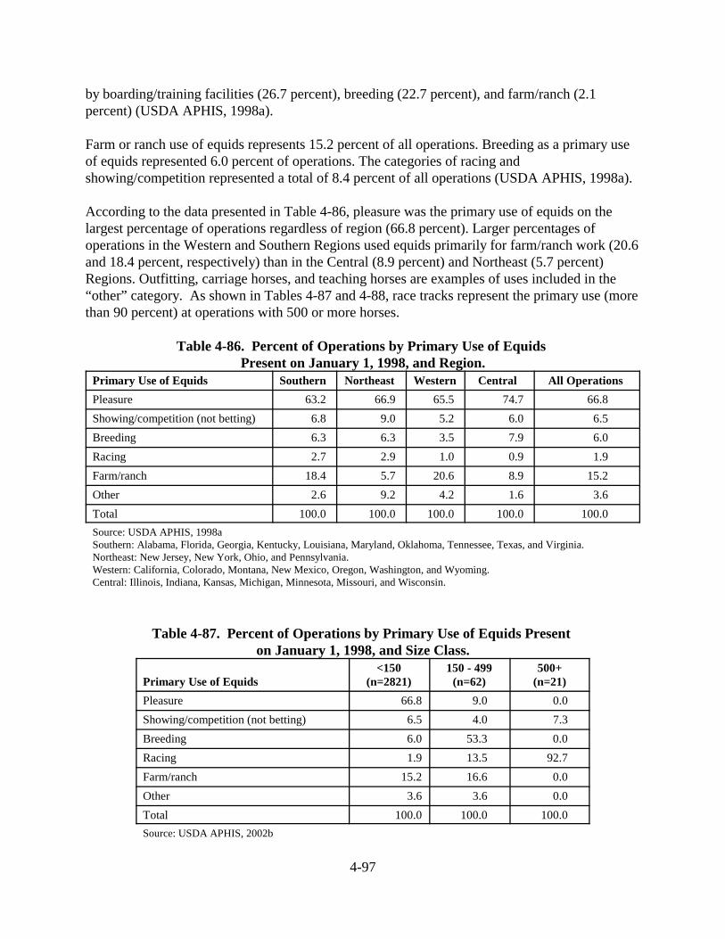
4-97

by boarding/training facilities (26.7 percent), breeding (22.7 percent), and farm/ranch (2.1percent) (USDA APHIS, 1998a).

Farm or ranch use of equids represents 15.2 percent of all operations. Breeding as a primary useof equids represented 6.0 percent of operations. The categories of racing andshowing/competition represented a total of 8.4 percent of all operations (USDA APHIS, 1998a).

According to the data presented in Table 4-86, pleasure was the primary use of equids on thelargest percentage of operations regardless of region (66.8 percent). Larger percentages ofoperations in the Western and Southern Regions used equids primarily for farm/ranch work (20.6and 18.4 percent, respectively) than in the Central (8.9 percent) and Northeast (5.7 percent)Regions. Outfitting, carriage horses, and teaching horses are examples of uses included in the“other” category. As shown in Tables 4-87 and 4-88, race tracks represent the primary use (morethan 90 percent) at operations with 500 or more horses.

Table 4-86. Percent of Operations by Primary Use of Equids Present on January 1, 1998, and Region.

Primary Use of Equids Southern Northeast Western Central All Operations

Pleasure 63.2 66.9 65.5 74.7 66.8

Showing/competition (not betting) 6.8 9.0 5.2 6.0 6.5

Breeding 6.3 6.3 3.5 7.9 6.0

Racing 2.7 2.9 1.0 0.9 1.9

Farm/ranch 18.4 5.7 20.6 8.9 15.2

Other 2.6 9.2 4.2 1.6 3.6

Total 100.0 100.0 100.0 100.0 100.0

Source: USDA APHIS, 1998aSouthern: Alabama, Florida, Georgia, Kentucky, Louisiana, Maryland, Oklahoma, Tennessee, Texas, and Virginia.Northeast: New Jersey, New York, Ohio, and Pennsylvania.Western: California, Colorado, Montana, New Mexico, Oregon, Washington, and Wyoming.Central: Illinois, Indiana, Kansas, Michigan, Minnesota, Missouri, and Wisconsin.

Table 4-87. Percent of Operations by Primary Use of Equids Present on January 1, 1998, and Size Class.

Primary Use of Equids <150

(n=2821)150 - 499

(n=62)500+

(n=21)

Pleasure 66.8 9.0 0.0

Showing/competition (not betting) 6.5 4.0 7.3

Breeding 6.0 53.3 0.0

Racing 1.9 13.5 92.7

Farm/ranch 15.2 16.6 0.0

Other 3.6 3.6 0.0

Total 100.0 100.0 100.0

Source: USDA APHIS, 2002b

4-98

Table 4-88. Percent of Operations by Primary Use of Equids Present on January 1, 1998, and Size Class.

Primary Function of Operation<150

(n=2821)150 - 499

(n=62)500+

(n=21)

Boarding/training 3.7 17.6 7.3

Racetrack 0.0 6.7 92.7

Breeding farm 5.1 53.6 0.0

Farm/ranch 32.7 17.0 0.0

Residence with equids for personal use 54.7 0.0 0.0

Other 3.8 5.1 0.0

Total 100 100 100

Source: USDA AHPIS, 2002.

4.5.2 Waste Management Practices

Nationally, stalls are provided on two-thirds of operations (does not include race tracks). NewEngland states provide stalls on 94.5 percent of their operations, while about one-half ofoperations in the western United States provide stalls. For those operations that do provide stalls,71.3 percent had at least one stall per equid. About one-third (34.5 percent) of those operationswith stalls clean them at least once a day, while 50.2 percent clean stalls once a week or lessoften. Straw, hay, wood shavings, chips, or sawdust are the most common type of bedding. Lessthan 40 (36.4) percent of operations indicate that they usually or sometimes compost manure orwaste bedding on site. For those operations with more than 20 equids, the most common methodof disposal was to apply the waste to fields where no animals graze (30.7 percent), followed byapplying it to fields where livestock graze (29.7 percent), allowing manure/waste bedding toaccumulate or leaving it to nature (15.1 percent), selling it or giving it away (11.5 percent), andhauling it away to someplace other than a landfill (8.9 percent) (USDA APHIS, 1998b).

Horse manure is usually handled as a solid. Many operations collect manure from stalls andpaddocks regularly. This is usually done with a fork or shovel and a wheelbarrow, tractor-loader,or trailer. Daily maintenance of horses in a confined setting requires intense labor requirementsto maintain sanitary conditions for the housed animals. Once manure and dirty bedding havebeen removed, wet areas might be treated with lime to maintain safe, clean, and odor-freeconditions (Wheeler and Cirelli, 1995). Fresh bedding, typically composed of such materials aspine sawdust, peanut shells, peatmoss, rice hulls, and other absorbent materials, is addedfollowing removal of manure and soiled bedding to ensure clean, dry conditions. Simply addingfresh bedding and allowing manure and soiled bedding to accumulate in the horse stall results indirty animals, provides excellent fly-breeding conditions, and may be unhealthy to horses(Graves, 1987). Depending on conditions, the runoff from paddocks, pens, corrals, and outdoorareas might need to be diverted to a settling basin or filter strip.

Manure management in pastures depends primarily on good distribution of manure across thepasture. Rotational grazing is a good option to avoid manure concentration in isolated spots in a

4-99

pasture. Additionally, avoiding grazing during rainy periods when soils are saturated isimportant to avoid soil compaction and manure runoff. Restricted access to streams avoidsmanure deposition in or near water bodies. Also, damaging the grass stand increases thepotential for manure runoff from pastures. The risk of this can be reduced by refraining fromexcessive stocking rates that lead to overgrazing (Colorado State University, 1996).

4.5.2.1 Waste Storage

Manure is typically stockpiled prior to use, providing greater flexibility for land application. TheGovernment of British Columbia (1998) recommends not to stockpile manure directly on theground for long-term storage where there is high rainfall or water tables. The size of any storagefacility would depend on the number of animals housed. A facility 12 feet wide by 12 feet longby 6 feet high can hold a year’s worth of manure for a 1,000-pound animal (USDA, 1997).

For horse operations that employ confined operations, an on-site storage facility is considered themost efficient way to collect and contain manure. Manure storage facilities should receive asmuch attention and planning as any other aspect of a horse operation (B.C. Government, 1998). Storage facilities are permanent structures designed and operated to contain all manure until itcan be applied as a fertilizer or removed for use elsewhere. Basic siting and sizingconsiderations of storage facilities from the B.C. Government (1998) include the following:

C Located at least 15 meters (50 feet) away from any watercourse and at least 30 meters (100 feet) away from wells or domestic water sources.

C Located so that clean surface runoff from adjacent areas is excluded.

C Sized to provide enough storage to prevent having to spread manure during the fall andwinter or at any time runoff is likely to occur.

C Of watertight construction.

C Structurally sound (with possible consideration of professionally engineered designs for bothearthen and concrete structures).

C Sized and located to contain all of the runoff expected from local climatic conditions, usingfigures from the worst precipitation in 25 years.

C Adequately fenced to prevent the accidental entry of humans, animals, or machinery.

C Located out of sight and downwind from public places and neighboring residences (wherepossible).

C Covered in areas of the province receiving more than 600 millimeters (24 inches) of rainfallbetween October and April.

4-100

4.5.2.2 Waste Treatment and Disposal

For smaller operations, composting is commonly used to treat horse manure. Compostingproduces a relatively dry end-product that is easily handled and reduces the volume of themanure (40 to 65 percent less volume and weight than the raw material). Ideal conditions forcomposting include a carbon-to-nitrogen (C:N) ratio between 25:1 and 30:1, a moisture contentbetween 40 and 60 percent, and good aeration. Horse manure as excreted has a C:N ratio of19:1. With the addition of bedding, the C:N ratio usually increases to a level ideal forcomposting. Under normal composting conditions, the internal temperature will increase tobetween 135 °F and 160 °F, killing most pathogens, parasites, and weed seed. Properlyconstructed and maintained compost piles or windrows will finish composting in as few as 90days, though the average time is approximately 120 days. When the composting process iscomplete, the temperature cools naturally.

Compost can be reused on horse pastures. However, experience has shown in the absence ofcareful management, this practice can spread internal parasites. Composted manure/bedding canalso be used as a surface for riding areas when mixed with sand and wood products. Shavings-based stall waste can often be used by nurseries and do not require a complete compostingprocess. Table 4-89 shows the average rates of horse manure application for forages and shouldfollow normal practices for minimizing runoff and leaching that are applicable for all manures.

Table 4-89. Average Manure Application Rates and Area Requirements for Forages.

ForageYield

(tons/acre) Horse Manure

(tons/acre)Land Base Needed

(acres/horse/yr)Alfalfa 4 30 0.3Alfalfa-Grass 4 20 0.4Bentgrass 2 21 0.4Big Bluestem 3 10 0.9Birdsfoot Trefoil 3 25 0.4Bluegrass 2 19 0.5Bromegrass 3 19 0.5Little Bluestem 3 11 0.8Orchard Grass 4 20 0.5Red Clover 3 20 0.4Reed Canary Grass 4 18 0.8RyeGrass 4 22 0.3Switchgrass 3 12 0.8Source: Colorado State University, 1996.

4-101

4.6 References

Abt. 1998. Preliminary study of the livestock and poultry industry: Appendices. Abt AssociatesInc., Cambridge, Massachusetts.

Adams, R. S., 1995. Dairy reference manual. 3rd ed. Northeast Regional AgriculturalEngineering Service Cooperative Extension

AAFC. (Agriculture and Agri-Food Canada), 1999. Farming for tomorrow: Conservation facts.Rotational grazing: The rest and recovery method of pasture management.<http://aceis.agr.ca/pfra/land/fft10.htm>. Accessed February 2000.

Aust, P. 1997. An institutional analysis of vertical coordination versus vertical integration: Thecase of the US broiler industry. Michigan State University, Department of AgriculturalEconomics, East Lansing, Michigan.

British Columbia Government. 1998. Manure Management Chapter 8, Horse Owner. Ministryof Agriculture and Food, Planning for Agriculture. British Columbia Government, Victoria, BC,Canada.

Bickert, W.G., G.R. Bodman, B.J. Holmes, D.W. Kammel, J.M. Zulovich, and R. Stowell. 1997.Dairy freestall housing and equipment. 6th ed. Midwest Plan Service, Agricultural andBiosystems Engineering Department

Bocher, L. W. 2000. Custom heifer grower, specialize in providing replacements for dairy herds,Hoard’s Dairyman

Bodman, G.R., D.W. Johnson, D.G. Jedele, V.M. Meyer, J.P. Murphy, and H.L. Person. 1987.Beef housing and equipment handbook. 4th ed. Midwest Plan Service.

Bradley, F., D. Bell, R. Ernst, D. McMartin, and J. Milliam. 1998. Animal care series: Egg-typelayer flock care practices. California Poultry Workgroup, University of CaliforniaCooperative Extension, University of California Publishing, Davis, California.

British Columbia Government. 1998. Manure Management. Chapter 8, Horse Owner. Ministryof Agriculture and Food, Planning for Agriculture. British Columbia Government.

Brodie, H.L. Carr, and C. Miller. 2000. Structures for broiler litter manure storage.<http://www.hermes.ecn.purdue.edu/cgi/convertwq?5343>. Accessed November 2000.

Cady, Roger. Personal communication, Monsanto Company and Founder of the ProfessionalDairy Heifer Growers Association. Personal communication, February 18, 2000.

4-102

CIAS. 2000a. Grazing’s potential: Predicting expansion’s cost, profit. Center for IntegratedAgricultural Systems, <http://www.wisc.edu/cias/pubs/resbrief/030.html>. Accessed May2000.

CIAS. 2000b. Outwintering dairy cattle: Animal health issues. Center for Integrated AgriculturalSystems, <http://www.wisc.edu/cias/pubs/resbrief/027.html>. Accessed May 2000.

CIAS. 2000c. Outwintering dairy cattle: Manure management issues. Center for IntegratedAgricultural Systems, <http://www.wisc.edu/cias/pubs/resbrief/028.html>, Accessed May2000.

CIAS. 2000d. Dairy grazing can provide good financial return. Center for IntegratedAgricultural Systems, <http://www.wisc.edu/cias/pubs/resbrief/050.html>. Accessed May2000.

Colorado State University. 1996. Management of Horse Manure: A Renewable Resource. Colorado State University Cooperative Extension, Fort Collins, CO. December 1996.

Dougherty, M., L.D. Geohring, and P. Wright. 1998. Liquid manure application systems,Northeast Regional Agricultural Engineering Service, NRAES-89.

Emmicx, D.L. 2000. ABC’s of rotational grazing: Questions and answers.<http://www.kingcd.org/stewardship/Ag%20Pr...ces/Pastures/ABCsofRotationalGrazing.html>. Accessed February, 2000.

ERG. 2000a. Stand alone dairy heifer raising operations. Memorandum from Birute Vanatta,Eastern Research Group, Inc. to Ron Jordan, U.S. Environmental Protection Agency.

ERG. 2000b. Facility counts for beef, dairy, veal, and heifer operations. Memorandum from DebBartram, Eastern Research Group, Inc., to the Feedlots Rulemaking Record.

Faust, M.A. 2000. Dairy replacement heifer enterprises. <Web address>. Accessed February 14,2000.

Gardner, Don. South East District Director for the Professional Dairy Heifer GrowersAssociation. Personal communication, December 9, 1999.

Goan, C. 2000. Storage facilities for broiler litter. <http://hermes.ecn.purdue.edu/cgi/convertwq?7146>. Accessed November 20, 2000.

Graves, R.E. 1987. Animal Manure – Manure Management for Horses. PENpages Number: 0870177. Pennsylvania State University Agricultural Engineering Department.

Hamm, D., G. Searcy, and A. Mercuri. 1974. A study of the waste wash water from egg washingmachines. Poultry Science 53:191-197.

4-103

Hannawald, Jim. U.S. Department of Agriculture. Personal communication, April 4, 2000.

Hansen, D. 2000. State regulatory issues and implications: Eastern USA, in Proceedings: 2000National Poultry Waste Management Symposium, Ocean City, Maryland.

Hutchinson, L.J. 1988. Animal health, pest management and environment. In Proceedings ofPasture in the Northeast Region of the United States. U.S. Department of Agriculture, SoilConservation Service, Northeast National Technical Center, Chester, Pennsylvania.

Jordan, Larry. South East Regional Director for the Professional Dairy Heifer GrowersAssociation. Personal communication, December 8, 1999.

Kellog, R. 2002. Profile of Farms with Livestock in the United States: A Statistical Summary; R.Kellogg; Feb 4, 2002; 31 pages.

Kellogg, R.L., C. Lander, D. Moffitt, and N. Gollehon. Manure nutrients relative to the capacityof cropland and pastureland to assimilate nutrients: Spatial and temporal trends for theU.S. April 27, 2000.

Loudon, T.L., D.D. Jones, J.B. Petersen, L.F. Backer, M.F. Brugger, J.C. Converse, C.D.Fulhage, J.A. Lindley, S.W. Nelvin, H.L. Person, D.D. Schulte, and R. White. 1985.Livestock waste facilities handbook. 2nd ed. Midwest Plan Service.

Maple Leaf Farms. 2001. Facility Distribution data gathered by Maple Leaf Farms; prepared byDan Harper; June 29, 2001.

Martinez, S.W. 1999. Vertical coordination in the pork and broiler industries: Implications forpork and chicken products. Agriculture Economic Report No. 777. U.S. Department ofAgriculture, Economic Research Service, Food and Rural Economics Division, Washington,DC.

Meyer, D. J. 1987. Animal manure–Veal calf management. <http://www.inform.umd.edu:8080/EdRes/topic/AgrEnv/ndd/watermgt/ANIMAL_MANURE_VEAL_CALF_MANAGEM.html>.

Moats, W.A. 1978. Factors Affecting Bacterial Loads on Shells of Commercially Washed Eggs.Poultry Science 60:2084-2090.

Murphy, B. 1988. Voisin grazing management in the Northeast. In Proceedings of Pasture in theNortheast Region of the United States. U.S. Department of Agriculture, Soil ConservationService, Northeast National Technical Center, Chester, Pennsylvania.

NCBA. 1999. Comments on the draft industry profile. National Cattlemen’s Beef Association.

4-104

NCC. 1999. Comments on EPA profile of broiler industry. National Chicken Council,Washington, DC.

National Milk Producers Federation submittal to U.S. Environmental Protection Agency on3/1/99: State Level Milk Production.

NCSU. 1998a. Draft of swine and poultry industry characterization, waste managementpractices and modeled detailed analysis of predominantly used systems. North Carolina StateUniversity.

NCSU. 1998b. Nutritional strategies to reduce swine and poultry waste quantity and N and P inwaste. North Carolina State University.

Noyes, T.E. 1999. Heifer raising conference. December 3, 1999. <http://www.ag.ohio-state.edu/~wayn/dairy/darnews.htm> Assessed.December 3, 1999.

NPPC. 1996. Swine care handbook. (National Pork Producers Council),<http://nppc.org/prod/swinecarehandbook.html>. Accessed August 17, 1999.

NPPC. 1998. Environmental assurance program survey.

NPPC. 1999. Pork facts 1998/99. (National Pork Producers Council),<http://nppc.org/prod/swinecarehandbook.html>. Accessed August 15, 1999.

NRC. 1989. Nutrient requirements of dairy cattle, 6th rev. ed. National Research Council.

PPRC. 1996. Impacts of intensive rotational grazing on stream ecology and water quality.Pacific Northwest Pollution Prevention Resource Center,<http://www.pprc.org/pprc/rpd/fedfund/usda/sare_nc/impactsi.html>. Accessed February,2000.

PADER. 1986. Swine manure management. Pennsylvania Department of EnvironmentalResources, Harrisburg, Pennsylvania.

Rasby, R., I. Rush, and R. Stock. 1996. Wintering and backgrounding beef calves.<http://www.ianr.unl.edu/PUBS/BEEF/g1228.htm>.

Scott, M.L. and W.F. Dean. 1991. Nutrition and Management of Ducks. M.L. Scott of Ithaca,Ithaca, NY.

Stull, C.E., S. Berry, and E. DePeters. 1998. Animal care series: Dairy care practices. 2nd ed.Dairy Workgroup, University of California Cooperative Extension.

Sweeten, J. n.d. Manure management for cattle feedlots. Great Plains Beef Cattle Handbook.Cooperative Extension Service - Great Plains States.

4-105

Thompson, G.B. and C.C. O’Mary. 1983. The feedlot. 3rd ed. Lea & Febiger, Philadelphia,Pennsylvania.

Thorne, J. 1999. Proposed EPA Project XL: United egg producers. Capitolink LLC, Washington,DC.

Tyson, T. 1996. Planning and managing lagoons for poultry layer waste treatment. AlabamaCooperative Extension Service, Auburn, Alabama.

UCD. 1998. Egg type- Layer flock care practices. California Poultry Workgroup, University ofCalifornia at Davis, Davis, California.

UEP. 1998. UEP (Egg Producers) Data Package. United Egg Producers. Submitted to USEPA.

USDA. (U.S. Department of Agriculture), Safety of veal, from Farm to table. <http://www.fsis.usda.gov/oa/pubs/veal/htm>. Accessed April 14, 1999.

USDA. 1997. Horses: A Common Sense Approach. U.S. Department of Agriculture. Spring.1997.

USDA. 1997. Chapter 5: Management of grazing lands. In National range and pasturehandbook. U.S. Department of Agriculture.

USDA APHIS. 1993. National Dairy Heifer Evaluation Project, Contract heifer raising. U.S.Department of Agriculture, Animal and Plant Health Inspection Service, Fort Collins,Colorado.

USDA APHIS. 1995. Swine ’95 Part 1: Reference of 1995 swine management practices. U.S.Department of Agriculture, Animal and Plant Health Inspection Service, Fort Collins,Colorado.

USDA APHIS. 1996a. National Animal Health Monitoring System, Part I: Reference of 1996dairy management practices. U.S. Department of Agriculture, Animal and Plant HealthInspection Service, Fort Collins, Colorado.

USDA APHIS. 1996b. National Animal Health Monitoring System, Part III: Reference of 1996dairy health and health management. U.S. Department of Agriculture, Animal and PlantHealth Inspection Service, Fort Collins, Colorado.

USDA APHIS. 1996c. Swine ’95 Part II: Reference of 1995 grower/finisher health andmanagement. U.S. Department of Agriculture, Animal and Plant Health Inspection Service.Fort Collins, Colorado.

4-106

USDA APHIS. 1996d. The USDA’s Role in Equine Health Monitoring.<http://www.aphis.usda.gov/vs/ceah/cahm/>. U.S. Department of Agriculture, Animal andPlant Health Inspection Service.

USDA APHIS. 1998a. National Animal Health Monitoring System, Part I: Baseline Reference of1998 Equine Health and Management. <http://www.aphis.usda.gov/vs/ceah/cahm/>. Fileeq98pt1.pdf accessed October 15, 1998. U.S. Department of Agriculture, Animal and PlantHealth Inspection Service.

USDA APHIS. 1998b. National Animal Health Monitoring System, Part II: Baseline Referenceof 1998 Equine Health and Management. <http://www.aphis.usda.gov/vs/ceah/cahm/>. Fileeq98pt2.pdf accessed October 15, 1998. U.S. Department of Agriculture, Animal and PlantHealth Inspection Service.

USDA APHIS. 1999. Swine ’95 Reference of 1995 swine management practices. Additionaldata queries run at the request of EPA for new region and size categories. U.S. Department ofAgriculture, Animal and Plant Health Inspection Service, Fort Collins, Colorado.

USDA APHIS. 2000a. National Animal Health Monitoring System, Part I: Baseline reference offeedlot management practices. U.S. Department of Agriculture, Animal and Plant HealthInspection Service, Fort Collins, Colorado.

USDA APHIS. 2000b. Part II: Reference of 1999 table egg layer management in the UnitedStates (Layer ’99). U.S. Department of Agriculture, Animal Plant Health Inspection Service,Fort Collins, Colorado.

USDA APHIS. 2001. Part I: Reference of Swine Health and Management in the United States,2000, United State Department of Agriculture National Animal Health Monitoring System,Fort Collins, Colorado.

USDA APHIS. 2002a. Queries run by Centers for Epidemiology and Animal Health prepared byEric Bush; March 22, 2002; 2 pages. Centers for Epidemiology and Animal Health. U.S.Department of Agriculture (USDA), Animal Plant Health Inspection Service (APHIS),National Animal Health Monitoring System, Fort Collins, Colorado.

USDA AHPIS. 2002b. Data aggregated from Equine ‘‘98 data by Michael Durham, Centers forEpidemiology and Animal Health. U.S. Department of Agriculture (USDA), Animal PlantHealth Inspection Service (APHIS), National Animal Health Monitoring System, FortCollins, Colorado.

USDA BAMN. 1997. A guide to dairy calf feeding and management. U.S. Department ofAgriculture (USDA), Bovine Alliance on Management & Nutrition (BAMN)<http://www.aphis.usda.gov/vs/ceah/cahm/ File bamnfeed.htm>. Accessed

4-107

USDA ERS. 1997. The U.S. Pork industry: As it changes, consumers stand to benefits U.S.Department of Agriculture, Economic Research Service, Washington, DC.

USDA NAHMS. 1999. Data aggregated from Swine ‘95 data, U.S. Department of Agriculture,Animal Plant Health Inspection Service, National Animal Health Monitoring System, Centersfor Epidemiology and Animal Health. Fort Collins, Colorado.

USDA NAHMS. 2000. Data Aggregated from Layer 99 data by Lindsey Garber, U.S.Department of Agriculture, Animal Plant Health Inspection Service, National Animal HealthMonitoring System (NAHMS). Centers for Epidemiology and Animal Health. Fort Collins,Colorado.

USDA NASS. 1995a. Milk: Final estimates 1988-1992. Statistical Bulletin 909. U.S.Department of Agriculture (USDA), National Agricultural Statistics Service, Washington,DC.

USDA NASS. 1998a. Agricultural statistics. U.S. Department of Agriculture, NationalAgricultural Statistics Service, Washington, DC.

USDA NASS. 1998b. Chickens and eggs final estimates 1994-97. Statistical Bulletin No. 944.U.S. Department of Agriculture, National Agricultural Statistics Service, Washington, DC.

USDA NASS. 1998c. Poultry production and value, final estimates 1994-97. Statistical BulletinNo. 958. U.S. Department of Agriculture, National Agricultural Statistics Service,Washington, DC.

USDA NASS. 1999a. Hogs and Pigs: Final estimates 1993-1997. Statistical Bulletin Number951. U.S. Department of Agriculture, National Agricultural Statistics Service, Washington,DC.

USDA NASS. 1999b. 1997 census of agriculture. U.S. Department of Agriculture, NationalAgricultural Statistics Service, Washington, DC.

USDA NASS. 1999c. Queries run by NASS for USEPA on the 1997 Census of Agriculture data.U.S. Department of Agriculture, National Agricultural Statistics Service, Washington, DC.

USDA NASS. 1999d. Milking cows and production: Final estimates 1993-1997. StatisticalBulletin 952. U.S. Department of Agriculture, National Agricultural Statistics Service,Washington, DC.

USDA NASS. 1999e. Cattle: Final estimates 1994-1998. Statistical Bulletin 953. U.S.Department of Agriculture, National Agricultural Statistics Service, Washington, DC.

4-108

USDA NRCS. 1992. Agricultural waste management field handbook, National engineeringhandbook (NEH), Part 651. U.S. Department of Agriculture, Natural Resources ConservationService, Washington, DC.

USDA NRCS. 1996. Dairy farmer profitability using intensive rotational stocking: Bettergrazing management for pastures. U.S. Department of Agriculture, Natural ResourcesConservation Service, Grazing Lands Technology Institute. Washington, DC.

USDA NRCS. 1998. Nutrients available from livestock manure relative to crop growthrequirements. U.S. Department of Agriculture, Natural Resources Conservation Service,Washington, DC.

USEPA. 1998. Feedlot industry sector profile. Revised draft report. Prepared for U.S.Environmental Protection Agency by Tetra Tech, Inc., Fairfax, Virginia.

Vest, L. n.d. Layer production. Georgia Farm*A*Syst. Cooperative Extension Service,University of Georgia, College of Agricultural and Environmental Sciences. Athens, Georgia.

Wheeler, Gene, and A. Cirelli. 1995. Animal Waste Management for the Horseowner. Fact Sheet95-11, University of Nevada Cooperative Extension, Lincoln, Nebraska.

Wilson, L.L., C.L. Stull, and T.L. Terosky. 2000. Scientific advancements and legislationaddressing veal calves in North America. In: Veal Perspectives to the Year 2000,Proceedings of an International Symposium, LeMans, France, September 12 and 13, 1995,LeMans, France.

development document for the final revisions to the national

Documents