development and utilization of integrated artificial

The Pennsylvania State University

The Graduate School

John and Willie Leone Family Department of Energy and Mineral Engineering

DEVELOPMENT AND UTILIZATION OF INTEGRATED

ARTIFICIAL EXPERT SYSTEMS FOR DESIGNING MULTI-

LATERAL WELL CONFIGURATIONS, ESTIMATING

RESERVOIR PROPERTIES AND FORECASTING RESERVOIR

PERFORMANCE

A Dissertation in

Energy and Mineral Engineering

by

Talal Saeed Almousa

© 2013 Talal Saeed Almousa

Submitted in Partial Fulfillment

of the Requirements

for the Degree of

Doctor of Philosophy

August 2013

ii

The dissertation of Talal Saeed Almousa was reviewed and approved* by the following:

Turgay Ertekin

Head of the John and Willie Leone Family Department of Energy and Mineral Engineering

George E. Trimble Chair in Earth and Mineral Sciences

Professor of Petroleum and Natural Gas Engineering

Dissertation Adviser and Chair of Committee

Mirna Urquidi-Macdonald

Professor Emeritus of Engineering Sciences and Mechanics

Li Li

Assistant Professor of Petroleum and Natural Gas Engineering

Michael Adewumi


Vice Provost for Global Programs

Turgay Ertekin

Head of the John and Willie Leone Family Department of Energy and Mineral Engineering

George E. Trimble Chair in Earth and Mineral Sciences


*Signatures are on file in the Graduate School.

iii

Abstract

Reservoir simulation is one of the main tools if not the most important one reservoir

engineers use to forecast a reservoir performance. Nevertheless, developing and operating a

reservoir simulator in the first place can be an arduous task that requires a set of highly skilled

individuals in science, advanced mathematics, programing, and reservoir engineering and

powerful computational models.

The reliability of a reservoir simulator depends on the availability and the quality of the

reservoir properties. These properties are obtained from open-hole logs, core studies and well

testing analysis which can sometimes be prohibitively cost intensive.

Another important component of the overall process affecting the reservoir performance

is the multilateral well configuration. Achieving the right design of a multilateral well

configuration is a complex problem due to the vast possibilities of well forms that need to be

evaluated.

In light of the above, this dissertation demonstrates the development and the application

of a set of integrated artificial expert systems in the area of forecasting, reservoir evaluation and

multilateral well design. The applied method has gradually progressed in degrees of complexity

from addressing a preliminary case of volumetric single phase gas reservoirs completed with

only dual-laterals towards an expanded form of the same system with varying multi-laterals and

reservoir properties to eventually and successfully implementing it to multiphase reservoirs with

bottom water drive systems completed with multi-laterals (choice of 2-5 laterals). The developed

method and tools cover a wide spectrum of rock and fluid properties spanning tight to

conventional sands. The developed approach successfully delivers a total of five distinct artificial

iv

expert systems, three of them serve as proxies to the conventional numerical simulator for

predicting reservoir performance in terms of cumulative oil recovery, cumulative oil and gas

productions and estimating the end of plateau and abandonment times and a third one for

predicting cumulative fluid production. These aforementioned systems are categorized as

forward-looking solutions. Whereas the other two artificial expert systems are categorized as

inverse-looking solutions, one that addresses the multi-lateral well design problem and the other

that estimates critical reservoir properties that can be used at the very least as first estimators in

assist history matching problems and for improving the assessment of nearby prospects in field

development or in-fill drilling exercises.

Furthermore, graphical user interfaces (GUIs) in conjunction with the expert systems

structured are developed and assembled together for standalone installation. These GUIs allow

the engineer to edit and input data, produce results numerically and graphically, compare results

with a commercial numerical simulator, and generate an interactive 3-D visualization of the

multilateral well.

It is expected that the developed integrated artificial expert systems will immensely

reduce expenses and time requirements and effectively enhance the overall decision-making

process. However, it is worth noting that the proposed expert systems are not to replace the

conventional and well established procedures and protocols but rather as auxiliary or

complementary applications, where applicable, to relief some of the computational overhead,

provide educated estimation of key reservoir properties or the very least help fine tune them and

present the inverse-looking solution to the multi-lateral well design problem or the least a

starting point.

v

Table of Contents

List of Figures .............................................................................................................................. vii

List of Tables .............................................................................................................................. xiii

Acknowledgements .................................................................................................................... xiv

Chapter 1 Introduction................................................................................................................. 1

Chapter 2 Literature Review ....................................................................................................... 5

2.1 Artificial Neural Network ...................................................................................................... 5

2.2 Petroleum Engineering Applications of Artificial Expert Systems ..................................... 13

2.3 Relevant Studies .................................................................................................................. 16

Chapter 3 Problem Statement ................................................................................................... 18

Chapter 4 Methodology .............................................................................................................. 22

4.1 Feasibility Study .................................................................................................................. 22

4.2 Data Base Generation ......................................................................................................... 22

4.3 Artificial Neural Network Design Workflow ....................................................................... 25

Chapter 5 Feasibility Study........................................................................................................ 28

5.1 Preliminary Case Description ............................................................................................. 28

5.2 Approach ............................................................................................................................. 30

5.3 Data Base Generation ......................................................................................................... 32

5.4 Forward-Looking ANN ....................................................................................................... 36

5.5 Inverse-Looking ANN .......................................................................................................... 51

5.6 Summary and Lessons Learned ........................................................................................... 77

Chapter 6 Developed Expert Systems for Volumetric Single Phase Gas Reservoirs ........... 79

6.1 Forecast Expert System (FExS) Development for Volumetric Single Phase Gas Reservoirs

(VSPGR) .................................................................................................................................... 79

6.2 Multi-Lateral Well Design Advisory System (MLWDAS) Development for Volumetric

Single Phase Gas Reservoirs .................................................................................................... 86

vi

6.3 Reservoir Evaluation Expert System (REExS) Development for Volumetric Single Phase

Gas Reservoirs (VSPGR) .......................................................................................................... 96

Chapter 7 Developed Expert Systems for Multi-Phase Reservoirs with Bottom Water Drive

..................................................................................................................................................... 113

7.1 Definition of Parameters ................................................................................................... 114

7.2 Forecast Expert System (FExS) Development for Multi-Phase Reservoirs with Bottom

Water Drive (MPRBWD) ........................................................................................................ 117

7.3 Multi-Lateral Well Design Advisory System (MLWDAS) Development for Multi-Phase

Reservoirs with Bottom Water Drive (MPRBWD) .................................................................. 121

7.4 Reservoir Evaluation Expert System (REExS) Development for Multi-Phase Reservoirs

with Bottom Water Drive (MPRBWD) .................................................................................... 129

7.5 Cumulative Fluid Production Expert System (CFPExS) Development ............................ 133

7.6 Cumulative, Abandonment and Plateau Times Expert System (CAPTExS) Development 138

Chapter 8 Graphical User Interface and Summary .............................................................. 144

8.1 Integrated Artificial Expert Systems Graphical User Interfaces (GUIs) .......................... 144

8.2 Summary ............................................................................................................................ 153

8.3 Recommendations.............................................................................................................. 154

References .................................................................................................................................. 155

Appendix A ................................................................................................................................ 158

Sample Data Files ................................................................................................................... 158

A.1 Sample Data File for Volumetric Single Phase Gas Reservoirs ...................................... 158

A.2 Sample Data File for Multi-Phase Reservoirs With Bottom Water Drive ........................ 161

vii

List of Figures

Fig. ‎2.1: Interconnection of biological neural networks (Graupe, 2007)........................................ 6

Fig. ‎2.2: A simple abstract of an ANN from a biological nerve (Nelson, 2012). ........................... 7

Fig. ‎2.3: A typical ANN architecture (Chidambaram, 2009). ........................................................ 9

Fig. ‎2.4: A Neuron Model (Demuth & Beale, 2002). ................................................................... 10

Fig. ‎2.5: Graphical Representations of the Most Common Transfer Functions (Demuth & Beale,

2002). ..................................................................................................................................... 11

Fig. ‎4.1: Data Base Preparation Flow Chart. ................................................................................ 25

Fig. ‎5.1: 3D Model Schematics..................................................................................................... 28

Fig. ‎5.2: Top View of the Model. ................................................................................................. 29

Fig. ‎5.3: Preliminary Case Study Flow Chart. .............................................................................. 32

Fig. ‎5.4: ANN Architecture for the Initial Forward-Looking solution. ........................................ 44

Fig. ‎5.5: Regression Plots for the Forward-Looking ANN solution of Fig. 5.4. .......................... 45

Fig. ‎5.6: Recovery Profile Predictions, ANN vs. Simulator, (best & worst match). .................... 46

Fig. ‎5.7: The Remaining Comparison Plots for the Test set. ........................................................ 47

Fig. ‎5.8: Expanded Forward-Looking Network #18 Architecture. ............................................... 50

Fig. ‎5.9: Comparison Plots of the Recovery Profile Predictions (ANN vs. Simulator). .............. 51

Fig. ‎5.10: ANN Architecture for the Initial Inverse-Looking solution. ........................................ 53

Fig. ‎5.11: Regression Plots for the Initial Inverse-Looking ANN solution of Fig. 5.10. ............. 54

Fig. ‎5.12: Comparison Plots of Two Parameters for all Test Cases (ANN vs. Target). ............... 55

Fig. ‎5.13: The Remaining Parameters Comparison Plots for all Test Cases. ............................... 56

Fig. ‎5.14: ANN Architecture for the Expanded Inverse-Looking solution. ................................. 57

Fig. ‎5.15: Parameters Comparison Plots of for all Test Cases (ANN vs. Target). ....................... 58

viii

Fig. ‎5.16: Regression Plots for the Expanded Inverse-Looking ANN solution of Fig. 5.14. ....... 59

Fig. ‎5.17: Testing the Expanded Inverse-Looking Solution with 18 New Data Sets (ANN vs.

Target). .................................................................................................................................. 61

Fig. ‎5.18: Results from Three Modified Inverse-Looking ANNs (ANN vs. Target). .................. 64

Fig. ‎5.19: Error Plots of Each Parameter/Network and the Total Average Error/Network. ......... 65

Fig. ‎5.20: Each Parameter Average Error of the 26 cases for All the Networks and for Network

19. .......................................................................................................................................... 66

Fig. ‎5.21: Crosschecking Process of the Modified Inverse-Looking ANNs Using a Numerical

Simulator. .............................................................................................................................. 69

Fig. ‎5.22: Modified Inverse-Looking Network #19 Architecture. ................................................ 70

Fig. ‎5.23: Crosschecking Process of the Modified Inverse-Looking ANNs Using the Expanded

Forward-Looking ANN Solution Network #18..................................................................... 72

Fig. ‎5.24: Parameters Predicted by the Inverse-Looking Network #19 for 9 Cases and Compared

With Targets. ......................................................................................................................... 74

Fig. ‎5.25: The Overall Average Error between Both Crosschecking Methods In Addition To the

Error between Both Tools...................................................................................................... 75

Fig. ‎5.26: Comparison Plots of the Recovery Profiles Predicted by Both Methods vs. the Targets

for 9 Cases. ............................................................................................................................ 76

Fig. ‎6.1: FExS Implemented to Volumetric Single Phase Gas Reservoirs (VSPGR). ................. 83

Fig. ‎6.2: FExS Results and Their Respective Errors Implemented to VSPGR . .......................... 84

Fig. ‎6.3: Comparison Plots Between the Recovery Profiles Predicted by FExS and the Simulator

(Target) Implemented to VSPGR. ......................................................................................... 85

Fig. ‎6.4: MLWDAS Implemented to VSPGR. ............................................................................. 87

ix

Fig. ‎6.5: Crosschecking Process for MLWDAS Using the Numerical Simulator. ....................... 88

Fig. ‎6.6: MLWDAS Results and Their Respective Errors Implemented to VSGRs. ................... 89

Fig. ‎6.7: Crosschecking Process for MLWDAS Using FExS. ..................................................... 91

Fig. ‎6.8: FExS vs. Target 84 Cases Distribution with Respect to their Ranges of error

Implemented to VSPGR. ....................................................................................................... 92

Fig. ‎6.9: FExS vs. Simulator 82 Cases Distribution with Respect to their Ranges of error


Fig. ‎6.10: Recovery Profiles Predicted by Both Crosschecking Methods for MLWDAS


Fig. ‎6.11: General Theme of the Expert Systems Development Progression. .............................. 97

Fig. ‎6.12: REExS Implemented to VSPGR. ................................................................................. 99

Fig. ‎6.13: REExS Testing Results on 10 Cases Implemented to VSPGR.. ................................ 100

Fig. ‎6.14: RDExS Implemented to VSPGR. ............................................................................... 103

Fig. ‎6.15: RDExS vs. Simulator 48 Cases Distribution with Respect to Their Ranges of error

Implemented to VSPGR. ..................................................................................................... 104

Fig. ‎6.16: Crosschecking Process for REExS Using the Numerical Simulator. ......................... 105

Fig. ‎6.17: Cases Distribution with Respect to their Ranges of Error when Comparing Observed

Rates to Simulator Rates Using REExS Predictions Implemented to VSPGR. .................. 107

Fig. ‎6.18: Crosschecking Process for REExS Using RDExS. .................................................... 108

Fig. ‎6.19: Cases Distribution with Respect to their Ranges of Error when Comparing Observed

Rates to RDExS Rates Using REExS Predictions Implemented to VSPGR. ...................... 109

Fig. ‎6.20: Rate Declines Predicted by Both Crosschecking Methods Using the REExS Inputs

Implemented to VSPGR. ..................................................................................................... 111

x

Fig. ‎6.21: Rate Declines Predicted by Both Crosschecking Methods Using the REExS Inputs. 112

Fig. ‎7.1: FExS Implemented to (MPRBWD).............................................................................. 118

Fig. ‎7.2: FExS Results and Their Respective Errors Implemented to MPRBWD. .................... 119

Fig. ‎7.3: Comparison Plots Between the Recovery Profiles Predicted by FExS and the Simulator

(Target) Implemented to MPRBWD. .................................................................................. 120

Fig. ‎7.4: MLWDAS Implemented to MPRBWD. ...................................................................... 122

Fig. 7.5: Target vs. Simulator of 88 Cases According to their Ranges of Error Implemented to

MPRBWD. .......................................................................................................................... 123

Fig. 7.6: Comparison Plots Between Target Recovery Profiles and Reproduced Profiles using

the Numerical Simulator Implemented to MPRBWD. ........................................................ 124

Fig. 7.7: Target vs. FExS of 88 Cases According to their Ranges of Error Implemented to

MPRBWD. .......................................................................................................................... 125

Fig. 7.8: Comparison Plots Between Target Recovery Profiles and Reproduced Profiles using

FExS Implemented to MPRBWD. ...................................................................................... 126

Fig. 7.9: The Overall Average Errors Between All Methods Implemented to MPRBWD. ...... 127

Fig. 7.10: Comparison Plots of Recovery Profiles Obtained by All Methods Implemented to

MPRBWD. .......................................................................................................................... 128

Fig. 7.11: REExS Implemented to MPRBWD. ......................................................................... 130

Fig. 7.12: Target vs. Simulator of 85 Cases According to their Ranges of Error Implemented to

MPRBWD. .......................................................................................................................... 131

Fig. 7.13: Comparison Plots Between Target Cumulative Fluid Production Profiles and

Reproduced Profiles using Numerical Simulator using REExS Predicted Reservoir

Properties Implemented to MPRBWD. ............................................................................... 132

xi

Fig. 7.14: CFPExS Implemented to (MPRBWD). ..................................................................... 134

Fig. 7.15: Target vs. CFPExS of 89 Cases According to their Ranges of Error Implemented to

MPRBWD. .......................................................................................................................... 134

Fig. 7.16: Comparison Plots Between Target and CFPExS Cumulative Fluid Production Profiles

Implemented to MPRBWD. ................................................................................................ 135

Fig. 7.17: Target vs. CFPExS of 85 Cases According to their Ranges of Error Implemented to

MPRBWD. .......................................................................................................................... 136

Fig. 7.18: Comparison Plots Between REExS Targets and CFPExS Cumulative Fluid Production

Profiles Implemented to MPRBWD. ................................................................................... 137

Fig. 7.19: CFPExS Implemented to (MPRBWD). ..................................................................... 138

Fig. 7.20: CAPTExS Results and Their Respective Errors Implemented to MPRBWD. ......... 140

Fig. 7.21: Comparison Plots of the CAPTExS_Np, Plateau and Abandonment Times versus their

respective Targets Implemented to MPRBWD. .................................................................. 141

Fig. ‎7.22: CAPTExS Results and Their Respective Errors Implemented to MPRBWD. .......... 142

Fig. ‎7.23: Comparison Plots of the CAPTExS_Gp vs. Target_Gp Implemented to MPRBWD.

............................................................................................................................................. 143

Fig. 8.1: Main Window of the Integrated Artificial Expert System Graphical User Interface

(GUI). .................................................................................................................................. 145

Fig. 8.2: Main Window of the Volumetric Single Phase Gas Reservoirs Expert System. ........ 146

Fig. 8.3: Reservoir Evaluation Expert System (REExS) GUI under VSPGR Environment. .... 148

Fig. 8.4: REExS GUI Illustrating Some of its Produced Results............................................... 148

Fig. 8.5: Forecast Expert System (FExS) GUI under VSPGR Environment............................. 149

xii

Fig. 8.6: Multi-Lateral Well Design Advisory System (MLWDAS) GUI under VSPGR

Environment. ....................................................................................................................... 150

Fig. 8.7: MLWDAS GUI Showing the Well Design Parameters and the 3D View. ................. 151

Fig. 8.8: MLWDAS GUI Showing the SIM and the FExS Predictions vs. the Target Cumulative

Percent Recoveries and Corresponding Errors. ................................................................... 152

xiii

List of Tables

Table ‎2.1: Transfer Functions (reproduced from (Chidambaram, 2009)) .................................... 12

Table ‎5.1: Parameters and their ranges ......................................................................................... 30

Table ‎5.2: Pseudorandom Parameters ........................................................................................... 33

Table ‎5.3: Constant Reservoir Properties and Operating Parameters ........................................... 36

Table ‎5.4: Cumulative Recovery Factors Produced by the Numerical Simulator ........................ 38

Table ‎5.5: Expanded Forward-Looking ANN Input Parameters and their ranges ....................... 48

Table ‎6.1: Reservoir, Well Design and Operating Parameters and Their Ranges ........................ 80

Table ‎7.1: Reservoir, Well Design and Operating Parameters and Their Ranges ...................... 115

xiv

Acknowledgements

I thank GOD Almighty for his countless blessings upon me and for giving me the well

and determination to complete this work. I am forever indebted to my loving parents, my lovely

mother Aisha and my wonderful father Saeed, for their never-ending care and nurture. I also

extend my appreciation and sincere thanks to my beautiful wife, Fatimah, for her endless love,

care and support.

I thank my Country’s government, Saudi Arabia, represented by the Custodian of the

Two Holly Mosques, King Abdullah bin Abdulaziz whom in his era, has revolutionized and

reshaped the kingdoms education by establishing many local public universities, institutions and

over one hundred thousand, to the date of this document, out of kingdom scholarships to USA,

Europe, Australia and East Asia. I extend my thanks and gratitude to my employer, at the time of

this study, Saudi Aramco for their direct financial liability and logistics support.

No words can express my sincere appreciation and pleasure for the four years that have

brought me closer to my adviser, my mentor and my dear friend Professor Tugay Ertekin. Whom

his commitment to his students and humbleness have amazed me, his knowledge and expertise

have inspired me and his teaching, work ethics and high standards have been sources of my

admiration.

I am also grateful for the services of my committee members and for their wise

comments and recommendations represented by Professor Mirna Urquidi-Macdonald, Professor

Michael Adewumi and Dr. LiLi. I also extend my thanks to the faculty members that served on

my comprehensive and candidacy examinations, Dr. Zuleima T. Karpyn, Dr. John Yilin Wang

and Dr. William A. Groves.

I can’t forget to thank my dear friend and colleague Bander AlGhamdi, who helped me a

great deal to settle in State College when I first came and was always there for me whenever and

wherever I needed him. I also have to thank my colleague, friend and office mate for about 28

months Dr.Yogesh Bansal for his instrumental help in sharing with me some of his coding skills

at the very beginning of this research.

xv

To those who brought me happiness, my beautiful, wonderful and thoughtful children:

Layla, Mazen, Lena, Saeed and AlFaisal

1

Chapter 1 Introduction

Ever since the first gusher of oil; petroleum engineers are establishing, improving and

innovating many processes and tools in order to enhance their decision-making capabilities.

Managing reservoirs in the most cost-effective manner towards achieving their maximum

potentials is the ultimate goal. This dissertation aspires to be a step in the right direction. In this

research a set of integrated artificial expert systems were developed in the area of forecasting,

reservoir evaluation and multilateral well design.

One of the main processes used by reservoir engineers is reservoir simulation. Reservoir

simulators are mainly used to predict the performance of hydrocarbon reservoirs. The results

obtained are instrumental to the economic evaluation of a particular reservoir. The outcomes will

yield validity for or against developing a certain field or modifying pre-existing conditions such

as production targets. Nevertheless, developing and operating a reservoir simulator tool in the

first place is a laborious task that requires a set of highly skilled individuals in science, advanced

mathematics, programing, and reservoir engineering and powerful computational models

(Ertekin, et al., 2001). Once the governing equations and methodologies have been established

for a reservoir simulator, a simulation study will still require tailoring and fine tuning of that

simulator to a specific reservoir, in other words it is not a one size that fits all. In order to

properly conduct a simulation study, key rock and fluid properties and parameters are required

for customizing a reservoir simulator. These must have properties are obtained through another

very important reservoir engineering process known as reservoir evaluation.

Reservoir evaluation is the identification and estimation of reservoir properties and its

prospects. Engineers and scientists interpret certain properties using different tools and methods.

2

For example, open-hole logs and fluid sampling are used for determining fluid properties, types

and contacts; core analysis is applied to obtain geo-mechanical and petro-physical properties;

and pressure transient analysis of buildup and drawdown tests are used for estimating formation

permeability, reservoir boundaries and initial reservoir pressure just to name a few. Such

properties are significant for the success of any simulation study in order to customize a reservoir

simulator to mimic reality as accurate as possible. Obtaining such information requires a strong

commitment and a huge investment in terms of cost, manpower and time. Therefore, considering

the study objectives a simulation study may not be feasible (Ertekin, et al., 2001). On the other

hand, given that a simulation study is warranted another important component of the overall

process affecting the reservoir performance is the multilateral well configuration.

With the advancement in drilling technology; drilling horizontal, dual laterals or even

multi-lateral wells are becoming a normal trend. These well types have proven to increase

recovery from a drainage area, improve sweep efficiency, and elongate well life by delaying

water coning or gas cusping; especially in tight and thin reservoirs. However, due to the higher

initial capital investment and future complicated remedial work and maintenance of these wells

compared to vertical wells, the placement and configuration strategies for these wells are of great

importance to gain the highest possible rate of returns on investment. When planning such wells,

reservoir engineers rely on different techniques for their risk analysis depending on the level of

field maturity, quality of the reservoir description, and field development constraints such as well

spacing. For a prolific brown (mature) field with good reservoir description, the reservoir

engineer experience and intuition could help guide the placement and configuration of a multi-

lateral well. On the other hand, green (immature) fields with limited reservoir description;

3

require higher computational efforts for many different possible scenarios using reservoir

simulators to aid the reservoir’s engineer decision.

In light of the above, this dissertation demonstrates the development and the application

of a set of integrated artificial expert systems in the area of forecasting, reservoir evaluation and

multilateral well design. The applied method has gradually progressed in degrees of complexity

from addressing a preliminary case of volumetric single phase gas reservoirs completed with

only dual-laterals towards an expanded form of the same system with varying multi-laterals and

reservoir properties to eventually and successfully implementing it to multiphase reservoirs with

bottom water drive systems completed with multilateral (choice of 2-5 laterals). The developed

method and tools cover a wide spectrum of rock and fluid properties spanning tight to

conventional sands. The developed approach successfully delivers a total of five distinct artificial

expert systems, three of them serve as proxies to the conventional numerical simulator for

predicting reservoir performance in terms of cumulative oil recovery, cumulative oil and gas

productions and estimating the end of plateau and abandonment times and a third one for

predicting cumulative fluid production. These aforementioned systems are categorized as

forward-looking solutions. Whereas the other two artificial expert systems are categorized as

inverse-looking solutions, one that addresses the multi-lateral well design problem and the other

that estimates critical reservoir properties that can be used at the very least as first estimators in

assist history matching problems and for improving the assessment of nearby prospects in field

development or in-fill drilling exercises.




4


multilateral well.




conventional and well established procedures and protocols but rather as auxiliary or

complementary applications, where applicable, to relief some of the computational overhead,

provide educated estimation of key reservoir properties or the very least help fine tune them and

present the inverse-looking solution to the multi-lateral well design problem or the least a

starting point.

5

Chapter 2 Literature Review

2.1 Artificial Neural Network

2.1.1 Background

The development of artificial neural networks (ANNs) was inspired by the

biological nervous system, similar to what we have in our bodies. In the biological neural

network information is transferred between the cell bodies which are highly interconnected as

illustrated in Figure 2.1. The message passes from the neuron’s cell through the axon through

the many synaptic connections at the end of the axon then through a very narrow synaptic space

to the dendrites of the next neuron at an average exchange rate of 3 m/sec (Graupe, 2007). Since

each biological neuron consists of hundreds of synapses and hundreds of dendrites then it can

send and receive to and from many other neurons, which explains the highly interconnectivity

nature of the biological neural network (Graupe, 2007).

McCulloch and Pitts introduced a simplified mathematical model of a biological

neuron in 1943 (McCulloch & Pitts, 1943). Rosenblatt then followed with his invention of the

perceptron algorithm in 1957 (Rosenblatt, 1957), however since it could not be trained to

identify various patterns led to a recession in the area of neural network studies for many years.

Interest in neural networks surged again in the 1980s when a famous book by Marvin Minsky

and Seymour Papert was reprinted in 1987 as “Perceptron – Expanded Edition” correcting some

of the errors introduced in the original book of 1969 “Perceptron” which led to the miss

reception of neural networks (Wikimedia Foundation, Inc, 2012).

6

Fig. ‎2.1: Interconnection of biological neural networks (Graupe, 2007).

7

2.1.2 Definition

Artificial neural networks are computational networks that aspire to simulate, in a

general manner, the biological nervous system as illustrated in Figure 2.2. The structure is set up

of a huge number of elements working together which are highly interconnected. Mainly,

neurons receive inputs from other sources, sums them up, perform a generally nonlinear

operation on them, and then output the results.

Fig. ‎2.2: A simple abstract of an ANN from a biological nerve (Nelson, 2012).

2.1.3 ANN vs. Conventional Models

ANNs are different than conventional numerical models that’s objective is to

accelerate computations for explicit problems relative to a human brain regardless to the order of

computing elements and their structure. ANNs allow the use of basic mathematical operations

such as additions and multiplications “to solve complex, mathematically ill-defined problems,

nonlinear problems or stochastic problems” (Graupe, 2007). Another powerful feature of ANNs

Axon

Terminal Branches

of AxonDendrites

S

x1

x2

w1

w2

wn

xn

x3 w3

8

is its highly parallel approach. Most conventional software follow a serial method which makes

it vulnerable to any failure in the sequence consequently ending the process prematurely,

whereas the parallelism capability of ANNs makes it insensitive to such malfunctions (Graupe,

2007). Thus, ANNs were found to be very useful and powerful in pattern recognition, prediction,

abstraction and interpretation of sporadic data.

2.1.4 Typical ANN Architecture

It is fundamental to the understanding of artificial neural networks to note that in

a biological nervous system not all interconnections have the same influence. Some connections

will have leverage over others and some will even work to prevent the passing of messages. This

is due to the variances in chemistry and by the presence of chemical source and controlling

matter inside or surrounding the neurons, the axons and in the synaptic connections (Graupe,

2007).

A typical architecture of ANN consists of three main parts: an input layer, a

hidden layer or layers and an output layer as shown in Figure 2.3. Each layer comprises a

number of neurons depending on the definition of the problem. The layers are all interconnected.

These interconnections are assigned weights and biases.

9

Fig. ‎2.3: A typical ANN architecture (Chidambaram, 2009).

2.1.5 Feedforward Backpropagation Neural Networks

The feedforward backpropagation approach is the artificial neural network engine

used for this study. The term feedforward describes the flow of information from the input layer

through the hidden layer or layers to the output layer, whereas the term backpropagation is an

abbreviation for “backward propagation of errors”. Backpropagation in broad terms is an

algorithm with an iterative process that adjusts the weights of the links within the network in

order to minimize the error between the predicted outputs of the net and the desired targets

(Rumelhart, et al., 1986). The overall process can mainly be described as follows. First, random

weights and biases are assigned to the input parameters during initialization. Then the flow of

information is carried out via transfer functions from the input layer through the hidden layer or

layers to the output layer where the network results are produced. An error signal is then

measured between the desired outputs and the results produced by the network. This error signal

is then propagated backwards, hence the name backpropagation, from the output layer towards

the hidden layer or layers with the purpose of adjusting the weights and biases based on the

10

significance of the links in predicting the results. This process iterates until an acceptable error

tolerance and/or predefined criteria are met, then it is said that the network is trained and can be

used for solving for a new set of inputs.

2.1.6 Transfer Functions

This section will shed some light on some of the most commonly used transfer

functions, which were also applied in this study. In a broad sense, when transfer functions are

provided with a layer’s net input vector (or matrix) N, it computes an output vector (or matrix)

A. An example of a neuron with R inputs is illustrated in Figure 2.4, where each input P is

assigned a random weight w, during initialization only, then summed up and added to a bias b

which collectively forms the input n to the transfer function f.

Fig. ‎2.4: A Neuron Model (Demuth & Beale, 2002).

The functions log-sigmoid, tan-sigmoid and linear are amongst the most

commonly used transfer functions in multilayer neural networks. The log-sigmoid function

produces values between 0 and 1 where the neuron’s net input ranges from negative to positive

infinity. Whereas the hyperbolic tangent sigmoid transfer function generates outputs between -1

11

and 1 as the neuron’s net input varies from negative to positive infinity. The linear transfer

function simply returns the value passed to it as indicated by equation 2-1.

(2-1)

To apply backpropagation the implemented transfer functions must be

differentiable. All of the above mentioned transfer functions have equivalent derivative

functions. Figure 2.5 illustrates a graphical depiction of the three transfer functions and Table

2.1 provides some of the available transfer functions and their symbols in MATLAB®.

Log-Sigmoid Transfer Function Tan-Sigmoid Transfer Function

Linear Transfer Function

Fig. ‎2.5: Graphical Representations of the Most Common Transfer Functions (Demuth &

Beale, 2002).

12

Table ‎2.1: Transfer Functions (reproduced from (Chidambaram, 2009))

13

2.2 Petroleum Engineering Applications of Artificial Expert Systems

The field of petroleum engineering is no stranger to the applications of artificial expert

systems. For many years now, dating back to the 1980’s researchers have explored their potential

and applicability to many petroleum engineering disciplines such as drilling, reservoir

characterization, well testing, and reservoir simulation and enhanced oil recovery. A study listed

several ANN applications in the oil and gas industry depending on the problem type as (1)

pattern/cluster analysis, (2) signal/image processing, (3) control applications, (4) prediction and

correlation, and (5) optimization (Ali, 1994). This section will highlight some of the previous

expert systems applications in various fields of petroleum engineering.

An actual field in West Texas bearing an unconventional oil reservoir was characterized

using artificial expert systems. The developed expert systems were capable of generating

synthetic well logs and identifying payzones. Averaged seismic data and detailed 3D seismic

data were used to predict low-resolution and high-resolution well logs respectively. These

artificially produced well logs were then used to identify payzones (Gharehlo, 2012).

Production maps were also generated for the same field in West Texas by employing

artificial expert systems. These expert systems were developed with the purpose of predicting

quarterly cumulative production of oil, water and gas over a span of two years. The resulting

production surfaces will guide the placement of new infill drilling. The results generated by the

expert systems in comparison to the actual field performance showed close approximations. In

addition, an optimization engine was developed to suggest the best fit for purpose well

completion parameters to aid in developing the field in the most economic and efficient manner

(Bansal, 2011).

14

A neuro-simulation tool was developed using artificial neural network with the purpose

of predicting reservoir properties. The network uses the reservoir production and pressure data to

predict the reservoir porosity, permeability, thickness and endpoint saturations and relative

permeability values. The development is believed to be instrumental in reducing simulation runs

needed for obtaining an acceptable history match. Real field data from Perry reservoir located in

Brayton Fields, west of Corpus Christi, Texas were subjected to the developed neuro-simulation

tool. A good history match was obtained using the field production data (Chidambaram, 2009).

An artificial neural network was successfully developed and implemented on an actual

field study with the objective of predicting rates and optimizing the search of sweet spots for

infill drilling. The study integrated existing well configurations, its completion and production

history as well as seismic attributes to assemble the knowledge base for training the network.

The study was able to correlate between production, completion data, interference effects, and

reservoir characteristics drawn from seismic attributes. The developed ANN permitted creating

spatial maps of gas production indicating potentially high productivity new locations with

respect to the predicted initial rate and 10 year cumulative production criteria (Thararoop, et al.,

2008).

A web-based fuzzy expert system called (MULTSYS) was developed with the objective

of assisting in the preliminary planning and completion of horizontal and multilateral wells. It

follows a systematic approach, first screening for horizontal and multilateral candidates, if

applicable then what completion type of the lateral section and then what junction levels. The

developed system was tested on eight oil field cases collected from literature and successfully

provided recommendations that were consistent with reality (Garrouch, et al., 2005).

15

A study utilizing artificial neural networks for predicting two-phase, liquid/liquid and

liquid/gas, relative permeability was conducted. Some relative permeability data were collected

from literature to build the data base for training the networks whereas experimental data were

used for testing and validating the developed ANNs. Five ANNs for the liquid/liquid relative

permeability were developed utilizing different combinations of input parameters and functional

links. The ANN with the highest degree of complexity and included all of the input parameters

and functional links had the best predictions hence the smallest deviation from actual

experimental data. In addition another ANN for liquid/gas relative permeability was developed

and compared its predictions with the predictions produced by Corey’s and Honarpour’s

correlations and the actual experimental data which indicated a good agreement of the ANN

predictions with the other two (Silpngarmlers, et al., 2002).

Another ANN development demonstrated its capability in estimating the initial pressure

explicitly, and permeability and skin factor of oil reservoirs implicitly. Five sets of pressure build

up data for conventional and dual porosity reservoirs were used to test the network which

indicated predicted similar results produced using the Horner plot (Jeirani & Mohebbi, 2006).

A novel utilization of ANNs was applied to develop a virtual well testing approach. The

objective of the developed ANN was to predict pressure transient data at locations without

performing an actual test, which in turn can be used for estimating reservoir characteristics with

conventional methods (Dakshindas, et al., 1999).

A proxy to the compositional simulator was developed using ANN to predict the gas

condensate reservoir performance under gas cycling. Furthermore, another ANN was developed

as an inverse-looking solution, where the amount of gas to be re-injected and the corresponding

16

gas flow rate are determined given a target condensate recovery and gas recovery over a certain

time (Ayala H. & Ertekin, 2007).

2.3 Relevant Studies

A flexible simulation model was developed and utilized to determine the optimum multi-

lateral configuration for different reservoir conditions and presented shape factors for different

well configurations. The study investigated five configurations for three permeability

anisotropies and inspected two different lateral lengths ratios (Retnanto, et al., 1996)

A hybrid Genetic Algorithm (GA) was developed in order to optimize the design for

reservoir development. A commercial simulator that generated the input data, i.e. production

schemes, and retrieved the output data, i.e. design parameters, from the optimizing algorithm

were linked together. This process continued while evaluating the objective function, the Net

Present Value (NPV) of the project, until the maximum NPV was achieved. This procedure was

implemented on a real project design using two approaches. The first approach did not include

the proposed solution by the project design team in the initial population of the hybrid genetic

algorithm and the second approach did. Both approaches yielded improvements over the initial

proposed solution; however the second approach resulted in higher profits (Bittencourt &

Horne, 1997).

The pressure transient behaviors of dual lateral wells were evaluated by developing an

analytical solution used in Laplace domain for an oil bearing reservoir. Among the study effects

of the dual lateral configuration parameters were analyzed. These parameters included the phase

angle between the lateral legs, the lateral lengths, and horizontal and vertical separation between

laterals. Some of these observations indicated that the pressure drop decreases as the phase angle

17

increases. As the phase angle increases towards 90 degrees the differences in the well behavior

decreases until it becomes insignificant for angles higher than 135 degrees. As the horizontal

separation increases, the horizontal coverage of the reservoir increases and the dimensionless

pressure decreases. For long periods, the influence of the vertical separation between the laterals

is weak (Ozkan, et al., 1998).

A general procedure for optimizing nonconventional well type, location, and trajectory

by applying a Genetic Algorithm combined with a feed forward artificial neural network (ANN),

a hill climber (HC), and a near-well upscaling method was developed. The GA was the main

optimization application for the reservoir simulator, while the ANN was used to mimic the

reservoir simulator for significantly reducing the number of simulation runs required. The hill

climber was used to improve the search in the direct vicinity of the solution and the near-well

upscaling technique was used to accelerate the finite-difference simulator run. A number of

problems including different reservoir forms and fluid properties were subjected to the described

method with the objective function of maximizing cumulative production or net present value

(NPV) (Yeten, et al., 2003).

18

Chapter 3 Problem Statement

The processes involved in field developments are many, interrelated, and cost and labor

intensive. Many unknowns exist; however the risks are always high to allow for full field seismic

surveys, drilling and testing exploration and delineation wells and conducting special core

analysis without having hints about the prospects of the subject reservoir to justify additional

spending. Therefore, reservoir engineers are challenged to make the most out of the few data

collected.

One of the main tools necessary to aid a petroleum engineer’s decisions is the numerical

reservoir simulator. It provides long term forecasts on the deliverability of the reservoir under

different field development scenarios and operating constraints which yields tremendous value to

the engineer. However considering the vast number of different possible scenarios it is

impractical to perform a simulation run for each and every possible combination. Hypothetically

speaking to emphasize this point, considering a reservoir where it has a range of three possible

values for each of the normal and two lateral permeabilities, hence a total of 9 permeability

values to choose from and an option of three well configurations, and wanting to simulate the

reservoir performance using eight different initial oil rates. The total amount of parameters

available to choose from is 20, 9 permeability values, 3 well designs and 8 initial oil rates. For

each run the engineer will combine 5 parameters, one from each category. The total number of

possible combinations is found by equation 3-1:

( )

( ) , where 0 ≤ k ≤ n (3-1)

19

Where n is the total number of parameters available and k is the number of combined categories,

which is in this case 20 and 5 respectively. Hence the total number of five distinct combinations

is 15504 possible scenarios.

(

)

If on average it takes about 10 minutes to run each case it would take about 108 days with the

simulator running continuously 24/7 to go through all of the 15504 possible scenarios which is

absolutely unreasonable and unrealistic. Therefore, there is a need for a proxy to the numerical

simulator that runs at a fraction of the time required by the simulators and less labor intensive

when preparing the input files.

Another challenging aspect is coming up with a fit for purpose multi-lateral well design.

Given the major advancements in drilling technology, drilling horizontal and even multi-lateral

wells are becoming new norms due to their advantages over vertical wells. However this adds to

the complexity of the problem since vast possibilities exist. The current numerical simulators can

only address this problem from a forward-looking view point, heuristically via trial and error

approach where different well designs are predefined then the simulator predicts its performance

and this cycle continues until a satisfactory performance based on the developer’s criteria is met.

This procedure is time and labor intensive and tremendously increases the computational cost.

Hence it requires addressing it with an inverse-looking approach, where by given the target

reservoir performance with defined reservoir properties a multi-lateral well design is suggested.

From that point onwards an engineer can improve on the recommended design or modify it to

adhere to certain field, cost or operational constraints.

20

It is from reservoir engineering best practices to continuously quality-check a numerical

simulator against actual field performances and fine tuning it if needed to successfully match

existing actual productions and pressure distributions. This is known as history matching, where

adjustments to a numerical simulator are made by introducing permeability multipliers and/or

adjusting fluid saturations and few or more of the rock and fluid properties until a match is met.

However most of the time, these type of modifications are up to the discretion of the responsible

engineer rather than relying on gathering hard data from special core analysis studies, well

testing, fluid sampling and open and cased hole logs. This is arguably understood due to the

expensive invoice involved in obtaining such data. Nevertheless, different engineers with

different backgrounds and years of experience will produce different judgments. Hence the need

for an intelligent system that can produce at the very least a first educated guess of suggested

modifications.

With respect to the above, this dissertation demonstrates the development and the

application of a set of integrated artificial expert systems in the area of forecasting, reservoir

evaluation and multilateral well design. The applied method has gradually progressed in degrees

of complexity from addressing a preliminary case of volumetric single phase gas reservoirs

completed with only dual-laterals towards an expanded form of the same system with varying

multi-laterals and reservoir properties to eventually and successfully implementing it to

multiphase reservoirs with bottom water drive systems completed with multilateral (choice of 2-

5 laterals). The developed method and tools cover a wide spectrum of rock and fluid properties

spanning tight to conventional sands. The developed approach successfully delivers a total of

five distinct artificial expert systems, three of them serve as proxies to the conventional

numerical simulator for predicting reservoir performance in terms of cumulative oil recovery,

21

cumulative oil and gas productions and estimating the end of plateau and abandonment times and

a third one for predicting cumulative fluid production. These aforementioned systems are

categorized as forward-looking solutions. Whereas the other two artificial expert systems are

categorized as inverse-looking solutions, one that addresses the multi-lateral well design problem

and the other that estimates critical reservoir properties that can be used at the very least as first

estimators in assist history matching problems and for improving the assessment of nearby

prospects in field development or in-fill drilling exercises.





multilateral well.




conventional and well established procedures and protocols but rather serve as auxiliary, pre-

screening or complementary applications, where and when applicable, to relief some of the

computational overhead, provide educated estimation of key reservoir properties or the very least

help fine tune them and present the inverse-looking solution to the multi-lateral well design

problem or the least a starting point.

22 1MATLAB: MATrix LABoratory, a numerical computation, visualization and programming software. A registered

trademark of The MathWorks, Inc.

Chapter 4 Methodology

This chapter summarizes the procedure and the thinking process applied arriving at the

integrated artificial expert systems in the area of forecasting, reservoir evaluation and

multilateral well design.

4.1 Feasibility Study

At the very beginning, as a proof of concept, a solution for a proto type of the problem on

a smaller scale is developed. The results and lessons learned from this study led to the

development of the proposed methodology outlined below and were instrumental to the final

development of the integrated expert systems. The details of this study are presented in the

following chapter.

4.2 Data Base Generation

This section will highlight the sources and codes used for generating the data base

required for assembling the input and output parameters that were necessary for training the

artificial neural networks. In general the data used in performing this work is of a synthetic

nature; however careful attention was made to reflect reality, physical properties and common

sense. All codes used are presented in appendix A.

4.2.1 Reservoir Properties and Well Parameters

A variety of rock and fluid properties spanning tight to conventional sands were

generated using a pseudorandom (randn) command in MATLAB1 that draws values from a

standard normal distribution. The minimum and maximum values for each property were

23 1CMG: Computer Modelling Group, a registered trademark of Computer Modelling Group Ltd.

2IMEX: IMplicit-EXplicit Black Oil Simulator, a registered trademark of Computer Modelling Group Ltd.

predefined as well as the number of data sets desired, then the command is activated to populate

the data sets with pseudorandom values including the minimum and maximum values for each

property. The same procedure is applied for producing different multilateral well design

configuration parameters covering dual to five laterals and.

4.2.2 Reservoir Geometry and Well Placement

The reservoir geometry used throughout this study is of a regular cubic shape

contained in a 31-by-31-by-10 grid system. The wellhead and vertical hole are always in the

areal center of the reservoir and the laterals always branch out from the vertical hole. The

dimensions and parameters defining the reservoir and the multilateral well for each scenario are

obtained from the process explained in the previous section.

4.2.3 Reservoir Performance

A commercial numerical reservoir simulator by Computer Modeling Group

(CMG1 IMEX

2) was used for simulating the reservoir performance. A simulation run is

performed for each and every scenario presented in the data sets. Given the nature of the study

requiring many cases an interface with the simulator was used to efficiently and automatically

load and run the desired number of scenarios. The following sections summarize the process.

4.2.3.1 Reservoir Simulator Interface

A MATLAB®

code that interfaces with the numerical simulator (CMG®

IMEX™) was developed. This was vital to the efficiency in generating the required data base

and later on for developing the Graphical User Interfaces (GUIs) as described later on in this

dissertation. The interface simplified the preparation for numerous simulation runs otherwise

24

would take many hours and days if performed manually. When the interface code is activated it

generates a batch file and loads the data sets containing the variable reservoir properties and the

corresponding well parameters in a form of a matrix. It then extracts and assigns the reservoir

properties, dimensions and well parameters from the loaded data file using an indexing system.

This process continues in a do-loop depending on the number of data sets presented. At the end

of each loop a .dat file is created. Up to this point the process takes seconds for a reasonably

large data set. For running the simulator (CMG® IMEX™) the batch file is activated and the

scenarios are automatically run in sequence then the results are stored in the .out files generated

by the simulator. The time required for completing this process is dependent on many factors

such as the computer processing power, traffic of users on the simulator server and the number

of scenarios.

4.2.3.2 Data Extraction

A number of codes were developed to extract and tabulate specific data from the

numerical simulator output files, such as original oil and gas in place, cumulative production and

rate decline data. Figure 4.1 shows the data base generation overall process.

25

Fig. ‎4.1: Data Base Preparation Flow Chart.

4.3 Artificial Neural Network Design Workflow

This section summarizes the workflow implemented for designing the neural networks

presented in this research.

4.3.1 Data Preparation

Although data preparation in most cases occurs outside the context of the neural

network, similar to collecting and extracting the data, yet it has a great impact on its success. The

manner in which the data is presented to the network could either simplify and enhance the

training and learning process or complicate it. The most common data preparation techniques

involve adding functional links and different data transformations or representations as briefly

described in the following sections.

A code randomly generates data sets within specified ranges

A code interfaces with the simulator:

•loads data sets

•creates .dat files

•generates batch file

Batch file is activated:

•generates the .out files

Another code:

•generates .rwd files

•generates a batch file to convert the .rwd files to .txt files

A fourth code: extracts the gas rates and cumulative gas from the .txt files and saves them as .mat files

A final code:

•extracts the gas in place from .out files

•calculates recovery factors saved as .mat

Data is then collected from different .mat files sorted and tabulated in Excel

Then data is:

•Cleansed

•Transformed if needed

•Splited between input and output data

Data base ready for ANN: training, validation and testing

26

4.3.1.1 Functional Links

Functional links are mathematical relationships between input and/or output

parameters used to enhance the performance of the neural network. For example, in this study

functional links calculating the permeability geometric average and the normal to lateral

permeability ratio were added. The details of functional links used are presented in the following

chapters.

4.3.1.2 Data Representation

This technique represents the parameter in a different form by transforming it

mathematically or replacing it with an index. This is done to reduce the variation in values

between the parameters which simplifies the neural network interpretation of the data, hence

improving its overall convergence. For example, the large gap between vertical and horizontal

permeability or between early and late time percent recoveries was compressed by taking the

logarithmic values of those parameters. Similarly a multiplier of 10% was applied to the

reservoir thickness. The lengths of the laterals were replaced with the nearest natural number of

cells perforated.

4.3.2 Problem Type

Understanding the type of problem has a profound impact on the efficiency of

structuring the ANN hence on the effectiveness of its performance. For example, some training

functions would fit best for pattern recognition type of problems; others would best serve

function approximation problems. Also taking into consideration the size of the neural network,

i.e. the number of neurons in the input, output and hidden layers and the number of weights

assigned to those connections could yield using slower training functions over faster ones that

27

declines in efficiency for large networks due to the increase in memory and computational time

requirements (MATLAB®

, 2011).

4.3.3 Setting Up and Training the Network

Following the previously outlined procedure assisted in narrowing down the

options when arranging the multi layered feed forward neural network. That is the different

combinations of transfer, training and learning functions to choose from. Nevertheless one of the

most important factors affecting the success of the ANN is determining the number of hidden

layers and its neurons, which involved a heuristic approach. Also, due to the nature of the

problem many examples and scenarios covering a wide range were used for training the network

to improve its generalization, robustness and reliability.

28

Chapter 5 Feasibility Study

This chapter demonstrates, as a proof of concept, the ANN developments for a single

phase volumetric gas reservoir sector model depleted with a dual-lateral well. The results and

lessons learned were the foundation for expanding towards the development of the integrated

expert systems for the volumetric single phase gas reservoirs case and multiphase reservoirs with

bottom water drive systems case describe in Chapter 6.

5.1 Preliminary Case Description

The subject is a volumetric single phase gas reservoir contained in a closed system of 31-

by-31-by-10 grid system. The reservoir is depleted via a dual-lateral with its wellhead and

vertical hole centered in the 2D plane of the reservoir. Figures 5.1 and 5.2 illustrate the simple

schematics of the model and Table 5.1 describes the parameters and their corresponding ranges.

Fig. ‎5.1: 3D Model Schematics.

29

Fig. ‎5.2: Top View of the Model.

30

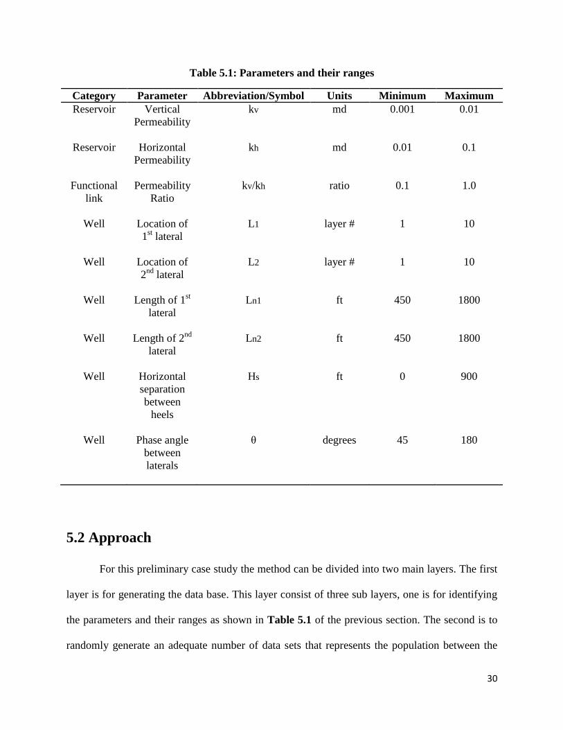
Table ‎5.1: Parameters and their ranges

Category Parameter Abbreviation/Symbol Units Minimum Maximum

Reservoir Vertical

Permeability

kv md 0.001 0.01

Reservoir Horizontal

Permeability

kh md 0.01 0.1

Functional

link

Permeability

Ratio

kv/kh ratio 0.1 1.0

Well

Location of

1st lateral

L1

layer #

1

10

Well

Location of

2nd

lateral

L2

layer #

1

10

Well

Length of 1st

lateral

Ln1

ft

450

1800

Well

Length of 2nd

lateral

Ln2

ft

450

1800

Well

Horizontal

separation

between

heels

Hs

ft

0

900

Well

Phase angle

between

laterals

θ

degrees

45

180

5.2 Approach

For this preliminary case study the method can be divided into two main layers. The first

layer is for generating the data base. This layer consist of three sub layers, one is for identifying

the parameters and their ranges as shown in Table 5.1 of the previous section. The second is to

randomly generate an adequate number of data sets that represents the population between the

31

parameters ranges. Then these data sets and other predefined reservoir properties and operating

conditions are combined to create many reservoir models which are fed to the numerical

simulator to generate the recovery profiles for each scenario. The established data base now is

the source for allocating the input and output parameters for developing the Forward and

Inverse-looking ANN solutions in the second layer. A simple flow chart summarizing the

process is illustrated in Figure 5.3. The details of the preliminary case study are presented in the

following sections. However before going any further what is meant by forward and inverse-

looking solutions? These two terms simply reflect the type of problem addressed and what the

known and unknowns are. For example, given the distance and the velocity of three different

transportation vehicles say, a car, an airplane and a train it is straight forward to solve for the

time it took each vehicle to travel the given distance, hence forward-looking. Whereas if given

the distance and travel time it is inferably to solve for the type of transportation used, whether it

was a car, an airplane or a train, hence inverse-looking.

32

Fig. ‎5.3: Preliminary Case Study Flow Chart.

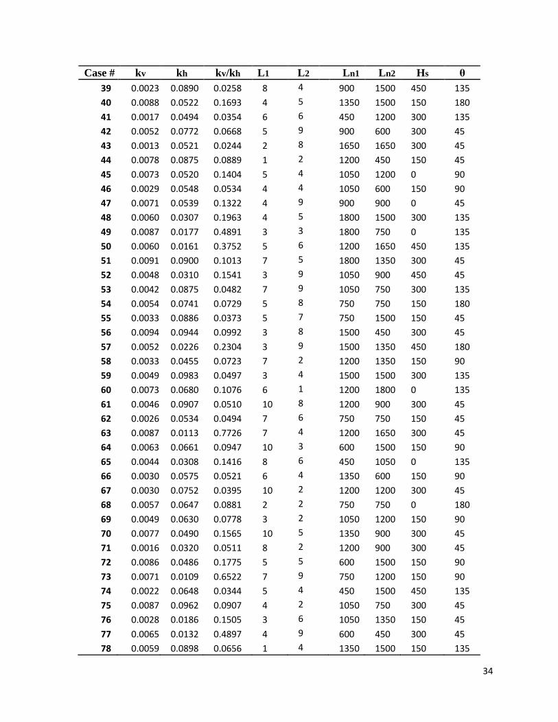
5.3 Data Base Generation

A pseudorandom code was used to generate 100 cases for different combinations of

reservoir properties and well parameters between the minimum and maximum values mentioned

in Table 5.1 as shown in Table 5.2. At this stage the remaining reservoir properties and

operating conditions were set constant. These constant parameters presented in Table 5.3 along

with the contents of Table 5.2 were combined to build the 100 scenarios introduced to the

numerical simulator. After running these models by the simulator the cumulative recovery

factors at 18 different time steps over a span of ~50 years were collected. With this process we

have concluded the data base required for developing the ANNs.

Develop The Artificial Neural Network Forward-Looking ANN

•Input Layer

•Output Layer

Inverse-Looking ANN

•Input Layer

•Output Layer

Generate Data Base

Identify Variables & Populate Data Between

Ranges Construct Data Sets

Feed Data Sets to Numerical Simulator &

Collect Results

33

Table ‎5.2: Pseudorandom Parameters

Case # kv kh kv/kh L1 L2 Ln1 Ln2 Hs θ

1

2

3

4

5

6

7

8

9

10

11

12

13

14

15

16

17

18

19

20

21

22

23

24

25

26

27

28

29

30

31

32

33

34

35

36

37

38

0.0084

0.0027

0.0021

0.0084

0.0067

0.0011

0.0091

0.0056

0.0059

0.0065

0.0078

0.0087

0.0044

0.0018

0.0076

0.0040

0.0086

0.0043

0.0085

0.0026

0.0022

0.0089

0.0014

0.0072

0.0076

0.0049

0.0044

0.0098

0.0046

0.0050

0.0024

0.0039

0.0038

0.0091

0.0032

0.0038

0.0047

0.0074

0.0870

0.0704

0.0571

0.0369

0.0734

0.0443

0.0611

0.0899

0.0859

0.0909

0.0945

0.0834

0.0101

0.0103

0.0179

0.0335

0.0121

0.0482

0.0407

0.0587

0.0934

0.0369

0.0404

0.0874

0.0406

0.0224

0.0557

0.0871

0.0446

0.0726

0.0665

0.0505

0.0526

0.0955

0.0175

0.0352

0.0502

0.0629

0.0960

0.0384

0.0370

0.2274

0.0919

0.0258

0.1484

0.0627

0.0687

0.0711

0.0830

0.1043

0.4392

0.1714

0.4255

0.1192

0.7101

0.0902

0.2077

0.0441

0.0232

0.2419

0.0345

0.0822

0.1871

0.2200

0.0793

0.1127

0.1030

0.0683

0.0363

0.0779

0.0727

0.0948

0.1840

0.1079

0.0932

0.1172

1

6

9

4

8

6

8

8

1

4

7

5

10

8

6

4

3

9

5

8

2

9

1

9

9

6

2

3

7

8

1

8

10

4

7

4

3

8

5

6

2

7

9

2

5

4

10

6

3

2

6

8

9

9

3

6

9

2

9

9

3

2

5

9

5

5

6

2

2

9

6

3

9

2

5

7

1050

1050

1650

1050

600

750

1350

1650

1800

750

1500

1200

1050

1200

1050

1350

1500

900

600

1500

1050

1500

750

600

1650

1650

1800

1650

450

1200

1800

1200

1650

600

1800

1650

1200

1050

1350

900

1800

600

750

1500

600

1200

1500

1500

600

1050

900

1050

1200

600

1650

1350

600

1200

1650

1500

1350

1050

750

1200

750

900

1650

1650

1500

1650

750

1200

1350

1650

1350

1050

150

150

450

300

150

0

300

300

0

0

450

150

0

0

0

450

150

300

150

0

450

150

150

300

150

150

300

450

300

150

150

150

0

450

300

150

300

0

180

90

45

90

180

180

90

90

45

45

135

45

45

90

135

45

135

45

45

90

135

45

45

180

90

45

180

180

45

45

135

135

45

45

90

90

90

45

34


39

40

41

42

43

44

45

46

47

48

49

50

51

52

53

54

55

56

57

58

59

60

61

62

63

64

65

66

67

68

69

70

71

72

73

74

75

76

77

78

0.0023

0.0088

0.0017

0.0052

0.0013

0.0078

0.0073

0.0029

0.0071

0.0060

0.0087

0.0060

0.0091

0.0048

0.0042

0.0054

0.0033

0.0094

0.0052

0.0033

0.0049

0.0073

0.0046

0.0026

0.0087

0.0063

0.0044

0.0030

0.0030

0.0057

0.0049

0.0077

0.0016

0.0086

0.0071

0.0022

0.0087

0.0028

0.0065

0.0059

0.0890

0.0522

0.0494

0.0772

0.0521

0.0875

0.0520

0.0548

0.0539

0.0307

0.0177

0.0161

0.0900

0.0310

0.0875

0.0741

0.0886

0.0944

0.0226

0.0455

0.0983

0.0680

0.0907

0.0534

0.0113

0.0661

0.0308

0.0575

0.0752

0.0647

0.0630

0.0490

0.0320

0.0486

0.0109

0.0648

0.0962

0.0186

0.0132

0.0898

0.0258

0.1693

0.0354

0.0668

0.0244

0.0889

0.1404

0.0534

0.1322

0.1963

0.4891

0.3752

0.1013

0.1541

0.0482

0.0729

0.0373

0.0992

0.2304

0.0723

0.0497

0.1076

0.0510

0.0494

0.7726

0.0947

0.1416

0.0521

0.0395

0.0881

0.0778

0.1565

0.0511

0.1775

0.6522

0.0344

0.0907

0.1505

0.4897

0.0656

8

4

6

5

2

1

5

4

4

4

3

5

7

3

7

5

5

3

3

7

3

6

10

7

7

10

8

6

10

2

3

10

8

5

7

5

4

3

4

1

4

5

6

9

8

2

4

4

9

5

3

6

5

9

9

8

7

8

9

2

4

1

8

6

4

3

6

4

2

2

2

5

2

5

9

4

2

6

9

4

900

1350

450

900

1650

1200

1050

1050

900

1800

1800

1200

1800

1050

1050

750

750

1500

1500

1200

1500

1200

1200

750

1200

600

450

1350

1200

750

1050

1350

1200

600

750

450

1050

1050

600

1350

1500

1500

1200

600

1650

450

1200

600

900

1500

750

1650

1350

900

750

750

1500

450

1350

1350

1500

1800

900

750

1650

1500

1050

600

1200

750

1200

900

900

1500

1200

1500

750

1350

450

1500

450

150

300

300

300

150

0

150

0

300

0

450

300

450

300

150

150

300

450

150

300

0

300

150

300

150

0

150

300

0

150

300

300

150

150

450

300

150

300

150

135

180

135

45

45

45

90

90

45

135

135

135

45

45

135

180

45

45

180

90

135

135

45

45

45

90

135

90

45

180

90

45

45

90

90

135

45

45

45

135

35


79

80

81

82

83

84

85

86

87

88

89

90

91

92

93

94

95

96

97

98

99

100

0.0025

0.0011

0.0079

0.0079

0.0048

0.0015

0.0063

0.0026

0.0076

0.0058

0.0033

0.0093

0.0078

0.0090

0.0016

0.0027

0.0076

0.0073

0.0080

0.0055

0.0048

0.0065

0.0322

0.0108

0.0833

0.0226

0.0892

0.0186

0.0417

0.0634

0.0627

0.0701

0.0683

0.0490

0.0226

0.0777

0.0318

0.0685

0.0872

0.0176

0.0975

0.0128

0.0852

0.0852

0.0764

0.0973

0.0953

0.3481

0.0537

0.0813

0.1503

0.0405

0.1206

0.0829

0.0480

0.1888

0.3465

0.1157

0.0510

0.0387

0.0876

0.4132

0.0820

0.4300

0.0567

0.0763

5

4

10

6

9

5

5

8

10

6

9

8

6

10

8

10

7

4

5

9

1

2

1

2

2

8

5

7

7

6

7

9

7

9

5

2

2

7

4

7

7

6

7

6

450

600

1800

1800

450

1050

1650

750

1650

1500

1350

450

900

1650

1350

900

1350

750

1200

1800

1650

900

1350

1800

600

1650

1200

1350

900

600

1650

600

900

1350

1800

1200

1800

750

1050

1350

600

1500

1050

1500

150

0

150

150

150

150

150

450

450

150

150

300

150

150

450

150

450

0

150

300

300

150

45

45

45

135

90

90

135

135

135

45

90

180

90

135

180

135

45

45

90

45

90

180

36

Table ‎5.3: Constant Reservoir Properties and Operating Parameters

Category Parameter Abbreviation/Symbol Units Value

Reservoir Drainage

Area DA Acres ~500

Reservoir

Total

Thickness

H ft 200

Reservoir Porosity Φ fraction 0.2

Reservoir

Temperature

TRES

°F

150

Reservoir

Initial

Pressure

Pi

psi

3500

Reservoir

Gas Density

ρg

lb/ft3

0.066

Operating

Condition

Minimum

Flowing

Bottom Hole

Pressure

Pwf

psi

500

Operating

Condition

Minimum

Gas Rate

Qg

Mscf/d

500

5.4 Forward-Looking ANN

This section will demonstrate the development of the Forward-looking ANN solution for

the preliminary case study. The purpose was to test the feasibility of developing a forecasting

expert system for reservoirs with a multilateral well that will serve as a proxy to the numerical

simulator and as a cross check mechanism in the absence of the numerical simulator later on in

this dissertation. The development gradually expands the base of the input layer, meaning that

the number of input parameters was gradually increased to include reservoir properties that were

previously set constant whereas the multilateral configurations were limited to a dual-lateral

37

only. Even though one of the main advantages of having an expert system is to know more with

less, however the end in mind here is to achieve a system with an acceptable generalization of

the problem that can distinguish the reservoir performance of many different combinations of

multilateral and reservoir properties.

5.4.1 Initial Forward-Looking ANN Solution

For the initial development the contents of Table 5.2 and the cumulative recovery

factors produced by the numerical simulator shown in Table 5.4 were the input and output data

respectively for constructing the ANN. Hence 100 cases with 9 parameters each, represented the

input layer, and a corresponding 100 cases with 18 cumulative recovery factors each, represented

the output layer. For building the network, it was elected to use the hyperbolic tangent sigmoid

‘tansig’ and the linear ‘purelin’ as the transfer functions, the conjugate gradient

backpropagation with Polak- Ribiére updates ‘traincgp’ as the training function, the gradient

descent with momentum weighted and bias learning function ‘learngdem’, and the mean

squared error with regularization performance function ‘msereg’ (MATLAB®, 2011).

38

Table ‎5.4: Cumulative Recovery Factors Produced by the Numerical Simulator

Time Step Case# 1 2 3 4 5 6 7 8 9 10

1 d 9.E-05 4.E-05 5.E-05 4.E-05 4.E-05 2.E-05 6.E-05 9.E-05 9.E-05 7.E-05 90 d 0.005 0.002 0.003 0.003 0.003 0.002 0.004 0.006 0.005 0.004

180 d 0.010 0.004 0.006 0.005 0.005 0.003 0.008 0.010 0.009 0.008 270 d 0.014 0.006 0.008 0.007 0.007 0.004 0.011 0.015 0.012 0.012 1 yr 0.018 0.008 0.011 0.009 0.009 0.005 0.014 0.019 0.016 0.015 2 yr 0.033 0.015 0.020 0.017 0.017 0.010 0.025 0.036 0.029 0.028 3 yr 0.047 0.022 0.028 0.024 0.024 0.015 0.036 0.051 0.042 0.040 4 yr 0.061 0.029 0.036 0.031 0.031 0.019 0.046 0.066 0.053 0.051 5 yr 0.073 0.036 0.044 0.037 0.038 0.023 0.056 0.079 0.065 0.062 6 yr 0.086 0.042 0.051 0.043 0.045 0.027 0.065 0.092 0.075 0.072 7 yr 0.098 0.048 0.059 0.049 0.052 0.032 0.074 0.105 0.086 0.082

14 yr 0.172 0.089 0.104 0.088 0.096 0.059 0.131 0.184 0.152 0.147 21 yr 0.236 0.127 0.144 0.122 0.135 0.084 0.180 0.249 0.208 0.202 28 yr 0.291 0.162 0.180 0.153 0.172 0.108 0.224 0.305 0.258 0.251 35 yr 0.340 0.194 0.213 0.183 0.206 0.131 0.264 0.354 0.302 0.295 42 yr 0.383 0.224 0.243 0.210 0.237 0.153 0.300 0.397 0.341 0.334 49 yr 0.421 0.252 0.271 0.235 0.267 0.174 0.332 0.435 0.377 0.370 50 yr 0.424 0.255 0.273 0.238 0.269 0.176 0.335 0.438 0.380 0.373 *d = day, yr = year

Cont. Table 5.4

Time Step Case# 11 12 13 14 15 16 17 18 19 20

1 d 7.E-05 7.E-05 2.E-05 1.E-05 3.E-05 3.E-05 4.E-05 4.E-05 3.E-05 5.E-05 90 d 0.005 0.004 0.001 0.001 0.002 0.002 0.003 0.003 0.002 0.003


14 yr 0.165 0.140 0.032 0.032 0.065 0.058 0.076 0.086 0.058 0.106 21 yr 0.226 0.193 0.045 0.044 0.090 0.082 0.104 0.121 0.082 0.148 28 yr 0.279 0.240 0.056 0.056 0.112 0.105 0.129 0.152 0.105 0.187 35 yr 0.327 0.282 0.067 0.068 0.133 0.126 0.152 0.181 0.127 0.222 42 yr 0.368 0.320 0.077 0.079 0.153 0.146 0.174 0.209 0.147 0.255 49 yr 0.406 0.355 0.087 0.089 0.172 0.165 0.194 0.234 0.167 0.285 50 yr 0.409 0.358 0.088 0.090 0.174 0.167 0.196 0.237 0.169 0.288

39

Cont. Table 5.4

Time Step Case# 21 22 23 24 25 26 27 28 29 30

1 d 5.E-05 6.E-05 2.E-05 6.E-05 6.E-05 4.E-05 6.E-05 1.E-04 4.E-05 7.E-05 90 d 0.003 0.004 0.001 0.003 0.004 0.002 0.004 0.006 0.003 0.004


14 yr 0.118 0.106 0.050 0.126 0.113 0.074 0.122 0.204 0.085 0.137 21 yr 0.166 0.145 0.071 0.177 0.155 0.101 0.170 0.276 0.119 0.188 28 yr 0.209 0.180 0.092 0.222 0.193 0.126 0.213 0.336 0.149 0.233 35 yr 0.249 0.211 0.111 0.263 0.227 0.149 0.251 0.388 0.178 0.274 42 yr 0.285 0.240 0.130 0.301 0.259 0.171 0.287 0.433 0.204 0.310 49 yr 0.318 0.267 0.148 0.335 0.288 0.191 0.319 0.473 0.229 0.344 50 yr 0.321 0.269 0.149 0.338 0.290 0.193 0.322 0.477 0.231 0.347

Cont. Table 5.4

Time Step Case# 31 32 33 34 35 36 37 38 39 40

1 d 5.E-05 5.E-05 4.E-05 7.E-05 3.E-05 5.E-05 6.E-05 5.E-05 4.E-05 9.E-05 90 d 0.003 0.003 0.002 0.004 0.002 0.004 0.004 0.003 0.003 0.005


14 yr 0.112 0.113 0.086 0.130 0.076 0.113 0.121 0.108 0.110 0.167 21 yr 0.158 0.158 0.121 0.180 0.105 0.155 0.168 0.150 0.155 0.227 28 yr 0.199 0.199 0.153 0.224 0.131 0.193 0.209 0.189 0.197 0.279 35 yr 0.237 0.236 0.183 0.264 0.155 0.227 0.246 0.224 0.235 0.325 42 yr 0.271 0.270 0.211 0.301 0.177 0.259 0.281 0.257 0.269 0.366 49 yr 0.303 0.301 0.237 0.334 0.198 0.288 0.312 0.287 0.302 0.402 50 yr 0.306 0.304 0.240 0.337 0.200 0.291 0.315 0.290 0.305 0.406

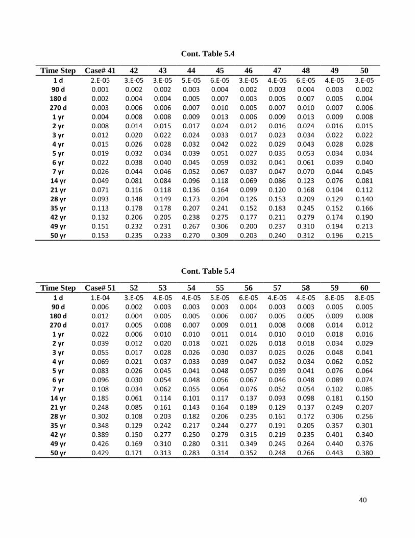
40

Cont. Table 5.4

Time Step Case# 41 42 43 44 45 46 47 48 49 50

1 d 2.E-05 3.E-05 3.E-05 5.E-05 6.E-05 3.E-05 4.E-05 6.E-05 4.E-05 3.E-05 90 d 0.001 0.002 0.002 0.003 0.004 0.002 0.003 0.004 0.003 0.002


14 yr 0.049 0.081 0.084 0.096 0.118 0.069 0.086 0.123 0.076 0.081 21 yr 0.071 0.116 0.118 0.136 0.164 0.099 0.120 0.168 0.104 0.112 28 yr 0.093 0.148 0.149 0.173 0.204 0.126 0.153 0.209 0.129 0.140 35 yr 0.113 0.178 0.178 0.207 0.241 0.152 0.183 0.245 0.152 0.166 42 yr 0.132 0.206 0.205 0.238 0.275 0.177 0.211 0.279 0.174 0.190 49 yr 0.151 0.232 0.231 0.267 0.306 0.200 0.237 0.310 0.194 0.213 50 yr 0.153 0.235 0.233 0.270 0.309 0.203 0.240 0.312 0.196 0.215

Cont. Table 5.4

Time Step Case# 51 52 53 54 55 56 57 58 59 60

1 d 1.E-04 3.E-05 4.E-05 4.E-05 5.E-05 6.E-05 4.E-05 4.E-05 8.E-05 8.E-05 90 d 0.006 0.002 0.003 0.003 0.003 0.004 0.003 0.003 0.005 0.005


14 yr 0.185 0.061 0.114 0.101 0.117 0.137 0.093 0.098 0.181 0.150 21 yr 0.248 0.085 0.161 0.143 0.164 0.189 0.129 0.137 0.249 0.207 28 yr 0.302 0.108 0.203 0.182 0.206 0.235 0.161 0.172 0.306 0.256 35 yr 0.348 0.129 0.242 0.217 0.244 0.277 0.191 0.205 0.357 0.301 42 yr 0.389 0.150 0.277 0.250 0.279 0.315 0.219 0.235 0.401 0.340 49 yr 0.426 0.169 0.310 0.280 0.311 0.349 0.245 0.264 0.440 0.376 50 yr 0.429 0.171 0.313 0.283 0.314 0.352 0.248 0.266 0.443 0.380

41

Cont. Table 5.4

Time Step Case# 61 62 63 64 65 66 67 68 69 70

1 d 5.E-05 2.E-05 4.E-05 6.E-05 2.E-05 4.E-05 4.E-05 4.E-05 6.E-05 5.E-05 90 d 0.003 0.001 0.003 0.004 0.001 0.002 0.003 0.002 0.003 0.003


14 yr 0.107 0.057 0.064 0.121 0.049 0.088 0.099 0.080 0.115 0.094 21 yr 0.150 0.081 0.085 0.168 0.070 0.125 0.139 0.113 0.161 0.131 28 yr 0.189 0.105 0.104 0.210 0.090 0.159 0.176 0.145 0.202 0.164 35 yr 0.225 0.127 0.121 0.248 0.109 0.190 0.209 0.174 0.239 0.195 42 yr 0.258 0.148 0.137 0.283 0.127 0.219 0.241 0.202 0.273 0.224 49 yr 0.289 0.169 0.152 0.314 0.145 0.246 0.270 0.228 0.305 0.251 50 yr 0.291 0.171 0.153 0.317 0.146 0.249 0.272 0.230 0.308 0.253

Cont. Table 5.4

Time Step Case# 71 72 73 74 75 76 77 78 79 80

1 d 2.E-05 6.E-05 3.E-05 3.E-05 6.E-05 2.E-05 1.E-05 8.E-05 2.E-05 1.E-05 90 d 0.001 0.004 0.002 0.002 0.004 0.002 0.001 0.005 0.001 0.001


14 yr 0.048 0.116 0.048 0.076 0.123 0.050 0.025 0.161 0.045 0.027 21 yr 0.069 0.159 0.065 0.108 0.171 0.070 0.035 0.222 0.064 0.038 28 yr 0.088 0.199 0.081 0.138 0.214 0.088 0.045 0.276 0.082 0.049 35 yr 0.107 0.234 0.096 0.167 0.254 0.105 0.054 0.323 0.100 0.059 42 yr 0.125 0.267 0.110 0.194 0.290 0.122 0.064 0.365 0.117 0.069 49 yr 0.142 0.297 0.124 0.219 0.323 0.137 0.072 0.403 0.133 0.078 50 yr 0.143 0.300 0.125 0.221 0.326 0.139 0.073 0.406 0.134 0.079

42

Cont. Table 5.4

Time Step Case# 81 82 83 84 85 86 87 88 89 90

1 d 6.E-05 6.E-05 5.E-05 2.E-05 5.E-05 2.E-05 9.E-05 5.E-05 5.E-05 5.E-05 90 d 0.004 0.004 0.003 0.001 0.003 0.001 0.005 0.003 0.003 0.003


14 yr 0.128 0.118 0.113 0.047 0.114 0.063 0.173 0.106 0.107 0.109 21 yr 0.178 0.160 0.159 0.067 0.157 0.091 0.236 0.148 0.150 0.151 28 yr 0.223 0.197 0.200 0.085 0.196 0.118 0.290 0.187 0.189 0.190 35 yr 0.263 0.231 0.238 0.103 0.231 0.143 0.337 0.222 0.225 0.225 42 yr 0.299 0.262 0.273 0.119 0.264 0.167 0.379 0.255 0.258 0.258 49 yr 0.333 0.291 0.305 0.135 0.294 0.189 0.416 0.285 0.289 0.288 50 yr 0.336 0.293 0.308 0.137 0.297 0.191 0.420 0.288 0.291 0.291

Cont. Table 5.4

Time Step Case# 91 92 93 94 95 96 97 98 99 100

1 d 5.E-05 9.E-05 3.E-05 3.E-05 7.E-05 3.E-05 7.E-05 3.E-05 8.E-05 8.E-05 90 d 0.003 0.005 0.002 0.002 0.004 0.002 0.004 0.002 0.004 0.005


14 yr 0.099 0.172 0.079 0.071 0.142 0.060 0.149 0.065 0.151 0.165 21 yr 0.133 0.236 0.111 0.102 0.194 0.081 0.207 0.087 0.208 0.227 28 yr 0.164 0.290 0.141 0.131 0.241 0.102 0.257 0.107 0.258 0.280 35 yr 0.192 0.339 0.170 0.159 0.282 0.120 0.302 0.125 0.302 0.328 42 yr 0.218 0.381 0.196 0.184 0.320 0.138 0.342 0.142 0.342 0.370 49 yr 0.243 0.419 0.221 0.209 0.354 0.155 0.378 0.158 0.378 0.407 50 yr 0.245 0.422 0.224 0.211 0.357 0.157 0.381 0.160 0.381 0.411

43

A network with an input layer of 9 neurons, an output layer of 18 neurons and

with a single hidden layer was set up. To determine the number of neurons contained by the

hidden layer that will yield the minimum error, a do loop from 2 to 100 neurons were tested and

stored the results for each loop. At the end of training each ANN set up the error between the

target or desired output and the predicted output for each network was calculated and the

network with the minimum error was selected. One hidden layer with 27 neurons resulted in the

lowest average error of 4.44% calculated using equation (5.1) where (RF) stands for recovery

factors, which is within acceptable limits for this case study. The accepted ANN architecture is

shown in Figure 5.4 and the corresponding regression plots are presented in Figure 5.5. When

executing this specific architecture it takes less than 5 seconds to obtain the corresponding

recovery factors of 100 combinations of reservoir properties and well configurations, whereas it

took around a couple of hours, using the interface code, to run the similar scenarios using the

numerical reservoir simulator and it could take a couple of days if run manually.

∑| |

( )

The overall process continuously divided the data sets randomly so that 70% of

the data set is allocated for training, 19% for validation and 11% for testing. The average

percentage error being tracked throughout this dissertation is of the testing data set since they are

not introduced to the network during the training and validation phase. Figure 5.6 demonstrates

cases 39 and 63 the best and the worst match respectively between the simulator and the ANN

recovery profiles predictions. The other 9 scenarios illustrated in Figure 5.7 show an overall

excellent match.

44

Fig. ‎5.4: ANN Architecture for the Initial Forward-Looking solution.

45

Fig. ‎5.5: Regression Plots for the Forward-Looking ANN solution of Fig. 5.4.

46

Fig. ‎5.6: Recovery Profile Predictions, ANN vs. Simulator, (best & worst match).

47

Fig. ‎5.7: The Remaining Comparison Plots for the Test set.

5.4.2 Expanded Forward-Looking ANN Solution

The expanded Forward-looking ANN featured a total of 17 input parameters

representing 8 reservoir properties, 6 well design parameters and 3 functional links as illustrated

in Table 5.5 and the objective remains the same, i.e. predicting the recovery profile at 18

different time steps. As mentioned previously the expansion to this point was done gradually by

moving parameters from the constant list of Table 5.3 to the variables introduced to the input

layer of the ANN. At this stage the pool of data has increased to a total of 1656 data sets.

Towards achieving a successful network 23 ANNs were tested against the simulator forecasts of

26 new data sets by varying the transfer, training and learning functions also by varying the

number of hidden layers and the number of neurons contained in each layer. The successful

ANN, network 18, consisted of two hidden layers, 22 and 29 neurons respectively. The log-

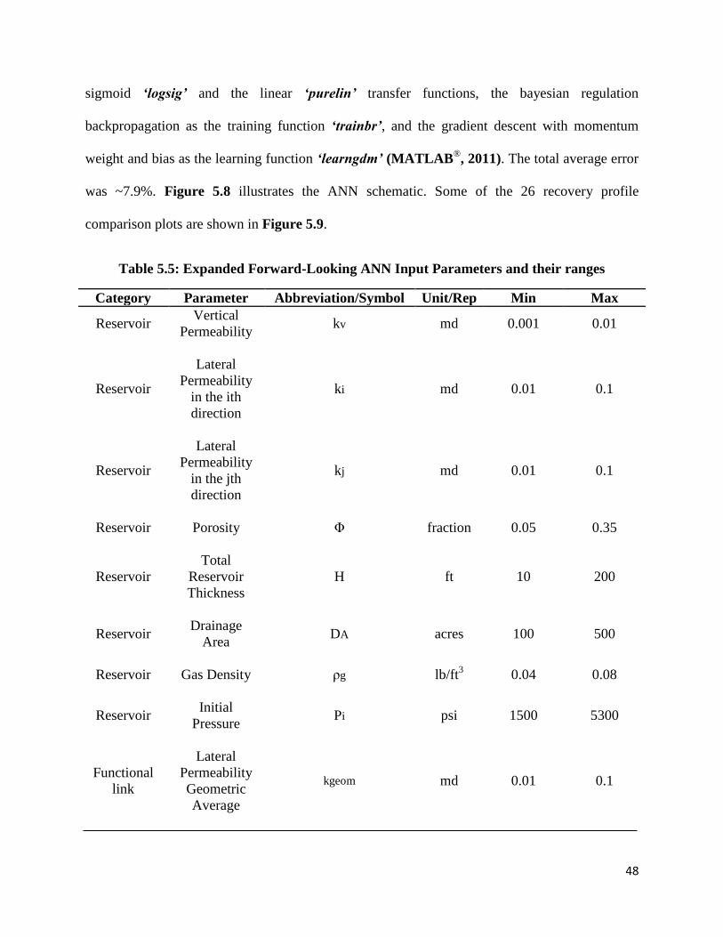
48

sigmoid ‘logsig’ and the linear ‘purelin’ transfer functions, the bayesian regulation

backpropagation as the training function ‘trainbr’, and the gradient descent with momentum

weight and bias as the learning function ‘learngdm’ (MATLAB®, 2011). The total average error

was ~7.9%. Figure 5.8 illustrates the ANN schematic. Some of the 26 recovery profile

comparison plots are shown in Figure 5.9.

Table ‎5.5: Expanded Forward-Looking ANN Input Parameters and their ranges

Category Parameter Abbreviation/Symbol Unit/Rep Min Max

Reservoir Vertical

Permeability kv md 0.001 0.01

Reservoir

Lateral

Permeability

in the ith

direction

ki md 0.01 0.1

Reservoir

Lateral

Permeability

in the jth

direction

kj md 0.01 0.1

Reservoir Porosity Φ fraction 0.05 0.35

Reservoir

Total

Reservoir

Thickness

H ft 10 200

Reservoir Drainage

Area DA acres 100 500

Reservoir Gas Density ρg lb/ft3 0.04 0.08

Reservoir Initial

Pressure Pi psi 1500 5300

Functional

link

Lateral

Permeability

Geometric

Average

kgeom md 0.01 0.1

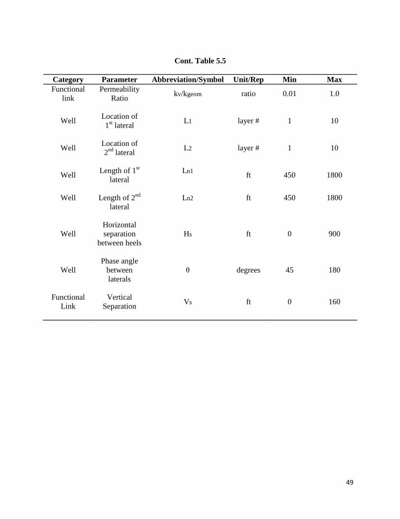
49

Cont. Table 5.5


Functional

link

Permeability

Ratio kv/kgeom ratio 0.01 1.0

Well Location of

1st lateral

L1 layer # 1 10

Well

Location of

2nd

lateral

L2

layer #

1

10

Well

Length of 1st

lateral

Ln1

ft

450

1800

Well

Length of 2nd

lateral

Ln2 ft 450

1800

Well

Horizontal

separation

between heels

Hs

ft

0

900

Well

Phase angle

between

laterals

θ

degrees

45

180

Functional

Link

Vertical

Separation Vs ft 0 160

50

Fig. ‎5.8: Expanded Forward-Looking Network #18 Architecture.

51

Fig. ‎5.9: Comparison Plots of the Recovery Profile Predictions (ANN vs. Simulator).

5.5 Inverse-Looking ANN

This section will demonstrate the development of the Inverse-looking ANN solution for

the preliminary case study. The purpose was to test the feasibility of developing an expert system

capable of recommending and suggesting the multi-lateral well architecture for a given set of

reservoir properties and a targeted recovery profile. Therefore, the objective here was somewhat

reversed from the forward-looking solution, hence the name, here the reservoir properties along

with the cumulative recovery factors at 18 different time steps were the inputs to the network to

52

solve for the dual-lateral well design parameters. Similar to the forward-looking solution, the

development gradually expands the base of the input layer, meaning that the number of input

parameters was gradually increased to include reservoir properties that were previously set

constant along with the corresponding cumulative recovery factors determined at 18 different

time steps.

5.5.1 Initial Inverse-Looking ANN Solution

Similar to the initial development of the forward-looking solution, the contents of

Tables 5.2 and 5.4 were used for extracting the input and output parameters for the network

however with a different order. In this case the reservoir properties, i.e. the normal and lateral

permeability and their ratios, combined with the corresponding cumulative recovery factors

produced by the numerical simulator at 18 different time steps were the input parameters to the

network with 21 neurons. Whereas the dual-lateral design parameters were the desired targets or

output layer of the network with 6 neurons.

Many ANN scenarios were explored by varying the number of hidden layers,

number of neurons per hidden layer, and the choice of transfer, training, and learning functions

until the minimum error criteria was achieved. The ANN model consisted of 21 input neurons,

two hidden layers with 45 and 26 neurons respectively, and 6 output neurons as illustrated in

Figure 5.10. The log-sigmoid ‘logsig’ and linear ‘purelin’ transfer functions, the Bayesian

regulation backpropagation training function ‘trainbr’, and the hebb with decay weight learning

rule ‘learnhd’ were applied in this network (MATLAB®, 2011).

53

The average relative error between targets and network predictions was significantly small, only

~0.02%! which resulted in a correlation coefficient, R, equal to one as shown in Figure 5.11.

However it turned out to be unworkable as the analysis indicated later on in this chapter.

Fig. ‎5.10: ANN Architecture for the Initial Inverse-Looking solution.

54

Fig. ‎5.11: Regression Plots for the Initial Inverse-Looking ANN solution of Fig. 5.10.

The process of randomly selecting 70% of the data set for training, 19% for

validating and 11% for testing was also applied here as well. Figure 5.12 demonstrates two

parameters of the 11 tested cases which indicated perfect matches between targeted and

predicted by the ANN. The other parameters comparison plots are illustrated in Figure 5.13

which also show a perfect match.

55

Fig. ‎5.12: Comparison Plots of Two Parameters for all Test Cases (ANN vs. Target).

56

Fig. ‎5.13: The Remaining Parameters Comparison Plots for all Test Cases.

5.5.2 Expanded Inverse-Looking ANN Solution

The expanded Inverse-looking ANN featured a total of 27 input neurons

representing 7 reservoir properties, 18 cumulative recovery factors and 2 functional links with a

corresponding output layer consisted of 7 neurons representing 6 well design parameters in

addition to the assigned drainage areas. Again heuristically developed a network with two hidden

layers containing 24 and 31 neurons respectively as shown in Figure 5.14. The log-sigmoid

‘logsig’ and the linear ‘purelin’ transfer functions, the bayesian regulation backpropagation as

the training function ‘trainbr’ and the hebb with decay weight learning rule ‘learnhd’ were

again used for this model (MATLAB®, 2011). The plots comparing the ANN predictions and the

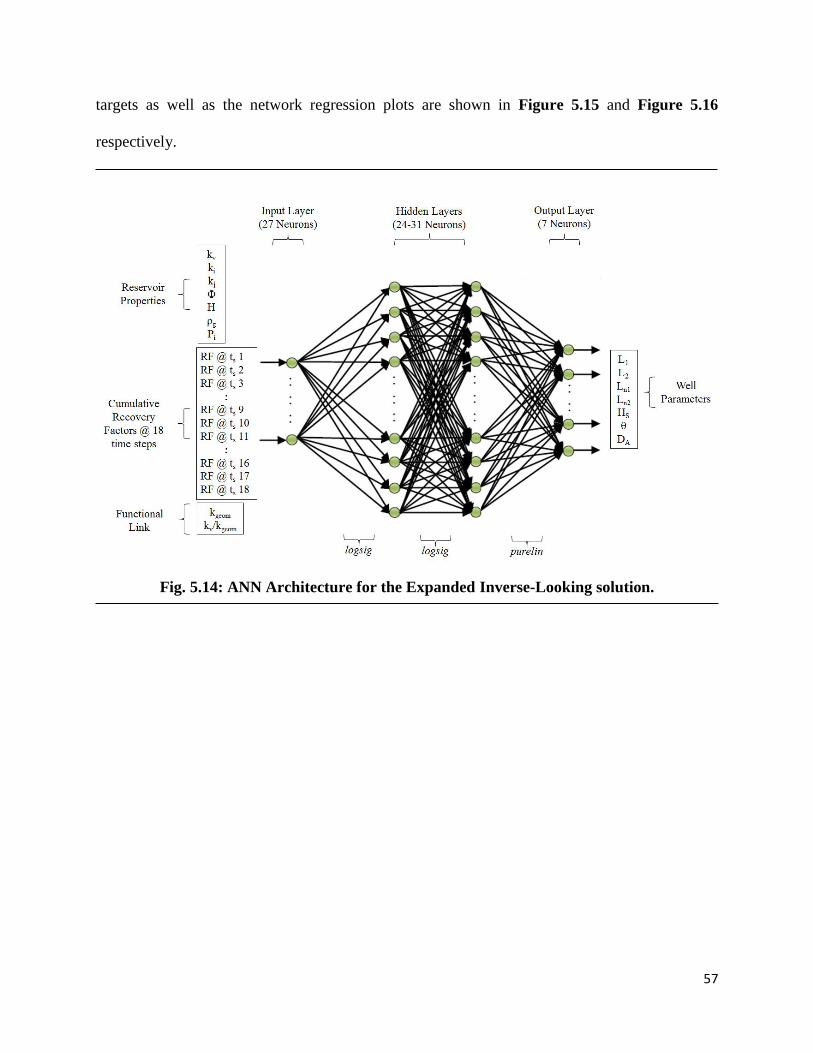
57

targets as well as the network regression plots are shown in Figure 5.15 and Figure 5.16

respectively.

Fig. ‎5.14: ANN Architecture for the Expanded Inverse-Looking solution.

58

Fig. ‎5.15: Parameters Comparison Plots of for all Test Cases (ANN vs. Target).

59

Fig. ‎5.16: Regression Plots for the Expanded Inverse-Looking ANN solution of Fig. 5.14.

5.5.2.1 Testing the Expanded Inverse-Looking ANN Solution

The almost perfect and too good to be true match between ANN predictions and

targets obtained by the initial and expanded Inverse-looking ANN solutions triggered a flag and

called for additional examinations. Testing the expanded network will suffice since it is supposed

to supersede all previous inverse-looking networks. Therefore, 18 new randomly generated, data

sets containing combinations of reservoir properties and dual-lateral configuration parameters

60

each within the limits mentioned in Table 5.5 were introduced to the numerical simulator. The

cumulative recovery factors at 18 different time steps corresponding to each reservoir and well

combination were obtained from the numerical simulator run. With this, the reference data base

to cross check the expanded inverse-looking predictions was complete. At this point, the

combination of the reservoir properties and recovery factors of the 18 new data sets were the

known parameters to solve for the unknown dual-lateral parameters and assigned drainage area

using the developed expanded inverse-looking network previously illustrated in Figure 5.14.

The outputs were compared with the targets, however indicated a network failure in

generalization capabilities as presented in Figure 5.17, hence the expanded inverse-looking

network had tumbled into the overfitting trap.

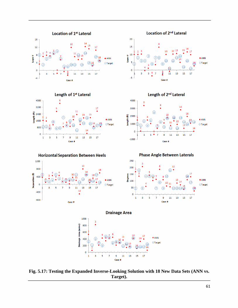
61

Fig. ‎5.17: Testing the Expanded Inverse-Looking Solution with 18 New Data Sets (ANN vs.

Target).

62

5.5.2.2 Overfitting

When networks fail to generalize from trends and tend to memorize training data

then the possibility of overfitting exists. It occurs when focus is on achieving a very small error

on the training set, however the error is large when new data is introduced to the network. There

are a few methods for enhancing ANN generalization.

One method is to use a network with the right size to deliver a good match. If the

network is too large the higher the degree of complexity it generates and if it is too small the

weaker it is to produce an acceptable fit. However knowing in advance how large a network

should be for a particular problem is in itself a challenging task.

Another technique is known as early stopping which is the default method for

improving generalization. In summary the way it works, as the name indicates, is that the

network is triggered when to stop training. In more details, generally when a data set is provided

to a network it is divided into three subsets namely a training set, a validation set and a testing

set. The training set is used for measuring the gradient to reassign the network weights and

biases. During the training phase the error in the validation set is observed. Usually at the

beginning of training the error in the validation and the training sets decreases, conversely when

the network starts to memorize the data hence overfits the data, the validation error increases.

Therefore, when the validation error continually increases for a predefined number of iterations

the network is triggered to terminate the training, then the weights and biases observed when the

validation error was at minimum are resumed (MATLAB®, 2011).

63

5.5.3 Modified Inverse-Looking ANN Solution

Taking into account the experience gained from the expanded Inverse-looking

ANN and how to overcome the memorization and overfitting problems, a modified inverse-

looking solution was developed. In the process a larger data set containing 1656 cases was used

in training, validating and testing 35 neural networks. Those networks were varied in size,

structure and functions. They had different number of hidden layers, different number of neurons

and different combinations of transfer, training and learning functions. In the logical and

physical sense all of the 35 networks, when tested with 26 new randomly generated data sets, had

an improved prediction and generalization capability over the expanded inverse-looking solution,

i.e. there were no predictions out of the previously defined ranges. Supporting this observation

are the results obtained by three neural networks as shown in Figure 5.18. However the variation

between targets and ANN outputs were still considered high.

64

Fig. ‎5.18: Results from Three Modified Inverse-Looking ANNs (ANN vs. Target).

65

An error analysis was performed on the 35 modified inverse-looking neural

networks to compare and understand their behavior. The average errors of the 26 testing cases

from each network for each parameter were compared as illustrated in Figure 5.19.

Fig. ‎5.19: Error Plots of Each Parameter/Network and the Total Average Error/Network.

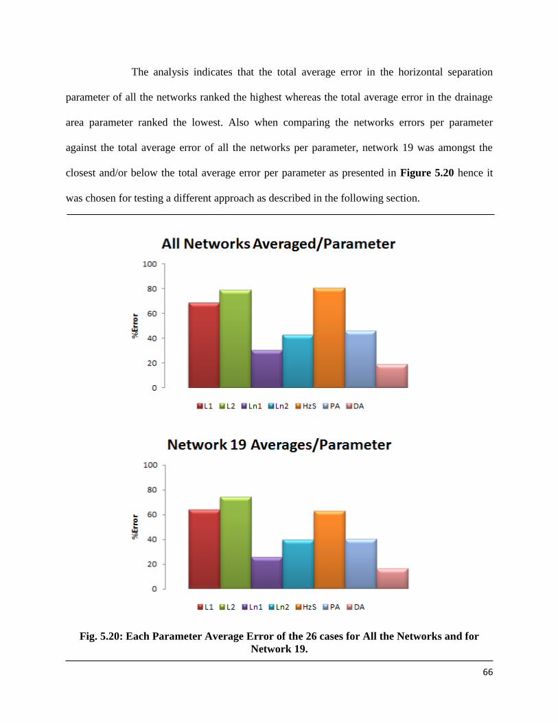
66

The analysis indicates that the total average error in the horizontal separation

parameter of all the networks ranked the highest whereas the total average error in the drainage

area parameter ranked the lowest. Also when comparing the networks errors per parameter

against the total average error of all the networks per parameter, network 19 was amongst the

closest and/or below the total average error per parameter as presented in Figure 5.20 hence it

was chosen for testing a different approach as described in the following section.

Fig. ‎5.20: Each Parameter Average Error of the 26 cases for All the Networks and for

Network 19.

67

5.5.4 Closed Loop Approach

Reflecting on the original purpose of developing an Inverse-Looking ANN

solution, is to predict the design parameters of a well and its assigned drainage area that will

produce a target recovery profile for a given set of reservoir properties. In the previous section,

the predicted parameters were compared with the targeted parameters only. However, given that

this is a pattern recognition problem, there is a possibility that the combination of the predicted

parameters will perform similar to the combination of the targeted parameters. In other words,

there may be more than one solution that could coexist, i.e. two different well configurations

could produce the same recovery profile for the same set of reservoir properties. This is a valid

assumption in field development. Therefore, the proposed closed loop approach is to generate the

performance of the predicted parameters combined by using the numerical simulator or the

Expanded Forward-Looking solution and compare it with the performance of the targeted

parameters combined. If the error between performances, i.e. target recovery profiles vs.

reproduced recovery profiles, is within tolerance then it is concluded that the inverse-looking

solution is successful and could be used for solving new data sets.

5.5.4.1 Crosschecking with the Numerical Simulator

The process generally is to crosscheck the modified inverse-looking networks one

by one by gathering the output parameters predicted by the network combine it with their

respective reservoir properties from the input set. Then use the numerical simulator to produce

their corresponding recovery profiles. Compare the simulator recovery profiles to the recovery

profiles located in the input set of the network and calculate the error. If the error is within

acceptable limits then the network is accepted otherwise it is rejected and a new inverse-looking

68

ANN is evaluated. Figure 5.21 summarizes the described process. For additional confirmation of

good generalization 100 new random combinations of reservoir properties and dual-lateral

parameters were generated, run by the numerical simulator and obtained their respective

recovery profiles. This establishes a new data base that was not introduced during the

development of the modified inverse-looking networks to use as targets and cross-referencing.

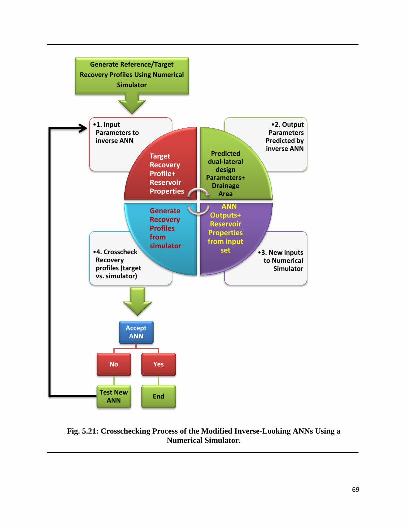
69

•3. New inputs to Numerical

Simulator

•4. Crosscheck Recovery profiles (target vs. simulator)

•2. Output Parameters

Predicted by inverse ANN

•1. Input Parameters to inverse ANN

Target Recovery Profile+ Reservoir Properties

Predicted dual-lateral

design Parameters+

Drainage Area

ANN Outputs+ Reservoir Properties from input

set

Generate Recovery Profiles from simulator

Accept ANN

No

Test New ANN

Yes

End

Fig. ‎5.21: Crosschecking Process of the Modified Inverse-Looking ANNs Using a

Numerical Simulator.

Generate Reference/Target

Recovery Profiles Using Numerical

Simulator

70

As hinted in the previous error analysis section, the crosschecking process

confirmed the success of network 19. An overall average error of ~12.2% was observed when

comparing the 100 recovery profiles generated by the numerical simulator using the dual-lateral

configurations and assigned drainage areas predicted by network 19 as new inputs and the

reference/target recovery profiles used as inputs to network 19. The modified inverse-looking

network 19 still had 27 input parameters and 7 outputs; it consists of two hidden layers with 15

and 22 neurons respectively as illustrated in Figure 5.22. The transfer functions are ‘logsig’ and

‘purelin’, the training function is ‘trainbr’ and ‘learngdm’ is the gradient descent with

momentum weight and bias learning function (MATLAB®, 2011).

Fig. ‎5.22: Modified Inverse-Looking Network #19 Architecture.

71

5.5.4.2 Crosschecking with the Expanded Forward-Looking ANN Solution

The process is almost the same as the previous one except for the use of the

numerical simulator is replaced by the successful expanded forward-looking network #18. The

reason for using the forward-looking solution is in case the tool or source used for generating the

reference or target recovery profiles in the first place is not available or allowed access to by the

client. Also this way the robustness of both the forward and inverse looking networks will be put

to the test. Figure 5.23 highlights the process and changes made.

72

•3. New inputs to Forward

ANN

•4. Crosscheck Recovery profiles (target vs. Fwd_ANN)


Predicted by inverse ANN

•1. Input Parameters to inverse ANN


Predicted dual-lateral

design Parameters+

Drainage Area

ANN Outputs+ Reservoir Properties from input

set

Generate Recovery Profiles from Forward_ ANN

Accept ANN

No

Test New ANN

Yes

End

Fig. ‎5.23: Crosschecking Process of the Modified Inverse-Looking ANNs Using the

Expanded Forward-Looking ANN Solution Network #18.

Provided Reference/Target

Recovery Profiles by the Client

73

Again, the modified inverse-looking network #19 was chosen for the test since it

was successful when crosschecked with the simulator. The predicted dual-lateral configuration

parameters and the assigned drainage area by the inverse network #19 were added to the input set

of the forward network #18 to predict the recovery profiles. Then both recovery profile sets from

the target and the forward ANN were compared.

To summarize, 9 cases from the inverse network #19 results were cross-examined

once using the numerical simulator and again with the forward network #18 applying the closed

loop approach, described earlier. Figure 5.24 illustrates the differences between the inverse

network #19 predictions, which are the dual-lateral configuration parameters and the drainage

areas, and the targeted parameters. It shows an overall average error of ~55.5% which is too

high. However when applying the combination of parameters predicted by the inverse network

#19 once to the simulator and once again to the forward network #18 to regenerate the recovery

profiles from both tools, very good matches were achieved. An overall average error for the total

100 cases of ~13.5% was observed when using the forward network #18 and ~12.2% when using

the simulator as mentioned previously, in addition the error between both crosschecking methods

was evaluated at ~5.2% as displayed in Figure 5.25, which demonstrate a very good agreement

between the forward network #18 and the simulator when having the similar inputs. The

recovery profile comparison plots of the same 9 cases presented earlier are shown in Figure

5.26. For each case there are three curves displayed, one illustrating the originally provided

recovery profiles needed to be achieved, hence called ‘Target’, the other is the recovery profile

obtained by using the numerical simulator where the dual-lateral parameters and assigned

drainage areas are those predicted by the inverse network #19, therefore named ‘Simulator’, and

the red dots represent the recovery profile obtained by using the forward network #18 by

74

assigning the same parameters predicted by the inverse network #19 to the input set and it’s

termed ‘Forward_ANN’.

Fig. ‎5.24: Parameters Predicted by the Inverse-Looking Network #19 for 9 Cases and

Compared With Targets.

75

Fig. ‎5.25: The Overall Average Error between Both Crosschecking Methods In Addition

To the Error between Both Tools.

76

Fig. ‎5.26: Comparison Plots of the Recovery Profiles Predicted by Both Methods vs. the

Targets for 9 Cases.

77

5.6 Summary and Lessons Learned

In this section the forward-looking and inverse-looking ANNs for forecasting recovery

profiles and advising dual-lateral design parameters respectively were successfully developed.

Both networks were tested against new data sets. The forward-looking solution for predicting

cumulative recovery factors for a range of volumetric single-phase gas reservoirs completed with

dual-lateral wells was tested with two new sets of data, the first containing 26 scenarios and

resulted in an average error of ~7.9% and the other contained 100 cases and returned an average

error of ~5.2%. The inverse-looking solution for designing the dual-lateral well configuration

was also tested with new 100 cases and returned an error of ~12.2% when crosschecked with the

numerical simulator, and ~13.5% when crosschecked with the forward-looking solution. In the

process of achieving these goals many challenging and demanding tasks were realized and

overcome by learning and developing new techniques, approaches and programs. These were

instrumental factors towards the development of the multi-lateral well design advisory system

and the reservoir forecasting and evaluation expert systems for the expanded form of volumetric

single phase gas reservoirs and the multiphase reservoirs with bottom water drive systems cases

which are presented in the next chapter. They served as a foundation of established methods and

techniques that led to a smooth expansion and transition process. Some of these tasks and lessons

learned were:

1. The application of a pseudorandom command for generating and populating data for any

given number of cases.

2. The development of a code that loads the data sets positions the wells and assigns the

reservoir properties then interfaces with the numerical simulator to automatically execute

all the scenarios provided. This was a crucial time saver for generating the data bases.

78

3. Another code that extracts critical information from the numerical simulator outputs.

4. Encountered and overcome an overfitting and memorization problem by changing the

learning function, retraining, increasing the size of the data and emphasizing early

stopping.

5. A closed loop approach proved the robustness of the inverse-looking solution.

6. It was observed that the training function ‘trainbr’ and the learning function ‘learnhd’

decrease in efficiency and takes a long time to converge when the data set is large.

Therefore new training and learning functions were explored during the development of

the integrated expert systems.

79

Chapter 6 Developed Expert Systems for Volumetric Single

Phase Gas Reservoirs

This chapter explains the development and the application of a set of artificial neural

networks in the area of forecasting, reservoir evaluation and multi-lateral well design. These

methods are developed and implemented to volumetric single phase gas reservoirs (VSPGR)

however with a variety of rock and fluid properties spanning unconventional, very tight, to

conventional sands and with the flexibility of employing a multi-lateral well ranging from 2 to 5

laterals.

6.1 Forecast Expert System (FExS) Development for Volumetric

Single Phase Gas Reservoirs (VSPGR)

The objective of developing this system is to deliver an acceptable performance forecast

in terms of cumulative recovery factors at 18 different time steps over a period of 50 years for a

given set of reservoir properties and a given multi-lateral well configuration.

6.1.1 Definition of Parameters

The parameters of Table 5.5 were modified to include permeability ranges that

expanded to account for unconventional and much tighter sands, added more laterals and their

corresponding lengths and locations. Table 6.1 lists the entire reservoir, operating and well

parameters definitions, units and ranges.

80

Table ‎6.1: Reservoir, Well Design and Operating Parameters and Their Ranges


Reservoir Vertical

Permeability kv md 1.0e-05 1.0e-4

Reservoir

Lateral

Permeability in

the ith direction

ki md 1.0e-04 0.1

Reservoir

Lateral

Permeability in

the jth direction

kj md 1.0e-04 0.1


Reservoir Total Reservoir

Thickness H ft 10 200

Reservoir Drainage Area DA acres 100 500


Reservoir Initial Pressure Pi psi 1500 5300

Functional

link

Lateral

Permeability

Geometric

Average

kgeom md 1.0e-04 0.1

Functional

link

Permeability

Ratio kv/kgeom ratio 1.0e-04 1.0

Operating

Minimum

Flowing Bottom

Pressure

Pwf psi 500 500

Operating Minimum Daily

Gas Rate Qg Mscf/d 500 500

Well Total # of

Laterals ML

# of

laterals 2 5

Well Location of 1

st

lateral L1 layer # 1 10

81

Cont. Table 6.1


Well Location of 2

nd


Well Location of 3

rd


Well Location of 4

th


Well Location of 5

th


Well Length of 1

st

lateral Ln1 ft/cell # 200/3 1800/12

Well Length of 2

nd


Well Length of 3

rd


Well Length of 4

th


Well Length of 5

th


Well

Horizontal

separation

between heels

Hs ft/cell # 1.0e-08 200/3

Well Phase angle

between laterals θ degrees 45 180

82

6.1.2 ANN Developments with Different Data Representations

One thousand new data sets were generated using the pseudorandom code in order

to include the additional parameters and ranges. During training the network many different data

representations were explored to enhance the accuracy and the generalization of the network. For

example, due to the tightness of some of the generated reservoir scenarios because of very low

permeability, they could not produce beyond three years as a result of reaching the minimum rate

cut-off of 500 thousand standard cubic feet per day or the minimum flowing bottom hole

pressure of 500 psi or both. The scenarios that could not sustain production beyond 3 years were

causing significant confusion to the learning process while training the network hence resulting

in large errors. Systematic and heuristic approaches were simultaneously administered while

reaching a successful neural network tool. A set of neural networks with 3 predefined hidden

layers and transfer functions however in different order, except for the last one was always the

default linear transfer function ‘purelin’, and with different do loops that varies the number of

neurons in each hidden layer were setup. Then heuristically, different data representations were

submitted as inputs and targets to these networks until the ANN with the lowest error was

achieved. The successful ANN had a data set of 718 cases that sustain production beyond 3 years

performers, represented their respective cumulative recovery factors and permeabilities with the

log10 of their original values. The structured ANN returned a solution with an error of 21%, the

details of the network are shown in Figure 6.1. At this point it was sought to further evaluate its

generalization capabilities on a new randomly generated data set as described in the following

section.

83

Fig. ‎6.1: FExS Implemented to Volumetric Single Phase Gas Reservoirs (VSPGR).

6.1.3 Testing Forecast Expert System (FExS) Applied to Volumetric

Single Phase Gas Reservoirs (VSPGR)

New randomly generated data sets, 84 of them, were used to test and crosscheck

the robustness of the latest developed forecast ANN presented in Figure 6.1. These cases

consisting of reservoir properties and multi-lateral well design configurations were fed to the

numerical simulator to generate their corresponding cumulative recovery factors. These results

were then used as references or targets to be achieved by the forecast expert system. The

cumulative recovery factors predicted by the forecast expert system had an overall average

deviation from the numerical simulator predictions of ~20.3%. Further analysis of the results

indicated that the maximum error was ~76% and the minimum was ~5% in addition to ~60% of

84

the predictions, i.e. 50 out of the 84 data sets, had errors below average. Figure 6.2 illustrates the

frequency of the data within ranges of error.

Fig. ‎6.2: FExS Results and Their Respective Errors Implemented to VSPGR .

Figure 6.3 presents some of the cases comparing target recovery profiles

(generated by the numerical simulator) and the FExS profiles (generated by the forecast expert

system).

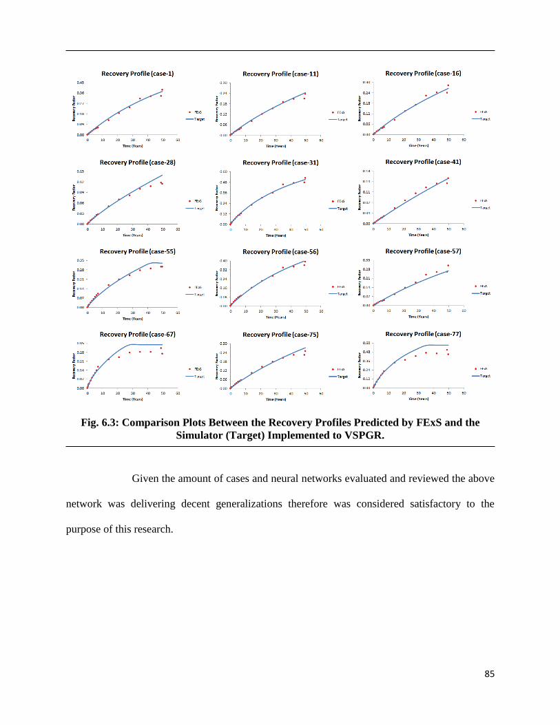
85

Fig. ‎6.3: Comparison Plots Between the Recovery Profiles Predicted by FExS and the

Simulator (Target) Implemented to VSPGR.

Given the amount of cases and neural networks evaluated and reviewed the above

network was delivering decent generalizations therefore was considered satisfactory to the

purpose of this research.

86

6.2 Multi-Lateral Well Design Advisory System (MLWDAS)

Development for Volumetric Single Phase Gas Reservoirs

The objective of developing this system is similar to the inverse-looking solution described

in chapter 5. That is to recommend the multi-lateral well design parameters that will produce a

target recovery profile for a given reservoir. However the system here is more complex in terms

of increase in number of outputs required where it was only 7 parameters in the inverse-looking

solution compared to 14 parameters for this system. In addition to the inclusion of much tighter

reservoir systems by expanding the range of permeability to cover very low values as displayed

in Table 6.1. Since this system is the reverse of the forecasting expert system they were

simultaneously developed by rearranging the input and output parameters for each system during

the rigorous scenarios explained in section 6.1.2. The ANN structure presented in Figure 6.4.

had an error of ~36%.

87

Fig. ‎6.4: MLWDAS Implemented to VSPGR.

6.2.1 Crosschecking Multi-Lateral Well Design Advisory System

(MLWDAS) using the Numerical Simulator

Although the ANN resulted in an overall average error of ~36% it is yet not

indicative enough of the robustness of the system, as proved during the inverse-looking

development in Chapter 5, since there could coexist more than one multi-lateral well design that

will have similar performances. Therefore the closed loop approach, described in section 5.5.4

also illustrated in Figure 6.5, was implemented for crosschecking.

88


Simulator

•4. Crosscheck Recovery profiles (target vs. simulator)


Predicted by MLWDAS

•1. Input Parameters to MLWDAS


Predicted Multi-lateral Well design

Parameters+ Drainage

Area

MLWDAS Outputs+ Reservoir Properties from input

set

Generate Recovery Profiles from simulator

Accept MLWDAS

No

Test New MLWDAS

Yes

End

Fig. ‎6.5: Crosschecking Process for MLWDAS Using the Numerical Simulator.

Provide Reference/Target

Recovery Profiles

89 *the code interfacing with the simulator missed two cases hence 82 instead of 84.

Eighty two* of the same 84 new data sets generated for testing FExS were used

for testing MLWDAS. Similarly the numerical simulator was applied to generate the

corresponding recovery profiles, referred to as target, for each of the 82 reservoirs and their

multi-laterals. Then the recovery profiles with their respective reservoir properties were inputs to

the MLWDAS. The MLWDAS generated its recommended multi-lateral well designs and

respective drainage areas for each of the 82 reservoirs. Even though these designs had an error of

~43% from the original 82 designs yet, as mentioned and proven, it is not an indicator of whether

these new designs will have similar performances or not. Therefore the MLWDAS

recommended well designs were combined with their respective reservoir properties and

assigned drainage areas and fed to the numerical simulator to generate their recovery profiles,

referred to as simulator. An overall average error of ~23.5% was measured when comparing both

recovery profiles, simulator vs. target, for the 82 cases. Furthermore, 47 cases had errors less

than the average error and only 13 cases had errors higher than 40% whereas the rest of the data

had errors in between as shown in Figure 6.6.

Fig. ‎6.6: MLWDAS Results and Their Respective Errors Implemented to VSGRs.

90


(MLWDAS) using Forecast Expert System (FExS)

Here the MLWDAS recommended well designs were combined with their

respective reservoir properties and assigned drainage areas and fed to the forecast expert system

(FExS) to predict their recovery profiles, referred to as FExS. Again this is a closed loop

approach as demonstrated in Figure 6.7. This process, as said, ‘hits two birds with one stone’

since while confirming that the MLWDAS recommended well designs perform as targeted, i.e.

FExS vs. Target, in the same time the FExS robustness will be examined and crosschecked with

the simulator results obtained from the previous crosschecking when using the numerical

simulator, i.e. Target vs. Simulator.

91

•3. New inputs to FES

•4. Crosscheck Recovery profiles (target vs. FES)


Predicted by MLWDAS

•1. Input Parameters to MLWDAS


Predicted Multi-lateral Well design

Parameters+ Drainage

Area

MLWDAS Outputs+ Reservoir Properties from input

set

Generate Recovery Profiles Using FES

Accept MLWDAS

No

Test New MLWDAS

Yes

End

Fig. ‎6.7: Crosschecking Process for MLWDAS Using FExS.

Provide Reference/Target

Recovery Profiles

92

FExS vs. Target

The average error was ~20.8% when comparing the recovery profiles predicted by FExS

using the MLWDAS recommended well designs with the original 84 data sets recovery profiles,

referred to as targets, which is considered a good generalization for most of the data. Figure 6.8

illustrates the cases distribution with respect to their ranges of error.

Fig. ‎6.8: FExS vs. Target 84 Cases Distribution with Respect to their Ranges of error

Implemented to VSPGR.

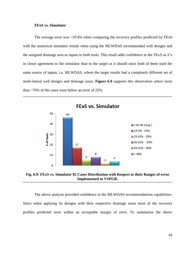
93

FExS vs. Simulator

The average error was ~19.4% when comparing the recovery profiles predicted by FExS

with the numerical simulator results when using the MLWDAS recommended well designs and

the assigned drainage area as inputs to both tools. This result adds confidence to the FExS as it’s

in closer agreement to the simulator than to the target as it should since both of them used the

same source of inputs, i.e. MLWDAS, where the target results had a completely different set of

multi-lateral well designs and drainage areas. Figure 6.9 supports this observation where more

than ~76% of the cases were below an error of 25%.

Fig. ‎6.9: FExS vs. Simulator 82 Cases Distribution with Respect to their Ranges of error


The above analysis provided confidence in the MLWDAS recommendations capabilities.

Since when applying its designs with their respective drainage areas most of the recovery

profiles predicted were within an acceptable margin of error. To summarize the above

94

crosschecking results and put them in perspective the overall average error for each process and

the recovery profiles comparison plots of some of the cases are illustrated in Figure 6.10.

95

Fig. ‎6.10: Recovery Profiles Predicted by Both Crosschecking Methods for MLWDAS


96

6.3 Reservoir Evaluation Expert System (REExS) Development for

Volumetric Single Phase Gas Reservoirs (VSPGR)

The realizations attained in the forecast expert system (FExS) and in the multi-lateral well

design advisory system (MLWDAS) led to the development of the reservoir evaluation expert

system (REExS). The general theme in the previous developments thus far has been solving for

one unknown. For applying the FExS, the multi-lateral design configurations and the reservoir

properties were the inputs to solve for or forecast the reservoir performance, hence FExS.

Likewise when using the MLWDAS, the reservoir performance and reservoir properties were

required knowledge for the MLWDAS to recommend well designs. Therefore, it naturally

follows the need for developing a system that will provide an assessment of the reservoir

properties, hence REExS. These three entities are intertwined where a change in one would

affect the other two. Figure 6.11 provides an illustration of the overall concept and the required

knowledge for using each system.

97

Performance

Design

Properties

Production

Performance

Well

Architecture

Reservoir

Properties

Production

Performance

Well

Architecture

Reservoir

Properties

Production

Performance

Well

Architecture

Reservoir

Properties

Fig. ‎6.11: General Theme of the Expert Systems Development Progression.

98

In the previous two developments, i.e. FExS and MLWDAS, it was, in concept, simply

switching between inputs and outputs. However, for practical reasons, this was not the case for

developing the reservoir evaluation expert system (REExS). Reasonably, evaluation of a

reservoir to obtain or reassess its properties would not be of much importance when it’s mature,

inversely a reservoir evaluation is of great value when done earlier in its production life.

Therefore, it couldn’t be a matter of reorganizing inputs and outputs. Instead of the long term

performances applied in the previous two developments a short term performance was required

for developing the REExS.

6.3.1 Testing Reservoir Evaluation Expert System (REExS)

Development for Volumetric Single Phase Gas Reservoirs (VSPGR)

To be able to develop a system that would provide an estimate of the reservoir

properties early in its development. It required an early indication of its performances. Therefore

the observed rate decline combined with their production periods were used for training the

networks. As the previous developments, over 500 new combinations of wells and reservoir

properties were randomly generated in addition to a new parameter to the ones listed in Table

6.1 and that is the production time which ranges from 1 – 60 months. The generated scenarios

combining production time, reservoir properties and multi-lateral well designs were run by the

numerical simulator to produce their matching rate declines at 18 different time steps which are

referred to as observed rate declines. Then the ANN was setup with the observed rate declines

and its corresponding multi-lateral well designs as inputs and the reservoir properties as outputs

or targets as illustrated in Figure 6.12.

99

Fig. ‎6.12: REExS Implemented to VSPGR.

After constructing and testing many ANNs the above network was thus far used

for predicting the reservoir properties. The network error was high when comparing target

reservoir properties to predicted ones. Figure 6.13 illustrates this by a sample of 10 cases

showing some of the parameters discrepancies.

100

Fig. ‎6.13: REExS Testing Results on 10 Cases Implemented to VSPGR..

101

However similar to what was observed during the development of the MLWDAS

where not all of the parameters could agree at once hence the conclusion of more than one

solution or design that will deliver the same performance for the same reservoir, which was

confirmed by the closed loop approach. Also the combination of the predicted parameters would

consequently result in a close match of the observed rate decline using the same well design.

Nonetheless, practically speaking, total ignorance of all of these reservoir properties is not the

case in reality. There must have been some hints or basic knowledge of some of these properties

that are relatively unpretentious to obtain while taking surveys and/or drilling wild cats

(exploration wells). In effect these properties would be used as controlling points for estimating

other properties that are arduous to gather otherwise. Hence this ANN will serve as a

scientifically engineered method for adjusting unknown or uncertain reservoir parameters until

an acceptable match of the observed rate decline is achieved.

To test the robustness of the system’s pattern recognition capabilities the concept

of the closed loop approach was implemented using the numerical simulator to crosscheck the

results obtained from REExS. In addition, in case of the unavailability of a numerical simulator

and to have the package integrating the expert systems function as a standalone product with a

360° approach, a Rate Decline Expert System (RDExS) was developed to allow flexibility to the

engineer to cross-examine the results obtained from REExS using RDExS. Therefore, before

testing the REExS, the next section will describe the development of the rate decline expert

system.

102

6.4. Rate Decline Expert System (RDExS) Development for


This system could be observed as a forward-looking solution similar in concept to the

FExS. As illustrated in Figure 6.11 FExS is a performance forecasting tool which requires the

knowledge of the reservoir properties and its multi-lateral well design. Similarly the rate decline

is another performance indicator however for the short term and displays rates instead of

cumulative recovery profiles. It is also the exact opposite of the reservoir evaluation expert

system. Therefore, the order of inputs and outputs were swabbed for developing the rate decline

ANN, where the reservoir properties, the production times and the multi-lateral design

parameters were used as inputs to the system and the rate decline data as the system targets or

outputs. Figure 6.14 illustrates the architecture of the developed rate decline ANN.

103

Fig. ‎6.14: RDExS Implemented to VSPGR.

6.4.1 Testing Rate Decline Expert System (RDExS) Applied to


The above network was tested with the same 48 scenarios used for testing the

REExS and compared with the numerical simulator results. The overall average error was ~30%

however more than ~71% of the scenarios, i.e. 34 cases, had an average error of only ~22%

whereas the remaining 14 cases had an average error of ~52% which indicates that just a few

cases had high errors which skewed the average error towards the high end. Figure 6.15

illustrates the cases distribution with respect to their error ranges. With this analysis it was safe

to utilize the RDExS as a crosschecking mechanism for REExS.

104

Fig. ‎6.15: RDExS vs. Simulator 48 Cases Distribution with Respect to Their Ranges of

error Implemented to VSPGR.

6.4.1.1 Crosschecking the REExS with the Numerical Simulator

As discussed earlier, though the REExS resulted in high discrepancies when

comparing reservoir properties predicted against targeted, it is yet not indicative enough of the

robustness of the system in terms of pattern recognition. Therefore the closed loop approach

illustrated in Figure 6.16 was implemented for crosschecking.

105


Simulator

•4. Crosscheck Rate profiles (observed vs. simulator)


Predicted by REExS

•1. Input Parameters to REExS

Observed Rate Decline+Well Design+Prod Time

Predicted Reservoir Properties

REExS Outputs+

Well Design+Prod

Time

Generate Rate Decline Profiles from Simulator

Accept REExS

No

Test New REExS

Yes

End

Fig. ‎6.16: Crosschecking Process for REExS Using the Numerical Simulator.

Provide Observed/Target

Rate Declines

106

The 48 new data sets generated for directly testing REExS & RDExS were used

again for indirect testing of REExS. The numerical simulator was applied to generate the

corresponding rate decline profiles, referred to as target or observed, for each of the 48 reservoirs

and their multi-laterals. Then the rate profiles with their respective multi-lateral well designs and

production times were inputs to the REExS. The REExS generated its reservoir properties

estimations for each of the 48 cases. Even though these properties were different from the

original set used in the numerical simulator to produce the target rate declines yet it is not an

indicator of whether these new properties would result in similar performances or not. Therefore

the REExS predicted reservoir properties combined with their respective well designs and

production periods were fed to the numerical simulator to generate their rate decline profiles,

referred to as simulator. An overall average error of ~34.6% was measured when comparing both

rate profiles, simulator vs. observed, for the 48 cases. The distribution of the cases with respect

to their average error ranges are shown in Figure 6.17. However it’s worth noting that 29 cases

had an average error of only ~20% whereas the remaining 19 cases had an average error of

~57%.

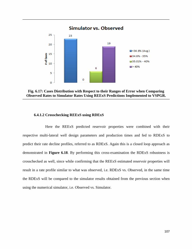
107

Fig. ‎6.17: Cases Distribution with Respect to their Ranges of Error when Comparing

Observed Rates to Simulator Rates Using REExS Predictions Implemented to VSPGR.

6.4.1.2 Crosschecking REExS using RDExS

Here the REExS predicted reservoir properties were combined with their

respective multi-lateral well design parameters and production times and fed to RDExS to

predict their rate decline profiles, referred to as RDExS. Again this is a closed loop approach as

demonstrated in Figure 6.18. By performing this cross-examination the RDExS robustness is

crosschecked as well, since while confirming that the REExS estimated reservoir properties will

result in a rate profile similar to what was observed, i.e. RDExS vs. Observed, in the same time

the RDExS will be compared to the simulator results obtained from the previous section when

using the numerical simulator, i.e. Observed vs. Simulator.

108

• 3. New inputs to

RDExS

•4. Crosscheck Rate profiles (observed vs. RDExS)


Predicted by REExS

•1. Input Parameters to REExS

Observed Rate Decline+Well Design+Prod Time

Predicted Reservoir Properties

REES Outputs+

Well Design+Prod

Time

Generate Rate Decline Profiles from RDExS

Accept REExS

No

Test New REExS

Yes

End

Fig. ‎6.18: Crosschecking Process for REExS Using RDExS.

Provide Observed/Target

Rate Declines

109

Similar to the previous process when crosschecking with the numerical simulator,

the so called observed rates and resepective well designs and production times of the 48 cases

were inputs to REExS. Which in turn provides an estimation of the, aught to be corresponding,

reservoir properties. Then to examine if this is true, these properties and the same set of well

designs and production times were fed this time to the RDExS instead of the numerical

simulator. The RDExS subsquently generated rate decline profiles for each of the 48 scenarios,

referred to as RDExS. Hence these RDExS rate profiles were compared to the observed rate

declines originally used to predict the reservoir properties. This resulted in an overall average

error of ~48.4% which was considered high, nevertheless the break down of the cases with

respect to their ranges of error indicated that 26 cases were below an average error of ~29%

whereas 22 cases had average errors above 55% as illustrated in Figure 6.19.

Fig. ‎6.19: Cases Distribution with Respect to their Ranges of Error when Comparing

Observed Rates to RDExS Rates Using REExS Predictions Implemented to VSPGR.

110

In general both crosschecking methods show a good generalization and trend

detection. The rate declines were broken into two groups. Group one, Figure 6.20, shows the

tendency of the rate declines generated by both approaches to match the observed rate declines

though the simulator rates were closer in most cases. The other group, Figure 6.21, highlights

the cases that display a good agreement between the numerical simulator predictions and the

RDExS rates. Eventhough these results mildly agree with the observed rates yet they add

confidence to the RDExS estimates since both tools, i.e. the simulator and the RDExS had the

same inputs from the same source, the REExS predictions.

111

Fig. ‎6.20: Rate Declines Predicted by Both Crosschecking Methods Using the REExS

Inputs Implemented to VSPGR.

112

Fig. ‎6.21: Rate Declines Predicted by Both Crosschecking Methods Using the REExS

Inputs.

113

Chapter 7 Developed Expert Systems for Multi-Phase

Reservoirs with Bottom Water Drive

This chapter highlights the developed expert systems implemented to Multi-Phase

Reservoirs with Bottom Water Drive (MPRBWD) with a variety of rock and fluid properties

spanning slightly tight sands to conventional sands and with the flexibility of employing a multi-

lateral well ranging from 2 to 5 laterals. Five distinct artificial neural networks are developed

here, the Forecast Expert System (FExS) which predicts the cumulative % recoveries, however

with added features that allow for more customization and flexibility such as the period desired

to run the forecast for, and the initial maximum oil rate desired to produce at. The Multi-Lateral

Well Design Advisory System (MLWDAS) also developed with the capability of specifying the

initial maximum oil rate and time for which the target performance is covering. The Reservoir

Evaluation Expert System (REExS) that partially characterizes the reservoir by predicting the

permeability values in the normal and both lateral directions, the porosity, the reservoir thickness

and the drainage area, however here with the inputs being the cumulative fluid production rather

than rate decline since the subject reservoirs are multi-phase with the primary hydrocarbon

production is oil in addition to the well configuration in place, other reservoir properties and the

production duration. The Cumulative Fluid Production Expert System, called CFPExS for short,

basically the inverse solution of REExS, to allow for a 360° approach in order to crosscheck the

REExS results in case of the absence or unavailability of a numerical simulator, which can be

used to reproduce the observed cumulative fluid production using the combination of properties

predicted by REExS and the existing well design. The fifth one is another forecasting tool

however with the capability of predicting the cumulative oil and gas productions, for how long is

114

the plateau and when is the abandonment times for a given initial maximum oil rate and a set of

reservoir and well design parameters, which as termed Cumulative-Abandonment-Plateau-Time-

Expert-System, and referred to as CAPTExS for short.

7.1 Definition of Parameters

The parameters of Table 6.1 is modified to include the added parameters and modified

ranges for existing properties normally common for multi-phase reservoirs with bottom water

drive. Table 7.1 lists the entire reservoir, operating and well parameters definitions, units and

ranges. A total of 2000 new cases are generated to populate the data base used for developing the

expert systems described in this chapter.

115

Table ‎7.1: Reservoir, Well Design and Operating Parameters and Their Ranges


Reservoir Vertical

Permeability kv md 0.1 50

Reservoir

Lateral

Permeability in

the ith direction

ki md 1.0 500

Reservoir

Lateral

Permeability in

the jth direction

kj md 1.0 500


Reservoir Total Reservoir

Thickness H ft 10 250

Reservoir Drainage Area DA acres 100 500


Reservoir Oil Density ρo lb/ft3 50 58

Reservoir Initial Pressure Pi psi 1500 5300

Reservoir Bubble Point

Pressure Pb psi 1500 5300

Reservoir

Depth to Top of

Reservoir from

Surface

DTOP ft 3000 10000

Operate

Maximum

Initial Daily Oil

Rate

Qo STB/D 2000 10000

Operate

Minimum

Flowing Bottom

Pressure

Pwf psi 14.7 14.7

Monitor Minimum Daily

Oil Rate Qo STB/D 50 50

116

Cont. Table 7.1


Monitor Maximum Gas

Oil Ratio GOR SCF/STB 4000 4000

Monitor Maximum

Water Cut wc % 99 99

Well Total # of

Laterals ML

# of

laterals 2 5

Well Location of 1

st


Well Location of 2

nd


Well Location of 3

rd


Well Location of 4

th


Well Location of 5

th


Well Length of 1

st


Well Length of 2

nd


Well Length of 3

rd


Well Length of 4

th


Well Length of 5

th


Well

Horizontal

separation

between heels

Hs ft/cell # 1.0e-08 200/3

Well Phase angle

between laterals θ degrees 45 180

117

7.2 Forecast Expert System (FExS) Development for Multi-Phase

Reservoirs with Bottom Water Drive (MPRBWD)

This system is similar in concept to the forecast system developed for implementation in

the Volumetric Single Phase Gas Reservoirs (VSPGR), described in section 6.1.2., however with

added parameters and features that help increase the accuracy and allows more flexibility for

customizing and testing different scenarios. In this set up six additional parameters are

introduced to the network input. The top depth of the reservoir from surface, the oil density, the

original oil in place, the bubble point pressure, the initial maximum oil rate and the period the

user wants to forecast for ranging from a year to 60 years. The time and initial oil rate added

features give the user the flexibility to examine variable performances for a unique combination

of reservoir properties and well design parameters. Whereas the top depth and original oil in

place help increase the accuracy of the network by increasing the uniqueness of each case.

Figure 7.1 illustrates the structured ANN for this system consisting of 27 inputs 5 hidden layers

with 70, 65, 60, 50 and 30 neurons respectively and 18 outputs. The objective of developing this

system is to deliver an acceptable performance forecast in terms of cumulative % recoveries at

18 different time steps covering the period provided by the user for a subject reservoir and its

well design parameters.

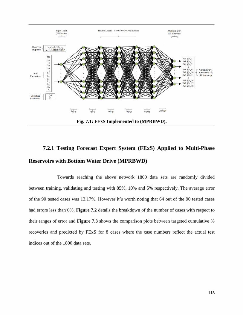
118

Fig. ‎7.1: FExS Implemented to (MPRBWD).

7.2.1 Testing Forecast Expert System (FExS) Applied to Multi-Phase

Reservoirs with Bottom Water Drive (MPRBWD)

Towards reaching the above network 1800 data sets are randomly divided

between training, validating and testing with 85%, 10% and 5% respectively. The average error

of the 90 tested cases was 13.17%. However it’s worth noting that 64 out of the 90 tested cases

had errors less than 6%. Figure 7.2 details the breakdown of the number of cases with respect to

their ranges of error and Figure 7.3 shows the comparison plots between targeted cumulative %

recoveries and predicted by FExS for 8 cases where the case numbers reflect the actual test

indices out of the 1800 data sets.

119

Fig. ‎7.2: FExS Results and Their Respective Errors Implemented to MPRBWD.

120

Fig. ‎7.3: Comparison Plots Between the Recovery Profiles Predicted by FExS and the

Simulator (Target) Implemented to MPRBWD.

121

7.3 Multi-Lateral Well Design Advisory System (MLWDAS)

Development for Multi-Phase Reservoirs with Bottom Water Drive

(MPRBWD)

Similar to its development in section 6.2 for the Volumetric Single Phase Gas Reservoirs

(VSPGR) where the multi-lateral well design parameters along with its assigned drainage area

are switched to the output layer and the target % recoveries are combined with the reservoir

properties and operating parameters at the input layer. From previous experience gained in

developments of this particular problem, the success criteria here is measured by comparing the

reservoir performance resulted by completing the target reservoir with the predicted well design

parameters to the target reservoir performance of the same reservoir provided as input to the

network. This is done by implementing one of the closed loop approach concepts outlined in

sections 6.2.1 and 6.2.2 and summarized in Figures 6.5 and 6.7 for using a numerical simulator

or the FExS, developed for MPRBWD in this case, respectively.

7.3.1 Multi-Lateral Well Design Advisory System (MLWDAS) ANN

Architecture

The same data set, 1800 cases, used for developing FExS in this chapter are

rearranged for training, validating and testing the ANN structures for developing the MLWDAS

used for MPRBWD. The successful network is shown in Figure 7.4. It consists of two hidden

layers with 40 and 35 neurons respectively, 31 input parameters grouped into sets of reservoir

properties, target cumulative percent recoveries at 18 time steps over a specified period of time,

and operating parameters. The output layer contains 14 neurons representing 13 multi-lateral

122

well design parameters and the proposed drainage area. The developed network returned an

overall absolute average error of 7 comparing between target and predicted well design

parameters, however as mentioned before, the key performance indicator here for the success of

the network is testing the performance of the predicted well design against the targeted

performance using one of the closed loop approaches.

Fig. ‎7.4: MLWDAS Implemented to MPRBWD.


(MLWDAS) with the Numerical Simulator

Eighty eight multi-lateral well design sets predicted by MLWDAS are tested

using the numerical simulator by combining them with their corresponding reservoir properties

and operating parameters to reproduce the cumulative recoveries and compare each to the target

123

cumulative recovery. The crosschecking resulted in an overall average error of ~8.38% where 59

cases had an overall average error of less than 4.2% as displayed in Figure 7.5. Eight cases are

shown in Figure 7.6 comparing target versus simulator cumulative recoveries.

Fig. 7.5: Target vs. Simulator of 88 Cases According to their Ranges of Error Implemented

to MPRBWD.

124

Fig. 7.6: Comparison Plots Between Target Recovery Profiles and Reproduced Profiles

using the Numerical Simulator Implemented to MPRBWD.

125


(MLWDAS) using the Forecast Expert System (FExS)

The same 88 multi-lateral well design sets predicted by MLWDAS are tested

using this time FExS by combining them with their corresponding reservoir properties and

operating parameters and provide them as inputs to FExS to reproduce the cumulative recoveries

and compare each to its target cumulative recovery. The crosschecking resulted in an overall

average error of ~12.23% where 64 cases had an overall average error of less than 5.6% as

displayed in Figure 7.7. Eight cases are shown in Figure 7.8 comparing target versus FExS

predicted cumulative recoveries.

Fig. 7.7: Target vs. FExS of 88 Cases According to their Ranges of Error Implemented to

MPRBWD.

126

Fig. 7.8: Comparison Plots Between Target Recovery Profiles and Reproduced Profiles

using FExS Implemented to MPRBWD.

127

7.3.4 Comparing all Target, Simulator and Forecast Expert System

(FExS) Profiles

Since FExS was used to reproduce the 88 cumulative recoveries it is another

opportunity to examine the robustness of FExS again by comparing it the results obtained by the

simulator with respect to the original targets. Figure 7.9 summarizes the overall average errors

obtained from the previous crosschecking methods in addition to the overall average error

between FExS and the numerical simulator with respect to the targets. Figure 7.10 shows the

comparison plots of the cumulative recoveries obtained from all methods and indicates an

excellent match between all of them hence increasing confidence in FExS.

Fig. 7.9: The Overall Average Errors Between All Methods Implemented to MPRBWD.

128

Fig. 7.10: Comparison Plots of Recovery Profiles Obtained by All Methods Implemented

to MPRBWD.

129

7.4 Reservoir Evaluation Expert System (REExS) Development for

Multi-Phase Reservoirs with Bottom Water Drive (MPRBWD)

The objective of developing REExS is to deliver at the very least a first educated guess of

some of the critical reservoir properties that can guide history matching exercises or help gauge

decisions and designs pertaining to infill drilling or field operations of adjacent prospects.

However similar to the development in the VSPGR, the network’s success is assessed by

applying the closed loop approach first.

7.4.1 Reservoir Evaluation Expert System (REExS) ANN Architecture for


The data set used for developing REExS contained 1700 cases. The input

parameters consist of 4 reservoir properties which are the oil and gas densities and initial and

bubble point pressures, 13 multi-lateral well design parameters, the maximum initial oil rate and

months of production ranging from 1- 60 months as operating parameters, and the cumulative

fluid production at 18 time steps over the production duration specified, adding up to a total of

37 inputs. The network is to predict 6 reservoir parameters which are the normal and two lateral

permeability values, the porosity, the reservoir thickness and the drainage area. The developed

ANN is shown in Figure 7.11 and designed with 4 hidden layers with 70, 65, 60 and 50 neurons

respectively.

130

Fig. 7.11: REExS Implemented to MPRBWD.

7.4.2 Crosschecking Reservoir Evaluation Expert System (REExS) with

the Numerical Simulator

The REExS test set contained 85 cases in each case predicting 6 reservoir

properties as mentioned previously. To check the validity of the network, the combined reservoir

properties predicted are grouped with their corresponding multi-lateral well design

configurations, maximum initial oil rate, duration and the other reservoir parameters to form the

data file used to run the simulator. The objective is now to crosscheck the reproduced cumulative

fluid productions with the target fluid productions used as inputs to the REExS. The reproduced

cumulative fluid productions were in good agreement with the targets supported by an overall

average error of 13.37%. Furthermore 61 cases out of the total 85 have an overall average error

of 3.27%. The breakdowns of the tested cases with respect to their errors are shown in Figure

7.12. The comparison plots of 8 cases are also displayed in Figure 7.13.

131

Fig. 7.12: Target vs. Simulator of 85 Cases According to their Ranges of Error

Implemented to MPRBWD.

132

Fig. 7.13: Comparison Plots Between Target Cumulative Fluid Production Profiles and

Reproduced Profiles using Numerical Simulator using REExS Predicted Reservoir

Properties Implemented to MPRBWD.

133

7.5 Cumulative Fluid Production Expert System (CFPExS)

Development

The objective of developing this system is to serve as the forward-looking solution to the

REExS to have a complete loop. In case of the unavailability of a numerical simulator the

CFPExS can be used as a secondary tool to crosscheck the REExS predictions. The CFPExS task

is to predict the cumulative fluid productions for a given set of reservoir properties, multi-lateral

well design and operating parameters. The CFPExS is designed with a total of 25 inputs and

delivers 18 outputs of cumulative fluid productions 18 time steps covering the duration specified

at the input. The network illustrated in Figure 7.14 consists of 5 hidden layers with 322, 123,

187, 449 and 213 neurons respectively. After 133 training attempts this network with an overall

average error of 29.17% was the least error achieved. The testing set contained 89 cases where

34 of them had an average error less than 15% as illustrated in the breakdowns in Figure 7.15. In

addition Figure 7.16 shows the comparison plots of the cumulative fluid productions between

targets and those predicted by CFPExS for 8 cases.

134

Fig. 7.14: CFPExS Implemented to (MPRBWD).

Fig. 7.15: Target vs. CFPExS of 89 Cases According to their Ranges of Error Implemented

to MPRBWD.

135

Fig. 7.16: Comparison Plots Between Target and CFPExS Cumulative Fluid Production

Profiles Implemented to MPRBWD.

136

7.5.1 Crosschecking Reservoir Evaluation Expert System (REExS)

using the Cumulative Fluid Production Expert System (CFPExS)

The outputs of REExS for the test set containing 85 cases are combined with their

corresponding multi-lateral well design configurations, maximum initial oil rate, duration and the

other reservoir parameters to form the input parameters to CFPExS. The objective is now to

crosscheck the reproduced cumulative fluid productions with the target fluid productions used as

inputs to the REExS. The reproduced cumulative fluid productions were in a fair agreement with

the targets producing an overall average error of 34.7% however with 38 cases with errors less

than 15%. The breakdowns of the tested cases with respect to their errors are shown in Figure

7.17 and the comparison plots of the same 8 cases crosschecked with simulator as shown in

Figure 7.13 are plotted again however crosschecked with CFPExS as in Figure 7.18.

Fig. 7.17: Target vs. CFPExS of 85 Cases According to their Ranges of Error Implemented

to MPRBWD.

137

Fig. 7.18: Comparison Plots Between REExS Targets and CFPExS Cumulative Fluid

Production Profiles Implemented to MPRBWD.

138

7.6 Cumulative, Abandonment and Plateau Times Expert System

(CAPTExS) Development

This system generates 3 main categories, the cumulative productions of oil and gas, the

duration of the plateau for a given maximum initial oil rate, and the abandonment time. This is

tremendously valuable when performing quick economic analysis. It allows the user to modify

parameters and examine what if scenarios. For example, explore different well designs and

compare plateau times for different designs or vary initial oil rates for calculations of net present

values. The network was trained with 1800 data sets each set with 25 input and 38 output

parameters. The input consists of reservoir properties, multi-lateral well design parameters and

the maximum initial oil rate as an operating parameter. The output contains 18 cumulative oil

productions, 18 cumulative gas productions, the plateau time and the abandonment time. The

successful ANN architecture is displayed in Figure 7.19.

Fig. 7.19: CFPExS Implemented to (MPRBWD).

139

7.6.1 Testing Cumulative, Abandonment and Plateau Times Expert

System (CAPTExS) Predictions of Cumulative Oil Production (Np) Applied to


The above network returned an overall average error of 13.24%. Nevertheless it is

meaningful to measure its performance with respect to each parameter. The network was

successful in predicting the cumulative oil productions (Np) for 90 cases with an overall average

error of about ~10.9%, where 59 cases with errors less than the overall average as displayed in

Figure 7.20. Furthermore, 8 comparison plots of the CAPTExS_Np predicted cumulative

productions and plateau and abandonment times versus their respective targets are shown in

Figure 7.21. Whereas the overall average error for predicting the plateau times of the 90 cases

was 31% and the abandonment times was 25.3%.

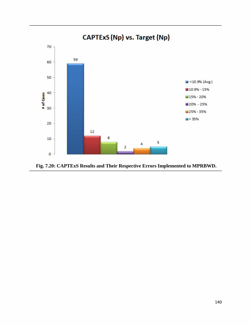
140

Fig. 7.20: CAPTExS Results and Their Respective Errors Implemented to MPRBWD.

141

Fig. 7.21: Comparison Plots of the CAPTExS_Np, Plateau and Abandonment Times versus

their respective Targets Implemented to MPRBWD.

142

7.6.2 Testing Cumulative, Abandonment and Plateau Times Expert

System (CAPTExS) Predictions of Cumulative Gas Production (Gp) Applied

to Multi-Phase Reservoirs with Bottom Water Drive (MPRBWD)

Simultaneously the network was successful in predicting the cumulative gas

productions for the same 90 cases with an overall average error of about ~14%, where 68 cases

with errors less than the overall average as displayed in Figure 7.22. Also the comparison plots

of the same 8 cases are shown in Figure 7.23.

Fig. 7.22: CAPTExS Results and Their Respective Errors Implemented to MPRBWD.

143

Fig. 7.23: Comparison Plots of the CAPTExS_Gp vs. Target_Gp Implemented to

MPRBWD.

144

Chapter 8 Graphical User Interface and Summary

8.1 Integrated Artificial Expert Systems Graphical User Interfaces

(GUIs)

The developed expert systems were compiled and assembled into a tool box that is user

friendly, easy to install and does not require advance knowledge of the artificial neural networks

running in the backgrounds. Without this assembly the benefits of the developed networks would

be limited to those in close communication with the developer for a one on one showcase or

those with background knowledge of how to set up the inputs for the ANNs and how to extract

the results and present them in an informative manner. Therefore, the artificial expert systems

graphical user interfaces are of great importance to the usefulness of the developed networks,

their applicability and popularity. This section will highlight some of the integration and

interactions between the expert systems. The GUIs were created using GUIDE, the MATLAB®

graphical user interface development environment (MATLAB®, 2011).

8.1.1 Main Window

The main window is the portal from which the user starts and selects the function

he/she wants to perform. It first, lists which reservoir type the user would want to address, either

the volumetric single phase gas reservoirs or the multi-phase reservoirs with bottom water drive

as illustrated in Figure 8.1. Clicking on one of the pushbuttons will navigate the engineer to the

desired model. Figure 8.2 is displayed once the volumetric single phase gas reservoirs option is

chosen.

145

Fig. 8.1: Main Window of the Integrated Artificial Expert System Graphical User

Interface (GUI).

146

Fig. 8.2: Main Window of the Volumetric Single Phase Gas Reservoirs Expert System.

147

8.1.2 Reservoir Evaluation Expert System (REExS) GUI in the

Volumetric Single Phase Gas Reservoirs (VSPGR) Model

In this environment the user would want to acquire some reservoir properties. The

input parameters panel lists the editable boxes for entering the production time in units of

months, the observed rates in MMscf/d, and the multi-lateral well design parameters. For simple

illustration default values, that can be modified and saved by the user, are predefined and the

observed rates are plotted and a 3D view of the well as illustrated in Figure 8.3. When the

‘Evaluate’ button in the output parameters panel is pressed it calls the REExS, which collects the

user’s entries from the input parameters panel and produces the required results. Furthermore,

the user has the option to crosscheck these properties by reproducing the rate decline profile

using the predicted properties and compare the new profile to the observed rate decline and

returns the error in the designated box to the far right. The first column to the left under the cross

checking panel will be populated with the rate values generated by the numerical simulator when

the ‘Forecast’ button is clicked, which is the preferred tool to crosscheck with if it is accessible

otherwise the RDExS can be used to regenerate the rates by pressing on the ‘Forecast’ icon

above the right column. In addition, if the user is curious about the long term performance, by

pressing on the button in the middle where it says ‘Plot All’ it will display a 50-year forecast by

using both the numerical simulator, if it’s accessible, and the FExS. The first three pushbuttons

located at the bottom of the window are navigation buttons which can take the user back to either

the main window, to the FExS GUI, or to the MLWDAS GUI respectively and the fourth one is

just a clear button if the user chooses to clear his/her previous inputs and start with a new page.

Figure 8.4 demonstrates the REExS GUI with some examples of the mentioned features.

148

Fig. 8.3: Reservoir Evaluation Expert System (REExS) GUI under VSPGR Environment.

Fig. 8.4: REExS GUI Illustrating Some of its Produced Results.

149

8.1.3 Forecast Expert System (FExS) GUI

The purpose of this GUI is to provide the user with a long term forecast of the

subject reservoir sector by entering basic knowledge of the multi-lateral well design and

reservoir properties under the input parameters panel to the far left of the window as presented in

Figure 8.5. Two forecasting options are available under the output parameters panel. One is

forecasting using the numerical simulator, which should be the primary pick if it is available and

the GUI can interface with it, the other one is forecasting using the developed FExS. Also the

press button ‘Using Both’ will provide the performance results using both tools and the box to

the far right will display the average error percentage.

Fig. 8.5: Forecast Expert System (FExS) GUI under VSPGR Environment.

150

8.1.4 Multi-Lateral Well Design Advisory System (MLWDAS) GUI

Here the user is interested in knowing the design parameters of a well that will

perform according to a predefined target and known reservoir properties. In this GUI that’s

exactly what the user needs to provide. The two columns to the far left shown in Figure 8.6 are

designated for entering the target recovery profile and the reservoir properties respectively.

When the ‘Design The Well’ pushbutton is pressed the design parameters are generated and the

3D schematic of the well appears as in Figure 8.7.

Fig. 8.6: Multi-Lateral Well Design Advisory System (MLWDAS) GUI under VSPGR

Environment.

151

Fig. 8.7: MLWDAS GUI Showing the Well Design Parameters and the 3D View.

Furthermore, the crosschecking mechanism is also available by using the

numerical simulator, priority if available, and the FExS. When either ‘SIM’ or ‘FExS’ or ‘Plot

All’ pushbuttons is selected, the reservoir properties and the recommended multi-lateral well

design parameters will be collected and entered into both engines to generate its respective

recovery profiles forecast. Then the predicted profile will be compared to the target or desired

profile and the error will be measured and displayed to the far right. If ‘Plot All’ is selected the

error box on top shows the error between the target and the numerical simulator prediction; the

second box in the middle is the error between the target and the FExS outputs, and the third one

shows the error between the FExS and the numerical simulator as another crosscheck of the

FExS. These features are illustrated in Figure 8.8.

152

Fig. 8.8: MLWDAS GUI Showing the SIM and the FExS Predictions vs. the Target

Cumulative Percent Recoveries and Corresponding Errors.

153

8.2 Summary

In this dissertation, an approach for developing and employing artificial expert systems in

different petroleum engineering related aspects has been orchestrated. Illustrated the gradual

progression in developing the integrated artificial expert systems for a wide spectrum of

Volumetric Single Phase Gas Reservoirs (VSPGR) and Multi-Phase Reservoirs with Bottom

Water Drive. The forward-looking networks serve as proxies to the numerical simulators when

applicable, hence working as a buffer or a filtration mechanism since the engineer can analyze

and go through many cases in a fraction of the time, labor, and expertise required by the

conventional numerical simulators. This is expected to effectively enhance the efficiency at the

workplace by saving time, efforts and money. Provided the inverse-looking solutions for

predicting parameters for designing multi-lateral wells for a given set of targeted reservoir

performances, and a second network that estimates critical reservoir properties from observed

productions. The inverse-looking solutions are targeted to reduce the uncertainties and guide a

design of a multi-lateral well and provide assistance in history matching problems by minimizing

arbitrarily trial and error approaches and abuse usage of multipliers and modifiers.

The networks are developed in a fashion where they are intertwined and can be used for

crosschecking each other in the absence of a higher fidelity tool. They have been assembled in a

tool box with a user friendly interface to simplify its application without requiring knowledge of

the background mechanism.

However it is emphasized that this dissertation is not suggesting the replacement of existing

and well established procedures, protocols and know-how with the developed expert systems, but

rather applying them as auxiliary, pre-screening or complimentary systems when and where

154

applicable to ease of the computational overload, deliver a solution to the inverse-looking

problems and enhance the overall decision-making process.

8.3 Recommendations

The author, motivated by his committee, recommends expanding on this work by future

researchers, however not limited to these suggestions:

1- Expand to a full-field scale model where more wells are included in a single reservoir

to understand and account for interference between wells.

2- Add economic parameters to multi-lateral well designs that can assist in screening

and optimizing fit for purpose well architecture.

3- Address other reservoir types with different drive mechanisms.

4- Allow flexibility of the expert systems to account for different PVT and relative

permeability tables for different reservoirs with ranging initial and connate

saturations.

5- Designing graphical user interface for the developed expert systems is a powerful

way to attract attention and spark a paradigm shift towards this line of research, hence

increasing the size of enthusiasts will increase the number and improve the quality of

future related studies.

155

References

Ali, J. K., 1994. Neural Networks: A New Tool for the Petroleum Industry?. Aberdeen, U.K.,

European Petroleum Computer Conference, SPE 27561.

Ayala H., L. F. & Ertekin, T., 2007. Neuro-simulation analysis of pressure maintenance

operations in gas condensate reservoirs. Journal of Petroleum Science and Engineering, Volume

58, pp. 207-226.

Bansal, Y., 2011. Forecasting the Production Performance of Wells Located in Tight Oil Plays

Using Artificial Expert Systems (Dissertation), University Park: The Pennsylvania State

University.

Bittencourt, A. C. & Horne, R. N., 1997. Reservoir Development and Design Optimization. San

Antonio, Texas, Annual Technical Conference and Exhibition, SPE 38895.

Chidambaram, P., 2009. Development and Testing of an Artificial Neural Network Based History

Matching Protocol to Characterize Reservoir Properties (Dissertation), University Park: The

Pennsylvania State University.

Dakshindas, S. S., Ertekin, T. & Grader, A. S., 1999. Virtual Well Testing. Charleston, West

Virginia, Eastern Regional Meeting, SPE 57452.

Demuth, H. & Beale, M., 2002. Neural Network Toolbox User's Guide. 13 ed. Natick: The

MathWorks, Inc..

Ertekin, T., Abou-Kassem, J. H. & King, G. R., 2001. Basic Applied Reservoir Simulation.

Richardson: Society of Petroleum Engineers.

156

Garrouch, A. A., Lababidi, H. M. & Ebrahim, A. S., 2005. A web-based expert system for the

planning and completion of multilateral wells. Journal of Petroleum Science and Engineering,

Volume 49, pp. 162-181.

Gharehlo, A. M., 2012. Development of Artificial Expert Reservoir Characterization Tools for

Unconventional Reservoirs (Dissertation), University Park: The Pennsylvania State University.

Graupe, D., 2007. Princeiples of Artificial Neural Networks. 2nd ed. Hackensack: World

Scientific Publishing Co. Pte. Ltd..

Jeirani, Z. & Mohebbi, A., 2006. Estimating the initial pressure, permeability and skin factor of

oil reservoirs using artificial neural networks. Journal of Petroleum Science and Engineering,

Volume 50, pp. 11-20.

McCulloch, W. S. & Pitts, W., 1943. A Logical Calculus of The Ideas Immanent in Nervous

Activity. Bulletin of Mathematical Biology, 5(4), pp. 115-133.

Nelson, A. L., 2012. nelsonrobotics. [Online]

Available at: http://www.nelsonrobotics.org/publications.html

[Accessed 1 August 2012].

Ozkan, E., Yildiz, T. & Kuchuk, F., 1998. Transient Pressure Behavior of Dual-Lateral Wells.

SPE Journal, 3(2), pp. 181-190.

Retnanto, A., Frick, T. P., Brand, C. W. & Economies, M. J., 1996. Optimal Configurations of

Multiple-Lateral Horizontal Wells. Anchorage, USA, Western Regional Meeting, SPE 35712.

Rosenblatt, F., 1957. The Perceptron-a perciving and recognizing automaton, Buffalo: Cornell

Aeronautical Laboratory.

157

Rumelhart, D. E., Hinton, G. E. & Williams, R. J., 1986. Learning representations by back-

propagating errors. Nature, 323(6088), pp. 533-536.

Silpngarmlers, N., Guler, B., Ertekin, T. & Grader, A. S., 2002. Development and Testing of

Two-Phase Relative Permeability Predictors Using Artificial Neural Networks. SPE Journal,

7(3), pp. 299-308.

Thararoop, P., Karpyn, Z., Giman, A. & Ertekin, T., 2008. Integration of seismic attributes and

production data for infill drilling strategies - A virtual intelligence approach. Journal of

Petroleum Science and Engineering, 63(4), pp. 43-52.

Wikimedia Foundation, Inc, 2012. Wikipedia. [Online]

Available at: http://en.wikipedia.org/wiki/Perceptron

[Accessed 1 August 2012].

Yeten, B., Durlofsky, L. J. & Aziz, K., 2003. Optimization of Nonconventional Well Type,

Location, and Trajectory. SPE Journal, 8(3), pp. 200-210.

158

Appendix A

Sample Data Files

A.1 Sample Data File for Volumetric Single Phase Gas Reservoirs

RESULTS SIMULATOR IMEX 200900

INUNIT FIELD

WSRF WELL 1

WSRF GRID TIME

WSRF SECTOR TIME

OUTSRF WELL LAYER NONE

OUTSRF RES ALL

OUTSRF GRID SO SG SW PRES OILPOT BPP SSPRES WINFLUX

WPRN GRID 0

OUTPRN GRID NONE

OUTPRN RES NONE

**$ Distance units: ft

RESULTS XOFFSET 0.0000

RESULTS YOFFSET 0.0000

RESULTS ROTATION 0.0000 **$ (DEGREES)

RESULTS AXES-DIRECTIONS 1.0 -1.0 1.0

**$

**********************************************************************

*****

**$ Definition of fundamental cartesian grid

**$

**********************************************************************

*****

GRID VARI 31 31 10

KDIR DOWN

DI IVAR

31*1.202654e+002

DJ JVAR

31*1.202654e+002

DK ALL

9610*7.349760e+000

DTOP

961*3000

**$ Property: NULL Blocks Max: 1 Min: 1

**$ 0 = null block, 1 = active block

NULL CON 1

**$ Property: Porosity Max: 0.2 Min: 0.2

POR CON 1.374580e-001

**$ Property: Permeability I (md) Max: 0.1 Min: 0.1

PERMI CON 2.208480e-002

159

**$ Property: Permeability J (md) Max: 0.1 Min: 0.1

PERMJ CON 5.263610e-003

**$ Property: Permeability K (md) Max: 0.005 Min: 0.005

PERMK CON 3.060820e-003

**$ Property: Pinchout Array Max: 1 Min: 1

**$ 0 = pinched block, 1 = active block

PINCHOUTARRAY CON 1

CPOR 0.000001

MODEL GASWATER

TRES 150

PVTG EG 1

**$ p Eg visg

14.696 4.81354 0.0113254

247.05 84.1831 0.0116391

479.403 170.17 0.0121176

711.757 263.362 0.0127436

944.11 363.994 0.0135319

1176.46 471.576 0.0145019

1408.82 584.477 0.0156674

1641.17 699.795 0.0170259

1873.52 813.864 0.0185532

2105.88 923.227 0.0202077

2338.23 1025.44 0.0219411

2570.59 1119.27 0.0237088

2802.94 1204.45 0.0254751

3035.29 1281.34 0.0272138

3267.65 1350.61 0.0289078

3500 1413.08 0.0305474

DENSITY GAS 6.438740e-002

REFPW 14.696

DENSITY WATER 61.6381

BWI 1.01944

CW 3.1589e-006

VWI 0.47184

CVW 0.0

ROCKFLUID

RPT 1

SWT

160

**$ Sw krw

.22 0

.3 .07

.4 .15

.5 .24

.6 .33

.8 .65

.9 .83

1 1

SLT

**$ Sl krg

.22 1

.3 .8125

.4 .5

.5 .42

.6 .34

.7 .24

.8 .1

.9 .022

.96 0

1 0

INITIAL

VERTICAL DEPTH_AVE WATER_GAS EQUIL NOTRANZONE

REFDEPTH 3100

REFPRES 3.723190e+003

DWGC 3500

DATUMDEPTH 3100 INITIAL

NUMERICAL

RUN

DATE 1901 1 1

DTWELL 0.1

**$

WELL 'Well-1'

PRODUCER 'Well-1'

OPERATE MIN BHP 500. STOP

MONITOR MIN STG 500000. SHUTIN

**$ rad geofac wfrac skin

GEOMETRY I 0.25 0.37 1. 0.

PERF GEO 'Well-1'

**$ UBA ff Status Connection

18 16 2 1. OPEN FLOW-TO 'SURFACE'

19 16 2 1. OPEN FLOW-TO 1





DATE 1931 1 1.00000

STOP

161

A.2 Sample Data File for Multi-Phase Reservoirs With Bottom

Water Drive

RESULTS SIMULATOR IMEX 200900

INUNIT FIELD

WSRF WELL 1

WSRF GRID TIME

WSRF SECTOR TIME

OUTSRF WELL LAYER NONE

OUTSRF RES ALL

OUTSRF GRID SO SG SW PRES OILPOT BPP SSPRES WINFLUX

WPRN GRID 0

OUTPRN GRID NONE

OUTPRN RES NONE

**$ Distance units: ft

RESULTS XOFFSET 0.0000

RESULTS YOFFSET 0.0000

RESULTS ROTATION 0.0000 **$ (DEGREES)

RESULTS AXES-DIRECTIONS 1.0 -1.0 1.0

**$

**********************************************************************

*****

**$ Definition of fundamental cartesian grid

**$

**********************************************************************

*****

GRID VARI 31 31 10

KDIR DOWN

DI IVAR

31*151

DJ JVAR

31*151

DK ALL

9610*6

DTOP

961*5031

**$ Property: NULL Blocks Max: 1 Min: 1

**$ 0 = null block, 1 = active block

NULL CON 1

**$ Property: Porosity Max: 0.2 Min: 0.2

POR CON 1.500000e-001

**$ Property: Permeability I (md) Max: 0.1 Min: 0.1

PERMI CON 236

**$ Property: Permeability J (md) Max: 0.1 Min: 0.1

PERMJ CON 164

**$ Property: Permeability K (md) Max: 0.005 Min: 0.005

PERMK CON 1.640000e+001

AQUIFER BOTTOM

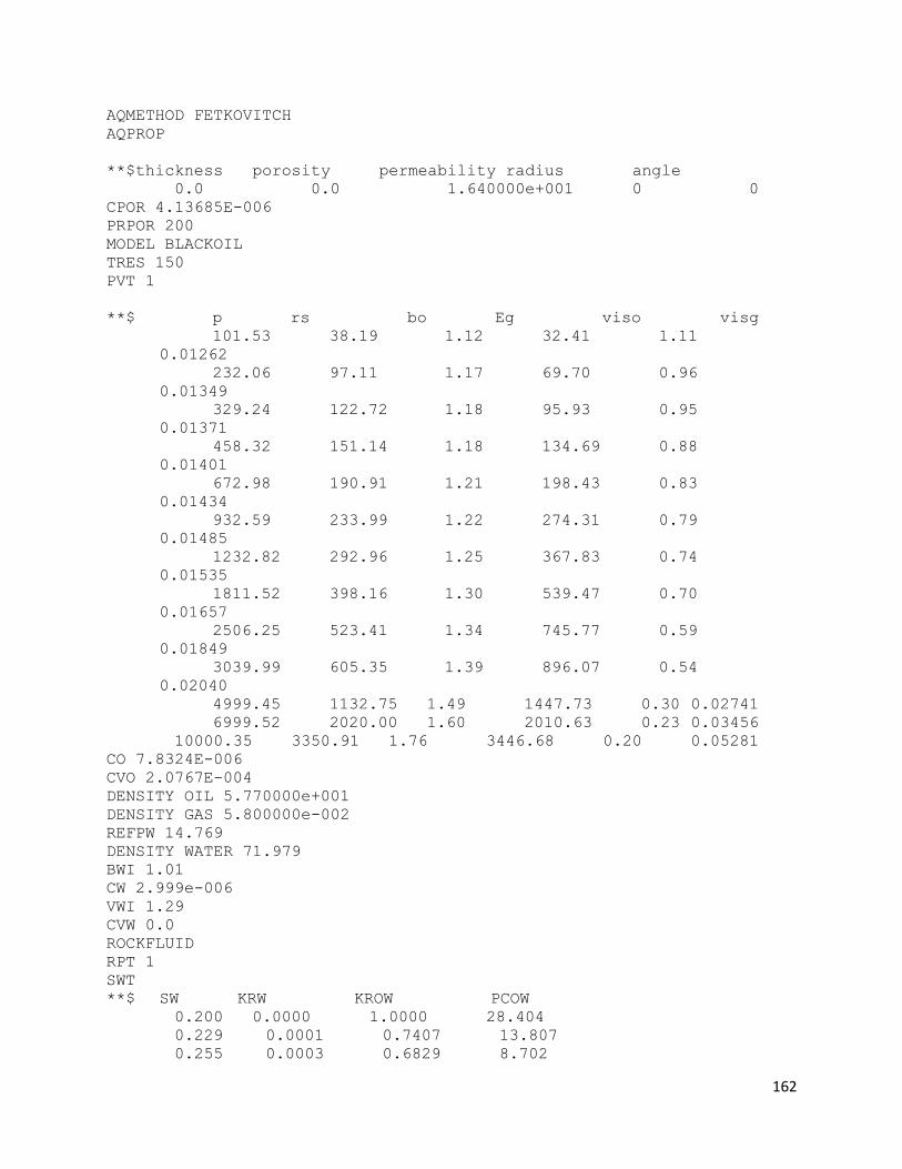
162

AQMETHOD FETKOVITCH

AQPROP

**$thickness porosity permeability radius angle

0.0 0.0 1.640000e+001 0 0

CPOR 4.13685E-006

PRPOR 200

MODEL BLACKOIL

TRES 150

PVT 1

**$ p rs bo Eg viso visg

101.53 38.19 1.12 32.41 1.11

0.01262

232.06 97.11 1.17 69.70 0.96

0.01349

329.24 122.72 1.18 95.93 0.95

0.01371

458.32 151.14 1.18 134.69 0.88

0.01401

672.98 190.91 1.21 198.43 0.83

0.01434

932.59 233.99 1.22 274.31 0.79

0.01485

1232.82 292.96 1.25 367.83 0.74

0.01535

1811.52 398.16 1.30 539.47 0.70

0.01657

2506.25 523.41 1.34 745.77 0.59

0.01849

3039.99 605.35 1.39 896.07 0.54

0.02040

4999.45 1132.75 1.49 1447.73 0.30 0.02741

6999.52 2020.00 1.60 2010.63 0.23 0.03456

10000.35 3350.91 1.76 3446.68 0.20 0.05281

CO 7.8324E-006

CVO 2.0767E-004

DENSITY OIL 5.770000e+001

DENSITY GAS 5.800000e-002

REFPW 14.769

DENSITY WATER 71.979

BWI 1.01

CW 2.999e-006

VWI 1.29

CVW 0.0

ROCKFLUID

RPT 1

SWT

**$ SW KRW KROW PCOW

0.200 0.0000 1.0000 28.404

0.229 0.0001 0.7407 13.807

0.255 0.0003 0.6829 8.702

163

0.308 0.0012 0.5722 3.190

0.334 0.0023 0.5194 2.726

0.412 0.0102 0.3715 1.827

0.464 0.0219 0.1526 1.222

0.557 0.0416 0.0822 0.638

0.606 0.0721 0.0000 0.191

0.647 0.1448 0.0000 0.000

0.700 0.1780 0.0000 0.000

0.800 0.2604 0.0000 0.000

1.000 1.0000 0.0000 0.000

SLT

**$ SL KRG KROG PCOG

0.200 1.0000 0.0000 564.429

0.316 0.6784 0.0000 84.064

0.435 0.6215 0.0000 54.012

0.562 0.5456 0.0000 35.172

0.614 0.3939 0.0020 8.818

0.702 0.1399 0.0280 5.397

0.812 0.0515 0.1721 1.980

0.875 0.0297 0.3395 1.516

0.906 0.0226 0.4395 1.305

0.937 0.0173 0.5500 1.089

0.969 0.0131 0.6702 0.856

1.000 0.0000 1.0000 0.000

INITIAL

VERTICAL BLOCK_CENTER WATER_OIL_GAS

PB CON 2189

REFDEPTH 5061

REFPRES 2189

DGOC 5025

DWOC 5121

NUMERICAL

RUN

DATE 2013 1 1

DTWELL .04167

**$

WELL 'Well-1'

PRODUCER 'Well-1'

OPERATE MAX STO 6000 CONT

OPERATE MIN BHP 14.7 *CONT

MONITOR MIN STO 50.0 SHUTIN

MONITOR MAX GOR 4000.0 SHUTIN

MONITOR MAX WCUT 0.99 SHUTIN

**$ rad geofac wfrac skin

GEOMETRY I 0.25 0.37 1. 0.

PERF GEO 'Well-1'

**$ UBA ff Status Connection

15 16 6 1. OPEN FLOW-TO 'SURFACE'


164









20 16 2 1. OPEN FLOW-TO 10


16 14 8 1. OPEN FLOW-TO 12

16 13 8 1. OPEN FLOW-TO 13

16 12 8 1. OPEN FLOW-TO 14

16 11 8 1. OPEN FLOW-TO 15

16 10 8 1. OPEN FLOW-TO 16

DATE 2014 1 1.00000

DATE 2016 1 1.00000

DATE 2018 1 1.00000

DATE 2020 1 1.00000

DATE 2022 1 1.00000

DATE 2024 1 1.00000

DATE 2026 1 1.00000

DATE 2028 1 1.00000

DATE 2030 1 1.00000

DATE 2032 1 1.00000

DATE 2034 1 1.00000

DATE 2036 1 1.00000

DATE 2038 1 1.00000

DATE 2040 1 1.00000

DATE 2042 1 1.00000

DATE 2044 1 1.00000

DATE 2046 1 1.00000

DATE 2048 1 1.00000

DATE 2050 1 1.00000

DATE 2052 1 1.00000

DATE 2054 1 1.00000

DATE 2056 1 1.00000

DATE 2058 1 1.00000

DATE 2060 1 1.00000

DATE 2062 1 1.00000

DATE 2072 1 1.00000

DATE 2083 1 1.00000

STOP

Vitae

Talal Saeed AlMousa

Talal was born in Riyadh, Saudi Arabia in October of 1976, the eldest of 8 brothers and

six sisters. He joined Saudi Aramco in August of 1995 immediately after high school. A year

later, the company awarded him a scholarship to the United States where he attended Louisiana

State University (LSU), Baton Rouge, Louisiana, for five semesters (08/96 – 12/98). He then

transferred to King Fahd University of Petroleum and Minerals (KFUPM), Dhahran, Saudi

Arabia, where he earned his Bachelor’s of Science degree in petroleum engineering in 2002.

In July 2002 Talal joined Saudi Aramco’s workforce as a reservoir management engineer

and became a member in the Society of Petroleum Engineers (SPE). As part of his development

plan, in July 2003 Talal was assigned to work as a log analyst with reservoir description group.

In January 2004 he assumed drilling engineer responsibilities with deep gas drilling division.

Then he worked as a production engineer for one year from 07/04 – 06/05. In July 2005 Talal

returned to reservoir management department where he had the opportunity to manage mature

fields, participate in the development of a new increment and author and co-author two SPE

papers in the area of production engineering and rock mechanics.

Talal enrolled at KFUPM as a part-time graduate student in August 2005 while holding a

fulltime job as a reservoir engineer with Saudi Aramco. He earned his Master’s of Science

degree in petroleum engineering in June 2008. Talal was elected to join the Technologist

Development Program (TDP), an in house program designed by Saudi Aramco, to achieve

specialist status in reservoir management of intelligent fields. In August 2009 Talal was granted

a second scholarship by Saudi Aramco to attend the Ph.D. program at The Pennsylvania State

University (PSU). He successfully defended his dissertation on June 24, 2013 and earned his

Doctoral degree in energy and mineral engineering with option in petroleum and natural gas

engineering in August 2013. Soon after his graduation he resumed his role with Saudi Aramco in

Dhahran, Saudi Arabia as a reservoir management engineer. He can be reached any time at

[email protected].

mailto:[email protected]

development and utilization of integrated artificial

Documents