Title: A memory-integrated artificial bee algorithm for heuristic optimisation Name: T. Bayraktar

This is a digitised version of a dissertation submitted to the University of Bedfordshire.

It is available to view only.

This item is subject to copyright.

1

A MEMORY-INTEGRATED ARTIFICIAL BEE ALGORITHM

FOR HEURISTIC OPTIMISATION

T. BAYRAKTAR

MSc. by Research

2014

UNIVERSITY OF BEDFORDSHIRE

2

A MEMORY-INTEGRATED ARTIFICIAL BEE ALGORITHM FOR HEURISTIC

OPTIMISATION

by

T. BAYRAKTAR

A thesis submitted to the University of Bedfordshire in partial fulfilment of the

requirements for the degree of Master of Science by Research

February 2014

3

A MEMORY-INTEGRATED ARTIFICIAL BEE ALGORITHM FOR HEURISTIC OPTIMISATION

T. BAYRAKTAR

ABSTRACT

According to studies about bee swarms, they use special techniques for foraging and they are always

able to find notified food sources with exact coordinates. In order to succeed in food source

exploration, the information about food sources is transferred between employed bees and onlooker

bees via waggle dance. In this study, bee colony behaviours are imitated for further search in one of

the common real world problems. Traditional solution techniques from literature may not obtain

sufficient results; therefore other techniques have become essential for food source exploration. In

this study, artificial bee colony (ABC) algorithm is used as a base to fulfil this purpose. When

employed and onlooker bees are searching for better food sources, they just memorize the current

sources and if they find better one, they erase the all information about the previous best food source.

In this case, worker bees may visit same food source repeatedly and this circumstance causes a hill

climbing in search. The purpose of this study is exploring how to embed a memory system in ABC

algorithm to avoid mentioned repetition. In order to fulfil this intention, a structure of Tabu Search

method -Tabu List- is applied to develop a memory system. In this study, we expect that a memory

system embedded ABC algorithm provides a further search in feasible area to obtain global optimum

or obtain better results in comparison with classic ABC algorithm. Results show that, memory idea

needs to be improved to fulfil the purpose of this study. On the other hand, proposed memory idea

can be integrated other algorithms or problem types to observe difference.

4

DECLARATION

I declare that this thesis is my own unaided work. It is being submitted for the degree of

Master of Science by Research at the University of Bedfordshire.

It has not been submitted before for any degree or examination in any other University.

Name of candidate: Signature:

Date:

5

LIST OF ABBREVIATION AND ACRONYMS

ABC : Artificial Bee Colony

BF : Best Fit

BFD : Best Fit Decreasing

BP : Bin Packing

Et al : And others

FF : First Fit

Fig : Figure

MEABC : Memory Embedded Artificial Bee Colony

NF : Next Fit

NP : Non-deterministic Polynomial

STTL : Short Term Tabu List

WF : Worst Fit

LIST OF SYMBOLS IN EQUATIONS

H : Hessian Matrix

∂² : Second Partial Differential

X : Solution Value

U : Upper Bound for a Solution Parameter

L : Lower Bound for a Solution Parameter

V : Possible Solutions in Neighbourhood Area of Current Solution Value X

Ø : Random Real Value Between -1 and +1

Abs : Absolute Value

P : Probability Value for a Solution Value X to be Chosen

∑ : Summation

SN : Size of the Initial Population

Rand : Random Real Value between 0 and +1

6

Table of Contents

Abstract .................................................................................................................................................. 3

List of Abbreviation and Acronyms ....................................................................................................... 5

List of Symbols in Equations .................................................................................................................. 5

Table of Contents ................................................................................................................................... 6

List of Figures and Tables ....................................................................................................................... 8

Chapter 1: Introduction ........................................................................................................................ 11

1.1 Collective Behaviours and Swarm Intelligence ............................................................................. 12

1.2 Proposed Algorithm ....................................................................................................................... 13

1.2.1 Aim and Objectives ..................................................................................................................... 13

1.2.2 Methodology ............................................................................................................................... 13

Chapter 2: Literature Review ............................................................................................................... 15

2.1 Deterministic Optimisation ............................................................................................................ 17

2.2 Calculation Difficulties in Newton Search Method ....................................................................... 19

2.3 Heuristic Optimisation ................................................................................................................... 20

2.3.1 Evolutionary Computation .......................................................................................................... 24

2.3.1.1 Genetic Algorithm .................................................................................................................... 24

2.3.1.2 Evolution Strategies and Evolutionary Programming ............................................................. 25

2.3.1.3 Differential Evolution ............................................................................................................... 26

2.3.2 Swarm Intelligence ...................................................................................................................... 26

2.3.2.1 Particle Swarm Optimisation ................................................................................................... 26

2.3.2.2 Ant Colony Search Algorithm ................................................................................................... 27

2.3.2.3 Artificial Bee Colony (ABC) Algorithm ..................................................................................... 28

2.3.2.3.1 Formulation of ABC Algorithm ............................................................................................. 33

2.3.3 Individual Solution Driven Heuristic Algorithms ........................................................................ 36

2.3.3.1 Simulated Annealing ................................................................................................................ 36

2.3.3.2 Tabu Search Method ................................................................................................................ 37

2.4 Bin Packing Problems ..................................................................................................................... 41

2.4.1 One Dimensional (1D) Bin Packing Problems ............................................................................. 42

2.4.2 Two and Three Dimensional (2D & 3D) Bin Packing Problems .................................................. 44

7

Chapter 3: Proposed Approach ............................................................................................................ 46

3.1 Fundamental Concepts of Proposed Approach ............................................................................. 46

3.2 Implementation of Proposed Approach ........................................................................................ 47

3.2.1 Problem Representation and Neighbourhood Structure .......................................................... 47

3.2.2 Bin Loading Method .................................................................................................................... 48

3.2.3 Generating a New Solution ......................................................................................................... 49

3.2.4 The Roulette Wheel Function ..................................................................................................... 51

3.2.5 Enhancement with Memory ....................................................................................................... 51

3.2.6 A Software Implementation for Proposed Algorithm ............................................................... 52

Chapter 4: Experimental Results and Discussion ................................................................................ 55

4.1 Datasets .......................................................................................................................................... 55

4.2 Parameter Settings ......................................................................................................................... 55

4.3 Experimental Results…………………………………………………………………………………………...……………………61

4.3.1 Results for Traditional Algorithms…………………………………………………………………...……………………61

4.3.2 Results for Artificial Bee Colony (ABC) Algorithm.…………………………………………...……………………63

4.3.3 Results for Memory Embedded Artificial Bee Colony (MEABC) Algorithm ……...……………………68

Chapter 5: Conclusion .......................................................................................................................... 76

References ............................................................................................................................................ 79

Appendix A ........................................................................................................................................... 83

Appendix B ……...…………………………………………………………………………………………………………………………….92

Appendix C ……………………………………………………………………………………………………. ……...……………………126

8

List of Figures and Tables

Fig. 1.A: Convex Set .............................................................................................................................. 16

Fig. 1.B: Non-Convex Set ....................................................................................................................... 16

Fig. 2: Branches of Optimisation Problems ........................................................................................... 17

Fig. 3: The Waggle Dance Performed by Honey Bees .......................................................................... 31

Fig. 4: The behaviour of honey bee foraging for nectar ...................................................................... 32

Fig. 5: Classic ABC Algorithm……………………………………………………………………………………………………………35

Fig. 6: Artificial Bee Colony (ABC) Algorithm Flowchart ...................................................................... 36

Fig. 7: Tabu Search Based on Short Term Tabu List .............................................................................. 40

Fig. 8: Packing Under Next Fit Algorithm ............................................................................................. 42

Fig. 9: Packing Under First Fit Algorithm .............................................................................................. 43

Fig. 10: Packing Under Best Fit Algorithm ............................................................................................ 43

Fig. 11: Packing Under Worst Fit Algorithm ......................................................................................... 44

Fig. 12: Packing Under First-Best Fit Decreasing Algorithm ................................................................. 44

Fig. 13: Raw Assignation Result of Item-set Example in First Step ....................................................... 48

Fig. 14: The Result of Combination Process.......................................................................................... 49

Fig. 15: Modified Result of Assignation for Items ................................................................................. 49

Fig. 16: Generating a New Solution ...................................................................................................... 50

Fig. 17: Modification of Generated Solution ........................................................................................ 50

Fig. 18: The Modified New Solution ..................................................................................................... 51

Fig. 19.A: Window for Traditional Algorithms ...................................................................................... 53

Fig. 19.B: Window for ABC Algorithm ................................................................................................... 54

Fig. 19.C: Window for Proposed Algorithm .......................................................................................... 54

Fig. 20.A: 5000 Iteration Experiment for Dataset-4 Group-7 ............................................................... 58

Fig. 20.B: 7500 Iteration Experiment for Dataset-4 Group-7 ............................................................... 58

Fig. 20.C: 10000 Iteration Experiment for Dataset-4 Group-7 ............................................................. 59

Fig. 21.A: 100 Failure Experiment for Dataset-4 Group-7 .................................................................... 60

Fig. 21.B: 1,000 Failure Allowance Experiment for Dataset-4 Group-7 ................................................ 60

Fig. 22.A: Average Number of Bins Graph for Table 5.A ...................................................................... 63

Fig. 22.B: Average Wastage Graph for Table 5.A .................................................................................. 63

Fig. 23.A: Average Number of Bins Graph for Table 5.B ....................................................................... 64

Fig. 23.B: Average Wastage Graph for Table 5.B .................................................................................. 64

Fig. 24.A: Average Number of Bins Graph for IS-3 in Table 5.C ............................................................ 65

9

Fig. 24.B: Average Wastage Graph for IS-3 in Table 5.C ....................................................................... 65

Fig. 25.A: Average Number of Bins Graph for IS-4 in Table 5.C ............................................................ 65

Fig. 25.B: Average Wastage Graph for IS-4 in Table 5.C ....................................................................... 65

Fig. 26.A: Average Number of Bins Graph for Table 5.D ...................................................................... 66

Fig. 26.B: Average Wastage Graph for Table 5.D.................................................................................. 66

Fig. 27.A: Average Number of Bins Graph for Table 5.E ....................................................................... 67

Fig. 27.B: Average Wastage Graph for Table 5.E .................................................................................. 67

Fig. 28.A: Average Number of Bins Graph for Table 5.F ....................................................................... 67

Fig. 28.B: Average Wastage Graph for Table 5.F .................................................................................. 67

Fig. 29.A: Average Number of Bins Graph for IS8 in Table 5C .............................................................. 68

Fig. 29.B: Average Wastage Graph for IS8 in Table 5C ......................................................................... 68

Fig. 30.A: Average Number of Bins Graph for Table 6.A ...................................................................... 69

Fig. 30.B: AverageWastage Graph for Table 6.A ................................................................................... 69

Fig. 31.A: Average Number of Bins Graph for Table 6.B ....................................................................... 70

Fig. 31.B: AverageWastage Graph for Table 6.B ................................................................................... 70

Fig. 32.A: Average Number of Bins Graph for IS3 in Table 6.C ............................................................. 70

Fig. 32.B: Average Wastage Graph for IS3 in Table 6.C ........................................................................ 70

Fig. 33.A: Average Number of Bins Graph for IS4 in Table 6.C ............................................................. 71

Fig. 33.B: Average Wastage Graph for IS4 in Table 6.C ........................................................................ 71

Fig. 34.A: Average Number of Bins Graph for Table 6.D ...................................................................... 71

Fig. 34.B: AverageWastage Graph for Table 6.D .................................................................................. 71

Fig. 35.A: Average Number of Bins Graph for Table 6.E ....................................................................... 72

Fig. 35.B: AverageWastage Graph for Table 6.E ................................................................................... 72

Fig. 36.A: Average Number of Bins Graph for Table 6.F ....................................................................... 73

Fig. 36.B: AverageWastage Graph for Table 6.F ................................................................................... 73

Fig. 37.A: Average Number of Bins Graph for IS8 in Table 6.C ............................................................. 73

Fig. 37.B: Average Wastage Graph for IS8 in Table 6.C ........................................................................ 73

Table 1: Experiment Results for Dataset-4 Group-7 ............................................................................. 56

Table 2: Experiment Results for Dataset-4 Group-1 ............................................................................. 56

Table 3: The Effect of the Number of Failure Allowance in Same Group in Dataset-4 ........................ 59

Table 4.A: Results of Traditional 1-D Bin Packing Algorithms for Itemset-4 ........................................ 62

Table 4.B: Results of Traditional 1-D Bin Packing Algorithms for Itemset-8 ........................................ 62

Table 5.A: Results of Classic ABC Algorithm for Itemset-1 Group-1 ..................................................... 63

10

Table 5.B: Results of Classic ABC Algorithm for Itemset-2 Group-5 ..................................................... 64

Table 5.C: Results of Classic ABC Algorithm for Itemset-3, Itemset-4, and Itemset-8 ......................... 64

Table 5.D: Results of Classic ABC Algorithm for Itemset-5 Group-2 .................................................... 66

Table 5.E: Results of Classic ABC Algorithm for Itemset-6 Group-2 ..................................................... 66

Table 5.F: Results of Classic ABC Algorithm for Itemset-7 Group-1 ..................................................... 67

Table 6.A: Results of Memory Embedded ABC Algorithm for Itemset-1 Group-1 ............................... 69

Table 6.B: Results of Memory Embedded ABC Algorithm for Itemset-2 Group-5 ............................... 69

Table 6.C: Results of Memory Embedded ABC Algorithm for Itemset-3, Itemset-4, and Itemset-8 .... 70

Table 6.D: Results of Memory Embedded ABC Algorithm for Itemset-5 Group-2 ............................... 71

Table 6.E: Results of Memory Embedded ABC Algorithm for Itemset-6 Group-2 ............................... 72

Table 6.F: Results of Memory Embedded ABC Algorithm for Itemset-7 Group-1 ................................ 72

11

Chapter 1: Introduction

Problem solving has been a challenging area of research for some time. Deterministic methods

which are used for searching for global optimum tend to obtain an exact solution which usually

requires too much time, money and manpower. Prior target for any establishment is optimising the

requirement for these three main resources. More importantly, they usually disregard parameters of

problem sets and consider rather abstract models in problem solving whereas, in real life, most of

the problems do not require exact solutions due to the difficulties obstructing implementation of the

exact solution. Thus, the solutions should be rather flexible to tolerate sudden changes in

circumstances. Heuristic search methods are more suitable for solving real life problems because

they do not require an exact solution. They just propose a variety of approaches to approximate the

exact solution.

A heuristic search method requires the following steps. Firstly, the problem should be defined with a

finite set of search space, decision variables, objective function, and feasible function to be able to

obtain optimum value of the objective function. Secondly, a neighbourhood function should be

defined to search through a local neighbourhood within the search space. A search method is

designed to find a feasible solution within the neighbourhood of a feasible solution area and to

make a decision whether or not to move to the new solution by applying one of the heuristic search

algorithms such as Hill-Climbing, Simulated Annealing, Tabu Search, Genetic Algorithm, Artificial Bee

Colony Algorithm.

In this study, one of the aforementioned heuristic methods is applied for a kind of combinatorial

non-deterministic polynomial (NP)-hard problem known as a bin packing problem, which aims to fill

bins with different objects due to the dimensional relation between them.

The main purpose of bin packing problems is using an area for stocks in a facility as small as possible

to reduce the stocking cost. In order to avoid area wastage, firstly we need to define object and

repositories such as bin, container. There are many variations of this problem, such as 1 or 2 or 3-D

packing problems, packing by weight or cost, loading trucks by weight. There are not only induction

based packing problem examples. There are also many deduction based packing problems such as

cutting stock problems.

12

Researchers may need to answer some questions such as if applied algorithm is compatible with

tackled problems (deterministic or non-deterministic) or not and if they really need to develop an

algorithm or not. For example deterministic problems may not require a kind of developing

algorithm process due to their structure. On the other hand, they need to consider and define

requirements of tackled problems. In this way, they can find suitable algorithms for the solution of

tackled problems. In this study, we also considered classic algorithms with their performance and

results for comparison with developed algorithms.

1.1 Collective Behaviours and Swarm Intelligence

Most creatures, especially tiny sized animals, have to be in cooperation with the same gender in

nature in order to overcome various difficulties due to their handicaps such as their weaknesses in

comparison with other genders and stocking problems for foraged food. If some members of any

gender among creatures come together to benefit from each other’s capacity or energy for any

purpose, this form is called a “swarm”. Swarms in nature have rules to maximize the benefit from

resources and protect the reasonable condition of the swarm system.

Mankind has been inspired by nature to make several developments and innovations throughout

history. Optimisation researchers are also inspired by swarm intelligence and imitate this to develop

several algorithms to obtain or approximate the best solutions for some problems they tackle.

Basically, researchers apply techniques based on swarm intelligence step by step. In this study, we

use techniques especially based on insect (bee) behaviours and try to understand the intelligence

behind these behaviours. Insects apply complex algorithms to overcome problems in nature and this

speciality shows us an alternative way about how to reach an optimum solution. All studies about

swarm behaviours and intelligence reveal the wonderful systems in creatures’ lives. As

aforementioned in this study, bee swarm intelligence and behaviours will assist us in developing an

algorithm.

Artificial Bee Colony (ABC) Algorithm is a bio-inspired population-based heuristic search method

simulating behaviours of honey bees. The algorithm is a recently implemented heuristic algorithm

which briefly works as follows: Initially, half of the colony is recruited as active bees and the other

half as the onlooker bees. Active bees are responsible for foraging and gathering information to

share with onlooker bees. When the amount of food, which is provided by active bees, decreases to

an insufficient level, the active bees proceed to forage without sharing information or abandoning

the food and become scout bees. Based on the information on existing food sources shared by active

bees, inactive bees may also start foraging.

13

1.2 Proposed Algorithm

The main disadvantage of the artificial bee colony algorithm is that bees search for a food supplier

and memorize a resource until they find a better one. In this situation, they may visit the same

resources repeatedly and it is a kind of hill climbing which is known as one of the main threats during

optimum searching because in case hill climbing fails in local optimum curve we would never reach

the main goal of search. In this section, we will describe what stimulates us to develop a hybrid

algorithm and how to overcome the threat mentioned above.

1.2.1 Aim and Objectives

The aim of this research is to investigate how a memory mechanism can be embedded in bee

algorithms so that the bee colonies are enabled to remember their past experiences, and be

sensitive to search within other neighbourhoods. The main reason for using a memory mechanism is

that, search for global optimum may fall in a local optimum and may not escape from there. This

condition is a typical example for fail of hill climbing in a local optimum. For this purpose the tabu list

idea is borrowed from the tabu search algorithm [1] and is integrated into Bee algorithms to help

improve the search performance. In this way, we may constrain the search not to test solutions in

local optimum and search may escape from there by testing other solutions from outside of local

optimum.

The objectives are:

To find out if a memory can be integrated into bee algorithms

To investigate how a memory can improve the efficiency of a bee algorithm

To find out if a tabu list is a good memory mechanism for bee algorithms

To reveal the circumstances in which memory can work better with bee algorithms

To demonstrate if memory-embedded bee algorithms can solve one-dimensional bin-packing

problems better.

1.2.2 Methodology

A classical bee algorithm is considered as the starting point of this research, where it is applied to a

one-dimensional bin-packing problem. The behaviours of such an algorithm will be revealed through

a literature search as well as experimental study. It will be focused on how quick such a bee

algorithm traps local optima and subject to which circumstances. Once this step is completed, the

memory mechanisms will be investigated to make the bees more conscious and able to use past

14

experiences. Tabu search is one of the metaheuristic algorithms that use memory mechanisms to

diversify its search [2]. It requires harvesting neighbour solutions and moves from the current

solution to the best harvested ones subject to a memory mechanism. The memory mechanism is

called a tabu list, which is dynamically updated throughout the search. The main idea of a tabu list is

that once a move is decided it is immediately considered as a tabu move for a period of time, and

then is released. This restriction is expected to help bees included in the search mechanism of bee

algorithms to be more decisive in their search. There will be further investigation on how this idea

would incorporate with bee algorithms for better performance in solving a one-dimensional bin-

packing problem. An extensive experimental study will be conducted to measure the performance

of the variants of this integration and to set up parametric configuration of the algorithms.

The rest of this study is classified into four other chapters. Brief descriptions of the chapters are

provided below to make clear how to develop the proposed algorithm of the study. Besides, a

comparison between classic algorithms and the proposed algorithm is also provided to evaluate

developed algorithm performance.

Chapter 2: This chapter includes all background information about the study, referring to reputable

and reliable sources such as Applied Soft Computing, Information Sciences, European Journal of

Operational Research and other scientific community web sources.

Chapter 3: In this chapter, a proposed solution with necessary techniques and algorithms is

introduced after explanation of classic algorithm implementations in chapter 2 because the new

algorithm is built on this theme. Both classic and newly developed algorithms are analyzed to

present the fitness performance difference between them.

Chapter 4: After description of classic algorithms and introduction of the proposed algorithm in

chapter 2 and chapter 3, they are implemented on several 1-D bin packing problem variable

databases. In this study, MATLAB 2012 software is used for implementations. After implementations

of every single database with different algorithms, results belonging to classic algorithms, modern

algorithms and the newly developed algorithm are compared with discussion about testing

techniques.

Chapter 5: The final chapter will conclude with a brief discussion about the findings of the study and

a summary of the entire study with possible future works.

15

Chapter 2: Literature Review

Optimisation research has been a rapidly growing area of engineering, mathematical science,

computer science and management for the last few decades. The main reasons for this growth are

the high cost of wastage of resources which have some limitations for use and rising demands. All

optimisation problems are about minimizing the wastage to benefit resources completely and

maximizing the output of processes we tackle. Inputs and outputs of processes have different

limitations which lead researchers to propose ideas about finding the best solution to these different

processes; in other words, problems in a feasible area that are defined by these limitations.

Before solving a problem there should be a clear definition of it because the characteristics of

problems lead the way to possible solutions. After definition, the path to solve the problems, in

other words methods/algorithms, needs to be applied to find an optimum or near optimum solution

for the system.

Researchers expect a few unique characteristics, which are aligned respectively as five-bullet-point,

from applied optimisation methods/algorithms:

Tackled methods/algorithms would not fall into local optimum

Competitive computational time in comparison with others

They could be implemented in general purpose computer algebra systems

They could be applied to a wide range of deterministic or non-deterministic problems

They could be combined with other methods/algorithms to increase the efficiency [3]

Problem sets firstly can be divided due to their convexity characteristics in the optimisation area.

If the feasible area/set where variables of the problem set are placed has a convex shape, in which

any two variables can be connected directly without the line between them exceeding the field, it is

called a convex set and searching for the optimum in the convex set is called convex optimisation.

If one of the variable pairs cannot be connected directly as defined above, it is called a non-convex

set and the name for searching for the optimum in this set is called non-convex optimisation. The

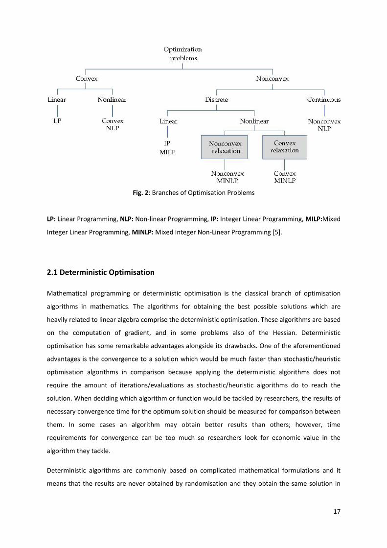
shapes of the convex and non-convex set are shown as in Fig. 1.A and Fig. 1.B. [57]

16

In addition to the problem of subdivision due to their convexity characteristics, there are two kinds

of problems due to whether they tackle decimal or integer variables which are discrete and

continuous problems [59].

Fig. 1.A: Convex Set Fig. 1.B: Non-Convex Set

While tackling continuous problems, the solution searching (feasible) area for optima consists of real

numbers. In this circumstance, any solution can be found in the whole searching area. This means

that, obtaining a better solution has a high possibility rate with all facets of the searching area.

Mathematical optimisation problems are such a good example of continuous problems [59].

On the other hand, while tackling discrete problems, the feasible area consists of integer numbers,

so the solution is also an integer. This circumstance restricts the search in feasible areas and may

give us a lower possibility of obtaining a better solution which can be between two integer solutions

and it is unacceptable for discrete problems. For example, combinatorial optimisation problems are

a branch of discrete problems [59].

There is another and final subdivision for optimisation due to linearity characteristics of objective

functions. If none of the variables of the objective function are quadratic, polynomial or high degree,

this objective function is called a linear function. Otherwise, it is called a non-linear function. Fig.-2

shows the subdivision of optimisation problems by characteristics [5].

After the definition of the type of tackled problems, researchers search for the easiest and the best

way to solve problems and find the optimum/optima. Many researchers have been trying different

and better optimisation techniques to obtain the best solutions or approximate them. Mainly, there

are two kinds of research technique to converge to the optimum/optima which are deterministic

optimisation (mathematical programming) and heuristic optimisation [4].

17

Fig. 2: Branches of Optimisation Problems

LP: Linear Programming, NLP: Non-linear Programming, IP: Integer Linear Programming, MILP:Mixed

Integer Linear Programming, MINLP: Mixed Integer Non-Linear Programming [5].

2.1 Deterministic Optimisation

Mathematical programming or deterministic optimisation is the classical branch of optimisation

algorithms in mathematics. The algorithms for obtaining the best possible solutions which are

heavily related to linear algebra comprise the deterministic optimisation. These algorithms are based

on the computation of gradient, and in some problems also of the Hessian. Deterministic

optimisation has some remarkable advantages alongside its drawbacks. One of the aforementioned

advantages is the convergence to a solution which would be much faster than stochastic/heuristic

optimisation algorithms in comparison because applying the deterministic algorithms does not

require the amount of iterations/evaluations as stochastic/heuristic algorithms do to reach the

solution. When deciding which algorithm or function would be tackled by researchers, the results of

necessary convergence time for the optimum solution should be measured for comparison between

them. In some cases an algorithm may obtain better results than others; however, time

requirements for convergence can be too much so researchers look for economic value in the

algorithm they tackle.

Deterministic algorithms are commonly based on complicated mathematical formulations and it

means that the results are never obtained by randomisation and they obtain the same solution in

18

each run. This fact could be true also for stochastic/heuristic algorithms, however these algorithms

are based on randomisation and they may obtain different solutions in each run [4].

Most researchers find heuristic approaches more flexible and efficient than deterministic methods

which commonly take advantage of analytical properties of the problem; however, many

optimisation problems consist of complicated elements beside their analytical aspects. The quality of

the obtained solutions may not always be sufficient. One of the stochastic/heuristic approach

drawbacks is reduction in the probability of finding a global optimum while searching in big size

problems. Conversely, deterministic approaches can provide general tools for solving optimisation

problems to obtain a global or approximately global optimum which is a solution that a function

reaches highest or lowest value, depending on problem, by using it [5].

Many different fields in optimisation problems would apply to deterministic optimisation.

Skiborowski et al. [6] developed a hybrid optimisation approach based on one of the necessary

attributes of applied methods/algorithms which is combinational flexibility in process design. They

also applied the traditional deterministic optimisation algorithm as a second phase using the results

data of the first phase, which is processed by an evolutionary algorithm in a case study.

Marcovecchio and Novais [7] developed a mixed integer quadratic programming problem (MIQP)

model with a deterministic optimisation approach and apply it to the unit commitment (UC) problem

which has NP-Hard characteristics. In [7], the unit commitment problem is applied for a case study

about reliable power production as a most critical decision process for a large number of interacting

factors. Trindade and Ambrosio [8] proposed one of the deterministic optimisation methods that can

provide some qualified estimates for segment characteristics in the latent segment model when only

aggregate store level data is available. In [8], the storage system works dynamically, so they test the

Sequential Quadratic Programming (SQP) method which is a branch of deterministic optimisation

and accept it as a model fit for estimation in the case study. Sulaiman et al. [9] used a deterministic

method approach to improve the power density of the existing motor used in hybrid electric vehicles

(HEV) and they implement the proposed deterministic method on hybrid excitation flux switching

motor (HEFSM) as a candidate.

Bin packing problems, the main theme of this study, are also applicable for deterministic methods.

Valéiro de Carvalho [10] compared several linear programming (LP) formulations for the 1-D cutting

stock and bin packing problems via different algorithms. Carvalho used results from experiments

belonging to the mentioned algorithms to analyze characteristics and determine the best algorithm

for tackled problems.

19

Deterministic method/algorithm is based on mathematical calculations and there is no place for

arbitrary chosen variables to make the objective function optimum. Despite all the definitions about

the advantages of deterministic methods/algorithms expressed above there are some backward

aspects for it. In real world problems, systems are commonly dynamic and every single component

of systems can change simultaneously over time. Each change for characteristics of components

makes the output of systems also change. In this case, a new output of the system should be

calculated repeatedly according to new data. Besides, calculations for deterministic models may not

be easy or flexible. In this situation, the calculation takes extra time in comparison with others and

time wastage is not acceptable in any sector.

We explain the reason why the calculations for deterministic methods sometimes are not easy in the

next section. All these facts lead us to search for a new flexible and easy way to save the outputs of

systems as much as possible.

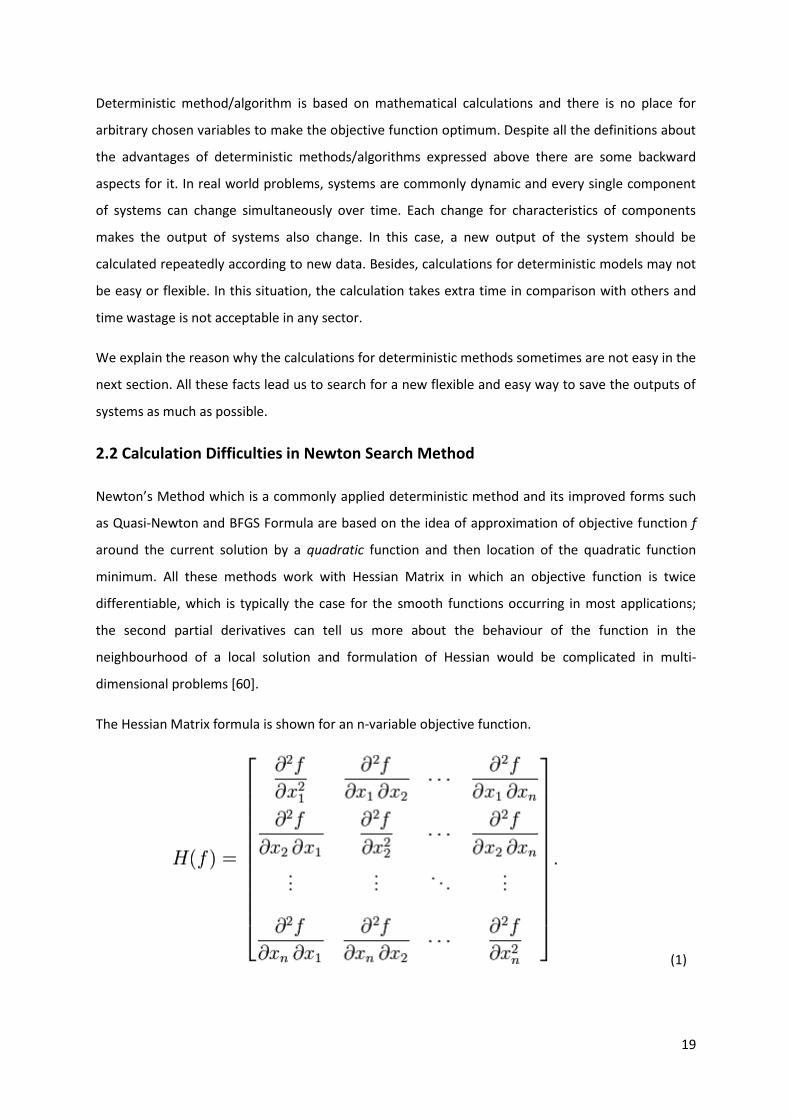
2.2 Calculation Difficulties in Newton Search Method

Newton’s Method which is a commonly applied deterministic method and its improved forms such

as Quasi-Newton and BFGS Formula are based on the idea of approximation of objective function f

around the current solution by a quadratic function and then location of the quadratic function

minimum. All these methods work with Hessian Matrix in which an objective function is twice

differentiable, which is typically the case for the smooth functions occurring in most applications;

the second partial derivatives can tell us more about the behaviour of the function in the

neighbourhood of a local solution and formulation of Hessian would be complicated in multi-

dimensional problems [60].

The Hessian Matrix formula is shown for an n-variable objective function.

(1)

20

Even searching via deterministic methods has some advantages such as convergence speed, starting

with a closer point to optimum and constant search results; there are also some backward aspects to

applying them. Basically, there are some types of problem such as Non-deterministic Polynomial-

time (NP) not eligible for applying to deterministic methods based on Newton’s Method Search and

its improved forms.

Even though deterministic methods are very useful especially for analytical problems, basic

calculations for deterministic methods may have a high cost because of time wastage and

calculation cost. Besides, there is a big risk of falling with the local optimum and hill climbing while

searching for a global optimum. This means that searches for the global optimum may be misled and

so, researchers may not benefit from the global optimum which also means extra cost.

In case researchers face the disadvantages of applying deterministic methods, another way should

be sought to beat the hill climbing and to find the global optimum or approximate it better than

deterministic methods.

In the next section and further, we will describe and apply heuristic methods as an alternative way

to searching by deterministic methods.

2.3 Heuristic Optimisation

In recent decades, tackled optimisation problems have been getting more difficult or impossible to

solve by applying the usual optimisation algorithms such as deterministic methods, which have been

replaced by several heuristic methods and tools [11].

Heuristic algorithms are criteria and computational methods which decide on an efficient way

among alternative methods to reach any goal or solution. These algorithms’ approximations to the

global optimum are not provable. Heuristic algorithms have approximation attributes but do not

guarantee the exact solution unlike deterministic algorithms that guarantee a solution near to the

global optimum. Basically, heuristic algorithms are inspired by nature’s behaviour such as bee and

ant colonies because: creatures’ mechanisms are too complicated and cannot be explained by

mathematical formulations, so this condition fits problems which are not eligible to be solved by

mathematical based methods. There are many reasons for applying heuristic algorithms.

Firstly, there may not be an available method among traditional algorithms to find an exact solution

for the tackled optimisation problem such as NP-hard. In this case, researchers should find a new

suitable method for this kind of problem.

21

Secondly, heuristic algorithms can be more helpful because they are not based on complicated

formulas unlike deterministic algorithms. Besides, heuristic algorithms are suitable to apply as a part

of different algorithms to improve their efficiency for searching for an exact solution; however, this

advantage is not easy to implement on deterministic algorithms.

In addition, mathematical formulation-based deterministic algorithms usually disregard the most

difficult aspects (which aim and boundaries, which alternatives can be tested, how to collect

problem data) of real world problems. If the tackled deterministic algorithm uses incorrect

parameters it may find a solution much worse than a heuristic approach. Heuristic algorithms can

tolerate incorrect data because they are not based on mathematical formulations; therefore,

heuristic methods are more flexible than deterministic methods.

Despite all these advantages of heuristic algorithms, there are some criteria to determine them as an

applied method instead of a deterministic method because optimisation problem characteristics

determine which method is useful or not. Criteria about evaluation of a heuristic method are aligned

as:

Obtained solution quality and convergence time are really important criteria for making

decisions about the efficiency of any heuristic algorithm. Therefore, a qualified algorithm should

have changeable parameter sets which are able to be compared easily according to their

calculation cost and obtained solution quality attributes. In other words, the connection

between obtained solution quality and convergence time should be considered.

The applied algorithm should be applicable commonly and its components should be clear to

understand the system easily. In this condition, even though there is little information about

problem characteristics, the attributes mentioned above allow the algorithm to be applied

easily in new areas.

Heuristic algorithms involve flexible characteristics because they have to provide instant

changes for objective function and boundaries. Thus, heuristic algorithms can answer to all

conditions and problems

Heuristic algorithms should be capable of re-generating acceptable high quality solutions, in

other words robust, which are not dependent on the initial solution swarm. In this way, they

can tolerate incorrect initial data or swarm.

It should be easier to analyze the applied heuristic algorithm due to its flexibility and obtained

solution quality compared with complicated algorithms which may not be eligible for

considering their mentioned attributes.

22

Various algorithm users expect more attractive interface or easier usage from algorithm

designers. A useful algorithm should be capable of providing some visual tools such as graphics,

figures which make algorithms more understandable. This fact is very important to support the

interaction between machines/computers and users.

Heuristic algorithms are based on greedy neighbourhood search methods to improve initial solutions

(swarm) step by step to reach the global optimum or approximate it [29]. Some heuristic-

neighbourhood (local) search algorithms generate the local optimum based on initial solutions and

this situation is common for iterative improvable algorithms. In some cases, the local optima could

be far from the global optima and cannot approximate them. Besides, in the most discrete

optimisation problems, necessary information may not be available to determine the useful initial

solution heap. In order to eliminate some disadvantages of heuristic-local search methods, some

options are aligned and providing clearness and generality;

The heuristic-local search could be started with multiple initial solutions and apply the same

number of iterations for them; however, randomly distributed different solutions may have

high cost and this technique does not guarantee optimum solutions because of possible

different aims of initial solutions.

If researchers focus on defining a complex neighbourhood function rather than multiple initial

solutions, they can probably obtain better solutions regenerated from previous ones.

Researchers can use complex learning strategies to get information about running algorithms

and then this information can be used to define the penalized solutions or districts in the

feasible area. In this way, they can avoid processing the same solution repeatedly.

It is acceptable that, if a movement from a solution to another takes the algorithm out from

local optima and avoids falling hill climbing, this movement should be applied even if it is not

beneficial because the primary purpose of local search methods is approximating the global

optima as much as possible [12].

According to all information about advantages and disadvantages of heuristic algorithms with their

insufficient aspects, researchers need to choose or improve methods and tools that should be

flexible to tolerate various conditions.

In recent years, researchers have been trying to combine algorithms among these new tools with

their knowledge elements to improve search quality and apply the hybrid algorithms’ challenging

problems. In this dissertation, we will also use the same way to obtain better solutions. Hybrid

algorithms are able to give two advantages to researchers. Developed hybrid algorithms may

23

decrease the run time by developing calculation techniques or decreasing the number of iterations.

On the other hand, the hybridization process can make an algorithm more robust and flexible. In this

way, developed algorithm can tolerate more noise and/or missing data and changing conditions [11].

In recent years, most optimisation problem researchers are trying to develop new algorithms and

apply them in case studies and real world optimisation problems. Kovacevic et al. [13] developed a

new meta-heuristic method and applied it to determine optimal values of machining parameters

traditionally performed by algorithms based on mathematical models and exhaustive iterative

search. The main reason for the meta-heuristic model in [13] is that, meta-heuristic methods are

capable of handling various optimisation problems and obtaining high quality solutions by running

less iteration, in other words less computational time. Their motivation for the development of the

software prototype was obtaining sufficient solutions from the meta-heuristic algorithm. Li et al. [14]

applied a particle swarm optimisation approach -a branch of heuristics- and developed an

adjustment strategy for weighted circle packing problems which is a kind of important combination

optimisation problem and has an NP-hard characteristic. The purpose of this [14] study is to obtain a

better layout scheme for larger circles and show that the proposed method is superior to the

existing algorithms in performance. Liu and Xing [15] constructed a special heuristic method for the

double layer optimisation problem proposed to answer rapid developing logistic systems via

advanced information technologies by reforming the current system. In [15], experimental results

correctly proposed methods and heuristic feasibility. Kaveh and Khyatazadat [16] developed a new

branch of heuristic methods called ray optimisation. The main idea of this new optimisation method

is based on Snell’s law about light travel and its refraction— in other words its direction changes.

The purpose of this [16] development is to increase the effectiveness of optimisation elements in

search phase and converge phase. Min et al. [17] searched for efficient algorithms to find the best

orientation between two randomly deployed antennas -capable of determining the best orientation

to receive the strongest wireless signal- under the effect of various wireless interferences. In [17],

four different heuristic optimisation methods with some modification are presented as candidates

and are also described with test cases and real world experiments to determine which algorithm is

suitable to apply.

On the other hand, heuristic algorithms involve a few disadvantages beside their advantages. Firstly,

heuristic methods usually take longer convergence time in comparison with deterministic methods.

In case we consider mathematical based problems, deterministic methods such as Quasi-Newton

method, golden section search, and quadratic fit search would be more useful due to shorter

convergence time than heuristic methods spend. Besides, deterministic methods are able to reach

24

exact solutions for deterministic problems. However, if heuristic algorithms are applied on

deterministic methods, they may not reach exact solutions.

In this study, one heuristic method is tackled and modified with another one to obtain a better

solution for a specific NP-hard real world problem. Before implementation of these algorithms,

braches of heuristic optimisations are described briefly.

2.3.1 Evolutionary Computation

In the last decades, many researchers have been interested in evolutionary based algorithms and

the number of studies about this field has increased significantly and all these studies are considered

subfields of evolutionary computation [18]. This algorithm simulates the hypothetical population

based natural evolution optimisation process on a computer resulting in stochastic optimisation

methods. This way can obtain better solutions than traditional methods in difficult real world

optimisation problems [11].

Evolutionary computation mainly consists of evolutionary programming, evolution strategies,

genetic algorithms, and differential evolution. Besides, many hybrid algorithms replicate some

evolutionary algorithm attributes. Generally, all these algorithms require five major elements;

genetic representation of solutions, generator methods for initial solutions population, fitness

evaluation function, and operators differentiating the genetic structure and values of control

parameters. Evolutionary algorithms improve all the solution population instead of one single

solution [18]. In this way, these algorithms are able to increase their effectiveness and convergence

speed while searching for global optimum/optima.

2.3.1.1 Genetic Algorithm

Genetic algorithm is based on generating a new set of solution populations from the current one

inspired by the conjecture of natural selection and genetics to improve the fitness of solutions. This

process continues until the stopping criteria are satisfied or the number of iterations reaches its

limitation. Genetic algorithms involve three elements to obtain sufficient results from a search:

reproduction, crossover, and mutation [19].

The reproduction operator works with the elimination of candidate solutions according to their

quality inspired by natural selection. The crossover operator provides generating hybrid structures

25

to increase the number of outputs. The mutation operator is a basic structure of a genetic algorithm

inspired by natural genetic mutation by checking all bits of solutions and reversing them according to

their mutation rate. These operators generate more candidate solutions to increase the number of

options [18].

Genetic algorithm is different from other search methods due to its specialized attributes: multipath

search to reduce the possibility of being trapped in local optimum area, coding parameters

themselves to make genetic operators more efficient by minimizing step computation, evaluating

only objective function (in other words, fitness) to guide the search, no requirement for computation

of derivatives or other auxiliary functions to make this algorithm easy to apply, and searching space

with high probability of obtaining improved solutions [11]. These attributes make the genetic

algorithm applicable to all kinds of problems such as discrete, continuous, and non-differentiable

problems [19].

Genetic algorithm can be applied to bin packing problems. Goncalves and Resende [20] developed a

kind of genetic algorithm named novel biased random key (BRKGA) for 2-D and 3-D bin packing

problems, which can be more complex than 1-D bin packing problems according to their shape

complexity. They improved the solution quality significantly with a modification on the placement

algorithm. In this way, they proved that an applied placement algorithm can outperform all other

ones.

2.3.1.2 Evolution Strategies and Evolutionary Programming

Evolution strategies rely on the mutation process as a search operator and evolving the strings from

a population size of one. Evolution strategies are similar to the genetic algorithm in a few aspects.

The major similarity between them is using selection process to obtain the best individuals from

potential solutions. On the other hand, three main differences between genetic algorithm and

evolution strategies can be expressed as: type of operated structures, basic operators they rely on

and the link between an individual and its offspring they maintain [11].

Evolutionary programming (EP) is a stochastic optimisation method developed by Lawrence J, Fogel

and his co-workers in the 1960s. Evolutionary programming has also many similarities with the

genetic algorithm like evolution strategies. However, this technique does not imitate nature like the

genetic algorithm emulates a specific genetic operator; EP emphasizes the behavioural link between

individuals and their off-spring like evolutionary strategies do. In this way, EP does not involve

mutation or crossover operations together [21]. In fact, evolutionary programming and evolutionary

strategies are similar but developed by applying different approaches [11]. Evolutionary

26

programming was thought as an applicable method just for evolving finite states for prediction tasks

for a long time. After a while, it appeared that this method is also eligible to optimise the continuous

function with real valued vector representation [21].

2.3.1.3 Differential Evolution

Differential evolution is the most powerful population based optimisation method with its simplicity

[22]. Mutation operation is also processed by the DE algorithm like other sophisticated evolutionary

algorithms. However, the main difference between them is the type of applied method for the

mutation process. The method the DE algorithm applies is using differences of random pairs of

objective vectors [11]. Random candidates (pairs) are generated by different techniques and if new

generated candidates beat existing ones, new pairs replace them and in this way, the DE algorithm

acquires a more efficient search technique to find the global optimum [22].

The differential evolution algorithm is a direct search method based on a stochastic process and is

considered as accurate, reasonably fast and robust. It is easy to apply for minimization processes in

real world problems and multimodal objective functions. Mutation operation process in the DE

algorithm uses arithmetical combinations of individuals whereas the genetic algorithm uses the

method of perturbing genes in individuals with small probability. Besides, DE algorithms do not use

binary representation unlike genetic algorithms for searching. Their search works with floating point

representation. All these main characteristics make this algorithm a competitive alternative and

attractive especially for engineering optimisers [11].

2.3.2 Swarm Intelligence

Researchers have recently been interested in swarm intelligence by imitating animals’ foraging or

path searching behaviours like in Particle Swarm Optimisation, Ant Colony Optimisation and Bee

Colony Optimisation.

2.3.2.1 Particle Swarm Optimisation

Particle swarm optimisation (PSO) is based on simulating a swarm of birds foraging, initially

introduced by Kennedy and Eberhart in 1995 [23]. The PSO algorithm is initialized with random

solutions (swarm) like other sophisticated evolutionary computation algorithms [11]. Swarm and

particles correspond to the population and individuals in other evolutionary computation techniques

27

respectively. Particles of a swarm move in multi dimensional space and each particle’s position in

this space is adjusted according to their and their neighbours’ performance [24].

The PSO algorithm is similar to other population based algorithms in many aspects. PSO is also useful

for optimising a variety of difficult problems. Besides, it is possible that the PSO algorithm can show

higher convergence performance on some problems. The PSO algorithm requires a few parameters

to adjust and this attribute makes the algorithm more compatible with implementations. On the

other hand, PSO can fall into local minima easily [24].

Liu et al [20] improved on a formulation for 2-D bin packing problems with multiple constraints

abbreviated as (MOBPP-2D). They proposed and applied a multiobjective evolutionary particle

swarm optimisation algorithm (MOEPSO) to solve MOBBP-2D and performed the formulation with

MOEPSO on various examples to make a comparison between the developed formulation embedded

particle swarm algorithm and other optimisation methods introduced in the paper. This comparison

illustrates the effectiveness and efficiency of MOEPSO in solving multiobjective bin packing

problems.

2.3.2.2 Ant Colony Search Algorithm

Basically, an ant colony optimisation algorithm (ACO) imitates the foraging activities of an ant colony

based on a random stochastic population. The ACO algorithm is a considerable method for

optimising combinatorial optimisation problems and real world applications. Ant colonies have an

interesting behaviour in that they can find the shortest path to reach a food source from their nest

while foraging. In order to find or change the path the colony uses, each ant deposits on the ground

a chemical substance called a pheromone. Marked paths by strong pheromone concentration allow

ants to choose their path to find the nest or food sources in quasi random fashion with probability.

Basically, the ACO algorithm applies two procedures: specifying the way of solution construction

performed by ants for the problems and updating the pheromone trail [25].

Fuellerer et al [26] considered a 2-D vehicle loading as part of the routing problem. Probable

solutions to this problem involving routing success depend on loading success and should satisfy the

demand of the customers. They applied different heuristic methods to obtain an optimum solution

for loading part and applied ant colony algorithm (ACO) for overall optimisation. Determinative

factors of this problem are size of the items and their rotation frequency. Gathering information

about these factors allow us to make low cost decisions in the transportation sector. Fuellerer et al’s

investigation about the combination of different heuristic methods with ACO was insufficient;

however, in [26] their approach obtained sufficient results for this combination.

28

2.3.2.3 Artificial Bee Colony (ABC) Algorithm

The bee colony algorithm is one of the most recent population based metaheuristic search

algorithms first systematically developed by Karaboga [29] and Pham et al [30] in 2005.

Independently however these two are slightly different. Basically, they use the same techniques to

generate initial swarm explained in the next chapters; however, they use different elimination

technique for bees.

As mentioned in previous sections, scientists are inspired by natural occurrences and they

investigate the behaviours of creatures to adapt these behaviours to the artificial systems. The main

reason for simulating nature rather than applying mathematical calculations is that, creatures can

overcome the problems they face every moment with guidance of their instincts. In this section, a

bee swarm behaviour based algorithm is introduced step by step.

Basically, the Artificial Bee Colony (ABC) algorithm applies two main search methods as a

combination, neighbourhood search and random search, to obtain optimum solutions for various

problems. The ABC algorithm is inspired by food searching techniques and shares information about

sources between bees in a honey bee swarm. Moreover, the ABC algorithm includes a hierarchical

system and in this way, the bee swarm assigns bees and divides them according to their mission in

the swarm. Definitions for bees’ missions can change throughout the food search. Even though the

ABC algorithm is a recently developed algorithm, it is considered very promising by many

researchers with sufficient results from experiments in a variety of optimisation problems. The ABC

algorithm is also eligible for modification or as part of a combination with other algorithms as the

main characteristic of heuristics. There are many studies about the ABC algorithm.

Karaboga inventor of the ABC algorithm has also published papers about this algorithm and

improved his idea over time. Karaboga and Ozturk [31] applied the ABC algorithm for data clustering,

used in many disciplines and applications as an important tool for identifying objects based on the

values of their attributes, on benchmark problems and compared with the Particle Swarm

Optimisation (PSO) algorithm and nine other classification techniques [31]. On average, the ABC

algorithm achieved better optimum solutions as a cluster than other algorithms for a variety of

tackled datasets in [31]. Akay and Karaboga [32] applied a modified ABC algorithm for real

parameter optimisation to increase the efficiency of the algorithm and the results of this modified

algorithm and three other algorithms were compared. In [32], the standard ABC algorithm and

modified ABC algorithm present different characteristics with different kinds of problems. In this

study, ABC algorithm techniques developed by Karaboga are applied on the problem we tackle as a

29

base because ABC algorithm involves a swarm based search which is based on starting to search

from multiple points in feasible area which means that ABC algorithm is capable of reducing

convergence (to global optimum) time. Besides, studies about ABC algorithm [30], [31], [32] express

the other valuable aspects of this algorithm and all these factors lead us to focus on this algorithm.

Pham et al [30] developed the bees algorithm as mentioned above and they demonstrated the

efficiency of the newly developed algorithm on different functions. The results of the bees algorithm

are sufficient and very promising for further studies. There is another study that shows the efficiency

of the bees algorithm by applying it on a real world problem, also published by D.T. Pham as a

participant in [33]. Xu et al [33] applied a binary bees algorithm (BBA), which is different from a

standard bees algorithm, to solve a multiobjective multiconstraint combinatorial optimisation

problem. They demonstrated the treatment of this algorithm by explaining the change of

parameters.

Many other researchers have also benefited from the bees algorithm. Dereli and Das [34] improved

a hybrid bees algorithm for solving container loading problems. The aim in this problem is loading a

set of boxes into containers which are discrete variables to be worked. They explain the necessity of

applying a hybridized algorithm for the container loading problem and comparing the mentioned

hybrid algorithm with other algorithms known in literature. The study demonstrates that, according

to the results, the hybridized bees algorithm obtains promising solutions and the standard bees

algorithm is also very stimulating with its techniques for further studies in optimisation. Kang et al

[35] also proposed a hybridized algorithm for searching for numerical global optimum and this

algorithm was applied on a comprehensive set of benchmark functions. In [35], the results show that

a new improved algorithm is reliable in most cases and is strongly competitive. Ozbakir et al [36],

developed the standard bees algorithm (BA) to apply a generalized assignment problem, which is an

NP-hard problem, and compared this algorithm with several algorithms from the literature. In order

to investigate the performance of the proposed algorithm further, they applied it on a complex

integer optimisation problem. According to the results and comparisons between several algorithms,

they found the bees algorithm and proposed algorithm promising and these algorithms can be

improved further. Gao and Liu [37] also improved the standard artificial bee colony (ABC) algorithm

by using a new parameter with two improved solution search equations and then applied the new

algorithm on benchmark functions and compared it with different algorithms according to their

convergence performance for numerical global optimum. The results of the improved ABC algorithm

show sufficient performance in all criteria. They also strongly recommend other researchers to carry

out further studies about the bees colony algorithm. Xiang and An [38] improved the standard

30

artificial bee colony to accelerate the convergence speed. Besides, they made a change in the scout

bee phase to avoid being trapped in local minima. In [38], several benchmark functions are tested by

applying the improved algorithm and two other ABC based algorithms for a comparison between the

mentioned algorithms. According to test results, the improved algorithm can be considered as a very

efficient and robust optimisation algorithm. Szeto et al [39] proposed an enhanced version of the

standard ABC algorithm to improve the solution quality. They applied the standard and enhanced

ABC algorithm for one of the real world problems, which is the capacitated vehicle routing problem

by using two sets of standard benchmark instances. In comparison, the enhanced algorithm

outperformed the standard algorithm.

All these papers about the bees colony or artificial bee colony algorithm show that there is a wide

area for possible and promising improvements for the standard ABC algorithm which is also eligible

for modification by using different equations, formulations or parameters. It is also possible that

other heuristic/deterministic algorithms with entire structure or a minor part can be merged with

the ABC algorithm easily. The main objective of improvements or hybridizations on the ABC

algorithm is obtaining better solutions and making the algorithm more robust. There are not only

advantages to the ABC algorithm, it has also some disadvantages. Even though convergence speed

of the ABC algorithm can be sufficient in most studies, the robustness of the ABC algorithm needs to

be improved because a robust algorithm is not affected by parameter changes or misleading starting

points and it can obtain approximately same results in this circumstance.

All creatures use different techniques for foraging repeatedly in a sequence with guidance of their

instinct. The ABC algorithm mimics the bee behaviours in swarm and nature as mentioned above

and uses the same collective intelligence of the forager honey bee. There are three main

components of the ABC algorithm: food sources, employed foragers and unemployed foragers.

Besides, forager bees use two main behaviours, recruitment for a nectar source and abandonment

of a nectar source [29].

Food Sources: The source eligible or not for foraging visited by honey bees can be chosen due to its

overall quality. There are many factors to measure the food source quality such as the distance

between nest and source, food level, and nectar quality [29]. In the ABC algorithm, every single food

source represents a possible solution in a feasible area and the overall food quality represents the

fitness of possible solutions as well [40].

Employed Foragers: Forager bees are sent to food sources explored and determined by scout bees

to exploit the nectar until they reach their capacity. Forager bees are not only carrying the nectar,

31

they also transfer information about food sources to share with other unemployed bees. The

information about food sources is shared with certain probability. In this way, scout bees can

determine the best food source in the environment they investigate and onlooker bees can find the

food source easily.

Unemployed Foragers: Unemployed bees consist of two types, onlooker bees and scout bees. Scout

bees search the environment surrounding the nest for new sources or update information about

existing sources. Onlooker bees wait in the nest to gather information about food sources from

employed bees or scout bees. In a hive, the percentage of scout bees is between 5-10% [29].

Collective intelligence of bee swarms is based on the information exchange between honey bees.

Every single bee shares the information they have on a kind of stage with others. In this way, they

can do their job with minimal failure. The most important occurrence while they exchange

information is a kind of dancing on a stage in the hive. This dance is called a waggle dance.

Fig. 3: The Waggle Dance Performed by Honey Bees [58]

Austrian ethologist Karl von Frisch was one of the first people to translate the meaning of the waggle

dance. If the food source is less than 50 metres away from the hive, the bee performs a round dance

otherwise it performs a waggle dance. In addition, honey bees perform a waggle dance with

different movements and speed. In this way, they can communicate among the swarm and share

information about food sources.

The waggle dance consists of five components [41]:

Dance tempo (slower or faster)

32

The duration of the dance (longer duration for better food source)

Angle between vertical and waggle run means angle between sun and food source

Short stop in which the dancer shares the sample of food source with their audience

Other bees follow the dancer (audience) to gather information from the dancer.

The audience of the waggle dance determines the most profitable food source according to dance

figures and then they divide the food source environment. There is a foraging cycle in the collective

intelligence. This cycle involves four types of characteristics to provide the necessary information to

other bees:

Positive Feedback: If the highest nectar amount of the food sources in an environment increases,

the number of visitors (onlooker bees) increases as well.

Negative Feedback: If the nectar amount of a food source is exploited completely or has poor

quality, it is not found sufficient and onlooker bees stop to visit this source.

Fluctuation: Random search process for exploring the promising food sources is carried out by

scout bees

Multiple interactions: As mentioned above, scout bees and forager bees share their information

about food sources with onlooker bees on the dance area [29].

Fig. 4: The behaviour of honey bee foraging for nectar [29]

Abbreviations in Fig. 4 represent the following: Scout bees (S), newly recruited (onlooker) bees (R),

uncommitted follower bees after abandoning the food source (UF), returning forager bees after

33

performing a waggle dance for an audience (EF1), and returning forager bees without performing a

waggle dance (EF2) [40].

2.3.2.3.1 Formulation of ABC Algorithm

In the ABC algorithm, the number of onlooker bees or employed bees equals the number of

solutions in the populations. In fact, there is no difference between onlooker bees or employed bees

in the ABC algorithm because the initial population cannot be changed; however, in nature it can be

changed due to the needs of the swarm.

As the first step, the initial population is generated randomly for solutions in a feasible area. In the

ABC algorithm, initial solutions represent the food source positions in an environment. Each solution

xi (i = 1, 2, … SN) is a K-dimensional vector where K is the number of characteristics, in other words

the parameters of the investigated solution in optimisation, and SN is the size of the initial

population. Parameters for each solution can be represented as k (k = 1, 2, …, n) and the following

definition might be used for initialization to generate the solution vector:

(2)

where; and are the lower bound and upper bound of the parameter , respectively.

After generating the initial population with their parameters, bees can separate and start the second

phase. It is important that after generation of food sources, every single bee goes to only one food

source in the employed bees phase.

In the employed bees phase, all bee swarms separate to the source field homogeneously and every

single food source represents one honey bee. The employed bees search for new possible food

sources ( ) and this process is a kind of random neighbourhood search; so, they move from the

memorized source ( ) to the neighbour source to investigate the food quality and food level.

Neighbour solutions around the initial solutions in a cycle have different fitness value and the honey

bees evaluate them in this phase. The following equation defines the neighbourhood function to

generate the neighbour solutions;

(3)

Where is randomly selected food sources, i is a randomly chosen parameter index and is a

random number positive or negative in range. After generating the neighbour food sources, the bees

evaluate the sources and they make a greedy selection according to fitness values of neighbour food

sources. The fitness value of the solution ( ), can be calculated with the following equation;

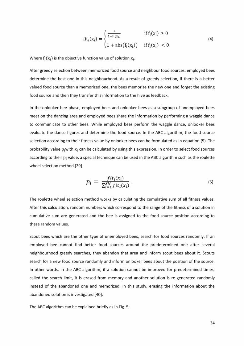
34

(4)

Where is the objective function value of solution .

After greedy selection between memorized food source and neighbour food sources, employed bees

determine the best one in this neighbourhood. As a result of greedy selection, if there is a better

valued food source than a memorized one, the bees memorize the new one and forget the existing

food source and then they transfer this information to the hive as feedback.

In the onlooker bee phase, employed bees and onlooker bees as a subgroup of unemployed bees

meet on the dancing area and employed bees share the information by performing a waggle dance

to communicate to other bees. While employed bees perform the waggle dance, onlooker bees

evaluate the dance figures and determine the food source. In the ABC algorithm, the food source

selection according to their fitness value by onlooker bees can be formulated as in equation (5). The

probability value with can be calculated by using this expression. In order to select food sources

according to their value, a special technique can be used in the ABC algorithm such as the roulette

wheel selection method [29].

. (5)

The roulette wheel selection method works by calculating the cumulative sum of all fitness values.

After this calculation, random numbers which correspond to the range of the fitness of a solution in

cumulative sum are generated and the bee is assigned to the food source position according to

these random values.

Scout bees which are the other type of unemployed bees, search for food sources randomly. If an

employed bee cannot find better food sources around the predetermined one after several

neighbourhood greedy searches, they abandon that area and inform scout bees about it. Scouts

search for a new food source randomly and inform onlooker bees about the position of the source.

In other words, in the ABC algorithm, if a solution cannot be improved for predetermined times,

called the search limit, it is erased from memory and another solution is re-generated randomly

instead of the abandoned one and memorized. In this study, erasing the information about the

abandoned solution is investigated [40].

The ABC algorithm can be explained briefly as in Fig. 5;

35

In addition, an ABC algorithm flowchart is demonstrated in Fig. 6. The ABC algorithm has some

disadvantages beside its advantages. For instance, many researchers have proposed several models

to enhance the ABC algorithm because of its weak robustness (explained in page 30) characteristic

especially. In this study, we will try to overcome weak robustness characteristic of ABC algorithm

with some additional techniques explained in the next chapter.

1: Initialize the population of solutions xi, (i = 1, …, SN)

2: Evaluate the population

3: cycle = 1

4: repeat

5: Produce new solutions vi for the employed bees from existing solutions by

using (3) and evaluate them

6: Apply the greedy selection process for the employed bees

7: Reset the counter if solution is improved otherwise add one to counter

8: Calculate the probability values Pi for the solution xi by (5)

9: Produce an amount of new solutions vi for the onlooker bees from the

solutions xi depending on Pi and evaluate them

10: Apply the greedy selection process for the onlooker bees

11: Reset the counter if solution is improved otherwise add one to counter

12: Check the counter for solutions if they exceed the limit or not and

determine the abandoned solution for the scout, if exists, and replace it

with a new randomly produced solution xi by formulation (2)

13: Memorize the best solution achieved in one cycle

14: cycle = cycle + 1

15: until predetermined number of cycle [40].

Fig. 5: Pseudo Code for Classic ABC Algorithm

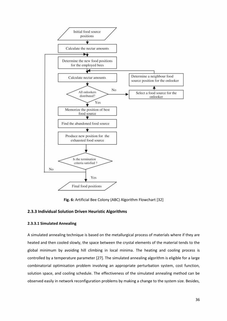
36

Fig. 6: Artificial Bee Colony (ABC) Algorithm Flowchart [32]

2.3.3 Individual Solution Driven Heuristic Algorithms

2.3.3.1 Simulated Annealing

A simulated annealing technique is based on the metallurgical process of materials where if they are

heated and then cooled slowly, the space between the crystal elements of the material tends to the

global minimum by avoiding hill climbing in local minima. The heating and cooling process is

controlled by a temperature parameter [27]. The simulated annealing algorithm is eligible for a large

combinatorial optimisation problem involving an appropriate perturbation system, cost function,

solution space, and cooling schedule. The effectiveness of the simulated annealing method can be

observed easily in network reconfiguration problems by making a change to the system size. Besides,

37

the cost function is helpful for the simulated annealing algorithm to escape more easily from local

minima and to perform rapid convergence [11].

Rao and Iyengar [28] proposed an efficient version of the simulated annealing method compared

with well-known heuristic algorithms according to implementation results of a variant of the bin

packing problem. They obtain sufficient and high quality solutions by applying the developed

algorithm.

2.3.3.2 Tabu Search Method

Tabu search (TS) algorithm is metaheuristic and was developed by F. Glover. The purpose of the TS

algorithm is to increase the performance of the neighbourhood search function applied on many

heuristic algorithms by improving the search techniques. The TS algorithm provides a further search

beyond the existing best solution in a feasible area by using the best move in the previous cycle to

generate a new solution. In other words, the TS algorithm memorizes the best move in iteration

[42].

As the TS algorithm proposes a more efficient neighbourhood search for general heuristic

optimisation problems, many researchers use this method to enhance the algorithm applied on

tackled problems. In other words, the TS algorithm is a promising method for further studies.

Mashinchi et al [43] proposed a new algorithm based on the Tabu Search and Nelder Mead (NM)

search strategy with an additional phase for increasing the robustness of the proposed method.

They applied the new developed algorithm on a real world problem which is global continuous

optimisation problems. They applied the TS method to enlarge the search field and decrease the

possibility of being trapped in local minima. In this way, convergence speed of the proposed hybrid

algorithm can be accelerated and this speciality can make the mentioned algorithm competitive in

comparison with other algorithms. The proposed algorithm has two main advantages; it is applicable

for any global continuous optimisation problem without considering any constraints and it shows

better performance for small and medium input domains in the given multimodal functions. Ji and

Tang [44] proposed a new tabu search based on applying a memory system for solving the multiple

minima problem of continuous functions. The proposed method is based on two convergence

theorems introduced by them. Numerical results show that proposed algorithm is efficient, robust

and suitable for implementations. Ahonen et al [45] applied the tabu search method on several

corridor allocation problem instances with different datasets generated randomly or taken from

literature to compare with the simulated annealing algorithm. The results show that the simulated

annealing algorithm outperforms the tabu search method. This paper [45] shows that the

38

effectiveness of an algorithm depends on problem type and characteristics of datasets. The

scheduling problems have been challenging in the last few decades and one of them is tackled by

Belle et al [46] who applied a tabu search approach for it. The purpose of this [46] paper is

minimizing the total travel time and the tardiness in the truck scheduling problem. Calculating the

optimum solutions with a mixed integer programming solver, using a mathematical model, takes a

lot of computation time. They improved the results calculated by integer programming and

shortened the computation time by applying the tabu search approach and stated that the proposed

method is promising for future studies. Jia et al [47] developed a new tabu search working with

mutation and mixed local search operators to overcome the weaknesses of the standard tabu

search. In comparison, the proposed tabu search is much more sufficient than other algorithms

according to vehicle route problem implementation results because it is more applicable on whether

the size of the problem is big or small and the convergence speed is fast with efficient calculation.

Tao and Wang [48] proposed a new tabu search approach for the 3-D loading sub-problem of the

vehicle routing problem (3L-CVRP), which combines the routing of a fleet of vehicles and the loading

of 3-D shaped goods. The purpose of this [48] paper is minimizing the total travel distance with

minimizing the wastage. According to experiment results, the proposed approach shows higher

performance compared with other algorithms in terms of both solution quality and efficiency.

The main idea of the TS algorithm is using memory to check the search history. Throughout the

search, some bad moves can be memorized in the short term and added to a limited list called a

Short Term Tabu List (STTL). The purpose of the STTL is to avoid being trapped in local minima and it

works with a first in first out system. Besides, if a good move is found in a cycle it is added to long

term memory called a Long Term Tabu List (LTTL). LTTL shows that the field containing a memorized

solution has been investigated before. These two lists keep the memorized moves for a

predetermined number of cycles and then they are erased.

The TS algorithm is a tool for escaping the local minimum and overcoming the hill climbing; however,

the next point can be worse than the current one in a local minimum. In this way, the TS algorithm is

protected from being trapped in the local minimum [43].

The TS algorithm generates a finite number of neighbours around the current solution and can

consider these neighbours for the next iterations. Period of a move in the tabu list is a basic control

parameter in the TS algorithm. Secondary control parameter is the size of the tabu list which

denotes the determined maximum number of moves, in other words capacity, in the tabu list. The

tabu list logic uses the first in first out (FIFO) algorithm to enroll the move into the list or erase it.

Chosen move from neighbourhood search is enrolled to the tabu list for a period and at the end of

39

this period the move is erased from the list. If the tabu list is full, the first added move is erased and

the chosen move enrolled instead of it. The basic Tabu Search algorithm based on STTL is illustrated

in Fig. 7.

Several heuristic algorithms explained above have been applied in the last few decades to overcome

real world problems which are difficult to solve by applying classic methods. Even though these

algorithms are based on trial and error logic, they obtain promising and competitive results in real

world problems.

In the next section, one of the real world problems, found interesting by researchers in recent years,

is defined and detailed.

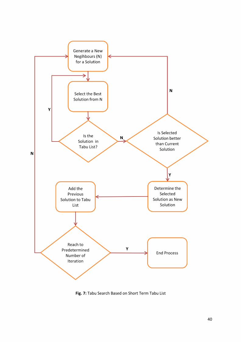
40

Fig. 7: Tabu Search Based on Short Term Tabu List

41

2.4 Bin Packing Problems

Engineers always have to overcome many real world problems and they may be unable to reach

sufficient solutions to these problems in proper time. Because of this weakness of workers or

engineers, scientific backgrounds provide them with suitable approaches for tackled problems. On

the other hand, operators may also explore some approaches for their problems by using trial and

error techniques. In both cases, they have to find an acceptable way to reach solutions.

One of these real world problems is called the Bin Packing Problem which involves basically loading a

finite number of capacitated alike repositories with various dimensional shaped goods. The bin

packing problem is a combinatorial NP-hard problem. Finding the optimum solution is known to be

exponentially difficult. The object of bin packing problems is minimizing the number of bins and

wastage.

Cutting stock problems are also a version of bin packing problems and the main objective is that,

when the bin is stated as 1, this problem maximizes the number of packed items. Volume and value

specialities are also determinative characteristics in cutting stock problems.

Many heuristic approaches have been developed and proposed including advantages and

disadvantages to solve the bin packing problems. The bin packing problem can be categorized by

dimensional characteristics and the problem definition is based on the relation between items and

bins.

If all items and bins have two similar superficies, they can be categorized as a one dimensional (1D)

bin packing problems set. If all of them have similar superficies, they can be categorized as a two

dimensional (2D) bin packing problems set. If all items and bins have totally different superficies,

they can be categorized as a three dimensional (3D) bin packing problems set.

Packing approaches may change due to the dimensional relation of bin packing problems sets. In this

study, a set of the 1D bin packing problem is considered with classic algorithms and another

heuristic approach.

Bin packing problem approaches involve the information about items’ supply system. If the packing

operator works with an offline supply system, the operator has all the information about items to

allocate them into bins by categorizing due to their shape. On the other hand, if the packing

operator works with an online supply system, the operator may not allocate the arrival items into

bins as in the offline supply system. In this case, the supply system speciality is also determinative

for bin packing problem approaches.

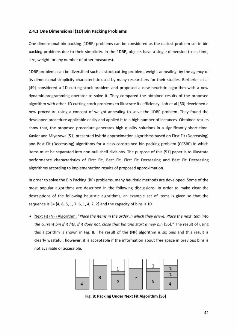
42

2.4.1 One Dimensional (1D) Bin Packing Problems

One dimensional bin packing (1DBP) problems can be considered as the easiest problem set in bin

packing problems due to their simplicity. In the 1DBP, objects have a single dimension (cost, time,

size, weight, or any number of other measures).

1DBP problems can be diversified such as stock cutting problem, weight annealing. by the agency of

its dimensional simplicity characteristic used by many researchers for their studies. Berberler et al

[49] considered a 1D cutting stock problem and proposed a new heuristic algorithm with a new

dynamic programming operator to solve it. They compared the obtained results of the proposed

algorithm with other 1D cutting stock problems to illustrate its efficiency. Loh et al [50] developed a

new procedure using a concept of weight annealing to solve the 1DBP problem. They found the

developed procedure applicable easily and applied it to a high number of instances. Obtained results

show that, the proposed procedure generates high quality solutions in a significantly short time.

Xavier and Miyazawa [51] presented hybrid approximation algorithms based on First Fit (Decreasing)

and Best Fit (Decreasing) algorithms for a class constrained bin packing problem (CCSBP) in which

items must be separated into non-null shelf divisions. The purpose of this [51] paper is to illustrate

performance characteristics of First Fit, Best Fit, First Fit Decreasing and Best Fit Decreasing

algorithms according to implementation results of proposed approximation.

In order to solve the Bin Packing (BP) problems, many heuristic methods are developed. Some of the

most popular algorithms are described in the following discussions. In order to make clear the

descriptions of the following heuristic algorithms, an example set of items is given so that the

sequence is S= {4, 8, 5, 1, 7, 6, 1, 4, 2, 2} and the capacity of bins is 10.

Next Fit (NF) Algorithm: “Place the items in the order in which they arrive. Place the next item into

the current bin if it fits. If it does not, close that bin and start a new bin [56].” The result of using

this algorithm is shown in Fig. 8. The result of the (NF) algorithm is six bins and this result is

clearly wasteful; however, it is acceptable if the information about free space in previous bins is

not available or accessible.

Fig. 8: Packing Under Next Fit Algorithm [56]

43

First Fit (FF) Algorithm: “Place the items in the order in which they arrive. Place the next item into

the lowest numbered bin in which it fits. If it does not fit into any open bin, start a new bin [56].”

The result of using this algorithm is shown in Fig. 9. The result of the (FF) algorithm is five bins

and this algorithm requires a memory of previous bins.

Fig. 9: Packing Under First Fit Algorithm [56]

Best Fit (BF) Algorithm: “Place the items in the order in which they arrive. Place the next item into

that bin which will leave the least room left over after the item is placed in the bin. If it does not fit

in any bin, start a new bin [56].” The result of using this algorithm is shown in Fig. 10. The result

of the (BF) algorithm is five bins as well and this algorithm also requires a memory of previous

bins. The BF algorithm generally obtains the best solution in online algorithms.

Fig. 10: Packing Under Best Fit Algorithm [56]

Worst Fit (WF) Algorithm: “Place the items in the order in which they arrive. Place the next item

into that bin which will leave the most room left over after the item is placed in the bin. If it does

not fit in any bin, start a new bin [56].” The result of using this algorithm is shown in Fig. 11 and

the result of the (WF) algorithm is five bins. This algorithm is useful if all bins are desired to be the

same weight approximately, however it may not be useful for the upcoming items.

44

Fig. 11: Packing Under Worst Fit Algorithm [56]

First Fit Decreasing and Best Fit Decreasing (FFD-BFD) Algorithm: “Sort the items in decreasing

order [56].” In this case, the FF or BF algorithm can be applied because they obtain the same

results. The result of using these algorithms is shown in Fig. 12 and the result of the (FFD-BFD)

algorithm is four bins as the best result by the agency of working with the offline supply system,

because the information about items are available altogether.

Fig. 12: Packing Under First-Best Fit Decreasing Algorithm [56]

In this study, 1D bin packing problem datasets are considered to be solved by another heuristic

algorithm from literature.

2.4.2 Two and Three Dimensional (2D & 3D) Bin Packing Problems

2D and 3D bin packing problems could be more complicated than 1D bin packing problems because

of loading complexity of items and bins. One of the main difficulties of the multi (2D-3D) dimensional

packing problem is that, unusable spaces may not be rearranged as well as the waste in 1D bin

packing problems [52]. Many heuristic approaches for multi dimensional bin packing problems are

developed to solve the aforementioned complexities.

Aydin and Taylan [53] introduced a kind of scheduling problem model with the integer programming

approach for optimisation. Tackled problem is a cutting process for large paper rolls in which pieces

of paper can be cut in a horizontal or vertical order in a paper roll the same as the process in 2D strip

packing problems. Epstein and Levy [53] studied multi dimensional bin packing problems and

45

specifically considered the 3D one. Besides, they developed an algorithm for the offline bin packing

problem and also presented a dynamic version. Hifi et al [54] considered 3D bin packing problems

and introduced a mixed integer linear programming formulation. The obtained results show the

efficiency of the proposed method.

Many other studies about bin packing problems can be found in the literature in which there are

several approximations, algorithms, formulations to obtain better solutions by a reduction in the

number of bins, and several experiments for these approaches. In the next chapter, another

approach for 1D bin packing problems is introduced.

46

Chapter 3: Proposed Approach

3.1 Fundamental Concepts of Proposed Approach

Bin packing problems is a kind of NP-hard knapsack problem and found interesting by many

researchers. Several heuristic methods are proposed to solve the complexity of this real world

problem. In this study, another heuristic method, the Artificial Bee Colony (ABC) algorithm is applied

and enhanced with another heuristic method.

Several implementations of the ABC algorithm for bin packing problems can be found in the

literature as in [34]. A general suggestion about the ABC algorithm is that it shows low quality

robustness characteristic. It means that the ABC algorithm may not re-generate high quality

solutions as well as other heuristic approaches. This weakness is investigated by many researchers as

in [38] and other studies. The main reason for this weakness is the generating new solutions policy.

Xiang and An [38] modified the generating process and proposed chaotic initialization instead of

random initialization to avoid unpromising low quality solutions. It shows that the weakness of the

ABC algorithm is based on generating low quality solutions and investigating them repeatedly. In this

case, we have to focus on how to avoid undesired initial points in a feasible area.

One of several ways to avoid low quality solutions is saving the diversification of the population with

reverse selection [38]. In this way, the solution with lower fitness value also can be selected to be

improved because in some cases, solutions with larger fitness value may cause premature

convergence and reverse selection can avoid this condition. Another way to avoid low quality

solutions is embedding a memory in the ABC algorithm and to remember the low quality solutions

by memorizing them.

It is a fact that, in the ABC algorithm, bees memorize only the solution with the best fitness value in

a neighbourhood. As a result of greedy selection, bees forget the previous best solution. If they

search for the same non-memorized low quality solutions repeatedly, this condition turns into hill

climbing. If we prohibit the bee to visit the same solution in a period, it is obligated to visit other

solutions in the same neighbourhood. In this case, we need a memory to mark the undesired

solutions as prohibited moves.

47

The tabu search method provides the required memory with the Short Term Tabu List (STTL). As

explained in the previous chapter, STTL saves the undesired moves for a predetermined period. The

purpose of memorizing the low quality solutions is to escape from the local minimum by jumping to

the solution from outside of the local minimum. In this way, we can search further for the global

optimum.

Besides the advantages of escaping from the local minimum by the agency of the tabu list, there are

also some risks in using a tabu search approach. It is a fact that, if we search in a global optimum

curve, the tabu list may also prohibit the move leading the search to global optimum and even may

take the search out of this promising curve.

It is another fact that, convergence speed may be fast and the search may reach the global optimum

before none of the moves are prohibited and saved to the tabu list by the tabu search policy.

Besides, the tabu period should be determined by the characteristics of the tackled problem.

3.2 Implementation of Proposed Approach

In the proposed approach, we need to generate a population at first like in other heuristic methods.

Randomly distributed initial solutions involving wastage and number of used bins are generated to

investigate for a global optimum search. In order to generate a random solution, the following items

package method is used for loading the bins.

3.2.1 Problem Representation and Neighbourhood Structure

Traditional algorithms from literature for 1-D bin packing problems obtain fixed results; however, it

does not mean that these solutions represent the exact solutions. There are possibly better solutions

in the feasible area that cannot be found by the mentioned algorithms. In order to improve these

fixed solutions and reach beyond them, we need to advance raw solutions by modifying item

placement.

Every single modified solution is a neighbour of current solutions that could be better or worse in a

comparison. New current solutions are generated by greedy search in all neighbourhoods and

represent a new swarm.

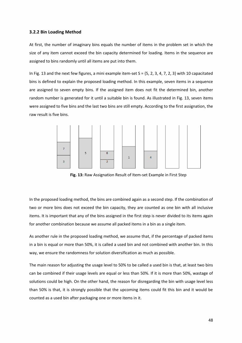
48

3.2.2 Bin Loading Method

At first, the number of imaginary bins equals the number of items in the problem set in which the

size of any item cannot exceed the bin capacity determined for loading. Items in the sequence are

assigned to bins randomly until all items are put into them.

In Fig. 13 and the next few figures, a mini example item-set S = {5, 2, 3, 4, 7, 2, 3} with 10 capacitated

bins is defined to explain the proposed loading method. In this example, seven items in a sequence

are assigned to seven empty bins. If the assigned item does not fit the determined bin, another

random number is generated for it until a suitable bin is found. As illustrated in Fig. 13, seven items

were assigned to five bins and the last two bins are still empty. According to the first assignation, the

raw result is five bins.

Fig. 13: Raw Assignation Result of Item-set Example in First Step

In the proposed loading method, the bins are combined again as a second step. If the combination of

two or more bins does not exceed the bin capacity, they are counted as one bin with all inclusive

items. It is important that any of the bins assigned in the first step is never divided to its items again

for another combination because we assume all packed items in a bin as a single item.

As another rule in the proposed loading method, we assume that, if the percentage of packed items

in a bin is equal or more than 50%, it is called a used bin and not combined with another bin. In this

way, we ensure the randomness for solution diversification as much as possible.

The main reason for adjusting the usage level to 50% to be called a used bin is that, at least two bins

can be combined if their usage levels are equal or less than 50%. If it is more than 50%, wastage of

solutions could be high. On the other hand, the reason for disregarding the bin with usage level less

than 50% is that, it is strongly possible that the upcoming items could fit this bin and it would be

counted as a used bin after packaging one or more items in it.

49

The combination step starts with the first left non-empty bin in line having less than 50% in order to

find a suitable bin through the line. As a result of this phase, there can be only one bin having less

than 50% at most. According to these rules, the combined bins are demonstrated in Fig. 14.

Fig. 14: The Result of Combination Process

Bin-3 and Bin-5 are less than 50% and after the combination process for bins, the modified result is

four bins and the total wastage is 35% as shown in Fig. 15.

Fig. 15: Modified Result of Assignation for Items

All solutions in an initial population are generated by following aforementioned loading rules. After

generating the initial population, neighbourhood function is defined as a tool for the next phase.

3.2.3 Generating a New Solution

In the second phase, all employed bees visit only one solution and generate a new solution from it

by using the neighbourhood function as explained above. In the proposed approach, neighbourhood

function to generate a new solution is explained as follows.

In order to generate a neighbour solution, an item not packed in a fully filled bin is chosen randomly

and packed in another randomly chosen non-empty bin if it fits. In case there is not any suitable bin

for the chosen item, it means that the solution cannot be diversified anymore. In Fig. 16, generating

50

a new solution is demonstrated. After generation, the result may not change for a number of

iterations, however the diversified solution allows for further search.

Fig. 16: Generating a New Solution

There may be some bins that are filled less than 50% after changing the chosen item’s place like

shown in Fig. 16. After moving the item to another bin, the original bin filling level decreased to less

than 50%. In this case, the re-packaging rule in the proposed item is applied again as shown in Fig.

17.

Fig. 17: Modification of Generated Solution

The result of generated solution changed by doing this modification as shown in Fig. 18 with three

bins and 10% wastage. Generating a new solution is also used in onlooker bees phase in the same

way. Proposed bin loading method can be modified with various approaches.

51

Fig. 18: The Modified New Solution

3.2.4 The Roulette Wheel Function

After generating a population for employed bees phase in the ABC algorithm, the roulette wheel

function is used for assigning the onlooker bees to solutions randomly for neighbour search. This

function may send two or more onlooker bees to the same solutions because of randomisation.

In the ABC algorithm, duties of onlooker bees are determined due to their probability value pi

calculated as in equation (5). According to this equation, the solution with high fitness value has a

high chance for selection; however in bin packing problems, low fitness value for wastage is better

to investigate. Because of the minimization purpose of bin packing problems, we need to change the

equation of the roulette wheel function with another one as demonstrated in equation (6) to give a

better chance of a solution with low fitness value.

. (6)

After assignation of onlooker bees to the solution randomly, we apply a neighbourhood search

function for selected solutions the same as in the employed bee phase and then apply greedy search

to select the best fitness value among solutions.

3.2.5 Enhancement with Memory

As a result of greedy neighbourhood search, onlooker bees around the solution selected by roulette

wheel function choose the best fitness value. If they have the information about a worse solution in

their memory, they erase this information and memorize the best solution instead of it.

The ABC algorithm uses a counter to calculate the number of improvement failures. If employed or

onlooker bees improve the solution, the counter for that solution is reset. Otherwise the counter is

increased by one until the predetermined limit. If the counter exceeds this limit, the solution is

52

abandoned; however, it is important that the abandoned solution may be generated and visited

repeatedly. This attribute signifies that the ABC algorithm does not memorize the history of

neighbourhood search whether the abandoned solution is promising or not.

The main purpose of this study is providing the classic ABC algorithm with a memory to avoid

repetition. In this way, the search in the ABC algorithm can escape from possible local optimums.

The proposed “A Memory Embedded ABC Algorithm” works with Short Term Tabu List (STTL)

described in the previous chapter.

According to the proposed algorithm, the abandoned solution is saved in STTL for a predetermined

period. The length of the period depends on the characteristic of tackled item-set, so various lengths

of periods should be tried to obtain better results. It is important that, in the proposed algorithm,

bees do not memorize the move from the original solution to generated solution in greedy search.

They do memorize only unimproved and abandoned solutions. By the agency of memory

reinforcement, solutions that cannot be improved further are prohibited and bees are forced to visit

different solutions for investigation. At the end of the tabu period of listed solutions, they are erased

from the list and can be visited again in case search exigency.

Other operators of the proposed algorithm are the same as the traditional ABC algorithm. In the

next section, the proposed algorithm is described by a computer software implementation.

3.2.6 A Software Implementation for Proposed Algorithm

In this study, MATLAB 2012 software is used for implementations. Item-sets are taken from a

website referred to in the acknowledgement. Item-sets consist of two different distributions with

two different bin capacities. We developed the proposed algorithm by keeping three steps.

Firstly, fundamental algorithms described in section 2.4 are implemented to obtain raw results to

use as a reference point for comparison. Fig. 19.A demonstrates the window for implementation of

the classic algorithm.

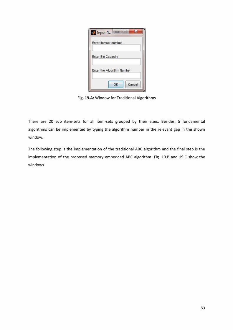
53

Fig. 19.A: Window for Traditional Algorithms

There are 20 sub item-sets for all item-sets grouped by their sizes. Besides, 5 fundamental

algorithms can be implemented by typing the algorithm number in the relevant gap in the shown

window.

The following step is the implementation of the traditional ABC algorithm and the final step is the

implementation of the proposed memory embedded ABC algorithm. Fig. 19.B and 19.C show the

windows.

54

Fig. 19.B: Window for ABC Algorithm Fig. 19.C: Window for Proposed Algorithms

In the next chapter, experiment results obtained by the aforementioned software programmes are

compared and discussed regarding their algorithm and item-set characteristics.

55

Chapter 4: Experimental Results and Discussion

In this chapter, a number of experiments are processed by applying methods which are explained in

previous chapter. Before starting to experiments, we need to understand structures of applied

datasets and then determine default parameter values to obtain sufficient results. After obtaining

experimental results, relevant discussions are provided with overall discussion at the end of chapter.

4.1 Datasets

In this study, there are two classes of 1-D bin packing datasets acquired from [55]. The first 4

datasets consist of items of integer sizes uniformly distributed in (20, 100) to be packed into bins of

size 150. The other 4 datasets consist of triplets of decimal sized items from (25, 50) to be packed

into bins of size 100. For the triplets class, the optimum number of bins is equal to 1/3 of the

number of items.

4.2 Parameter Settings

The main problem in experiments is to determine the default value for the software compilation

process because before an experiment, results cannot be estimated if there is no reference

experiment result. In this study, there are four main parameters: (i) size of bee swarm, (ii) number of

iterations, (iii) number of failures allowance, and (iv) tabu list period for experiments. Different

values were tried to find the best solutions.

The main criterion of value determination is the meaning of parameters for the applied algorithm. At

first, swarm size should be sufficient for the search because the wider the swarm the more initial

solutions. In case of wide swarm selection, researchers would be eligible for a deeper search in the

feasible area. Besides, wider swarm improves the randomisation characteristic of the algorithm by

decreasing the probability of bee placement for food sources in the onlooker phase in the ABC

algorithm. For example, if we choose 50 bees as a swarm size, in the onlooker phase the probability

56

of bee placement for a food source will be 1/50; however, if the swarm size is determined as 100

bees, the probability will decrease to 1/100 for an onlooker bee. In this way, the ABC algorithm can

prevent agglomerating bees in the same food source and allow wider multiple searches.

First experimental results for parameter settings were run to determine parameter values .Fig. 20.A,

20.B, 20.C, 21.A, and 21.B illustrate results of applied parameter values to compare different cases

to determine the best on. Aforementioned five figures (20.A-21.B) show the wastage change as focal

point of this study to be optimised, throughout experimental run represented as number of

iteration. In this study, the swarm size is determined as 50 and 100. According to Table 1, the results

of a 100 bee swarm based search are slightly better than a 50 bee swarm based search in the same

conditions; however, the consumed time is approximately doubled in a 100 bee swarm based

search. On the other hand, according to Table 2, a 50 bee swarm based search obtained better

solutions probably because of the randomisation characteristic.

Table 1: Experiment Results for Dataset-4 Group-7

Table 2: Experiment Results for Dataset-4 Group-1

57

These two tables show that there is no clue whether bee size affects the results or not; however, at

least it is assured that the algorithm makes a deeper search with a 100 bee swarm parameter. On

the other hand, wider swarm could be determined but the consumed time will be increased by

assigning a higher number of bees. As a result, in this study a 100 bee swarm is determined as the

default parameter value.

The number of iterations is also an important parameter for a search because little iteration can

mislead us about the outputs of experiments. On the other hand, researchers should avoid an

unnecessary number of iterations to save time.

In this study, various experiments were run to determine the default parameter value for the

number of iterations. Dataset-4 (the widest dataset in this study to process with 1000 items) is

considered due to its size because it requires more iteration to make the result graph reach a stable

condition. Fig. 20.A, 20.B and 20.C show the tendency of the result. In Fig. 20.A; the graph does not

reach its stability with 5,000 iterations; however, in Fig. 20.C; 10,000 iterations was tried and the

graph reaches its approximate stability. Finally, 7,500 iterations were tried and in Fig. 20.C the result

also reached its approximate stability. As a result, in this study, 7,500 iterations is determined as the

default parameter value and applied for all datasets.

Another parameter of experiments is the number of failure allowance for neighbourhood search

performed by bees. If a small number of failure allowances are determined as a default value, bees

cannot perform a further neighbourhood search around the source in the ABC algorithm and cannot

find possible better solutions. On the other hand, if a high number of failure allowances are

determined, bees do not seek another source and it may cause unnecessary time consumption.

58

Fig. 20.A: 5000 Iteration Experiment for Dataset-4 Group-7

Fig. 20.B: 7500 Iteration Experiment for Dataset-4 Group-7

59

Fig. 20.C: 10000 Iteration Experiment for Dataset-4 Group-7

In this study, as a first step the number of failure allowances is determined as 3 and 5 as shown in

table-1 and table-2; however, a further search by applying a higher number of failures shows that,

the applied algorithm requires a higher allowance to obtain better solutions. The effect of a high

number can be observed even in comparison between 3 and 5 allowance as shown in table-3.

Table 3: The Effect of the Number of Failure Allowance in Same Group in Dataset-4

The average optimum number of bins with 5 failure allowance in group-17 is 425.60; however, it

increased to 430.60 when the number of failures was determined as 3. Fig. 21.A and 21.B also show

the effect of failure allowance determined as 100 and 1000 respectively with 5,000 iterations.

60

Fig. 21.A: 100 Failure Experiment for Dataset-4 Group-7

Fig. 21.B: 1,000 Failure Allowance Experiment for Dataset-4 Group-7

Throughout 5,000 iterations, the ABC algorithm search obtains the same minimum value of 0.0295;

however, the 50 failure allowance experiment obtains a worse result with 0.0315. According to

61

table-3 and Fig. 21.A and 21.B results improve while the number of maximum failures increases until

100 failures. Over this value, the ABC algorithm cannot show a significant difference. As a result, the

number of maximum failures is determined as 100.

The last important parameter is the period of an item saved in the tabu list. In fact, various tabu

periods were tried for experiments yet there is no significant better solution in comparison with the

traditional ABC algorithm and very few solutions are saved in memory. On the other hand, we need

to observe the effect of the tabu list on experiments and investigate the tendency of the proposed

approach by the agency of result graphs.

In this study, the length of the period is determined as 1500 iterations which equal 20% of the total

number of iterations.

4.3 Experimental Results

There are 8 item-sets which consist of 120, 250, 500, 1000, 60, 120, 249, and 501 items respectively.

Experiments were executed in three phases: traditional algorithm results, classic ABC algorithm

results, and memory embedded ABC algorithm results.

In following pages in this part; whole figures represent experimental results of applied algorithms by

graphs for 8 different item-sets. Results are introduced by average number of bins and average

wastage change throughout experimental runs represented as number of iteration.

4.3.1 Results for Traditional Algorithms

In the first phase, 5 different traditional algorithms were applied on all sub-groups of item-sets. Each

item-set consists of 20 sub-groups. Results of the first four item-sets and second four item-sets show

different attitudes due to their distribution and integrity characteristics. Only two of the eight item-

sets are demonstrated in table-4.A and table-4.B for the raw results of traditional 1-D bin packing

algorithms. The rest of traditional 1-D bin packing results can be seen in Appendix A between page

84 and 91 by eight different tables.

Yellow highlighted rows represent randomly chosen sub-groups shown at the left side of tables, for

implementation in second and last phase. “LS” represents list size of sub-groups and “Cap.”

represents the capacity of bins. At the top of results, applied algorithms are illustrated in green

boxes. Wastage values for best solutions are not provided because the website [55] only provides

the best number of bins.

62

Table-4.A: Results of Traditional 1-D Bin Packing Algorithms for Itemset-4

Table-4.B: Results of Traditional 1-D Bin Packing Algorithms for Itemset-8

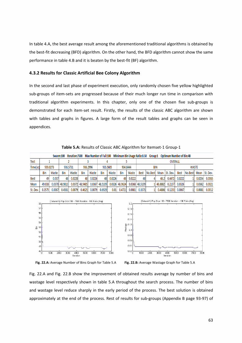
63

In table 4.A, the best average result among the aforementioned traditional algorithms is obtained by

the best-fit decreasing (BFD) algorithm. On the other hand, the BFD algorithm cannot show the same

performance in table 4.B and it is beaten by the best-fit (BF) algorithm.

4.3.2 Results for Classic Artificial Bee Colony Algorithm

In the second and last phase of experiment execution, only randomly chosen five yellow highlighted

sub-groups of item-sets are progressed because of their much longer run time in comparison with

traditional algorithm experiments. In this chapter, only one of the chosen five sub-groups is

demonstrated for each item-set result. Firstly, the results of the classic ABC algorithm are shown

with tables and graphs in figures. A large form of the result tables and graphs can be seen in

appendices.

Table 5.A: Results of Classic ABC Algorithm for Itemset-1 Group-1

Fig. 22.A: Average Number of Bins Graph for Table 5.A Fig. 22.B: Average Wastage Graph for Table 5.A

Fig. 22.A and Fig. 22.B show the improvement of obtained results average by number of bins and

wastage level respectively shown in table 5.A throughout the search process. The number of bins

and wastage level reduce sharply in the early period of the process. The best solution is obtained

approximately at the end of the process. Rest of results for sub-groups (Appendix B page 93-97) of

64

Itemset-1 show same attitudes with graphs in Fig. 22.A and Fig. 22.B but the obtained number of

bins because of total value of items in sub-groups.

Table 5.B: Results of Classic ABC Algorithm for Itemset-2 Group-5

Fig. 23.A: Average Number of Bins Graph for Table 5.B Fig. 23.B: Average Wastage Graph for Table 5.B

The tendency of Fig. 23.A and Fig. 23.B show the same attitudes with Fig. 22.A and Fig. 22.B;

however, it takes more time to reach stability probably because of the size of the item-set. Besides,

the search obtains the best solution at iteration 3000 approximately conversely results of other sub-

groups of itemset-2 (Appendix B page 98-102) because other sub-groups obtain the best results

before 3000 iteration.

The experiment groups were executed once in itemset-3, itemset-4, and itemset-8 because the run

times are too long and according to the aim of the graphs, obtained results can be considered as

average results. The results of the aforementioned item-sets are demonstrated in table 5.C.

Table 5.C: Results of Classic ABC Algorithm for Itemset-3, Itemset-4, and Itemset-8

BIN WASTAGE (%) TIME (sec)

ABC IS-3 Gr-3 100-7500-100 207 0.0280 5.8826e+03

ABC IS-4 Gr-1 100-7500-100 411 0.0306 1.4936e+04

ABC IS-8 Gr-8 100-7500-100 175 0.0473 6.1104e+03

65

Fig. 24.A: Average No. of Bins Graph for IS-3 in Table 5.C Fig. 24.B: Average Wastage Graph for IS-3 in Table 5.C

According to Fig. 24.A and Fig. 24.B, the search process reaches its stability at iteration 2000

approximately and shows a more proper presentation in comparison with the previous two item-

sets by a reduction in the number of zig zags. The search obtains its best result at the mid-process.

Fig. 25.A: Average No. of Bins Graph for IS-4 in Table 5.C Fig. 25.B: Average Wastage Graph for IS-4 in Table 5.C

The most proper graphs in the first four item-sets with much fewer zig zags are Fig. 25.A and Fig.

25.B. As seen in the graphs, they reach their stable condition later than others because the item

exchange rate in wide sized item-set is smaller than others and this exchange may not be observed

in graphs. Even 7500 iterations would not be enough to find the algorithm’s best solution because

the stable condition cannot be observed for a long period.

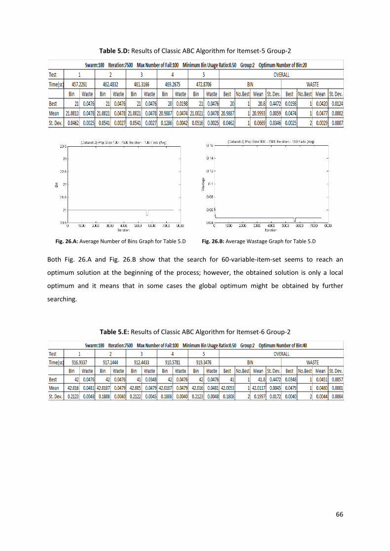
66

Table 5.D: Results of Classic ABC Algorithm for Itemset-5 Group-2

Fig. 26.A: Average Number of Bins Graph for Table 5.D Fig. 26.B: Average Wastage Graph for Table 5.D

Both Fig. 26.A and Fig. 26.B show that the search for 60-variable-item-set seems to reach an

optimum solution at the beginning of the process; however, the obtained solution is only a local

optimum and it means that in some cases the global optimum might be obtained by further

searching.

Table 5.E: Results of Classic ABC Algorithm for Itemset-6 Group-2

67

Fig. 27.A: Average Number of Bins Graph for Table 5.E Fig. 27.B: Average Wastage Graph for Table 5.E

In contradistinction to Fig. 26.A and Fig. 26.B, in Fig. 27.A and Fig. 27.B; graphs obtain their best

solution in the early period of the process. However, the graph reaches a stable condition with

worse solution and never obtains the best solution again. Graphs of other sub-groups of itemset-6

(Appendix B page 114-118) show same attitudes but change characteristic. They also obtain best

solution in early period however; they reach stabile condition in late period with more zig zags.

Table 5.F: Results of Classic ABC Algorithm for Itemset-7 Group-1

Fig. 28.A: Average Number of Bins Graph for Table 5.F Fig. 28.B: Average Wastage Graph for Table 5.F

Fig. 28.A and Fig. 28.B show the same characteristic as graphs of itemset-6 but a higher number of

zig zags.

68

Fig. 29.A: Average No. of Bins Graph for IS8 in Table 5C Fig. 29.B: Average Wastage Graph for IS8 in Table 5.C

In Fig. 29.A and Fig. 29.B; graphs obtain the best solution near iteration 2000. Like the previous

graphs of the two item-set (6 and 7), the graph for results of itemset-8 achieves stability with a

worse solution. The possible reason for this condition is that, in the ABC algorithm we also substitute

a new solution instead of the best solution of the current iteration after 100 failures. On the other

hand, the algorithm in which we do not replace the best solution of iteration, cannot obtain any

better solution in comparison with the current method.

The ABC algorithm search in the second four item-sets obtains the best solution earlier than the first

ones due to the distribution difference between them. It means that items in the second four item-

sets could be packed easier.

According to the results of the classic ABC algorithm, it is capable of showing a better performance

in comparison with traditional 1-D bin packing algorithms; however, the BFD algorithm beats the

classic ABC algorithm for first item-sets and obtains the best results. In contrast, the BFD algorithm

shows a much worse performance and it is even beaten by the best fit (BF) algorithm which obtains

worse results than the classic ABC algorithm for all item-sets.

4.3.3 Results for Memory Embedded Artificial Bee Colony (MEABC) Algorithm

The reason for this condition is probably linked to characteristics of item-sets. As defined above, two

different distributed grouped item-sets consist of integer and decimal sized items. Obtained results

show that the BFD algorithm cannot show sufficient performance with decimal sized items. The

possible reason for this condition is that, if decimal sized items are sorted in a descended trend,

items may not be allocated in bins because the same fractioned numbers possibly cannot be

assembled easily. On the other hand, different fractioned numbers might be assembled with higher

possibility in comparison with the mentioned arrangement. As a next and last step, the results of the

proposed memory embedded artificial bee colony (MEABC) algorithm are illustrated in table 6.A.

69

Table 6.A: Results of Memory Embedded ABC Algorithm for Itemset-1 Group-1

Fig. 30.A: Average Number of Bins Graph for Table 6.A Fig. 30.B: Average Wastage Graph for Table 6.A

According to results in table 6.A, the MEABC algorithm obtains the exact solution like the classic ABC

algorithm because of the smallness of the item-set size. This condition changes in next experiments

with an increase in wastage level. In Fig. 30.A and 30.B; graphs obtain the best solution of the

process at near iteration 1000 and then they are stabilized with a worse solution. Conversely, other

sub-groups of itemset-1 (Appendix C page 129-132) reach their stabile condition earlier than sub-

group 1 however; sub-group 17 shows sharp change at the end of experiment run. This means that,

proposed method may be executed for more iteration.

Table 6.B: Results of Memory Embedded ABC Algorithm for Itemset-2 Group-5

70

Fig. 31.A: Average Number of Bins for Table 6.B Fig. 31.B: Average Wastage for Table 6.B

Like other results, in Fig. 31.A and Fig. 31.B; both graphs tend to achieve stability after an amount of

iterations. The straight line of the graphs could be considered as the average of the results if it is

achieved in a short time. According to the graphs above, the best solution of the experiment is

obtained at near iteration 7000 and then the graphs return to the straight line representing a worse

solution after a number of iterations.

Table 6.C: Results of Memory Embedded ABC Algorithm for Itemset-3, Itemset-4, and Itemset-8

Fig. 32.A: Average No. of Bins Graph for IS3 in Table 6C Fig. 32.B: Average Wastage Graph for IS3 in Table 6C

The results of the MEABC algorithm for itemset-3 are the same as the results of the ABC algorithm

and the graphs show the same characteristics. It means that the memory system does not affect the

ABC algorithm search results. Besides, MEABC results for sub-group 13 (Appendix B, page 93, Table

11) of itemset-3 obtains better solution than classic ABC algorithm as an exception. Itemset-3,

itemset-4 and itemset-8 consist of large number of items and run times for them are much longer

BIN WASTAGE (%) TIME (sec)

MEABC IS-3 Gr-3 100-7500-100 207 0.0280 5.7224e+03

MEABC IS-4 Gr-1 100-7500-100 411 0.0306 1.4848e+04

MEABC IS-8 Gr-8 100-7500-100 175 0.0473 6.1104e+03

71

than others and because of this circumstance each experiment is run once. In this case, exceptional

results are obtained just for aforementioned item-sets because of randomness.

Fig. 33.A: Average No. of Bins Graph for IS4 in Table 6C Fig. 33.B: Average Wastage Graph for IS4 in Table 6C

In Fig. 33.A and 33.B; both graphs also show the same performance as the classic ABC algorithm

search results and cannot differentiate the obtained results.

Table 6.D: Results of Memory Embedded ABC Algorithm for Itemset-5 Group-2

Fig. 34.A: Average Number of Bins Graph for Table 6.D Fig. 34.B: Average Wastage Graph for Table 6.D

The graph of average results for itemset-5 with the MEABC algorithm search is slightly different from

the graph of the ABC algorithm search due to the increased number of plunges in the graph. On the

other hand, graphs in Fig. 34.A and 34.B can be considered as unstable in comparison with graphs of

other sub-groups of itemset-5 (Appendix C page 144-147).

72

Table 6.E: Results of Memory Embedded ABC Algorithm for Itemset-6 Group-2

Fig. 35.A: Average Number of Bins Graph for Table 6.E Fig. 35.B: Average Wastage Graph for Table 6.E

In contradistinction to all other graphs, in Fig. 35.A and 35.B; graphs show interesting characteristics

with two different straight lines. The trend of the second line observed after iteration 5000

represents a worse solution than the previous worse solution in comparison with the obtained best

solution and cannot be fixed until the end of the process. In spite of this, the global optimum is the

same as the solution obtained by ABC algorithm search.

Table 6.F: Results of Memory Embedded ABC Algorithm for Itemset-7 Group-1

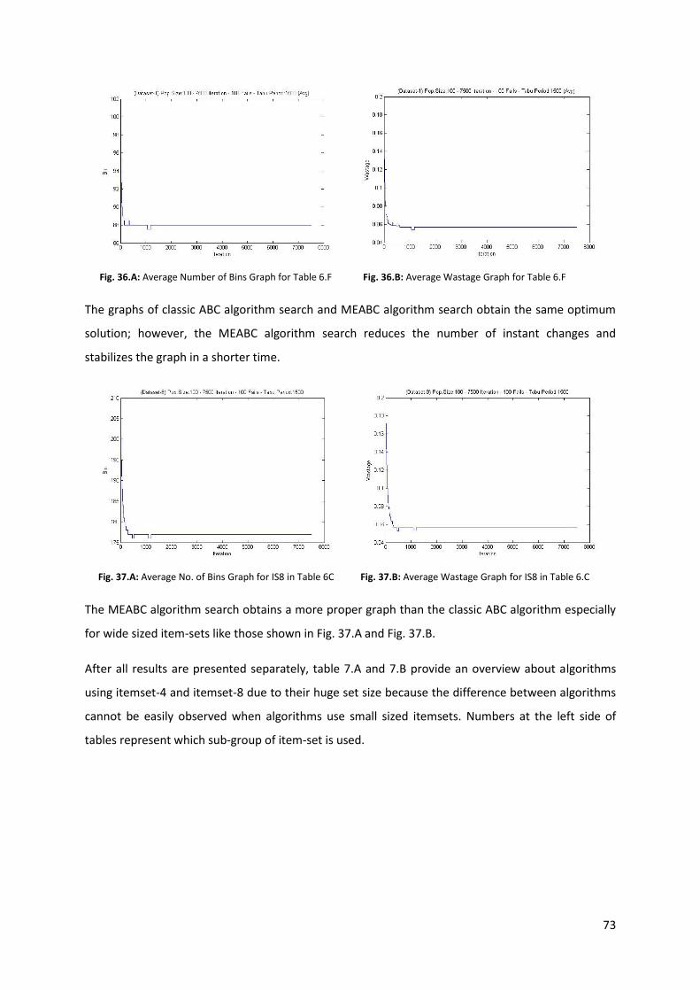
73

Fig. 36.A: Average Number of Bins Graph for Table 6.F Fig. 36.B: Average Wastage Graph for Table 6.F

The graphs of classic ABC algorithm search and MEABC algorithm search obtain the same optimum

solution; however, the MEABC algorithm search reduces the number of instant changes and

stabilizes the graph in a shorter time.

Fig. 37.A: Average No. of Bins Graph for IS8 in Table 6C Fig. 37.B: Average Wastage Graph for IS8 in Table 6.C

The MEABC algorithm search obtains a more proper graph than the classic ABC algorithm especially

for wide sized item-sets like those shown in Fig. 37.A and Fig. 37.B.

After all results are presented separately, table 7.A and 7.B provide an overview about algorithms

using itemset-4 and itemset-8 due to their huge set size because the difference between algorithms

cannot be easily observed when algorithms use small sized itemsets. Numbers at the left side of

tables represent which sub-group of item-set is used.

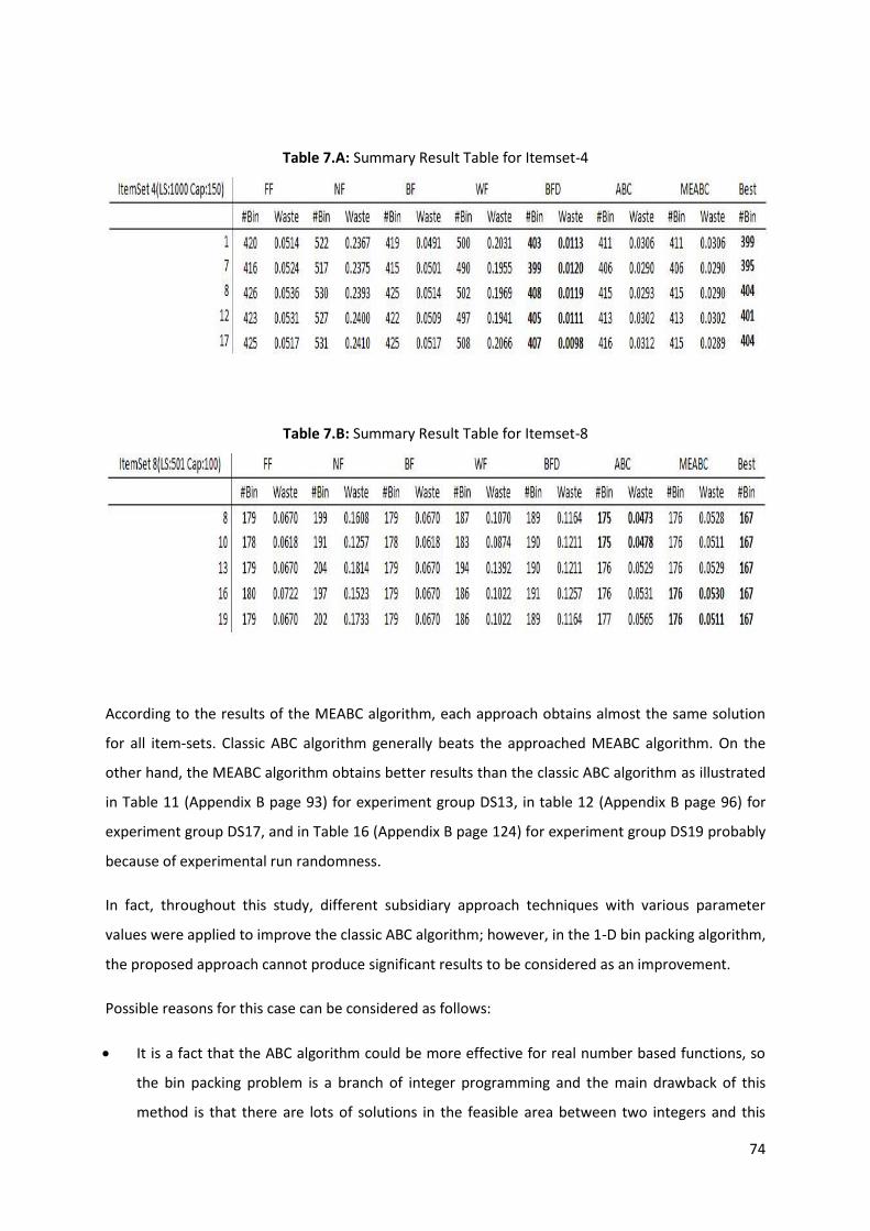
74

Table 7.A: Summary Result Table for Itemset-4

Table 7.B: Summary Result Table for Itemset-8

According to the results of the MEABC algorithm, each approach obtains almost the same solution

for all item-sets. Classic ABC algorithm generally beats the approached MEABC algorithm. On the

other hand, the MEABC algorithm obtains better results than the classic ABC algorithm as illustrated

in Table 11 (Appendix B page 93) for experiment group DS13, in table 12 (Appendix B page 96) for

experiment group DS17, and in Table 16 (Appendix B page 124) for experiment group DS19 probably

because of experimental run randomness.

In fact, throughout this study, different subsidiary approach techniques with various parameter

values were applied to improve the classic ABC algorithm; however, in the 1-D bin packing algorithm,

the proposed approach cannot produce significant results to be considered as an improvement.

Possible reasons for this case can be considered as follows:

It is a fact that the ABC algorithm could be more effective for real number based functions, so

the bin packing problem is a branch of integer programming and the main drawback of this

method is that there are lots of solutions in the feasible area between two integers and this

75

method cannot benefit these solutions. In the 1-D bin packing problem, algorithms from

literature may not find the actual solution.

Both algorithms restrict the search by using the counter operator in classic ABC algorithm and

tabu period in the proposed MEABC algorithm. These operators may prevent a further search in

the feasible area.

The classic and proposed algorithm might require a higher number of iterations to reach the

optimum solution; however, in this case the application of these algorithms can reach a high

cost. At least the mentioned algorithm run times should be reasonably short to be considered

as a candidate run time because traditional algorithms solve the problem in a very short time.

The classic ABC algorithm also has its own control parameter unlike in Pham et al.’s bees

algorithm. In this case, it is unavoidable that both classic ABC algorithm and proposed MEABC

algorithm obtain the same optimum solutions. Although the MEABC algorithm proposes a

better memory system, the classic ABC algorithm also has a kind of immature short term

memory. According to all the results, it seems that the classic ABC algorithm developed by

Karaboga does not require a memory system at least for integer programming.

76

Chapter 5: Conclusion

In this study, one of the common NP-hard Knapsack problems, the 1-D bin packing problem, is

handled to improve the standard results obtained by well-known packing algorithms from literature

with new approaches. Deterministic methods do not show sufficient performance for the tackled

complex type bin packing problem. In order to fulfil this purpose, one of the heuristic approaches is

applied instead of a deterministic approach to overcome the mentioned difficulty.

Recent research about heuristic optimisation has achieved various outcomes such as new

approximation methods for complex problems and one of those outcomes is an artificial bee colony

(ABC) algorithm based on swarm intelligence, developed by Karaboga in 2005, and applied on

several functions and problems. As a result, we are interested in the ABC algorithm based on past

studies about it.

In fact, the main purpose of this study is to make an improvement on the classic ABC algorithm. In

the first phase of study, traditional bin packing algorithms were investigated and applied on various

item-sets. After this phase, the ABC algorithm was applied on the same item-sets to observe the

difference between results of swarm based search and results of fixed traditional algorithm

searches.

In order to advance the classic ABC algorithm, we investigated its possible drawbacks and

deficiencies. There are two salient drawbacks of ABC algorithm which are randomisation and

repetition referred in section 3.1.

As a result of this investigation, an enhancement with memory which is based on restriction for

repetitive failures by saving them in a list in order to escape from possible local optimums was

determined as a starting point for improvement.

In the last phase of the study, the proposed approach which is a modified form of the classic ABC

algorithm was applied on the same item-sets to observe the difference. According to the obtained

results, the classic ABC algorithm and proposed memory embedded artificial bee colony (MEABC)

algorithm can be considered as strong candidates to solve 1-D bin packing problems in comparison

with traditional 1-D bin packing algorithms. Both algorithms beat traditional algorithms when they

77

are applied on triplet sets (itemset-5, 6, 7, 8) however; they cannot show same performance when

they are applied on normal distributed sets (itemset-1, 2, 3, 4). Besides, it takes a much longer time

to reduce the wastage to the percentage obtained by traditional algorithms. In other words, in order

to obtain a better solution than traditional algorithms, we have to tolerate run time.

When we focus on differences between the classic ABC algorithm and proposed MEABC algorithm,

memory enhancement cannot differentiate the results of the classic ABC algorithm in an overall

outlook. However, a few experiments could be considered as exceptions because of the randomness

characteristic explained in previous chapter.

On the other hand, the proposed idea about the ABC algorithm could be applied on various real

valued functions rather than integer programming like the tackled problem in this study because

generating a new solution for an improvement in the search is restricted by integer values. In case of

unrestricted search, the proposed algorithm would be more effective.

In addition, we restricted the search to 7500 iterations which is determined by several trials and we

cannot estimate how much iteration is required especially by itemset-4 to obtain an exact solution.

It is possible that both classic ABC algorithm and proposed MEABC algorithm may obtain the global

optimum but it would also take a very long time and this condition would not be found practical by

executors. Saving one more bin by a further search over a long period of time would not be

acceptable so, in this case, we also need to optimise the run time.

It is a fact that Pham et al.’s bees algorithm does not involve a control parameter. In this case, the

proposed idea can increase the performance of Pham et al.’s bees algorithm. On the other hand,

Pham et al. [30] separate bees in onlooker bee phase in order to their performance value and

choose bees for next phase from promising and unpromising ones in a rate. This speciality may

increase the performance of ABC algorithm in same phase [29]. In fact, these two conditions would

be adjunct factors for each ABC and Bees algorithms.

In this study, we focus on memorising the unpromising solutions to avoid hill climbing. According to

tabu list idea, proposed algorithm just saves unpromising solutions for a period however, proposed

algorithm does not categorise mentioned solutions when applied on classic ABC algorithm. In this

case, it is possible that, applied algorithm may generate a huge number of unpromising solutions

that not eligible for obtaining global optimum. Instead, we can decrease the number of processed

solutions by categorising according to performance quality. On the other hand, decreasing the

number of processed solution by using this method may cause a hill climbing easier than

randomisation method however; we can solve this problem by using memory system again.

78

Xiang and An [38] propose a chaotic initialisation method in which initial population in next iteration

is subject to current population, to make applied algorithm more robust. Same technique can be

applied on ABC algorithm for an alternative improvement. Moreover, chaotic initialisation method

can be combined with Pham et al.’s choice system and then a memory system like proposed in this

study can be integrated to this combined algorithm. On the other hand, memory idea is able to be

applied on each aforementioned algorithm separately.

All these proposals show that, we can reinforce current ABC algorithm and proposed MEABC

algorithm with aforementioned beneficial structures of other algorithms for further improvements.

As a result, the proposed idea is promising by having a memory system so; it would be applicable for

other algorithms beside Karaboga’s ABC algorithm [29]. However, we need to consider the structure

of the tackled problem firstly, and then we can determine how to integrate a memory system to

chosen applied algorithms.

79

References

[1] Turajli´c, N., and Dragovi´c, I., (2012), “A Hybrid Metaheuristic Based on Variable

Neighbourhood Search and Tabu Search for the Web Service Selection Problem”, Electronic

Notes in Discrete Mathematics, 39, pp. 145-152.

[2] Li, C., Liao, X., and Yu, J., (2004), “Tabu Search for Fuzzy Optimization and Applications”,

Information Sciences, 158, pp. 3-13.

[3] Mousavi, M. A., Masouleh, M. T., and Karimi, A., (2014), "On the maximal singularity-free

ellipse of planar 3-RPR parallel mechanism via convex optimization", Robotics and

Computer-Integrated Manufacturing, 30, pp.218-227.

[4] Cavazutti, M., (2013), Optimization Methods: From Theory to Design, pp.77-78.

[5] Ming-Hua, L., Jung-Fa, T., and Chian-Son, Y., (2012), "A Review of Deterministic Optimization

Methods in Engineering and Management", Mathematical Problems in Engineering, 2012,

Article ID 756023, pp. 1-15.

[6] Skiborowski, M., Rautenberg, M., Marquardt, W., (2013), "A novel approach to hybrid

evolutionary-deterministic optimization in process design", Computer Aided Chemical

Engineering, 32, pp. 961-966.

[7] Marcovecchio, M. G., and Novais, A. Q., (2011), "A deterministic optimization approach for

the unit commitment problem", Computer Aided Chemical Engineering, 29, pp. 532-536.

[8] Trindade, G., and Ambrosio, J., (2012), "An optimization method to estimate models with

store-level data: A case study", European Journal of Operational Research, 127(3), pp. 664-

672.

[9] Sulaiman, E., Ahmad, M.Z., Kosaka, T., Matsui, N., (2013), "Design Optimization Studies on

High Torque and High Power Density Hybrid Excitation Flux Switching Motor for HEV",

Procedia Engineering, 53, pp. 312-322.

[10] Carvalho, J.M.V., (2002), "LP models for bin packing and cutting stock problems", European

Journal of Operational Research, 141(2), pp. 253-273.

[11] Lee, K.Y., El-Sharkawi, M.A., (2008), Modern Heuristic Optimization Tehcniques, pp. I-XXVIII.

[12] Karaboga, D., (2011), "Bolum 1 - Giris", Yapay Zeka Optimizasyon Algoritmalari, pp. 1-19.

[Turkish]

[13] Kovacevic, M., Madic, M., and Radovanovic, M., (2013), "Software prototype for validation

of machining optimization solutions obtained with meta-heuristic algorithms", Expert

Systems with Applications, 40(17), pp. 6985-6996.

[14] Li, Z., Tian, Z., Xie, Y., Huang, R., and Tan, J., (2013), "A knowledge-based heuristic particle

swarm optimization approach with the adjustment strategy for the weighted circle packing

problem", Computers & Mathematics with Applications, 66(10), pp. 1758-1769.

80

[15] Liu, W., and Xing, L., (2014), "The double layer optimization problem to express logistics

systems and its heuristic algorithm", Expert Systems with Applications, 41(1), pp. 237-245.

[16] Kaveh, A., and Khayatazad, M., (2012), "A new meta-heuristic method: Ray Optimization",

Computers & Structures, 112-113, pp. 283-294.

[17] Min, B., Lewis, J., Matson, E.T., and Smith, A.H., (2013), "Heuristic optimization techniques

for self-orientation of directional antennas in long-distance point-to-point broadband

networks", Ad Hoc Networks, 11(8), pp. 2252-2263.

[18] Karaboga, D., (2011), "Bolum 4 - Genetik Algoritma", Yapay Zeka Optimizasyon Algoritmalari,

pp. 73-108. [Turkish]

[19] Arora, J.S., (2012), "Chapter 16 – Genetic Algorithms for Optimum Design", Introduction to

Optimum Design (Third Edition), pp. 643-655.

[20] Goncalves, J.F., Resende, M.G.C., (2013), "A biased random key genetic algorithm for 2D and

3D bin packing problems", International Journal of Production Economics, 145(2), pp. 500-

510.

[21] Das, S., Mallipeddi, R., Maity, D., (2013), "Adaptive evolutionary programming with p-best

mutation strategy", Swarm and Evolutionary Computation, 9, pp.58-68.

[22] Tajuddin, M.F.N., Ayob, S.M., Salam, Z., and Saad, M.S., (2013), "Evolutionary based

maximum power point tracking technique using differential evolution algorithm", Energy

and Buildings, 67, pp. 245-252.

[23] Sahu, A., Panigrahi, S.K., and Pattnaik, S., (2012), "Fast Convergence Particle Swarm

Optimization for Functions Optimization", Procedia Technology, 4, pp. 319-324.

[24] Karaboga, D., (2011), "Bolum 8 - Parcacik Suru Optimizasyonu", Yapay Zeka Optimizasyon

Algoritmalari, pp. 182-197. [Turkish]

[25] Columbus, C.C., Chandrasekaran, K., and Simon, S.P., (2012), "Nodal and calony optimization

for solving profit based unit commitment problem for GENCOs", Applied Soft Computing, 12,

pp. 145-160.

[26] Fuellerer, G., Doerner, K.F., Hartl, R.F., and Iori, M., (2009), "Ant colony optimization for the

two-dimensional loading vehicle routing problem", Computers & Operations Research,

36(3), pp. 655-673.

[27] Singh, M.P., Dixit, R.S., (2013), "Optimization os stochastic networks using simulated

annealing for the storage and recalling of compressed images using SOM", Engineering

Applications of Artificial Intelligence, 26, pp. 2383-2396.

[28] Rao, R.L., Iyengar, S.S., (1994), "Bin-packing by simulated annealing", Computers &

Mathematics with Applications, 27(5), pp. 71-82.

[29] Karaboga, D., (2005), "An idea based on honey bee swarm for numerical optimization",

University Engineering Faculty COmputer Engineering Department Technical Report-TR06.

81

[30] Pham, D.T., Ghanbarzadeh, A., Koc, E., Otri, S., Rahim, S., Zaidi, M., (2006), "The Bees

Algorithm - A Novel Tool for Complex Optimisation Problems", Technical Note,

Manufacturing Engineering Centre, Cardiff University, UK.

[31] Karaboga, D., and Ozturk, C., (2011), "A novel clustering approach: Artificial Bee Colony

(ABC) algorithm", Applied Soft Computing, 11, pp. 652-657

[32] Akay, B., Karaboga, D., (2012), "A modified Artificial Bee Colony algorithm for real-parameter

optimization", Information Sciences, 192, pp. 120-142.

[33] Xu, S., Ji, Z., Pham, D.T., Yu, F., (2010), "Bio-Inspired Binary Bees Algorithm for a Two-Level

Distribution Optimisation Problem", Bionic Engineering, 7, pp. 161-167.

[34] Dereli, T., Das, G.S., (2011), "A hybrid bees algorithm for solving container loading

problems", Applied Soft Computing, 11,pp. 2854-2862.

[35] Kang, F., Li, J., Li, H., (2013), "Artificial bee colony algorithm and pattern search hybridized

for global optimization", Applied Soft Computing, 13, pp. 1781-1791.

[36] Ozbakir, L., Baykasoglu, A., and Tapkan, P., (2010), "Bees algorithm for generalized

assignment problem", Applied Mathematics and Computation, 215, pp. 3782-3795.

[37] Gao, W., and Liu, S., (2011), "Improved artificial bee colony algorithm for global

optimization", Information Processing Letters, 111, pp. 871-882.

[38] Xiang, W., An, M., (2013), "An efficient and robust artificial bee colony algorithm for

numerical optimization", Computers and Operation Research, 40, pp. 1256-1265.

[39] Szeto, W.Y., Wu, Y., and Ho, S.C., (2011), "An artificial bee colony algorithm for the

capacitated vehicle routing problem", European Journal of operational Research, 215, pp.

126-135.

[40] Karaboga, D., and Akay, B., (2009), "A comparative study of Artificial Bee Colony algorithm",

Applied Mathematics and Computation, 214, pp. 108-132. [Turkish]

[41] Von Frisch, K., (1973), "Decoding the Language of the Bee", Nobel Lecture, December 12,

[PDF]: http://nobelprize.org/nobel_prizes/medicine/laureates/1973/frisch-lecture.pdf

[42] Karaboga, D., (2011), "Bolum 3 - Tabu Arastirmasi Algoritmasi", Yapay Zeka Optimizasyon

Algoritmalari, pp. 47-71. [Turkish]

[43] Mashinchi, M.H., Orgun, M.A., and Pedrycz, W., (2011), "Hybrid optimization with improved

tabu search", Applied Soft Computing, 11, pp. 1993-2006.

[44] Ji, M., and Tang, H., (2004), "Global optimizations and tabu search based on memory",

Applied Mathematics and Computation, 159, pp. 449-457.

[45] Ahonen, H., de Alvarenga, A.G., and Amaral, A.R.S., (2014), "Simulated annealing and tabu

search approach for the Corridor Allocation Problem", European Journal of Operational

Research, 232(1), pp. 221-233.

82

[46] Belle, J.V., Valckenaers, P., Berghe, G.V., Cattrysse, D., (2013), "A tabu search approach to

the truck scheduling problem with multiple docks and time windows", Computers and

Industrial Engineering, 66(4), pp. 818-826.

[47] Jia, H., Li, Y., Dong, B., and Ya, H., (2013), "An Improved Tabu Search Approach to Vehicle

Routing Problem", Procedia - Social and Behavioral Sciences, 96(6), pp. 1208-1217.

[48] Tao, Y., Wang, F., (2013), "An effective tabu search approach with improved loading

algorithms for the 3L-CVRP", Computers and Operations Research, In Press, Corrected Proof

[49] Berberler, M.E., Nuriyev, U., and Yildirim, A., (2011), "A software for the one-dimensional

cutting stock problem", Journal of King Saud University, 23, pp. 69-76.

[50] Loh, K., Golden, B., and Wasil, E., (2008), "Solving the one-dimensional bin packing problem

with a weight annealing heuristic", Computers and Operations Research, 35(7), pp. 2283-

2291.

[51] Xavier, E.C., and Miyazawa, F.K., (2008), "A one-dimensional bin packing problem with shelf

divisions", Discrete Applied Mathematics, 156(7), pp. 1083-1096.

[52] Zhang, Z., Guo, S., Zhu, W., Oon, W.C., and Lim, A., (2012), "Space defragmentation for

packing problems", European Journal of Operational Research, 222(3), pp. 452-463.

[53] Epstein, L., and Levy, M., (2010), "Dynamic multi-dimensional bin packing", Journal of

Discrete Algorithms, 8(4), pp. 356-372.

[54] Hifi, M., Kacem, I., Negre, S., and Wu, L., (2010), "A Linear Programming Approach for the

Three-Dimensional Bin-Packing Problem", Electronic Notes in Discrete Mathematics, 36, pp.

993-1000.

[55] http://people.brunel.ac.uk/~mastjjb/jeb/orlib/binpackinfo.html last accessed at 20.30 on

08.02.2014

[56] http://mrking.cmswiki.wikispaces.net/file/view/BinPacking.docx last accessed at 20.35 on

08.02.2014

[57] http://en.wikipedia.org/wiki/Convex_set last accessed at 20.42 on 08.02.2014

[58] http://chern.ie.nthu.edu.tw/gen/10.pdf%E2%80%8E last accessed at 20.40 on 08.02.2014

[59] Stein, O., Oldenburg, J., and Marquardt, W., (2004), “Continuous reformulation of discrete-

continuous optimization problems”, Computers and Chemical Engineering, 28(10), pp. 1951-

1966.

[60] Ford, J., A., (1991), “On the conditioning of the Hessian approximation in quasi-Newton

methods”, Journal of Computational and Applied Mathematics, 35(1-3), pp. 197-206

83

Appendix A

84

Table-1: Results of Traditional 1-D Bin Packing Algorithms for Itemset-1

Data Set (LS:120 Cap:150) First-Fit Next-Fit Best-Fit Worst-Fit Best-Fit

Decreasing Best

Solution

#Bin Waste #Bin Waste #Bin Waste #Bin Waste #Bin Waste #Bin

1 50 0.0563 64 0.2627 51 0.0748 59 0.2002 49 0.037 48

2 51 0.0582 63 0.2376 51 0.0582 61 0.2126 49 0.0197 49

3 48 0.0564 57 0.2054 48 0.0564 57 0.2054 47 0.0363 46

4 52 0.066 65 0.2528 53 0.0836 63 0.2291 50 0.0287 49

5 52 0.0572 64 0.234 52 0.0572 64 0.234 50 0.0195 50

6 52 0.0869 61 0.2216 52 0.0869 58 0.1814 49 0.031 48

7 51 0.0671 63 0.2448 51 0.0671 59 0.1936 49 0.029 48

8 52 0.0647 63 0.228 52 0.0647 60 0.1894 50 0.0273 49

9 54 0.0768 67 0.2559 53 0.0594 65 0.233 51 0.0225 51

10 49 0.0653 61 0.2492 49 0.0653 58 0.2103 47 0.0255 46

11 56 0.0857 68 0.2471 55 0.0691 66 0.2242 52 0.0154 52

12 52 0.0709 63 0.2331 51 0.0527 61 0.208 50 0.0337 49

13 52 0.0795 62 0.228 51 0.0614 60 0.2022 49 0.0231 48

14 51 0.0586 63 0.2379 51 0.0586 60 0.1998 49 0.0201 49

15 53 0.0726 64 0.232 53 0.0726 63 0.2198 50 0.0169 50

16 53 0.1067 63 0.2485 52 0.0895 59 0.1975 49 0.0337 48

17 56 0.0848 69 0.2572 56 0.0848 65 0.2115 52 0.0144 52

18 56 0.083 70 0.2664 56 0.083 67 0.2335 53 0.0311 52

19 52 0.0699 64 0.2443 51 0.0516 61 0.2071 50 0.0327 49

20 52 0.0613 65 0.249 52 0.0613 62 0.2127 50 0.0237 50

MEAN 52.2 0.0714 63.95 0.2418 52 0.0679 61.4 0.2103 49.75 0.0261 49.15

STANDART DEVIATION 1.8482 0.0124 2.5704 0.0118 1.8150 0.0121 2.7508 0.0156 1.3733 0.0062 1.6121

85

Table-2: Results of Traditional 1-D Bin Packing Algorithms for Itemset-2

Data Set (LS:250 Cap:150) First-Fit Next-Fit Best-Fit Worst-Fit Best-Fit

Decreasing Best

Solution

#Bin Waste #Bin Waste #Bin Waste #Bin Waste #Bin Waste #Bin

1 104 0.0524 131 0.2477 104 0.0524 122 0.1922 100 0.0145 99

2 107 0.0745 129 0.2324 108 0.0831 127 0.2203 101 0.0195 100

3 109 0.0695 133 0.2374 109 0.0695 129 0.2138 104 0.0248 102

4 106 0.062 129 0.2293 106 0.062 124 0.1982 101 0.0156 100

5 107 0.0597 133 0.2435 107 0.0597 128 0.214 102 0.0136 101

6 107 0.0577 132 0.2362 106 0.0488 128 0.2123 104 0.0305 101

7 107 0.0558 132 0.2346 106 0.0469 128 0.2107 103 0.0192 102

8 110 0.0656 139 0.2605 109 0.057 129 0.2032 105 0.0211 104

9 112 0.0633 140 0.2506 111 0.0548 135 0.2229 107 0.0195 105

10 108 0.0722 133 0.2466 108 0.0722 125 0.1984 102 0.0176 101

11 112 0.0681 137 0.2382 112 0.0681 132 0.2093 106 0.0153 105

12 109 0.076 135 0.254 109 0.076 131 0.2312 103 0.0222 101

13 112 0.0632 139 0.2451 111 0.0547 135 0.2228 107 0.0194 106

14 110 0.0731 134 0.2391 108 0.0559 126 0.1908 104 0.0196 103

15 105 0.0556 130 0.2372 105 0.0556 124 0.2003 101 0.0182 100

16 114 0.0806 140 0.2513 113 0.0724 135 0.2236 107 0.0204 105

17 103 0.063 130 0.2576 103 0.063 122 0.2089 99 0.0251 97

18 106 0.0645 129 0.2313 106 0.0645 125 0.2067 101 0.0182 100

19 106 0.0594 131 0.2389 106 0.0594 123 0.1894 102 0.0225 100

20 108 0.0615 133 0.2379 107 0.0527 127 0.2019 103 0.0159 102

MEAN 108.1 0.0649 133.45 0.2425 107.7 0.0614 127.75 0.2085 103.1 0.0196 101.7

STANDART DEVIATION 2.8691 0.0069 3.7096 0.0089 2.6176 0.0081 4.1233 0.0115 2.3256 0.0039 2.3389

86

Table-3: Results of Traditional 1-D Bin Packing Algorithms for Itemset-3

Data Set (LS:500 Cap:150) First-Fit Next-Fit Best-Fit Worst-Fit Best-Fit

Decreasing Best

Solution

#Bin Waste #Bin Waste #Bin Waste #Bin Waste #Bin Waste #Bin

1 211 0.0636 260 0.2401 211 0.0636 249 0.2065 201 0.017 198

2 213 0.0571 262 0.2334 212 0.0526 252 0.203 204 0.0155 201

3 212 0.0498 265 0.2398 211 0.0453 257 0.2162 205 0.0174 202

4 216 0.0564 270 0.2451 215 0.052 256 0.2039 207 0.0154 204

5 219 0.0634 273 0.2487 218 0.0591 259 0.2081 209 0.0186 206

6 219 0.0635 272 0.246 218 0.0592 262 0.2172 207 0.0092 206

7 220 0.0596 273 0.2422 218 0.051 260 0.2043 210 0.0148 207

8 219 0.0686 269 0.2417 217 0.06 257 0.2063 207 0.0146 204

9 207 0.0547 258 0.2416 207 0.0547 246 0.2046 199 0.0167 196

10 213 0.0561 263 0.2355 212 0.0516 249 0.1925 204 0.0144 202

11 210 0.0521 268 0.2572 209 0.0475 249 0.2005 202 0.0145 200

12 212 0.0593 264 0.2446 210 0.0503 250 0.2023 203 0.0176 200

13 210 0.0542 262 0.2419 210 0.0542 247 0.1959 202 0.0167 199

14 208 0.0597 255 0.233 207 0.0551 243 0.1951 198 0.0122 196

15 215 0.0557 268 0.2424 214 0.0513 254 0.2007 206 0.0144 204

16 212 0.056 263 0.239 212 0.056 249 0.1963 204 0.019 201

17 212 0.0519 268 0.25 211 0.0474 249 0.1927 205 0.0195 202

18 207 0.0462 264 0.2522 207 0.0462 250 0.2103 201 0.0178 198

19 212 0.0505 264 0.2375 213 0.055 249 0.1916 205 0.0181 202

20 208 0.0595 259 0.2447 207 0.0549 242 0.1916 199 0.0169 196

MEAN 212.75 0.0569 265 0.2428 211.95 0.0534 251.45 0.2020 203.9 0.0160 201.2

STANDART DEVIATION 4.2962 0.0053 5.1246 0.0059 3.9478 0.0040 5.6522 0.0071 3.4129 0.0026 3.4633

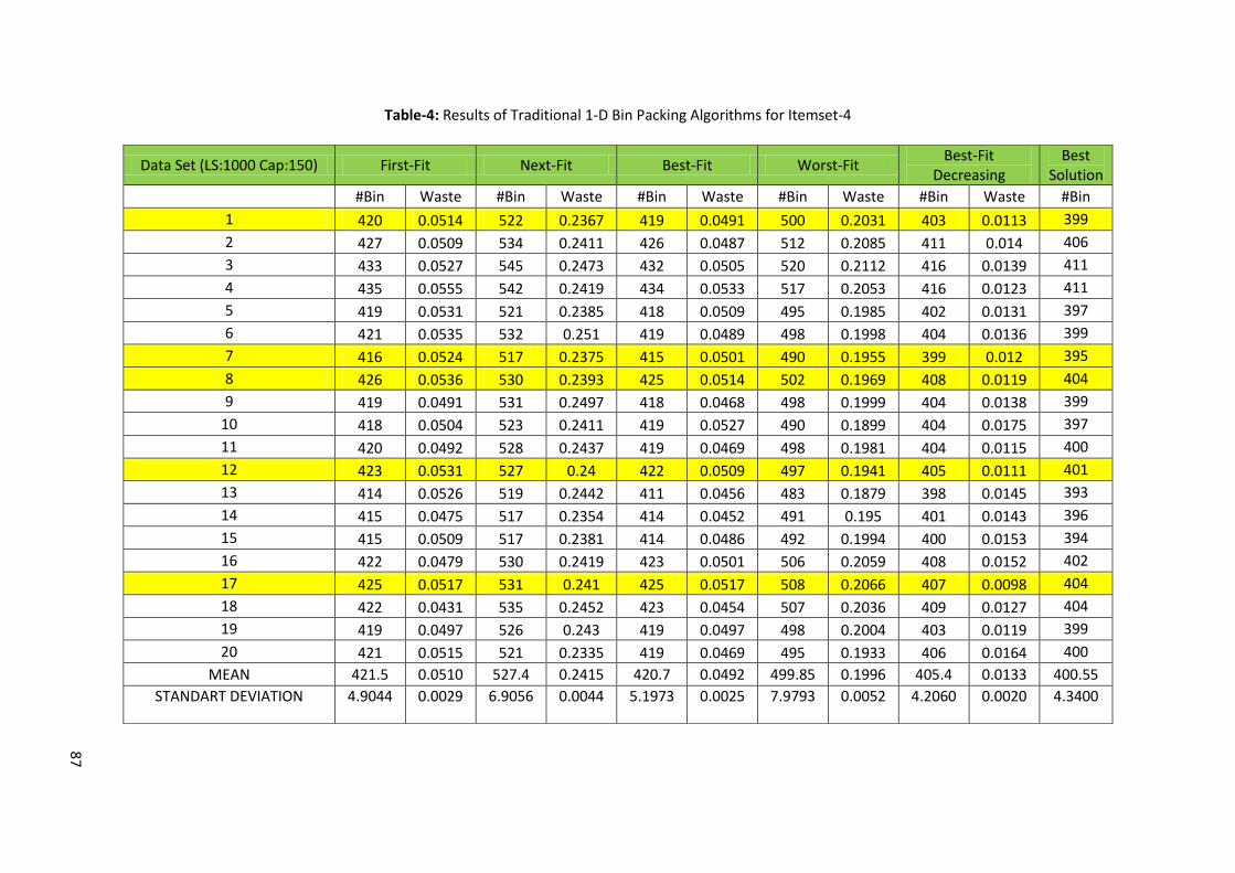
87

Table-4: Results of Traditional 1-D Bin Packing Algorithms for Itemset-4

Data Set (LS:1000 Cap:150) First-Fit Next-Fit Best-Fit Worst-Fit Best-Fit

Decreasing Best

Solution

#Bin Waste #Bin Waste #Bin Waste #Bin Waste #Bin Waste #Bin

1 420 0.0514 522 0.2367 419 0.0491 500 0.2031 403 0.0113 399

2 427 0.0509 534 0.2411 426 0.0487 512 0.2085 411 0.014 406

3 433 0.0527 545 0.2473 432 0.0505 520 0.2112 416 0.0139 411

4 435 0.0555 542 0.2419 434 0.0533 517 0.2053 416 0.0123 411

5 419 0.0531 521 0.2385 418 0.0509 495 0.1985 402 0.0131 397

6 421 0.0535 532 0.251 419 0.0489 498 0.1998 404 0.0136 399

7 416 0.0524 517 0.2375 415 0.0501 490 0.1955 399 0.012 395

8 426 0.0536 530 0.2393 425 0.0514 502 0.1969 408 0.0119 404

9 419 0.0491 531 0.2497 418 0.0468 498 0.1999 404 0.0138 399

10 418 0.0504 523 0.2411 419 0.0527 490 0.1899 404 0.0175 397

11 420 0.0492 528 0.2437 419 0.0469 498 0.1981 404 0.0115 400

12 423 0.0531 527 0.24 422 0.0509 497 0.1941 405 0.0111 401

13 414 0.0526 519 0.2442 411 0.0456 483 0.1879 398 0.0145 393

14 415 0.0475 517 0.2354 414 0.0452 491 0.195 401 0.0143 396

15 415 0.0509 517 0.2381 414 0.0486 492 0.1994 400 0.0153 394

16 422 0.0479 530 0.2419 423 0.0501 506 0.2059 408 0.0152 402

17 425 0.0517 531 0.241 425 0.0517 508 0.2066 407 0.0098 404

18 422 0.0431 535 0.2452 423 0.0454 507 0.2036 409 0.0127 404

19 419 0.0497 526 0.243 419 0.0497 498 0.2004 403 0.0119 399

20 421 0.0515 521 0.2335 419 0.0469 495 0.1933 406 0.0164 400

MEAN 421.5 0.0510 527.4 0.2415 420.7 0.0492 499.85 0.1996 405.4 0.0133 400.55

STANDART DEVIATION 4.9044 0.0029 6.9056 0.0044 5.1973 0.0025 7.9793 0.0052 4.2060 0.0020 4.3400

88

Table-5: Results of Traditional 1-D Bin Packing Algorithms for Itemset-5

Data Set (LS:60 Cap:100) First-Fit Next-Fit Best-Fit Worst-Fit Best-Fit

Decreasing Best

Solution

#Bin Waste #Bin Waste #Bin Waste #Bin Waste #Bin Waste #Bin

1 22 0.0909 24 0.1667 22 0.0909 23 0.1304 23 0.1304 20

2 21 0.0476 21 0.0476 21 0.0476 21 0.0476 23 0.1304 20

3 22 0.0909 23 0.1304 22 0.0909 22 0.0909 23 0.1304 20

4 23 0.1304 25 0.2 23 0.1304 24 0.1667 23 0.1304 20

5 21 0.0476 25 0.2 21 0.0476 22 0.0909 24 0.1667 20

6 22 0.0909 24 0.1667 22 0.0909 23 0.1304 23 0.1304 20

7 22 0.0909 22 0.0909 22 0.0909 21 0.0476 23 0.1304 20

8 21 0.0476 23 0.1304 21 0.0476 22 0.0909 23 0.1304 20

9 22 0.0909 24 0.1667 22 0.0909 23 0.1304 23 0.1304 20

10 22 0.0909 24 0.1667 22 0.0909 23 0.1304 23 0.1304 20

11 22 0.0909 24 0.1667 22 0.0909 23 0.1304 23 0.1304 20

12 23 0.1304 25 0.2 23 0.1304 23 0.1304 24 0.1667 20

13 22 0.0909 22 0.0909 22 0.0909 21 0.0476 23 0.1304 20

14 22 0.0909 23 0.1304 22 0.0909 22 0.0909 23 0.1304 20

15 22 0.0909 24 0.1667 22 0.0909 23 0.1304 23 0.1304 20

16 22 0.0909 24 0.1667 22 0.0909 23 0.1304 23 0.1304 20

17 21 0.0476 23 0.1304 21 0.0476 22 0.0909 24 0.1667 20

18 22 0.0909 24 0.1667 22 0.0909 24 0.1667 24 0.1667 20

19 22 0.0909 24 0.1667 22 0.0909 23 0.1304 23 0.1304 20

20 22 0.0909 23 0.1304 22 0.0909 22 0.0909 23 0.1304 20

MEAN 21.9 0.0862 23.55 0.1491 21.9 0.0862 22.5 0.1098 23.2 0.1377 20

STANDART DEVIATION 0.5392 0.0225 0.8929 0.0324 0.5392 0.0225 0.8445 0.0336 0.4243 0.0154 0.0000

89

Table-6: Results of Traditional 1-D Bin Packing Algorithms for Itemset-6

Data Set (LS:120 Cap:100) First-Fit Next-Fit Best-Fit Worst-Fit Best-Fit

Decreasing Best

Solution

#Bin Waste #Bin Waste #Bin Waste #Bin Waste #Bin Waste #Bin

1 43 0.0698 47 0.1489 43 0.0698 46 0.1304 45 0.1111 40

2 43 0.0698 47 0.1489 43 0.0698 45 0.1111 45 0.1111 40

3 42 0.0476 47 0.1489 42 0.0476 44 0.0909 45 0.1111 40

4 44 0.0909 48 0.1667 44 0.0909 45 0.1111 46 0.1304 40

5 44 0.0909 47 0.1489 44 0.0909 45 0.1111 46 0.1304 40

6 44 0.0909 46 0.1304 44 0.0909 44 0.0909 46 0.1304 40

7 43 0.0698 46 0.1304 43 0.0698 44 0.0909 45 0.1111 40

8 43 0.0698 48 0.1667 43 0.0698 46 0.1304 46 0.1304 40

9 43 0.0698 48 0.1667 43 0.0698 45 0.1111 46 0.1304 40

10 43 0.0698 49 0.1837 43 0.0698 45 0.1111 45 0.1111 40

11 44 0.0909 48 0.1667 44 0.0909 46 0.1304 46 0.1304 40

12 43 0.0698 49 0.1837 43 0.0698 47 0.1489 46 0.1304 40

13 43 0.0698 47 0.1489 43 0.0698 45 0.1111 46 0.1304 40

14 44 0.0909 47 0.1489 43 0.0698 44 0.0909 46 0.1304 40

15 43 0.0698 46 0.1304 43 0.0698 43 0.0698 46 0.1304 40

16 44 0.0909 47 0.1489 44 0.0909 45 0.1111 46 0.1304 40

17 43 0.0698 46 0.1304 43 0.0698 45 0.1111 46 0.1304 40

18 43 0.0698 46 0.1304 43 0.0698 44 0.0909 47 0.1489 40

19 43 0.0698 45 0.1111 43 0.0698 44 0.0909 46 0.1304 40

20 44 0.0909 49 0.1837 44 0.0909 47 0.1489 46 0.1304 40

MEAN 43.3 0.0761 47.15 0.1512 43.25 0.0750 44.95 0.1097 45.8 0.1265 40

STANDART DEVIATION 0.4929 0.0104 1.1998 0.0216 0.4785 0.0101 1.0556 0.0207 0.4173 0.0079 0.0000

90

Table-7: Results of Traditional 1-D Bin Packing Algorithms for Itemset-7

Data Set (LS:249 Cap:100) First-Fit Next-Fit Best-Fit Worst-Fit Best-Fit

Decreasing Best

Solution

#Bin Waste #Bin Waste #Bin Waste #Bin Waste #Bin Waste #Bin

1 89 0.0674 98 0.1531 89 0.0674 93 0.1075 94 0.117 83

2 89 0.0674 98 0.1531 89 0.0674 93 0.1075 95 0.1263 83

3 88 0.0568 98 0.1531 88 0.0568 92 0.0978 94 0.117 83

4 89 0.0674 97 0.1443 89 0.0674 92 0.0978 95 0.1263 83

5 90 0.0778 98 0.1531 90 0.0778 93 0.1075 95 0.1263 83

6 89 0.0674 94 0.117 89 0.0674 91 0.0879 95 0.1263 83

7 91 0.0879 97 0.1443 91 0.0879 93 0.1075 95 0.1263 83

8 89 0.0674 100 0.17 89 0.0674 92 0.0978 96 0.1354 83

9 88 0.0568 98 0.1531 88 0.0568 92 0.0978 95 0.1263 83

10 88 0.0568 95 0.1263 88 0.0568 90 0.0778 95 0.1263 83

11 89 0.0674 100 0.17 89 0.0674 92 0.0978 95 0.1263 83

12 89 0.0674 97 0.1443 89 0.0674 92 0.0978 96 0.1354 83

13 88 0.0568 101 0.1782 89 0.0674 94 0.117 94 0.117 83

14 90 0.0778 99 0.1616 90 0.0778 92 0.0978 96 0.1354 83

15 89 0.0674 97 0.1443 89 0.0674 91 0.0879 95 0.1263 83

16 89 0.0674 99 0.1616 89 0.0674 93 0.1075 95 0.1263 83

17 90 0.0778 101 0.1782 90 0.0778 94 0.117 96 0.1354 83

18 89 0.0674 100 0.17 89 0.0674 93 0.1075 94 0.117 83

19 90 0.0778 99 0.1616 90 0.0778 94 0.117 94 0.117 83

20 90 0.0778 98 0.1531 90 0.0778 94 0.117 96 0.1354 83

MEAN 89.15 0.0689 98.2 0.1545 89.2 0.0694 92.5 0.1026 95 0.1263 83

STANDART DEVIATION 0.8068 0.0084 1.8952 0.0165 0.7490 0.0078 1.1437 0.0111 0.6764 0.0062 0.0000

91

Table-8: Results of Traditional 1-D Bin Packing Algorithms for Itemset-8

Data Set (LS:501 Cap:100) First-Fit Next-Fit Best-Fit Worst-Fit Best-Fit

Decreasing Best

Solution

#Bin Waste #Bin Waste #Bin Waste #Bin Waste #Bin Waste #Bin

1 178 0.0618 196 0.148 178 0.0618 184 0.0924 190 0.1211 167

2 181 0.0773 200 0.165 180 0.0722 186 0.1022 191 0.1257 167

3 178 0.0618 194 0.1392 178 0.0618 186 0.1022 190 0.1211 167

4 178 0.0618 196 0.148 178 0.0618 188 0.1117 191 0.1257 167

5 178 0.0618 194 0.1392 179 0.067 185 0.0973 191 0.1257 167

6 178 0.0618 194 0.1392 178 0.0618 182 0.0824 190 0.1211 167

7 178 0.0618 197 0.1523 178 0.0618 185 0.0973 190 0.1211 167

8 179 0.067 199 0.1608 179 0.067 187 0.107 189 0.1164 167

9 178 0.0618 199 0.1608 178 0.0618 190 0.1211 191 0.1257 167

10 178 0.0618 191 0.1257 178 0.0618 183 0.0874 190 0.1211 167

11 179 0.067 192 0.1302 179 0.067 184 0.0924 190 0.1211 167

12 177 0.0565 196 0.148 177 0.0565 184 0.0924 190 0.1211 167

13 179 0.067 204 0.1814 179 0.067 194 0.1392 190 0.1211 167

14 179 0.067 195 0.1436 179 0.067 183 0.0874 190 0.1211 167

15 180 0.0722 195 0.1436 179 0.067 184 0.0924 189 0.1164 167

16 180 0.0722 197 0.1523 179 0.067 186 0.1022 191 0.1257 167

17 178 0.0618 198 0.1566 178 0.0618 189 0.1164 189 0.1164 167

18 180 0.0722 200 0.165 179 0.067 187 0.107 191 0.1257 167

19 179 0.067 202 0.1733 179 0.067 186 0.1022 189 0.1164 167

20 178 0.0618 197 0.1523 178 0.0618 185 0.0973 191 0.1257 167

MEAN 178.65 0.0652 196.8 0.1512 178.5 0.0644 185.9 0.1015 190.15 0.1218 167

STANDART DEVIATION 0.8444 0.0044 3.2582 0.0140 0.6057 0.0032 2.9105 0.0138 0.7579 0.0035 0.0000

92

Appendix B

93

Table 9.A: Results of Classic ABC Algorithm for Itemset-1 Group-1

Fig. 1.A: Average Number of Bin for Table 9.A Fig. 1.B: Average Wastage for Table 9.A

Swarm:100 Iteration:7500 Max Number of Fail:100 Minimum Bin Usage Ratio:0.50 Group:1 Optimum Number of Bin:48

Test 1 2 3 4 5 OVERALL

Time(sc) 939.0273 936.5731 936.2996 935.5605 934.8444 BIN WASTE

Bin Waste Bin Waste Bin Waste Bin Waste Bin Waste Best No.Best Mean St.

Dev. Best No.Best Mean St.

Dev.

Best 49 0.037 48 0.0228 48 0.0226 48 0.0226 48 0.0222 48 4 48.2 0.4472 0.0222 1 0.0254 0.0065

Mean 49.038 0.0378 48.981 0.0372 48.949 0.0367 48.511 0.0326 48.962 0.0368 48.511 1 48.888 0.2137 0.0326 1 0.0362 0.0021

St. Dev. 0.3575 0.0067 0.4581 0.0079 0.4625 0.0079 0.6929 0.01 0.4721 0.0081 0.3575 1 0.4886 0.1233 0.0067 1 0.0081 0.0012

94

Table 9.B: Results of Classic ABC Algorithm for Itemset-1 Group-7

Swarm:100 Iteration:7500 Max Number of Fail:100 Minimum Bin Usage Ratio:0.50 Group:7 Optimum Number of Bin:48

Test 1 2 3 4 5 OVERALL

Time(sc) 997.6559 986.0989 975.8165 981.1598 985.1547 BIN WASTE

Bin Waste Bin Waste Bin Waste Bin Waste Bin Waste Best No.Best Mean St.

Dev. Best No.Best Mean St.

Dev.

Best 49 0.029 49 0.029 49 0.029 49 0.029 49 0.029 49 5 49 0.0000 0.0290 5 0.0290 0.0000

Mean 49.047 0.0301 49.049 0.0303 49.038 0.0298 49.037 0.0301 49.046 0.0298 49.037 1 49.043 0.0057 0.0298 2 0.0300 0.0002

St. Dev. 0.4161 0.0079 0.3926 0.0075 0.3905 0.0073 0.3926 0.0075 0.3926 0.0075 0.3905 1 0.3969 0.0108 0.0073 1 0.0075 0.0002

Fig. 2.A: Average Number of Bin for Table 9.B Fig. 2.B: Average Wastage for Table 9.B

95

Table 9.C: Results of Classic ABC Algorithm for Itemset-1 Group-8

Swarm:100 Iteration:7500 Max Number of Fail:100 Minimum Bin Usage Ratio:0.50 Group:8 Optimum Number of Bin:49

Test 1 2 3 4 5 OVERALL

Time(sc) 1.01E+03 9.91E+02 9.76E+02 9.68E+02 9.86E+02 BIN WASTE

Bin Waste Bin Waste Bin Waste Bin Waste Bin Waste Best No.Best Mean St.

Dev. Best No.Best Mean St.

Dev.

Best 50 0.0273 50 0.0273 50 0.0273 50 0.0273 50 0.0273 50 5 50 0.0000 0.0273 5 0.0273 0.0000

Mean 50.056 0.0295 50.044 0.0285 50.043 0.029 50.044 0.0285 50.056 0.0295 50.043 1 50.048 0.0066 0.0285 2 0.0290 0.0005

St. Dev. 0.3756 0.0071 0.3523 0.0066 0.365 0.007 0.3523 0.0066 0.3756 0.0071 0.3523 2 0.3642 0.0117 0.0066 2 0.0069 0.0003

Fig. 3.A: Average Number of Bin for Table 9.C Fig. 3.B: Average Wastage for Table 9.C

96

Table 9.D: Results of Classic ABC Algorithm for Itemset-1 Group-12

Fig. 4.A: Average Number of Bin for Table 9.D Fig. 4.B: Average Wastage for Table 9.D

Swarm:100 Iteration:7500 Max Number of Fail:100 Minimum Bin Usage Ratio:0.50 Group:12 Optimum Number of Bin:49

Test 1 2 3 4 5 OVERALL

Time(sc) 965.2107 959.0011 950.5929 978.3648 954.8614 BIN WASTE

Bin Waste Bin Waste Bin Waste Bin Waste Bin Waste Best No.Best Mean St.

Dev. Best No.Best Mean St.

Dev.

Best 50 0.0337 50 0.0337 50 0.0337 50 0.0337 50 0.0337 50 5 50 0.0000 0.0337 5 0.0337 0.0000

Mean 50.050 0.0348 50.060 0.0349 50.062 0.0351 50.050 0.0350 50.050 0.0348 50.050 3 50.054 0.0058 0.0348 2 0.0349 0.0001

St. Dev. 0.4140 0.0078 0.4791 0.0086 0.4693 0.0084 0.4140 0.0078 0.4140 0.0078 0.4140 3 0.4381 0.0332 0.0078 3 0.0081 0.0004

97

Table 9.E: Results of Classic ABC Algorithm for Itemset-1 Group-17

Fig. 5.A: Average Number of Bin for Table 9.E Fig. 5.B: Average Wastage for Table 9.E

Swarm:100 Iteration:7500 Max Number of Fail:100 Minimum Bin Usage Ratio:0.50 Group:17 Optimum Number of Bin:52

Test 1 2 3 4 5 OVERALL

Time(sc) 999.6798 988.5619 976.8857 971.2657 994.3791 BIN WASTE

Bin Waste Bin Waste Bin Waste Bin Waste Bin Waste Best No.Best Mean St.

Dev. Best No.Best Mean St.

Dev.

Best 53 0.0330 53 0.0330 52 0.0187 53 0.0330 53 0.0330 52 1 52.8 0.4472 0.0187 1 0.0301 0.0064

Mean 53.048 0.0339 53.061 0.0341 52.969 0.0330 53.058 0.0336 53.048 0.0339 52.969 1 53.037 0.0382 0.0330 1 0.0337 0.0004

St. Dev. 0.4690 0.0080 0.5025 0.0085 0.5824 0.0091 0.5025 0.0085 0.4690 0.0080 0.4690 2 0.5051 0.0464 0.0080 2 0.0084 0.0005

98

Table 10.A: Results of Classic ABC Algorithm for Itemset-2 Group-5

Fig. 6.A: Average Number of Bin for Table 10.A Fig. 6.B: Average Wastage for Table 10.A

Swarm:100 Iteration:7500 Max Number of Fail:100 Minimum Bin Usage Ratio:0.50 Group:5 Optimum Number of Bin:101

Test 1 2 3 4 5 OVERALL

Time(sc) 2.20E+03 2.20E+03 2.15E+03 2.27E+03 2.13E+03 BIN WASTE

Bin Waste Bin Waste Bin Waste Bin Waste Bin Waste Best No.Best Mean St.

Dev. Best No.Best Mean St.

Dev.

Best 103 0.0256 103 0.0249 103 0.0256 103 0.0256 103 0.0256 103 5 103 0.0000 0.0249 1 0.0255 0.0003

Mean 103.35 0.0329 103.33 0.0327 103.35 0.0329 103.35 0.0329 103.35 0.0329 103.33 1 103.35 0.0089 0.0327 1 0.0329 0.0001

St. Dev. 0.5416 0.0053 0.4136 0.0041 0.5416 0.0053 0.5416 0.0053 0.5416 0.0053 0.4136 1 0.5160 0.0572 0.0041 1 0.0051 0.0005

99

Table 10.B: Results of Classic ABC Algorithm for Itemset-2 Group-6

Fig. 7.A: Average Number of Bin for Table 10.B Fig. 7.B: Average Wastage for Table 10.B

Swarm:100 Iteration:7500 Max Number of Fail:100 Minimum Bin Usage Ratio:0.50 Group:6 Optimum Number of Bin:101

Test 1 2 3 4 5 OVERALL

Time(sc) 2.21E+03 2.34E+03 2.13E+03 2.15E+03 2.29E+03 BIN WASTE

Bin Waste Bin Waste Bin Waste Bin Waste Bin Waste Best No.Best Mean St.

Dev. Best No.Best Mean St.

Dev.

Best 104 0.0305 104 0.0305 104 0.0305 104 0.0305 104 0.0305 104 5 104 0.0000 0.0305 5 0.0305 0.0000

Mean 104.39 0.0341 104.33 0.0336 104.36 0.0341 104.38 0.0321 104.37 0.0345 104.327 1 104.364 0.0244 0.0321 1 0.0337 0.0009

St. Dev. 1.5112 0.0128 1.4908 0.0126 1.5112 0.0128 1.5112 0.0128 1.5112 0.0128 1.4908 1 1.5071 0.0091 0.0126 1 0.0128 0.0001

100

Table 10.C: Results of Classic ABC Algorithm for Itemset-2 Group-14

Fig. 8.A: Average Number of Bin for Table 10.B Fig. 8.B: Average Wastage for Table 10.B

Swarm:100 Iteration:7500 Max Number of Fail:100 Minimum Bin Usage Ratio:0.50 Group:14 Optimum Number of Bin:103

Test 1 2 3 4 5 OVERALL

Time(sc) 2.15E+03 2.35E+03 2.17E+03 2.13E+03 2.25E+03 BIN WASTE

Bin Waste Bin Waste Bin Waste Bin Waste Bin Waste Best No.Best Mean St.

Dev. Best No.Best Mean St.

Dev.

Best 105 0.029 105 0.029 105 0.029 105 0.029 105 0.029 105 5 105 0.0000 0.0290 5 0.0290 0.0000

Mean 105.44 0.0334 105.69 0.0358 105.54 0.0355 105.62 0.0349 105.69 0.0358 105.440 1 105.598 0.1077 0.0334 1 0.0351 0.0010

St. Dev. 1.5267 0.0127 1.4459 0.012 1.4459 0.012 1.4459 0.012 1.4459 0.012 1.4459 4 1.4621 0.0361 0.0120 4 0.0121 0.0003

101

Table 10.D: Results of Classic ABC Algorithm for Itemset-2 Group-16

Fig. 9.A: Average Number of Bin for Table 10.D Fig. 9.B: Average Wastage for Table 10.D

Swarm:100 Iteration:7500 Max Number of Fail:100 Minimum Bin Usage Ratio:0.50 Group:16 Optimum Number of Bin:105

Test 1 2 3 4 5 OVERALL

Time(sc) 2.12E+03 2.12E+03 2.32E+03 2.15E+03 2.13E+03 BIN WASTE

Bin Waste Bin Waste Bin Waste Bin Waste Bin Waste Best No.Best Mean St.

Dev. Best No.Best Mean St.

Dev.

Best 108 0.0295 108 0.0295 108 0.0295 108 0.0295 108 0.0295 108 5 108 0.0000 0.0295 5 0.0295 0.0000

Mean 108.31 0.0323 108.34 0.0326 108.31 0.0323 108.33 0.0326 108.32 0.0326 108.306 2 108.321 0.0163 0.0323 2 0.0325 0.0002

St. Dev. 1.6077 0.0131 1.7157 0.0138 1.6077 0.0131 1.7157 0.0138 1.7157 0.0138 1.6077 2 1.6725 0.0591 0.0131 2 0.0135 0.0004

102

Table 10.E: Results of Classic ABC Algorithm for Itemset-2 Group-19

Fig. 10.A: Average Number of Bin for Table 10.E Fig. 10.B: Average Wastage for Table 10.E

Swarm:100 Iteration:7500 Max Number of Fail:100 Minimum Bin Usage Ratio:0.50 Group:19 Optimum Number of Bin:100

Test 1 2 3 4 5 OVERALL

Time(sc) 2.40E+03 2.40E+03 2.40E+03 2.39E+03 2.40E+03 BIN WASTE

Bin Waste Bin Waste Bin Waste Bin Waste Bin Waste Best No.Best Mean St.

Dev. Best No.Best Mean St.

Dev.

Best 102 0.0239 102 0.0244 102 0.0239 102 0.0241 102 0.0244 102 5 102 0.0000 0.0239 2 0.0241 0.0003

Mean 103.14 0.0337 102.95 0.0324 103.14 0.0337 102.95 0.0345 102.95 0.0324 102.949 2 103.025 0.1034 0.0324 2 0.0333 0.0009

St. Dev. 1.4668 0.0127 0.7272 0.0067 1.4668 0.0127 0.7285 0.0087 0.7272 0.0067 0.7272 2 1.0233 0.4049 0.0067 2 0.0095 0.0030

103

Table 11: Results of Classic ABC Algorithm and MEABC Algorithm for Itemset-3

Fig. 11.A: ABC Results for Number of Bin for Group-3 in Table 11 Fig. 11.B: ABC Results for Wastage for Group-3 in Table 11

104

Fig. 12.A: ABC Results for Number of Bin for Group-10 in Table 11 Fig. 12.B: ABC Results for Wastage for Group-10 in Table 11

Fig. 13.A: ABC Results for Number of Bin for Group-11 in Table 11 Fig. 13.B: ABC Results for Wastage for Group-11 in Table 11

105

Fig. 14.A: ABC Results for Number of Bin for Group-13 in Table 11 Fig. 14.B: ABC Results for Wastage for Group-13 in Table 11

Fig. 15.A: ABC Results for Number of Bin for Group-20 in Table 11 Fig. 15.B: ABC Results for Wastage for Group-20 in Table 11

106

Table 12: Results of Classic ABC Algorithm and MEABC Algorithm for Itemset-4

Fig. 16.A: ABC Results for Number of Bin for Group-1 in Table 12 Fig. 16.B: ABC Results for Wastage for Group-1 in Table 12

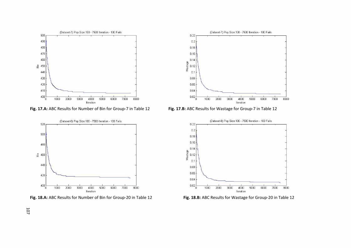
107

Fig. 17.A: ABC Results for Number of Bin for Group-7 in Table 12 Fig. 17.B: ABC Results for Wastage for Group-7 in Table 12

Fig. 18.A: ABC Results for Number of Bin for Group-20 in Table 12 Fig. 18.B: ABC Results for Wastage for Group-20 in Table 12

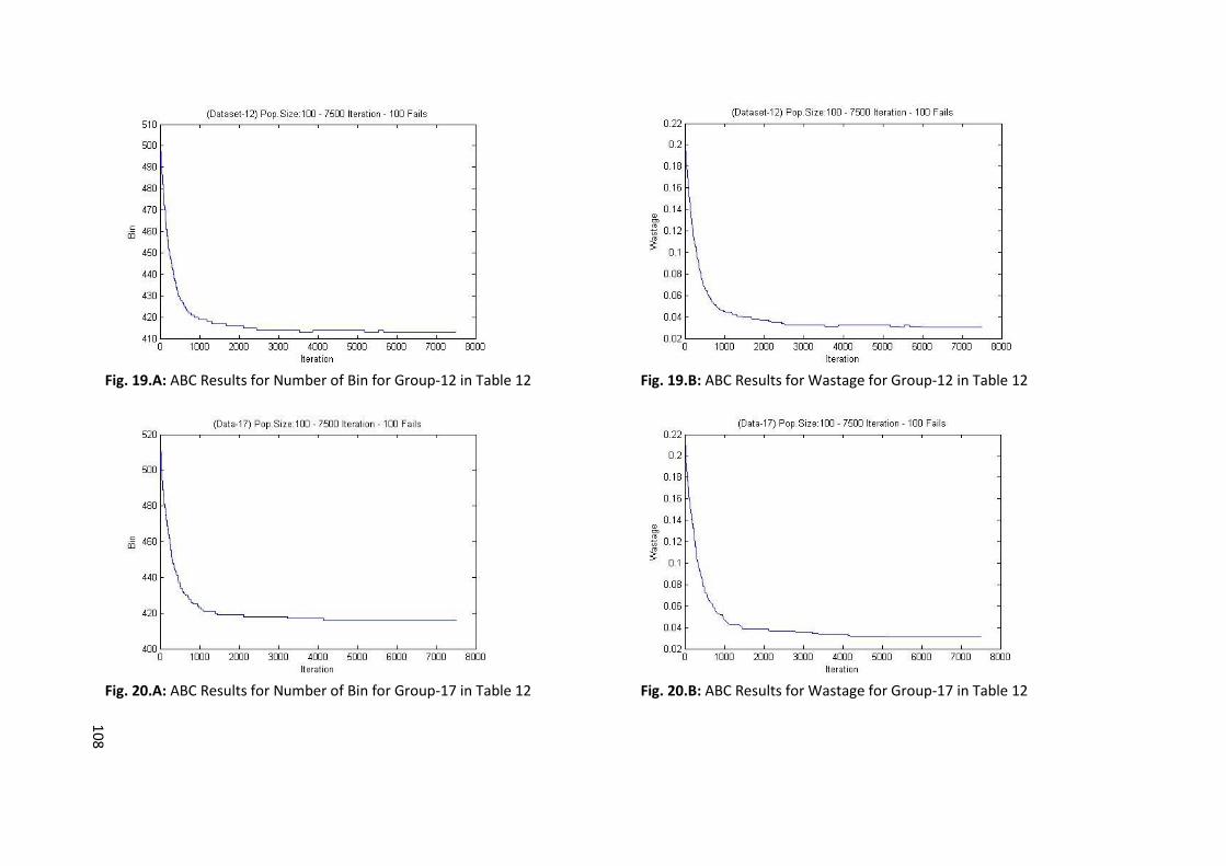
108

Fig. 19.A: ABC Results for Number of Bin for Group-12 in Table 12 Fig. 19.B: ABC Results for Wastage for Group-12 in Table 12

Fig. 20.A: ABC Results for Number of Bin for Group-17 in Table 12 Fig. 20.B: ABC Results for Wastage for Group-17 in Table 12

109

Table 13.A: Results of Classic ABC Algorithm for Itemset-5 Group-2

Fig. 21.A: Average Number of Bin for Table 13.A Fig. 21.B: Average Wastage for Table 13.A

Swarm:100 Iteration:7500 Max Number of Fail:100 Minimum Bin Usage Ratio:0.50 Group:2 Optimum Number of Bin:20

Test 1 2 3 4 5 OVERALL

Time(sc) 457.2261 462.4832 461.3166 469.2675 472.8706 BIN WASTE

Bin Waste Bin Waste Bin Waste Bin Waste Bin Waste Best No.Best Mean St.

Dev. Best No.Best Mean St.

Dev.

Best 21 0.0476 21 0.0476 21 0.0476 20 0.0198 21 0.0476 20 1 20.8 0.4472 0.0198 1 0.0420 0.0124

Mean 21.001 0.0478 21.002 0.0478 21.002 0.0478 20.989 0.0474 21.002 0.0478 20.989 1 20.9993 0.0059 0.0474 1 0.0477 0.0002

St. Dev. 0.0462 0.0025 0.0541 0.0027 0.0541 0.0027 0.1286 0.0042 0.0516 0.0025 0.0462 1 0.0669 0.0346 0.0025 2 0.0029 0.0007

110

Table 13.B: Results of Classic ABC Algorithm for Itemset-5 Group-4

Fig. 22.A: Average Number of Bin for Table 13.B Fig. 22.B: Average Wastage for Table 13.B

Swarm:100 Iteration:7500 Max Number of Fail:100 Minimum Bin Usage Ratio:0.50 Group:4 Optimum Number of Bin:20

Test 1 2 3 4 5 OVERALL

Time(sc) 457.0659 457.346 471.6333 457.2749 454.2206 BIN WASTE

Bin Waste Bin Waste Bin Waste Bin Waste Bin Waste Best No.Best Mean St.

Dev. Best No.Best Mean St.

Dev.

Best 21 0.0476 21 0.0476 21 0.0476 20 0.0228 21 0.0476 20 1 20.8 0.4472 0.0228 1 0.0426 0.0111

Mean 21.002 0.0483 21.002 0.0481 21.001 0.0477 20.971 0.047 21.002 0.0477 20.9711 1 20.9956 0.0137 0.0470 1 0.0478 0.0005

St. Dev. 0.0529 0.0036 0.0476 0.0031 0.0462 0.0024 0.1872 0.0052 0.0462 0.0024 0.0462 2 0.0760 0.0622 0.0024 2 0.0033 0.0012

111

Table 13.C: Results of Classic ABC Algorithm for Itemset-5 Group-9

Fig. 23.A: Average Number of Bin for Table 13.C Fig. 23.B: Average Wastage for Table 13.C

Swarm:100 Iteration:7500 Max Number of Fail:100 Minimum Bin Usage Ratio:0.50 Group:9 Optimum Number of Bin:20

Test 1 2 3 4 5 OVERALL

Time(sc) 421.8013 422.6551 422.7184 422.4861 439.1366 BIN WASTE

Bin Waste Bin Waste Bin Waste Bin Waste Bin Waste Best No.Best Mean St.

Dev. Best No.Best Mean St.

Dev.

Best 20 0.0234 20 0.0227 21 0.0476 21 0.0476 21 0.0476 20 2 20.6 0.5477 0.0227 1 0.0378 0.0134

Mean 20.927 0.0459 20.991 0.0475 21.001 0.0477 21.002 0.0478 21.002 0.0478 20.9267 1 20.9844 0.0326 0.0459 1 0.0473 0.0008

St. Dev. 0.2683 0.0067 0.111 0.0035 0.0365 0.0018 0.0447 0.0024 0.0503 0.0024 0.0365 1 0.1022 0.0974 0.0018 1 0.0034 0.0020

112

Table 13.D: Results of Classic ABC Algorithm for Itemset-5 Group-15

Fig. 24.A: Average Number of Bin for Table 13.D Fig. 24.B: Average Wastage for Table 13.D

Swarm:100 Iteration:7500 Max Number of Fail:100 Minimum Bin Usage Ratio:0.50 Group:15 Optimum Number of Bin:20

Test 1 2 3 4 5 OVERALL

Time(sc) 479.7274 503.2211 499.5773 501.9112 504.3433 BIN WASTE

Bin Waste Bin Waste Bin Waste Bin Waste Bin Waste Best No.Best Mean St.

Dev. Best No.Best Mean St.

Dev.

Best 21 0.0476 20 0.0237 21 0.0476 20 0.0232 21 0.0476 20 2 20.6 0.5477 0.0232 1 0.0379 0.0132

Mean 21.002 0.0478 20.969 0.047 21.003 0.0478 20.981 0.0472 21.003 0.048 20.9685 1 20.9914 0.0158 0.0470 1 0.0476 0.0004

St. Dev. 0.0565 0.0028 0.1892 0.0051 0.0577 0.0029 0.1551 0.0044 0.06 0.0033 0.0565 1 0.1037 0.0637 0.0028 1 0.0037 0.0010

113

Table 13.E: Results of Classic ABC Algorithm for Itemset-5 Group-18

Fig. 25.A: Average Number of Bin for Table 13.E Fig. 25.B: Average Wastage for Table 13.E

Swarm:100 Iteration:7500 Max Number of Fail:100 Minimum Bin Usage Ratio:0.50 Group:18 Optimum Number of Bin:20

Test 1 2 3 4 5 OVERALL

Time(sc) 436.6198 437.2098 461.036 475.4929 474.1831 BIN WASTE

Bin Waste Bin Waste Bin Waste Bin Waste Bin Waste Best No.Best Mean St.

Dev. Best No.Best Mean St.

Dev.

Best 20 0.0234 21 0.0476 21 0.0476 21 0.0476 21 0.0476 20 1 20.8 0.4472 0.0234 1 0.0428 0.0108

Mean 20.946 0.0464 21.001 0.0478 21.003 0.0478 21.002 0.0478 21.003 0.0478 20.9457 1 20.9909 0.0253 0.0464 1 0.0475 0.0006

St. Dev. 0.2397 0.0063 0.04 0.0024 0.0588 0.0028 0.0577 0.0027 0.0653 0.0031 0.0400 1 0.0923 0.0829 0.0024 1 0.0035 0.0016

114

Table 14.A: Results of Classic ABC Algorithm for Itemset-6 Group-2

Swarm:100 Iteration:7500 Max Number of Fail:100 Minimum Bin Usage Ratio:0.50 Group:2 Optimum Number of Bin:40

Test 1 2 3 4 5 OVERALL

Time(sc) 916.9337 917.1444 912.4433 910.5781 919.3476 BIN WASTE

Bin Waste Bin Waste Bin Waste Bin Waste Bin Waste Best No.Best Mean St.

Dev. Best No.Best Mean St.

Dev.

Best 42 0.0476 42 0.0476 41 0.0348 42 0.0476 42 0.0476 41 1 41.8 0.4472 0.0348 1 0.0451 0.0057

Mean 42.016 0.0481 42.011 0.0479 42.005 0.0479 42.011 0.0479 42.016 0.0481 42.005 1 42.012 0.0045 0.0479 1 0.0480 0.0001

St. Dev. 0.2123 0.0048 0.1808 0.0040 0.2122 0.0045 0.1808 0.0040 0.2123 0.0048 0.1808 2 0.1997 0.0172 0.0040 2 0.0044 0.0004

Fig. 26.A: Average Number of Bin for Table 14.A Fig. 26.B: Average Wastage for Table 14.A

115

Table 14.B: Results of Classic ABC Algorithm for Itemset-6 Group-3

Fig. 27.A: Average Number of Bin for Table 14.B Fig. 27.B: Average Wastage for Table 14.B

Swarm:100 Iteration:7500 Max Number of Fail:100 Minimum Bin Usage Ratio:0.50 Group:3 Optimum Number of Bin:40

Test 1 2 3 4 5 OVERALL

Time(sc) 919.4462 919.9926 941.0009 935.6478 925.2179 BIN WASTE

Bin Waste Bin Waste Bin Waste Bin Waste Bin Waste Best No.Best Mean St.

Dev. Best No.Best Mean St.

Dev.

Best 42 0.0476 42 0.0476 42 0.0476 42 0.0476 42 0.0476 42 5 42 0.0000 0.0476 1 0.0476 0.0000

Mean 42.014 0.0482 42.022 0.0485 42.014 0.0480 42.037 0.0494 42.014 0.0482 42.014 2 42.020 0.0102 0.0480 1 0.0484 0.0006

St. Dev. 0.2019 0.0046 0.2210 0.0052 0.1864 0.0042 0.2596 0.0060 0.2019 0.0046 0.1864 1 0.2142 0.0282 0.0042 1 0.0049 0.0007

116

Table 14.C: Results of Classic ABC Algorithm for Itemset-6 Group-5

Swarm:100 Iteration:7500 Max Number of Fail:100 Minimum Bin Usage Ratio:0.50 Group:5 Optimum Number of Bin:40

Test 1 2 3 4 5 OVERALL

Time(sc) 931.7264 925.5368 919.1782 919.4462 935.6478 BIN WASTE

Bin Waste Bin Waste Bin Waste Bin Waste Bin Waste Best No.Best Mean St.

Dev. Best No.Best Mean St.

Dev.

Best 42 0.0537 42 0.0537 42 0.0476 42 0.0476 42 0.0476 42 5 42 0.0000 0.0476 1 0.0500 0.0033

Mean 42.857 0.0677 42.774 0.0667 42.013 0.0480 42.011 0.0479 42.014 0.0482 42.011 1 42.334 0.4408 0.0479 1 0.0557 0.0105

St. Dev. 0.3816 0.0061 0.4474 0.0067 0.1868 0.0043 0.1808 0.0040 0.2019 0.0046 0.1808 1 0.2797 0.1255 0.0040 1 0.0052 0.0012

Fig. 28.A: Average Number of Bin for Table 14.C Fig. 28.B: Average Wastage for Table 14.C

117

Table 14.D: Results of Classic ABC Algorithm for Itemset-6 Group-14

Fig. 29.A: Average Number of Bin for Table 14.D Fig. 29.B: Average Wastage for Table 14.D

Swarm:100 Iteration:7500 Max Number of Fail:100 Minimum Bin Usage Ratio:0.50 Group:14 Optimum Number of Bin:40

Test 1 2 3 4 5 OVERALL

Time(sc) 1.01E+03 1.03E+03 993.7954 1.03E+03 925.5368 BIN WASTE

Bin Waste Bin Waste Bin Waste Bin Waste Bin Waste Best No.Best Mean St.

Dev. Best No.Best Mean St.

Dev.

Best 41 0.0335 41 0.0341 42 0.0536 42 0.0537 42 0.0476 41 2 41.6 0.5477 0.0335 1 0.0445 0.0100

Mean 41.990 0.0476 41.998 0.0480 42.804 0.0670 42.857 0.0677 42.016 0.0481 41.990 1 42.333 0.4546 0.0476 1 0.0557 0.0107

St. Dev. 0.2398 0.0046 0.2110 0.0044 0.4199 0.0064 0.3816 0.0061 0.2123 0.0048 0.2110 1 0.2929 0.1000 0.0044 1 0.0052 0.0009

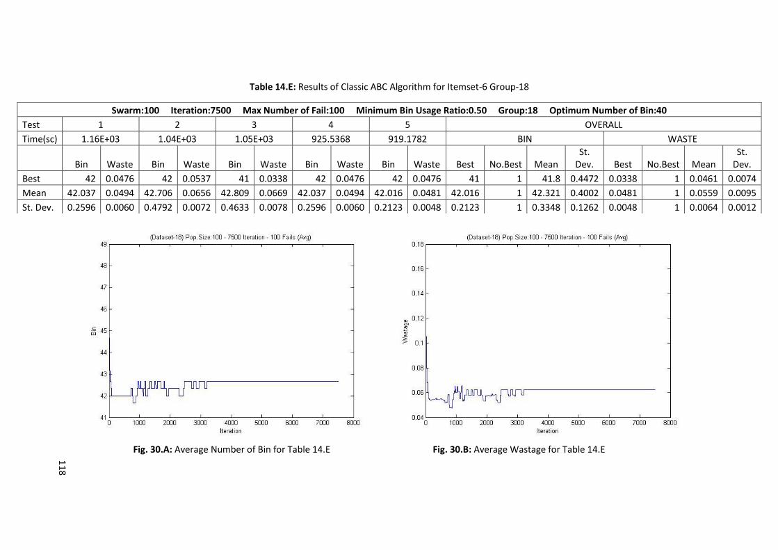
118

Table 14.E: Results of Classic ABC Algorithm for Itemset-6 Group-18

Fig. 30.A: Average Number of Bin for Table 14.E Fig. 30.B: Average Wastage for Table 14.E

Swarm:100 Iteration:7500 Max Number of Fail:100 Minimum Bin Usage Ratio:0.50 Group:18 Optimum Number of Bin:40

Test 1 2 3 4 5 OVERALL

Time(sc) 1.16E+03 1.04E+03 1.05E+03 925.5368 919.1782 BIN WASTE

Bin Waste Bin Waste Bin Waste Bin Waste Bin Waste Best No.Best Mean St.

Dev. Best No.Best Mean St.

Dev.

Best 42 0.0476 42 0.0537 41 0.0338 42 0.0476 42 0.0476 41 1 41.8 0.4472 0.0338 1 0.0461 0.0074

Mean 42.037 0.0494 42.706 0.0656 42.809 0.0669 42.037 0.0494 42.016 0.0481 42.016 1 42.321 0.4002 0.0481 1 0.0559 0.0095

St. Dev. 0.2596 0.0060 0.4792 0.0072 0.4633 0.0078 0.2596 0.0060 0.2123 0.0048 0.2123 1 0.3348 0.1262 0.0048 1 0.0064 0.0012

11

9

Table 15.A: Results of Classic ABC Algorithm for Itemset-7 Group-1

Fig. 31.A: Average Number of Bin for Table 15.A Fig. 31.B: Average Wastage for Table 15.A

Swarm:100 Iteration:7500 Max Number of Fail:100 Minimum Bin Usage Ratio:0.50 Group:1 Optimum Number of Bin:83

Test 1 2 3 4 5 OVERALL

Time(sc) 2.11E+03 2.07E+03 2.11E+03 2.12E+03 2.09E+03 BIN WASTE

Bin Waste Bin Waste Bin Waste Bin Waste Bin Waste Best No.Best Mean St.

Dev. Best No.Best Mean St.

Dev.

Best 87 0.0500 87 0.0494 87 0.0500 87 0.0500 87 0.0500 87 5 87 0.0000 0.0494 1 0.0498 0.0003

Mean 88.030 0.0574 88.039 0.0576 88.029 0.0574 88.030 0.0574 88.029 0.0574 88.029 1 88.031 0.0042 0.0574 4 0.0574 0.0001

St. Dev. 0.6641 0.0065 0.6033 0.0061 0.6548 0.0048 0.6247 0.0042 0.6643 0.0059 0.6033 1 0.6422 0.0271 0.0042 1 0.0055 0.0010

120

Table 15.B: Results of Classic ABC Algorithm for Itemset-7 Group-4

Fig. 32.A: Average Number of Bin for Table 15.B Fig. 32.B: Average Wastage for Table 15.B

Swarm:100 Iteration:7500 Max Number of Fail:100 Minimum Bin Usage Ratio:0.50 Group:4 Optimum Number of Bin:83

Test 1 2 3 4 5 OVERALL

Time(sc) 2.02E+03 2.02E+03 2.02E+03 2.01E+03 2.16E+03 BIN WASTE

Bin Waste Bin Waste Bin Waste Bin Waste Bin Waste Best No.Best Mean St.

Dev. Best No.Best Mean St.

Dev.

Best 87 0.0493 87 0.0507 87 0.0503 87 0.0526 87 0.0507 87 5 87 0.0000 0.0493 1 0.0507 0.0012

Mean 88.008 0.0572 88.848 0.0664 88.848 0.0652 88.184 0.0628 88.258 0.0662 88.008 1 88.429 0.3931 0.0572 1 0.0636 0.0038

St. Dev. 0.6262 0.0061 0.6915 0.0062 0.7426 0.0051 0.6471 0.0058 0.6572 0.0061 0.6262 1 0.6729 0.0455 0.0051 1 0.0059 0.0005

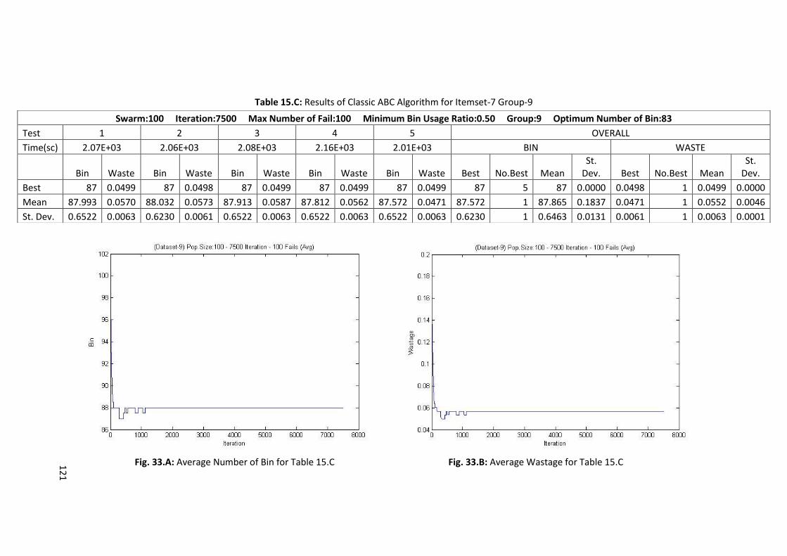
121

Table 15.C: Results of Classic ABC Algorithm for Itemset-7 Group-9

Fig. 33.A: Average Number of Bin for Table 15.C Fig. 33.B: Average Wastage for Table 15.C

Swarm:100 Iteration:7500 Max Number of Fail:100 Minimum Bin Usage Ratio:0.50 Group:9 Optimum Number of Bin:83

Test 1 2 3 4 5 OVERALL

Time(sc) 2.07E+03 2.06E+03 2.08E+03 2.16E+03 2.01E+03 BIN WASTE

Bin Waste Bin Waste Bin Waste Bin Waste Bin Waste Best No.Best Mean St.

Dev. Best No.Best Mean St.

Dev.

Best 87 0.0499 87 0.0498 87 0.0499 87 0.0499 87 0.0499 87 5 87 0.0000 0.0498 1 0.0499 0.0000

Mean 87.993 0.0570 88.032 0.0573 87.913 0.0587 87.812 0.0562 87.572 0.0471 87.572 1 87.865 0.1837 0.0471 1 0.0552 0.0046

St. Dev. 0.6522 0.0063 0.6230 0.0061 0.6522 0.0063 0.6522 0.0063 0.6522 0.0063 0.6230 1 0.6463 0.0131 0.0061 1 0.0063 0.0001

122

Table 15.D: Results of Classic ABC Algorithm for Itemset-7 Group-11

Fig. 34.A: Average Number of Bin for Table 15.D Fig. 34.B: Average Wastage for Table 15.D

Swarm:100 Iteration:7500 Max Number of Fail:100 Minimum Bin Usage Ratio:0.50 Group:11 Optimum Number of Bin:83

Test 1 2 3 4 5 OVERALL

Time(sc) 2.11E+03 2.02E+03 2.06E+03 2.09E+03 2.14E+03 BIN WASTE

Bin Waste Bin Waste Bin Waste Bin Waste Bin Waste Best No.Best Mean St.

Dev. Best No.Best Mean St.

Dev.

Best 87 0.0492 88 0.0568 88 0.0571 88 0.0531 88 0.0509 87 1 87.8 0.4472 0.0492 1 0.0534 0.0035

Mean 88.027 0.0573 88.059 0.0575 88.05 0.0585 88.058 0.0579 88.057 0.0581 88.027 1 88.050 0.0136 0.0573 1 0.0578 0.0005

St. Dev. 0.6528 0.0064 0.6222 0.0063 0.6222 0.0063 0.6792 0.0070 0.6542 0.0060 0.6222 2 0.6461 0.0242 0.0060 1 0.0064 0.0004

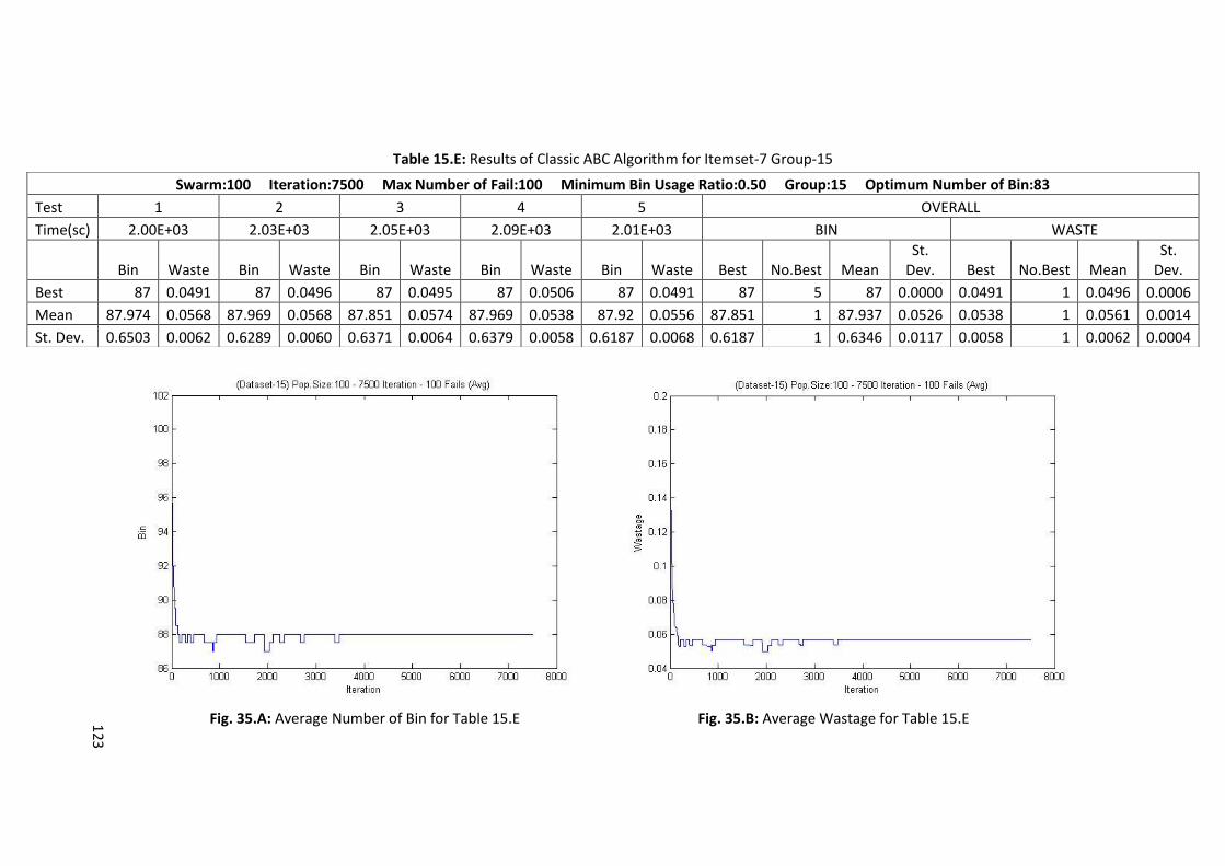
123

Table 15.E: Results of Classic ABC Algorithm for Itemset-7 Group-15

Fig. 35.A: Average Number of Bin for Table 15.E Fig. 35.B: Average Wastage for Table 15.E

Swarm:100 Iteration:7500 Max Number of Fail:100 Minimum Bin Usage Ratio:0.50 Group:15 Optimum Number of Bin:83

Test 1 2 3 4 5 OVERALL

Time(sc) 2.00E+03 2.03E+03 2.05E+03 2.09E+03 2.01E+03 BIN WASTE

Bin Waste Bin Waste Bin Waste Bin Waste Bin Waste Best No.Best Mean St.

Dev. Best No.Best Mean St.

Dev.

Best 87 0.0491 87 0.0496 87 0.0495 87 0.0506 87 0.0491 87 5 87 0.0000 0.0491 1 0.0496 0.0006

Mean 87.974 0.0568 87.969 0.0568 87.851 0.0574 87.969 0.0538 87.92 0.0556 87.851 1 87.937 0.0526 0.0538 1 0.0561 0.0014

St. Dev. 0.6503 0.0062 0.6289 0.0060 0.6371 0.0064 0.6379 0.0058 0.6187 0.0068 0.6187 1 0.6346 0.0117 0.0058 1 0.0062 0.0004

124

Table 16: Results of Classic ABC Algorithm and MEABC Algorithm for Itemset-8

Fig. 36.A: ABC Results for Number of Bin for Group-8 in Table 16 Fig. 36.B: ABC Results for Wastage for Group-8 in Table 16

125

Fig. 37.A: ABC Results for Number of Bin for Group-10 in Table 16 Fig. 37.B: ABC Results for Wastage for Group-10 in Table 16

Fig. 38.A: ABC Results for Number of Bin for Group-13 in Table 16 Fig. 38.B: ABC Results for Wastage for Group-13 in Table 16

126

Fig. 39.A: ABC Results for Number of Bin for Group-16 in Table 16 Fig. 39.B: ABC Results for Wastage for Group-16 in Table 16

Fig. 40.A: ABC Results for Number of Bin for Group-19 in Table 16 Fig. 40.B: ABC Results for Wastage for Group-19 in Table 16

127

Appendix C

128

Table-17.A: Results of MEABC Algorithm for Itemset-1 Group-1

Fig. 41.A: Average Number of Bin for Table 17.A Fig. 41.B: Average Wastage for Table 17.A

Swarm:100 Iteration:7500 Max Number of Fail:100 Tabu Period:1500 Minimum Bin Usage Ratio:0.50 Group:1 Optimum Number of Bin:48

Test 1 2 3 4 5 OVERALL

Time(sc) 958.1862 957.146 965.2645 954.3279 975.3468 BIN WASTE

Bin Waste Bin Waste Bin Waste Bin Waste Bin Waste Best No.Best Mean St.

Dev. Best No.Best Mean St.

Dev.

Best 48 0.0226 48 0.0228 49 0.037 48 0.0229 48 0.0228 48 4 48.2 0.4472 0.0226 1 0.0256 0.0064

Mean 48.946 0.0366 48.987 0.0372 49.038 0.0379 48.946 0.0369 48.987 0.0372 48.946 1 48.981 0.0381 0.0366 1 0.0372 0.0005

St. Dev. 0.4886 0.0083 0.4639 0.008 0.3392 0.0064 0.4886 0.0083 0.4639 0.008 0.3392 1 0.4488 0.0625 0.0064 1 0.0078 0.0008

129

Table-17.B: Results of MEABC Algorithm for Itemset-1 Group-7

Fig. 42.A: Average Number of Bin for Table 17.B Fig. 42.B: Average Wastage for Table 17.B

Swarm:100 Iteration:7500 Max Number of Fail:100 Tabu Period:1500 Minimum Bin Usage Ratio:0.50 Group:7 Optimum Number of Bin:48

Test 1 2 3 4 5 OVERALL

Time(sc) 936.2807 940.6256 972.808 968.3975 955.5571 BIN WASTE

Bin Waste Bin Waste Bin Waste Bin Waste Bin Waste Best No.Best Mean St.

Dev. Best No.Best Mean St.

Dev.

Best 49 0.029 49 0.029 49 0.029 49 0.029 49 0.029 49 5 49 0.0000 0.0290 5 0.0290 0.0000

Mean 49.058 0.0302 49.054 0.0303 49.04 0.0298 49.058 0.0301 49.054 0.0308 49.040 1 49.053 0.0075 0.0298 1 0.0302 0.0004

St. Dev. 0.4355 0.0081 0.4078 0.0077 0.3795 0.0071 0.4355 0.0081 0.4078 0.0077 0.3795 1 0.4132 0.0234 0.0071 1 0.0077 0.0004

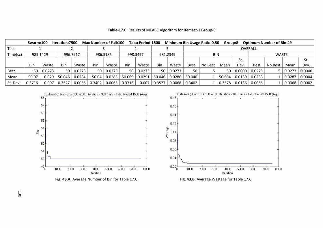
130

Table-17.C: Results of MEABC Algorithm for Itemset-1 Group-8

Swarm:100 Iteration:7500 Max Number of Fail:100 Tabu Period:1500 Minimum Bin Usage Ratio:0.50 Group:8 Optimum Number of Bin:49

Test 1 2 3 4 5 OVERALL

Time(sc) 985.1429 996.7917 986.5185 998.3497 981.2349 BIN WASTE

Bin Waste Bin Waste Bin Waste Bin Waste Bin Waste Best No.Best Mean St.

Dev. Best No.Best Mean St.

Dev.

Best 50 0.0273 50 0.0273 50 0.0273 50 0.0273 50 0.0273 50 5 50 0.0000 0.0273 5 0.0273 0.0000

Mean 50.07 0.029 50.046 0.0284 50.04 0.0283 50.069 0.0291 50.046 0.0286 50.040 1 50.054 0.0139 0.0283 1 0.0287 0.0004

St. Dev. 0.3716 0.007 0.3527 0.0068 0.3402 0.0065 0.3716 0.007 0.3527 0.0068 0.3402 1 0.3578 0.0136 0.0065 1 0.0068 0.0002

Fig. 43.A: Average Number of Bin for Table 17.C Fig. 43.B: Average Wastage for Table 17.C

131

Table-17.D: Results of MEABC Algorithm for Itemset-1 Group-12

Swarm:100 Iteration:7500 Max Number of Fail:100 Tabu Period:1500 Minimum Bin Usage Ratio:0.50 Group:12 Optimum Number of Bin:49

Test 1 2 3 4 5 OVERALL

Time(sc) 990.0229 977.3885 972.2788 987.3689 976.5284 BIN WASTE

Bin Waste Bin Waste Bin Waste Bin Waste Bin Waste Best No.Best Mean St.

Dev. Best No.Best Mean St.

Dev.

Best 50 0.0337 50 0.0337 50 0.0337 50 0.0337 50 0.0337 50 5 50 0.0000 0.0337 5 0.0337 0.0000

Mean 50.064 0.035 50.064 0.0351 50.068 0.0351 50.065 0.035 50.064 0.0351 50.064 1 50.065 0.0018 0.0350 2 0.0351 0.0001

St. Dev. 0.4863 0.0087 0.5065 0.0091 0.4801 0.0087 0.4863 0.0087 0.5065 0.0091 0.4801 1 0.4931 0.0125 0.0087 3 0.0089 0.0002

Fig. 44.A: Average Number of Bin for Table 17.D Fig. 44.B: Average Wastage for Table 17.D

132

Table-17.E: Results of MEABC Algorithm for Itemset-1 Group-17

Swarm:100 Iteration:7500 Max Number of Fail:100 Tabu Period:1500 Minimum Bin Usage Ratio:0.50 Group:17 Optimum Number of Bin:52

Test 1 2 3 4 5 OVERALL

Time(sc) 1.01E+03 1.00E+03 9.96E+02 972.2788 990.0229 BIN WASTE

Bin Waste Bin Waste Bin Waste Bin Waste Bin Waste Best No.Best Mean St.

Dev. Best No.Best Mean St.

Dev.

Best 53 0.033 52 0.0222 53 0.033 53 0.033 53 0.033 52 1 52.8 0.4472 0.0222 1 0.0308 0.0048

Mean 53.059 0.0341 53.048 0.0339 53.057 0.0341 53.059 0.0341 53.059 0.0341 53.048 1 53.056 0.0049 0.0339 1 0.0341 0.0001

St. Dev. 0.525 0.0089 0.5436 0.009 0.4706 0.0081 0.525 0.0089 0.525 0.0089 0.4706 1 0.5178 0.0276 0.0081 1 0.0088 0.0004

Fig. 45.A: Average Number of Bin for Table 17.E Fig. 45.B: Average Wastage for Table 17.E

133

Table-18.A: Results of MEABC Algorithm for Itemset-2 Group-5

Swarm:100 Iteration:7500 Max Number of Fail:100 Tabu Period:1500 Minimum Bin Usage Ratio:0.50 Group:5 Optimum Number of Bin:101

Test 1 2 3 4 5 OVERALL

Time(sc) 2.53E+03 2.48E+03 2.51E+03 2.51E+03 2.45E+03 BIN WASTE

Bin Waste Bin Waste Bin Waste Bin Waste Bin Waste Best No.Best Mean St.

Dev. Best No.Best Mean St.

Dev.

Best 103 0.0256 103 0.0249 103 0.0256 103 0.0256 103 0.0256 103 5 103 0.0000 0.0249 1 0.0254 0.0003

Mean 104.11 0.0338 104 0.0332 104.11 0.0338 104.11 0.0338 104.11 0.0338 104 1 104.09 0.0494 0.0332 1 0.0337 0.0003

St. Dev. 1.3931 0.0115 1.4807 0.0123 1.3931 0.0115 1.3931 0.0115 1.3931 0.0115 1.3931 4 1.4106 0.0392 0.0115 4 0.0117 0.0003

Fig. 46.A: Average Number of Bin for Table 18.A Fig. 46.B: Average Wastage for Table 18.A

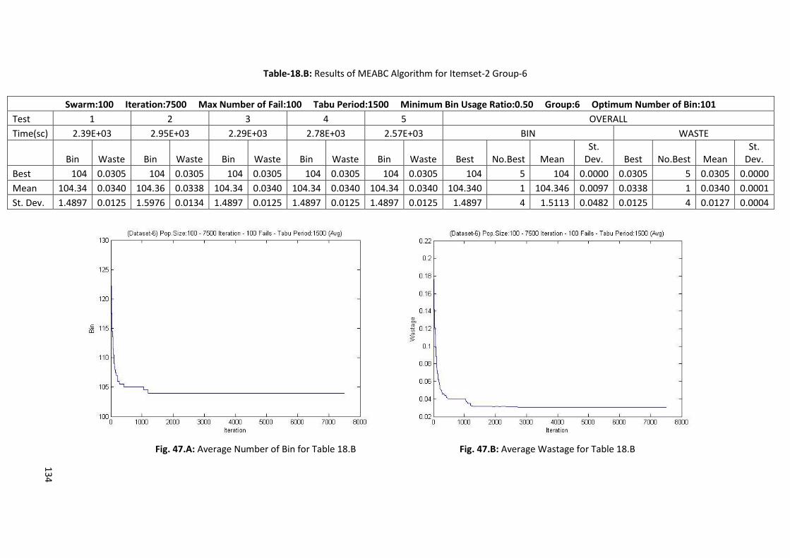
134

Table-18.B: Results of MEABC Algorithm for Itemset-2 Group-6

Swarm:100 Iteration:7500 Max Number of Fail:100 Tabu Period:1500 Minimum Bin Usage Ratio:0.50 Group:6 Optimum Number of Bin:101

Test 1 2 3 4 5 OVERALL

Time(sc) 2.39E+03 2.95E+03 2.29E+03 2.78E+03 2.57E+03 BIN WASTE

Bin Waste Bin Waste Bin Waste Bin Waste Bin Waste Best No.Best Mean St.

Dev. Best No.Best Mean St.

Dev.

Best 104 0.0305 104 0.0305 104 0.0305 104 0.0305 104 0.0305 104 5 104 0.0000 0.0305 5 0.0305 0.0000

Mean 104.34 0.0340 104.36 0.0338 104.34 0.0340 104.34 0.0340 104.34 0.0340 104.340 1 104.346 0.0097 0.0338 1 0.0340 0.0001

St. Dev. 1.4897 0.0125 1.5976 0.0134 1.4897 0.0125 1.4897 0.0125 1.4897 0.0125 1.4897 4 1.5113 0.0482 0.0125 4 0.0127 0.0004

Fig. 47.A: Average Number of Bin for Table 18.B Fig. 47.B: Average Wastage for Table 18.B

135

Table-18.C: Results of MEABC Algorithm for Itemset-2 Group-14

Swarm:100 Iteration:7500 Max Number of Fail:100 Tabu Period:1500 Minimum Bin Usage Ratio:0.50 Group:14 Optimum Number of Bin:103

Test 1 2 3 4 5 OVERALL

Time(sc) 2.33E+03 2.32E+03 2.32E+03 2.31E+03 2.57E+03 BIN WASTE

Bin Waste Bin Waste Bin Waste Bin Waste Bin Waste Best No.Best Mean St.

Dev. Best No.Best Mean St.

Dev.

Best 105 0.0290 105 0.0290 105 0.0290 105 0.0290 105 0.0290 105 5 105 0.0000 0.0290 5 0.0290 0.0000

Mean 105.99 0.0383 105.45 0.0341 105.68 0.0352 105.99 0.0383 105.68 0.0379 105.452 1 105.759 0.2323 0.0341 1 0.0368 0.0020

St. Dev. 1.4359 0.0117 1.5642 0.0128 1.4682 0.0124 1.4359 0.0117 1.4682 0.0124 1.4359 2 1.4744 0.0527 0.0117 2 0.0122 0.0005

Fig. 48.A: Average Number of Bin for Table 18.C Fig. 48.B: Average Wastage for Table 18.C

136

Table-18.D: Results of MEABC Algorithm for Itemset-2 Group-16

Swarm:100 Iteration:7500 Max Number of Fail:100 Tabu Period:1500 Minimum Bin Usage Ratio:0.50 Group:16 Optimum Number of Bin:105

Test 1 2 3 4 5 OVERALL

Time(sc) 2.12E+03 2.12E+03 2.13E+03 2.12E+03 2.35E+03 BIN WASTE

Bin Waste Bin Waste Bin Waste Bin Waste Bin Waste Best No.Best Mean St.

Dev. Best No.Best Mean St.

Dev.

Best 108 0.0295 108 0.0295 108 0.0295 108 0.0295 108 0.0295 108 5 108 0.0000 0.0295 5 0.0295 0.0000

Mean 108.31 0.0323 108.34 0.0326 108.34 0.0356 108.34 0.0326 108.34 0.0326 108.306 1 108.333 0.0154 0.0323 1 0.0331 0.0014

St. Dev. 1.6077 0.0131 1.7157 0.0138 1.7247 0.0138 1.7197 0.0138 1.7188 0.0138 1.6077 1.0000 1.6973 0.0502 0.0131 1.0000 0.0137 0.0003

Fig. 49.A: Average Number of Bin for Table 18.D Fig. 49.B: Average Wastage for Table 18.D

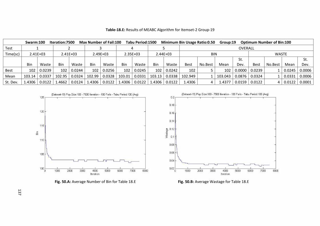
137

Table-18.E: Results of MEABC Algorithm for Itemset-2 Group-19

Swarm:100 Iteration:7500 Max Number of Fail:100 Tabu Period:1500 Minimum Bin Usage Ratio:0.50 Group:19 Optimum Number of Bin:100

Test 1 2 3 4 5 OVERALL

Time(sc) 2.41E+03 2.41E+03 2.49E+03 2.35E+03 2.44E+03 BIN WASTE

Bin Waste Bin Waste Bin Waste Bin Waste Bin Waste Best No.Best Mean St.

Dev. Best No.Best Mean St.

Dev.

Best 102 0.0239 102 0.0244 102 0.0256 102 0.0245 102 0.0242 102 5 102 0.0000 0.0239 1 0.0245 0.0006

Mean 103.14 0.0337 102.95 0.0324 102.99 0.0328 103.01 0.0331 103.13 0.0338 102.949 1 103.043 0.0876 0.0324 1 0.0331 0.0006

St. Dev. 1.4306 0.0122 1.4662 0.0124 1.4306 0.0122 1.4306 0.0122 1.4306 0.0122 1.4306 4 1.4377 0.0159 0.0122 4 0.0122 0.0001

Fig. 50.A: Average Number of Bin for Table 18.E Fig. 50.B: Average Wastage for Table 18.E

138

Fig. 51.A: MEABC Results for Number of Bin for Group-3 in Table-11 Fig. 51.B: MEABC Results for Wastage for Group-3 in Table-11

Fig. 52.A: MEABC Results for Number of Bin for Group-10 in Table-11 Fig. 52.B: MEABC Results for Wastage for Group-10 in Table-11

139

Fig. 53.A: MEABC Results for Number of Bin for Group-11 in Table-11 Fig. 53.B: MEABC Results for Wastage for Group-11 in Table-11

Fig. 54.A: MEABC Results for Number of Bin for Group-13 in Table-11 Fig. 54.B: MEABC Results for Wastage for Group-13 in Table-11

140

Fig. 55.A: MEABC Results for Number of Bin for Group-20 in Table-11 Fig. 55.B: MEABC Results for Wastage for Group-20 in Table-11

Fig. 56.A: MEABC Results for Number of Bin for Group-1 in Table-12 Fig. 56.B: MEABC Results for Wastage for Group-1 in Table-12

141

Fig. 57.A: MEABC Results for Number of Bin for Group-7 in Table-12 Fig. 57.B: MEABC Results for Wastage for Group-7 in Table-12

Fig. 58.A: MEABC Results for Number of Bin for Group-8 in Table-12 Fig. 58.B: MEABC Results for Wastage for Group-8 in Table-12

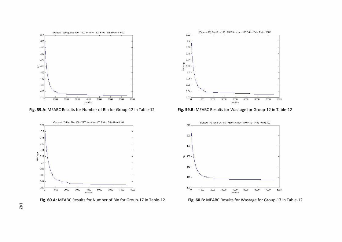
142

Fig. 59.A: MEABC Results for Number of Bin for Group-12 in Table-12 Fig. 59.B: MEABC Results for Wastage for Group-12 in Table-12

Fig. 60.A: MEABC Results for Number of Bin for Group-17 in Table-12 Fig. 60.B: MEABC Results for Wastage for Group-17 in Table-12

143

Table-19.A: Results of MEABC Algorithm for Itemset-5 Group-2

Swarm:100 Iteration:7500 Max Number of Fail:100 Tabu Period:1500 Minimum Bin Usage Ratio:0.50 Group:2 Optimum Number of Bin:20

Test 1 2 3 4 5 OVERALL

Time(sc) 457.2651 436.4584 456.7254 435.5143 436.4947 BIN WASTE

Bin Waste Bin Waste Bin Waste Bin Waste Bin Waste Best No.Best Mean St.

Dev. Best No.Best Mean St.

Dev.

Best 20 0.0213 21 0.0476 20 0.0232 21 0.0476 20 0.0222 20 3 20.4 0.5477 0.0213 1 0.0324 0.0139

Mean 20.994 0.0476 21.002 0.0478 20.986 0.0473 21.002 0.0477 20.970 0.0469 20.970 1 20.991 0.0132 0.0469 1 0.0475 0.0003

St. Dev. 0.1147 0.0039 0.0490 0.0025 0.1268 0.0034 0.0490 0.0022 0.1756 0.0048 0.0490 1 0.1030 0.0544 0.0022 1 0.0034 0.0010

Fig. 61.A: Average Number of Bin for Table 19.A Fig. 61.B: Average Wastage for Table 19.A

144

Table-19.B: Results of MEABC Algorithm for Itemset-5 Group-4

Swarm:100 Iteration:7500 Max Number of Fail:100 Tabu Period:1500 Minimum Bin Usage Ratio:0.50 Group:4 Optimum Number of Bin:20

Test 1 2 3 4 5 OVERALL

Time(sc) 480.8087 495.2828 494.6943 567.498 486.1935 BIN WASTE

Bin Waste Bin Waste Bin Waste Bin Waste Bin Waste Best No.Best Mean St.

Dev. Best No.Best Mean St.

Dev.

Best 21 0.0476 21 0.0476 21 0.0476 20 0.0195 21 0.0476 20 1 20.8 0.4472 0.0195 1 0.0420 0.0126

Mean 21.003 0.0479 21.003 0.0478 21.003 0.0478 20.982 0.0473 21.003 0.048 20.982 1 20.999 0.0092 0.0473 1 0.0478 0.0003

St. Dev. 0.0599 0.0030 0.0600 0.0028 0.0663 0.0031 0.1477 0.0047 0.0673 0.0035 0.0599 1 0.0802 0.0379 0.0028 1 0.0034 0.0007

Fig. 62.A: Average Number of Bin for Table 19.B Fig. 62.B: Average Wastage for Table 19.B

145

Table-19.C: Results of MEABC Algorithm for Itemset-5 Group-9

Swarm:100 Iteration:7500 Max Number of Fail:100 Tabu Period:1500 Minimum Bin Usage Ratio:0.50 Group:9 Optimum Number of Bin:20

Test 1 2 3 4 5 OVERALL

Time(sc) 462.9617 457.4456 470.7717 461.7659 438.9319 BIN WASTE

Bin Waste Bin Waste Bin Waste Bin Waste Bin Waste Best No.Best Mean St.

Dev. Best No.Best Mean St.

Dev.

Best 21 0.0476 21 0.0476 20 0.0231 21 0.0476 21 0.0476 20 1 20.8 0.4472 0.0231 1 0.0427 0.0110

Mean 21.002 0.0478 21.001 0.0477 20.985 0.0473 21.002 0.0477 21.002 0.0477 20.985 1 20.998 0.0073 0.0473 1 0.0477 0.0002

St. Dev. 0.0516 0.0027 0.0365 0.0020 0.1363 0.0039 0.0554 0.0027 0.0516 0.0024 0.0365 1 0.0663 0.0398 0.0020 1 0.0027 0.0007

Fig. 63.A: Average Number of Bin for Table 19.C Fig. 63.B: Average Wastage for Table 19.C

146

Table-19.D: Results of MEABC Algorithm for Itemset-5 Group-15

Swarm:100 Iteration:7500 Max Number of Fail:100 Tabu Period:1500 Minimum Bin Usage Ratio:0.50 Group:15 Optimum Number of Bin:20

Test 1 2 3 4 5 OVERALL

Time(sc) 478.2567 531.6818 441.1302 452.9791 446.3824 BIN WASTE

Bin Waste Bin Waste Bin Waste Bin Waste Bin Waste Best No.Best Mean St.

Dev. Best No.Best Mean St.

Dev.

Best 20 0.0230 21 0.0476 21 0.0476 20 0.0237 21 0.0476 20 2 20.6 0.5477 0.0230 1 0.0379 0.0133

Mean 20.987 0.0474 21.002 0.0478 21.002 0.0478 20.986 0.0474 21.001 0.0478 20.986 1.0000 20.996 0.0084 0.0474 1.0000 0.0476 0.0002

St. Dev. 0.1310 0.0040 0.0600 0.0028 0.0622 0.0029 0.1393 0.0041 0.0447 0.0024 0.0447 1 0.0874 0.0442 0.0024 1 0.0033 0.0008

Fig. 64.A: Average Number of Bin for Table 19.D Fig. 64.B: Average Wastage for Table 19.D

147

Table-19.E: Results of MEABC Algorithm for Itemset-5 Group-18

Swarm:100 Iteration:7500 Max Number of Fail:100 Tabu Period:1500 Minimum Bin Usage Ratio:0.50 Group:18 Optimum Number of Bin:20

Test 1 2 3 4 5 OVERALL

Time(sc) 472.2183 442.9414 442.5902 487.3755 458.3236 BIN WASTE

Bin Waste Bin Waste Bin Waste Bin Waste Bin Waste Best No.Best Mean St.

Dev. Best No.Best Mean St.

Dev.

Best 21 0.0476 20 0.0239 21 0.0476 21 0.0476 21 0.0476 20 1 20.8 0.4472 0.0239 1 0.0429 0.0106

Mean 21.002 0.0478 20.983 0.0473 21.003 0.0478 21.003 0.0478 21.002 0.0478 20.983 1 20.999 0.0085 0.0473 1 0.0477 0.0002

St. Dev. 0.0632 0.0029 0.1442 0.0041 0.0682 0.0032 0.0621 0.0031 0.0516 0.0025 0.0516 1 0.0779 0.0376 0.0025 1 0.0032 0.0006

Fig. 65.A: Average Number of Bin for Table 19.E Fig. 65.B: Average Wastage for Table 19.E

148

Table-20.A: Results of MEABC Algorithm for Itemset-6 Group-2

Swarm:100 Iteration:7500 Max Number of Fail:100 Tabu Period:1500 Minimum Bin Usage Ratio:0.50 Group:2 Optimum Number of Bin:40

Test 1 2 3 4 5 OVERALL

Time(sc) 1.08E+03 1.06E+03 1.05E+03 1.11E+03 1.05E+03 BIN WASTE

Bin Waste Bin Waste Bin Waste Bin Waste Bin Waste Best No.Best Mean St.

Dev. Best No.Best Mean St.

Dev.

Best 41 0.0347 41 0.0335 41 0.0353 42 0.0476 41 0.0345 41 4 41.2 0.4472 0.0335 1 0.0371 0.0059

Mean 42.211 0.0535 42.003 0.0480 42.005 0.0478 42.015 0.0481 42.004 0.0479 42.003 1 42.047 0.0913 0.0478 1 0.0491 0.0025

St. Dev. 0.5227 0.0107 0.2414 0.0050 0.2016 0.0043 0.2124 0.0047 0.2318 0.0048 0.2016 1 0.2820 0.1355 0.0043 1 0.0059 0.0027

Fig. 66.A: Average Number of Bin for Table 20.A Fig. 66.B: Average Wastage for Table 20.A

149

Table-20.B: Results of MEABC Algorithm for Itemset-6 Group-3

Swarm:100 Iteration:7500 Max Number of Fail:100 Tabu Period:1500 Minimum Bin Usage Ratio:0.50 Group:3 Optimum Number of Bin:40

Test 1 2 3 4 5 OVERALL

Time(sc) 1.06E+03 1.06E+03 1.06E+03 1.06E+03 1.05E+03 BIN WASTE

Bin Waste Bin Waste Bin Waste Bin Waste Bin Waste Best No.Best Mean St.

Dev. Best No.Best Mean St.

Dev.

Best 42 0.0476 42 0.0536 42 0.0476 42 0.0476 42 0.0537 42 5 42 0.0000 0.0476 1 0.0500 0.0033

Mean 42.013 0.0481 42.813 0.0671 42.019 0.0483 42.014 0.0481 42.79 0.0668 42.013 1 42.33 0.4306 0.0481 1 0.0557 0.0103

St. Dev. 0.1872 0.0042 0.4220 0.0066 0.2143 0.0048 0.1982 0.0044 0.4416 0.0068 0.1872 1 0.2926 0.1276 0.0042 1 0.0054 0.0012

Fig. 67.A: Average Number of Bin for Table 20.B Fig. 67.B: Average Wastage for Table 20.B

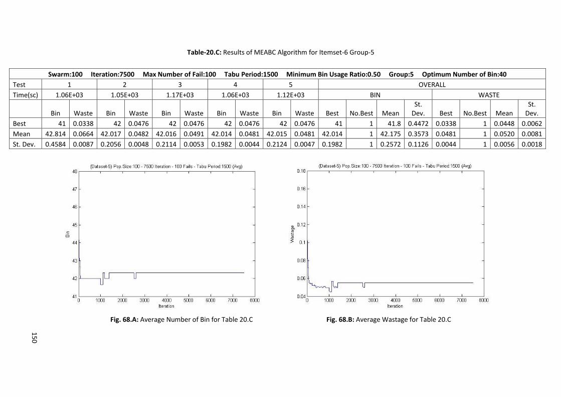
150

Table-20.C: Results of MEABC Algorithm for Itemset-6 Group-5

Swarm:100 Iteration:7500 Max Number of Fail:100 Tabu Period:1500 Minimum Bin Usage Ratio:0.50 Group:5 Optimum Number of Bin:40

Test 1 2 3 4 5 OVERALL

Time(sc) 1.06E+03 1.05E+03 1.17E+03 1.06E+03 1.12E+03 BIN WASTE

Bin Waste Bin Waste Bin Waste Bin Waste Bin Waste Best No.Best Mean St.

Dev. Best No.Best Mean St.

Dev.

Best 41 0.0338 42 0.0476 42 0.0476 42 0.0476 42 0.0476 41 1 41.8 0.4472 0.0338 1 0.0448 0.0062

Mean 42.814 0.0664 42.017 0.0482 42.016 0.0491 42.014 0.0481 42.015 0.0481 42.014 1 42.175 0.3573 0.0481 1 0.0520 0.0081

St. Dev. 0.4584 0.0087 0.2056 0.0048 0.2114 0.0053 0.1982 0.0044 0.2124 0.0047 0.1982 1 0.2572 0.1126 0.0044 1 0.0056 0.0018

Fig. 68.A: Average Number of Bin for Table 20.C Fig. 68.B: Average Wastage for Table 20.C

151

Table-20.D: Results of MEABC Algorithm for Itemset-6 Group-14

Swarm:100 Iteration:7500 Max Number of Fail:100 Tabu Period:1500 Minimum Bin Usage Ratio:0.50 Group:14 Optimum Number of Bin:40

Test 1 2 3 4 5 OVERALL

Time(sc) 1.05E+03 1.11E+03 1.05E+03 1.17E+03 1.06E+03 BIN WASTE

Bin Waste Bin Waste Bin Waste Bin Waste Bin Waste Best No.Best Mean St.

Dev. Best No.Best Mean St.

Dev.

Best 41 0.0345 42 0.0476 41 0.0342 42 0.0537 41 0.0347 41 3 41.4 0.5477 0.0342 1 0.0409 0.0091

Mean 42.004 0.0479 42.014 0.0481 41.991 0.0477 42.79 0.0668 42.211 0.0535 41.991 1 42.202 0.3408 0.0477 1 0.0528 0.0082

St. Dev. 0.2318 0.0048 0.1982 0.0044 0.2632 0.0051 0.4416 0.0068 0.5227 0.0107 0.1982 1 0.3315 0.1423 0.0044 1 0.0064 0.0026

Fig. 69.A: Average Number of Bin for Table 20.D Fig. 69.B: Average Wastage for Table 20.D

152

Table-20.E: Results of MEABC Algorithm for Itemset-6 Group-18

Swarm:100 Iteration:7500 Max Number of Fail:100 Tabu Period:1500 Minimum Bin Usage Ratio:0.50 Group:18 Optimum Number of Bin:40

Test 1 2 3 4 5 OVERALL

Time(sc) 1.12E+03 1.10E+03 1.14E+03 1.06E+03 1.08E+03 BIN WASTE

Bin Waste Bin Waste Bin Waste Bin Waste Bin Waste Best No.Best Mean St.

Dev. Best No.Best Mean St.

Dev.

Best 42 0.0476 42 0.0537 42 0.0476 42 0.0536 42 0.0536 42 5 42 0.0000 0.0476 1 0.0512 0.0033

Mean 42.015 0.0481 42.79 0.0668 42.016 0.0484 42.813 0.0671 42.813 0.0671 42.015 1 42.489 0.4327 0.0481 1 0.0595 0.0103

St. Dev. 0.2124 0.0047 0.4416 0.0068 0.2245 0.0052 0.4220 0.0066 0.4220 0.0066 0.2124 1 0.3445 0.1154 0.0047 1 0.0060 0.0010

Fig. 70.A: Average Number of Bin for Table 20.E Fig. 70.B: Average Wastage for Table 20.E

153

Table-21.A: Results of MEABC Algorithm for Itemset-7 Group-1

Swarm:100 Iteration:7500 Max Number of Fail:100 Tabu Period:1500 Minimum Bin Usage Ratio:0.50 Group:1 Optimum Number of Bin:83

Test 1 2 3 4 5 OVERALL

Time(sc) 1.99E+03 2.00E+03 1.85E+03 1.96E+03 1.95E+03 BIN WASTE

Bin Waste Bin Waste Bin Waste Bin Waste Bin Waste Best No.Best Mean St.

Dev. Best No.Best Mean St.

Dev.

Best 88 0.0568 87 0.0510 88 0.0574 88 0.0578 87 0.0584 87 2 87.6 0.5477 0.0510 1 0.0563 0.0030

Mean 88.056 0.0576 88.043 0.0574 88.075 0.0587 88.063 0.0579 88.044 0.0582 88.043 1 88.056 0.0136 0.0574 1 0.0580 0.0005

St. Dev. 0.5613 0.0057 0.6108 0.0061 0.5572 0.0057 0.5698 0.0058 0.6188 0.0060 0.5572 1 0.5836 0.0290 0.0057 1 0.0059 0.0002

Fig. 71.A: Average Number of Bin for Table 21.A Fig. 71.B: Average Wastage for Table 21.A

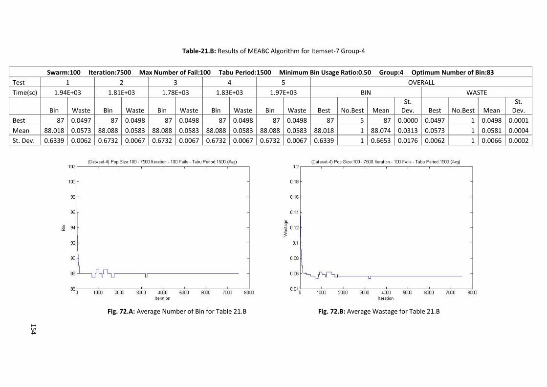
154

Table-21.B: Results of MEABC Algorithm for Itemset-7 Group-4

Swarm:100 Iteration:7500 Max Number of Fail:100 Tabu Period:1500 Minimum Bin Usage Ratio:0.50 Group:4 Optimum Number of Bin:83

Test 1 2 3 4 5 OVERALL

Time(sc) 1.94E+03 1.81E+03 1.78E+03 1.83E+03 1.97E+03 BIN WASTE

Bin Waste Bin Waste Bin Waste Bin Waste Bin Waste Best No.Best Mean St.

Dev. Best No.Best Mean St.

Dev.

Best 87 0.0497 87 0.0498 87 0.0498 87 0.0498 87 0.0498 87 5 87 0.0000 0.0497 1 0.0498 0.0001

Mean 88.018 0.0573 88.088 0.0583 88.088 0.0583 88.088 0.0583 88.088 0.0583 88.018 1 88.074 0.0313 0.0573 1 0.0581 0.0004

St. Dev. 0.6339 0.0062 0.6732 0.0067 0.6732 0.0067 0.6732 0.0067 0.6732 0.0067 0.6339 1 0.6653 0.0176 0.0062 1 0.0066 0.0002

Fig. 72.A: Average Number of Bin for Table 21.B Fig. 72.B: Average Wastage for Table 21.B

155

Table-21.C: Results of MEABC Algorithm for Itemset-7 Group-9

Swarm:100 Iteration:7500 Max Number of Fail:100 Tabu Period:1500 Minimum Bin Usage Ratio:0.50 Group:9 Optimum Number of Bin:83

Test 1 2 3 4 5 OVERALL

Time(sc) 1.99E+03 1.89E+03 1.95E+03 1.83E+03 1.95E+03 BIN WASTE

Bin Waste Bin Waste Bin Waste Bin Waste Bin Waste Best No.Best Mean St.

Dev. Best No.Best Mean St.

Dev.

Best 87 0.0493 87 0.0495 87 0.0495 87 0.0495 87 0.0495 87 5 87 0.0000 0.0493 1 0.0495 0.0001

Mean 88.033 0.0573 88.023 0.0573 88.023 0.0573 88.023 0.0573 88.023 0.0573 88.023 4 88.025 0.0047 0.0573 1 0.0573 0.0000

St. Dev. 0.6448 0.0063 0.6800 0.0066 0.6800 0.0066 0.6800 0.0066 0.6800 0.0066 0.6448 1 0.6729 0.0157 0.0063 1 0.0065 0.0001

Fig. 73.A: Average Number of Bin for Table 21.C Fig. 73.B: Average Wastage for Table 21.C

156

Table-21.D: Results of MEABC Algorithm for Itemset-7 Group-11

Swarm:100 Iteration:7500 Max Number of Fail:100 Tabu Period:1500 Minimum Bin Usage Ratio:0.50 Group:11 Optimum Number of Bin:83

Test 1 2 3 4 5 OVERALL

Time(sc) 1.88E+03 1.73E+03 1.97E+03 1.81E+03 1.94E+03 BIN WASTE

Bin Waste Bin Waste Bin Waste Bin Waste Bin Waste Best No.Best Mean St.

Dev. Best No.Best Mean St.

Dev.

Best 87 0.0495 87 0.0460 87 0.0495 87 0.0495 87 0.0495 87 5 87 0.0000 0.0460 1 0.0488 0.0016

Mean 88.048 0.0575 87.139 0.0478 88.048 0.0575 88.048 0.0575 88.048 0.0575 87.139 1 87.866 0.4068 0.0478 1 0.0555 0.0043

St. Dev. 0.6266 0.0063 0.7371 0.0079 0.6266 0.0063 0.6266 0.0063 0.6266 0.0063 0.6266 4 0.6487 0.0494 0.0063 4 0.0066 0.0007

Fig. 74.A: Average Number of Bin for Table 21.D Fig. 74.B: Average Wastage for Table 21.D

157

Table-21.E: Results of MEABC Algorithm for Itemset-7 Group-15

Swarm:100 Iteration:7500 Max Number of Fail:100 Tabu Period:1500 Minimum Bin Usage Ratio:0.50 Group:15 Optimum Number of Bin:83

Test 1 2 3 4 5 OVERALL

Time(sc) 1.83E+03 1.95E+03 1.96E+03 2.00E+03 1.73E+03 BIN WASTE

Bin Waste Bin Waste Bin Waste Bin Waste Bin Waste Best No.Best Mean St.

Dev. Best No.Best Mean St.

Dev.

Best 87 0.0498 87 0.0490 87 0.0498 87 0.0493 87 0.0510 87 5 87 0.0000 0.0490 1 0.0498 0.0008

Mean 87.977 0.0569 87.995 0.0570 87.977 0.0569 88.033 0.0573 88.043 0.0574 87.977 2 88.005 0.0312 0.0569 2 0.0571 0.0002

St. Dev. 0.6660 0.0063 0.6699 0.0064 0.6660 0.0063 0.6448 0.0063 0.6108 0.0061 0.6108 1 0.6515 0.0248 0.0061 1 0.0063 0.0001

Fig. 75.A: Average Number of Bin for Table 21.E Fig. 75.B: Average Wastage for Table 21.E

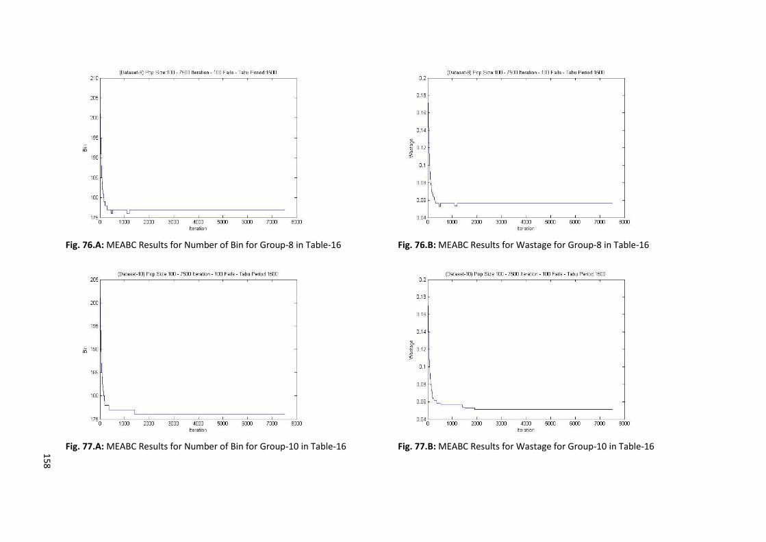
158

Fig. 76.A: MEABC Results for Number of Bin for Group-8 in Table-16 Fig. 76.B: MEABC Results for Wastage for Group-8 in Table-16

Fig. 77.A: MEABC Results for Number of Bin for Group-10 in Table-16 Fig. 77.B: MEABC Results for Wastage for Group-10 in Table-16

159

Fig. 78.A: MEABC Results for Number of Bin for Group-13 in Table-16 Fig. 78.B: MEABC Results for Wastage for Group-13 in Table-16

Fig. 79.A: MEABC Results for Number of Bin for Group-16 in Table-16 Fig. 79.B: MEABC Results for Wastage for Group-16 in Table-16

160

Fig. 80.A: MEABC Results for Number of Bin for Group-19 in Table-16 Fig. 80.B: MEABC Results for Wastage for Group-19 in Table-16