determinants of mobile apps success: evidence from app ... · many mobile application markets such...
TRANSCRIPT
1
Determinants of Mobile Apps Success:
Evidence from App Store Market
GUNWOONG LEE AND T. S. RAGHU
Department of Information Systems, W.P. Carey School of Business
Arizona State University
Tempe, AZ 85287-4606
[email protected]; [email protected]
GUNWOONG LEE is a Ph.D. candidate of Information Systems at the W. P. Carey School of
Business, Arizona State University. His research interests include digital content management in
mobile platforms, information and communication technology for development, and technology-
driven healthcare innovations. His research has appeared in major conferences and journals
including Decision Support Systems, International Conference on Information Systems, and
America Conference on Information Systems. He has consulting experience with Korea
Association of Game Industry, Korea Stock Exchange, and other companies and government
agencies.
RAGHU T. S. is a Professor of Information Systems in the W. P. Carey School of Business at
Arizona State University. His current research focuses on Health Information Technology,
Services Design and Consumer Informatics. He has published a number of scholarly articles on
Business Process and Services design, Electronic Medical Records (EMR) adoption and impacts,
Personal Health Records (PHR) adoption, and technology based decision support. He has served
on or currently serves on the Editorial Boards of a number of peer-reviewed journals including
Information Systems Research, Decision Support Systems, Journal of the Association for
Information Systems, and Journal of Electronic Commerce Research. He is an advisory editor of
the Elsevier series on “Handbooks in Information Systems.” Professor Raghu recently served as
the Program Co-Chair for Workshop on E-Business, 2009 and as Program Co-Chair for
INFORMS Conference on Information Systems and Technology (CIST), 2012.
2
Abstract
Mobile applications markets with App stores have introduced a new approach to define and sell
software applications with access to a large body of heterogeneous consumer population. This
research examines key seller- and App-level characteristics that impact success in an App store
market. We tracked individual Apps and their presence in the top grossing 300 charts in Apple
App Store and examined how factors at different levels affect the Apps’ survival in the top 300
charts. We used a generalized hierarchical modeling approach to measure sales performance,
and confirmed the results with the use of a hazard model and a count regression model. We find
that broadening App offerings across multiple categories is a key determinant that contributes to
a higher probability of survival in the top charts. App-level attributes such as free App offers,
high initial ranks, investment in less popular (less competitive) categories, continuous quality
updates, and high volume and high user review scores have positive impacts on Apps’
sustainability. In general, each diversification decision across a category results in
approximately a 15% increase in the presence of an App in the top charts. Survival rates for free
Apps are up to two times more than that for paid Apps. Quality (feature) updates to Apps can
contribute up to a three-fold improvement in survival rate as well. A key implication of the
results is that sellers must utilize the natural segmentation in consumer tastes offered by the
different categories to improve sales performance.
Keywords: App store market, mobile software sustainability, product portfolio management,
survival analysis.
3
Determinants of Mobile Apps Success:
Evidence from App Store Market
Introduction
Variety's the very spice of life, That gives it all its flavor
- William Cowper, 1785
Mobile applications are one of the fastest growing segments of downloadable software
applications markets. Many mobile application markets such as Amazon Appstore, Blackberry
App World, Google Play Store, and Apple App Store have emerged and grown rapidly in a short
amount of time. Since Apple App Store (henceforth, AppStore) launched with only 500 Apps
and a dozen developers in July 2008, the market has increased to over 845,900 Apps and
226,500 unique sellers in April 20131. This rapidly growing market has in turn led to over 500
million AppStore users downloading around 40 billion Apps in 155 countries and the platform
had paid out over 7 billion dollars to App developers in 20122.
Mobile App store markets exhibit key characteristics of “long tail market” [3] such as a large
selection of digital products and relatively low user search costs. However, App store market
structure has some key differentiating characteristics that set it apart from a number of previously
examined long-tail market contexts such as books [13], music [29], and movies [26, 36]. First,
sellers in mobile App markets have a single channel for selling their product (especially in case
of Apple’s App market) and terms of access to the market are uniformly determined for all
1 Apple’s App Store Report (April, 15
th, 2013), 148Apps, available at http://148apps.biz/app-store-metrics/
2 App Store Tops 40 Billion Downloads with Almost Half in 2012 (January 17
th , 2013), Apple, available at
http://www.apple.com/pr/library/2013/01/07App-Store-Tops-40-Billion-Downloads-with-Almost-Half-in-2012.html
4
sellers. Second, unlike creators of music and DVDs, App developers/sellers have the opportunity
to change not only price, but also the features and characteristics of the App based on user
feedback and reviews. Third, sellers in mobile App markets compete more directly with other
developers, irrespective of whether Apps are intended for hedonic consumption (such as
crossword puzzles) or utilitarian purposes (e.g., teleprompters). Comparing competing Apps
within a category is easier than, say, comparing music offerings within a genre. Fourth, while in
many long-tail markets versioning is restricted to release times or superficial features (such as
hard-cover vs. paperback), mobile Apps offer a greater range of flexibility to sellers in
versioning strategies (e.g., feature based or price based differentiation, in-app purchases,
subscription length, etc.). Finally, sellers can reuse features and codebase from one App to
another, thereby quickly building a portfolio of Apps across various (and often unrelated) App
categories. The portfolio perspective, in fact, is the most distinguishing facet of mobile App
markets that we intend to explore in this research.
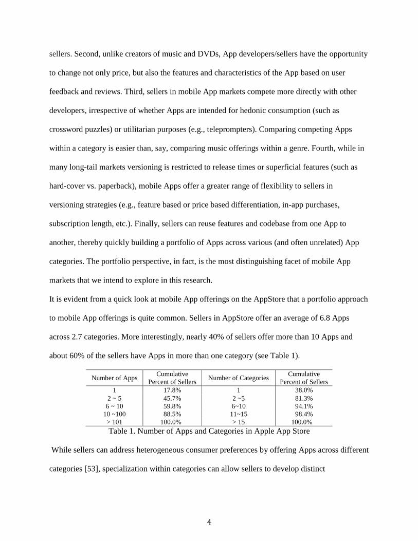
It is evident from a quick look at mobile App offerings on the AppStore that a portfolio approach
to mobile App offerings is quite common. Sellers in AppStore offer an average of 6.8 Apps
across 2.7 categories. More interestingly, nearly 40% of sellers offer more than 10 Apps and
about 60% of the sellers have Apps in more than one category (see Table 1).
Number of Apps Cumulative
Percent of Sellers Number of Categories
Cumulative
Percent of Sellers
1 17.8% 1 38.0%
2 ~ 5 45.7% 2 ~5 81.3%
6 ~ 10 59.8% 6~10 94.1%
10 ~100 88.5% 11~15 98.4%
> 101 100.0% > 15 100.0%
Table 1. Number of Apps and Categories in Apple App Store
While sellers can address heterogeneous consumer preferences by offering Apps across different
categories [53], specialization within categories can allow sellers to develop distinct

5
competencies and benefit from scope economies through reduced product development costs [9].
Using key tenets of product portfolio management theory and theory of economies of scope, this
study empirically investigates how sellers’ App portfolio strategies are associated with sales
performance over time. Utilizing a longitudinal panel data of sales performance over 39 weeks,
we model App survival in the weekly charts within App categories. We consider the impact of
both seller-level and App-level properties on an App’s survival in the top charts. Our main
research objective is to understand how sellers’ App portfolio affects sales sustainability in the
AppStore. We also intend to develop insights into how App specific decisions (such as free
offerings, price changes and updates) affect sales performance and sustainability of individual
Apps.
The key contributions of this research to the extant literature are as follows. First, we show that
specific portfolio properties affect sales performance sustainability in high velocity software
markets such as the Apple’s App Store. Using the rich data context of the App store market, we
overcome key methodological barriers to understanding portfolio impacts on sustained sales
performance. By utilizing three different types of models (a generalized hierarchical linear model,
a hazard model, and a count regression model), we provide empirical evidence to show how
sellers’ App portfolio management influences success in App markets. In general, we find that
each diversification decision across a category results in approximately a 15 % increase in
survival probability. Moreover, we find that free offering, higher debut rank, investment in less
popular categories, continuous feature updates, and higher user review scores on Apps have
positive impacts on Apps’ sustainability.
6
Theoretical Foundation
Product Portfolio Management
Day [25] defines product portfolio as “a decision on the use of managerial resources for
maximum long-run gains.” Extant marketing literature identifies two different product portfolio
management strategies: product proliferation and product concentration. By offering highly
divergent product lines, firms can satisfy consumers’ desire for variety seeking [4, 49] and meet
customer need in a manner superior to competitor’s product offerings [53]. However, in spite of
these merits of product diversification, some firms successfully pursue the opposite strategy of
concentrating on specific product lines. The narrower product line helps the firms to lower unit
production costs when scale economies are present by lowering inventory costs, and reducing
complexity in assembly. Hence, the success of product proliferation depends not only on the
firm’s market, but also on firm specific properties.
However, past research has found no evidence of a positive relationship between product
concentration and sales performance [21]. Many studies applying financial portfolio theory to
product portfolio management [17, 28] show that correlations across similar product categories
lead to a higher risk profile for the firm. Therefore, diversification of Apps over selling
categories has the potential to improve product portfolio’s risk-return profile.
There is still lack of research in understanding the association between information goods
portfolio management and sales performance. Extant research on long tail markets of
information goods such as DVDs and books have not considered product portfolio effects, but
only long tail properties and intermediation/disintermediation effects [13, 46]. Although
Brynjolffson [14] suggested a research agenda that studies shifts in product variety and
concentration patterns driven by information technology, their research focus is still limited to an
7
issue of shaping a long tail (broadening niche products for product variety) or Superstar effect
(concentrating on a few popular products for product concentration). However, as Brynjolffson
[14] suggest, technological (changes in search, personalization, and online community
technologies) drivers and non-technological drivers (price premium and social interactions with
other consumers) have shifted the consumption and production patterns of niche and popular
products. In App store markets, technological drivers are playing an especially important role in
increasing sellers’ incentives to create various Apps with a lower barrier to entry and a large
network of users, while also increasing users’ incentives to purchase Apps that satisfy their tastes
with lower search costs and a large selection of Apps.
A key driver of portfolio decisions in App store markets will be the ability to create scope
economies by developing and leveraging product development capabilities across a number of
different categories of mobile App offerings. We argue that the lower barriers to entering
different category segments enables sellers to expand their offerings beyond what has been
considered in product portfolio literature. Additionally, the ability to alter App offerings based
on specific information gleaned from sales, usage patterns, and user feedback enables sellers to
update their product offerings almost on a constant basis, thus setting up a high velocity market
environment. We expand on the notion of scope economy in the following paragraphs.
Scope Economies
The theory of scope economies provides a rationale for associating broadening product selections
with sales performance. Economies of scope refer to the cost and revenue benefits through the
production of a wider variety of products across related settings rather than specializing in the
production of a single product [39, 48]. A firm’s ability to leverage investment experience and
8
knowledge from one setting to another can confer significant performance benefits. Bailey and
Friedlaender [8] argue that firm-level scope economies are crucial for multi-product industries
and present that, in a competitive market, multi-product firms better survive as compared to
single-product competitors since the economies of scope bring about a significant cost advantage
(e.g., transaction costs) to those firms. In this context, Cottrell and Nault [22] utilized the theory
of scope economies in production and consumption to examine the association between product
variety and scope economies in the microcomputer software industry in the 1980s by using firm-
and product-level information on bundling of functionalities over application categories and
computing platforms. The main results indicate that there are scope economies in the
consumption of microcomputer software, and so firms with software that includes more
application categories (e.g., database, graphics, and word processor) have better sales
performance and product survival since a customer may prefer to purchase a variety of products
from the same vendor. There are several distinctive characteristics of the App market that
warrant examination of scope economies in App markets. For example, at the outset, scope
economies in production appear to be much stronger in App markets because of the predominant
focus on hedonic consumption as opposed to utilitarian consumption [5]. On the other hand,
hedonic consumption can also contribute to a diminished importance of scope economies in
consumption since interoperability between Apps may not yet be of great importance to
consumers [20, 35]. App markets are also distinct from software markets of the 80’s in that there
is a single distribution channel today for Apps and channel access is not constrained for any
single type of sellers. Examination of App portfolio related issues is still nascent in IS literature.
Most recently, Lee and Raghu [40] used a cross-sectional analysis of portfolio decisions in the
App market to demonstrate that App portfolio diversification over multiple categories is
9
positively correlated with success in App sales. In this research, we utilize data at multiple levels
(seller and App properties) to examine longitudinal impacts on sales performance.
In summary, consistent with main tenets in theory of product portfolio management and theory
of scope economies, we predict that a large selection of mobile Apps (i.e., the number of
products) and diversification across selling categories (i.e., product diversity) increase the
success of App sales. In the following section, we outline our research approach by describing
the empirical models and data collection.
Empirical Approach and Data Descriptions
Survival Analysis
The main empirical question in this study is the sustainability of sales over time. To establish the
association between a seller’s App portfolio characteristic and Apps’ sustainability in the top
charts, we utilize multiple approaches. Our definition of success is restricted to
appearance/reappearance of Apps in the top-charts over time. Since Apps can frequently appear
and disappear on top charts, both survival duration (between an appearance and disappearance)
and the total length of time spent on the top charts are relevant measures of success. Therefore,
we use survival analysis techniques to measure sales performance [22, 56]. We observe survival
(or exit) for all products and all sellers, and survival of the App in the top charts is a necessary
condition for success. Finally, the exit of an App for extended durations from the top charts can
indicate poor performance [54].
In our empirical model, the success of App sales is influenced by a seller’s decisions at two
levels. At the App-level, seller decisions frame certain App-specific properties before launch
such as category, price, and certain properties after launch such as quality and price updates. A
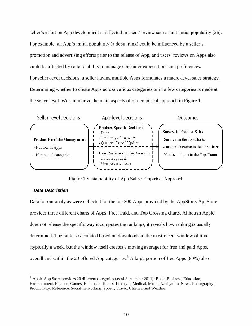
10
seller’s effort on App development is reflected in users’ review scores and initial popularity [26].
For example, an App’s initial popularity (a debut rank) could be influenced by a seller’s
promotion and advertising efforts prior to the release of App, and users’ reviews on Apps also
could be affected by sellers’ ability to manage consumer expectations and preferences.
For seller-level decisions, a seller having multiple Apps formulates a macro-level sales strategy.
Determining whether to create Apps across various categories or in a few categories is made at
the seller-level. We summarize the main aspects of our empirical approach in Figure 1.
Figure 1.Sustainability of App Sales: Empirical Approach
Data Description
Data for our analysis were collected for the top 300 Apps provided by the AppStore. AppStore
provides three different charts of Apps: Free, Paid, and Top Grossing charts. Although Apple
does not release the specific way it computes the rankings, it reveals how ranking is usually
determined. The rank is calculated based on downloads in the most recent window of time
(typically a week, but the window itself creates a moving average) for free and paid Apps,
overall and within the 20 offered App categories.3 A large portion of free Apps (80%) also
3 Apple App Store provides 20 different categories (as of September 2011): Book, Business, Education,
Entertainment, Finance, Games, Healthcare-fitness, Lifestyle, Medical, Music, Navigation, News, Photography,
Productivity, Reference, Social-networking, Sports, Travel, Utilities, and Weather.
11
includes in-app-purchase options. In order to complement the limitations of free and paid charts,
we used the top grossing charts, thus combining free and paid Apps in a single chart.
We collected the top-charts data for each week, on a specific day of the week, from December
2010 to September 2011. During this period of 39 weeks, a total of 17,697 Apps offered by
8,627 unique sellers appeared on the chart (a total of 530,503 observations). To observe an App’s
and a seller’ discrete survival at a specific study week and survival duration in the top 300, 200
and 100 charts, we tracked an individual App’s (seller’s) elapsed time to list in the top 300 by
using data from Apple’s iTunes. Every App in the dataset has its release time and the first time to
hit the top 300. The Apps released before the starting date of data collection were censored since
we are not able to observe key App properties in the past. Therefore, Apps that made the top 300
chart before the study period were dropped from the dataset. However, an App released after our
data collection date (Week 1) has both (1) valid released date and (2) the first date to hit the top
chart. Time (1) and time (2) could be the same when an App was ranked in the top 300 at its
debut week.
The iTunes store provides individual App’s rank, seller (or publisher), title, price, category,
released date, updated date, description, user review score, and number of user reviews. From
given information on Apps, we tracked the survival of individual App at each study week,
calculated elapsed time of individual App to exist in the top charts, and obtained data on each
seller’s specific properties such as total number of Apps and number of categories in the top 300,
200, and 100 charts. Finally, we validated our data by comparing the actual figures (e.g., a
portion of free Apps, a seller’s number of Apps/categories, and a portion of (un)popular
categories in AppStore) produced by popular mobile application tracking websites: App148.biz
(information on the number of Apps under different categories and prices) and AppStoreHQ.com
12
(seller’s information), and we confirmed our descriptive statistics were very close to those
figures.
Data for Survival Analysis
We created two different sets of data for analyzing App success (an App’s survival) at each
discrete point in time and survival duration in the top charts). To record the survival of an App as
a discrete time event, we tracked all Apps that Appeared in the top 300 charts during the study
period, and coded an App that appeared in the chart as a survival (“1”), or otherwise as an exit
(“0”) if the App dropped from the charts. The discrete event approach does not pose censoring
issues.
Survival duration relied on a continuous time scale and therefore had to censor some
observations. When survival data is analyzed on a continuous time scale (e.g., hazard models),
all observations in the sample may not have terminated or the exact initial times of all events
may not be known [45]. This was an issue in our data as well. For the 300 top grossing charts,
we censored 66.3% from the observed Apps as follows: Apps that already appeared before the
study (left-censoring), were still alive at the end of study (right-censoring), and exited and
reappeared over the study period (interval-censoring) were cut off. Thus, the final dataset for
continuous survival time analysis consisted of 7,579 Apps in the top 300 charts provided by
3,882 sellers. The set of variables extracted from our dataset is shown in Table 2.
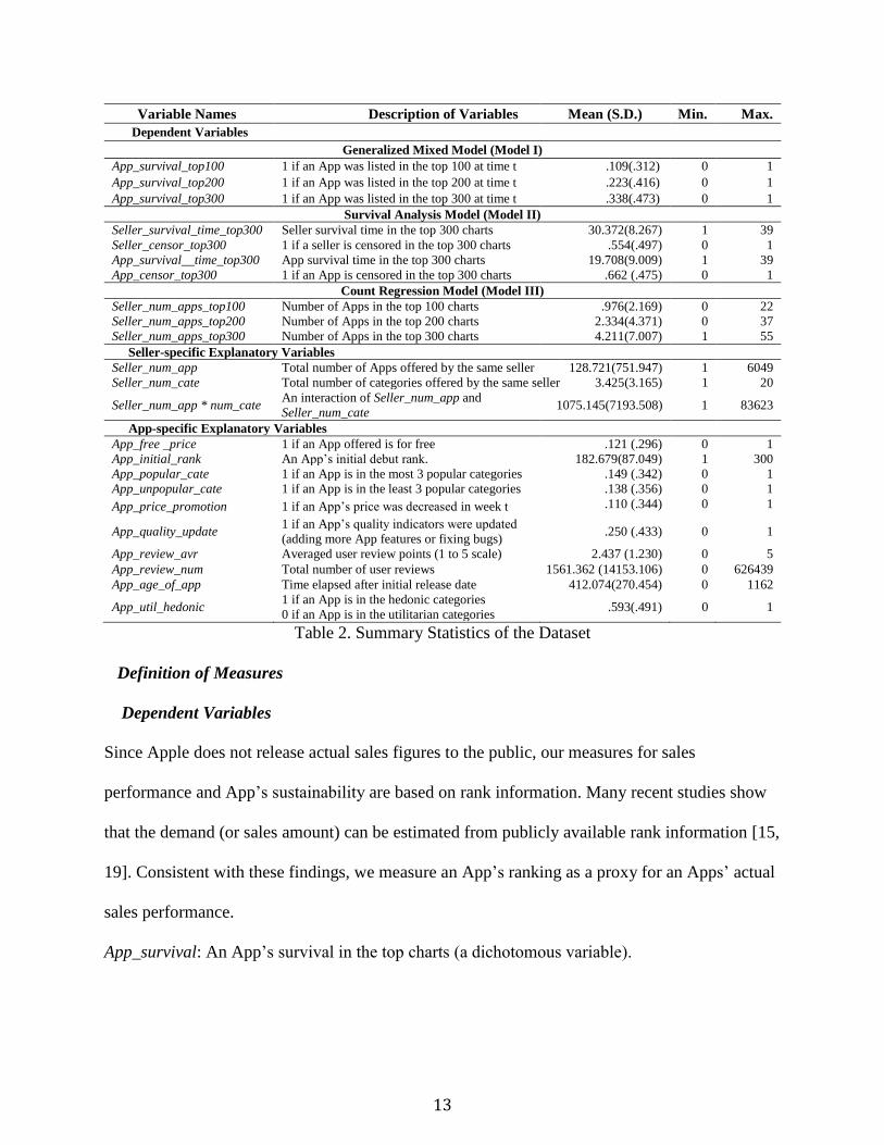
13
Variable Names Description of Variables Mean (S.D.) Min. Max.
Dependent Variables
Generalized Mixed Model (Model I)
App_survival_top100 1 if an App was listed in the top 100 at time t .109(.312) 0 1
App_survival_top200 1 if an App was listed in the top 200 at time t .223(.416) 0 1
App_survival_top300 1 if an App was listed in the top 300 at time t .338(.473) 0 1
Survival Analysis Model (Model II)
Seller_survival_time_top300 Seller survival time in the top 300 charts 30.372(8.267) 1 39
Seller_censor_top300 1 if a seller is censored in the top 300 charts .554(.497) 0 1
App_survival__time_top300 App survival time in the top 300 charts 19.708(9.009) 1 39
App_censor_top300 1 if an App is censored in the top 300 charts .662 (.475) 0 1
Count Regression Model (Model III)
Seller_num_apps_top100 Number of Apps in the top 100 charts .976(2.169) 0 22
Seller_num_apps_top200 Number of Apps in the top 200 charts 2.334(4.371) 0 37
Seller_num_apps_top300 Number of Apps in the top 300 charts 4.211(7.007) 1 55
Seller-specific Explanatory Variables
Seller_num_app Total number of Apps offered by the same seller 128.721(751.947) 1 6049
Seller_num_cate Total number of categories offered by the same seller 3.425(3.165) 1 20
Seller_num_app * num_cate An interaction of Seller_num_app and
Seller_num_cate 1075.145(7193.508) 1 83623
App-specific Explanatory Variables
App_free _price 1 if an App offered is for free .121 (.296) 0 1
App_initial_rank An App’s initial debut rank. 182.679(87.049) 1 300
App_popular_cate 1 if an App is in the most 3 popular categories .149 (.342) 0 1
App_unpopular_cate 1 if an App is in the least 3 popular categories .138 (.356) 0 1
App_price_promotion 1 if an App’s price was decreased in week t .110 (.344) 0 1
App_quality_update 1 if an App’s quality indicators were updated
(adding more App features or fixing bugs) .250 (.433) 0 1
App_review_avr Averaged user review points (1 to 5 scale) 2.437 (1.230) 0 5
App_review_num Total number of user reviews 1561.362 (14153.106) 0 626439
App_age_of_app Time elapsed after initial release date 412.074(270.454) 0 1162
App_util_hedonic 1 if an App is in the hedonic categories
0 if an App is in the utilitarian categories .593(.491) 0 1
Table 2. Summary Statistics of the Dataset
Definition of Measures
Dependent Variables
Since Apple does not release actual sales figures to the public, our measures for sales
performance and App’s sustainability are based on rank information. Many recent studies show
that the demand (or sales amount) can be estimated from publicly available rank information [15,
19]. Consistent with these findings, we measure an App’s ranking as a proxy for an Apps’ actual
sales performance.
App_survival: An App’s survival in the top charts (a dichotomous variable).
14
Seller(App)_survival_time_top 300: A dependent variable indicating the elapsed time since the
first appearance of the seller/App on the top 300 chart. On average, seller/Apps have a survival
time of 30.4/19.7 weeks.
Seller(App)_censor_top300: A dummy variable representing whether an App is considered in
the survival analysis. In the top 300 chart, Apps having unknown initial times (31%), exit times
(43%), and exited and reappeared (19%)-discontinuous survival times-were considered censored
(these properties overlapped). As a result, 55% of sellers (66.3% of Apps) in the charts were
censored.
Seller_num_apps_top: A variable measuring a seller’s sales performance. We evaluate a seller’s
sales performance (or sales success) by counting the total number of Apps in the top grossing
100, 200, and 300 charts across all 20 categories.
Explanatory Variables of Product Portfolio Management
Several seller-level attributes related to App portfolio management were utilized to examine the
marginal impact of increasing one more App and category on sales performance.
Seller_num_app: The total number of Apps offered by a seller on AppStore.
Seller_num_cate: The total number of categories that include a seller’s Apps. This is computed
by the sum of categories that contain at least one App. This measure is used as a proxy for
measuring the diversification of Apps over multiple categories (i.e., categories scope).
Seller_ num_app*num_cate: An interaction term between Seller_num_app and Seller_num_cate.
It was used for examining the marginal impact of adding one more App/category on App success.
Since the creation of a new App (i.e., increase in the number of Apps) entails a decision on
whether to stick with existing category(ies) or expand to a new category, the model includes the
15
interaction term of Seller_num_app and Seller_num_cate to address how this decision on App
portfolio is associated with App sales.
App-Specific Control Variables
Presumably, the sales performance of a seller/App can be affected by App-specific attributes in
addition to seller’s App portfolio. Therefore, we include App-level properties that are potentially
associated with the survival time of a seller/App.
App_free_price: A dummy variable representing whether an App is offered for free. While
34.5% of all Apps in the AppStore are free Apps, around 80% of free Apps include in-app-
payments. In our sample 12% of Apps are completely free of charge, but we do not separate
purely free Apps from those having in-app-purchase options.
App_Minus_initial_rank: The popularity achieved on the first appearance on the top 300 (i.e.,
reversed rank). This measures the initial popularity of an App (i.e., the amount of downloads in
the first week).
App_popular_cate and App_unpopular_cate: A dummy variable revealing whether an App is in
the most (least) three popular categories. According to 148 apps.biz, three popular categories
take around 40% of all Apps in AppStore: 17.26% Apps for games, 10.97% Apps for books, and
10.32% Apps for entertainment. The three least popular categories take only 4%: 1.85% for
medical, 1.64% for navigation, and 0.42% for weather.
App_price_promotion: A dummy variable representing whether an App had a promotional offer
over its survival time. Generally, the App has three price update processes. First, a seller lowers
the App’s price for a short time period. Second, the seller keeps the same price as in the previous
week. Third, the seller returns it to the original price. These price update processes for all Apps
16
in the dataset were recorded, and we considered the first case of price update as a price
promotion.
App_quality_update: A dummy variable indicating whether an App had at least one update. Any
change in Apps was defined as a quality update (with a version number change). App users can
observe the update of an App without downloading. For example, AppStore provides an updated
date of every App. If the update date is different from the released date, the App was updated at
least once. Furthermore, each App’s description includes the update information (sometimes
even including a lengthy description of what new updates/features have been added). Therefore,
the latest update can be a signal reflecting quality of App and a seller’s effort.
App_review_avr and App_review_num: Those two variables indicate the weekly averaged review
scores (on a scale of 1-5) and the cumulative number of user reviews respectively.
App_age_of_app: the number of days elapsed after an App was released. This variable controls
the endogenous time effects on an App’s survival.
Empirical Models
In order to investigate the association between a seller’s App portfolio management strategy on
successful App sales (product-level) and overall sales performance (producer-level), we have
utilized three different models: a generalized hierarchical linear model (GHLM), a Cox hazard
model with frailty, and a count regression model. Since many Apps move in and out of the top
charts, modeling just the survival without re-entry can limit the analysis. Further, since sales
performance is affected by variables at multiple levels (e.g., time, App properties and seller level
properties), a hierarchical approach to analyzing performance would be appropriate. Thus, we
mainly rely on GHLM approach. The other two models are used here to augment and support the
main results from GHLM.
17
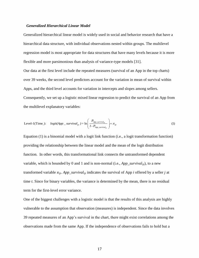
Generalized Hierarchical Linear Model
Generalized hierarchical linear model is widely used in social and behavior research that have a
hierarchical data structure, with individual observations nested within groups. The multilevel
regression model is most appropriate for data structures that have many levels because it is more
flexible and more parsimonious than analysis of variance-type models [31].
Our data at the first level include the repeated measures (survival of an App in the top charts)
over 39 weeks, the second level predictors account for the variation in mean of survival within
Apps, and the third level accounts for variation in intercepts and slopes among sellers.
Consequently, we set up a logistic mixed linear regression to predict the survival of an App from
the multilevel explanatory variables:
tLevel-1(Time ): _ ln (1)ijt
ijt
App_survival
ijt ijt
App_survival
Plogit(App survival )=
1- P
Equation (1) is a binomial model with a logit link function (i.e., a logit transformation function)
providing the relationship between the linear model and the mean of the logit distribution
function. In other words, this transformational link connects the untransformed dependent
variable, which is bounded by 0 and 1 and is non-normal (i.e., App_survivalijt), to a new
transformed variable πijt. App_survivalijt indicates the survival of App i offered by a seller j at
time t. Since for binary variables, the variance is determined by the mean, there is no residual
term for the first-level error variance.
One of the biggest challenges with a logistic model is that the results of this analysis are highly
vulnerable to the assumption that observation (measures) is independent. Since the data involves
39 repeated measures of an App’s survival in the chart, there might exist correlations among the
observations made from the same App. If the independence of observations fails to hold but a

18
maximum likelihood logistic regression is used to estimate the standard errors of parameter
estimates one may conclude that something is significant when it actually is not. Thus, we
introduce a correlation structure among the repeated measures to account for correlations among
the events of an App. The correlation among the repeated observations made from the same App
(nested within an App) was assumed to be autoregressive. We assume that the current survival of
an App at t is influenced by predictors at t-1, autoregressive (1). Therefore this model
specification controls for whether an App is shown in the top chart in the last period.
The regression coefficient (πijt) varies across the App, and we model this variation with
predictors at the App level. Then, model for the (πijt) becomes:
i
5 6
Level-2 (App ) _ ) _ _
_ _ _ (2)
ijt 00j 01j ijt 02j ijt 03j ijt-1
04j ijt-1 0 j ijt 0 j ijt
0
: = + (App free_price + (App_minus initial_rank) + (App price_promotion)
+ (App quality_update) + (App popular_cate) + (App unpopular_cate)
7 8 9 0( _ ) ( _ _ ) _ _ _j ijt-1 0 j ijt-1 0 j ijt-1 ijApp review_avr + App log review_num + (App age of app) +
In equation (2), β00j and β0ij are the intercept and slopes for the regression equation used to
predict (πijt). τ0ij is error term for Appi and assumed to be normally distributed (i.e., mean of 0 and
variance of σ2τ). It accommodates un-modeled variability for the App-level part.
It is also desirable to construct a time-lagged dataset through which the impacts of App-level
explanatory variables on a subsequent survival event could be longitudinally assessed. Time-
varying variables at t-1 were used to examine whether an Appi is listed in the top chart at t. It
takes account of the effect of endogeneity (reverse causation) into the presented model.
Similarly, equation (3) includes seller-level predictor variables and accounts for variation among
sellers.
j 000 001 002 003 00
1 010 01 2 020 02 3 030 03
4 040 04 5 050 05 6 060
Level-3 (Seller ) : ( _ _ ) ( _ _ ) ( _ _ * _ )
; ;
; ;
00j jt-1 jt-1 jt-1 j
0 j j 0 j j 0 j j
0 j j 0 j j 0 j
Seller num app Seller num cate Seller num app num cate u
u u u
u u
06
7 070 07 8 080 08 9 090 09
(3)
; ;
j
0 j j 0 j j 0 j j
u
u u u

19
Equation (3) indicates that while seller-level predictors for App portfolio management only
influence the mean of App’s survival (β00), App-level predictors have unconditional random
intercepts (μ) and slopes (γ) at seller-level to examine how App-specific properties vary under
different sellers. Thus, we assume that App-specific decisions are not affected by variables at the
seller-level. The residual term of u00j accommodates the un-modeled variability at the seller-level.
Finally, substituting (2) and (3) into (1) yield a combined multilevel model as follows:
000
001 002 003
010 020 030
_
( _ _ ) ( _ _ ) ( _ _ * _ )
_ _ _
ijt
jt-1 jt-1 jt-1
ijt ijt ijt -1
logit(App survival )=
Seller num app Seller num cate Seller num apps num cate
+ (App free_price) + (App minus_initial_rank) + (App price_promotion)
040 050 060
070 080 090
0
01 02
_ _ _
( _ ) ( _ ) _ _ _ (4)
_
ijt -1 ijt ijt
ijt -1 ijt-1 ijt-1
ij
j ijt j
+ (App quality_update) + (App popular_cate) (App unpopular_cate)
App review_avr + App review_num + (App age of app)
+
u (App free_price) + u (
03
04 05 06
07 08 0
_ _
_ _ _
( _ ) ( _ )
ijt j ijt -1
j ijt-1 j ijt j ijt
j ijt -1 j ijt-1
App minus_initial_rank) + u (App price_promotion)
u (App quality_update) u (App popular_cate) u (App unpopular_cate)
u App review_avr u App log_review_avr u
90
00
_ _ _j ijt -1
j
(App age of app)
u
The combined equation shows the single mixed-model equation and reveals that our model has
13 fixed effects (coefficients of ϒ) and 11 random effects (coefficients of μ and τ). Notice that
there is no cross-level interaction effect, because seller-level predictors are allowed to affect only
the intercept in Level-2.
Hazard Model
We measure the impact of a seller’s product portfolio strategy and App-level properties on Apps’
and sellers’ survival times in the charts by using a set of hazard models. Traditional survival
analysis approaches assume homogenous populations and the same hazard of having an event for
individuals. Consequently, they do not account for the problem of dependence caused by
unobserved heterogeneity [58]. Thus, the standard errors may become too small, and may
subsequently lead to misleading significance of estimates and high p-values [1]. Therefore, we

20
conduct the survival analysis of nested data, and use a frailty term to account for unobserved
heterogeneity at seller level. We utilize four distinct hazard models. The first two models are
Cox semi-parametric models, and the other two are parametric models with Weibull and logit
functions.
A Cox proportional hazards (PH) model assesses the relationship of predictor variables to
survival time t of App i. Cox PH model allows us to handle both continuous and categorical
variables and to estimate the parameters for each covariate without specifying the baseline
hazard [23].
The first model is a reference model that examines the net effect of each explanatory variable on
the hazard function to measure the App’s survival in the chart. The hazard function of App in the
top 300 is presented as:
hi(t | Xj, Zij) = exp(βXj + δZij) ∙ h0 (t) (5)
_ _
_ _ _
_ _
_ _ _ _
, _ _ _ _
_ _ * _ _ _
ij
ij
ij
j ij
j j i j ij
j j i
App free price
App minus initial rank
App price promotion
Seller num app App quality update
where X Seller num cate and Z App popular cate
Seller num app num cate App unpopular cate
_ _
_ _ _
_ _ _
j
ij
ij
ij
App review avr
App log review num
App age of app
h0(t) is a non-parametric baseline hazard, and Xj and Zij are the vectors of the covariates for the
seller j and App i offered by seller j, β and δ are coefficients of the covariates estimated from
Maximum Partial Likelihood Estimates (MPLE) and it represents the effect of the covariates on
hazard rate. When the parameter estimate of an explanatory variable is positive (negative), we
can conclude that an App i’s hazard rate (or rates of exiting from the top charts) increases
(decreases) with the variable.
The second model is a Cox model with a frailty term. It examines how Apps’ survivals in the top

21
charts vary at the seller level. The hazard rate for Cox model with frailty is as follows:
hi(t | Xj, Zij) = exp(βXj + δZij) ∙ rj∙ h0(t) (6)
rj represents the random (frailty) term for a seller j who offers individual App i. The frailty
components of rj are assumed to be distributed as gamma with mean one and an unknown
variance θ [2, 30, 34]. The penalized partial likelihood approach was used for fitting the frailty
model [50]. Since the baseline hazard for the first two models is not specified (i.e., non-
parametric baseline hazard) and the true underlying model is not given, we introduce two
parametric hazard models (a Weibull random-effects hazard model and a discrete-time logit
random-effects hazard model) with frailty to check if the frailty term in a Cox frailty model (i.e.,
the third model) is significant. The random terms in the Weibull hazard model and the discrete-
time logit model are assumed to follow the gamma distribution [43] and the normal distribution
[1] respectively. For a hazard model, the inclusion of time-varying variables can introduce
endogeneity [10, 11, 37]. Endogenous time-varying covariates cause bias in coefficient estimates
[33]. Since our hazard models include both time-independent (e.g., App_free_price,
App_popular cate, and App_minus_initial_rank) and time-varying (e.g., Seller_num_app,
Seller_num_cate, and App_review_num) covariates, the estimates from those time-dependent
covariates are subject to the effect of endogeneity.
Goodliffe [33] suggested a set of approaches that fix the problem of endogenous time-varying
covariates in a hazard model based on relevant prior literature: (1) drop the covariate only; (2)
ignore the problem [6]; (3) jointly model the duration and the time varying covariate [24]; (4) use
the ideas of simultaneous equations to duration models [7]; (5) include the covariate, but drop the
time-varying portion [33]. While the first four approaches have statistical problems of omitted
variables, bias in coefficient estimates, complexity in modeling, and difficulty in finding a true

22
instrument, the fifth approach works best by “taking away the part of the covariate that is mostly
likely to be tainted by reverse causation” [33]. In line with his suggestion, we used the time-
invariant explanatory variables. In other words, we used the averaged values of time-dependent
covariates (e.g., averaged review score and review number) over an App’s survival duration and
introduced dummies for time-varying variables such as App_price_promotion and
App_quality_update (i.e., if an App’s quality indicators / price were changed at least once), and
ignore the changes in those covariates. This approach resulted in no major changes to parameter
estimates and therefore we conclude that endogeneity bias is not likely impacting our results.
Count Regression Model
In order to reexamine the main results from GHLM, we have run a pooled count regression
model for individual sellers across 39 weeks. One-week time lag is used for estimating
associations between seller-level explanatory variables at t-1 (Xjt-1) and a seller’s number of Apps
in the top chart at t, Seller_num_apps_topjt.
E [Seller_num_app_topjt | Xjt-1] = βX jt-1 + εj (7)
The two supplemental models have some potential limitations for fitting the data into a
multilevel framework. The hazard model censors Apps not having continuous durations over the
study period (55% of the Apps were censored). Hierarchical survival analysis approach has not
been well established due to its complex estimation procedure where the solutions are not usually
expressed in closed form [51]. With GHLM, it is possible to utilize a discrete survival time
approach, in which the survival to an event at a discrete time is a binary dependent variable, and
incorporate hierarchical structure in the data [1].

23
Since the dependent variable of a count regression model is numbers of Apps in the charts of
individual seller, the model does not include App-level explanatory variables, and so the App-
specific properties that may affect the sales performance are ignored in the modeling setting. In
the GHLM, since the survival time of a seller in the top chart does not consider the presence of
multiple Apps in the top chart, the seller’s exact sales performance in a specific period may not
be taken into account. The count regression model allows us to examine how a seller’s
assortment of Apps across various categories affects the total number of Apps in the top charts.
Results
The results from fitting a generalized hierarchical linear model appear in Table 3. While we have
not reported the correlation matrix, we did not find any strong correlations between explanatory
variables; the highest correlation (ρ=-.350) among explanatory variables is between
App_minus_initial_rank and App_price_promotion. Further, we tested for the presence of
multicollinearity by means of Variance Influence Factors (VIF) of each explanatory variable.
The largest VIF was below 2.0, which indicates that multicollinearity was not a problem in the
models.
In order to examine model explanation power due to the addition of random and fixed
explanatory variables, we sequentially ran Model I in five iterations. Model I(0) is a confound
logistic regression model that included all predictor variables without controlling cross-level
interactions. As a baseline (null) model, Model I(1) includes an unconditional intercept only.
Model I(2) and Model I(3) incorporate level-2 and level-3 fixed and random effects respectively.
Finally, Model I(4) combines all fixed and random effects across Level-2 and Level-3.
The ability of a model to predict better than a baseline model was used as an index of Goodness
of Fit. In hierarchical linear model, the deviance test is mostly used to compare the fixed and
random effects of competing models [44]. Improvements in predictability were determined by
the proportional reduction of deviance compared with the null (baseline) model [16].
24
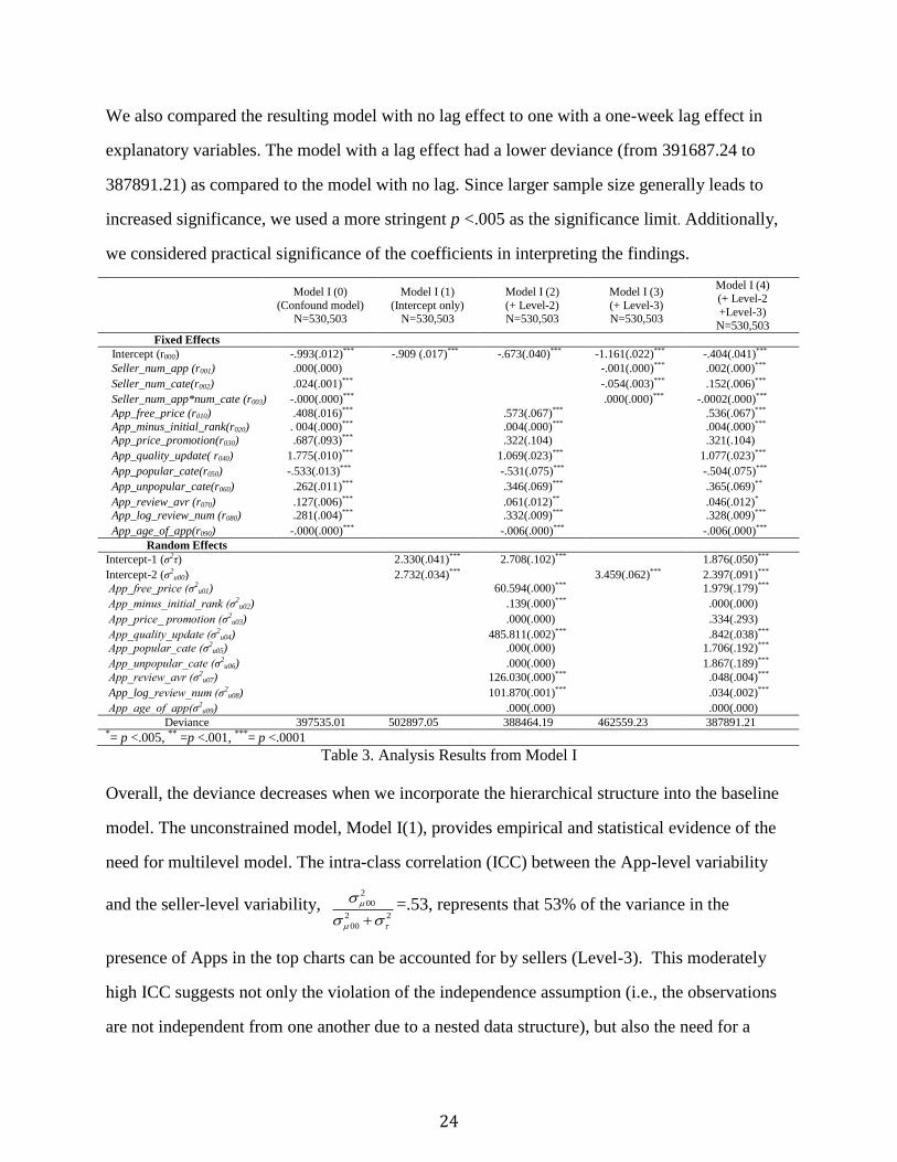
We also compared the resulting model with no lag effect to one with a one-week lag effect in
explanatory variables. The model with a lag effect had a lower deviance (from 391687.24 to
387891.21) as compared to the model with no lag. Since larger sample size generally leads to
increased significance, we used a more stringent p <.005 as the significance limit. Additionally,
we considered practical significance of the coefficients in interpreting the findings.
Model I (0)
(Confound model) N=530,503
Model I (1)
(Intercept only) N=530,503
Model I (2)
(+ Level-2) N=530,503
Model I (3)
(+ Level-3) N=530,503
Model I (4) (+ Level-2
+Level-3)
N=530,503
Fixed Effects
Intercept (r000) -.993(.012)*** -.909 (.017)*** -.673(.040)*** -1.161(.022)*** -.404(.041)***
Seller_num_app (r001) .000(.000) -.001(.000)*** .002(.000)***
Seller_num_cate(r002) .024(.001)*** -.054(.003)*** .152(.006)***
Seller_num_app*num_cate (r003) -.000(.000)*** .000(.000)*** -.0002(.000)***
App_free_price (r010) .408(.016)*** .573(.067)*** .536(.067)***
App_minus_initial_rank(r020) . 004(.000)*** .004(.000)*** .004(.000)***
App_price_promotion(r030) .687(.093)*** .322(.104) .321(.104)
App_quality_update( r040) 1.775(.010)*** 1.069(.023)*** 1.077(.023)***
App_popular_cate(r050) -.533(.013)*** -.531(.075)*** -.504(.075)***
App_unpopular_cate(r060) .262(.011)*** .346(.069)*** .365(.069)**
App_review_avr (r070) .127(.006)*** .061(.012)** .046(.012)* App_log_review_num (r080) .281(.004)*** .332(.009)*** .328(.009)***
App_age_of_app(r090) -.000(.000)*** -.006(.000)*** -.006(.000)***
Random Effects
Intercept-1 (σ2τ) 2.330(.041)*** 2.708(.102)*** 1.876(.050)***
Intercept-2 (σ2u00) 2.732(.034)*** 3.459(.062)*** 2.397(.091)***
App_free_price (σ2u01) 60.594(.000)*** 1.979(.179)***
App_minus_initial_rank (σ2u02) .139(.000)*** .000(.000)
App_price_ promotion (σ2u03) .000(.000) .334(.293)
App_quality_update (σ2u04) 485.811(.002)*** .842(.038)***
App_popular_cate (σ2u05) .000(.000) 1.706(.192)***
App_unpopular_cate (σ2u06) .000(.000) 1.867(.189)***
App_review_avr (σ2u07) 126.030(.000)*** .048(.004)***
App_log_review_num (σ2u08) 101.870(.001)*** .034(.002)***
App_age_of_app(σ2u09) .000(.000) .000(.000)
Deviance 397535.01 502897.05 388464.19 462559.23 387891.21 *= p <.005, ** =p <.001, ***= p <.0001
Table 3. Analysis Results from Model I
Overall, the deviance decreases when we incorporate the hierarchical structure into the baseline
model. The unconstrained model, Model I(1), provides empirical and statistical evidence of the
need for multilevel model. The intra-class correlation (ICC) between the App-level variability
and the seller-level variability, 2
00
2 2
00
=.53, represents that 53% of the variance in the
presence of Apps in the top charts can be accounted for by sellers (Level-3). This moderately
high ICC suggests not only the violation of the independence assumption (i.e., the observations
are not independent from one another due to a nested data structure), but also the need for a

25
multilevel model incorporating seller-level properties [44].
Model I(2) explains the association between App-specific properties and an App’s success
consistent with our expectation. When only seller level variables are considered (Model I(3)),
coefficients of Seller_num_app and Seller_num_cate are negative, thus contradicting theoretical
prediction. This result indicates how a mis-specified multi-level model can lead to erroneous
conclusions [55]. It also shows the effect of number of Apps to be insignificant. However, the
deviance in this model was relatively high. Finally, the combined three-level Model I(4) allows
us to obtain the correct estimates by incorporating intra-class random effects with the lowest
deviance. The coefficient signs in Model I(4) confirm the theoretical predictions related to
portfolio characteristics in that the number of Apps and number of categories both improve
outcome. It clearly demonstrates the need to consider both sellers’ portfolio decisions and App
characteristics in sales performance measurement. However, a user’s unobservable self-selection
for buying an App, which is not controlled in this research setting, is also likely to affect the
success of App sales. For example, a user may purchase a paid App after trying its free version
[41]. In addition, strong ranking effects in the App markets could form a bias among users to
predominantly fixate on hit products [32], and subsequently, users may download the Apps in the
top charts.
Because this model specification assumes that seller-level explanatory variables are not
correlated with unobserved seller-level fixed properties in the error term, controlling for seller-
level heterogeneity is important. In the context of our study, however, it is difficult to identify
strong and valid instruments that are correlated with seller-level App assortment decisions. A
fixed effects modeling approach might be a technique to correct for such omitted variables at the
seller-level, but this is generally difficult to accomplish for a model with a nested data structure.
Inclusion of seller-level dummies for fixed effects will introduce the incidental parameters
problems [59]. We employed a conditional fixed effect logistic regression model to account for
26
seller-level fixed effects4. The estimation results showed that the signs and significance levels
across the models are qualitatively identical. Although the estimates of App-level estimates are
slightly different from that of GHLM, these differences are likely due to differing model
assumptions. It leads us to confirm that our estimates from GHLM on seller-level Apps portfolio
decisions are highly robust to an alternative model specification that handles seller-level
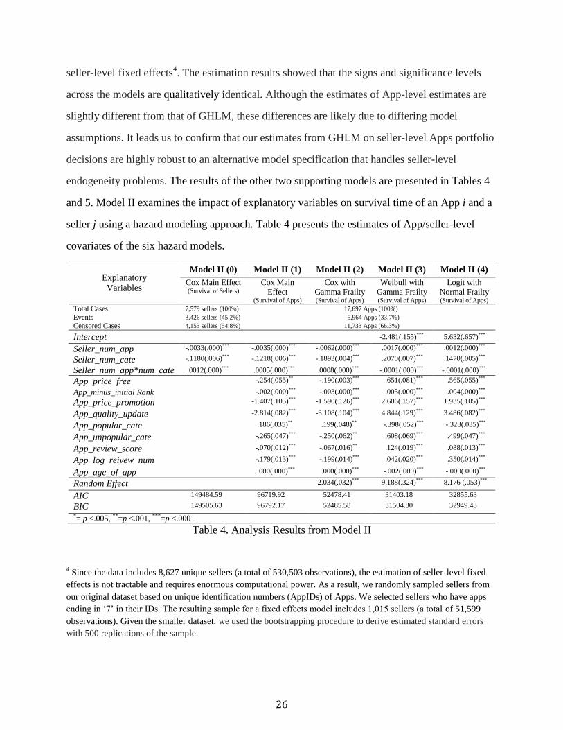
endogeneity problems. The results of the other two supporting models are presented in Tables 4
and 5. Model II examines the impact of explanatory variables on survival time of an App i and a
seller j using a hazard modeling approach. Table 4 presents the estimates of App/seller-level
covariates of the six hazard models.
Explanatory
Variables
Model II (0) Model II (1) Model II (2) Model II (3) Model II (4)
Cox Main Effect (Survival of Sellers)
Cox Main
Effect (Survival of Apps)
Cox with
Gamma Frailty (Survival of Apps)
Weibull with
Gamma Frailty (Survival of Apps)
Logit with
Normal Frailty (Survival of Apps)
Total Cases 7,579 sellers (100%) 17,697 Apps (100%) Events 3,426 sellers (45.2%) 5,964 Apps (33.7%) Censored Cases 4,153 sellers (54.8%) 11,733 Apps (66.3%)
Intercept -2.481(.155)*** 5.632(.657)***
Seller_num_app -.0033(.000)*** -.0035(.000)*** -.0062(.000)*** .0017(.000)*** .0012(.000)***
Seller_num_cate -.1180(.006)*** -.1218(.006)*** -.1893(.004)*** .2070(.007)*** .1470(.005)***
Seller_num_app*num_cate .0012(.000)*** .0005(.000)*** .0008(.000)*** -.0001(.000)*** -.0001(.000)***
App_price_free -.254(.055)** -.190(.003)*** .651(.081)*** .565(.055)***
App_minus_initial Rank -.002(.000)*** -.003(.000)*** .005(.000)*** .004(.000)***
App_price_promotion -1.407(.105)*** -1.590(.126)*** 2.606(.157)*** 1.935(.105)***
App_quality_update -2.814(.082)*** -3.108(.104)*** 4.844(.129)*** 3.486(.082)***
App_popular_cate .186(.035)** .199(.048)** -.398(.052)*** -.328(.035)***
App_unpopular_cate -.265(.047)*** -.250(.062)** .608(.069)*** .499(.047)***
App_review_score -.070(.012)*** -.067(.016)** .124(.019)*** .088(.013)***
App_log_reivew_num -.179(.013)*** -.199(.014)*** .042(.020)*** .350(.014)***
App_age_of_app .000(.000)*** .000(.000)*** -.002(.000)*** -.000(.000)***
Random Effect 2.034(.032)*** 9.188(.324)*** 8.176 (.053)***
AIC 149484.59 96719.92 52478.41 31403.18 32855.63
BIC 149505.63 96792.17 52485.58 31504.80 32949.43
*= p <.005, **=p <.001, ***=p <.0001
Table 4. Analysis Results from Model II
4 Since the data includes 8,627 unique sellers (a total of 530,503 observations), the estimation of seller-level fixed
effects is not tractable and requires enormous computational power. As a result, we randomly sampled sellers from
our original dataset based on unique identification numbers (AppIDs) of Apps. We selected sellers who have apps
ending in ‘7’ in their IDs. The resulting sample for a fixed effects model includes 1,015 sellers (a total of 51,599
observations). Given the smaller dataset, we used the bootstrapping procedure to derive estimated standard errors
with 500 replications of the sample.
27
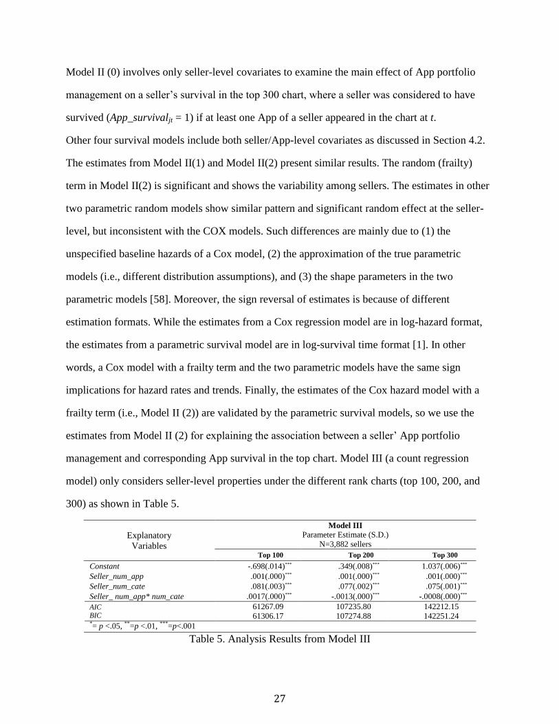
Model II (0) involves only seller-level covariates to examine the main effect of App portfolio
management on a seller’s survival in the top 300 chart, where a seller was considered to have
survived (App_survivaljt = 1) if at least one App of a seller appeared in the chart at t.
Other four survival models include both seller/App-level covariates as discussed in Section 4.2.
The estimates from Model II(1) and Model II(2) present similar results. The random (frailty)
term in Model II(2) is significant and shows the variability among sellers. The estimates in other
two parametric random models show similar pattern and significant random effect at the seller-
level, but inconsistent with the COX models. Such differences are mainly due to (1) the
unspecified baseline hazards of a Cox model, (2) the approximation of the true parametric
models (i.e., different distribution assumptions), and (3) the shape parameters in the two
parametric models [58]. Moreover, the sign reversal of estimates is because of different
estimation formats. While the estimates from a Cox regression model are in log-hazard format,
the estimates from a parametric survival model are in log-survival time format [1]. In other
words, a Cox model with a frailty term and the two parametric models have the same sign
implications for hazard rates and trends. Finally, the estimates of the Cox hazard model with a
frailty term (i.e., Model II (2)) are validated by the parametric survival models, so we use the
estimates from Model II (2) for explaining the association between a seller’ App portfolio
management and corresponding App survival in the top chart. Model III (a count regression
model) only considers seller-level properties under the different rank charts (top 100, 200, and
300) as shown in Table 5.
Explanatory
Variables
Model III
Parameter Estimate (S.D.)
N=3,882 sellers
Top 100 Top 200 Top 300
Constant -.698(.014)*** .349(.008)*** 1.037(.006)***
Seller_num_app .001(.000)*** .001(.000)*** .001(.000)***
Seller_num_cate .081(.003)*** .077(.002)*** .075(.001)***
Seller_ num_app* num_cate .0017(.000)*** -.0013(.000)*** -.0008(.000)***
AIC BIC
61267.09
61306.17
107235.80
107274.88
142212.15
142251.24 *= p <.05, **=p <.01, ***=p<.001
Table 5. Analysis Results from Model III
28
In Model III, the large ratio of deviance to degree of freedom (12.229) indicated the problem of
overdispersion. In other words, observed variance is greater than the mean since the mean of
Poisson distribution is equal to its variance. Although we expect the residual deviance / degree of
freedom to be approximately 1.0, the deviance is almost 10 times as large as the degree of
freedom. In order to adjust the problem of over-dispersion, we used a negative binomial
regression model. By allowing for more variability in the data, this approach accounted for over-
dispersion. Overall, the deviance / degree of freedom value is much closer to 1.0 than that in
Poisson regression model. As shown in Tables 4 and 5, the results from a Cox hazard model with
frailty and a count regression model support our findings in Model I.
Seller-level Properties (App Portfolio Management)
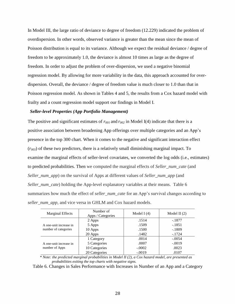
The positive and significant estimates of r001 and r002 in Model I(4) indicate that there is a
positive association between broadening App offerings over multiple categories and an App’s
presence in the top 300 chart. When it comes to the negative and significant interaction effect
(r003) of these two predictors, there is a relatively small diminishing marginal impact. To
examine the marginal effects of seller-level covariates, we converted the log odds (i.e., estimates)
to predicted probabilities. Then we computed the marginal effects of Seller_num_cate (and
Seller_num_app) on the survival of Apps at different values of Seller_num_app (and
Seller_num_cate) holding the App-level explanatory variables at their means. Table 6
summarizes how much the effect of seller_num_cate for an App’s survival changes according to
seller_num_app, and vice versa in GHLM and Cox hazard models.
Marginal Effects Number of
Apps / Categories Model I (4) Model II (2)
A one-unit increase in
number of categories
2 Apps .1514 -.1877
5 Apps .1509 -.1851
10 Apps .1500 -.1809
20 Apps .1482 -.1724
A one-unit increase in
number of Apps
1 Category .0014 -.0054
5 Categories .0007 -.0019
10 Categories -.0002 .0023
20 Categories -.0019 .0107
* Note: the predicted marginal probabilities in Model II (2), a Cox hazard model, are presented as
probabilities exiting the top charts with negative signs.
Table 6. Changes in Sales Performance with Increases in Number of an App and a Category
29
The predicted probabilities provide the changes in the probability of an App’s survival with a
one-unit increase in Seller_num_app or Seller_num_cate. Overall, the marginal effects are
largely stable at different numbers of Apps and categories. The marginal effects of adding a
category, ijt
ijt-1
Prob(App_survival = 1)
Seller_num_cate
, are positive at different numbers of Apps. The marginal effects
of adding an additional App, ijt
ijt-1
Prob(App_survival = 1)
Seller_num_app
, are much smaller than those of Sell_num_cate
and practically insignificant.
Overall, the results indicate that expanding across categories has greater practical significance to
sellers. The scope economy argument seems to therefore apply to the Apps market quite
significantly.
The hazard model also supports the positive association between broadening Apps over multiple
categories and successful App sales. The marginal effects of seller-level App portfolio decisions
in this case are expressed in terms of predicted probability of exiting the top charts. A one-unit
increase in seller_num_cate decreases an App’s probability of exit by 18.77% when a seller
offers the second App in a new category as compared to doing nothing.
Thus, sellers who provide Apps in various categories (i.e., diversify Apps over multiple
categories) and have larger variations in choosing categories (i.e., large selection of selling
categories) survive longer on the top charts and as a result have better sales performance. The
marginal effects remain stable as the number of Apps increase.
A look at some notable sellers supports this observation as well. Table 7 illustrates App vendors’
App portfolio management (number Apps/ categories) and their overall performance. While first
three sellers have lower overall sales performance and offer multiple Apps in a few categories,
other sellers have relatively higher sale performance with Apps diversified over various
30
categories. For instance, Iceberg Reader, an online media publisher, offers 6,049 Apps on
AppStore with only 6 categories, and has 55 Apps in the top 300 charts. Meanwhile, Oceanhouse
Media, an individual developer, has listed 49 of her 141 Apps in the top chart by selling Apps in
12 categories.
App Vendors Number of
Published Apps
Number of Selling
Categories
Number of Apps
in the Top 300
Overall Sales Performance
Number of Apps in the Top Charts
Total Number of Published Apps
Libriance Inc 1,038 1 1 .10%
Iceberg Reader 6,049 6 55 .91%
Deadly Dollar 53 1 4 7.55%
Oceanhouse Media 141 12 49 34.75%
SIS Software 17 10 6 35.29%
iHandy soft 22 5 8 36.36%
Table 7. App Portfolio Management and Sellers’ Sales Performance
App-level Properties
The estimates from App- and seller-level analysis in Model I and Model II present the
relationship between App-specific properties decided by a seller and an App’s survival periods in
the top chart. These results highlight the main features of Apps that help sellers to strategize their
Apps for better sales. To interpret a one-unit change in app-level covariates on the success of
Apps, we utilized odds ratios and hazard ratios of the estimates.
The estimate of App_free_price is positive in Model I(4), as expected, and strongly significant. It
indicates that free Apps are around 1.7 (=exp(.536)) times more likely to survive in the top charts
as compared to paid Apps. The estimate from Model II (2) also supports this finding. It suggests
that when Apps are offered free of charge, the hazard ratio decreases by 17.2% (=100*[1-exp(-
.1896)]) as compared to the paid Apps. Around 20% of top 300 Apps are free and most of them
are either lite-version of paid Apps or require additional payments (e.g., in-app purchases) for
more features (e.g., game money or network supports) when running Apps. Even most pure free
31
Apps retain advertising proceeds. That is, free Apps do not mean the absence of revenues. From
our observation around 8% of observed Apps in the top grossing 300 were offered for purely free.
Thus, as with other information goods contexts, free Apps create opportunities for larger network
of users [12] and increased demand in a complementary premium good [47].
Initial popularity is an important determinant of survival. The estimate of
App_Minus_initial_rank is positive and significant. However, the improvement due to initial
rank lacks practical significance (one rank higher at its first week increases the presence of an
App in the charts by nearly 0.4% in the models). The positive association of initial rank with
survival is consistent with the findings from prior studies with digital goods [52, 57, 60]. Thus,
there is limited evidence for returns to efforts on App advertising and promotion before release
[26].
Quality updates appear to have a bigger impact on App survival than price changes. In GHLM,
the estimate of App_price_promotion is not significant while that from the hazard model is
negative and significant. Apps that had offered at least one quality update (or promotional price)
during the study period increased the chance of survival in the top charts 2.9 (or 1.3) times as
compared to non-updated Apps, and lowered hazard rate of 95.5% (or 79.6%) than when they
made no updates. Moreover, these updates have differing impact based on seller. Even though
further studies on this issue are required, we empirically confirm that sellers can impact the
success of Apps by making targeted updates to price and quality in mobile App markets.
The estimates from App_popular_cate and App_unpopular_cate in Model I (4) indicate that
Apps offered in the popular categories have relatively lower odds of survival and shorter survival
periods as compared to those in unpopular categories. In Model II (2), the estimated risk of
exiting the top chart increases 1.22 times if an App is offered in the popular categories. Therefore,
32
from the literature on long tail effects [13, 29], we can divide categories into popular-App
categories (head) and niche-App categories (tail) based on their popularity in the AppStore
market. Even though the Apps offered in the popular categories may have more downloads, they
could have shorter periods in the top charts since these Apps would compete with numerous
popular Apps. For instance, around 716 Apps are released a day and 40% of them are provided
in the popular categories (i.e., Games, Books, and Entertainments). It implies that there exists
severe competition among sellers and impacts survival in top charts.5
Finally, Apps that gained higher volume and higher review scores have higher success and lower
hazard ratios. As evidenced in prior literature, positive user reviews have the potential to increase
product demand [27, 42] Similarly, Apps offered by reputable sellers, who have overall higher
average user review scores across their Apps in the top 300, have lower hazard rates, but the
volume of reviews does not influence App’s survival time. These results reveal that existing
users’ satisfaction from Apps can bring about new user interests to the Apps. Furthermore, we
can argue that users tend to trust (purchase) Apps offered by reputable sellers who had good
review scores associated with other Apps.
Sensitivity and Robustness Analysis
Our main results are restricted to the probability of an App’s survival in the top 300 charts. We
conducted three different post-hoc analyses with GHLM to test the sensitivity and validity of our
model.
5 We also tested if different combination of (un)popular categories have the same results. The most / least popular
categories (Game vs. Weather) and the four most/least popular ones (Game, Book, Entertainment, Lifestyle vs.
Medical, Navigation, Weather, Finance) were selected into the analyses. The results present that the different
selections of categories do not change the sign and significance of estimates from our original selection. Also, these
selections do not significantly change other estimates as well.
33
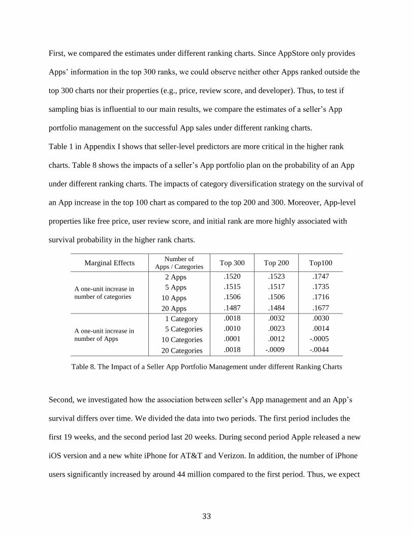
First, we compared the estimates under different ranking charts. Since AppStore only provides
Apps’ information in the top 300 ranks, we could observe neither other Apps ranked outside the
top 300 charts nor their properties (e.g., price, review score, and developer). Thus, to test if
sampling bias is influential to our main results, we compare the estimates of a seller’s App
portfolio management on the successful App sales under different ranking charts.
Table 1 in Appendix I shows that seller-level predictors are more critical in the higher rank
charts. Table 8 shows the impacts of a seller’s App portfolio plan on the probability of an App
under different ranking charts. The impacts of category diversification strategy on the survival of
an App increase in the top 100 chart as compared to the top 200 and 300. Moreover, App-level
properties like free price, user review score, and initial rank are more highly associated with
survival probability in the higher rank charts.
Marginal Effects Number of
Apps / Categories Top 300 Top 200 Top100
A one-unit increase in
number of categories
2 Apps .1520 .1523 .1747
5 Apps .1515 .1517 .1735
10 Apps .1506 .1506 .1716
20 Apps .1487 .1484 .1677
A one-unit increase in
number of Apps
1 Category .0018 .0032 .0030
5 Categories .0010 .0023 .0014
10 Categories .0001 .0012 -.0005
20 Categories .0018 -.0009 -.0044
Table 8. The Impact of a Seller App Portfolio Management under different Ranking Charts
Second, we investigated how the association between seller’s App management and an App’s
survival differs over time. We divided the data into two periods. The first period includes the
first 19 weeks, and the second period last 20 weeks. During second period Apple released a new
iOS version and a new white iPhone for AT&T and Verizon. In addition, the number of iPhone
users significantly increased by around 44 million compared to the first period. Thus, we expect
34
more severe competition among sellers (or developers) in the second period. The estimates are
presented in Table 2 in Appendix I. Since we used time-varying explanatory variables in GHLM,
the negative intercept terms indicate the overall decrease of App survival (i.e., the mean of
survival when all of explanatory variables take on the value zero) in the second period.
Furthermore, the seller-level decisions play more important role in the second period.
Marginal Effects Number of
Apps / Categories
Period I
(Week 1 ~ 19)
Period II
(Week 20~39)
A one-unit increase in
number of categories
2 Apps .1446 .1685
5 Apps .1444 .1682
10 Apps .1441 .1678
20 Apps .1434 .1668
A one-unit increase in
number of Apps
1 Category .0013 .0066
5 Categories .0010 .0062
10 Categories .0007 .0057
20 Categories .0000 .0048
Table 9. The Impacts of Increases in Number of an App and a Category
Finally, we also incorporated App users’ hedonic and utilitarian uses of Apps into the model. By
adding a hedonic dummy (coded “1” if an App is offered in hedonic categories6 and coded “0” if
an App is offered in utilitarian categories), we looked for the association between App’s hedonic
or utilitarian uses and Apps’ survival. In the first model, we included a hedonic dummy instead
of (un) popular dummies, and in the second model both category-related variables were added
(see Table 3 in Appendix I). The results show that the estimate of a hedonic dummy is not
significant in both models and Goodness of Fit worsened. Since App_popular_cate (games,
books, and entertainment) and App_unpopular_cate (medical, navigation, and weather), in
6 - Hedonic Categories: Book, Entertainment, Games, Healthcare-fitness, Lifestyle, Music, Navigation, News,
Photography, Social-networking, Sports, and Travel
- Utilitarian Categories: Business, Education, Finance, Medical, Productivity, Reference, Utilities, and Weather

35
general, reflect the hedonic and utilitarian Apps, our main model incorporated competitive
pressures adequately. Consequently, the results from sensitivity and robustness analysis give us
more confidence in the proposed empirical models.
Conclusion
Our findings demonstrate how mobile App seller product portfolio is associated with sales
performance. Specifically, diversification across selling categories is a key determinant of high
survival probability in the top charts and contributes to sales performance. Furthermore, we find
that offering free Apps, higher initial popularity, investment in less popular categories,
continuous updates on App features and price, and higher user feedbacks on Apps are positively
associated with sales performance. Therefore, these App-level attributes lead to further potential
user demand and increase the longevity of Apps.
Contribution and Managerial Implications
The results of this study have several significant implications to extant literature on digital
product management and business practice. From an academic perspective, our research creates
new knowledge about mobile App seller’s strategic decisions on product portfolio management
and its impact on success in mobile App markets. Our findings firmly establish the importance of
scope economies as an ingredient for success in mobile App market. Survival and sales
performance was greatly higher for sellers when participating across multiple categories than
otherwise. We also find that product price and quality upgrades are quite important in mobile
Apps market contexts. Prior studies in software management have been restricted to cost
reduction in software upgrades: optimal frequency of security patch updates [18] and the
expected time to perform major upgrade to software systems [38]. However, developers in App
36
markets can easily change price and features with lower costs and efforts than in traditional
software markets. It appears that the opportunity for frequent changes should indeed be exploited.
Limitations and Future Research Directions
The findings of this study are based on the survival of Apps only over 39 weeks in the top 300
chart. We continue to track and monitor the Apps to examine if there are reasons to expect
different results over a longer duration. The analytic approach used in the study does not allow
us to make causal predictions. Future research can examine the causal linkage between product
portfolio decisions and App performance. In addition, appearing in the top charts itself may have
a potential to facilitate purchase decision making at the point users initially search for Apps.
However, data availability restrictions prevent us from such App users’ potential preferential
attachment mechanisms. Furthermore, we estimated the sales amount of an App (or a seller)
with survival in the top charts and total number of Apps in the chart. However, there may exist
several alternatives to estimate actual sales amount instead of ranking. We also did not
specifically examine App specific features or seller specific characteristics. Further examination
of these attributes will be necessary in developing deep insights into mobile App markets.
While this study only considers a seller (or a developer) as a decision maker for App portfolio
management, many individual sellers provide Apps through big mobile software publishers such
as Gameloft or Chillingo. Thus, for such big publishers, the management of various developers
and much larger selections of mobiles Apps could be crucial for successful sales performance. In
the regard, it is important to investigate how publisher-level properties affect App-/seller-level
variables.
The results in this study are based on sellers in a single mobile App market. A seller’s mobile
App portfolio management and its impact on sales performance can vary under distinct App

37
market structures. For example, each market has a different number of categories (e.g., Apple: 20
categories; Blackberry: 18 categories; Google: 34 categories) and a different proportion of free
Apps (Apple: 25 percent; Google: 57 percent). As a result, future studies exploring sellers’
portfolio management in different mobile App markets and potential for platform competition
among the markets are necessary.
38
Reference
1. Allison, P.D. Survival Analysis using SAS: A Practical Guide. 2nd
Edition, Cary, NC: SAS
Institute Inc. 2010.
2. Andersen, P. K., Klein, J. P., Knudsen, K. M., and Palacios, R. T. Estimation of variance in
Cox's regression model with shared gamma frailties. Biometrics, 53, 4 (1997), 1475-1484.
3. Anderson, C. The Long Tail: Why the Future of Business is Selling Less of More. New York:
Hyperion, 2006.
4. Aribarg, A. and Arora, N. Inter-brand variant overlap: impact on brand preference and
portfolio profit. Marketing Science, 27, 3 (2008), 474-491.
5. Babin, B. J., Darden, W. R., and Griffin, M. Work and/or fun: Measuring hedonic and
utilitarian shopping value. Journal of Consumer Research, 20, 4 (1994), 644–656.
6. Bartels, L.M. Alternative misspecifications in a simultaneous-equation models, Political
Methodology, 11, 3/4 (1985), 181-199.
7. Bartels, L.M. Instrumental and quasi-instrumental variables. American Journal of Political
Science, 35, 3 (1991), 777-800.
8. Bailey E.E. and Friedlaender A.F. Market structure and multiproduct industries. Journal of
Economic Literature, 20, 3 (1982), 1024-1048.
9. Baumol, W., Panzar, J., and Willig R. Contestable markets and the theory of industry
structure. Harcourt Brace Jovanovich, New York: Harcourt College Publisher, 1982.
10. Bennett, D.S. 1999. Parametric models, duration dependence, and time-varying data
revisited. American Journal of Political Science, 43, 1 (1999), 256-270.
11. Bennett, D.S. and Stam, A.C. The duration of interstate wars, 1816-1985. American Political
Science Review, 90, 2 (1996), 239-257.
39
12. Bhargava, H. and Choudhary, V. Economics of an information intermediary with aggregation
benefits. Information Systems Research, 15, 1 (2004), 22-36.
13. Brynjolfsson, E., Hu, Y., and Smith, M. D. From niches to riches: The anatomy of the long
tail. Sloan Management Review, 47, 4 (2006), 67–71.
14. Brynjoffson, E., Hu, Y., and Smith, M.D. Long Tails vs. Superstars: The effect of
information technology on product variety and sales concentration patterns. Information
Systems Research, 21, 4 (2010), 736-747.
15. Brynjolfsson, E., Hu, Y., and Smith M.D. The longer tail: the changing shape of Amazon’s
sales distribution curve. working paper, SSRN, 2010.
16. Bryk, A.S. and Raudenbush, S.W. Hierarchical linear models: Applications and data analysis
methods. Newbury Park: Sage Publication, 1992.
17. Cardozo, R. and Smith, D. Applying financial portfolio theory to product portfolio decisions:
an empirical study source. The Journal of Marketing, 47, 2 (1983), 110-119.
18. Cavusoglu, H., Cavusoglu, H., and Zhang, J. Economics of security patch management,
Proceedings of the Fifth Workshop on the Economics of Information Security (WEIS),
University of Cambridge, England, 2006.
19. Chevalier, J. and Goolsbee, A. Measuring prices and price competition online: Amazon.com
and Barnes and Noble.com. Quantitative Marketing and Economics, 1, 2 (2003), 203-222.
20. Childers, T. L., Carr, C. L., Peck, J., and Carson, S. Hedonic and utilitarian motivations for
online retail shopping behavior. Journal of Retailing, 77, 4 (2001), 511–535.
21. Cooper, R.G. Industrial firms’ new product strategy. Journal of Business Research, 13, 2
(1985), 107-121.
40
22. Cottrell, T. and Nault, B. R. Product Variety and Firm Survival in the Microcomputer
Software Industry. Strategic Management Journal, 25, 10 (2004) 1005-1025.
23. Cox, D. R. Regression models and life-tables. Journal of the Royal Statistical Society, Series
B, 34, 2 (1972) 187-220
24. Cox, D.R. and Lewis, P.A.W. Multivariate point processes. Proceedings of the Sixth Berkeley
Symposium on Mathematical Statistics and Probability. Berkeley: University of California
Press, 3 (1972). 401-448.
25. Day, G.S. Diagnosing the Product Portfolio, Journal of Marketing. 4, 2 (1977), 29–38.
26. Dellarocas, C., Gao, G., and Narayan, R. Are consumers more likely to contribute online
reviews for hit or niche products? Journal of Management Information Systems, 27, 2 (2010),
127-158.
27. Dellarocas, C., Zhang, X, and Awad, N. F. Exploring the value of online product ratings in
revenue forecasting: The case of motion pictures. Journal of Interactive Marketing, 21, 4
(2007), 23-45.
28. Devinney, T. and Stewart, D. Rethinking the product portfolio: A generalized investment
model. Management Science, 34, 9 (1988), 1080-1095.
29. Elberse, A. Should you invest in the long tail?. Harvard Business Review, 86 (2008), 88–96.
30. Fan, J. and Li, R. Variable selection for Cox's proportional hazards model and frailty
model. The Annals of Statistics, 30, 1 (2002), 74-99.
31. Frees, E.W. Longitudinal and panel data analysis and applications in the Social Sciences.
New York: Cambridge University Press, 2004.
41
32. Ghose, A., Goldfarb, A., and Han, S. P. How is the Mobile Internet Different? Search Costs
and Local Activities. Information Systems Research, Articles in advance, 24, 3 (2013), 613-
631.
33. Goodliffe, J. The hazards of time-varying covariates. Proceeding of the annual meeting of
the American Political Science Association, Philadelphia, PA, 2003.
34. Gutierrez, R.G. Parametric frailty and shared frailty survival models. Stata Journal, 2, 1
(2002), 22-44.
35. Hartman, J. B., Shim, S., Barber, B., and O’Brien, M. Adolescents’ utilitarian and hedonic
web- consumption behavior: Hierarchical influence of personal values and innovativeness.
Psychology and Marketing, 23, 10 (2006), 813–839.
36. Hinz, O., Eckert, J., and Skiera, B. Drivers of the long tail phenomenon: an empirical
analysis. Journal of management information systems, 27, 4 (2011), 43-70.
37. Kalbáeisch, J.D. and Prentice, R.L. The statistical analysis of failure time data. 2nd
Edition,
New York: John Wiley & Sons, 2002.
38. Krishnan, M., Mukhopadhyay, C., and Kriebel, H. A decision model for software
maintenance. Information System Research, 15, 4 (2004), 396-412.
39. Lancaster, K. Variety, equity, and efficiency. New York: Columbia University Press, 1979.
40. Lee, G.W. and Raghu, T. S. Product portfolio and mobile apps success: evidence from App
store market. Proceedings of the 17th Americas Conference on Information Systems 2011,
Detroit, Michigan, 2011.
41. Lee, Y. and Tan, Y. Effects of different types of free trials and ratings in sampling of
consumer software: an empirical study. Journal of Management Information Systems, 30, 3
(2013), 213-246.
42
42. Li, X., Hitt, L., and Zhang, Z. Product reviews and competition in markets for repeat
purchase products. Journal of Management Information Systems, 27, 4 (2011), 9-42.
43. Liu, X. Survival Analysis: Models and Applications, 1st Edition, Chichester, UK John Wiley
& Sons, Ltd, 2012.
44. Luke, S. Multilevel modeling: quantitative applications in the social sciences, no. 143.
Thousand Oaks, CA: Sage Publications, 2004.
45. Oakes, D. Survival analysis. Journal of the American Statistical Association, 95, 449 (2000),
282-285.
46. Oestreicher-Singer, G. and Sundrarajan. Recommendation networks and the long tail of
electronic commerce. Working paper, New York University, New York. 2010.
47. Parker G. and Alstyne, M. V. Two-sided network effects: A theory of information product
Design, Management Science, 15, 10 (2005), 1494-1504.
48. Panzar J.C. and Willig R.D. Economies of scope. The American Economic Review, 71, 2
(1981), 268-272.
49. Quelch.J, and Kenny, D. Extend profits, not product lines. Harvard Business Review, (1994),
153-160.
50. Ripatti, S. and Palmgren, J. Estimation of multivariate frailty models using penalized partial
likelihood. Biometrics, 56, 4 (2000), 1016-1022.
51. Rodriguez, G. and Goldman, N. An assessment of estimation procedures for multilevel
models with binary responses. Journal of the Royal Statistical Society, 158, 1 (1995), 73-89.
52. Ronald, S. and Burt. Social contagion and innovation: cohesion versus structural equivalence.
American Journal of Sociology, 92, 6 (1987), 1287-1335.
43
53. Rothaermel, F., Hitt, M., and Jobe, L. Balancing vertical integration and strategic
outsourcing: effects on product portfolio, product success, and firm performance. Strategic
Management Journal, 27, 1 (2006), 1033-1056.
54. Sorenson, O. Letting the market work for you: an evolutionary perspective on product
strategy. Strategic Management Journal, 21, 5 (2000), 577-592.
55. Snijders, T. and Bosker, R. Multilevel analysis. London: Sage Publication, 1999.
56. Srinivasan, R., Lilien, G.L., and Rangaswamy, A. Survival of high tech firms: The effects of
diversity of product-market portfolios, patens, and trademarks. International Journal of
Research in Marketing, 25 (2008), 119-128.
57. Strobl, E. A. and Tucker, C. The dynamics of chart success in the U.K. pre-recorded popular
music industry. Journal of Cultural Economics, 24, (2000), 113-134.
58. Wong, J. H. How frail are Great British Immigrants to find first job after arrival? SAS Global
Forum 2012 paper, (2012), 1-5.
59. Wooldridge, J. Econometric Analysis of Cross Section and Panel Data. Boston: MIT Press,
2001.
60. Yamada, M. and Kato, H. A structural analysis of sales patterns of music CDs, INFORMS
Marketing Science Conference, Edmonton, Alberta, Canada, 2002.
44
Appendix I: Sensitivity Analysis
1. GHLM with Different Ranking Charts
Model 1
(Top 300)
Model 2
(Top 200)
Model 3
(Top 100)
Fixed Effects
Intercept (r000) -.404(.041)*** -.479(.040)*** -1.632(.050)***
Seller_num_app (r001) .002(.000)*** .003(.000)*** .004(.000)***
Seller_num_cate(r002) .152(.006)*** .153(.006)*** .175(.008)***
Seller_num_app*num_cate (r003) -.0002(.000)*** -.0002(.000)*** -.0004(.000)***
App_free_price (r010) .536(.067)*** .601(.067)*** .761(.093)***
App_minus_initial_rank(r020) .004(.000)*** .009(.000)*** .016(.000)***
App_price_ promotion (r030) .321(.104)* .357(.091)* .282(.089)
App_quality_update( r040) 1.077(.023)*** 1.077(.022)*** .922(.031)***
App_popular_cate(r050) -.504(.075)*** -.652(.075)*** -.774 (.099)***
App_unpopular_cate(r060) .365(.069)** .236(.071) .057(.085)
App_review_avr (r070) .046(.012)* .166 (.014)*** .238(.019)***
App_review_num (r080) .328(.009)*** .445(.010)*** .511 (.013)***
App_age_of_app(r090) -.006(.000)*** -.004(.000)*** -.003(.000)***
Random Effects
Intercept-1 (σ2τ) 1.876(.050)*** 1.987(.078)*** 1.920(.094)***
Intercept-2 (σ2u00) 2.397(.091)*** 2.330(.041)*** 2.184(.034)***
App_free_price (σ2u01) 1.979(.179)*** 1.72(.070)*** 2.623(.277)***
App_minus_initial_rank (σ2u05) .000(.000) .000(.000) .000(.000)
App_price_ promotion (σ2u03) .334(.293) .366(.211) .223(.173)
App_quality_update (σ2u02) .842(.038)*** .865(.040)*** 1.189 (.064)***
App_popular_cate (σ2u06) 1.706(.192)*** 1.440(.174)*** 1.665(.250)***
App_unpopular_cate (σ2u07) 1.867(.189)*** 1.800 (.185)*** 1.195(.202)***
App_review_avr (σ2u08) .048(.004)*** . 074(.006)*** .122(.009)***
App_log_review_num (σ2u09.) .034(.002)*** .044 (.003)*** .054(.004)***
App_age_of_app(σ2u10) .000(.000) .000(.000) .000(.000)
Deviance 387891.27 391771.08 388409.86
*= p <.005, **=p <.001, ***=p <.0001
Table 1. Analysis Results from Different Ranking Charts
45
2. GHLM with Two Periods
Period 1 (Week 1 ~ 19)
N=231,968
Period 2 (Week 20 ~ 39)
N=356,535
Fixed Effects
Intercept (r000) -1.307(.045)*** -1.619(.033)***
Seller_num_app (r001) .001(.000)*** .007(.000)**
Seller_num_cate(r002) .145(.008)*** . 168(.005)***
Seller_num_app*num_cate (r003) -.00006 (.000)** -.00009(.000)***
App_free_price (r010) .175(.065) .344(.078)**
App_minus_initial_rank(r050) .011(.000)*** . 004(.000)***
App_price_ promotion (r030) .028(.128) .695(.182)*
App_quality_update( r020) .759(.023)*** 1.917(.323)***
App_popular_cate(r060) -.339(.069)** -.529(.057)***
App_unpopular_cate(r070) .296(.059)** .294(.049)***
App_review_avr (r080) .017(.014) .026(.014)
App_review_num (r090) .204(.009)*** .261(.010)***
App_age_of_app(r0100) -.001(.000)*** -.001(.000)***
Random Effects
Intercept-1 (σ2τ) 1.274(.052)*** .890(.042)***
Intercept-2 (σ2u00) 2.003(.014)*** 1.388(.021)***
App_free_price (σ2u01) 1.005(.141)*** .648(.093)***
App_minus_initial_rank (σ2u05) .000(.000) .000(.000)
App_price_ promotion (σ2u03) .000(.000) 1.418(.571)
App_quality_update (σ2u02) .000(.000) 1.698(.076)***
App_popular_cate (σ2u06) .184(.155) .907(.132)***
App_unpopular_cate (σ2u07) .944(.124)*** .851(.106)***
App_review_avr (σ2u08) .037(.004)*** .024(.004)***
App_review_num (σ2u09.) .013(.002)*** .016(.002)***
App_age_of_app(σ2u10) .000(.000) .000(.000)
Deviance 152411.88 207329.54
*= p <.005, **=p <.001, ***=p <.0001
Table 2. Analysis Results from Different Periods
46
3. GHLM with a Hedonic / Utilitarian Variable
Model 1
( Hedonic Dummy only) N=530,503
Model 2
(+ Hedonic Dummy) N=530,503
Fixed Effects
Intercept (r000) -.442 (.017)*** -.385(.047)***
Seller_num_app (r001) .003(.000)*** .003(.000)***
Seller_num_cate(r002) .148(.006)*** .152(.006)***
Seller_num_app*num_cate (r003) -.0002(.000)*** -.0002(.000)***
App_free_price (r010) .579(.0682)*** .536(.068)***
App_minus_initial_rank(r020) .004(.000)*** .004 (.000)***
App_price_ promotion (r030) .306(.104) .312(.104)
App_quality_update( r040) 1.074(.021)*** 1.069(.0208)***
App_popular_cate(r050) . -.541(.047)**
App_unpopular_cate(r060) . .372(.071)***
App_review_avr (r070) -.046(.012)* .047(.012)*
App_review_num (r080) .325(.009)*** .326(009)***
App_age_of_app(r090) -.006(.000)*** -.003(.000)***
App_hedonic_cate(r0100) .033(.044) .111(.045)
Random Effects
Intercept-1 ( σ2τ) 2.438(.104)*** 2.229(.102)***
Intercept-2 (σ2u00) 2.732(.034)*** 3.363(.058)***
App_free_price (σ2u01) 2.101(.187)*** 2.017(.184)***
App_minus_initial_rank (σ2u02) .000(.000) .000(.000)
App_price_ promotion (σ2u03) .332(.294) .323(.292)
App_quality_update (σ2u04) .853(.038)*** .831(.038)***
App_popular_cate (σ2u05) . 1.678(.201)***
App_unpopular_cate (σ2u06) . 1.782(.197)***
App_review_avr (σ2u07) .047(.004)*** .047(.004)***
App_log_review_num (σ2u08.) .034(.002)*** .034(.002)***
App_age_of_app(σ2u09) .000(.000) .000(.000)
App_hedonic_cate(σ2u10) 1.518(.106)*** 1.318(.104)***
Deviance 396976.95 385245.89
*= p <.005, ** =p <.001, ***= p <.0001
Table 3. Analysis Results from Hedonic Use