No. 2013-02A

OFFICE OF ECONOMICS WORKING PAPER U.S. INTERNATIONAL TRADE COMMISSION

William Deese*

U.S. International Trade Commission

February 2013

*The author is with the Office of Economics of the U.S. International Trade Commission. Office of Economics working papers are the result of the ongoing professional research of USITC Staff and are solely meant to represent the opinions and professional research of individual authors. These papers are not meant to represent in any way the views of the U.S. International Trade Commission or any of its individual Commissioners. Working papers are circulated to promote the active exchange of ideas between USITC Staff and recognized experts outside the USITC, and to promote professional development of Office staff by encouraging outside professional critique of staff research.

Address correspondence to: Office of Economics

U.S. International Trade Commission Washington, DC 20436 USA

Determinants of Inbound Travel to the United States

Determinants of Inbound Travel to the United States

William Deese∗

February 6, 2013

Abstract

Travel and tourism services are among the largest globally traded services sectors.Data representing travelers to the United States from the 50 countries that contributedthe most inbound travelers between 1990 and 2010 were assembled. Income levels andreligion influenced which countries made it into the top 50 list. These data are thencombined with economic, policy, and cultural variables to estimate a demand model ofthese flows of travelers. These data contained substantial heterogeneity that traditionalpanel data methods do not adequately account for, and econometric methods that em-ploy a multi-factor error structure, such as those pioneered by Serlenga and Shin andothers, are used. These methods, which permit unobserved heterogeneous responses toglobal events, improved the statistical estimation and produced reasonable economicresults. Empirical results provide evidence that income, relative prices, cultural factors,and policies are major determinants of inbound U.S. travel. The Visa Waiver Programand a program that facilitates group travel by Chinese nationals had statistically sig-nificant positive effects on the numbers of inbound travelers. Being from a majorityEnglish-speaking country or a bordering country (Canada or Mexico) were the mostsignificant cultural or geographic factors.

∗The author is an economist at the U.S. International Trade Commission. This paper represents theviews of the author and is not meant to represent the views of the U.S. International Trade Commission orany of its commissioners.

1 Antecedents

Economic, policy, cultural, and geographic factors largely determine the source country

of inbound travelers to the United States each year. Relative prices and levels of income

are shown to be major influences on the numbers of inbound travelers. The Visa Waiver

Program and a program to facilitate group travel by Chinese nationals appear to increase

the flow of inbound travelers. Variables representing cultural identities and geography, such

as being from an English-speaking country or from Canada or Mexico, have a persistent

positive effect on numbers of travelers. Cultural and economic factors also determine the

countries that appear in the data used for this study, which consists of countries with the 50

largest flows of inbound U.S. travelers. These data contain substantial heterogeneity among

countries and over time, and recent techniques that permit a multi-factor error structure

improve the statistical estimation.

Transportation and travel-related services are the largest components of global services

trade and continue to grow, although other services sectors grew more rapidly between

2000 and 2010.1 The United States experienced similar trends. U.S. exports and imports of

travel services, passenger fares, and related services more than doubled between 1990 and

2010. However, travel services fell from 31 percent of total services exports in 1990 to 20

percent in 2010; similarly, imports of travel services fell from 38 percent of total services

imports in 1990 to 21 percent in 2010.2 In particular, U.S. trade in royalties and license fees,

insurance, and financial services, among others, grew more rapidly than travel and tourism.

In 2010, exports of travel services, valued at $104 billion, were the second largest single

industry category of U.S. services exports (after royalities and license fees). U.S. imports

of travel services in 2010 were the largest single industry category of services imports and

were valued at $76 billion.

Purchases of transportation and travel services by international travelers are important

1World Trade Organization, International Trade Statistics 2011, table III.2. The World Travel andTourism Council (WTTC) estimates that travel and tourism directly contributed 3 percent of global GDPin 2011 (WTTC, 2012, 3).

2Bureau of Economic Analysis, Survey of Current Business, various issues. The October issue usuallyhas data on services.

1

sources of economic activity in some areas. Expenditures by international travelers while in

the United States are counted as U.S. exports and directly contribute to U.S. employment.

Foreigners’ expenditures on locally produced goods and services may transform goods and

services that are not usually traded into traded goods.

The following section of this paper (part 2) reviews the related literature. Then, ge-

ographic, cultural, and policy factors (here collectively referred to as travel frictions) are

discussed in part 3. A demand model to explain flows of inbound travelers is developed

in part 4. The data on inbound tourism are explored in part 5, and a frictionless model

based solely on population is developed in part 6. The results of empirically estimating the

demand model using different econometric techniques are shown in part 7. Conclusions are

drawn in part 8.

2 Related Literature

This section reviews literature related to flows of travelers and demand for international

tourism services. These studies apply a fairly standard demand model to identify the

determinants of travel. Most of this work has focused on Australia and developing countries,

with only a few studies concentrating on the United States. However, an early article on

U.S. domestic travel begins the review because it addresses some key issues.

Long (1970) examined air passenger travel between the 13 largest U.S. cities during

1960–63 and assumed that people travel to shop, to conduct business, and to visit friends

and relatives. Curiously he did not consider other reasons, such as cultural activities or

recreation, but additional considerations may not have altered his model specification be-

cause data on the purpose of a trip were unavailable. He considered business and personal

travel to be proportional to the size of the destination and origin because economic and

personal relationships become more likely as the number of people increase. He included

a population variable to indicate numbers of personal and business trips. Relative prices

between the destination and origin and disposable income are important determinants of

2

shopping trips, and variables for cost-of-living indexes and per-capita income are included

to capture these ideas. The cost of transit is relevant for each type of travel. Lacking data

on transportation costs, he used distance between the origin and destination as a proxy.

The inclusion of variables for distance, population, and income make this model similar to

gravity models of trade flows. In fact, he estimated a pure gravity model with population

and distance as variables, and these variables alone explained much of the variation in flows

of air passengers. Parameter estimates for the price indexes and income were significant

however and improved the explanatory power of the model.

Keum (2010) modeled flows of business and leisure travelers between South Korea and

its 28 principal trading partners between 1990 and 2002 with a gravity model. In addition

to variables for distance and GDP, he included a regressor for economic similarity. He

estimated pooled and random effects models, but did not consider fixed effects. A test of

the pooled model revealed substantial heterogeneity among countries, and he rejected the

pooled model in favor of the random-effects model. The random-effects model took the

unobserved heterogeneity into account, but he did not test whether the random effects were

correlated with the regressors, and such correlation would call into question the validity

of the random-effects model. He found that the number of travelers between countries

increased with GDP and decreased with distance, but that the number of travelers did not

increase when two countries approach a more similar stage of development.3 He concluded

that distance was the single most important factor in explaining these travel flows, as

estimates of the parameters on the distance variable were the largest (in absolute value—

typically less than -1 depending upon the specification) and were significant at the 5 percent

level. Parameter estimates for GDP were also significant and typically less than 1.

Lim (1997) derived the basic demand model of travel flows as a function of income in the

originating country, transportation costs to the destination country, and price levels faced

by the traveler or tourist. This basic model does not have variables for prices of substitutes

and complements and applies the same variables regardless of the purpose of the trip. A

3This is known as the Linder hypothesis, after Linder who stated that trade increases as per-capita incomeand tastes converge. Linder, 1961.

3

number of articles apply variants of this basic model. For example, Lim and McAleer (2001)

examined the determinants of inbound tourism from Singapore to Australia using quarterly

data from 1980 to 1996. They estimated the basic demand model and found that real

income in Singapore and relative prices in the two countries were important determinants

of inbound tourism. They estimated an OLS model and found that income and price were

inelastic. They also estimated a cointegrated model, and airfare and exchange rates (a

proxy for price) were elastic in this version.

Divisekera (2003) examined demands for tourism among Australia, Japan, New Zealand,

the USA, and the UK, without including all combinations. He argued that regardless of

the purpose of the trip all tourists consume attributes of the destination along with other

available goods and services. Prices were weighted averages of tourism price indexes of the

destination countries and airfares. He found the expected positive income elasticities and

negative own-price demand elasticities. Parameter estimates tended to be significant, but

many were insignificant at conventional levels.

Eita, Jordaan, and Jordaan (2011) examined the determinants of tourist arrivals to

South Africa from 1999 to 2007 from 27 countries. They estimated pooled, fixed-effects, and

random-effects models, and the fixed-effects model had the best statistical properties. The

source country’s GDP was statistically significant, although the elasticity estimate was small

(0.132). A novel feature was the inclusion of supply-side variables for electricity generated

in South Africa and infrastructure of the source country (measured by number of aircraft

departures). The former was included as a measure of South African capacity to absorb

tourists, while the latter could be correlated with the income level of the source country.

Both measures were statistically significant and positively associated with the numbers of

arrivals. A distance variable, a proxy for travel costs, was statistically significant and had

the expected sign (-0.144). Dummy variables were also included for EU membership and

for sharing a border with South Africa and were statistically significant.

Naude and Saayman (2005) studied the determinants of tourism in 43 African countries

between 1996–2000 using a variety of methods.Their approach was more statistical than

4

economic, and they included variables on hotel capacity, malaria, income, border with South

Africa among others. They found that political stability was important to international

visitors, particularly North Americans, but that tourism to Africa was not very sensitive to

price.

3 Travel Frictions

Differences in geography and culture affect the likelihood that someone from a different

country and culture will travel to the United States. Similarly, certain government policies

facilitate travel, while other policies hinder travel.4 This section looks at some effects

that differences in geography, culture, and policy—here collectively referred to as travel

frictions—can create.

Cultural factors affect which countries international travelers are likely to visit. For

example, studies suggest that Hong Kong nationals are most likely to visit mainland China

because of cultural similarities; Saudis are more likely to visit Muslim countries because

of negative images of Europe and America (particularly after 9/11); Japanese people are

more likely to visit areas where similar cuisine may be found; and people are more likely

to visit a different culture if they speak that culture’s language.5 Food, sanitation, pace of

life, etiquette, perceived risks and security, and recreational opportunities similarly play a

role in the traveler’s destination decision.

Language and religion affect tourist flows to the United States according to Vietze (2008)

who explored the effects of cultural factors in addition to GDP and distance. Using annual

data from 2001 to 2005, he found that tourists from primarily protestant countries preferred

to visit the United States much more than those from Muslim countries. He also found that

people from English-speaking countries were more likely to visit the United States than

those from where English is not spoken.

The potential number of cultural influences is large, and summary measures that capture

4In making a similar distinction, Bergstram and Egger (2011, 3–7) broke costs into natural costs influencedby geography and unnatural or artificial costs determined by government policy.

5Ng et al. 2007 summarized a number of studies on the impact of cultural distance on travel.

5

a rich portion of cultural diversity are difficult to develop. One simple summary measure is

Clark and Pugh’s index of cultural distance based on cluster analysis.6 They found an Anglo

cluster (Australia, Canada, Ireland, New Zealand, South Africa, and the USA), assign it an

index value of 1, and compare other clusters to it. The other clusters, in order of the degree

of similarity with the base cluster, are the Nordic cluster (Finland, Netherlands, Norway,

Sweden), the Germanic cluster (Austria, Germany, Luxembourg, Switzerland), the Latin

cluster (Argentina, Belgium, France, Italy, Portugal, Spain), and the rest of world. The

Latin and rest-of-the-world clusters, in particular, combine quite different cultures. It is

also surprising that South Africa is included in the Anglo cluster.

The United States shares long borders and many cultural similarities with Canada and

Mexico. Substantial economic integration has occurred among the three countries, aided

by the North American Free Trade Agreement, although borders continue to restrict the

movement of people and goods. Canada and the United States have a common British

colonial heritage, and both countries predominantly speak English. There are many cultural

similarities, and differences as well, between the United States and Mexico (Kras 1995). Few

Mexicans living in Mexico speak English, but most U.S. residents of Mexican origin speak

English in addition to Spanish, which is the most widely spoken language after English in

the United States (Pew Hispanic Center 2010). Approximately 47 million Hispanics were

living in the United States in 2008, according to the Census Bureau’s American Community

Survey, and they contribute to the prominence of Spanish as a second language in the United

States.

Government regulations on legal international travel (the focus of this article) center on

controlled admittance of individuals at border check points. An essential part of this system

is the selective issuance of travel documents, which most countries require before admitting

foreigners to their territory. For example, the Western Hemisphere Travel Initiative requires

all travelers to and from the Americas, the Caribbean, and Bermuda to have a passport or

6Clark and Pugh 2001. Although developed in a study of UK firms, this measure has been used in severaltravel studies.

6

other accepted document.7 Besides requirements related to obtaining permission to enter

a country, other government programs provide information or lessen restrictions for certain

categories of travelers and thereby promote travel. The same basic principles apply to these

indirect travel costs in that consumers tend to substitute less expensive services for more

expensive ones. Thus, if obtaining permission or meeting other requirements to be able to

go to a particular destination take longer or cost more than those needed to travel to an

otherwise comparable destination, a traveler will likely choose the alternative comparable

destination, all else being equal. A comprehensive analysis of travel policies is beyond the

scope of this paper. Instead, a few policies (the Visa Waiver Program; special provisions

for citizens from Bermuda, Canada, and Mexico; and an agreement concerning Chinese

tourists) that could influence travel to the United States are identified and discussed, and

their significance is evaluated later in the empirical part of this paper.8

Restrictions on visas impede travel between countries. Neumayer (2010) examined the

effect of visa restrictions on travel between countries during 1995–2005. He found large

effects, namely that visa restrictions impose reductions of 37 percent and 64 percent on

the number of visitors from, respectively, developed and developing countries. However,

the variable for visa restrictions was based on a single year of a data (2004) from the

International Civil Aviation Association and applied to all years. Although this approach

could be problematic, it could still be valid if countries do not quickly change their visa

policies.

Temporary visitors to the United States are generally required to have a nonimmigrant

visa. There are a few exceptions including the Visa Waiver Program as discussed later in

this section. Obtaining a visa to enter the United States requires a commitment of time and

funds. An interview at a U.S. consulate or embassy abroad is usually required. The State

Department endeavors to process visa requests within 30 days, but applicants must wait 90

7Federal Register 71, no. 226 (Nov. 24, 2006): 68412–68430.8Other programs exist, such as the Global Entry Program that allows pre-approved, low-risk travelers to

receive expedited entry into the United States. This program is relatively new, aimed at frequent travelers,and information about its effect is limited.

7

days after the interview before inquiring about the status of their application.9 Applicants

for many types of visas, including tourist visas, are charged a $160 non-refundable processing

fee.10 A visa will be denied if the applicant fails to show eligibility. An applicant who is

denied a visa has an opportunity to present additional information, which could reverse

the denial. If the application is approved, an issuance fee may also be charged based on

reciprocity tables that vary by country, although there is no additional charge for many

countries.

The U.S. Congress passed the Visa Waiver Program in 1986 to encourage tourism and

short business visits to the United States.11 The program’s goals are to eliminate unneces-

sary barriers to travel, promote the tourism industry, and allow the State Department to

channel consular resources to other areas. A country must meet various security and other

requirements, including prompt reporting of lost or stolen passports, to qualify for the pro-

gram. Individuals from eligible countries do not automatically qualify for the program but

must apply and meet certain requirements. Admittance to the program entitles one to

travel to the United States for tourism or business for up to 90 days without obtaining a

visa. UK citizens were the first to become eligible (July 1988) and were followed by the

Japanese (December 1988). French, Italian, Dutch, Swedish, Swiss, and West German na-

tionals became eligible in 1989. In 1991, many other European countries and New Zealand

and Brunei qualified for the program. Argentina and Uruguay qualified in 1996 and 1999,

respectively, but their eligibility was revoked in 2002 and 2003 because of overstays by some

citizens. Although entry requirements became stricter after the 9/11 attacks, the number

of countries whose citizens are eligible for visa-free entry has increased and numbered 37

9http://travel.state.gov/visa/questions/policy/policy_4433.html10This rate applied as of January 2013. http://travel.state.gov/visa/temp/types/types_1263.html.

In response to the U.S. visa processing fee, Brazil raised the fee that U.S. citizens must pay to obtaina visa for to a similar level as the United States; while charging most other countries only $20. http:

//www.brazilsf.org/visa_fee_eng.htm. Argentina similarly increased its entry fee for U.S. citizens inresponse to the U.S. visa application fee. http://embassyofargentina.us/embassyofargentina.us/en/

consularsection/news.htm11Information about the Visa Waiver Program is available electronically from the State Department,

Customs and Border Protection, and Wikipedia websites. http://travel.state.gov/visa/temp/without/without_1990.html; http://www.cbp.gov/xp/cgov/travel/id_visa/business_pleasure/vwp; and http:

//en.wikipedia.org/wiki/Visa_Waiver_Program

8

as of January 2013. Recent entries into the program include the Czech Republic, Estonia,

Hungary, Latvia, Lithuania, and Slovakia in 2008, and Taiwan in late 2012. Although en-

try for eligible citizens in eligible countries used to be free, the Travel Promotion Act of

2009 imposed a $14 fee. Despite the small fee, the Visa Waiver Program would appear to

decrease the costs and time involved for eligible foreign nationals to obtain permission to

enter the United States.

Special provisions apply to Canadians, Mexicans, and Bermudians. Citizens of Canada

and Bermuda traveling temporarily to the United States do not typically need a visa, except

in some special categories.12 Mexican citizens generally need a nonimmigrant visa or border

crossing card, also known as a laser visa. Also, pursuant to the North American Free Trade

Agreement, the TN (Trade NAFTA) visa was created to allow North American professionals

to work in the United States on prearranged business activities. Canadian citizens are not

generally required to have a U.S. visa in order to apply for this program. In contrast,

Mexican citizens need an approved visa to request admission to the program.

Although only a small share of Chinese citizens have traveled in the past, the UN World

Tourism Organization estimates that 100 million Chinese will engage in international travel

by 2020.13 The United States and China signed a Memorandum of Understanding (MOU) in

2007 regarding outbound tourist group travel from China to the United States.14 The MOU

will facilitate travel by Chinese nationals in large groups, which many Chinese apparently

prefer, to the United States. Chinese regulations prohibit advertising and selling tour

packages for leisure travel to destinations that lack approved tourist agreements, and China

concluded a number of such agreements before negotiating one with the United States. This

MOU qualifies as an improved destination agreement and allows Chinese travel agencies

accredited by the Chinese National Tourism Administration to organize and market tours

to the United States. The U.S. government, which did not need to change any U.S. laws

to implement the agreement, established a mechanism to interview and process visas for

12http://travel.state.gov/visa/temp/without/without_1260.html13“Fact Sheet U.S.-China Group Leisure Travel Memorandum of Understanding,” http://tinet.ita.

docgov/pdf/MOU.pdf14http://www.ntaonline.com/includes/media/docs/USChinaMOU2008.pdf.

9

Chinese nationals traveling in groups and did not limit the number of visas that may be

granted under the MOU. Implementation began in 2008 and is being phased in for different

regions of China.

One would expect the MOU to result in increased visits by Chinese nationals to the

United States. Arita, La Croix, and Mak (2012) estimated the effects of approved destina-

tion agreements on travel by Chinese nationals to different countries, and different modeling

approaches led to different results. A fixed-effects model yielded statistically significant es-

timates and showed that countries with approved destination agreements had 38 to 40 per-

cent more visits by Chinese nationals over 3 years than countries without such agreements.

Another approach, which likely better accounted for serial correlation, resulted in many

statistically insignificant parameter estimates and large differences in signs and magnitudes

among countries.

Besides U.S. restrictions on entry, other governments sometimes ban international travel

by their own citizens. Many restrictions were eliminated by the early 1990s and are believed

to have only a small effect on the data used in this study, which begins in 1990. For example,

Japan permitted overseas leisure travel beginning in 1964, and South Korea did not fully

liberalize leisure travel until 1989.15 Perhaps more well known, the Soviet Union limited

international travel by its citizens. After the dissolution of governments from the communist

bloc in the 1980s and 90s, exit restrictions from this region were liberalized. Uzbekistan

is apparently the only country from this region that still requires an exit visa.16 Despite

lifting restrictions, travelers from Eastern Europe and countries of the former Soviet Union

still constitute only a small share of total inbound travel to the United States; even though

as previously mentioned, several countries from this region have recently attained eligibility

for the Visa Waiver Program. Cuba, North Korea, and other countries continue to limit

their citizens’ international travel.17

15Mak, 2004, chap. 9.16Abulfazal, “Uzbekistan: Propiska and Exit Visa Result in the Lack of Freedom of Movement,”

Politics and Society, Uzbekistan, Sept. 2011. http://www.neweurasia.net/politics-and-society/

uzbekistan-propiska-and-exit-visa-result-in-the-lack-of-freedom-of-movement/.17The United States as well restricts travel by its citizens to Cuba.

10

4 Model

Any international trip requires time and money and competes against other potential uses

of resources that a prospective traveler may have. Although many factors affect the travel

decision, travelers generally choose less costly alternatives, assuming cultural, policy, and

personal factors are equal.18

Flows of travelers (X) are viewed in a standard demand framework in which a represen-

tative consumer from each country decides whether to travel to the United States based on

prices and income.19 The prices of goods and services purchased as part of the trip (P), the

prices of other goods and services available to representative consumers (S), and consumers’

incomes (Y) are key components of demand for travel to the United States. Transportation

is often a large component of total trip costs, and separate transport prices (Q) are included.

This setup in equation form follows, where i indexes the originating countries and t indexes

time. Travel frictions (F) as discussed in the previous section are included as factors that

could shift demand.

Xi,t = f(Pi,t, Qi,t, Si,t, Yi,t;Fi,t) (1)

The focus is on the flow of a single entity, temporary travelers to the United States. It

is assumed that the United States has adequate infrastructure (including hotel rooms) to

accommodate travelers, and no infrastructure variables are included as is sometimes done,

especially in studies about tourism in Africa. Although there are certainly individual excep-

tions, the United States has generally had adequate capacity to lodge incoming travelers.

The time period is one year. There are no feedback effects, and the model is static.

The numbers of inbound travelers are small relative to others purchasing goods and

services, and it is assumed that representative inbound travelers are price takers in the

U.S. market and that prices are thus exogenous. However, these price variables are not

18Vogel provides a framework for competing uses of time and money. Vogel, 3–9. He states that theprimary determinant of long-term increases in leisure activity is the rising trend in per capita output.

19Thus, here, the number of trips is the dependent variable. For a study that examines the duration oftrips, see Belenkiy (2012).

11

directly observed, and adjustments to the variables in the model, such as the use of indexes,

could be needed. Also, measures of the frictions variables are often not directly observable.

Therefore, the available data, discussed next, will affect the form of the estimating equation.

5 Exploration of U.S. Inbound Travel Data

This study uses commonly available aggregate data. For travelers to the United States,

annual data based on surveys of inbound travelers to the United States are available for

21 years (1990–2010) from the U.S. Department of Commerce, International Trade Admin-

istration, Office of Travel and Tourism Services.20 Data are generally available for the 50

countries with the largest flows of travelers to the United States. Early in this period,

data were available for all countries, but due to budget reductions, the Office of Travel and

Tourism Services now only provides some products for a fee and publicly reports less data.

For 2010, eight of the 50 countries could not be found in the published reports. Data on the

total number of travelers to the United States are continually reported. Data for the top

50 countries represented 97 percent of total inbound travelers from 1990 to 2009 (with a

small standard error of 0.309). For 2010, the available data represented 91 percent of total

travelers. Because the missing data are a fairly small share of total inbound travelers with

a small standard error, a maximum likelihood procedure (based on other variables in the

model including total numbers of travelers) was used to estimate the numbers of inbound

travelers for the missing countries in 2010.21 Use of this procedure makes a balanced dataset

possible, which is important for some estimation procedures, with 1050 total observations.

The total numbers of travelers grew somewhat erratically during 1990–2010 (figure 1).

Related to the 9/11 events, numbers of travelers fell markedly between 2000 and 2003, with

smaller downturns occurring after 1992 and 2008. Most travelers originated from Canada,

Mexico, Japan, or European countries. Canada and Mexico were, respectively, the first and

second largest sources of travelers for each period. The UK overtook Japan for the third

20Information is based on the I-94 and I-92 surveys collected by the Department of Homeland Security.Data are weighted based on annual participation rates.

21An approach outlined in Su et al (2011) was followed. Other data were available for the full period.

12

spot in 2001, which was the only change in rank among the top six countries.

Figure 1: Inbound travelers to the United States: total arrivals (right axis) andshares of top six sources (left axis), by year 1990–2010

1990 1995 2000 2005 2010

0

10

20

30

40

Country shares, %

Canada

Mexico

Japan UK

GermanyFrance

35

40

45

50

55

60

Total arrivals, millions

Total

Source: Author’s calculations

More movement in rankings occurred among other countries. For example, China was

in 42nd place in 1990, but moved up 31 positions to 11th place by 2010. India was in 28th

place in 1990, fell to 36th place in 1993, and advanced to 11th place by 2007. On the other

hand, New Zealand, which was in 21st place in 1990, fell to 38th place in 2002 and 2003.

Table 1 shows the 50 countries included in the data and their high, median, and low rank

from 1990 to 2010.

Real GDP data at purchasing power parity are used for the income variable for the

representative traveler from each country. GDP data and data on population are from

the World Bank’s World Development Indicators. Average real GDP per country over this

period was $634 billion, and the mean annual growth rate per country was 3.1 percent.

13

Table 1: High, median (Mid), and low rank of top 50 countries as sources ofinbound travelers to the USA during 1990–2010

Country High Mid Low Country High Mid Low

Argentinav 10 15 29 Italyv 7 9 10Australiav 7 9 13 Jamaica 18 24 29Austriav 24 31 40 Japanv 3 3 4Bahamas 10 18 29 Korea 7 8 17Belgiumv 21 23 29 Mexico 2 2 2Brazil 7 8 11 Netherlandsv 10 12 14Canada 1 1 1 New Zealandv 21 33 38Chile 27 36 42 Norwayv 26 34 39China 11 24 42 Panama 41 44 47Colombia 13 17 24 Peru 25 31 37Costa Rica 31 35 38 Philippines 25 30 38Denmarkv 23 32 37 Poland 34 42 49Dominican Rep. 20 25 30 Portugalv 47 48 50Ecuador 31 34 40 Russia 34 40 49El Salvador 22 39 45 South Africa 40 44 48Finland 31 44 47 Singaporev 37 40 46Francev 6 6 6 Spainv 11 15 19Germanyv 5 5 5 Swedenv 13 19 23Guatemala 26 28 34 Switzerlandv 11 16 21Haiti 41 49 50 Taiwan 12 16 24Honduras 39 44 49 Thailand 39 47 50Hong Kong 19 27 41 Trinidad & Tobago 35 38 43India 11 22 36 Turkey 43 46 50Irelandv 12 21 32 United Kingdomv 3 4 4Israel 16 20 23 Venezuela 8 11 16

Note: v indicates that the country was in the Visa Waiver Program for some or all of the 21

year period.

Source: Author’s calculations.

14

China’s economy grew at the fastest pace (9.9 percent per year), while Haiti’s growth rate

was lowest (0.2 percent per year).

The price of goods and services purchased by travelers is not observed, and a proxy was

constructed using the ratio of the U.S. consumer price index (CPI) and each country’s CPI

adjusted by each country’s local currency to dollar exchange rates.22 This variable is called

travel price and is thus a real exchange rate constructed from CPIs of the United States

and the local countries. The price and exchange rate data are from the IMF’s International

Financial Statistics.23

Direct data on transportation prices were unavailable for this dataset. The BLS has pub-

lished indexes of air passenger fares for inbound travelers since 1987. The overall index and

indexes for selected regions and countries are all indexed to 100 at a specific year and thus

represent change over time but not differences between countries. Distances between Wash-

ington, DC and the capital of each country were obtained from http://www.geobytes.com/

and, of course, vary from country to country but not over time. A proxy for transportation

price between each country and the United States was constructed by adjusting each rele-

vant airfare index to one in 2005 (the base year for other variables as well) and multiplying

by distance. An increase in the index thus magnifies the effect of distance and vice versa;

this variable is called distance price.

Many different polices influence the number of travlers to the United States, and no

variable is available that accounts for a significant portion of these influences. A few policy

variables are considered. A dummy variable was created that indicates the years that

countries participated in the Visa Waiver Program. Approximately half of the 37 countries

in the Visa Waiver Program are included in these top 50 data for some part of this 21

period; those countries are indicated by a superscript “v” in table 1. The frequency with

which a country appeared in the Visa Waiver Program in these data was about 35 percent.

22Some have criticized the use of CPIs to represent travelers’ purchases of goods and services becausetravelers purchase a smaller set of goods and services than that represented by the CPI. The Bureau ofLabor statistics began an index to measure prices for travel-related goods and services paid by foreignvisitors to the United States in 2007 but discontinued it in 2008. http://www.bls.gov/mxp/ettfact.htm

23Data for Taiwan are from the Central Bank of the Republic of China (Taiwan), July 2012, FinancialStatistics.

15

Because this program reduces the time and costs of obtaining a visa, one would expect this

variable to vary positively with numbers of inbound travelers.

Another variable was created to indicate the years that the China–U.S. travel MOU was

in force; this variable is expected to vary positively with numbers of inbound travelers. It

entered into force at the end of 2007 and appears in these data beginning in 2008.

Two other potential policy variables are also included: visa refusal rates and visa waiting

times by country, as reported by the U.S. State Department. Use of these data is explored

although only average waiting times are reported, and refusal rates are only available since

2006. During 2005–2010, the average ratio of the standard deviation of each country’s

refusal rates to its associated mean was 0.266, which is fairly small and could indicate that

there is little variability in these data series. Because the years of availability are limited,

averages over time are used for each country. The average wait for an interview and for

visa processing was 14.5 days for these 50 countries over this period. One would expect

that visa refusals would have a negative effect on numbers of inbound travelers. Longer visa

waiting times have an ambiguous effect. If unofficial barriers lengthen waiting times and

impede visitors from certain countries from obtaining visas, the effect would be negative.

On the other hand, long waiting times could signal that many people from a particular

country desire to visit the United States and consulate resources are being crowded out,

which would make the effect positive.

No single variable adequately accounts for cultural differences, and different alternatives

are considered. These cultural variables are stable over time but vary by country. Language

is an important component of cultural identity, and an indicator variable was created that

assigns a 1 to countries that speak English as their primary language and a 0 otherwise.24

An indicator for Spanish, a commonly spoken second language in the United States, was

similarly formed by assigning a 1 to countries whose primary language is Spanish and a zero

otherwise. One would expect these variables to vary positively with numbers of inbound

travelers. The means of these variables indicate the proportion of majority English-speaking

24These estimates are based on the Wikipedia entry for list of countries by English-speaking population.http://en.wikipedia.org/wiki/List_of_countries_by_English-speaking_population.

16

and majority Spanish-speaking countries included in these top 50 countries. Somewhat

surprisingly, the mean of the English variable (16 percent) is less than the mean of the

Spanish variable (28 percent).

The previously discussed Clark-Pugh index is considered as well. Because this index

assigns a 1 to the English cluster and numbers 2–5 to clusters of increasing cultural distance,

one would expect it to vary negatively with numbers of inbound travelers. The mean of the

Clark-Pugh index in these data is 3.8.

6 Frictionless Model

Before estimating the demand model of traveler flows, some important issues emerge from a

detour to a simple model of population and numbers of travelers. If travel were frictionless

and preferences and prices were the same across countries, one would expect the proportion

of country i’s population who travels to the United States to equal the ratio of total travelers

to the the United States to world population. Let Xi represent the number of travelers to

the United States from country i and let πi represent the population of country i, including

countries that may not be in the dataset. The total number of travelers to the United States

is∑

iXi = Z, and the world population is

∑iπi = Π; then,

Xi

πi=

Z

Π. Frictionless travel

implies that travel to the United States would occur in the same proportion as country i’s

share of world population.

Xi

Z=

πiΠ

The frictionless model implies that the proportion of travelers should expand along a

45 degree line as each country’s population share expands. All combinations of population

shares and inbound traveler shares are shown in figure 2 and a “45 degree line” (or what

would be a 45 degree line if the box were square and axes equal). Instead, the data are

L-shaped and are dominated by Canada and Mexico with relatively small populations and

large numbers of travelers and by China and India with large populations but few travelers.

17

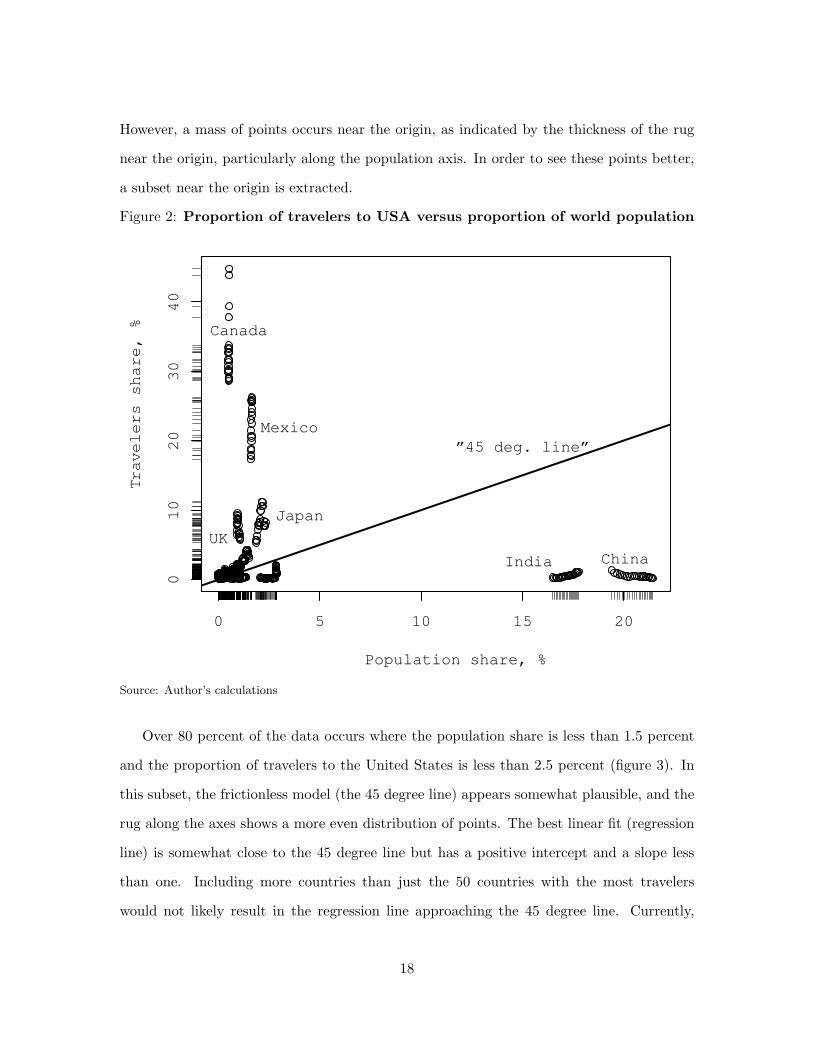
However, a mass of points occurs near the origin, as indicated by the thickness of the rug

near the origin, particularly along the population axis. In order to see these points better,

a subset near the origin is extracted.

Figure 2: Proportion of travelers to USA versus proportion of world population

0 5 10 15 20

010

20

30

40

Population share, %

Travelers share, %

ChinaIndia

Canada

Mexico

Japan

UK

”45 deg. line”

Source: Author’s calculations

Over 80 percent of the data occurs where the population share is less than 1.5 percent

and the proportion of travelers to the United States is less than 2.5 percent (figure 3). In

this subset, the frictionless model (the 45 degree line) appears somewhat plausible, and the

rug along the axes shows a more even distribution of points. The best linear fit (regression

line) is somewhat close to the 45 degree line but has a positive intercept and a slope less

than one. Including more countries than just the 50 countries with the most travelers

would not likely result in the regression line approaching the 45 degree line. Currently,

18

disproportionate numbers of points fall above the 45 degree line. Adding in the more than

150 countries and 32 percent of the world population not currently included in the data

would increase the number of points with low population shares and low shares of travelers

that fall below the 45 degree line and likely result in a regression line with an intercept

closer to origin.

Figure 3: Proportion of travelers to USA (≤ 2.5%)* versus proportion of worldpopulation (≤ 1.5%)

0.0 0.2 0.4 0.6 0.8 1.0 1.2

0.0

0.5

1.0

1.5

2.0

Population share, %

Travelers share, %

regression lineslope=0.40

”45 deg. line”

* This subset represents over 80 percent of the total data.Source: Author’s calculations

However, there are no large countries with large shares of U.S. inbound travelers. In

contrast to China and India, other countries with large populations and small shares of trav-

elers do not appear in these data. For example, Indonesia, Pakistan, Nigeria, Bangladesh,

Vietnam, Ethiopia, and Egypt (whose respective ranks in world population in 2010 were

19

4th, 6th, 7th, 8th, 13th, 14th, and 15th) are not among the top 50 countries contributing

travelers to the United States. These large omitted countries all have Muslim majorities

except Ethiopia and Vietnam. As previously discussed, religious concerns are important to

many potential travelers and appear to have largely filtered majority Muslim countries out

of the top 50 data. Turkey, the 18th most populous country, is the only majority Muslim

country included in the top 50 data. GDP is another delineating factor as the 15 wealthiest

countries in 2010 are all included in the top 50 data. South Africa, which has the largest

GDP among African countries, is the only African country in the top 50 list. Also, Singa-

pore, a small, non-majority Muslim country with high per capita income is included while

larger Indonesia (majority Muslim, low capita income) is not in the top 50 data. In sum,

adding all countries would increase the number of countries with low shares of travelers to

the United States and decrease the slope of the regression line and thus credibility of the

frictionless model.

7 Estimation

This section presents the results from estimating a demand model of inbound flows of

travelers. As discussed in the section on data exploration, GDP is used for the income

variable, but data for the price variables in equation 1 are unavailable, and travel price and

distance price are used instead. The functional form of equation 1 is specified as Cobb-

Douglas, and logarithms are taken. The frictions variables are included as demand shifters.

The resulting equation to be estimated is shown below where the variables are: flows of

inbound travelers (x), travel price (p), distance price (q), income (y), the China-U.S. MOU

(M), inclusion in the Visa Waiver Program (V), the Clark-Pugh index (C), English (E),

Spanish (S), Canada or Mexico (A), the visa refusal rate (r), and waiting times to obtain a

visa (w); where lower case letters indicate that the variable is in logarithms and indicator

variables are in upper case; where the β′s are parameters to be estimated and ε is an error

20

term; and i indexes the country dimension and t indexes the time dimension.

xi,t = β0 + βppi,t + βqqi,t + βyyi,t + βMMi,t + βV Vi,t

+βCCi + βEEi + βSSi + βAAi + βrri + βwwi + εi,t,

i = 1, ..., N, t = 1, ..., T

(2)

First, equation 2 is estimated by pooled ordinary least squares (POLS), which will serve

as a reference point for other approaches. Results are shown in table 2, and parameter

estimates for travel price, distance price, GDP, the Visa Waiver Program, the Clark-Pugh

index, English, Spanish, Canada-Mexico, and visa waiting times are statistically significant.

Although most signs are as expected, estimates for travel price and Clark-Pugh are unex-

pectedly positive. Estimates for the China MOU and visa refusal rates are not statistically

significant.25

Travelers to the United States incur varying costs and face different prices because

information and institutions affecting price vary over countries. Cultural differences also

influence which representative travelers will journey to the United States. Variables in the

model capture much of this heterogeneity, but the price variables based on indexes may not

sufficiently represent prices faced by representative travelers from different countries, and

despite the variables for cultural and policy frictions, some country-specific heterogeneity

may remain. Similarly, business cycles and other global events affect a traveler’s ability and

willingness to travel in different years. Results from the pooled model will be biased if sub-

stantial unobserved heterogeneity exists among different countries or at different times. The

Honda Lagrange multiplier test (Honda 1985) was used to test the residuals of the pooled

models for unobserved heterogeneity. The result of this test, 84.91 (with a p-value of 2.22e-

16), convincingly rejects the null hypothesis of no significant differences among countries

and time periods. Thus, there is unobserved heterogeneity that should be addressed.

25To examine the effect of using the maximum likelihood procedure to estimate the missing 2010 data ontravelers, the same POLS model was estimated using only the original data, and excluding the intercept,the average difference in the coefficient estimates was 0.0008. This suggests that the procedure to estimatethese missing data has little effect on the parameter estimates.

21

Table 2: Results: POLS, random effects, and fixed effects models

Variable POLS Random Keum Fixed effects

Intercept -0.054 -7.191∗∗∗ 4.444∗∗∗

(0.578) (1.395) (1.526)Travel price 0.062∗∗∗ -0.212∗∗∗ -0.323∗∗∗

(0.012) (0.023) (0.026)Distance price -0.453∗∗∗ -0.004 0.190∗∗

(0.045) (0.062) (0.077)GDP 0.562∗∗∗ 0.713∗∗∗ 0.756∗∗∗ 0.937∗∗∗

(0.022) (0.043) (0.042) (0.055)China MOU 0.032 0.359∗∗∗ 0.236∗∗

(0.390) (0.124) (0.119)Visa Waiver 0.479∗∗∗ 0.099∗∗∗ 0.097∗∗∗

(0.068) (0.037) (0.035)Similarity -0.058∗∗

(0.024)

Clark-Pugh 0.087∗∗∗ 0.235∗∗∗

(0.026) (0.078)English 1.067∗∗∗ 1.463∗∗∗

(0.092) (0.304)Spanish 0.512∗∗∗ 1.085∗∗∗

(0.069) (0.233)Canada-Mexico 2.587∗∗∗ 2.436∗∗∗

(0.149) (0.426)Visa refusal 0.002 0.026∗∗∗

(0.002) (0.007)Visa wait 0.003∗∗∗ 0.001

(0.001) (0.003)Distance -1.292∗∗∗

(0.157)

R2 0.729 0.344 0.262 0.320

Significance levels: ∗(p ≤ 0.1), ∗∗(p ≤ 0.05), ∗∗∗(p ≤ 0.01). Standard

errors are in parentheses. Variables below the line vary only by

country; those above vary by time and country.

Source: Author’s calculations

22

Two common approaches for taking unobserved heterogeneity into account are fixed-

effects and random-effects models. The random-effects estimator is more efficient than

the fixed-effects estimator and is considered first although it has stronger assumptions.

Both country and year effects are considered in a two-way error component model. The

disturbance term from equation 2 is written as the sum of an unobservable time-specific

effect λt, an unobservable country-specific effect µi, and the remaining idiosyncratic errors

νi,t.

εi,t = λt + µi + νi,t (3)

The results from estimating the random-effects model are shown in column 2 of table

2.26 The estimate for the travel price now has the expected negative sign and is significant,

although the estimate for distant price is no longer significant. The estimate for GDP is

larger than in the POLS model and remains significant. The estimate for the China MOU

is larger and has become statistically significant. Estimates for the Visa Waiver Program,

English, Spanish, and Mexico and Canada are statistically significant and have the expected

signs. The estimate for the Clark-Pugh index continues to have a positive sign, contrary

to expectations. Also, the estimate for the visa refusal rate is small and does not have

the expected sign. The estimate for the visa waiting time is not statistically significant at

conventional significance levels.

While on the subject of random-effects models, it is interesting to test Keum’s gravity

model for Korea with these U.S. data. The results are broadly in line with his findings.

The largest estimate (in absolute value excluding the intercept) is for the distance variable.

It is negative, and its size is consistent with his conclusion that distance is important in

gravity models of travel. The estimate for GDP is less than one and similar in size to the

random-effects estimate in column 2; both distance and GDP are statistically significant.

Relative similarity is measured as the absolute value of the log difference in per-capita

income between the United States and the country of origin of the traveler. As the difference

26Different procedures exist for estimating random-effects models, a type of feasible general linear sys-tem estimation. Results are shown for the Wallace-Hussain procedure, but the Swamy-Arora and Nerloveprocedures yielded similar results.

23

in income decreases, travel is expected to increase. Contrary to Keum’s finding, relative

similarity here has the expected negative sign and is significant at the 5 percent level.

Although the random-effects approach is more efficient than fixed effects, it relies on

the stronger assumption that the random effects are uncorrelated with the explanatory

variables. The possible endogeneity of the regressors with the individual effects can be tested

via a Hausman test. The Chi-square statistic (with 5 degrees of freedom) from the Hausman

test comparing the fixed-effects model to the random-effects model is approximately 18.5,

and on this basis the null hypothesis of no correlation between the random effects and the

explanatory variables is rejected. Therefore, consideration now moves from the random-

effects model to the fixed-effects model.

The fixed-effects estimator is more robust than random effects, and its estimates re-

main unbiased even when correlation exists between the fixed effects and the explanatory

variables. Although small fixed-effects models could be estimated with dummy variables

for the country and time effects, it is impractical when there are many individuals or time

periods. In these cases, the within transform (Q) is typically used. For the two-way model,

the within transform is Q = IN ⊗ IT − IN ⊗ JT − JN ⊗ IT + JN ⊗ JT , where I is an

identity matrix of dimension given by the subscript; J is a matrix of ones divided by its

dimension (given by the subscript), and ⊗ indicates the Kronecker product. Premultipli-

cation of both sides of the regression equation by this idempotent matrix gives the within

estimator for the regression coefficients βWI = (X′QX)−1X′Qy. The within transform

sweeps out the country effects (µi) and the time effects (λt), but unfortunately also sweeps

out any variables that do not vary with time.

Fixed-effects estimates are shown in the last column of table 2. Travel price and GDP

have the expected signs and are significant at the 1 percent level. Although still quite

inelastic, the travel price estimate is larger than in the previous models. Distance price is

positive contrary to theory. Estimates for the China MOU and the Visa Waiver Program

have the expected signs and are significant, respectively, at the 5 percent level and the 1

percent level. The estimate for the Visa Waiver Program is similar to that of the random-

24

effects model and smaller than that of the POLS model.

Major global events, including multi-country macroeconomic shocks, could affect nu-

merous countries, but individual countries will likely respond differently to these events.

While the error structure in equation 3 importantly allows time-specific effects and country

effects, all countries are restricted to a homogeneous response λt each period to any global

shock. Not taking individual countries’ responses to global events into account could result

in the idiosyncratic errors being correlated across countries at different times and compro-

mise the unbiasedness and consistency of the estimates. Methods have been developed to

test for such cross-section dependency.27 Pesaran’s CD test is based on the average of all

pairwise correlation coefficients from the model residuals and is centered on 0 under the null

hypothesis of no significant cross section dependence. Testing the residuals of the two-way

fixed-effect model yields a CD statistic of -3.082, which rejects the null hypothesis of no

significant cross-section dependence with a p-value of 0.002.28

Phillips and Sul (2003), Pesaran (2006), and others have developed models with multi-

factor error structures that allow heterogeneous responses to common shocks. Here, an

approach pioneered by Serlenga and Shin (2007) is used. The first step is to apply Pesaran’s

pooled common correlated effects (PCCE) estimator.29 In contrast to equation 3, this

model assumes the following multi-factor error structure where the γi’s are heterogeneous

country-specific responses to unobserved common time-specific effects λt’s, the µi’s are the

country-specific fixed effects as before, and the νi,t’s are the idiosyncratic errors.

εi,t = γiλt + µi + νi,t (4)

27Pesaran, Ullah, and Yamagata (2008) updated an earlier test for cross-section independence by Breuschand Pagan and also compared it to the CD test developed by Pesaran (2004).

28While the two-way fixed-effects model barely fails the CD test, the one-way (country effects only) model(not shown) fails by a large margin, with a CD statistic of about 37.3 and a p-value close to 0, which indicatesto the importance of including time-specific effects.

29Pesaran (2006) proved the consistency and asymptotic normality of several common-correlated-effectsestimators; the PCCE estimator, which assumes that different countries have the same slope coefficientsalthough the unobserved common effects vary by country, had the best small sample properties and is usedin this case.

25

Setting the pooling weights equal to1

N(the usual case), the PCCE estimator is

βPCCE =

(N∑i=1

x′iMTxi

)−1( N∑i=1

x′iMTyi

)(5)

where MT = IT −HT (H′THT )

−1H ′T and H is a matrix with a column of 1s and a column

for each common factor. The PCCE estimator is a generalization of the within estimator,

and as such, in sweeping out the unobserved heterogeneous effects, it also eliminates the

time-constant variables, as does the fixed-effects estimator.30

After obtaining the PCCE estimates in the first stage, Serlenga and Shin follow an

approach similar to Hausman-Taylor (1981) to generate estimates of the time-constant

variables in a second step. They retrieve the residuals (d) from the PCCE estimation and

use a set of instrumental variables (W) to estimate the time-constant variables (C) in a

feasible general linear system approach.31 The feasible Serlenga-Shin estimator (δSS) for

the second stage is shown below:

δSS =(C′WV −1W ′C

)−1 (C′WV −1W ′d

)(6)

where V is the estimated variance of W ′ε∗. First, an OLS version of equation 6 is run,

and the residuals from this equation (ε∗) are used to estimate V in equation 6. Subsequent

iterations are made using new estimates of (ε∗) each time to recalculate V until consecutive

estimates of (δSS) differ by less than 0.0001.32

To find factors to account for the unobserved common correlated effects, Pesaran rec-

ommends considering the cross-sectional means of the exogenous time-varying variables in

the model. Here linear time trends for each cross-section are also considered. The first

30Robust standard errors are computed for the PCCE estimates using equation 74 in Pesaran (2006),which is based on equations 51 and 52 and are an adaptation of the Newey-West procedure for computingheteroskedastic and autocorrelation consistent standard errors for panel data. In this case, the Newey-Westlag window was set to 3.

31They showed the consistency of their approach in Serlenga and Shin 2007 and showed that their estimatoroutperformed two-way fixed-effects Hausman-Taylor estimation in small samples in Serlenga and Shin (2006).

32Once the feasible GLS estimator for the coefficients has converged, the covariance matrix is(C′WV −1

FGLSW′C)−1.

26

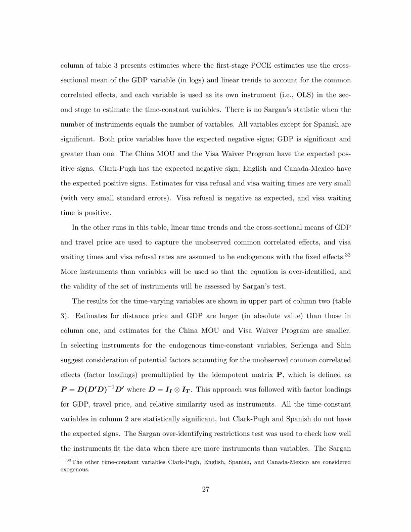
column of table 3 presents estimates where the first-stage PCCE estimates use the cross-

sectional mean of the GDP variable (in logs) and linear trends to account for the common

correlated effects, and each variable is used as its own instrument (i.e., OLS) in the sec-

ond stage to estimate the time-constant variables. There is no Sargan’s statistic when the

number of instruments equals the number of variables. All variables except for Spanish are

significant. Both price variables have the expected negative signs; GDP is significant and

greater than one. The China MOU and the Visa Waiver Program have the expected pos-

itive signs. Clark-Pugh has the expected negative sign; English and Canada-Mexico have

the expected positive signs. Estimates for visa refusal and visa waiting times are very small

(with very small standard errors). Visa refusal is negative as expected, and visa waiting

time is positive.

In the other runs in this table, linear time trends and the cross-sectional means of GDP

and travel price are used to capture the unobserved common correlated effects, and visa

waiting times and visa refusal rates are assumed to be endogenous with the fixed effects.33

More instruments than variables will be used so that the equation is over-identified, and

the validity of the set of instruments will be assessed by Sargan’s test.

The results for the time-varying variables are shown in upper part of column two (table

3). Estimates for distance price and GDP are larger (in absolute value) than those in

column one, and estimates for the China MOU and Visa Waiver Program are smaller.

In selecting instruments for the endogenous time-constant variables, Serlenga and Shin

suggest consideration of potential factors accounting for the unobserved common correlated

effects (factor loadings) premultiplied by the idempotent matrix P, which is defined as

P = D(D′D)−1D′ where D = II ⊗ IT . This approach was followed with factor loadings

for GDP, travel price, and relative similarity used as instruments. All the time-constant

variables in column 2 are statistically significant, but Clark-Pugh and Spanish do not have

the expected signs. The Sargan over-identifying restrictions test was used to check how well

the instruments fit the data when there are more instruments than variables. The Sargan

33The other time-constant variables Clark-Pugh, English, Spanish, and Canada-Mexico are consideredexogenous.

27

Table 3: Results: Pooled common correlated effects–Serlenga-Shin estimation

Variable 1 2 3 4

Travel price -0.391∗∗∗ -0.336∗∗∗ -0.336∗∗∗ -0.316∗∗∗

(0.064) (0.045) (0.045) (0.044)Distance price -0.374∗∗∗ -0.832∗∗∗ -0.832∗∗∗ -0.894∗∗∗

(0.014) (0.011) (0.011) (0.011)GDP 1.124∗∗∗ 1.534∗∗∗ 1.534∗∗∗ 1.512∗∗∗

(0.013) (0.011) (0.011) (0.011)China MOU 0.411∗∗∗ 0.232∗∗∗ 0.232∗∗∗ 0.246∗∗∗

(0.009) (0.008) (0.008) (0.008)Visa Waiver 0.083∗∗∗ 0.068∗∗ 0.068∗∗ 0.063∗∗

(0.028) (0.026) (0.026) (0.028)

Clark-Pugh -0.029∗∗∗ 0.050∗∗∗ 0.001 0.052∗∗

(0.006) (0.018) (0.019) (0.021)English 0.141∗∗∗ 0.306∗∗∗ 0.348∗∗∗ 0.423∗∗∗

(0.019) (0.055) (0.068) (0.092)Spanish 0.006 -0.498∗∗∗ 0.175∗ -0.776∗∗∗

(0.016) (0.116) (0.106) (0.219)Canada-Mexico 0.981∗∗∗ 1.507∗∗∗ 1.216∗∗∗

(0.028) (0.126) (0.098)Visa refusal -0.006∗∗∗ -0.023∗∗∗ -0.029∗∗∗ -0.025∗∗∗

(0.001) (0.003) (0.003) (0.004)Visa wait 0.002∗∗∗ 0.060∗∗∗ 0.025∗∗ 0.077∗∗∗

(0) (0.011) (0.011) (0.019)

Sargan test 0.18 7.55 0.34[0.671] [0.006] [0.560]

Significance levels: ∗(p ≤ 0.1), ∗∗(p ≤ 0.05), ∗∗∗(p ≤ 0.01). Standard

errors in parentheses. P-values for the Chi-square Sargan test with 1 degree

of freedom are shown in brackets. Variables below the line vary only by

country; those above vary by time and country.

Source: Author’s calculations.

28

test for column two is small, and the null hypothesis that these instruments are valid is not

rejected.34 From a statistical point of view, the results in column two could be considered

the best in the study.

Traditional Hausman-Taylor estimation uses the exogenous time-varying variables pre-

multiplied by P as instruments for the endogenous time-constant variables. Here GDP,

travel price, and the Visa Waiver Program are considered exogenous, and the results are

presented in column three. The main difference from the instruments used in column two

is that the estimate for Clark-Pugh is no longer significant. However, the Sargan test

for column three is somewhat large, and one would reject the null hypothesis that these

instruments are valid at usual levels of significance.

Because travelers from Canada and Mexico dominate the number of inbound travelers,

a check was made on the effect of removing those two countries from the data. A run was

made without Canada and Mexico using the same setup as column two (except, of course, an

indicator for Canada and Mexico could not be included). The results, presented in column

4, only changed by small amounts, particularly for the time-varying variables, although the

effect of distance price is somewhat greater. The most striking changes are that without the

inclusion of Mexico, the estimate for Spanish becomes more negative, and the estimate for

English becomes more positive. Sargan’s test is small, and these instruments, as in column

two, are considered valid.

8 Conclusion

The empirical results support the basic demand model and show that many of the travel

frictions, but not all, are key determinants of U.S. inbound travel. Estimation methods that

allowed for the possibility of common correlated effects produced the most reasonable and

statistically valid results.

Income is the most significant determinant of inbound travel to the United States.

34In this case, as in the other columns of table 3, the number of instruments exceeds the number ofendogenous variables by one, and the Sargan test has a chi-square distribution with one degree of freedom.

29

Income as represented by GDP was highly significant with p-values less than 0.01 in every

run; additionally, wealthier countries appeared in the top 50 data with high frequency, as

detailed in the section on the frictionless model. The income variable was greater than

one in all runs that permitted country-specific responses to global shocks. The estimates

in this log-log format imply that the income elasticity exceeds one; thus travel to United

States increases more than proportionally as income rises (and also declines more than

proportionally with falls in income).

Travel price, which represents U.S. prices relative to prices in the originating country, is

an important determinant of inbound U.S. travel. In every run with country-specific effects

in response to global events, travel price had the expected negative sign and was highly

significant with p-values less than 0.01. In these runs, estimates were inelastic, in the range

of -0.3 to -0.4, which indicates that numbers of travelers respond less than proportionally

to changes in travel prices.

Distance price similarly has a major influence on numbers of inbound travel in most

runs. It is negative and significant with p-values less than 0.01 in the runs with the multi-

factor errors, but varies more than travel price. These latter estimates are inelastic as

well, although not as much so as travel price. Thus, travelers respond somewhat to shorter

distances and improving transportation prices.

The estimates representing income and prices, especially those in table 3, affirm the

standard demand model. The importance of accounting for the common correlated effects

can be seen by contrasting these results with those in table 2 where one of the price variables

had an unexpected sign or was not statistically significant in several instances. Thus,

economic factors collectively exert a strong influence on numbers of inbound travelers.

The Visa Waiver Program contributed to additional visits to the United States from

countries participating in the program; estimates with the common correlated effects show

that travelers from countries participating in the program were 7 to 9 percent more likely to

visit the United States than travelers from countries not in the program.35 These estimates

35The marginal effect for a dummy variable with a coefficient c from a regression with a logarithmicresponse variable is ec − 1, Halvorsen and Palmquist (1980) and Giles (2011).

30

were significant with p-values less than 0.05. The fairly small number of countries in the

program moderates the magnitude of this effect. For example, some large countries (e.g.,

China, India, Brazil, Russia, and Korea) in the top 50 data do not participate in the

program, and slightly less than half of the countries in the program appear in the top

50 data. As discussed in the section on travel frictions, many recent inductees into the

program, except for Taiwan, are relatively small Eastern European countries.

Parameter estimates for the China MOU had the expected sign, were statically signif-

icant with p-values less than 0.01, and imply that the MOU has led to increases of ap-

proximately 26 percent in numbers of U.S. inbound travelers for the runs with the common

correlated effects. It is somewhat incredulous that a program benefiting a single country

(neither of which is Canada or Mexico) would have this large of an effect, at least in the

long run. Although the variables accounting for unobserved heterogeneity include country-

specific linear time trends, numbers of travelers from China grew much more than trend

during 2008 to 2010, a time when numbers of visitors from many other countries were stag-

nant or declining. Signing the MOU could have released pent-up demand as the United

States was one of the last countries with which China negotiated a travel MOU. Three years

is short time on which to make an inference, and a longer series of data would likely result

in smaller increases in numbers of Chinese visitors. The available data, however, show that

the China MOU has a major positive influence on numbers of inbound U.S. travelers.

Parameter estimates for the visa refusal rate were significant with p-values less than 0.01

for the runs with the common correlated effects. However, the effects were very small; a 1

percent increase in the visa refusal rate is estimated to decrease numbers of inbound travelers

by 0.02 percent. Visa refusal rates do not thus appear to be an important determinant of

inbound U.S. travel.

Parameter estimates for waiting times to obtain a visa tended to be positive, possibly

indicating that large numbers of applicants are straining consulate resources in countries

where travel to the United States is popular. A one percent increase in visa waiting times

is estimated to increase numbers of inbound travelers by approximately 0.06 percent. Al-

31

though estimates for visa waiting times had p-values less than 0.01 in the runs with the

common correlated effects, their low magnitudes show that visa waiting times are not a

major determinant of inbound travel.

Sharing a border with the United States is a significant determinant of inbound U.S.

travel, as travelers were generally two to three times more likely to be from Canada or

Mexico than from any other country. The effects from sharing a border were large and

significant with p-values less than 0.01 for every run in which they were included.

Being from an English-speaking country is a significant determinant of inbound U.S.

travel; estimates were consistently statistically significant with p-values less than 0.01. In-

dications (based on table 3, column 2) are that an inbound traveler is about 36 percent more

likely to hail from an English-speaking country than from a non-English-speaking one.

Parameter estimates for Spanish in the runs with common correlated effects were either

negative, indicating that travelers are less likely to be from Spanish-speaking countries than

from other countries, or statistically insignificant. In the section on data exploration, it was

noted that majority Spanish-speaking countries constitute 28 percent of the countries in

the top 50 data, which was greater than the percentage of English-speaking countries. One

explanation is that Spanish-speaking countries are likely to be among the group of countries

most likely to visit the United States, but are less likely to be a source of U.S. inbound

travelers than other countries in that top group.

The only run in which the Clark-Pugh index had the expected sign and was statistically

significant was the common correlated-effects run where each variable was its own instru-

ment. In the other instances, it was not significant or was positive, which indicates that

travelers with cultures less like the United States are more likely to visit the United States.

Although the Clark-Pugh index is a parsimonious indicator of cultural factors, it could be

that the categories, which group the United States and South Africa in the same cluster,

Belgium and Argentina in the same cluster, and many different countries in a rest-of-the-

world cluster, are too broad to be meaningful in this context. The Clark-Pugh index thus

does not appear to be an important determinant of inbound U.S. travel.

32

References

[1] Anderson, James E. September 2011. “The Gravity Model.” Annual Review of Eco-

nomics 3: 133-160.

[2] Arita, Shawn, Sumner La Croix, and James Mak. June 2012. “How Big? The Impact

of Approved Destination Status on Mainland Chinese Travel Abroad,” Univ. of Hawaii,

Economic Research Organization Working Paper 2012-4.

[3] Baltagi, Badi H. 2008. Econometric Analysis of Panel Data, 4th edition. Wiley, Chich-

ester, West Sussex, UK.

[4] Belenkiy, Maksim. March 2012. “International Leisure Travelers to the United States:

Why Do Visitors Who Need a Visa Stay Longer?” U.S. Dept. of Commerce, Working

Paper.

[5] Bergstrand, Jeffrey H. and Peter Egger. 2011. “Gravity Equations and Economic Fric-

tions in the World Economy.” In Palgrave Handbook of International Trade, edited by

Daniel Bernhofen, Rodney Ralvey, David Greenway and Udo Krieckemeier.

[6] Clark, Timothy and Derek S. Pugh. June 2001. “Foreign Country Priorities in the

Internationalization Process: A Measure and an Exploratory Test on British Firms,”

International Business Review 10, iss. 3: 285–303.

[7] Divisekera, Sarath. 2003. “A Model of Demand for International Tourism.” Annals of

Tourism Research 30, no. 1: 31–49.

[8] Eita, Joel Hinaunye, Andre C. Jordaan, and Yolanda Jordaan. February 2011. “An

Econometric Analysis of the Determinants Impacting on Businesses in the Tourism

Industry.” African Journal of Business Management 5, no. 3: 666–675.

[9] Giles, David E. January 2011. “Interpreting Dummy Variables in Semi-logarithmic Re-

gression Models: Exact Distributional Results.” Univ. of Victoria, Econometrics Work-

ing Paper EWP1101.

33

[10] Halvorsen, Robert and Raymond Palmquist. June 1980. “The Interpretation of Dummy

Variables in Semilogarithmic Equations.” The American Economic Review 70, no. 3:

474-475.

[11] Hausman, Jerry A. and William E. Taylor. 1981. “Panel Data and Unobservable Indi-

vidual Effects.” Econometrica 49, no. 6: 1377–1398.

[12] Honda, Y. 1985. “Testing the Error Components Model with Non-normal Distur-

bances.” Review of Economic Studies 52: 681–690.

[13] Keum, Kiyong . 2010. “Tourism Flows and Trade Theory: A Panel Data Analysis with

the Gravity Model.” Annals of Regional Science 44: 541-557.

[14] Lim, Christine. 1997. “Review of International Tourism Demand Models.” Annals of

Tourism Research 24: 835–849.

[15] Lim, Christine and Michael McAleer. 2001. “Modelling the Determinants of Interna-

tional Tourism Demand to Australia.” Institute of Social and Economic Research, Osaka

Univ., Working Paper.

[16] Linder, Staffan. 1961. An Essay on Trade and Transformation. Almqvist & Wiksell,

Stockholm.

[17] Long, Wesley H. 1970. “The Economics of Air Travel Gravity Models.” Journal of

Regional Science 10, no. 5: 353-363.

[18] Mak, James. 2004. Tourism and the Economy: Understanding the Economics of

Tourism. Univ. of Hawaii Press, Honolulu.

[19] Naude, Willem A. and Andrea Saayman. 2005. “Determinants of Tourist Arrivals in

Africa: A Panel Data Regression Analysis.” Tourism Economics 11, no. 3: 365–391.

[20] Neumayer, Eric. 2010. “Visa Restrictions and Bilateral Travel.” The Professional Ge-

ographer 62, no. 2: 171–181.

34

[21] Ng, Siew Imm, Julie Anne Lee, and Geoffrey N. Soutar. 2007. “Tourists Intention to

Visit a Country: The Impact of Cultural Distance.” Tourism Management 28, iss. 6:

1497–1506.

[22] Pesaran, M. Hashem, Aman Ullah, and Takashi Yamagata. 2008. “A Bias-adjusted LM

Test of Error Cross-section Independence.” Econometrics Journal 11, iss. 1: 105–127.

[23] Pesaran, M. Hashem. 2006. “Estimation and Inference in Large Heterogeneous Panels

with a Multifactor Error Structure.” Econometrica 74, no. 4: 967–1012.

[24] Pesaran, M. Hashem. 2004. “General Diagnostic Tests for Cross Section Dependence

in Panels.” CESIFO Working Paper No. 1229.

[25] Pew Hispanic Center. April 22, 2010. “Hispanics of Mexican Origin in the United

States, 2008.” Fact Sheet. http://pewhispanic.org/files/factsheets/59.pdf

[26] Phillips, Peter C.B. and Donggyu Sul. 2003. “Dynamic Panel Estimation and Homo-

geneity Testing under Cross Section Dependence.” Econometrics Journal 6, 217–259.

[27] Serlenga, Laura and Yongcheol Shin. 2007. “Gravity Models of Intra-EU Trade: Appli-

cations of the CCEP-HT Estimation in Heterogeneous Panels with Unobserved Common

Time-Specific Factors.” Journal of Applied Econometrics 22: 361-381.

[28] Serlenga, Laura and Yongcheol Shin. 2006. “Monte Carlo Studies on Finite Sample

Performance of the CCEP-HT Estimator in Panels with Heterogeneous Unobserved

Common Factors.” Working Paper, University of Leeds.

[29] Su, Yu-Sung, Andrew Gelman, Jennifer Hill, and Masanao Yajima. 2011. “Multiple

Imputation with Diagnostics in R: Opening Windows into the Black Box.” Journal of

Statistical Software 45, iss. 2: 1–31.

[30] Vietze, Christoph. 2008. “Cultural Effects on Inbound Tourism into the USA: A Gravity

Approach.” Jena Economic Research Papers 2008-037.

35

[31] Vogel, Harold L. 2001. Travel Industry Economics: A Guide for Financial Analysis.

Cambridge University Press.

[32] World Trade Organization 2011. International Trade Statistics 2011. http://www.wto.

org/english/res_e/statis_e/its2011_e/its11_toc_e.htm. downloaded, December

15, 2011.

[33] World Travel and Tourism Council. 2012. “Travel & Tourism Economic Impact 2012.”

36