designing and implementing a regional urban modeling...

Computers, Environment and Urban Systems xxx (2009) xxx–xxx

ARTICLE IN PRESS

Contents lists available at ScienceDirect

Computers, Environment and Urban Systems

journal homepage: www.elsevier .com/locate /compenvurbsys

Designing and implementing a regional urban modeling system usingthe SLEUTH cellular urban model

Claire A. Jantz a,*, Scott J. Goetz b,1, David Donato c,2, Peter Claggett d,3

a Geography-Earth Science Department, Shippensburg University, 1871 Old Main Dr., Shippensburg, PA 17257, USAb The Woods Hole Research Center, 149 Woods Hole Road, Falmouth, MA 02540, USAc US Geological Survey, 12201 Sunrise Valley Drive [MS 521], Reston, VA 20192, USAd US Geological Survey, Chesapeake Bay Program Office, 410 Severn Ave., Suite 109, Annapolis, MD 21403, USA

a r t i c l e i n f o

Article history:Received 21 February 2009Received in revised form 19 August 2009Accepted 19 August 2009Available online xxxx

Keywords:Urban modelingUrban simulationCellular automataSLEUTHChesapeake Bay

0198-9715/$ - see front matter � 2009 Elsevier Ltd. Adoi:10.1016/j.compenvurbsys.2009.08.003

* Corresponding author. Tel.: +1 717 477 1399; faxE-mail addresses: [email protected] (C.A. Jantz), s

[email protected] (D. Donato), PClagget@chesapeake1 Tel.: +1 508 540 9900.2 Tel.: +1 703 648 5772.3 Tel.: +1 410 267 5771.

Please cite this article in press as: Jantz, C. A., etComputers, Environment and Urban Systems (200

a b s t r a c t

This paper presents a fine-scale (30 meter resolution) regional land cover modeling system, based on theSLEUTH cellular automata model, that was developed for a 257000 km2 area comprising the ChesapeakeBay drainage basin in the eastern United States. As part of this effort, we developed a new version of theSLEUTH model (SLEUTH-3r), which introduces new functionality and fit metrics that substantiallyincrease the performance and applicability of the model. In addition, we developed methods that expandthe capability of SLEUTH to incorporate economic, cultural and policy information, opening up new ave-nues for the integration of SLEUTH with other land-change models. SLEUTH-3r is also more computation-ally efficient (by a factor of 5) and uses less memory (reduced 65%) than the original software. With thenew version of SLEUTH, we were able to achieve high accuracies at both the aggregate level of 15 sub-regional modeling units and at finer scales. We present forecasts to 2030 of urban development undera current trends scenario across the entire Chesapeake Bay drainage basin, and three alternative scenariosfor a sub-region within the Chesapeake Bay watershed to illustrate the new ability of SLEUTH-3r to gen-erate forecasts across a broad range of conditions.

� 2009 Elsevier Ltd. All rights reserved.

1. Introduction

The objective of this paper is to describe a regional urban landcover modeling system that was developed for the ChesapeakeBay watershed, which is located in the eastern United States(Fig. 1). We developed a fine-scale (30 meter � 30 meter or 0.09hectare cell size) regional modeling system, based on the SLEUTHurban land-cover change model (Clarke, Hoppen, & Gaydos,1997; US Geological Survey, 2007) and applied it to forecastgrowth up to the year 2030 for the Chesapeake Bay watershed(CBW) and adjacent counties, an area covering 257,000 km2.

SLEUTH is one of a class of models known as cellular automata(CA), where the land surface is conceptually divided into cells usinga regular grid. SLEUTH then associates with each cell an automa-ton, an entity that independently executes its own state-transitionrules, taking into account the states of the automata associatedwith nearby cells. Given its success with regional scale urban sim-

ll rights reserved.

: +1 717 477 [email protected] (S.J. Goetz),bay.net (P. Claggett).

al. Designing and implementing9), doi:10.1016/j.compenvurbs

ulation, its ability to incorporate different levels of protection fordifferent areas, the relative ease of computation and implementa-tion, and the fact that it is public domain software, we adopted theSLEUTH model (Clarke et al., 1997; Clarke & Gaydos, 1998) to formthe basis for this work. SLEUTH incorporates spatial data through alink with geographic information systems (GIS) and, like many re-cently developed CAs (e.g. Van Vliet, White, & Dragicevic, 2009), re-laxes many of the assumptions of classic CA theory, such ashomogeneity of space, uniformity of neighborhood interactions,and universal transition functions, to more realistically simulatereal urban systems. Because they are interactive, modified CA mod-els like SLEUTH are attractive in applied settings as planning tools(Batty, 1997). Potential outcomes can be visualized and quantified,the models can be closely linked with GIS, and raster based spatialdata derived from remote sensing platforms can be easily incorpo-rated into the model.

The utility of CA models for simulating complex systems,including urban systems, has been well documented (Couclelis,1997; O’Sullivan & Torrens, 2000; Silva & Clarke, 2005; Torrens,2006; Torrens & O’Sullivan, 2001; Van Vliet et al., 2009). For regio-nal scale modeling, CA models have proven to be effective plat-forms for simulating dynamic spatial interactions amongbiophysical and socio-economic variables associated with land-cover change (White & Engelen, 1997). For example, Li and Liu

a regional urban modeling system using the SLEUTH cellular urban model.ys.2009.08.003

http://dx.doi.org/10.1016/j.compenvurbsys.2009.08.003

mailto:[email protected]




http://www.sciencedirect.com/science/journal/01989715

http://www.elsevier.com/locate/compenvurbsys


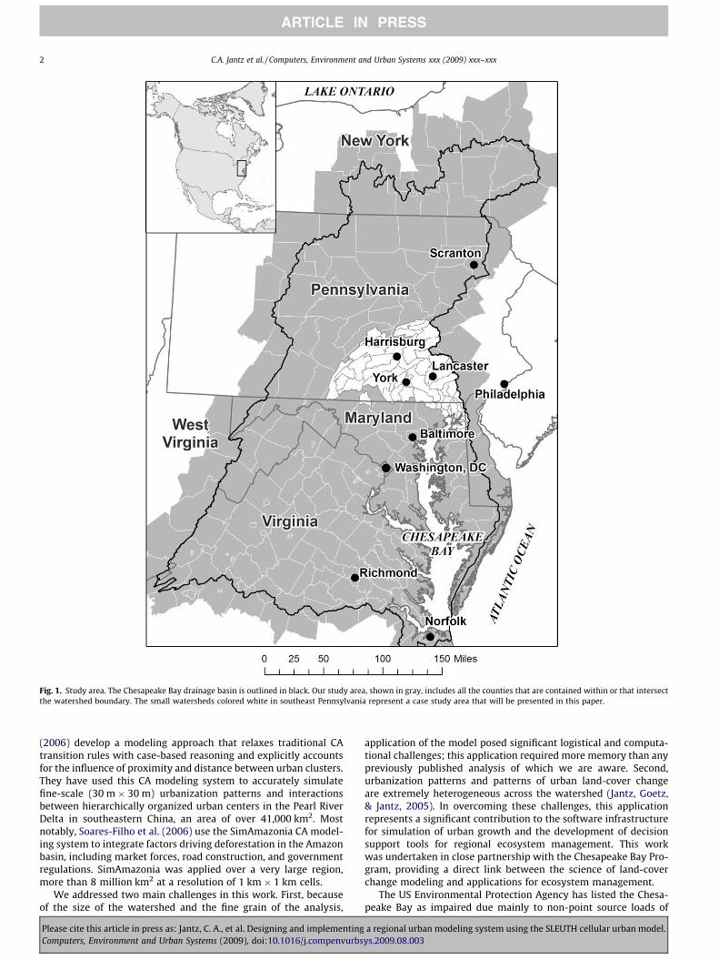
Fig. 1. Study area. The Chesapeake Bay drainage basin is outlined in black. Our study area, shown in gray, includes all the counties that are contained within or that intersectthe watershed boundary. The small watersheds colored white in southeast Pennsylvania represent a case study area that will be presented in this paper.

2 C.A. Jantz et al. / Computers, Environment and Urban Systems xxx (2009) xxx–xxx

ARTICLE IN PRESS

(2006) develop a modeling approach that relaxes traditional CAtransition rules with case-based reasoning and explicitly accountsfor the influence of proximity and distance between urban clusters.They have used this CA modeling system to accurately simulatefine-scale (30 m � 30 m) urbanization patterns and interactionsbetween hierarchically organized urban centers in the Pearl RiverDelta in southeastern China, an area of over 41,000 km2. Mostnotably, Soares-Filho et al. (2006) use the SimAmazonia CA model-ing system to integrate factors driving deforestation in the Amazonbasin, including market forces, road construction, and governmentregulations. SimAmazonia was applied over a very large region,more than 8 million km2 at a resolution of 1 km � 1 km cells.

We addressed two main challenges in this work. First, becauseof the size of the watershed and the fine grain of the analysis,

Please cite this article in press as: Jantz, C. A., et al. Designing and implementingComputers, Environment and Urban Systems (2009), doi:10.1016/j.compenvurbs

application of the model posed significant logistical and computa-tional challenges; this application required more memory than anypreviously published analysis of which we are aware. Second,urbanization patterns and patterns of urban land-cover changeare extremely heterogeneous across the watershed (Jantz, Goetz,& Jantz, 2005). In overcoming these challenges, this applicationrepresents a significant contribution to the software infrastructurefor simulation of urban growth and the development of decisionsupport tools for regional ecosystem management. This workwas undertaken in close partnership with the Chesapeake Bay Pro-gram, providing a direct link between the science of land-coverchange modeling and applications for ecosystem management.

The US Environmental Protection Agency has listed the Chesa-peake Bay as impaired due mainly to non-point source loads of



C.A. Jantz et al. / Computers, Environment and Urban Systems xxx (2009) xxx–xxx 3

ARTICLE IN PRESS

nutrients and sediment. The Chesapeake Bay Program (CBP), a fed-eral and state agency partnership established to restore the healthof the Chesapeake Bay, has agreed to over one hundred differentrestoration objectives in the areas of living resources, habitat,water quality, stewardship and sound land use (Chesapeake BayProgram, 2000). Future land use forecasts will inform many ofthese objectives. Knowing the probability of land conversion fromagriculture, wetland or forest (resource lands) to residential, com-mercial, or industrial use (built) will guide the development ofpractical alternatives and contingency plans related to Bay trendsand indicators (Jantz & Goetz, 2007).

The objective was to create an adaptive modeling system capa-ble of producing dynamic and fine-scale forecasts of urban land-change through the year 2030 within the CBW. In order to achievethis objective, these four problems had to be solved:

1. How to modify and adapt the SLEUTH model. Several mod-ifications were made to the SLEUTH model and calibrationmethodology to address scale sensitivity and the inabilityof SLEUTH to consider factors that attract and resist devel-opment. Also, SLEUTH’s performance was enhanced by aset of code modifications that substantially reduced themodel’s memory requirements and increased processingspeed.

2. How to subdivide the Chesapeake Bay watershed. Becauseof the heterogeneity of urban patterns and urban land-coverchange patterns we divided the Chesapeake Bay into 15sub-regions, ranging from roughly 7,000 km2 to 23,000km2 in size, within which urbanization patterns are rela-tively homogeneous. These subdivisions comprised the spa-tial framework of our regional modeling system.

3. How best to calibrate our revised version of the SLEUTHmodel. We calibrated SLEUTH separately for each of the 15sub-regions.

4. How to select alternative futures for the CBW. A Bay-wideforecast of future urbanization in 2030 under a ‘‘currenttrends” scenario was completed. We also developed twoadditional policy and growth scenarios to assess the utilityof this modeling approach. We illustrate the use of thesealternative scenarios using results for a generally represen-tative sub-region, southeast Pennsylvania (Fig. 1).

2. Methods

2.1. Overview of the SLEUTH model

SLEUTH simulates urban dynamics through the application offour growth rules: spontaneous new growth, which simulates therandom urbanization of land; new spreading center growth, orthe establishment of new urban centers; edge growth; and roadinfluenced growth. Each type of growth is controlled by an area-wide coefficient (diffusion, breed, spread, road growth) that canrange in value from 0 to 100, reflecting the relative contributionof a particular growth type to urban dynamics within a study area.The resistance of development to slope is also controlled by a cal-ibrated parameter, the slope coefficient, which ranges from 0 to100 (0 indicating low slope resistance, 100 indicating high sloperesistance). The user can specify additional resistance rules in anexcluded layer, which indicates areas that are partially or com-pletely excluded from development.

Implementation of the model occurs in two general phases: cal-ibration, where historic growth patterns are simulated; and predic-tion, where historic patterns of growth are projected into thefuture. For calibration, the original SLEUTH model requires inputsof historic urban extent for at least four time periods, a historic


transportation network for at least two time periods, slope, andan excluded layer.

2.2. Modifications to the SLEUTH model

In our previous work with the SLEUTH model, we identified sev-eral limitations. First, when fine resolution data are used, SLEUTHis not always able to generate an appropriate level of dispersedgrowth because of SLEUTH’s bias towards edge growth (Jantz &Goetz, 2005).

Second, most of the fit statistics that have commonly been usedto calibrate the model are least squares regression scores (r2) mea-suring the relationship between a particular simulation of urbani-zation and actual (historic) observed urbanization. Thus thehistoric input data sets used in calibration must cover at least fourpoints in time: one to initialize the model and three additional con-trol points to calculate the regression equation. In addition, use ofthe r2 statistic alone can result in an under- or over-fitting of themodel. Without additional information, such as the y-intercept ofthe linear regression equation, a user may identify a simulationthat appears to perform well but is actually over- or under-esti-mating growth rates or patterns.

Third, SLEUTH utilizes computer memory inefficiently. For lar-ger data sets, Unix or Linux based parallel computing is typicallyused to calibrate the model, but the Chesapeake Bay data set ex-ceeded the memory capacity of our available computing resources(memory requirements ranged from 1.4 GB to more than 5 GB),even when divided into sub-regions.

Finally, SLEUTH usually only incorporates factors that constraindevelopment (Jantz, Goetz, & Shelley, 2004). Providing an ability toidentify areas where growth is more likely to occur will increase theutility of the model, both in terms of improving SLEUTH’s ability tosimulate historic patterns and in developing scenarios of futuredevelopment.

The first three points presented above were addressed throughdirect modification of SLEUTH’s source code (written in the C pro-gramming language), resulting in a new version of SLEUTH,SLEUTH 3.0beta_p01 Version R (referred to here as SLEUTH-3r).The fourth point (attracting growth) was addressed methodologi-cally during calibration, as discussed below in Section 2.3.

The source code changes discussed in this section thus consistof three primary modifications to: (i) address scale sensitivity,(ii) calculate new fit metrics, and (iii) decrease SLEUTH’s memoryrequirements and optimize processing speed. A general discussionof these changes is presented here. Technical descriptions areavailable with the model’s source code, which can be downloadedfrom the USGS Eastern Geographic Science Center’s (EGSC) High-Performance Computing Cluster (HPCC) website (http://egscbeo-wulf.er.usgs.gov/geninfo/downloads/). We emphasize thatSLEUTH-3r represents added functionality to SLEUTH; the originalfunctions of SLEUTH are completely retained, as are the originaltheoretical underpinnings.

2.2.1. Modifications to address scale sensitivitySLEUTH’s inability to capture dispersed settlements patterns

and its tendency to allow edge growth to dominate the systemare both related to the number of pixels that the model selectsfor potential new spontaneous development in any time step. Inthe original code, the number of spontaneous urbanization at-tempts (the dispersion value) depends on the calibrated value forthe diffusion coefficient, a constant multiplier, and the number ofpixels in the image diagonal, a convention embedded in the origi-nal source code (US Geological Survey, 2007):

DV ¼ DC � DM �ffiffiffiffiffiffiffiffiffiffiffiffiffiffiffiffiR2 þ C2

q


http://egscbeowulf.er.usgs.gov/geninfo/downloads/

http://egscbeowulf.er.usgs.gov/geninfo/downloads/



ARTICLE IN PRESS

where DV is the dispersion value, DC is the diffusion coefficient, DM

is the diffusion coefficient multiplier (a constant equal to 0.005 inthe original version of SLEUTH), R is the number of rows and C isthe number of columns.

In SLEUTH-3r, DM is no longer a constant, allowing the user tochange this multiplier value interactively. When the multiplier isincreased or decreased, the number of urbanization attempts fordiffusion growth changes accordingly. DM must be set prior tobeginning calibration. To discover an appropriate multiplier value,SLEUTH-3r’s growth coefficients were set to produce the maximumlevel of spontaneous new growth (i.e. diffusion was set to 100 andall other growth coefficients set to 0) (Jantz & Goetz, 2005). Then,several simulations are performed with SLEUTH-3r in calibrationmode to test different values for DM, simulating growth over thelength of the historic urban time series. When DM is set such thatSLEUTH-3r is able to capture, or even over-estimate, the numberof urban clusters (as measured by the cluster fractional differencemetric, a new pattern metric discussed below), normal calibrationprocedures can be initiated (see Section 2.3) to identify the bestvalues for SLEUTH-3r’s growth coefficients.

2.2.2. New calibration statisticsIn addition to the ability to interactively set the diffusion coef-

ficient multiplier, SLEUTH-3r now also creates new tabular filesthat include difference and ratio metrics that directly comparethe modeled variable (e.g. number of urban clusters) with the ob-served variable for all control dates. Specifically, SLEUTH-3r calcu-lates (i) the algebraic difference between the observed value andmodeled value, (ii) the ratio of the modeled value to the observedvalue, and (iii) the fractional change in the modeled value relativeto the observed value. It does this for most of the original fit statis-tics, for each run, and for each control year.

When at least four control points are available, these new fitmetrics can be used in conjunction with the r2 values to enhancethe calibration procedure. When fewer than three control pointsare available, the new metrics can be the principal means for cali-brating SLEUTH-3r. Table 1 presents a list of the new fit metricsavailable in SLEUTH-3r.

2.2.3. Decreasing memory requirements and improving processingspeed

The final set of modifications made to SLEUTH’s source codeaddressed the model’s memory requirements and computationalspeed. SLEUTH requires space in RAM for numerous internal cellarrays, each with the same dimensions as the modeling unit; ourapplications required about 18 of these internal cell arrays, sothe largest modeling unit in our study area would require spacein RAM for more than 1.4 billion cells. Because available versionsof SLEUTH required 4 bytes of RAM for each cell, our largest sub-

Table 1New fit metrics available in SLEUTH-3r. For each of the metrics described below, SLEUTH-between the observed value and modeled value (diff), (ii) the ratio of the modeled value toto the observed value (fract). Measurements derived from the modeled data are averaged

Fit statistic Definition

Pixels (pix) Modeled urban pixels compared to actual urban pixels for eaEdges (edges) Modeled urban edge pixels compared to actual urban edgeClusters (clusters) Modeled number of urban clusters compared to actual urban

In cell space, clusters can consist of a single pixel or multipleCluster size

(mn_cl_sz)Modeled average cluster size compared to actual average u

Slope (avg_slope) The average slope for modeled urban pixels compared to ac% Urban (pct_urba) The percent of available pixels urbanized during simulationX-mean (xmean) Average x-axis values for modeled urban pixels compared tY-mean (ymean) Average y-axis values for modeled urban pixels compared tRadius (radius) Average radius of the circle that encloses the simulated urb


region would require more than 5.6 Gigabytes of RAM, whichexceeded the 2.0 Gigabyte maximum program size under the 32-bit computer operating systems used by the vast majority of users.

Calibrating with the existing versions of SLEUTH was a compu-tationally intensive process for which the required computer pro-cessing time was roughly proportional to the size of the modelingunit. Our relatively large sub-regional modeling units would thusrequire extensive and lengthy calibration computations.

A review of the SLEUTH source code revealed that only one byteof RAM per cell was actually required in any of the internal cell ar-rays (grids) because the largest number required to be stored forany one cell was 255 or less. Since all integers between 0 and255 can be represented by a single 8-bit byte of computer storage(using the C-language ‘‘unsigned char” data type), in SLEUTH-3r wecould use a single byte per cell in the SLEUTH internal arrays in-stead of the four-byte value which had been allocated in standardSLEUTH. We incorporated this change into SLEUTH-3r and success-fully tested it to insure that the change did not introduce any spu-rious artifacts. With this change in place, we were able to useSLEUTH-3r with our relatively large modeling units.

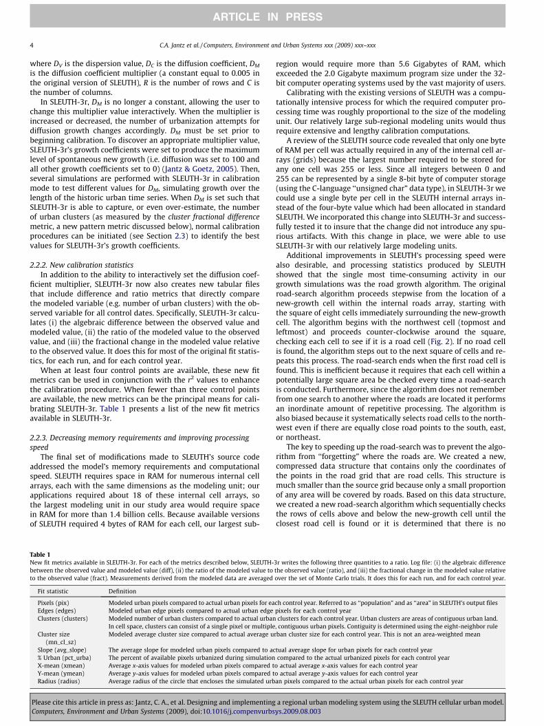
Additional improvements in SLEUTH’s processing speed werealso desirable, and processing statistics produced by SLEUTHshowed that the single most time-consuming activity in ourgrowth simulations was the road growth algorithm. The originalroad-search algorithm proceeds stepwise from the location of anew-growth cell within the internal roads array, starting withthe square of eight cells immediately surrounding the new-growthcell. The algorithm begins with the northwest cell (topmost andleftmost) and proceeds counter-clockwise around the square,checking each cell to see if it is a road cell (Fig. 2). If no road cellis found, the algorithm steps out to the next square of cells and re-peats this process. The road-search ends when the first road cell isfound. This is inefficient because it requires that each cell within apotentially large square area be checked every time a road-searchis conducted. Furthermore, since the algorithm does not rememberfrom one search to another where the roads are located it performsan inordinate amount of repetitive processing. The algorithm isalso biased because it systematically selects road cells to the north-west even if there are equally close road points to the south, east,or northeast.

The key to speeding up the road-search was to prevent the algo-rithm from ‘‘forgetting” where the roads are. We created a new,compressed data structure that contains only the coordinates ofthe points in the road grid that are road cells. This structure ismuch smaller than the source grid because only a small proportionof any area will be covered by roads. Based on this data structure,we created a new road-search algorithm which sequentially checksthe rows of cells above and below the new-growth cell until theclosest road cell is found or it is determined that there is no

3r writes the following three quantities to a ratio. Log file: (i) the algebraic differencethe observed value (ratio), and (iii) the fractional change in the modeled value relativeover the set of Monte Carlo trials. It does this for each run, and for each control year.

ch control year. Referred to as ‘‘population” and as ‘‘area” in SLEUTH’s output filespixels for each control yearclusters for each control year. Urban clusters are areas of contiguous urban land.

, contiguous urban pixels. Contiguity is determined using the eight-neighbor rulerban cluster size for each control year. This is not an area-weighted mean

tual average slope for urban pixels for each control yearcompared to the actual urbanized pixels for each control year

o actual average x-axis values for each control yearo actual average y-axis values for each control yearan pixels compared to the actual urban pixels for each control year



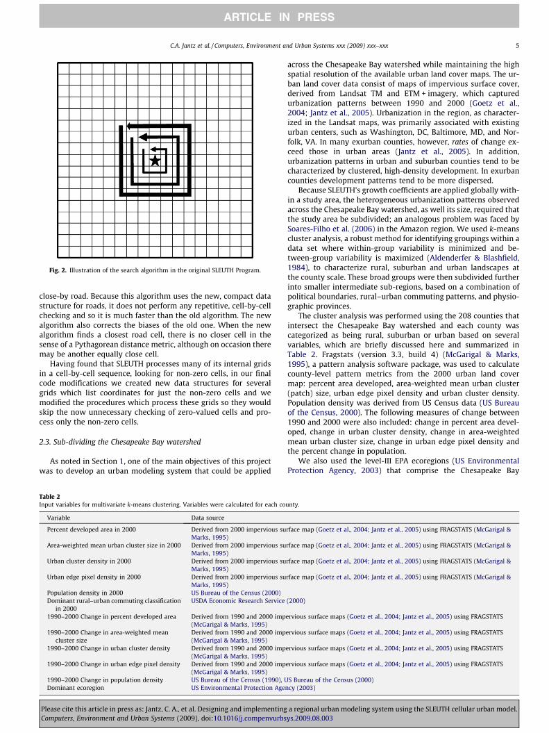
Fig. 2. Illustration of the search algorithm in the original SLEUTH Program.


ARTICLE IN PRESS

close-by road. Because this algorithm uses the new, compact datastructure for roads, it does not perform any repetitive, cell-by-cellchecking and so it is much faster than the old algorithm. The newalgorithm also corrects the biases of the old one. When the newalgorithm finds a closest road cell, there is no closer cell in thesense of a Pythagorean distance metric, although on occasion theremay be another equally close cell.

Having found that SLEUTH processes many of its internal gridsin a cell-by-cell sequence, looking for non-zero cells, in our finalcode modifications we created new data structures for severalgrids which list coordinates for just the non-zero cells and wemodified the procedures which process these grids so they wouldskip the now unnecessary checking of zero-valued cells and pro-cess only the non-zero cells.

2.3. Sub-dividing the Chesapeake Bay watershed

As noted in Section 1, one of the main objectives of this projectwas to develop an urban modeling system that could be applied

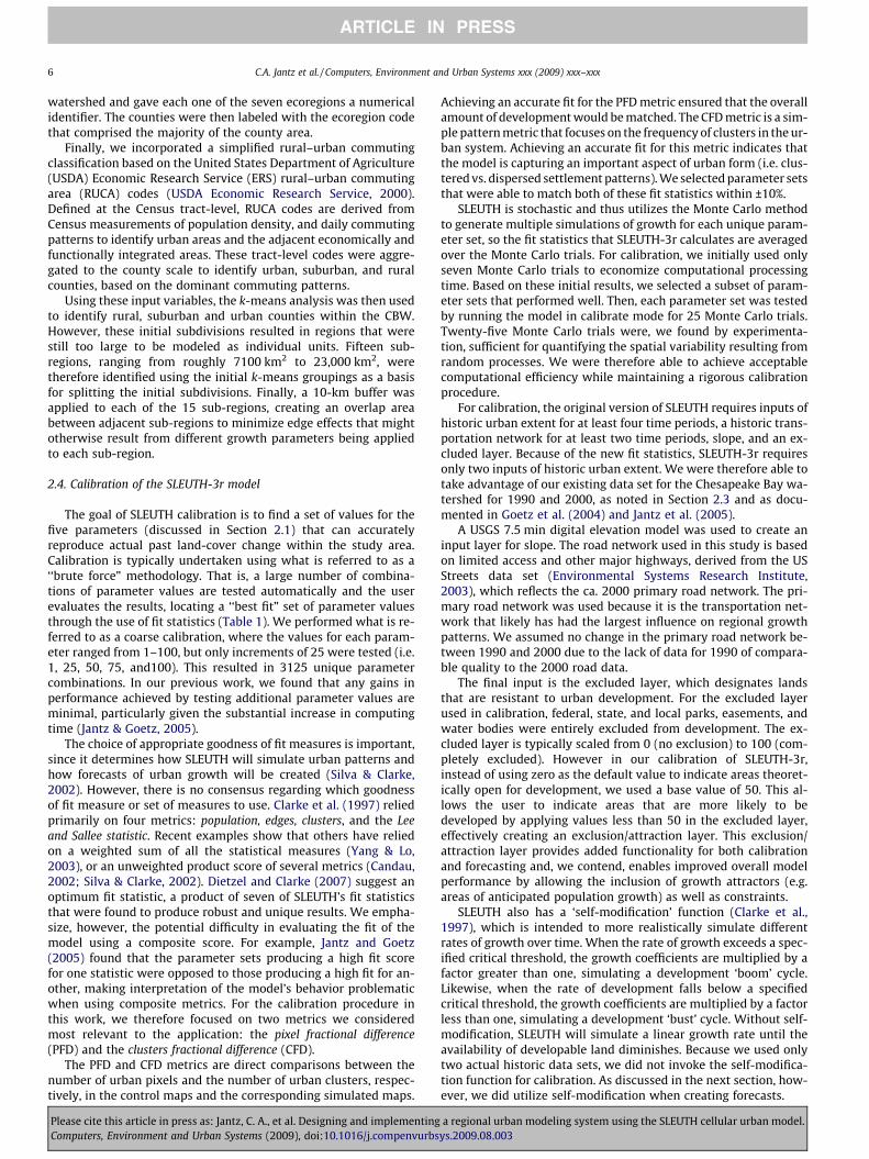
Table 2Input variables for multivariate k-means clustering. Variables were calculated for each co

Variable Data source

Percent developed area in 2000 Derived from 2000 impervious suMarks, 1995)

Area-weighted mean urban cluster size in 2000 Derived from 2000 impervious suMarks, 1995)

Urban cluster density in 2000 Derived from 2000 impervious suMarks, 1995)

Urban edge pixel density in 2000 Derived from 2000 impervious suMarks, 1995)

Population density in 2000 US Bureau of the Census (2000)Dominant rural–urban commuting classification

in 2000USDA Economic Research Service

1990–2000 Change in percent developed area Derived from 1990 and 2000 imp(McGarigal & Marks, 1995)

1990–2000 Change in area-weighted meancluster size

Derived from 1990 and 2000 imp(McGarigal & Marks, 1995)

1990–2000 Change in urban cluster density Derived from 1990 and 2000 imp(McGarigal & Marks, 1995)

1990–2000 Change in urban edge pixel density Derived from 1990 and 2000 imp(McGarigal & Marks, 1995)

1990–2000 Change in population density US Bureau of the Census (1990), UDominant ecoregion US Environmental Protection Agen


across the Chesapeake Bay watershed while maintaining the highspatial resolution of the available urban land cover maps. The ur-ban land cover data consist of maps of impervious surface cover,derived from Landsat TM and ETM + imagery, which capturedurbanization patterns between 1990 and 2000 (Goetz et al.,2004; Jantz et al., 2005). Urbanization in the region, as character-ized in the Landsat maps, was primarily associated with existingurban centers, such as Washington, DC, Baltimore, MD, and Nor-folk, VA. In many exurban counties, however, rates of change ex-ceed those in urban areas (Jantz et al., 2005). In addition,urbanization patterns in urban and suburban counties tend to becharacterized by clustered, high-density development. In exurbancounties development patterns tend to be more dispersed.

Because SLEUTH’s growth coefficients are applied globally with-in a study area, the heterogeneous urbanization patterns observedacross the Chesapeake Bay watershed, as well its size, required thatthe study area be subdivided; an analogous problem was faced bySoares-Filho et al. (2006) in the Amazon region. We used k-meanscluster analysis, a robust method for identifying groupings within adata set where within-group variability is minimized and be-tween-group variability is maximized (Aldenderfer & Blashfield,1984), to characterize rural, suburban and urban landscapes atthe county scale. These broad groups were then subdivided furtherinto smaller intermediate sub-regions, based on a combination ofpolitical boundaries, rural–urban commuting patterns, and physio-graphic provinces.

The cluster analysis was performed using the 208 counties thatintersect the Chesapeake Bay watershed and each county wascategorized as being rural, suburban or urban based on severalvariables, which are briefly discussed here and summarized inTable 2. Fragstats (version 3.3, build 4) (McGarigal & Marks,1995), a pattern analysis software package, was used to calculatecounty-level pattern metrics from the 2000 urban land covermap: percent area developed, area-weighted mean urban cluster(patch) size, urban edge pixel density and urban cluster density.Population density was derived from US Census data (US Bureauof the Census, 2000). The following measures of change between1990 and 2000 were also included: change in percent area devel-oped, change in urban cluster density, change in area-weightedmean urban cluster size, change in urban edge pixel density andthe percent change in population.

We also used the level-III EPA ecoregions (US EnvironmentalProtection Agency, 2003) that comprise the Chesapeake Bay

unty.

rface map (Goetz et al., 2004; Jantz et al., 2005) using FRAGSTATS (McGarigal &




(2000)

ervious surface maps (Goetz et al., 2004; Jantz et al., 2005) using FRAGSTATS




S Bureau of the Census (2000)cy (2003)




ARTICLE IN PRESS

watershed and gave each one of the seven ecoregions a numericalidentifier. The counties were then labeled with the ecoregion codethat comprised the majority of the county area.

Finally, we incorporated a simplified rural–urban commutingclassification based on the United States Department of Agriculture(USDA) Economic Research Service (ERS) rural–urban commutingarea (RUCA) codes (USDA Economic Research Service, 2000).Defined at the Census tract-level, RUCA codes are derived fromCensus measurements of population density, and daily commutingpatterns to identify urban areas and the adjacent economically andfunctionally integrated areas. These tract-level codes were aggre-gated to the county scale to identify urban, suburban, and ruralcounties, based on the dominant commuting patterns.

Using these input variables, the k-means analysis was then usedto identify rural, suburban and urban counties within the CBW.However, these initial subdivisions resulted in regions that werestill too large to be modeled as individual units. Fifteen sub-regions, ranging from roughly 7100 km2 to 23,000 km2, weretherefore identified using the initial k-means groupings as a basisfor splitting the initial subdivisions. Finally, a 10-km buffer wasapplied to each of the 15 sub-regions, creating an overlap areabetween adjacent sub-regions to minimize edge effects that mightotherwise result from different growth parameters being appliedto each sub-region.

2.4. Calibration of the SLEUTH-3r model

The goal of SLEUTH calibration is to find a set of values for thefive parameters (discussed in Section 2.1) that can accuratelyreproduce actual past land-cover change within the study area.Calibration is typically undertaken using what is referred to as a‘‘brute force” methodology. That is, a large number of combina-tions of parameter values are tested automatically and the userevaluates the results, locating a ‘‘best fit” set of parameter valuesthrough the use of fit statistics (Table 1). We performed what is re-ferred to as a coarse calibration, where the values for each param-eter ranged from 1–100, but only increments of 25 were tested (i.e.1, 25, 50, 75, and100). This resulted in 3125 unique parametercombinations. In our previous work, we found that any gains inperformance achieved by testing additional parameter values areminimal, particularly given the substantial increase in computingtime (Jantz & Goetz, 2005).

The choice of appropriate goodness of fit measures is important,since it determines how SLEUTH will simulate urban patterns andhow forecasts of urban growth will be created (Silva & Clarke,2002). However, there is no consensus regarding which goodnessof fit measure or set of measures to use. Clarke et al. (1997) reliedprimarily on four metrics: population, edges, clusters, and the Leeand Sallee statistic. Recent examples show that others have reliedon a weighted sum of all the statistical measures (Yang & Lo,2003), or an unweighted product score of several metrics (Candau,2002; Silva & Clarke, 2002). Dietzel and Clarke (2007) suggest anoptimum fit statistic, a product of seven of SLEUTH’s fit statisticsthat were found to produce robust and unique results. We empha-size, however, the potential difficulty in evaluating the fit of themodel using a composite score. For example, Jantz and Goetz(2005) found that the parameter sets producing a high fit scorefor one statistic were opposed to those producing a high fit for an-other, making interpretation of the model’s behavior problematicwhen using composite metrics. For the calibration procedure inthis work, we therefore focused on two metrics we consideredmost relevant to the application: the pixel fractional difference(PFD) and the clusters fractional difference (CFD).

The PFD and CFD metrics are direct comparisons between thenumber of urban pixels and the number of urban clusters, respec-tively, in the control maps and the corresponding simulated maps.


Achieving an accurate fit for the PFD metric ensured that the overallamount of development would be matched. The CFD metric is a sim-ple pattern metric that focuses on the frequency of clusters in the ur-ban system. Achieving an accurate fit for this metric indicates thatthe model is capturing an important aspect of urban form (i.e. clus-tered vs. dispersed settlement patterns). We selected parameter setsthat were able to match both of these fit statistics within ±10%.

SLEUTH is stochastic and thus utilizes the Monte Carlo methodto generate multiple simulations of growth for each unique param-eter set, so the fit statistics that SLEUTH-3r calculates are averagedover the Monte Carlo trials. For calibration, we initially used onlyseven Monte Carlo trials to economize computational processingtime. Based on these initial results, we selected a subset of param-eter sets that performed well. Then, each parameter set was testedby running the model in calibrate mode for 25 Monte Carlo trials.Twenty-five Monte Carlo trials were, we found by experimenta-tion, sufficient for quantifying the spatial variability resulting fromrandom processes. We were therefore able to achieve acceptablecomputational efficiency while maintaining a rigorous calibrationprocedure.

For calibration, the original version of SLEUTH requires inputs ofhistoric urban extent for at least four time periods, a historic trans-portation network for at least two time periods, slope, and an ex-cluded layer. Because of the new fit statistics, SLEUTH-3r requiresonly two inputs of historic urban extent. We were therefore able totake advantage of our existing data set for the Chesapeake Bay wa-tershed for 1990 and 2000, as noted in Section 2.3 and as docu-mented in Goetz et al. (2004) and Jantz et al. (2005).

A USGS 7.5 min digital elevation model was used to create aninput layer for slope. The road network used in this study is basedon limited access and other major highways, derived from the USStreets data set (Environmental Systems Research Institute,2003), which reflects the ca. 2000 primary road network. The pri-mary road network was used because it is the transportation net-work that likely has had the largest influence on regional growthpatterns. We assumed no change in the primary road network be-tween 1990 and 2000 due to the lack of data for 1990 of compara-ble quality to the 2000 road data.

The final input is the excluded layer, which designates landsthat are resistant to urban development. For the excluded layerused in calibration, federal, state, and local parks, easements, andwater bodies were entirely excluded from development. The ex-cluded layer is typically scaled from 0 (no exclusion) to 100 (com-pletely excluded). However in our calibration of SLEUTH-3r,instead of using zero as the default value to indicate areas theoret-ically open for development, we used a base value of 50. This al-lows the user to indicate areas that are more likely to bedeveloped by applying values less than 50 in the excluded layer,effectively creating an exclusion/attraction layer. This exclusion/attraction layer provides added functionality for both calibrationand forecasting and, we contend, enables improved overall modelperformance by allowing the inclusion of growth attractors (e.g.areas of anticipated population growth) as well as constraints.

SLEUTH also has a ‘self-modification’ function (Clarke et al.,1997), which is intended to more realistically simulate differentrates of growth over time. When the rate of growth exceeds a spec-ified critical threshold, the growth coefficients are multiplied by afactor greater than one, simulating a development ‘boom’ cycle.Likewise, when the rate of development falls below a specifiedcritical threshold, the growth coefficients are multiplied by a factorless than one, simulating a development ‘bust’ cycle. Without self-modification, SLEUTH will simulate a linear growth rate until theavailability of developable land diminishes. Because we used onlytwo actual historic data sets, we did not invoke the self-modifica-tion function for calibration. As discussed in the next section, how-ever, we did utilize self-modification when creating forecasts.




ARTICLE IN PRESS

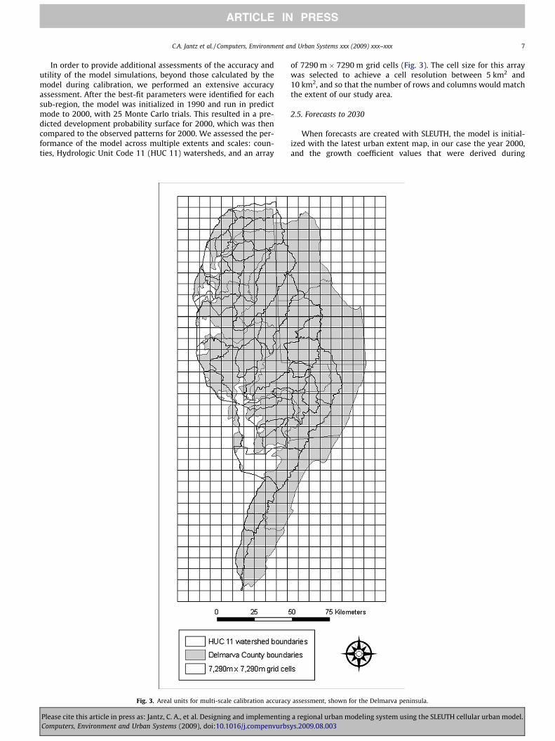
In order to provide additional assessments of the accuracy andutility of the model simulations, beyond those calculated by themodel during calibration, we performed an extensive accuracyassessment. After the best-fit parameters were identified for eachsub-region, the model was initialized in 1990 and run in predictmode to 2000, with 25 Monte Carlo trials. This resulted in a pre-dicted development probability surface for 2000, which was thencompared to the observed patterns for 2000. We assessed the per-formance of the model across multiple extents and scales: coun-ties, Hydrologic Unit Code 11 (HUC 11) watersheds, and an array

Fig. 3. Areal units for multi-scale calibration accuracy


of 7290 m � 7290 m grid cells (Fig. 3). The cell size for this arraywas selected to achieve a cell resolution between 5 km2 and10 km2, and so that the number of rows and columns would matchthe extent of our study area.

2.5. Forecasts to 2030

When forecasts are created with SLEUTH, the model is initial-ized with the latest urban extent map, in our case the year 2000,and the growth coefficient values that were derived during

assessment, shown for the Delmarva peninsula.




ARTICLE IN PRESS

calibration. The user sets the target year in which to stop theforecast; in our case we chose the year 2030. As in calibration,25 Monte Carlo trials were performed and each sub-region wasmodeled separately. For the forecasts presented here, we utilizedthe same exclusion/attraction layer that was used for calibration,

Fig. 4. Forecast scenario maps (exclusion/attr


assuming no change in spatial factors that would influence urbanpatterns in the future. For most sub-regions, we assumed a lineargrowth trend and thus did not invoke the model’s self-modificationfunctionality. However, for urban sub-regions, such as theWashington, DC–Baltimore, MD region, or urbanizing sub-regions,

action layers) for southeast Pennsylvania.




ARTICLE IN PRESS

such as the Delmarva Peninsula, the maintenance of linear growthrates was thought to be an implausible assumption. As landavailable for urbanization decreases, actual growth rates will slowas there is a greater economic incentive for growth to occur indenser clusters. Thus for these sub-regions, we allowed the model’s‘‘bust” self-modification to operate, using a multiplier of 0.95.When the model enters into the ‘‘bust” cycle, the self-modificationmultiplier is applied to the diffusion, breed, and spread coefficientvalues before each annual growth cycle begins, effectively lower-ing those values and slowing growth.

To illustrate the capability of SLEUTH to simulate alternativescenarios, we developed three different scenarios to forecast futuredevelopment for the southeast Pennsylvania sub-region, an area ofexpanding population and exurban growth (Fig. 1). This sub-regionis a good case study area because it has a large urban center, Har-risburg, PA, several small urban centers, such as Lancaster andYork, PA, and a heterogeneous exurban landscape that includesagricultural valleys and forested ridges. In addition, it is a regionthat has been experiencing rapid growth in recent years due toits proximity to the Washington, DC–Baltimore, MD and Philadel-phia, PA metropolitan regions.

For the test sub-region, alternative scenarios were implementedby developing exclusion/attraction layers that reflect different landuse policy scenarios (e.g. Jantz et al., 2004). In our case, we devel-oped three scenarios (Fig. 4):

1. A ‘‘business as usual” (BAU) scenario that assumed no change inthe excluded layer.

2. A trend scenario developed by the Chesapeake Bay Program (CBPtrend) that incorporates an agricultural vulnerability model. Inaddition to using the existing protected lands to designate areasthat are off-limits for new development, this scenario identifiescounty agricultural lands that are either more or less likely tobe developed based on the relative difference between the extentof modeled agricultural lands in 2030 and mapped agriculturallands in 2002 at the county scale (R. Burgholzer, pers. comm.,based on participation in the CBP Agricultural and NutrientReduction Workgroup). Because we calibrated SLEUTH using anexclusion/attraction layer with a base value of 50, county agricul-tural lands that are less likely to be developed were given a value

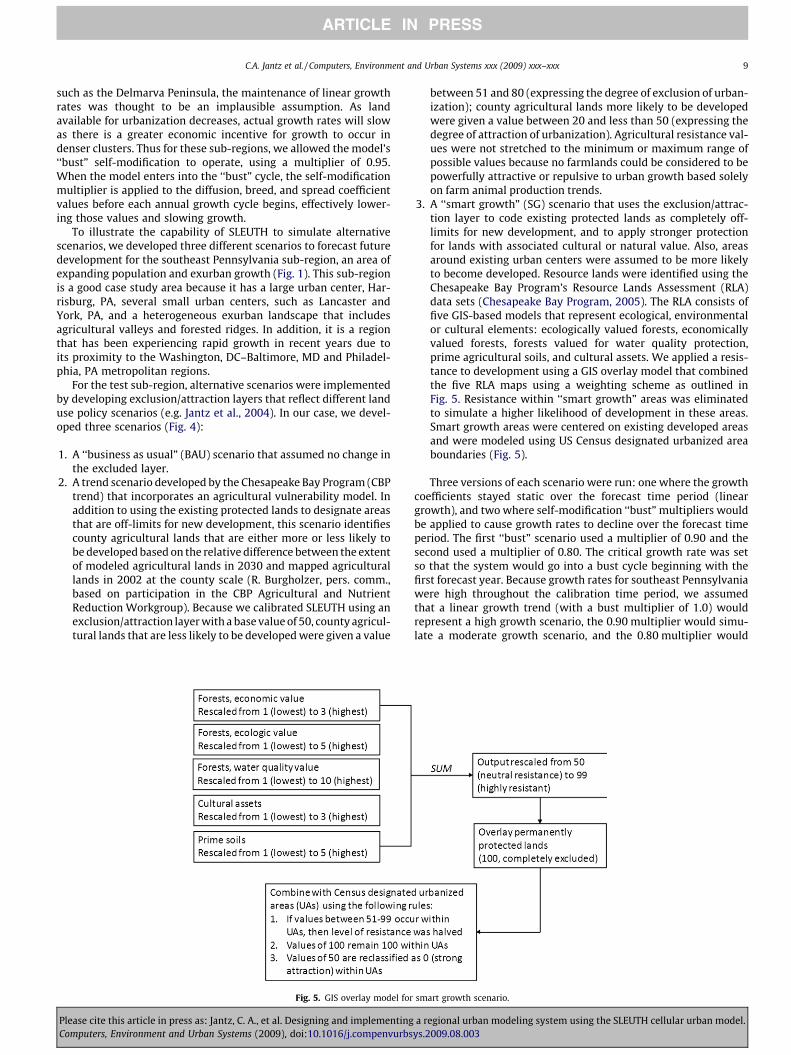
Fig. 5. GIS overlay model for


between 51 and 80 (expressing the degree of exclusion of urban-ization); county agricultural lands more likely to be developedwere given a value between 20 and less than 50 (expressing thedegree of attraction of urbanization). Agricultural resistance val-ues were not stretched to the minimum or maximum range ofpossible values because no farmlands could be considered to bepowerfully attractive or repulsive to urban growth based solelyon farm animal production trends.

3. A ‘‘smart growth” (SG) scenario that uses the exclusion/attrac-tion layer to code existing protected lands as completely off-limits for new development, and to apply stronger protectionfor lands with associated cultural or natural value. Also, areasaround existing urban centers were assumed to be more likelyto become developed. Resource lands were identified using theChesapeake Bay Program’s Resource Lands Assessment (RLA)data sets (Chesapeake Bay Program, 2005). The RLA consists offive GIS-based models that represent ecological, environmentalor cultural elements: ecologically valued forests, economicallyvalued forests, forests valued for water quality protection,prime agricultural soils, and cultural assets. We applied a resis-tance to development using a GIS overlay model that combinedthe five RLA maps using a weighting scheme as outlined inFig. 5. Resistance within ‘‘smart growth” areas was eliminatedto simulate a higher likelihood of development in these areas.Smart growth areas were centered on existing developed areasand were modeled using US Census designated urbanized areaboundaries (Fig. 5).

Three versions of each scenario were run: one where the growthcoefficients stayed static over the forecast time period (lineargrowth), and two where self-modification ‘‘bust” multipliers wouldbe applied to cause growth rates to decline over the forecast timeperiod. The first ‘‘bust” scenario used a multiplier of 0.90 and thesecond used a multiplier of 0.80. The critical growth rate was setso that the system would go into a bust cycle beginning with thefirst forecast year. Because growth rates for southeast Pennsylvaniawere high throughout the calibration time period, we assumedthat a linear growth trend (with a bust multiplier of 1.0) wouldrepresent a high growth scenario, the 0.90 multiplier would simu-late a moderate growth scenario, and the 0.80 multiplier would

smart growth scenario.




ARTICLE IN PRESS

simulate a low growth scenario. Thus, a total of nine forecast sce-narios were run, a low, medium and high growth forecast for eachof the three policy scenarios.

3. Results


The ability to interactively set a diffusion coefficient multiplierthat reflects the unique characteristics of the study area is a keyadvancement in the SLEUTH-3r model. For all sub-regions we wereable to identify a value for the diffusion coefficient multiplier thatwould over-estimate the number of urban clusters (by roughly30%) when diffusion growth was maximized (Table 3). This en-sured that SLEUTH-3r would be able to simulate an appropriate le-vel of diffusion growth (see Section 3.3 for calibration results).

Our modifications of the SLEUTH code to speed-up processingand to reduce memory requirements proved effective. The net

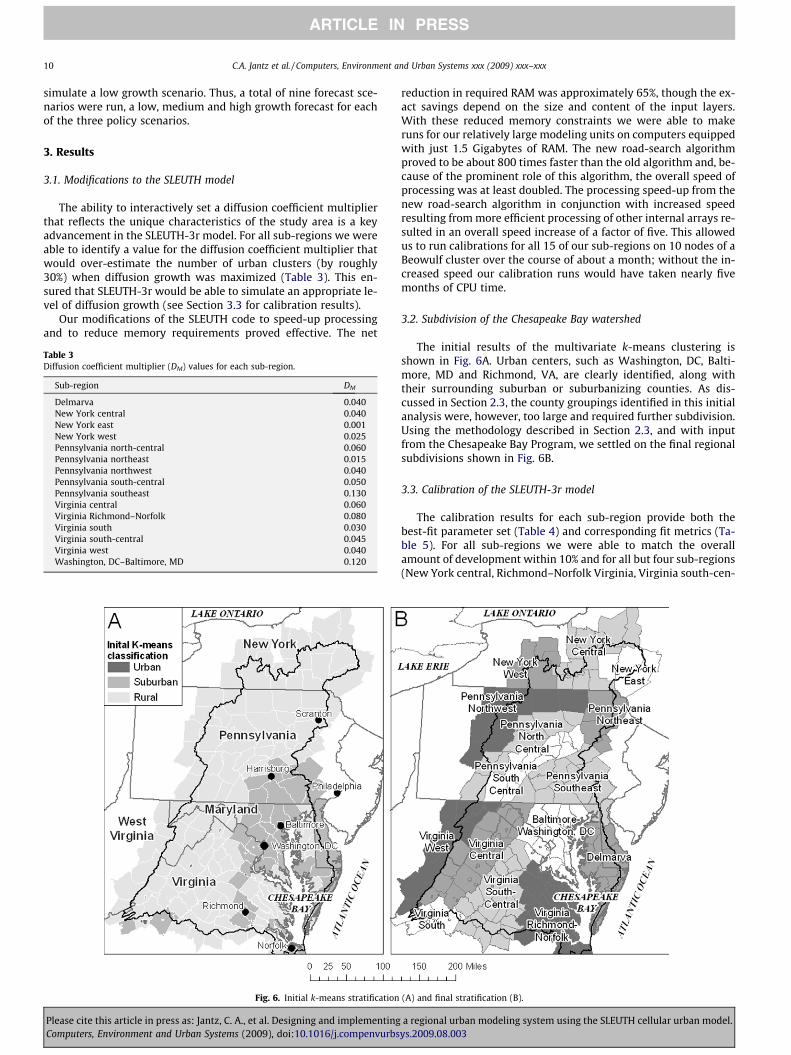
Fig. 6. Initial k-means stratification

Table 3Diffusion coefficient multiplier (DM) values for each sub-region.

Sub-region DM

Delmarva 0.040New York central 0.040New York east 0.001New York west 0.025Pennsylvania north-central 0.060Pennsylvania northeast 0.015Pennsylvania northwest 0.040Pennsylvania south-central 0.050Pennsylvania southeast 0.130Virginia central 0.060Virginia Richmond–Norfolk 0.080Virginia south 0.030Virginia south-central 0.045Virginia west 0.040Washington, DC–Baltimore, MD 0.120


reduction in required RAM was approximately 65%, though the ex-act savings depend on the size and content of the input layers.With these reduced memory constraints we were able to makeruns for our relatively large modeling units on computers equippedwith just 1.5 Gigabytes of RAM. The new road-search algorithmproved to be about 800 times faster than the old algorithm and, be-cause of the prominent role of this algorithm, the overall speed ofprocessing was at least doubled. The processing speed-up from thenew road-search algorithm in conjunction with increased speedresulting from more efficient processing of other internal arrays re-sulted in an overall speed increase of a factor of five. This allowedus to run calibrations for all 15 of our sub-regions on 10 nodes of aBeowulf cluster over the course of about a month; without the in-creased speed our calibration runs would have taken nearly fivemonths of CPU time.

3.2. Subdivision of the Chesapeake Bay watershed

The initial results of the multivariate k-means clustering isshown in Fig. 6A. Urban centers, such as Washington, DC, Balti-more, MD and Richmond, VA, are clearly identified, along withtheir surrounding suburban or suburbanizing counties. As dis-cussed in Section 2.3, the county groupings identified in this initialanalysis were, however, too large and required further subdivision.Using the methodology described in Section 2.3, and with inputfrom the Chesapeake Bay Program, we settled on the final regionalsubdivisions shown in Fig. 6B.


The calibration results for each sub-region provide both thebest-fit parameter set (Table 4) and corresponding fit metrics (Ta-ble 5). For all sub-regions we were able to match the overallamount of development within 10% and for all but four sub-regions(New York central, Richmond–Norfolk Virginia, Virginia south-cen-

(A) and final stratification (B).




ARTICLE IN PRESS

tral and Virginia south) we achieved a match within 5%. Likewise,for matching the number of urban clusters, all sub-regions exceptfor New York east achieved a match within 10% and most werematched within 5%.

SLEUTH calculates the fit metrics globally for each sub-region.We also present results of the model’s performance at the countyscale, HUC 11 watershed scale, and using the 7290 m � 7290 m lat-tice. Table 6 shows the results of linear regression analyses thatcompare the observed and simulated development in 2000 and ur-ban land-cover change between 1990 and 2000 for each areal unit.Fig. 7 illustrates, for the 7290 � 7290 lattice, the spatial patterns ofthe differences between simulated and observed urban land coverestimates for 2000.


The basin-wide forecasts (Fig. 8) indicate a continuation andintensification of development trends that were observed in the1990–2000 time period (Jantz et al., 2005). We note, for example,the intensification of urbanization in southeast Pennsylvania, be-tween Harrisburg and Philadelphia, and on the Delmarva Penin-

Table 4Parameter sets for each sub-region.

Sub-region Diffusion Breed

Delmarva 100 75New York central 50 25New York east 50 50New York west 100 50Pennsylvania north-central 75 25Pennsylvania northeast 100 50Pennsylvania northwest 75 50Pennsylvania south-central 50 50Pennsylvania southeast 75 75Virginia central 100 25Virginia Richmond–Norfolk 100 100Virginia south 50 50Virginia south-central 75 25Virginia west 75 1Washington, DC–Baltimore, MD 100 50

Table 5Calibration accuracy results for each sub-region. The number of urban pixels and the percensimulated number of pixels and clusters for 2000. For the pixels and clusters fractional dobserved data sets. Negative values indicate underestimation; positive values indicate ove

Sub-region 1990 Pixels(% urban)

2000 Pixels(% urban)

2000Simulatedpixels

Pixeldiffer

Delmarva 327,589 (0.80) 798,168 (1.96) 789,505 �0.0New York central 521,977 (0.85) 842,267 (1.37) 766,146 �0.0New York east 35,300 (0.14) 83,827 (0.34) 84,244 0.0New York west 214,957 (1.03) 432,758 (2.07) 425,102 �0.0Pennsylvania north-

central236,622 (0.32) 394,575 (0.54) 377,223 �0.0

Pennsylvanianortheast

229,234 (1.01) 370,372 (1.63) 384,873 0.0

Pennsylvanianorthwest

123,451 (0.18) 286,435 (0.42) 280,295 �0.0

Pennsylvania south-central

235,264 (0.45) 418,710 (0.80) 406,840 �0.0

Pennsylvaniasoutheast

1354,671 (2.34) 2045,556 (3.53) 2024,113 �0.0

Virginia central 197,389 (0.25) 495,483 (0.63) 502,965 0.0Virginia Richmond–

Norfolk1037,356 (1.86) 1608,125 (2.88) 1507,658 �0.0

Virginia south 102,681 (0.44) 289,000 (1.24) 262,528 �0.0Virginia south-central 142,646 (0.24) 467,646 (0.79) 494,381 0.0Virginia west 75,543 (0.10) 226,422 (0.29) 219,623 �0.0Washington, DC–

Baltimore, MD2211,517 (4.53) 3031,176 (6.21) 2973,476 �0.0


sula. Likewise, exurban development throughout Virginia is alsoapparent.

The results for the nine 2030 forecasts for southeast Pennsylva-nia (Fig. 9) indicate that the overall amount of development be-tween the BAU and SG scenarios, regardless of the growth rates,was similar. Fig. 10 focuses on these two scenarios to illustratethe spatial differences in growth patterns. The CBP trend scenarioconsistently resulted in higher levels of growth, likely due to thefact that there are more pixels available for urbanization in thisscenario. As an example of an impact assessment, we comparedthe types of land converted to development by overlaying the fore-cast maps with the RLA map developed for the smart growth sce-nario (Fig. 11).

4. Discussion


The added functionality of SLEUTH-3r has greatly enhanced themodel’s ability to capture urbanization patterns across a widerange of conditions. That we found diffusion coefficient multiplier

Spread Slope Road growth

50 25 5025 50 50

100 50 2550 100 2525 1 7575 100 5050 25 125 50 5025 1 5050 25 2525 75 2550 100 5075 50 5075 50 125 1 50

t urban, and the number of urban clusters for 1990 and 2000 are given, along with theifference metrics, a zero value indicates a perfect match between the simulated andrestimation.

s fractionalence

1990Clusters

2000Clusters

2000 Simulatedclusters

Clusters fractionaldifference

1 92,427 185,299 166,896 �0.099 75,436 126,166 119,151 �0.050 9840 25,361 9831 �0.601 51,886 89,171 88,390 �0.014 48,243 85,696 85,090 �0.01

4 32,121 56,535 55,482 �0.02

2 29,886 70,959 71,381 0.01

2 57,983 109,305 102,917 �0.05

1 248,499 349,571 315,144 �0.09

2 45,043 118,785 129,152 0.086 124,248 203,814 213,845 0.04

9 18,828 62,161 56,182 �0.096 35,359 122,487 121,610 �0.013 23,871 65,167 68,078 0.001 229,441 299,615 275,798 �0.07



Table 6Calibration accuracy results for counties, HUC 11 watersheds, and an array of 7290 � 7290 m grid cells. Ordinary least squares (OLS) regression scores are presented for bothestimates of total developed area and for estimates of change in developed area between 1990 and 2000.

Estimated developed area (r2) Estimated change in developed area, 1990–2000 (r2)

Counties, N = 208 0.97, p < 0.01 0.74, p < 0.01HUC 11 watersheds, N = 505 0.98, p < 0.01 0.65, p < 0.017290 � 7290 lattice, N = 5126 0.97, p < 0.01 0.74, p < 0.01

Fig. 7. Difference in estimates of percentage developed area, where the simulated estimates were subtracted from the mapped estimates. Negative values thus represent thatSLEUTH-3d is under-estimating development in 2000, while positive values represent an overestimation.


ARTICLE IN PRESS

Please cite this article in press as: Jantz, C. A., et al. Designing and implementing a regional urban modeling system using the SLEUTH cellular urban model.Computers, Environment and Urban Systems (2009), doi:10.1016/j.compenvurbsys.2009.08.003



ARTICLE IN PRESS

values ranging from 0.001 to 0.130 for the Chesapeake Bay wa-tershed sub-regions (Table 3), illustrates both the heterogeneityof urbanization patterns found in the study area and the model’snew ability to adapt to these conditions. While it is outside thescope of this paper to address how these patterns may reflect the

Fig. 9. Forecast results for southea

Fig. 8. Basin-wide forecasts to 2030. The percentage of each county’s area that is


process of urban growth, the diffusion multiplier could offer newinsight into these questions. The new fit metrics enable applicationof SLEUTH-3r in areas that lack more than two data sets represent-ing historic urban land cover. We found the fractional differencemetrics (PFD, CFD) particularly useful because they quantified both

st Pennsylvania, 2000–2030.

urbanized in 2000 is shown in (A), and the forecast for 2030 is shown in (B).



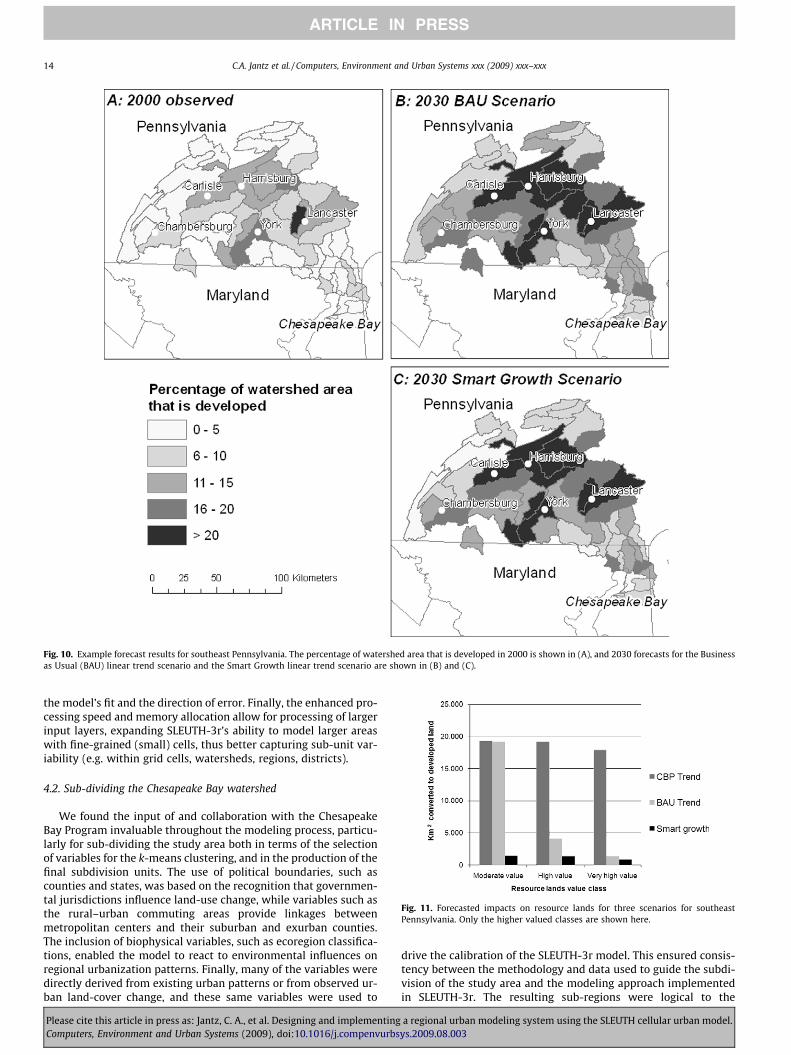
Fig. 10. Example forecast results for southeast Pennsylvania. The percentage of watershed area that is developed in 2000 is shown in (A), and 2030 forecasts for the Businessas Usual (BAU) linear trend scenario and the Smart Growth linear trend scenario are shown in (B) and (C).

Fig. 11. Forecasted impacts on resource lands for three scenarios for southeastPennsylvania. Only the higher valued classes are shown here.


ARTICLE IN PRESS

the model’s fit and the direction of error. Finally, the enhanced pro-cessing speed and memory allocation allow for processing of largerinput layers, expanding SLEUTH-3r’s ability to model larger areaswith fine-grained (small) cells, thus better capturing sub-unit var-iability (e.g. within grid cells, watersheds, regions, districts).

4.2. Sub-dividing the Chesapeake Bay watershed

We found the input of and collaboration with the ChesapeakeBay Program invaluable throughout the modeling process, particu-larly for sub-dividing the study area both in terms of the selectionof variables for the k-means clustering, and in the production of thefinal subdivision units. The use of political boundaries, such ascounties and states, was based on the recognition that governmen-tal jurisdictions influence land-use change, while variables such asthe rural–urban commuting areas provide linkages betweenmetropolitan centers and their suburban and exurban counties.The inclusion of biophysical variables, such as ecoregion classifica-tions, enabled the model to react to environmental influences onregional urbanization patterns. Finally, many of the variables weredirectly derived from existing urban patterns or from observed ur-ban land-cover change, and these same variables were used to


drive the calibration of the SLEUTH-3r model. This ensured consis-tency between the methodology and data used to guide the subdi-vision of the study area and the modeling approach implementedin SLEUTH-3r. The resulting sub-regions were logical to the




ARTICLE IN PRESS

Chesapeake Bay Program partners, a good indication of the prag-matic validity of our choice of 15 sub-regions.


The calibration results show wide variation in the best-fitparameters derived for each sub-region (Table 4), reinforcing thejustification for sub-dividing the study area. These results alsoindicate the sensitivity of the model to the input data. For example,the best score for the clusters fractional difference metric for theNew York east sub-region was –0.60, indicating a 60% underesti-mation (Table 5). This case reflects the poor quality of the 1990data for this sub-region (due to cloud cover in the original satelliteimagery) rather than the model’s inability to capture the observedurbanization rates and patterns. The performance of the model forthe other sub-regions was quite good at the aggregate level of thesub-regions (Table 5).

While the model also performs well at finer scales, trade-offs be-come apparent. In examining the difference between the amount ofurbanization estimated by the model and the observed urbanizationfor the year 2000 (Fig. 8), areas where the model consistently over-estimated tended to fall within the exurban or rural landscapes. Incontrast, the areas where the most significant underestimation oc-curred were associated with urban centers. This is particularly evi-dent for Richmond, VA, Washington, DC and Harrisburg, PA. Theseresults indicate the challenge of capturing local scale heterogeneityin densely developed areas. Nonetheless, we note that for nearly theentire CBW watershed we are able to capture the amount of urbandevelopment within 5%, which we feel are particularly positive re-sults given the scale and scope of this project.


The basin-wide forecasts presented here (Fig. 8) were createdbased on a set of assumptions that reflect ‘‘business as usual,” soit is not surprising that the results indicate an intensification of his-toric development patterns. These results do, however, provide animportant baseline from which alternative scenarios can be evalu-ated, both in terms of the spatial pattern of development, potentialimpacts on resource lands, and impacts on water quality andhydrology. These are on-going efforts at the time of this writing,as noted below in Section 5.

The forecasts presented for southeast Pennsylvania representexamples of how alternative future scenarios can be developed inSLEUTH-3r. The use of the exclusion/attraction layer and the useof self-modification to simulate high, medium and low growthrates, are innovations that warrant special attention in futureapplications. While we did not conduct quantitative sensitivityanalyses related to these innovations, we have demonstrated thatthe utility of this approach is both important and promising. Wewere able to evaluate alternative futures that exhibited similar lev-els of new development across sub-regions, but differed in terms ofthe spatial patterns of development and the types of land con-verted to new development (Figs. 7 and 8). These results can beused as input to other models to quantify impacts on, for example,water quality, flood risk, or wildlife habitat (e.g. Goetz, Jantz, &Jantz, 2009). It is precisely this type of information that is impor-tant for ecosystem management and sound land use decision-mak-ing (e.g. Jantz & Goetz, 2007).

5. Conclusion

This paper presents the broadest scale application of theSLEUTH model to date – a rare example of a fine-scale land-coverchange model applied across a large region – and introduces a


new version of SLEUTH with substantially augmented functional-ity. We have introduced new fit statistics that significantly en-hance the calibration process, and enable application of themodel when historic data are available for only two points in time.The use of relative exclusion/attraction values has expanded thecapability of SLEUTH to incorporate economic, cultural and policyinformation with bearing on historic and future urbanizationtrends (e.g. Jantz & Goetz, 2007). Taken together, all of thesechanges open up new avenues for the integration of SLEUTH withother land-change models (e.g. Goetz, Jantz, Towe, & Bockstael,2007). Future research will also be able to use the new informationgenerated by SLEUTH-3r to address questions related to how urbanpatterns relate to the process of urban land-cover change. In addi-tion, we have made significant advances in the model’s computa-tional efficiency.

The Chesapeake Bay Program is currently using the results fromSLEUTH-3r to prepare future land use inputs for their HydrologicSimulation Program-Fortran (HSPF) watershed model. Becausewe were able to preserve the high-resolution of the land coverdata, SLEUTH-3r provided the capability of visualizing alternativefuture scenarios at a detailed scale, which helped to engage stake-holders in the scenario development process. SLEUTH-3r and HSPFare especially good complements because HSPF, as a lumpedparameter model, tends to dampen and correct any absolute spa-tial errors in SLEUTH’s forecasts by aggregating results to broaderspatial scales (larger grain sizes).

We believe this project represents an important advancementin computational modeling of urban growth. In terms of simulationmodeling, we have presented several new advancements in theSLEUTH model’s performance and capabilities. More importantly,however, this project represents a successful broad scale modelingframework that has direct applications to land use management.

Acknowledgements

We acknowledge the support of the NASA Land Cover Land UseChange program (Grant NNG06GC43G to SJG), the EPA Science toAchieve Results program (Grant R82868401 to SJG), the US Geolog-ical Survey Geographic Analysis and Monitoring Program and theEPA Chesapeake Bay Program. We thank Rob Burgholzer for hisassistance in developing the CBP trend scenario, and William (Skip)Little for some of the initial SLEUTH code modifications. We alsothank Jules Opton-Himmel, Dan Steinberg and Greg Fiske at WHRC,and Kyle Shenk and Gary Lasako at Shippensburg University ofPennsylvania, for assistance with GIS data processing. We alsoacknowledge the helpful and constructive reviews provided byfour anonymous reviewers.

References

Aldenderfer, M. S., & Blashfield, R. K. (1984). Cluster analysis. Newberry Park, CA:Sage Publications.

Batty, M. (1997). Cellular automata and urban form: A primer. Journal of theAmerican Planning Association, 62, 266–275.

Candau, J. (2002). Temporal Calibration Sensitivity of the SLEUTH Urban Growth Model.MA thesis. Department of Geography, University of California, Santa Barbara,CA.

Chesapeake Bay Program (2000). Chesapeake 2000: A watershed partnership.<http://www.chesapeakebay.net/agreement.htm>.

Chesapeake Bay Program (2005). Resource lands assessment. <http://www.chesapeakebay.net/rla.htm>.

Clarke, K. C., Hoppen, S., & Gaydos, L. J. (1997). A self-modifying cellular automatonmodel of historical urbanization in the San Francisco Bay Area. Environment andPlanning B: Planning and Design, 24, 247–261.

Clarke, K. C., & Gaydos, L. J. (1998). Loose-coupling a cellular automaton model andGIS: Long-term urban growth prediction for San Francisco and Washington/Baltimore. International Journal of Geographical Information Science, 12, 699–714.

Couclelis, H. (1997). From cellular automata to urban models: New principles formodel development and implementation. Environment and Planning B: Planningand Design, 24, 165–174.


http://www.chesapeakebay.net/agreement.htm

http://www.chesapeakebay.net/rla.htm

http://www.chesapeakebay.net/rla.htm



ARTICLE IN PRESS

Dietzel, C., & Clarke, K. C. (2007). Toward optimal calibration of the SLEUTH land usechange model. Transactions in GIS, 11, 29–45.

Environmental Systems Research Institute. (2003). US streets (data set). Redlands,CA.

Goetz, S. J., Jantz, C. A., Prince, S. D., Smith, A. J., Varlyguin, D., & Wright, R. (2004).Integrated analysis of ecosystem interactions with land use change: TheChesapeake Bay watershed. In R. S. DeFries, G. P. Asner, & R. A. Houghton (Eds.),Ecosystems and land use change (pp. 263–275). Washington, DC: AmericanGeophysical Union.

Goetz, S. J., Jantz, C. A., Towe, C. A., Bockstael, N. (2007). Modeling the urbanizationprocess across Maryland in the context of Chesapeake Bay restoration.Conference Paper 06 Smart Growth @ 10. College Park, MD. <http://www.rff.org/rff/Events/SmartGrowthat10.cfm>.

Goetz, S. J., Jantz, P. A., & Jantz, C. A. (2009). Connectivity of core habitat in thenortheastern United States: Parks and protected areas in a landscape context.Remote Sensing of Environment, 113, 1421–1429.

Jantz, P. A., Goetz, S. J., & Jantz, C. A. (2005). Urbanization and the loss of resourcelands within the Chesapeake Bay watershed. Environmental Management, 36,343–360.

Jantz, C. A., & Goetz, S. J. (2007). Can smart growth save the Chesapeake Bay? Journalof Green Building, 2, 41–51.

Jantz, C. A., & Goetz, S. J. (2005). Analysis of scale dependencies in an urban land-use-change model. International Journal of Geographical Information Science, 19,217–241.

Jantz, C. A., Goetz, S. J., & Shelley, M. K. (2004). Using the SLEUTH urban growthmodel to simulate the impacts of future policy scenarios on urban land use inthe Baltimore–Washington metropolitan area. Environment and Planning B:Planning and Design, 31, 251–271.

Li, X., & Liu, X. (2006). An extended cellular automaton using case-based reasoningfor simulating urban development in a large complex region. InternationalJournal of Geographical Information Science, 20, 1109–1136.

McGarigal, K., Marks, B. J. (1995). FRAGSTATS: Spatial pattern analysis program forquantifying landscape structure. USDA Forest Service General Technical ReportPNW-351. <http://www.umass.edu/landeco/pubs/Fragstats.pdf>.

O’Sullivan, D., & Torrens, P. M. (2000). Cellular models of urban systems. In S.Bandini & T. Worsch (Eds.), Theoretical and practical issues on cellular automata(pp. 108–116). London: Springer.


Silva, E. A., & Clarke, K. C. (2002). Calibration of the SLEUTH urban growth model forLisbon and Porto, Spain. Computers, Environment and Urban Systems, 26,525–552.

Silva, E. A., & Clarke, K. C. (2005). Complexity, emergence and cellular urban models:Lessons learned from applying SLEUTH to two Portuguese metropolitan areas.European Planning Studies, 13, 93–116.

Soares-Filho, B. S., Nepstad, D. C., Curran, L. M., Cerqueira, G. C., Garcia, R. A., Ramos,C. A., et al. (2006). Modelling conservation in the Amazon Basin. Nature, 440,520–523.

Torrens, P. M. (2006). Simulating sprawl. Annals of the Association of AmericanGeographers, 96, 248–275.

Torrens, P. M., & O’Sullivan, D. (2001). Cellular automata and urban simulation:Where do we go from here? Environment and Planning B: Planning and Design,28, 163–168.

US Bureau of the Census (1990). Census 1990 summary file 1 (SF 1) 100-percentdata.

US Bureau of the Census (2000). Census 2000 summary file 1 (SF 1) 100-percentdata.

US Environmental Protection Agency (2003). Level III ecoregions of the conti-nental United States.<http://www.epa.gov/waterscience/basins/metadata/ecoreg.htm>.

US Geological Survey (2007). Project gigalopolis: Urban and land cover modeling.<http://www.ncgia.ucsb.edu/projects/gig/>.

USDA Economic Research Service (2000). 2000 rural–urban commuting area codes.<http://www.ers.usda.gov/Data/RuralUrbanCommutingAreaCodes/>.

Van Vliet, J., White, R., & Dragicevic, S. (2009). Modeling urban growth using avariable grid cellular automaton. Computers, Environment and Urban Systems, 33,35–43.

White, R., & Engelen, G. (1997). Cellular automata as the basis of integrated dynamicregional modelling. Environment and Planning B: Planning and Design, 24,235–246.

Yang, X., & Lo, C. P. (2003). Modelling urban growth and landscape changes in theAtlanta metropolitan area. International Journal of Geographical InformationScience, 17, 463–488.


http://www.rff.org/rff/Events/SmartGrowthat10.cfm

http://www.rff.org/rff/Events/SmartGrowthat10.cfm

http://www.umass.edu/landeco/pubs/Fragstats.pdf

http://www.epa.gov/waterscience/basins/metadata/ecoreg.htm

http://www.epa.gov/waterscience/basins/metadata/ecoreg.htm

http://www.ncgia.ucsb.edu/projects/gig/

http://www.ers.usda.gov/Data/RuralUrbanCommutingAreaCodes/


designing and implementing a regional urban modeling...

Documents