designing an anisotropic noise filter for measuring

Designing an Anisotropic Noise Filter for Measuring Critical Dimension and Line Edge

Roughness from SEM Images

by

Hyesung Ji

A thesis submitted to the Graduate Faculty of

Auburn University

in partial fulfillment of the

requirements for the Degree of

Master of Science

Auburn, Alabama

May, 5, 2018

Keywords: edge detection, anisotropic filter, SEM image, noise estimation

Copyright 2018 by Hyesung Ji

Approved by

Soo-Young Lee, Professor of Electrical and Computer Engineering

Bogdan M. Wilamowski, Professor of Electrical and Computer Engineering

Gopikrishna Deshpande, Associate Professor of Electrical and Computer Engineering

ii

Abstract

The scanning electron microscope (SEM) is often employed in inspecting patterns

transferred through a lithographic process. A typical inspection is to measure the critical

dimension (CD) and line edge roughness (LER) of each feature in a transferred pattern. Such

inspection may be done by utilizing image processing techniques to detect the boundaries of a

feature. Since SEM images tend to include a substantial level of noise, a proper reduction of

noise is essential before the subsequent process of edge detection. In a previous study, a method

of designing an isotropic Gaussian filter adaptive to the noise level was developed. However, its

performance for relatively small features was not so good as for large features, especially in the

case of LER. The main objective of this study is to improve the design method such that the

accuracy of the measured CD and LER is not deteriorated substantially as the feature size

decreases. The new design method allows a Gaussian filter to be anisotropic for the better

adaptability to the signal and noise, both of which show a substantial level of directional

correlation. The cut-off frequency for the direction normal to features is determined to include

most of the signal components and the cut-off frequency in the other direction is set to balance

between the signal and noise components to be included. This procedure enables a systematic

and easy design of the filter. Also, the method of estimating the noise has been modified for

higher accuracy. The performance of the anisotropic Gaussian filter designed by the new

method has been thoroughly analyzed using the reference images for which the CD and LER are

known. It is observed that the CD and LER errors have been significantly lowered, especially

for relatively small features.

iii

Acknowledgement

First of all, I would like to express my gratitude to my advisor Dr. Soo-Young Lee for

leading me into this exciting research area of proximity effect correction in electron beam

lithography and providing me with valuable support throughout my master program. Without his

detailed guidance and helpful suggestions this thesis would not have been possible. I thank him

for his patience and encouragement that carried me on through difficult times. I appreciate his

vast knowledge and skills in many areas that greatly contributed to my research and this thesis.

Special thanks are also given to the other members of my committee, Dr. Bogdan Wilamowski

and Dr. Gopikrishna Deshpande, for their valuable assistance and comments. I also benefited a

lot from the courses taught by them.

I would like to extend my gratitude to our research group. I would like to thank Dehua Li

and Soomin Moon for our memorable collaborations in the research. I also would like to extend

my gratitude to the Korea Army, which supported my study for two years.

Finally, I am greatly indebted to my parents, and elder sister, for their support to me

through my entire life, and in particular to my wife, Okkyeung Han, for her love, patience, and

understanding.

iv

Table of Contents

Abstract . . .. . . . . . . . . . . . . . . . . . . . . . . . . . . . . . . . . . . . . . . . . . . . . . . . . . . . . . . . . . . . . . . . ii

Acknowledgments . . . . . . . . . . . . . . . . . . . . . . . . . . . . . . . . . . . . . . . . . . . . . . . . . . . . . . . . . . iii

List of figures . . . . . . . . . . . . . . . . . . . . . . . . . . . . . . . . . . . . . . . . . . . . . . . . . . . . . . . . . . . . . . vi

List of Tables . . . . . . . . . . . . . . . . . . . . . . . . . . . . . . . . . . . . . . . . . . . . . . . . . . . . . . . . . . . . . . vii

1 Introduction . . . . . . . . . . . . . . . . . . . . . . . . . . . . . . . . . . . . . . . . . . . . . . . . . . . . . . . . . . 1

1.1 Problem definition . . . . . . . . . . . . . . . . . . . . . . . . . . . . . . . . . . . . . . . . . . . . . . . 1

1.2 Review of previous work . . . . . . . . . . . . . . . . . . . . . . . . . . . . . . . . . . . . . . . . . . 2

1.3 Motivation and objective . . . . . . . . . . . . . . . . . . . . . . . . . . . . . . . . . . . . . . . . . . 3

2 Analysis of SEM Image . . . . . . . . . . . . . . . . . . . . . . . . . . . . . . . . . . . . . . . . . . . . . . . . . 4

2.1 Feature boundaries. . . . . . . . . . . . . . . . . . . . . . . . . . . . . . . . . . . . . . . . . . . . . . . .5

2.2 Measurement of CD and LER . . . . . . . . . . . . . . . . . . . . . . . . . . . . . . . . . . . . . .6

2.3 Noise estimation . . . . . . . . . . . . . . . . . . . . . . . . . . . . . . . . . . . . . . . . . . . . . . . . .8

3 Filter Design. . . . . . . . . . . . . . . . . . . . . . . . . . . . . . . . . . . . . . . . . . . . . . . . . . . . . . . . . 12

3.1 Determination of cut-off frequencies . . . . . . . . . . . . . . . . . . . . . . . . . . . . . . . . 13

3.2 Boundary detection . . . . . . . . . . . . . . . . . . . . . . . . . . . . . . . . . . . . . . . . . . . . . .15

4 Results and Discussion . . . . . . . . . . . . . . . . . . . . . . . . . . . . . . . . . . . . . . . . . . . . . . . . .16

4.1 Reference images. . . . . . . . . . . . . . . . . . . . . . . . . . . . . . . . . . . . . . . . . . . . . . . .16

4.2 Comparison with the previous results . . . . . . . . . . . . . . . . . . . . . . . . . . . . . . . .17

4.3 The same type of noise as in SEM images . . . . . . . . . . . . . . . . . . . . . . . . . . . .19

v

4.4 Noise with horizontal correlation only . . . . . . . . . . . . . . . . . . . . . . . . . . . . . . 21

4.5 Noise with no spatial correlation. . . . . . . . . . . . . . . . . . . . . . . . . . . . . . . . . . . 22

4.6 Feature size . . . . . . . . . . . . . . . . . . . . . . . . . . . . . . . . . . . . . . . . . . . . . . . . . . . 24

5 Conclusion . . . . . . . . . . . . . . . . . . . . . . . . . . . . . . . . . . . . . . . . . . . . . . . . . . . . . . . . . .25

References . . . . . . . . . . . . . . . . . . . . . . . . . . . . . . . . . . . . . . . . . . . . . . . . . . . . . . . . . . . . . . . .27

vi

List of Figures

2.1 (a) An example of SEM image of L/S pattern and (b) the brightness distribution over a

feature boundary (black dashed lines show the locations of peak points and red dashed lines

show the locations of maximum-gradient points) . . . . . . . . . . . . . . . . . . . . . . . . . . . . . . . . . . . . . 4

2.2 (a) The detected inner and outer edges on the corresponding SEM image. (b) The inner and

outer edges in the resist profile. . . . . . . . . . . . . . . . . . . . . . . . . . . . . . . . . . . . . . . . . . . . . . . . . . . .5

2.3 (a) Line edge roughness and (b) the tilt angle estimated by fitting a straight line to the edge

points . . . . . . . . . . . . . . . . . . . . . . . . . . . . . . . . . . . . . . . . . . . . . . . . . . . . . . . . . . . . . . . . . . . . . . 7

2.4 (a) Flat regions are extracted from the SEM image and (b) the brightness distribution along a

cross-section of SEM image (regions between dashed lines are flat regions) . . . . . . . . . . . . . . . 8

2.5 The brightness distribution along the direction normal to line features after Gaussian

filtering . . . . . . . . . . . . . . . . . . . . . . . . . . . . . . . . . . . . . . . . . . . . . . . . . . . . . . . . . . . . . . . . . . . . . 10

2.6 (a) The brightness distribution before (top) and after (bottom) the filtering and (b) the

gradient of brightness distribution before (top) and after (bottom) the filtering . . . . . . . . . . . . . 10

3.1 (a) The signal and noise spectra along the direction perpendicular to lines. (b) The signal and

noise spectra along the direction parallel with lines . . . . . . . . . . . . . . . . . . . . . . . . . . . . . . . . . . 12

3.2 An example of magnified SEM image: (a) after and (b) before filtering . . . . . . . . . . . . . . . 14

3.3 The detected edges are overlaid with the corresponding SEM image . . . . . . . . . . . . . . . . . 15

4. 1 An example of the reference SEM image . . . . . . . . . . . . . . . . . . . . . . . . . . . . . . . . . . . . . . 16

vii

List of Tables

4.1 The known LER and CD in the six reference images . . . . . . . . . . . . . . . . . . . . . . . . . . . . . . 17

4.2 Comparison between the isotropic filter designed by the previous method and the anisotropic

filter designed by the new method for the reference images with the target line-width of 60nm,

and horizontally and vertically correlated noise . . . . . . . . . . . . . . . . . . . . . . . . . . . . . . . . . . . . . 18

4.3 Comparison between the isotropic and anisotropic filters designed by the new method for the reference

images with the target line-width of 120nm, and horizontally and vertically correlated noise . . . . . . . . . 19


images with the target line-width of 60nm, and horizontally and vertically correlated noise . . . . . . . . . . 20


images with the target line-width of 50nm, and horizontally and vertically correlated noise . . . . . . . . . . 20

4.6 Comparison between the isotropic and anisotropic filters designed by the new method for the

reference images with the target line-width of 120nm, and horizontally correlated noise. . . . . . 21


reference images with the target line-width of 60nm, and horizontally correlated noise. . . . . . . 21


reference images with the target line-width of 120nm, and horizontally correlated noise. . . . . . 22

viii


reference images with the target line-width of 120nm, and noise with no spatial correlation . . . 22


reference images with the target line-width of 60nm, and noise with no spatial correlation . . . . 23


reference images with the target line-width of 50nm, and noise with no spatial correlation . . . . 23

4.12 The average CD and LER errors for each target line-width . . . . . . . . . . . . . . . . . . . . . . . . 24

4.13 The averaged filter size for each target line-width . . . . . . . . . . . . . . . . . . . . . . . . . . . . . . . 24

1

Chapter 1

Introduction

Semiconductor devices are fabricated by transferring the corresponding circuit patterns

onto substrates using various lithographic processes such as electron-beam lithography [1-5]. A

circuit pattern is written on the resist layer of a substrate system and the resist is developed

subsequently. It is often required to inspect the fidelity of the written pattern on the resist [6-7].

An inspection method widely used is to take a SEM (scanning electron microscope) image of the

written pattern and analyze it to measure certain metrics such as the critical dimension (CD) and

line edge roughness (LER) of a circuit feature [6-7]. One of the analysis procedures is to employ

image processing techniques by which the boundaries of features are detected and compute the

CD and LER from the boundaries [7]. Since SEM images tend to be noisy, it is essential to

reduce the noise level before the boundary (edge) detection is carried out. This thesis addresses

the issue of designing a noise filter.

1.1. Problem definition

The noise filtering has a direct effect on the accuracy of boundary detection and therefore

it is critical to employ a noise filter optimized for the detection of feature boundaries in SEM

images [7]. One of the characteristics specific to typical SEM images, which may be taken into

account in designing a noise filter, is that features in a circuit pattern tend to have a certain

2

spatial orientation as in a line/space (L/S) pattern [8,10,11,12]. The power spectral density of

SEM image of such features shows a different distribution in the direction of orientation,

compared to the direction normal to the orientation. Another characteristic is that the noise in a

SEM image exhibits a spatial correlation in the direction of beam scanning. Hence, the power

spectral density of noise has a broader distribution in the corresponding direction. In addition,

the power spectral densities of features and noise vary with SEM image. The specific problem

studied in this research is how to design a noise filter which exploits these characteristics in order

to enable detecting feature boundaries accurately.

1.2. Review of previous work

A fixed filter, e.g., median or spatial averaging filter, may be considered [7-15], but

would not be able to consider the above-mentioned, in particular image-dependent,

characteristics properly. In a recent study [7], a method of designing an isotropic Gaussian filter

of which the cut-off frequency and size are adaptively determined based on the power spectra of

signal and noise in a given SEM image was proposed and tested with L/S patterns. A

requirement in this design is that the signal and noise powered passed through the filter are

equalized. The rationale behind the requirement is to include the high frequencies (image detail)

as much as possible, especially for the accurate measurement of LER, without allowing the noise

power exceeding the signal power in the filtered SEM image. The performance of the filter has

been tested for several images with spatially-correlated noise. Though the filter works well for

relatively large features, its performance is significantly degraded in the LER measurement for

small features. A possible reason is that it is an isotropic filter while features and noise in a SEM

image are anisotropic. In another study [9], the brightness distribution over a feature boundary is

3

fitted to a (edge) model function. While its effectiveness has been demonstrated with a Gaussian

function being the model function [16], it should be pointed out that the method would be

sensitive to the shape of brightness distribution.

1.3. Motivation and objectives

The motivation for this study is that the isotropic Gaussian filter designed earlier does not

work for small features as well as for large features. Hence, the main objective of this study is to

improve the method of designing the Gaussian filter such that it works well also for small

features. In the new method, the Gaussian filter is allowed to be anisotropic. The cut-off

frequencies in the horizontal and vertical directions are determined utilizing the information

extracted from the signal and noise spectra of a given SEM image. The cut-off frequency in the

horizontal direction, to which line feature are normal, is set first by including a sufficient amount

of signal power. Then, the cut-off frequency in the other direction is determined such that the

noise power in the filtered image does not exceed the signal power. With a set of reference

images for which the CD and LER of line features are known, the performance of an anisotropic

Gaussian filter designed by the new method has been demonstrated to be significantly better than

that of an isotropic Gaussian filter.

In Chapter 2, the CD and LER are introduced and the typical image processing

procedures used in measuring them from a SEM image are described. In Chapter 3, the new

method for designing an anisotropic Gaussian filter is described. In Chapter 4, the results from

an extensive test of the filter designed by the new method are presented and discussed. In

Chapter 5, a conclusion is provided with suggestions for the future work.

4

Chapter 2

Analysis of SEM Images

In a typical lithographic process, a circuit pattern is exposed on the resist layer and the

resist is developed to complete the pattern transfer [17-21]. The remaining resist profile after the

resist development is a 3-D representation of the pattern and often needs to be examined in

evaluating the fidelity of the transferred pattern. A widely-used method for examining the resist

profile is to employ a SEM. A typical SEM image of L/S pattern is shown in Fig. 2.1. In this

study, SEM images of only L/S patterns are considered for simplicity.

Figure 2.1: (a) An example of SEM image of L/S pattern and (b) the brightness distribution over

a feature boundary (the black dashed lines show the locations of a peak points and the red dashed

lines show the locations of maximum-gradient points).

5

2.1. Feature boundaries

As can be seen in Fig. 2.1, there exist white (brighter) regions between line and space,

which correspond to the boundaries of line features [6]. A possible reason for the white region is

that secondary electrons (SE) are detected more from the edge or sidewall between a line and a

space than from the flat region (line or space) of the resist profile in the SE-SEM [23-24]. The

brightness distribution over a feature boundary usually has a single peak without the noise

considered as illustrated in Fig. 2.1-(b). The peak may be considered as the location of feature

boundary or edge. Another possibility is to take the maximum-gradient points on both sides of

the peak as inner and outer edges (see Fig. 2.1-(b) and Fig. 2.2-(a)). In the case of over-cut resist

profile, the outer and inner edges might correspond to the top and bottom of a sidewall. In this

study, the latter notion of feature boundary is adopted (see Fig. 2.2-(b)) [25].

Figure 2.2: (a) The detected inner and outer edges on the corresponding SEM image. (b) The

inner and outer edges in the resist profile

The noise level in a typical SEM image is significant so that the detection of edge (peak

or maximum-gradient point) is not straightforward. In particular, finding the maximum-gradient

6

point involves the differentiation which amplifies the noise. Therefore, it is inevitable to reduce

the noise before the edge detection is carried out. The noise reduction typically requires a certain

form of low-pass filtering, i.e., smoothing or spatial averaging.

An edge detector such as the Sobel operator is applied to the noise-filtered SEM image

and then the maximum-gradient points are searched to locate feature edges. The search of the

maximum-gradient points is a local process, i.e., two such points per each feature boundary.

Also, the noise-filtered SEM image would not be noise-free. Hence, to minimize the negative

effect of noise, the search may be limited within a window of “edge region” over each white

region. The search window is centered at the peak of white region and there should be no

overlap between two adjacent search windows.

2. 2. Measurement of CD and LER

The CD and LER may be measured from the edge image. The CD is the width of line in

the case of L/S pattern, and the inner and outer CD are obtained from the inner and outer edge

locations, respectively [6]. Let 𝑥𝑗(𝑖) be the edge location of the j-the line boundary in the 𝑖-th

row, 𝐾 be the number of rows, and 𝑛 be the number of line boundaries. The CD is computed as

follows.

𝐶𝐷 = 1

2(𝐶𝐷𝑖𝑛𝑛𝑒𝑟 + 𝐶𝐷𝑜𝑢𝑡𝑒𝑟) (2-1)

where 𝐶𝐷𝑖𝑛𝑛𝑒𝑟 =1

𝐾∑ ∑ {𝑥4𝑗+2(𝑖) − 𝑥4𝑗+1(𝑖)}𝐾

𝑖=1 𝑛

4−1

𝑗=0, and 𝐶𝐷𝑜𝑢𝑡𝑒𝑟 =

1

𝐾∑ ∑ {𝑥4𝑗+3(𝑖) − 𝑥4𝑗(𝑖)}𝐾

𝑖=1 𝑛

4−1

𝑗=0

The LER may be quantified as the standard deviation of edge locations in the direction

normal to each line feature as illustrated in Fig. 2.3-(a). The LER is computed as follows.

7

𝐿𝐸𝑅 = 1

𝑛∑ 𝐿𝐸𝑅𝑗

𝑛𝑗=1 (2-2)

where 𝐿𝐸𝑅𝑗 = √∑(𝑥𝑗(𝑖)−𝑥𝑗̅̅ ̅)

2

𝐾𝐾𝑖=1 , and 𝑥�̅� =

1

𝐾∑ 𝑥𝑗 (𝑖)𝐾

𝑖=1

Before the measurements, it is required to compensate the edge locations for the tilting

angle of SEM image in general [7]. When a SEM image is taken, it is possible that the sample

may not be perfectly aligned with the imaging coordinates of SEM. Therefore, in such a case,

lines in the transferred L/S pattern would be tilted with respect to the coordinates of SEM image.

Note that a non-zero tilt angle can introduce a substantial measurement error in both of CD and

LER. The tilt angle can be estimated by fitting a straight line to the set of edge points from a

boundary of line feature on one side (see Fig. 2.3-(b)). Then, the locations of edge points are

corrected by rotating them back by the tilt angle.

Figure 2.3: (a) Line edge roughness and (b) the tilt angle estimated by fitting a straight line to the

edge points.

One difficulty in the noise filtering for the analysis of SEM image is that too much

filtering can blur edges resulting in an over-estimation of CD and an under-estimation of LER.

On the other hand, too little filtering would lead to the opposite results. Therefore, it is essential

8

to balance between the over- and under-filtering to enable the accurate edge detection later.

Especially, the measured LER is sensitive to the degree of smoothing since the LER is a

quantification of roughness of feature boundaries.

2.3. Noise Estimation

In designing a noise filter which is to be adaptive to the noise in a given SEM image, the

noise estimation is an inevitable step. The estimation of noise is done in the similar way as in the

previous study [7]. A typical SEM image of L/S pattern includes “flat regions” between the

white regions (edge regions), within which the local average of brightness does not vary spatially.

The flat regions are extracted and the DC component of brightness (the average brightness) in

each flat region is removed. The flat regions are vertical strips when line features are vertically

oriented as shown in Fig. 2.4.

Figure 2.4: (a) Flat regions are extracted from the SEM image and (b) the brightness distribution

along a cross-section of SEM image (regions between dashed lines are flat regions).

The flat regions are combined together (concatenated) to form a noise image to be used

as a noise estimate. In this process, the width of flat region to be extracted is to be determined.

9

While the width of flat region was set manually in the previous study [7], it is determined

through an automated procedure in this study. The noise in the SEM image is reduced by a

Gaussian filter and then the filtered SEM image is averaged along the length dimension of lines

to result in a 1-D brightness distribution along the horizontal dimension (see Fig. 2.5) [7,9,22].

Figure 2.5: The brightness distribution along the direction normal to line features after Gaussian

filtering.

Each flat region is determined from this 1-D brightness distribution. The brightness

distribution of white region gets blurred through the filtering and averaging such that the

apparent width of flat region in the 1-D brightness distribution is narrower than the actual width

(see Fig.2.6-(a)). Therefore, in order to maximize the width of flat region to be extracted, the flat

region is allowed to include certain regions with a small non-zero slope of brightness distribution

width (see Fig.2.6-(b)). The threshold on the slope may be set to be a certain percent of the

maximum brightness gradient in the edge (white) region. Note that the larger the maximum

gradient is, the smaller the width of non-zero-slope region (up to the same slope) included in the

10

flat region would be. The threshold may need to be adjusted depending on the maximum

gradient, however, it turns out that 10% of the maximum gradient works well for the reference

images considered in this study. It should be pointed out that this process cannot be used if the

width of flat region is too small. Also, the horizontal spatial correlation of noise may not be

correctly represented in the extracted flat regions.

Figure 2.6: (a) The brightness distribution before (top) and after (bottom) the filtering and (b) the

gradient of brightness distribution before (top) and after (bottom) the filtering.

11

The size of estimated noise is normally smaller than that of the corresponding SEM

image since the non-flat regions are not included. Therefore, for the spectral analysis, the

Fourier transform of the estimated noise needs to be scaled by the factor of √𝐾

𝑀 where the size of

SEM image is 𝐾 × 𝐾 and that of the estimated noise is 𝑀 × 𝐾 [7]. Let the Fourier transform of

the estimated noise be denoted by 𝑁𝑒(𝑢, 𝑣) and that after the scaling by 𝑁(𝑢, 𝑣).

|𝑁(𝑢, 𝑣)| = √𝐾

𝑀 × |𝑁𝑒(𝑢, 𝑣)| (2-3)

12

Chapter 3

Filter Design

In a previous study [7], a method of designing an isotropic Gaussian filter to be used in

reducing the noise in SEM images was proposed. The Gaussian filter is designed to be adaptive

to the noise level in a given SEM image. One notable drawback is that the LER error is

significant when the feature size is relatively small. A possible reason for the drawback is that

an isotropic filter was employed though the signal and noise spectra exhibit a clear directional

dependency as can be seen in Fig. 3.1. Hence, in this study, a new method of filter design, which

takes into account the directional dependency and allows the Gaussian filter to be anisotropic, is

developed [9].

Figure 3.1: (a) The signal and noise spectra along the direction perpendicular to lines. (b) The

signal and noise spectra along the direction parallel with lines.

13

The Gaussian filter is selected in this study due to its useful properties. The degree of

filtering by a Gaussian filter can be easily controlled through its parameter of standard deviation.

This property is desirable when designing an adaptive noise filter. Also, its frequency-domain

representation is readily derived and has the same form of Gaussian. This must facilitate the

process of filter design. That is, a filter may be designed in the frequency domain and then the

spatial-domain representation can be easily obtained.

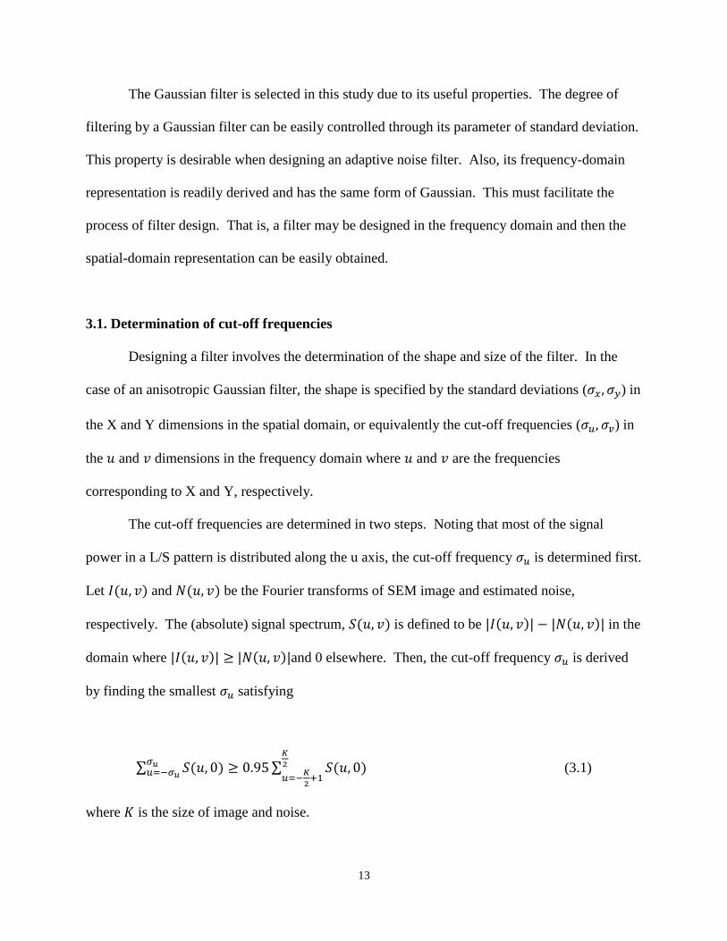
3.1. Determination of cut-off frequencies

Designing a filter involves the determination of the shape and size of the filter. In the

case of an anisotropic Gaussian filter, the shape is specified by the standard deviations (𝜎𝑥, 𝜎𝑦) in

the X and Y dimensions in the spatial domain, or equivalently the cut-off frequencies (𝜎𝑢, 𝜎𝑣) in

the 𝑢 and 𝑣 dimensions in the frequency domain where 𝑢 and 𝑣 are the frequencies

corresponding to X and Y, respectively.

The cut-off frequencies are determined in two steps. Noting that most of the signal

power in a L/S pattern is distributed along the u axis, the cut-off frequency 𝜎𝑢 is determined first.

Let 𝐼(𝑢, 𝑣) and 𝑁(𝑢, 𝑣) be the Fourier transforms of SEM image and estimated noise,

respectively. The (absolute) signal spectrum, 𝑆(𝑢, 𝑣) is defined to be |𝐼(𝑢, 𝑣)| − |𝑁(𝑢, 𝑣)| in the

domain where |𝐼(𝑢, 𝑣)| ≥ |𝑁(𝑢, 𝑣)|and 0 elsewhere. Then, the cut-off frequency 𝜎𝑢 is derived

by finding the smallest 𝜎𝑢 satisfying

∑ 𝑆(𝑢, 0) ≥ 0.95𝜎𝑢𝑢=−𝜎𝑢

∑ 𝑆(𝑢, 0)𝐾

2

𝑢=−𝐾

2+1

(3.1)

where 𝐾 is the size of image and noise.

14

That is, the cut-off frequency 𝜎𝑢 is set such that 95% of the signal power on the 𝑢 axis is

included. The noise is not explicitly considered in the determination of 𝜎𝑢 in this step. The cut-

off frequency 𝜎𝑣 is determined in the similar way as in the previous study, but with 𝜎𝑢 fixed. Let

𝐺(𝑢, 𝑣: 𝜎𝑢) denote the Gaussian filter in the frequency domain, in which the standard deviation

of a Gaussian filter along the 𝑢 dimension is set to 𝜎𝑢. Using 𝐺(𝑢, 𝑣: 𝜎𝑢), the standard deviation

along the 𝑣 dimension is found such that the signal power is not less than the noise power after

the filtering, i.e., the maximum frequency of 𝑣 for which the ratio defined below is not less than

1 [7]. Then, the 𝜎𝑣 is set to the maximum frequency (see equation 3.2).

∑ ∑ |𝐼(𝑢,𝑣)|𝐺(𝑢,𝑣:𝜎𝑢)−∑ ∑ |𝑁(𝑢,𝑣)|𝐺(𝑢,𝑣:𝜎𝑢)𝐾−1

𝑢=0𝐾−1𝑣=0

𝐾−1𝑢=0

𝐾−1𝑣=0

∑ ∑ |𝑁(𝑢,𝑣)|𝐺(𝑢,𝑣:𝜎𝑢)𝐾−1𝑢=0

𝐾−1𝑣=0

(3.2)

The idea is to determine the 𝜎𝑢 by including most of the frequency components of line

features in a L/S pattern and then the 𝜎𝑣 by allowing the smoothing until the noise does not

become dominant. That is, the 𝜎𝑢 is determined mainly by the features while the 𝜎𝑣 is

influenced more by the noise. In Fig. 3.2, a filtered SEM image is compared with the SEM image

before the filtering.

Figure 3.2: An example of magnified SEM image: (a) after and (b) before filtering

15

3.2. Boundary detection

After the noise filtering, the detection of feature boundaries is carried out using an edge

detector. As in the previous study [7], the Sobel operator is employed. Since line features are

assumed to be oriented vertically, the vertical Sobel operator shown below is applied to the filter

SEM image. Then, the pixels with the maximum and minimum gradients within the edge region

are identified to be boundary or edge pixels. In Fig. 3.3, a result of boundary detection is shown.

Figure 3.3: The detected edges are overlaid with the corresponding SEM image.

16

Chapter 4

Results and Discussion

The performance of the anisotropic Gaussian designed by the proposed method has been

analyzed through an extensive simulation.

4.1. Reference images

A set of “reference images” for which the CD and LER are known is generated from real

SEM images (see Fig. 4.1). The boundaries of line features in each SEM image are detected and

taken as real boundaries from which a 3-level (line, space and edge regions) region-wise uniform

image is created. By smoothing the region-wise-uniform image in the direction normal to line

features and adding a certain level of noise, a reference image is generated.

Figure 4.1: An example of the reference SEM image.

17

The added noise is made so that it can have no spatial correlation or a spatial correlation

in one or both of horizontal and vertical directions. The actual CD (the width of line in an L/S

pattern) in the transferred pattern may be different from the target CD depending on the dose

used in the pattern transfer and also due to the proximity effect. Since the reference images are

generated from the SEM images of transferred patterns, the line-width in a reference image can

be different from the target line-width. The three target line-widths considered in this study are

50 nm, 60 nm and 120 nm. The CD’s and LER’s in the reference images are listed in Table 4.1.

Size 120nm 60nm

50nm Dose 1.082 Dose 1.000 Dose 0.920 Dose 0.845

LER 4.02 2.24 2.23 2.48 2.39 2.99

CD 121.92 81.35 78.04 75.12 71.67 51.00

Table. 4.1: The known LER and CD in the six reference images.

Each reference image is filtered by the Gaussian filter designed by the proposed design

method. The feature (line) boundaries are detected using the Sobel operator from the filter

reference image. Then, the CD and LER estimated (computed) from the detected feature

boundaries are compared to the known CD and LER, to quantify the CD and LER errors. In

each case, the errors are averaged over 10 simulations. Since the CD error is much smaller than

the LER error and is less than 1% in all cases, the discussion will be mainly focused on the LER

error.

4-2. Comparison with the previous results

The results achieved by the new design method developed in this study are compared

with those by the previous design method. Since the isotropic filter of the previous study did not

18

perform well for the small features, the comparison is made for the line width of 60 nm only. In

Table 4.2, the CD and LER errors for the previous and new design methods are provided. It is

clear that the anisotropic Gaussian filter designed by the new design method performs

significantly better than the isotropic Gaussian filter from the previous study.

Dose

level

Noise level (%) 3.61 9.11 14.59 20.05

Filter type Old

isotropic

Aniso-

tropic

Old

isotropic

Aniso-

tropic

Old

isotropic

Aniso-

tropic

Old

isotropic

Aniso-

tropic

1.082 LER error (%) -13.655 -4.927 -14.781 -1.810 -15.154 -1.105 -14.711 -3.920

CD error (%) -0.686 -0.266 -1.030 -0.280 -1.696 -0.347 -2.692 -0.365

1.000 LER error (%) -16.833 -4.934 -18.376 0.478 -20.315 -1.890 -20.579 -1.104

CD error (%) -0.297 -0.143 -0.535 -0.127 -1.019 -0.120 -1.761 -0.138

0.920 LER error (%) -11.407 -6.670 -14.009 -5.776 -18.522 -3.179 -21.169 -4.527

CD error (%) -0.167 -0.184 -0.169 -0.158 -0.365 -0.149 -0.807 -0.155

0.845 LER error (%) -7.435 -2.285 -8.210 -0.634 -11.606 4.099 -15.738 5.614

CD error (%) -0.258 -0.259 -0.217 -0.219 -0.307 -0.209 -0.747 -0.244

Table. 4.2: Comparison between the isotropic filter designed by the previous method and the

anisotropic filter designed by the new method for the reference images with the target line-width

of 60nm, and horizontally and vertically correlated noise.

In the remaining part of this chapter, the “isotropic filter” refers to an isotropic filter

designed by the new design method. That is, the main focus of discussion will be on the

comparison between an isotropic filter and an anisotropic filter (not between the previous and

current results).

19

4.3. The same type of noise as in SEM images

The results for a set of reference images, where the noise with the same spatial

correlation as in the (real) SEM images is included, are provided in Tables 4.3-4.5. The noise in

the SEM images has a stronger spatial correlation in the horizontal direction than in the vertical

direction, i.e., anisotropic. It can be seen that the CD and LER errors for the anisotropic

(Gaussian) filter are smaller than those for the isotropic filter. The improvement achieved by the

anisotropic filter tends to be larger for a higher level of noise. This may be understood by noting

that the spatial correlation of noise can have a larger effect on the noise filtering when the noise

level is higher. Another observation that can be made is that the 𝜎𝑥 of anisotropic filter does not

vary (increase) as much as the 𝜎𝑦with the noise level. In the proposed method of filter design,

the noise level affects the 𝜎𝑣 more than the 𝜎𝑢 (refer to Section 3).

One exception is that the anisotropic filter leads to larger CD and LER errors compared

to the isotropic filter in the case of the reference image obtained from the SEM image of the L/S

pattern transferred with the normalized dose of 0.920. This reference image includes more-

rapidly-varying feature boundaries. Such boundaries are likely to be smoothed more by the

anisotropic filter in the horizontal direction (refer to 𝜎𝑥), leading to an under-estimation of LER.

Noise level (%) 3.61 9.11 14.59 20.05

Filter type Isotropic Anisotropic Isotropic Anisotropic Isotropic Anisotropic Isotropic Anisotropic

𝜎𝑥 × 𝜎𝑦 (pixel) 1.06×1.06 3.54×0.38 2.18×2.18 3.59×1.59 3.37×3.37 3.16×3.56 4.67×4.67 3.19× 6.15

𝑊𝑥 × 𝑊𝑦 (pixel) 3 × 3 13× 1 7×7 11×5 10×10 10×11 14×14 10×18

LER error (%) 1.424 -1.074 1.275 -0.640 -0.756 -1.167 -4.324 -4.732

CD error (%) -0.132 -0.047 -0.147 -0.059 0.049 0.029 0.053 -0.037

Table. 4.3: Comparison between the isotropic and anisotropic filters designed by the new method for the

reference images with the target line-width of 120nm, and horizontally and vertically correlated noise.

20

Normalized

dose

Noise level (%) 3.61 9.11 14.59 20.05


1.082

𝜎𝑥 × 𝜎𝑦 (pixel) 1.02×1.02 2.71×0.42 2.16×2.16 2.94×1.74 3.37×3.37 3.16×3.56 4.67×4.67 3.19× 6.15

𝑊𝑥 × 𝑊𝑦 (pixel) 3×3 8×1 6 ×6 9 ×5 10×10 10×11 14×14 10×19

LER error (%) 5.000 -4.927 5.140 -1.810 -2.257 -1.105 -9.202 -3.920

CD error (%) -0.027 -0.266 -0.195 -0.280 -0.394 -0.347 -0.906 -0.365

1.000

𝜎𝑥 , 𝜎𝑦 (pixel) 1.01×1.01 2.72×0.36 2.13×2.13 2.73×1.75 3.25×3.25 3.02×3.45 4.37×4.37 3.03×5.99

𝑊𝑥 × 𝑊𝑦 (pixel) 3× 3 8 ×3 6 ×6 8 ×5 10×10 10×11 13×13 10×18

LER error (%) 5.027 -4.934 6.517 0.478 -1.090 -1.890 -7.005 -1.104

CD error (%) 0.034 -0.143 -0.130 -0.127 -0.133 -0.120 -0.367 -0.138

0.920

𝜎𝑥 , 𝜎𝑦 (pixel) 0.92×0.92 2.96×0.32 1.98×1.98 3.4×1.30 2.96× 2.96 3.54×2.57 4.00×4.00 3.69× 4.38

𝑊𝑥 × 𝑊𝑦 (pixel) 3×3 9×1 6× 6 10× 4 9 ×9 11×8 12×12 11×13

LER error (%) 3.722 -6.670 5.670 -5.776 -1.289 3.179 5.660 -4.527

CD error (%) -0.042 -0.184 -0.183 -0.158 -0.141 -0.149 -0.180 -0.155

0.845

𝜎𝑥 , 𝜎𝑦 (pixel) 0.97×0.97 3.38×0.32 1.92×1.92 3.39×1.14 2.87×2.87 3.45×2.41 3.79×3.79 3.50× 4.12

𝑊𝑥 × 𝑊𝑦 (pixel) 3×3 10×1 6× 6 10×7 9×9 11×7 12 × 12 11×12

LER error (%) 6.215 -4.556 12.201 -0.634 9.348 4.099 4.246 5.614

CD error (%) -0.125 -0.259 -0.305 -0.219 -0.232 -0.209 -0.241 -0.244

Table. 4.4: Comparison between the isotropic and anisotropic filters designed by the new method

for the reference images with the target line-width of 60nm, and horizontally and vertically

correlated noise.

Noise level (%) 3.61 9.11 14.59 20.05


𝜎𝑥 × 𝜎𝑦 (pixel) 0.91×0.91 3.26×0.32 1.60×1.60 3.23×0.77 2.17×2.17 3.18×1.45 2.66×2.66 3.18×2.21

𝑊𝑥 × 𝑊𝑦 (pixel) 3×3 10×1 5×5 10×2 7 ×7 10×5 8×8 10×7

LER error (%) 3.338 -2.327 7.770 -0.798 10.113 2.734 11.452 7.339

CD error (%) 0.061 -0.192 -0.079 -0.238 -0.119 -0.238 -0.180 -0.287


for the reference images with the target line-width of 50nm, and horizontally and vertically

correlated noise.

21

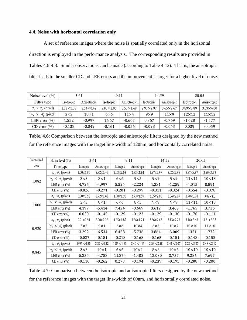
4.4. Noise with horizontal correlation only

A set of reference images where the noise is spatially correlated only in the horizontal

direction is employed in the performance analysis. The corresponding results are provided in

Tables 4.6-4.8. Similar observations can be made (according to Table 4-12). That is, the anisotropic

filter leads to the smaller CD and LER errors and the improvement is larger for a higher level of noise.

Noise level (%) 3.61 9.11 14.59 20.05


𝜎𝑥 × 𝜎𝑦 (pixel) 1.03×1.03 3.54×0.42 2.05×2.05 3.57×1.49 2.97×2.97 3.65×2.67 3.89×3.89 3.69×4.00

𝑊𝑥 × 𝑊𝑦 (pixel) 3×3 10×1 6×6 11×4 9×9 11×9 12×12 11×12

LER error (%) 1.552 -0.997 1.867 -0.667 0.367 -0.769 -1.628 -1.577

CD error (%) -0.138 -0.049 -0.161 -0.056 -0.098 -0.043 0.039 -0.059


for the reference images with the target line-width of 120nm, and horizontally correlated noise.

Normalized

dose

Noise level (%) 3.61 9.11 14.59 20.05


1.082

𝜎𝑥 , 𝜎𝑦 (pixel) 1.00×1.00 2.72×0.46 2.03×2.03 2.83×1.64 2.97×2.97 3.02×2.95 3.87×3.87 3.20×4.39

𝑊𝑥 × 𝑊𝑦 (pixel) 3×3 8×1 6×6 9×5 9×9 9×9 11×11 10×13

LER error (%) 4.725 -4.997 5.524 -2.224 1.331 -1.259 -4.015 0.891

CD error (%) -0.026 -0.271 -0.201 -0.299 -0.311 -0.324 -0.554 -0.378

1.000

𝜎𝑥 , 𝜎𝑦 (pixel) 0.98×0.98 2.72×0.40 1.98×1.98 2.73×1.59 2.85×2.85 2.84×2.87 3.70×3.70 3.02×4.3

𝑊𝑥 × 𝑊𝑦 (pixel) 3×3 8×1 6×6 8×5 9×9 9×9 11×11 10×13

LER error (%) 4.197 -5.414 7.424 -0.669 3.612 3.463 -1.765 3.726

CD error (%) 0.030 -0.145 -0.129 -0.123 -0.129 -0.130 -0.170 -0.111

0.920

𝜎𝑥 , 𝜎𝑦 (pixel) 0.91×0.91 2.90×0.32 1.85×1.85 3.26×1.24 2.66×2.66 3.43×2.23 3.46×3.46 3.61×3.37

𝑊𝑥 × 𝑊𝑦 (pixel) 3×3 9×1 6×6 10×4 8×8 10×7 10×10 11×10

LER error (%) 3.292 -6.534 6.458 -5.736 3.864 -3.009 1.351 1.772

CD error (%) -0.037 -0.181 -0.218 -0.168 -0.165 -0.151 -0.148 -0.153

0.845

𝜎𝑥 , 𝜎𝑦 (pixel) 0.95×0.95 3.37×0.32 1.85×1.85 3.40×1.15 2.58×2.58 3.41×2.07 3.27×3.27 3.43×3.17

𝑊𝑥 × 𝑊𝑦 (pixel) 3×3 10×1 6×6 10×4 8×8 10×6 10×10 10×10

LER error (%) 5.354 -4.788 11.374 -1.403 12.030 3.757 9.286 7.697

CD error (%) -0.110 -0.262 0.273 -0.194 -0.239 -0.195 -0.208 -0.200



22

Noise level (%) 3.61 9.11 14.59 20.05


𝜎𝑥 × 𝜎𝑦 (pixel) 0.92×0.92 3.26×0.32 1.53×1.53 3.20× 0.71 2.01×2.01 3.23×1.27 2.47×2.47 3.19×1.97

𝑊𝑥 × 𝑊𝑦 (pixel) 3×3 10×3 5×5 10×2 6×6 10×7 8×8 10×7

LER error (%) 2.876 -2.418 7.979 -0.984 10.707 1.957 12.047 6.157

CD error (%) 0.077 -0.183 -0.124 -0.257 -0.134 -0.293 -0.190 -0.324



4.5. Noise with no spatial correlation

The results for the reference images with the spatially-uncorrelated noise are provided in

Tables 4.9-11. It is noticed that the improvement by the anisotropic filter is relatively larger

compared to the cases where the noise is spatially correlated. The spatially-uncorrelated noise is

easier to filter in general. And the 𝜎𝑥 is set mainly to include the feature frequency components

sufficiently and the 𝜎𝑦 is determined mostly by the degree of noise filtering needed. Therefore,

for a reference image with a spatially-uncorrelated noise, the 𝜎𝑦 needs to be smaller while the 𝜎𝑥

is similar with that for the case of a spatially-correlated noise. Hence, the difference between the

𝜎𝑥 and 𝜎𝑦 is to be larger (refer to Table 4.13). However, an isotropic filter has no such

adaptability since 𝜎𝑥 must be the same as the 𝜎𝑦.

Noise level (%) 3.61 9.11 14.59 20.05


𝜎𝑥 × 𝜎𝑦 (pixel) 0.84×0.84 3.54×0.32 1.43×1.43 3.54×0.66 1.91×1.91 3.62×1.19 2.35×2.35 3.67×1.67

𝑊𝑥 × 𝑊𝑦 (pixel) 3×3 11×1 4×4 11×2 6×6 11×4 7×7 11×5

LER error (%) 1.709 -0.859 3.172 -0.979 3.477 -0.724 3.526 -0.376

CD error (%) -0.137 -0.035 -0.163 -0.054 -0.120 -0.045 -0.142 -0.045


for the reference images with the target line-width of 120nm, and noise with no spatial correlation.

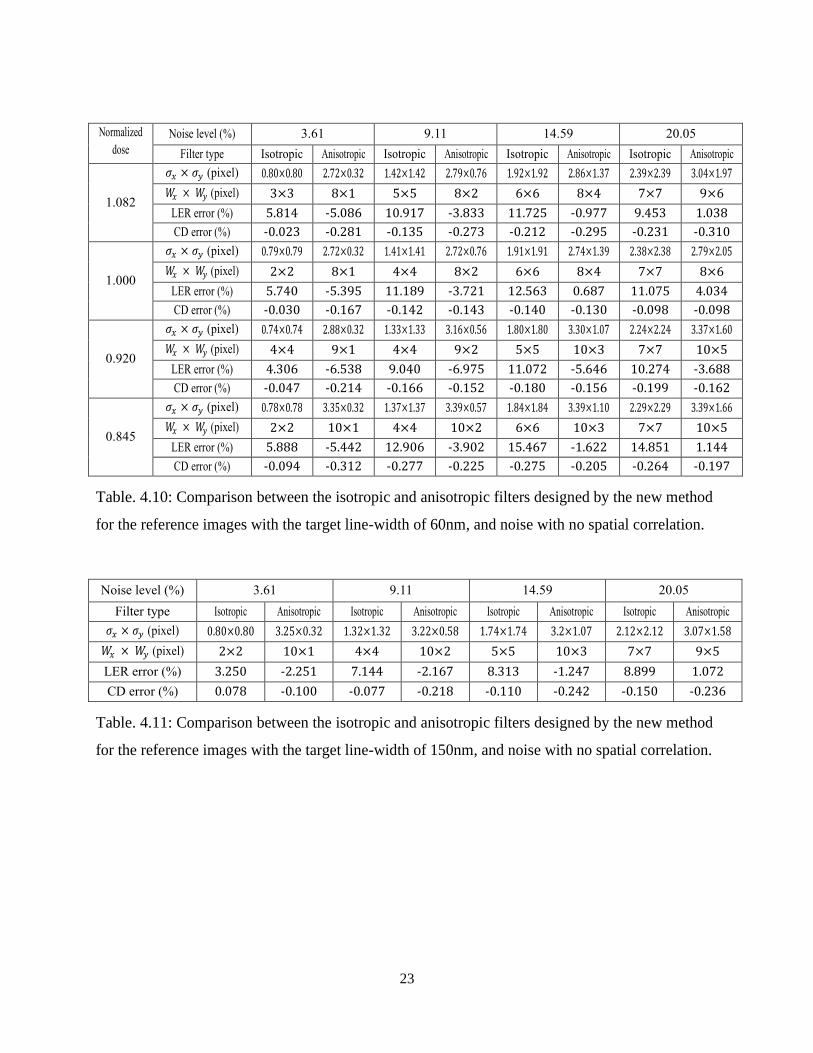
23

Normalized

dose

Noise level (%) 3.61 9.11 14.59 20.05


1.082

𝜎𝑥 × 𝜎𝑦 (pixel) 0.80×0.80 2.72×0.32 1.42×1.42 2.79×0.76 1.92×1.92 2.86×1.37 2.39×2.39 3.04×1.97

𝑊𝑥 × 𝑊𝑦 (pixel) 3×3 8×1 5×5 8×2 6×6 8×4 7×7 9×6

LER error (%) 5.814 -5.086 10.917 -3.833 11.725 -0.977 9.453 1.038

CD error (%) -0.023 -0.281 -0.135 -0.273 -0.212 -0.295 -0.231 -0.310

1.000

𝜎𝑥 × 𝜎𝑦 (pixel) 0.79×0.79 2.72×0.32 1.41×1.41 2.72×0.76 1.91×1.91 2.74×1.39 2.38×2.38 2.79×2.05

𝑊𝑥 × 𝑊𝑦 (pixel) 2×2 8×1 4×4 8×2 6×6 8×4 7×7 8×6

LER error (%) 5.740 -5.395 11.189 -3.721 12.563 0.687 11.075 4.034

CD error (%) -0.030 -0.167 -0.142 -0.143 -0.140 -0.130 -0.098 -0.098

0.920

𝜎𝑥 × 𝜎𝑦 (pixel) 0.74×0.74 2.88×0.32 1.33×1.33 3.16×0.56 1.80×1.80 3.30×1.07 2.24×2.24 3.37×1.60

𝑊𝑥 × 𝑊𝑦 (pixel) 4×4 9×1 4×4 9×2 5×5 10×3 7×7 10×5

LER error (%) 4.306 -6.538 9.040 -6.975 11.072 -5.646 10.274 -3.688

CD error (%) -0.047 -0.214 -0.166 -0.152 -0.180 -0.156 -0.199 -0.162

0.845

𝜎𝑥 × 𝜎𝑦 (pixel) 0.78×0.78 3.35×0.32 1.37×1.37 3.39×0.57 1.84×1.84 3.39×1.10 2.29×2.29 3.39×1.66

𝑊𝑥 × 𝑊𝑦 (pixel) 2×2 10×1 4×4 10×2 6×6 10×3 7×7 10×5

LER error (%) 5.888 -5.442 12.906 -3.902 15.467 -1.622 14.851 1.144

CD error (%) -0.094 -0.312 -0.277 -0.225 -0.275 -0.205 -0.264 -0.197



Noise level (%) 3.61 9.11 14.59 20.05


𝜎𝑥 × 𝜎𝑦 (pixel) 0.80×0.80 3.25×0.32 1.32×1.32 3.22×0.58 1.74×1.74 3.2×1.07 2.12×2.12 3.07×1.58

𝑊𝑥 × 𝑊𝑦 (pixel) 2×2 10×1 4×4 10×2 5×5 10×3 7×7 9×5

LER error (%) 3.250 -2.251 7.144 -2.167 8.313 -1.247 8.899 1.072

CD error (%) 0.078 -0.100 -0.077 -0.218 -0.110 -0.242 -0.150 -0.236



24

4.6. Feature size

The CD and LER errors are averaged for each feature size in each case of noise type in

Table 4.12-13. It is clear that the performance of anisotropic filter is better in all cases and more

consistent independent of the feature size and noise type. The isotropic filter leads to a

significantly larger average LER error for smaller features (50 nm, 60 nm) than for a larger

feature (120 nm). On the other hand, the average LER error achieved by the anisotropic filter

shows only a small variation with the feature size and noise type. This is most likely due to the

better adaptability of an anisotropic filter.

Size

(nm)

The same type of noise as in SEM

images

Noise with horizontal correlation

only Noise with no spatial correlation

Isotropic Anisotropic Isotropic Anisotropic Isotropic Anisotropic

CD

error

(%)

LER

error

(%)

CD

error

(%)

LER

error

(%)

CD

error

(%)

LER

error

(%)

CD

error

(%)

LER

error

(%)

CD

error

(%)

LER

error

(%)

CD

error

(%)

LER

error

(%)

120 0.095 1.945 0.043 1.903 0.109 1.354 0.052 1.002 0.141 2.971 0.045 0.735

60 0.227 5.599 0.21 3.451 0.184 5.35 0.205 3.584 0.157 10.142 0.207 3.733

50 0.11 8.168 0.239 3.3 0.131 8.402 0.264 2.879 0.104 6.902 0.199 1.684

Table. 4.12: The average CD and LER errors for each target line-width.

Size

(nm)

The same type of noise as in SEM

images

Noise with horizontal correlation

only Noise with no spatial correlation

Isotropic Anisotropic Isotropic Anisotropic Isotropic Anisotropic

σx 𝜎𝑦 σx 𝜎𝑦 σx 𝜎𝑦 σx 𝜎𝑦 σx 𝜎𝑦 σx 𝜎𝑦

120 2.831 2.831 3.667 2.609 2.485 2.485 3.611 2.146 1.634 1.634 3.583 0.953

60 2.588 2.588 3.176 2.500 2.307 2.307 3.118 2.027 1.587 1.587 3.039 1.008

50 1.837 1.837 3.215 1.191 1.731 1.731 3.226 1.065 1.494 1.494 3.186 0.888

Table. 4.13: The average filter size for each target line-width.

25

Chapter 5

Conclusion

In this study, the issue of designing a noise filter to be used in the analysis of SEM

images for detecting feature boundaries has been addressed with L/S patterns. An ultimate goal

of the analysis is to measure the CD and LER of features from the detected feature boundaries.

The specific motivation is to improve the performance of a previously-designed filter which is

not able to achieve as high accuracy for relatively small features as for large features. The

previous design method requires the same cut-off frequency in both horizontal and vertical

dimensions, which leads to an isotropic filter. The new design method developed in this study

allows the two cut-off frequencies to be different. The resulted filter becomes anisotropic and

has a better adaptability to the noise type and level. The cut-off frequency of the filter in the

direction normal to line features is first determined such that a sufficient amount of feature

frequency components is included. Then, the cut-off frequency in the other direction is

determined according to the degree of noise filtering needed. Also, compared to the previous

method, the procedure of noise estimation has been improved in the determination of the width

of flat region to be extracted (and the DC level to be removed). Through an extensive simulation

study, it has been shown that the anisotropic Gaussian filter designed by the new design method

can perform better in enabling the accurate measurement of CD and LER. The CD and LER

errors by the anisotropic filter are significantly smaller than those by the isotropic filter. The

anisotropic filter is more adaptive to the noise type and level and its performance is less sensitive

26

to the feature size and noise type. Therefore, the new design method can be considered to

have a potential to be employed in real applications.

It is worthwhile to point out that this design method relies on the noise estimated from a

given SEM image. As the feature size (line width) decreases, the width of flat region from

which the noise is estimated decreases, making the estimated noise less accurate. A further

refinement of the noise estimation procedure may be needed.

27

Reference

[1] A. A. Tseng, K. Chen, C. D. Chen, and K. J. Ma, “Electron Beam Lithography in Nanoscale

Fabrication: Recent Development”, IEEE. Trans. Electron. Packag. Manuf. 26, 141 (2003).

[2] R. Murali, D. Brown, K. Martin, and J. Meindl, “Process optimization and proximity effect

correction for gray scale e-beam lithography”, J. Vac. Sci. Technol., B 24, 2936 (2006).

[3] M. J. Burek and J. R. Greer, “Fabrication and Microstructure Control of Nanoscale

Mechanical Testing Specimens via Electron Beam Lithography and Electroplating”, Nano. Lett.

10, 69 (2010).

[4] Q. Dai, S.-Y. Lee, S.-H. Lee, B.-G. Kim, and H.-K. Cho, “Estimation of resist profile for

line/space patterns using layer-based exposure modeling in electron-beam lithography”,

Microelectron. Eng. 88, 902 (2011).

[5] W. Chen and H. Ahmed, “Fabrication of 5–7 nm wide etched lines in silicon using 100 keV

e‐beam lithography and polymethylmethacrylate resist”, Appl. Phys. Lett. 62, 1499 (1993).

[6] R. Guo, S.-Y. Lee, J. Choi, S.-H. Park, I.-K. Shin, and C.-U. Jeon, “Practical approach to

modeling e-beam lithographic process from SEM images for minimization of line edge

roughness and critical dimension error”, J. Vac. Sci. Technol., B 34, 011601 (2016).

[7] D. Li, R. Guo, S.-Y. Lee, J. Choi, S.-H. Park, S.-B. Kim, I.-K. Shin, and C.-U. Jeon, “Noise

filtering for accurate measurement of line edge roughness and critical dimension”, J. Vac. Sci.

and Technol., B 34(6), 60K604, Nov/Dec 2016.

[8] G. P. Patsis et al., “Quantification of line-edge roughness of photoresists. I. A comparison

between off-line and on-line analysis of topdown scanning electron microscopy images”, J. Vac.

Sci. Technol. B: Microelectron. Nanometer Struct. 21(3), 1008–1018 (2003).

[9] T. Verduin, P. Kruit, and C. W. Hagen, “Determination of line edge roughness in low-dose

top-down scanning electron microscopy images”, J. Micro/Nanolithogr. MEMS MOEMS 13,

033009 (2014).

http://www.eng.auburn.edu/~sylee/pyramid_papers/JVST_FilterDesign.pdf



28

[10] A. Yamaguchi and J. Yamamoto, “Influence of image processing on line-edge roughness in

CD-SEM measurement”, Proc. SPIE 6922, 692221 (2008).

[11] A. Hiraiwa and A. Nishida, “Statistically accurate analysis of line width roughness based on

discrete power spectrum”, Proc. SPIE 7638,76380N (2010).

[12] A. Nishida, “Statistical- and image-noise effects on experimental spectrum of line-edge and

line-width roughness”, J. Micro/Nanolithogr., MEMS, MOEMS 9(4), 041210 (2010).

[13] A. Yamaguchi et al., “Bias-free measurement of LER/LWR with low damage by CD-SEM”,

Proc. SPIE 6152, 61522D (2006).

[14] A. Hiraiwa, “Image-pixel averaging for accurate analysis of line-edge and linewidth

roughness”, J. Micro/Nanolithogr., MEMS, MOEMS 10(2), 023010 (2011).

[15] V. Constantoudis and E. Pargon, “Evaluation of methods for noise-free measurement of

LER/LWR using synthesized CD-SEM images”, Proc. SPIE 8681, 86812L (2013).

[16] T. F. Coleman and Y. Li, “An interior trust region approach for nonlinear minimization

subject to bounds”, SIAM J. Optim. 6(2), 418–445 (1996).

[17] S.-Y. Lee and K. Anbumony, “Accurate control of remaining resist depth for nanoscale

three-dimensional structures in electron-beam grayscale lithography”, Journal of Vacuum

Science and Technology, B 25(6), pp. 2008-2012, Nov. 2007.

[18] S.-Y. Lee and K. Anbumony, “Analysis of three-dimensional proximity effect in electron-

beam lithography”, Microelectronic Engineering, vol. 83(2), pp. 336-344, Feb. 2006.

[19] Q. Dai, R. Guo, S.-Y. Lee, J. Choi, S.-H. Lee, I.-K. Shin, C.-U. Jeon, B.-G. Kim, and H.-K.

Cho, “A fast path-based method for 3-D resist development simulation”, Microelectron. Eng.

127, 86 (2014).

[20] C. A. Mack, “Stochastic modeling of photoresist development in two and three dimensions”,

J. Micro/Nanolith. MEMS MOEMS 9(4), 041202 (2010).

[21] C.Guo, S.-Y. Lee, S. H. Lee, B.-G. Kim, and H.-K. Cho, “Application of neural network to

controlling three-dimensional electron-beam exposure distribution in resist,” J. Vac. Sci.

Technol., B 27, 2572 (2009).

29

[22] P. Kruit and S. Steenbrink, “Shot noise in electron-beam lithography and line-width

measurements”, Scanning 28(1), 20–26 (2006).

[23] Y. H. Lin and D. C. Joy, “A new examination of secondary electron yield data”, Surf.

Interface Anal. 37, 895 (2005).

[24] H. Seiler, J. “Secondary electron emission in the scanning electron microscope”, Appl. Phys.

54, R1 (1983).

[25] S.-Y. Lee and Kasi Anbumony, “Analysis of Three-Dimensional Proximity Effect in

Electron-Beam Lithography”, Microelectron. Eng. 83, 336-344 (2006)

designing an anisotropic noise filter for measuring

Documents