cancellation of white and color noise with adaptive filter...

International Journal of Wireless & Mobile Networks (IJWMN) Vol. 7, No. 4, August 2015

DOI : 10.5121/ijwmn.2015.7402 19

CANCELLATION OF WHITE AND COLOR

NOISE WITH ADAPTIVE FILTER USING LMS

ALGORITHM

1Solaiman Ahmed,

2Farhana Afroz,

1Ahmad Tawsif and

1Asadul Huq

1Department of Electrical and Electronic Engineering,

University of Dhaka, Bangladesh 2Faculty of Engineering and Information Technology,

University of Technology, Sydney, Australia

ABSTRACT

In this paper, the performances of adaptive noise cancelling system employing Least Mean Square (LMS)

algorithm are studied considering both white Gaussian noise (Case 1) and colored noise (Case 2)

situations. Performance is analysed with varying number of iterations, Signal to Noise Ratio (SNR) and tap

size with considering Mean Square Error (MSE) as the performance measurement criteria. Results show

that the noise reduction is better as well as convergence speed is faster for Case 2 as compared with Case

1. It is also observed that MSE decreases with increasing SNR with relatively faster decrease of MSE in

Case 2 as compared with Case 1, and on average MSE increases linearly with increasing number of filter

coefficients for both type of noise situations. All the experiments have been done using computer

simulations implemented on MATLAB platform.

KEYWORDS

Adaptive Noise Canceller, Color Noise, LMS, MSE, Number of Iterations, SNR, Tap Size, White Gaussian

Noise

1.INTRODUCTION

Extracting the speech signal of interest from the noise-corrupted signal is an important signal

processing operation in voice communication systems. A frequently encountered problem in

communication system is the contamination of the useful signals by unwanted signals or noise.

In noise cancellation, signal processing operations involve to filtering out the unwanted noise or

interference from the signal contaminated by noise so that the desired signal can be recovered.

The spectral characteristics of noise is time varying and unknown in many circumstances. In

addition, noise power may exceed the power of the useful signal. In such situations, adaptive

digital filters can show better performance in cancelling background noise as compared with


20

conventional non-adaptive filters. In adaptive noise cancelling system, noise cancellation

becomes an adaptive process i.e. the system gets adjusted itself according to the changing

environment. Adaptive noise cancellation is a process of subduing background noise from the

desired signal in an adaptive manner so as improved SNR (Signal to Noise Ratio) can be ensured

at the receiving end [1, 2]. The use of adaptive digital filter in noise cancelling system is at the

core for achieving this adaptation capability of the system. In adaptive filter, the filter coefficients

can be modified intelligently using adaptive algorithms so that the filter can keep track to the

instantaneous changes being occurred in its input characteristics [3]. A range of adaptive

algorithms has been proposed to achieve optimum system performance in many applications.

Some of the proposed adaptive algorithms can be found in [4-10]. In this paper, a comparative

study of eliminating white Gaussian noise and colored noise employing LMS algorithm will be

reported. Moreover, the convergence curves as well as the effects of number of iterations, SNR

and filter taps on the performance of the system will be evaluated considering both type of noise

situations.

The rest of the paper is organized as follows. Section 2 provides a brief review of noise in

communication system. Adaptive noise cancellation process is explained in Section 3 followed by

illustration of LMS algorithm in Section 4. The simulation parameters and results are discussed in

Section 5. Finally, this paper is concluded with Section 6.

2.NOISE IN COMMUNICATION SYSTEM

Noise is random in nature. It is unwanted form of energy that enters the communication system

and interferes with the information signal. Noise degrades the level of quality of the received

signal at the receiver. Noise can be classified as internal noise and external noise. White noise is a

Gaussian noise which exists in all frequencies, whereas colored noise exists in some bands of

frequencies.

2.1. White Gaussian Noise

The common source of noise which affects communication is usually white noise. The probability

density function of white noise is normal distribution known as Gaussian distribution. Its power

spectral density is flat and occupies all frequency. In signal processing, a random signal is

considered "white noise" if it is observed to have a flat spectrum over the range of frequencies

[11]. Theoretically bandwidth of white noise is infinite. But the bandwidth of this noise is limited

in practice by the mechanism of noise generation.

2.2. Color Noise

The color noise is generally characterized by its power spectral density. The noise of different

color has different impact on signals. Power spectral density per unit of bandwidth is proportional

to 1/fβ. For white noise, β=o, for

pink noise, β=1 and for brown noise, β=2.

In pink noise, the frequency spectrum is logarithmic space and it has equal power in bands that

are proportionally wide. The power decreases by 3 db octave compared with white noise. Pink

noise sounds more natural than white noise. It sounds like rushing water.


21

Brownian noise or Red noise may refer to any system where power spectral density decreases

with increasing frequency. The name is after the corruption of Brownian motion. This is also

known as ‘random walk’ noise [12].

Blue noise’s power spectral density increases 3 db per octave with increasing frequency over a

finite frequency range. There are no concentrated spikes in energy. Retinal cells are arranged in a

blue noise pattern which yields good visual resolution [13].

Violet noise’s power density increases 6 db per octave with increasing frequency over a finite

frequency range. It is also known as differentiated white noise. Acoustic thermal noise of water

has a violet spectrum [14].

Grey noise is random white noise over a certain frequency range .This is a contrast to standard

white noise which has equal strength over a linear scale of frequencies.

3.ADAPTIVE FILTER FOR NOISE CANCELLATION

The principal of adaptive filtering is to obtain an optimum estimate of the noise and subtract it

from the noisy signal. When the speech signal and noise contained in the primary input are

uncorrelated and no crosstalk conditions are met, then adaptive noise cancelling techniques allow

reduction of noise without information signal distortion. An adaptive filter works as the model

that relates the primary input signals and adaptive filter output signal in real time in an iterative

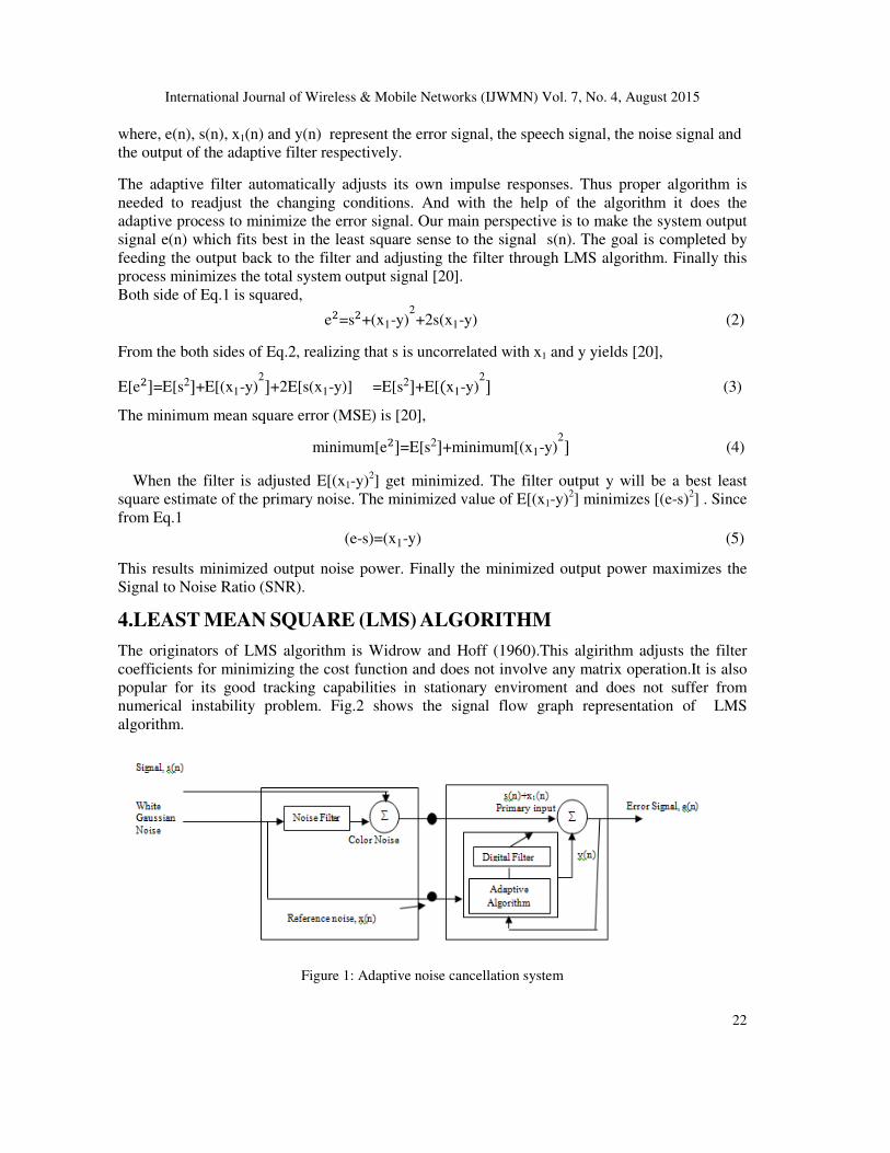
manner [15]. The concept of adaptive filter is shown in Fig. 1. It has a Finite Impulse Response

(FIR) structure. For such structures, the impulse response is equal to the filter coefficients [16]. It

is a nonlinear filter since its characteristics are not independent on the input signal and

consequently the homogeneity conditions are not satisfied. If we freeze the filter parameters at a

given instant of time, most adaptive filters are linear in the sense that their output signals are

linear functions of their input signals [17]

The contaminated signal passes through the filter. The filter suppresses noises from the

contaminated signal and this process does not require priory idea about the signal and noise. In

adaptive noise cancellation, one channel is used as the input path of speech that is corrupted by

the white or color noise and the other input is used as the reference white Gaussian noise. Color

noise can be obtained by passing the white noise through a Chebyshev filter to get an output noise

which is concentrated at the pass band region of the filter. The signal can be corrupted by white,

color or both white and color noise.

The speech signal and noise are expressed as s (n) and x1 (n) respectively. The reference noise is

expressed as x (n) and output of the adaptive filter is denoted as y (n) which is produced as close

as possible of x1(n).The filter readjust itself in the continuous process. This continuous

adjustment process minimizes the error between x1(n) and y (n) [18].

Signal is uncorrelated with noise x1(n). The signal s(n) and noise x1(n) combined to form the

desired signal d(n) = s(n) + x1(n). Reference noise x(n) is uncorrelated with the signal but

correlated in some unknown way with noise x1(n) [19]. The difference of the output y (n) and the

primary input produces the system output.

e(n)=s(n)+x1(n)-y(n) (1)


22

where, e(n), s(n), x1(n) and y(n) represent the error signal, the speech signal, the noise signal and

the output of the adaptive filter respectively.

The adaptive filter automatically adjusts its own impulse responses. Thus proper algorithm is

needed to readjust the changing conditions. And with the help of the algorithm it does the

adaptive process to minimize the error signal. Our main perspective is to make the system output

signal e(n) which fits best in the least square sense to the signal s(n). The goal is completed by

feeding the output back to the filter and adjusting the filter through LMS algorithm. Finally this

process minimizes the total system output signal [20].

Both side of Eq.1 is squared,

e�=s�+(x1-y)2+2s(x1-y) (2)

From the both sides of Eq.2, realizing that s is uncorrelated with x1 and y yields [20],

E[e�]=E[s2]+E[(x1-y)2]+2E[s(x1-y)] =E[s2]+E[(x1-y)

2] (3)

The minimum mean square error (MSE) is [20],

minimum[e�]=E[s2]+minimum[(x1-y)2] (4)

When the filter is adjusted E[(x1-y)2] get minimized. The filter output y will be a best least

square estimate of the primary noise. The minimized value of E[(x1-y)2] minimizes [(e-s)

2] . Since

from Eq.1

(e-s)=(x1-y) (5)

This results minimized output noise power. Finally the minimized output power maximizes the

Signal to Noise Ratio (SNR).

4.LEAST MEAN SQUARE (LMS) ALGORITHM

The originators of LMS algorithm is Widrow and Hoff (1960).This algirithm adjusts the filter

coefficients for minimizing the cost function and does not involve any matrix operation.It is also

popular for its good tracking capabilities in stationary enviroment and does not suffer from

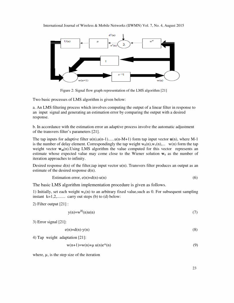
numerical instability problem. Fig.2 shows the signal flow graph representation of LMS

algorithm.

Figure 1: Adaptive noise cancellation system


23

Figure 2: Signal flow graph representation of the LMS algorithm [21]

Two basic processes of LMS algorithm is given below:

a. An LMS filtering process which involves computing the output of a linear filter in response to

an input signal and generating an estimation error by comparing the output with a desired

response.

b. In accordance with the estimation error an adaptive process involve the automatic adjustment

of the transvers filter’s parameters [21].

The tap inputs for adaptive filter u(n),u(n-1)......u(n-M+1) form tap input vector u(n), where M-1

is the number of delay element. Correspondingly the tap weight w0(n),w1(n),... w(n) form the tap

weight vector wm(n).Using LMS algorithm the value computed for this vector represents an

estimate whose expected value may come close to the Wiener solution w0 as the number of

iteration approaches to infinity.

Desired response d(n) of the filter,tap input vector u(n). Transvers filter produces an output as an

estimate of the desired response d(n).

Estimation error, e(n)=d(n)-u(n) (6)

The basic LMS algorithm implementation procedure is given as follows.

1) Initially, set each weight wk(n) to an arbitrary fixed value,such as 0. For subsequent sampling

instant k=1,2,........ carry out steps (b) to (d) below:

2) Filter output [21] : y(n)=wH(n)u(n) (7)

3) Error signal [21]:

e(n)=d(n)-y(n) (8)

4) Tap weight adaptation [21]:

w(n+1)=w(n)+µ u(n)e*(n) (9)

where, µ, is the step size of the iteration


24

5.SIMULATIONS AND RESULTS

In this section, the performance analysis of adaptive noise cancelling system using LMS scheme

will be reported. A comparison of the performances of adaptive noise canceller in case of white

Gaussian noise situation and color noise situation has been made as well as the effect of number

of iterations on the system’s performance is investigated for both case. In addition, the effects of

different parameters such as SNR, tap size on the performance of adaptive noise cancelling

system are studied. The performance is measured in terms of MSE (Mean Square Error). All the

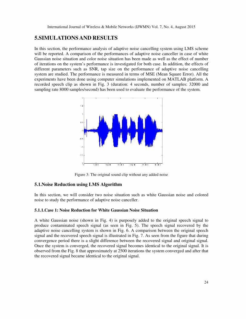
experiments have been done using computer simulations implemented on MATLAB platform. A

recorded speech clip as shown in Fig. 3 (duration: 4 seconds, number of samples: 32000 and

sampling rate 8000 samples/second) has been used to evaluate the performance of the system.

Figure 3: The original sound clip without any added noise

5.1.Noise Reduction using LMS Algorithm

In this section, we will consider two noise situation such as white Gaussian noise and colored

noise to study the performance of adaptive noise canceller.

5.1.1.Case 1: Noise Reduction for White Gaussian Noise Situation

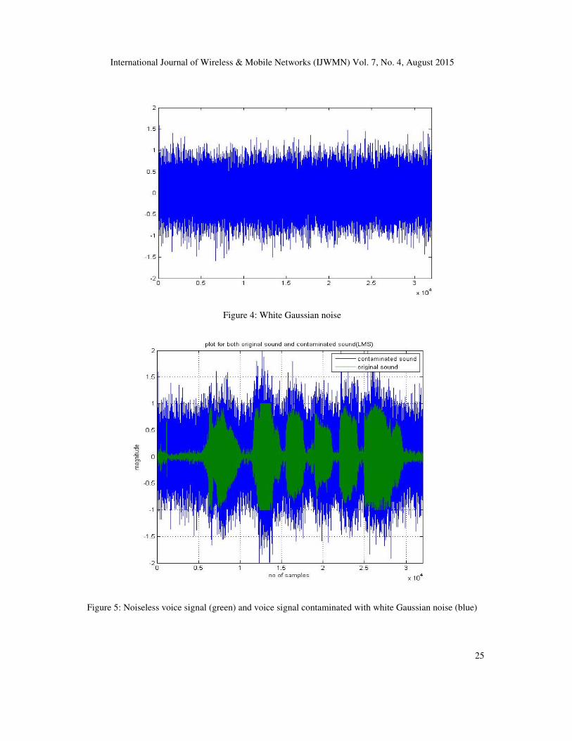
A white Gaussian noise (shown in Fig. 4) is purposely added to the original speech signal to

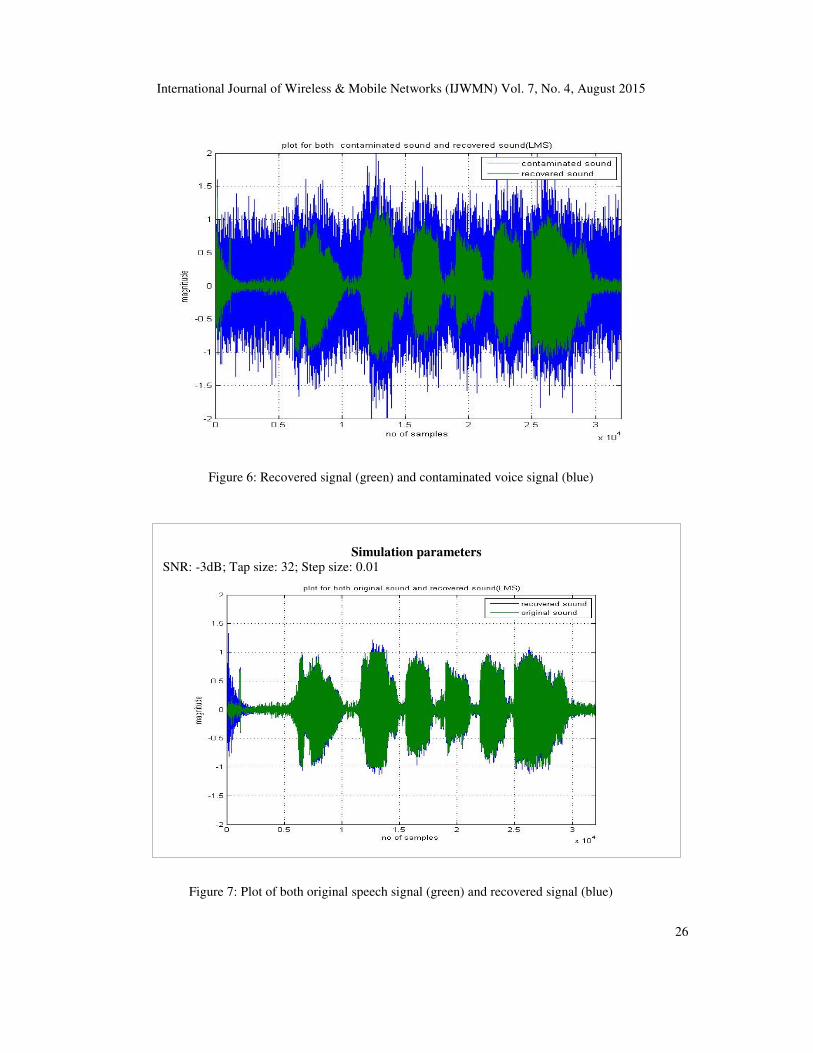
produce contaminated speech signal (as seen in Fig. 5). The speech signal recovered by the

adaptive noise cancelling system is shown in Fig. 6. A comparison between the original speech

signal and the recovered speech signal is illustrated in Fig. 7. As seen from the figure that during

convergence period there is a slight difference between the recovered signal and original signal.

Once the system is converged, the recovered signal becomes identical to the original signal. It is

observed from the Fig. 8 that approximately at 2500 iterations the system converged and after that

the recovered signal became identical to the original signal.


25

Figure 4: White Gaussian noise

Figure 5: Noiseless voice signal (green) and voice signal contaminated with white Gaussian noise (blue)


26

Figure 6: Recovered signal (green) and contaminated voice signal (blue)

Figure 7: Plot of both original speech signal (green) and recovered signal (blue)

Simulation parameters SNR: -3dB; Tap size: 32; Step size: 0.01


27

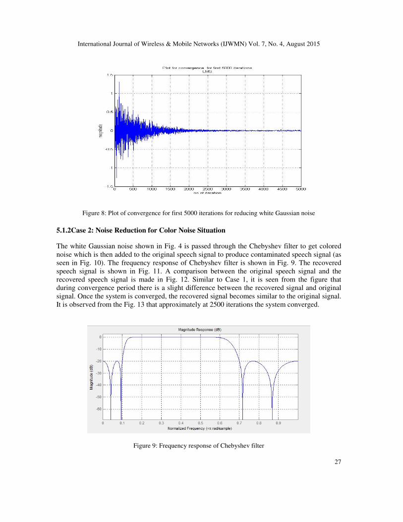
Figure 8: Plot of convergence for first 5000 iterations for reducing white Gaussian noise

5.1.2Case 2: Noise Reduction for Color Noise Situation

The white Gaussian noise shown in Fig. 4 is passed through the Chebyshev filter to get colored

noise which is then added to the original speech signal to produce contaminated speech signal (as

seen in Fig. 10). The frequency response of Chebyshev filter is shown in Fig. 9. The recovered

speech signal is shown in Fig. 11. A comparison between the original speech signal and the

recovered speech signal is made in Fig. 12. Similar to Case 1, it is seen from the figure that

during convergence period there is a slight difference between the recovered signal and original

signal. Once the system is converged, the recovered signal becomes similar to the original signal.

It is observed from the Fig. 13 that approximately at 2500 iterations the system converged.

Figure 9: Frequency response of Chebyshev filter


28

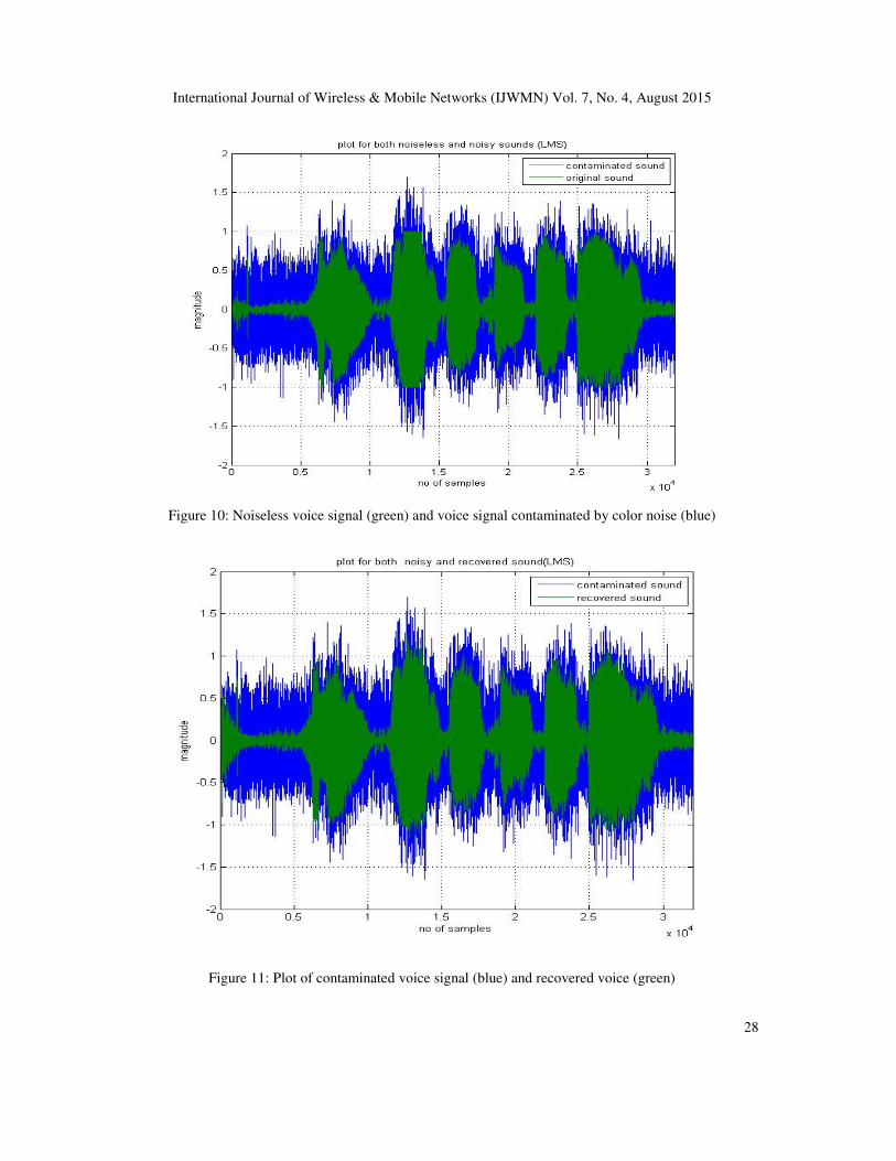
Figure 10: Noiseless voice signal (green) and voice signal contaminated by color noise (blue)

Figure 11: Plot of contaminated voice signal (blue) and recovered voice (green)


29

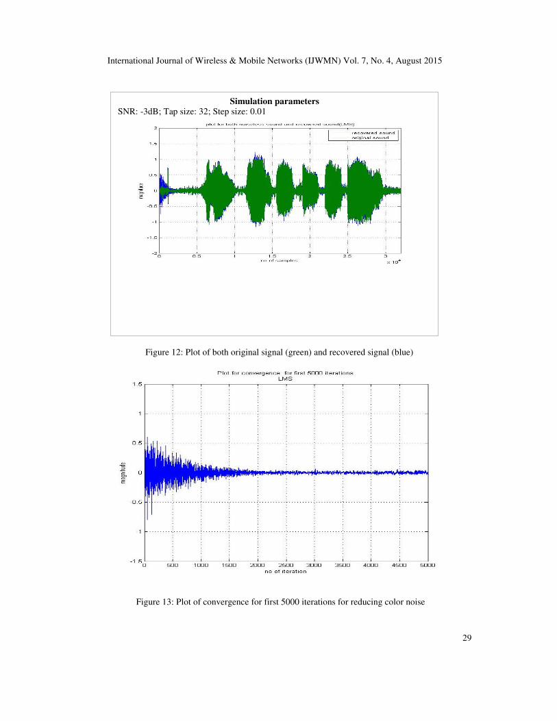
Figure 12: Plot of both original signal (green) and recovered signal (blue)

Figure 13: Plot of convergence for first 5000 iterations for reducing color noise

Simulation parameters SNR: -3dB; Tap size: 32; Step size: 0.01


30

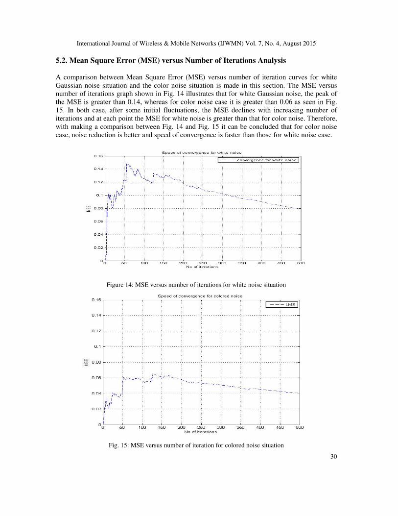
5.2. Mean Square Error (MSE) versus Number of Iterations Analysis

A comparison between Mean Square Error (MSE) versus number of iteration curves for white

Gaussian noise situation and the color noise situation is made in this section. The MSE versus

number of iterations graph shown in Fig. 14 illustrates that for white Gaussian noise, the peak of

the MSE is greater than 0.14, whereas for color noise case it is greater than 0.06 as seen in Fig.

15. In both case, after some initial fluctuations, the MSE declines with increasing number of

iterations and at each point the MSE for white noise is greater than that for color noise. Therefore,

with making a comparison between Fig. 14 and Fig. 15 it can be concluded that for color noise

case, noise reduction is better and speed of convergence is faster than those for white noise case.

Figure 14: MSE versus number of iterations for white noise situation

Fig. 15: MSE versus number of iteration for colored noise situation


31

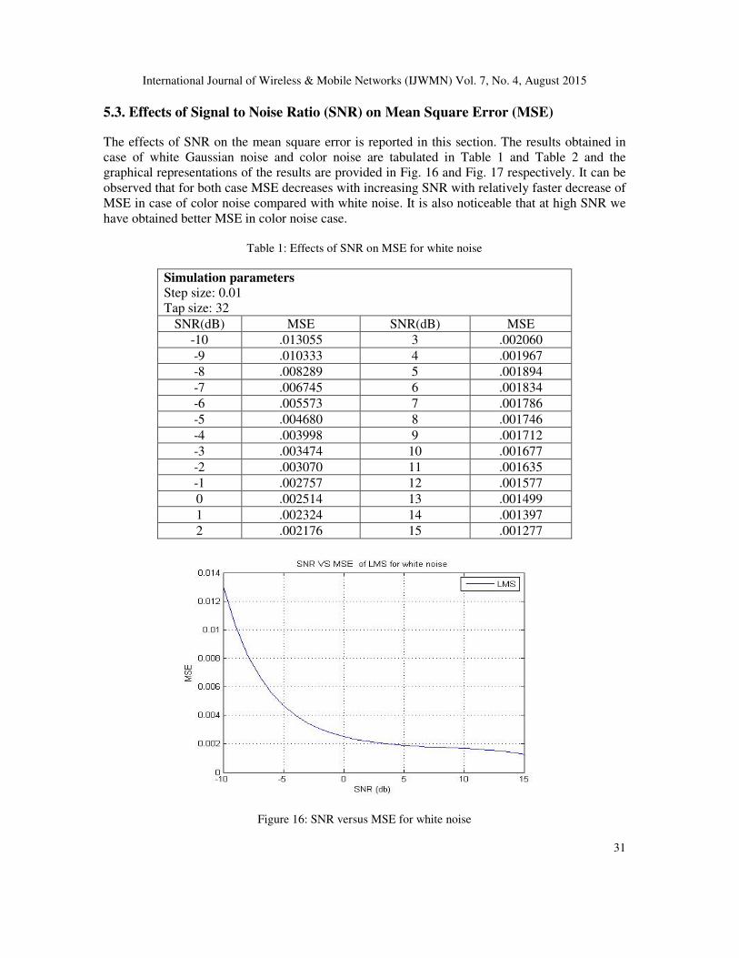
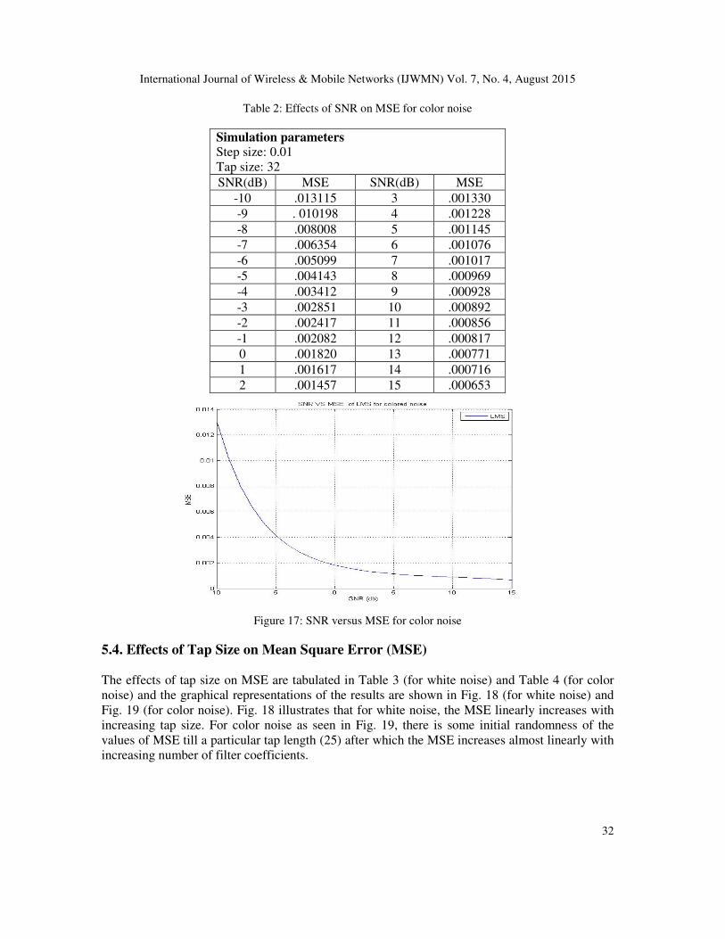
5.3. Effects of Signal to Noise Ratio (SNR) on Mean Square Error (MSE)

The effects of SNR on the mean square error is reported in this section. The results obtained in

case of white Gaussian noise and color noise are tabulated in Table 1 and Table 2 and the

graphical representations of the results are provided in Fig. 16 and Fig. 17 respectively. It can be

observed that for both case MSE decreases with increasing SNR with relatively faster decrease of

MSE in case of color noise compared with white noise. It is also noticeable that at high SNR we

have obtained better MSE in color noise case.

Table 1: Effects of SNR on MSE for white noise

Simulation parameters

Step size: 0.01

Tap size: 32

SNR(dB) MSE SNR(dB) MSE

-10 .013055 3 .002060

-9 .010333 4 .001967

-8 .008289 5 .001894

-7 .006745 6 .001834

-6 .005573 7 .001786

-5 .004680 8 .001746

-4 .003998 9 .001712

-3 .003474 10 .001677

-2 .003070 11 .001635

-1 .002757 12 .001577

0 .002514 13 .001499

1 .002324 14 .001397

2 .002176 15 .001277

Figure 16: SNR versus MSE for white noise


32

Table 2: Effects of SNR on MSE for color noise

Simulation parameters Step size: 0.01

Tap size: 32

SNR(dB) MSE SNR(dB) MSE

-10 .013115 3 .001330

-9 . 010198 4 .001228

-8 .008008 5 .001145

-7 .006354 6 .001076

-6 .005099 7 .001017

-5 .004143 8 .000969

-4 .003412 9 .000928

-3 .002851 10 .000892

-2 .002417 11 .000856

-1 .002082 12 .000817

0 .001820 13 .000771

1 .001617 14 .000716

2 .001457 15 .000653

Figure 17: SNR versus MSE for color noise

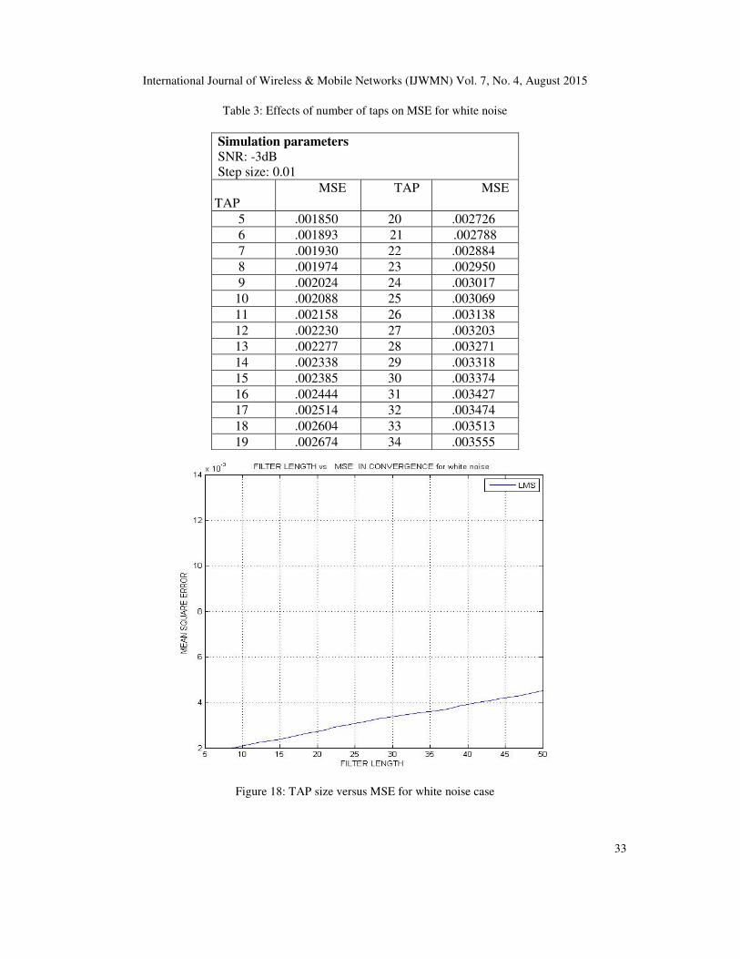
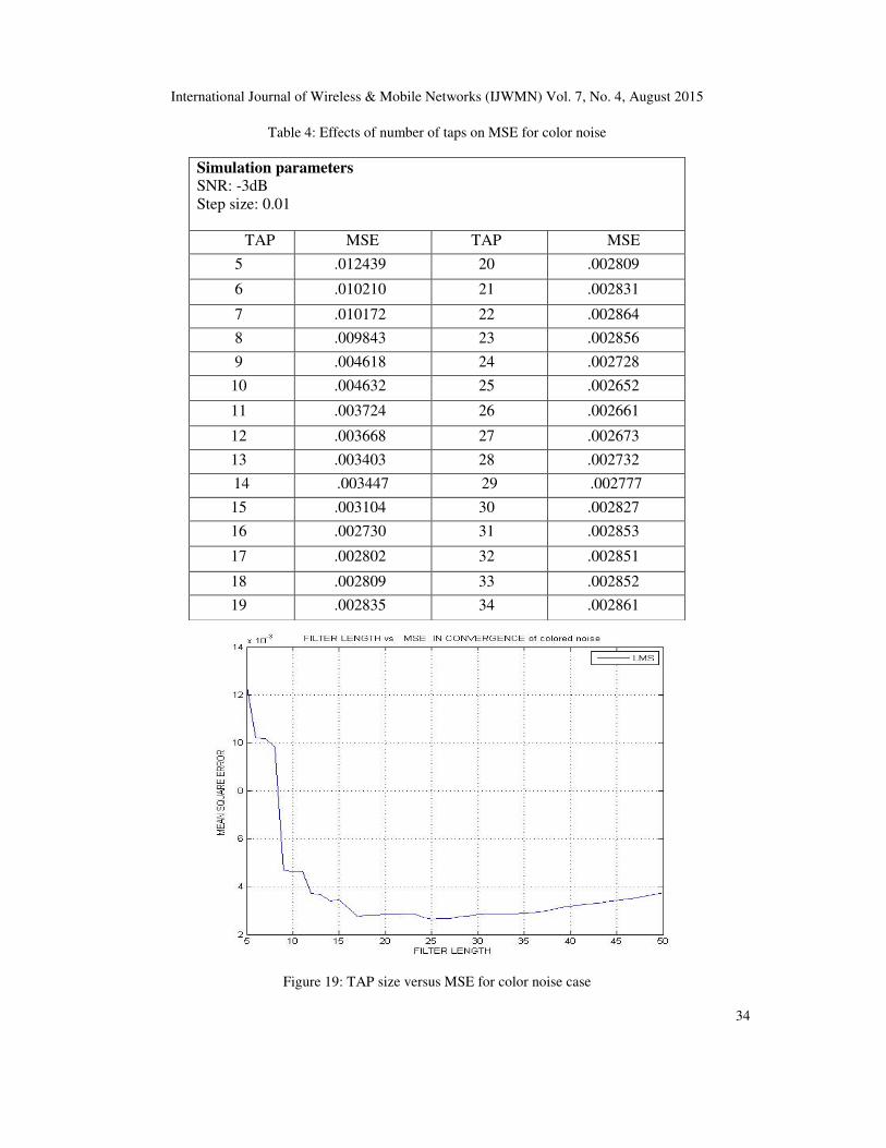
5.4. Effects of Tap Size on Mean Square Error (MSE)

The effects of tap size on MSE are tabulated in Table 3 (for white noise) and Table 4 (for color

noise) and the graphical representations of the results are shown in Fig. 18 (for white noise) and

Fig. 19 (for color noise). Fig. 18 illustrates that for white noise, the MSE linearly increases with

increasing tap size. For color noise as seen in Fig. 19, there is some initial randomness of the

values of MSE till a particular tap length (25) after which the MSE increases almost linearly with

increasing number of filter coefficients.


33

Table 3: Effects of number of taps on MSE for white noise

Simulation parameters

SNR: -3dB

Step size: 0.01

TAP

MSE TAP MSE

5 .001850 20 .002726

6 .001893 21 .002788

7 .001930 22 .002884

8 .001974 23 .002950

9 .002024 24 .003017

10 .002088 25 .003069

11 .002158 26 .003138

12 .002230 27 .003203

13 .002277 28 .003271

14 .002338 29 .003318

15 .002385 30 .003374

16 .002444 31 .003427

17 .002514 32 .003474

18 .002604 33 .003513

19 .002674 34 .003555

Figure 18: TAP size versus MSE for white noise case


34

Table 4: Effects of number of taps on MSE for color noise

Simulation parameters SNR: -3dB

Step size: 0.01

TAP MSE TAP MSE

5 .012439 20 .002809

6 .010210 21 .002831

7 .010172 22 .002864

8 .009843 23 .002856

9 .004618 24 .002728

10 .004632 25 .002652

11 .003724 26 .002661

12 .003668 27 .002673

13 .003403 28 .002732

14 .003447 29 .002777

15 .003104 30 .002827

16 .002730 31 .002853

17 .002802 32 .002851

18 .002809 33 .002852

19 .002835 34 .002861

Figure 19: TAP size versus MSE for color noise case


35

6.CONCLUSION

In this paper, we have considered white Gaussian noise and color noise to study the performance

of adaptive noise cancelling system. A comparison between the performances of Case 1 (for

white noise) and Case 2 (for color noise) is made as well as the effects of number of iterations,

SNR and tap size on the MSE are studied for both case. It is seen that the reduction of noise is

better and speed of convergence is faster for color noise as compared with white noise situation.

It has been found that MSE increased almost linearly with the filter length in case of white noise,

whereas for color noise, some initial randomness of the values of MSE is observed until a

particular tap length (25) after which the MSE increases almost linearly with increasing number

of filter coefficients. Our experiments to find the possible relationship between SNR and MSE

reveals that for both case, MSE decreases with increasing SNR with relatively faster decrease of

MSE in case of color noise compared with white noise. It is noticeable that at high SNR, better

MSE is obtained for Case 2. Our future plans include to study other adaptive algorithms and

analyse their effects on the performance of noise cancelling system.

REFERENCES

[1] E. C. Ifeachor and B. W. Jervis, Digital Signal Processing, Addison-Wesley Publishing Company,

1993.

[2] S. Haykin, Adaptive Filter Theory, 3RD edition, Prentice-Hall International Inc, 1996.

[3] F. Afroz, A. Huq, F. Ahmed and K. Sandrasegaran. “Performance Analysis of Adaptive Noise

Canceller Employing NLMS Algorithm,” International Journal of Wireless and Mobile Networks,

vol.7. no. 2, pp. 45-58, April 2015.

[4] B. Widrow and M.E. Hoff, “Adaptive switching circuits,” Proceedings of WESCON Convention

Record, part 4, pp.96-104, 1960.

[5] R. W. Harris, D.M. Chabries, and F. A. Bishop, “A variable step (VS) adaptive filter algorithm,”

IEEE Trans. Acoustics, Speech, Signal Processing, vol. ASSP-34, pp. 309-316, April 1986.

[6] A. Kanemasa and K. Niwa, “An adaptive-step sign algorithm for fast convergence of a data echo

canceller,” IEEE Trans. Communications, vol. COM-35, NO. 10, pp. 1102-1 106, October 1987.

[7] W. B. Mikhael et al., “Adaptive filters with individual adaptation of parameters,” IEEE Trans.

Circuits and Systems, vol. CAS-33, pp. 677-685, July 1986.

[8] V. J. Mathews and Z. Xie, “A stochastic gradient adaptive filter with gradient adaptive step size,”

IEEE Trans. Signal Processing, vol. 41, pp. 2075-2087, June 1993.

[9] M. H. Puder, and G.U. Schmidt, “Step-size control for acoustic echo cancellation filter-an overview,”

Signal Processing, pp. 1697-1719, September 2000.

[I0] S. Koike, “A class of adaptive step-size control algorithms for adaptive filters,” IEEE Trans. Signal

Processing, vol. 50, pp. 13 15- 1326, June 2002.

[11] B. Carter and R. Mancini, Op Amps for everyone, 3rd Edition, Texas Instruments, 2009.

[12] D.L. Rudnick and R.E. Davis, “Red noise and regime shifts,” Deep-Sea Research Part I, vol.50(6),

pp. 691-699, 2003.

[13] D.P. Mitchell, “Generating Antialiased Images at Low Sampling Densities,” ACM SIGGRAPH

Computer Graphics, vol.21(4), pp. 65-72, 1987.

[14] C. Roads, Composing Electronic Music: A New Aesthetic, Oxford University Press, May 2015.

[15] S.C. Douglas, “Introduction to Adaptive Filters” in Digital Signal Processing Handbook, Ed. Vijay

K. Madisetti and Douglas B. Williams, Boca Raton: CRC Press LLC, 1999.

[16] I. Ahmad, F. Ansari and U.K. Dey, “Cancellation of motion artifact noise and power line interference

in ECG using adaptive filters,” International Journal of Electronics Signals and Systems (IJESS),

Vol‐3, Iss‐2, pp 56-58, 2013.


36

[17] V. Anand, S. Shah and S. Kumar, “Intelligent Adaptive Filtering For Noise Cancellation,”

International Journal of Advanced Research in Electrical, Electronics and Instrumentation

Engineering, Vol. 2, Issue 5, pp. 2029-2039, May 2013.

[18] S. Yoon, S. Nat, S. Park, Y. Eom and S. Yoo, “Advanced Sound Capturing Method with Adaptive

Noise Reduction System for Broadcasting Multi copters,” IEEE International Conference on

Consumer Electronics, pp. 26-29, 2015.

[19] Siddappaji and K.L. Sudha, “Performance Analysis of New Time Varying LMS (NTVLMS)

Adaptive Filtering Algorithm in Noise Cancellation System,” International Conference on

Communication, Information & Computing Technology (ICCICT), pp. 1-6, 2015.

[20] G. Singh, K. Savia, S. Yadav and V. Purwar, “Design of adaptive noise canceller using LMS

algorithm,” International Journal of Advanced Technology & Engineering Research (IJATER), Vol.3,

Issue 3, May 2013.

[21] S. Haykin, “Least-Mean-Square Adaptive Filters,” in Adaptive Filter Theory, 4th Edition, Singapore,

Pearson Education, pp. 231-234, 2002.

cancellation of white and color noise with adaptive filter...

Documents