design for reliability concepts in accelerated testing ... accel testing.pdf · design for...
TRANSCRIPT
DESIGN for RELIABILITY Concepts in Accelerated Testing(DfRSoft.com - From our book Design for Reliability)
DfRSoft.com 1
9CONCEPTS IN ACCELERATED TESTING
9.1 INTRODUCTION
The concept of accelerated testing is to compress time and accelerate the failure
mechanisms in a reasonable test period so that product reliability can be assessed. The
only way to accelerate time is to stress potential failure modes. These include electrical
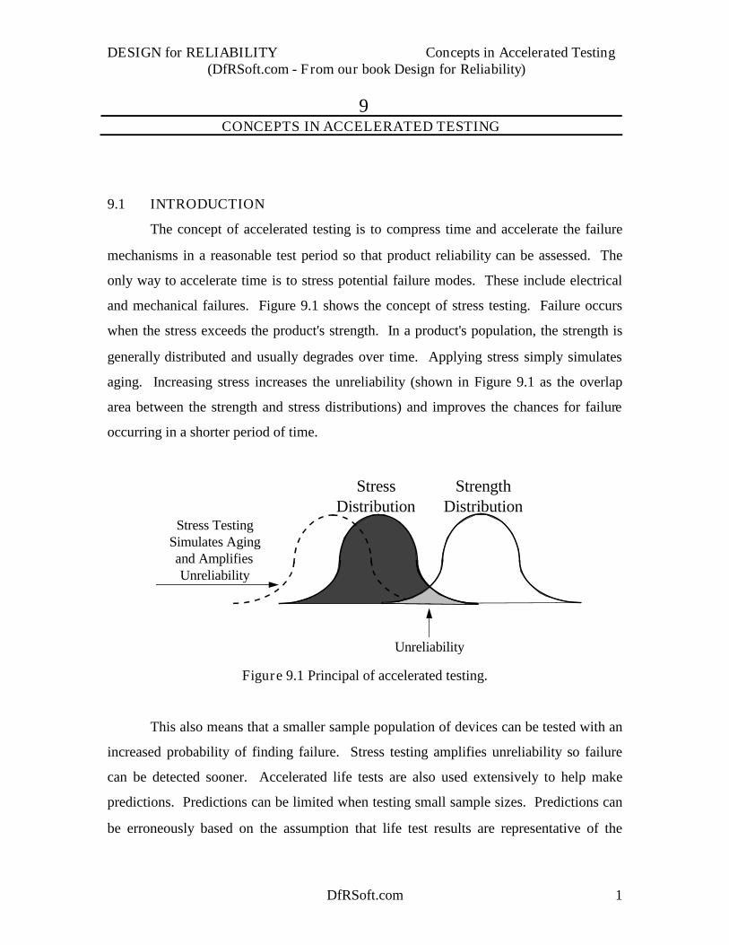
and mechanical failures. Figure 9.1 shows the concept of stress testing. Failure occurs
when the stress exceeds the product's strength. In a product's population, the strength is
generally distributed and usually degrades over time. Applying stress simply simulates
aging. Increasing stress increases the unreliability (shown in Figure 9.1 as the overlap
area between the strength and stress distributions) and improves the chances for failure
occurring in a shorter period of time.
Unreliability
Stress TestingSimulates Agingand AmplifiesUnreliability
StressDistribution
StrengthDistribution
Figure 9.1 Principal of accelerated testing.
This also means that a smaller sample population of devices can be tested with an
increased probability of finding failure. Stress testing amplifies unreliability so failure
can be detected sooner. Accelerated life tests are also used extensively to help make
predictions. Predictions can be limited when testing small sample sizes. Predictions can
be erroneously based on the assumption that life test results are representative of the
DESIGN for RELIABILITY Concepts in Accelerated Testing(DfRSoft.com - From our book Design for Reliability)
DfRSoft.com 2
entire population. Therefore, it can be difficult to design an efficient experiment that
yields enough failures so that the measures of uncertainty in the predictions are not too
large. Stresses can also be unrealistic. Fortunately, it is generally rare for an increased
stress to cause anomalous failures, especially if common sense guidelines are observed.
9.2 COMMON SENSE GUIDELINES FOR PREVENTING ANOMALOUS
ACCELERATED TESTING FAILURES
Anomalous failures can occur when testing pushes the limits of the material out of
the region of the intended design capability. The natural question to ask is this: What
should the guidelines be for designing proper accelerated tests and evaluating failures?
The answer is: Judgment is required by management and engineering staff to make the
correct decisions in this regard. To aid such decisions, the following guidelines are
provided:
1. Always refer to the literature to see what has been done in the area of accelerated
testing.
2. Avoid accelerated stresses that cause “nonlinearties”, unless such stresses are
plausible in product use conditions. Anomalous failures occur when accelerated
stress causes “nonlinearities” in the product. For example, material changing
phases from solid to liquid, as in a chemical “nonlinear” phase transition (e.g.,
solder melting, intermetallic changes, etc.); an electric spark in a material is an
electrical nonlinearity; material breakage compared to material flexing is a
mechanical nonlinearity.
3. Tests can be designed in two ways: by avoiding high stresses, or by allowing it,
which may or may not cause nonlinear stresses. In the latter test design, a
concurrent engineering design team reviews all failures and decides if a failure is
anomalous or not. Then a decision is made whether or not to fix the problem.
Conservative decisions may result in fixing some anomalous failures. This is not
a concern when time and money permit fixing all problems. The problem occurs
when normal failures are put in the wrong category as anomalous and no
corrective action is taken.

DESIGN for RELIABILITY Concepts in Accelerated Testing(DfRSoft.com - From our book Design for Reliability)
DfRSoft.com 3
9.3 TIME ACCELERATION FACTOR
The acceleration factor (A) is defined mathematically by Equation 9.1 where t is
the typical life of a failure mode under normal use conditions and t' is the life at
accelerated test condition:
'tt
A (9.1)
Since accelerated testing is designed to create failures in a shorter time frame, the
life under normal use conditions is usually much longer than the life under accelerated
test conditions, and A is much greater than 1. For example, an acceleration factor of 100
indicates that 1 hour in an accelerated stress environment is equal to 100 hours in the
normal use stress environment. Acceleration factors, as denoted here, describe time
compression. Acceleration factors may also be put in terms of parameter change. The
most common application is for estimating test time-compression using the time
acceleration factor.
Acceleration factors are often modeled. For example, many failure modes
affected by temperature, such as chemical processes and diffusion, have what is known as
an Arrhenius reaction rate given by
TK
EBRate
B
aexp(9.2)
where
B = a constant that characterizes the product failure mechanism and test conditions (see
Reference 1),
Ea = the activation energy in electron-volts (eV) of the failure mode,
T = the temperature (in degrees Kelvin), and
KB = Boltzmann's constant (8.617 10-5 eV/oK).
This is a thermodynamic expression that, while treated macroscopically to describe
failure kinetics, is obeyed in the microscopic world where elementary reactions are taking
place in accordance with the Arrhenius model. Particles have a certain probability to
DESIGN for RELIABILITY Concepts in Accelerated Testing(DfRSoft.com - From our book Design for Reliability)
DfRSoft.com 4
overcome the potential barrier of height Ea and become activated into the reaction taking
place. As more and more elementary particles are consumed, a catastrophic event takes
place at some point in the macroscopic world. The rate is assumed to be inversely
proportional to the time that this will occur. For example, if an experiment is performed
at two temperatures T1 and T2, the failure times are then related to the rates at these
temperatures as
tt
Rate TRate T
21
12
( )( )
(9.3)
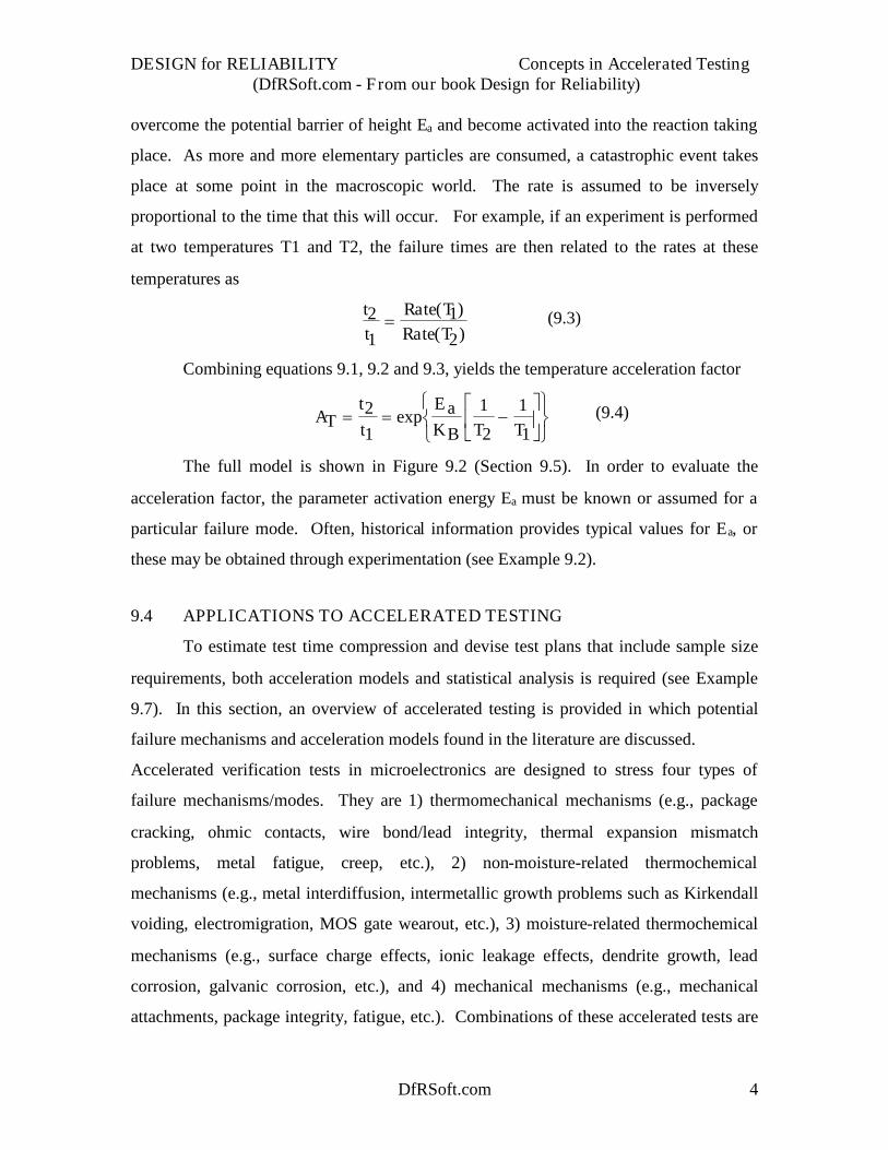
Combining equations 9.1, 9.2 and 9.3, yields the temperature acceleration factor
ATtt
E aK B T T
21
1
2
1
1exp (9.4)
The full model is shown in Figure 9.2 (Section 9.5). In order to evaluate the
acceleration factor, the parameter activation energy Ea must be known or assumed for a
particular failure mode. Often, historical information provides typical values for Ea, or
these may be obtained through experimentation (see Example 9.2).
9.4 APPLICATIONS TO ACCELERATED TESTING
To estimate test time compression and devise test plans that include sample size
requirements, both acceleration models and statistical analysis is required (see Example
9.7). In this section, an overview of accelerated testing is provided in which potential
failure mechanisms and acceleration models found in the literature are discussed.
Accelerated verification tests in microelectronics are designed to stress four types of
failure mechanisms/modes. They are 1) thermomechanical mechanisms (e.g., package
cracking, ohmic contacts, wire bond/lead integrity, thermal expansion mismatch
problems, metal fatigue, creep, etc.), 2) non-moisture-related thermochemical
mechanisms (e.g., metal interdiffusion, intermetallic growth problems such as Kirkendall
voiding, electromigration, MOS gate wearout, etc.), 3) moisture-related thermochemical
mechanisms (e.g., surface charge effects, ionic leakage effects, dendrite growth, lead
corrosion, galvanic corrosion, etc.), and 4) mechanical mechanisms (e.g., mechanical
attachments, package integrity, fatigue, etc.). Combinations of these accelerated tests are
DESIGN for RELIABILITY Concepts in Accelerated Testing(DfRSoft.com - From our book Design for Reliability)
DfRSoft.com 5
required to properly stress each failure mechanism. The most common tests are
Temperature cycle, High Temperature Operating Life (HTOL), Temperature Humidity
Bias (THB), and Vibration testing, which are described here. Additionally,
electromigration testing is described in this chapter. Temperature cycle stresses
thermomechanical mechanisms; HTOL stresses non-moisture-related thermochemical
mechanisms; THB stresses moisture-related thermochemical mechanisms; and vibration
stresses mechanical failure mechanisms.
Additionally, many devices during manufacture receive some manufacturing
stress. For example, surface-mount-technology (SMT) devices are subject to solder-
reflow processes. Therefore, to provide a realistic verification test procedure prior to
accelerated reliability testing, devices should receive a preconditining to simulate these
stresses. In the case of SMT devices, a solder-reflow-type preconditioning test, such as
described in JEDEC specification JESD22-A113, is commonly used.
9.5 HIGH-TEMPERATURE LIFE TEST ACCELERATION MODEL
In high-temperature life testing, devices are subjected to elevated temperature
under bias for an extended period of time. Often, it is assumed that the dominant
thermally accelerated failure mechanisms will follow the classical Arrhenius relationship
(previously discussed). The traditional HTOL Arrhenius acceleration model is provided
in Figure 9.2. The Arrhenius function is important. It is not only used in reliability to
model temperature-dependent failure-rate mechanisms, but expresses a number of
different physical thermodynamic phenomena (see Chapter 14). In Equation 9.2, we see
that this factor is exponentially related to the activation energy. As the name connotes, in
the failure process there must be enough thermal energy to be activated and surmount the
potential barrier height of value Ea. Thus, as the temperature increases, it is easier to
surmount this barrier and increase the probability of failure in a shorter time period.
Thus, the activation energy parameter expresses a characteristic value that can be related
to thermally activated failure processes. Each failure process has associated with it a
barrier height Ea. In practice, when trying to estimate acceleration factor without
knowing this value for each potential failure mechanism, a conservative value is used.
DESIGN for RELIABILITY Concepts in Accelerated Testing(DfRSoft.com - From our book Design for Reliability)
DfRSoft.com 6
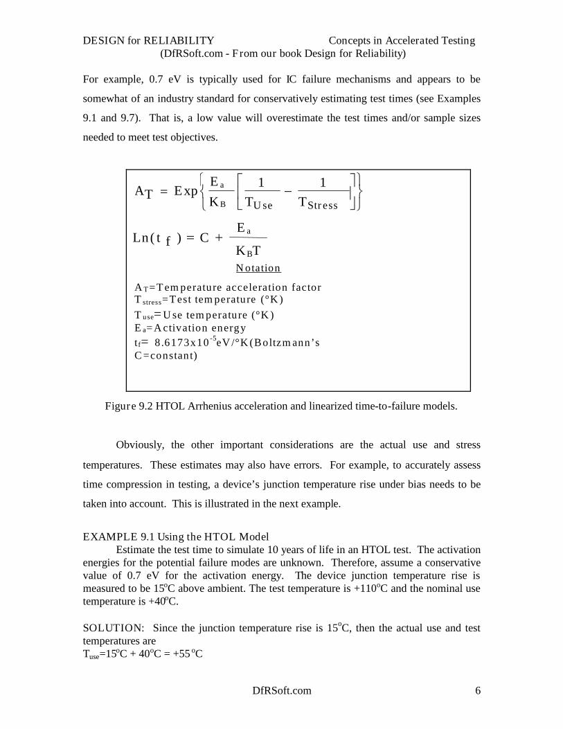
For example, 0.7 eV is typically used for IC failure mechanisms and appears to be
somewhat of an industry standard for conservatively estimating test times (see Examples
9.1 and 9.7). That is, a low value will overestimate the test times and/or sample sizes
needed to meet test objectives.
N otation
A T=T em perature acceleration factorT stress=Test tem perature (°K )T use= U se tem perature (°K )E a=A ctivation energytf= 8.6173x10 -5eV /°K (Boltzm ann’sC =constant)= T im e to fail
A T ExpE a
K B TU se T Stress
1 1
Ln t f CE a
K BT( )
Figure 9.2 HTOL Arrhenius acceleration and linearized time-to-failure models.
Obviously, the other important considerations are the actual use and stress
temperatures. These estimates may also have errors. For example, to accurately assess
time compression in testing, a device’s junction temperature rise under bias needs to be
taken into account. This is illustrated in the next example.
EXAMPLE 9.1 Using the HTOL ModelEstimate the test time to simulate 10 years of life in an HTOL test. The activation
energies for the potential failure modes are unknown. Therefore, assume a conservativevalue of 0.7 eV for the activation energy. The device junction temperature rise ismeasured to be 15oC above ambient. The test temperature is +110oC and the nominal usetemperature is +40oC.
SOLUTION: Since the junction temperature rise is 15oC, then the actual use and testtemperatures areTuse=15oC + 40oC = +55 oC

DESIGN for RELIABILITY Concepts in Accelerated Testing(DfRSoft.com - From our book Design for Reliability)
DfRSoft.com 7
TStress=15 oC + 110oC = +125 oCFrom Figure 9.2, the acceleration factor isA T= Exp {(0.7 eV/8.6173x10-5 eV/oK)[1/(273.15+55) - 1/(273.15+125) oK]} = 77.6From Equation 9.1, the test time to simulate 10 years of life (87,600 hours) isTest Time=Life Time/AT=87600/77.6=1,129 hours
9.5.1 Estimating Activation Energy
Tests are often performed to determine a failure mechanism’s activation energy.
In this case, devices are separately tested in at least two different temperatures. Ideally,
three or more temperatures can be used, then test results can be plotted on a semilog
graph and the data fitted using a least-squares method. An example is the process
reliability study shown in Figure 6.8 where a semilog plot is used related to the linearized
model in Figure 9.2. That is, if we plot the Mean Time To Failure (MTTF) on the
semilog axis versus 1/T, then according to the equation
TK
EConstMTTFLn
B
a 1)(
(9.5)
the slope is Ea/KB and the activation energy can be determined as illustrated in the next
example.
EXAMPLE 9.2 Determining the Activation EnergyThe MTTFs at +250oC and +200oC are 731 and 10,400 hours, respectively, in
Figure 6.8. Show that the activation energy is 1.13 eV and that the MTTF at +125oC is1.95 106 hours as indicated in the figure.
SOLUTION: Equation 9.4 can be solved for Ea as
12
12/1/1
/TT
MTTFMTTFLnKE Ba
(9.6)
Then, the activation energy is
1.133eVK250)]+1/(273.16-200)+[1/(273.16
731]/[10400LnKeV/8.6173x10o
o5- aE
Next, the acceleration factor at +125oC must be determined. Using the procedure inExample 9.1, we have
Tuse= +125oCTStress= +200oC
A T= Exp {(1.133 eV/8.6171x10-5 eV/oK)[1/(273.15+125) - 1/(273.15+200) oK]} =187.6

DESIGN for RELIABILITY Concepts in Accelerated Testing(DfRSoft.com - From our book Design for Reliability)
DfRSoft.com 8
From Equation 9.1, the MTTF (at +125C) = MTTF (at +200C) AT = 10400 187.7 =1.951 106 hours. The answer is a bit off to the value shown in Fig. 6.8, due to round-offerror.
9.6 THB ACCELERATION MODEL
In THB, test devices are put at elevated temperatures and humidity under bias for
an extended period of time. For example, the most common THB test is a 1000-hour test
at +85oC and 85% Relative Humidity. One of the most common THB models used in the
industry is a 1989 Peck model (see Reference 3) shown in Figure 9.3. A derivation is
provided in Chapter 14, Section 14.5.2. This includes a relationship between life and
temperature (Arrhenius model) and life-and-humidity (Peck model), so that the product of
the two separable factors yields an overall acceleration factor.
NotationAH = Humidity acceleration FactorAT = Temperature acceleration factorATH = Temperature-Humidity acceleration factorRHstress = Relative humidity of testRHuse = Nominal use relative humidityTstress = Test temperatureTuse = Nominal use temperaturem = Humidity constantEa = Activation energytf = Time to FailC = Constant
AT ExpEa
K TUse TStress
1 1
AHRStress
RUse
m
ATH=AT AH
Ln t f CE a
KB Tm Ln R( )
B
Figure 9.3 THB Peck acceleration and linearized time to failure models.
EXAMPLE 9.3 Using the THB ModelIf a THB test is performed at 85%RH and +85oC, what is the acceleration factor
relative to a 40%RH and +25oC environment, assuming an activation energy of 0.7 eV
DESIGN for RELIABILITY Concepts in Accelerated Testing(DfRSoft.com - From our book Design for Reliability)
DfRSoft.com 9
and a humidity constant of 2.66? How many test hours are required to simulate 10 yearsof life? How many test hours are required in a HAST chamber (see Chapter 5) tosimulate 10 years of life at 85%RH and +110 oC?
SOLUTION: The temperature acceleration factor isA T= exp {(0.7eV/8.6173x10-5 eV/oK)*[1/(273.15+25) - 1/(273.15+85) oK]} = 96
The humidity acceleration factor isA H= (85%RH/40%RH)2.66 = 7.43
Therefore, the combined temperature humidity acceleration factor isATH =967.43 = 713
The simulated test time to equate this to 10 years (87,600 hours) isTest time= (87,600 hours / 713) = 123 hours
The temperature acceleration factor for the HAST test isA T= exp {(0.7 eV/8.617310-5 eV/oK)[1/(273.15+25) - 1/(273.15+110) oK]} = 421.8
The humidity acceleration factor is the same as in the first part of the problem so thatATH =421.87.43 = 3132.2
The simulated test time to equate this HAST test to10 years isHAST test time= (87600 hours/3132) = 28 hours
When Peck originally proposed this model, he reviewed all published life-in-
humidity conditions versus life at +85oC/85%RH for epoxy packages. His results found
good agreement with the model. Fitted data found nominal values for Ea to lie between
0.77 and 0.81 and nominal values between 2.5 and 3.0 for m. A thorough study by Texas
Instruments (see Reference 4) on PEM moisture-life monitoring, found the activation
energy values up around 0.9 eV. Such trends in the literature indicate higher-activation
energies, which correspond to trends in improved semiconductor reliability.
9.7 TEMPERATURE CYCLE ACCELERATION MODEL
In Temperature Cycle, test devices are subjected to a number of cycles of alternate
high and low temperature extremes. This cyclic stress produced in temperature cycling is
related to thermal expansion and contraction undergone in the material. To relate field
usage to accelerated test conditions, the most widely used model in industry is the Coffin-
Manson (see Reference 1) model. This is a simple model used for estimating the
temperature cycle acceleration factor (see Figure 9.4). A derivation of this model is
provided in Chapter 14, Section 14.4.2.
Reasonably estimating the acceleration factor depends on the failures being
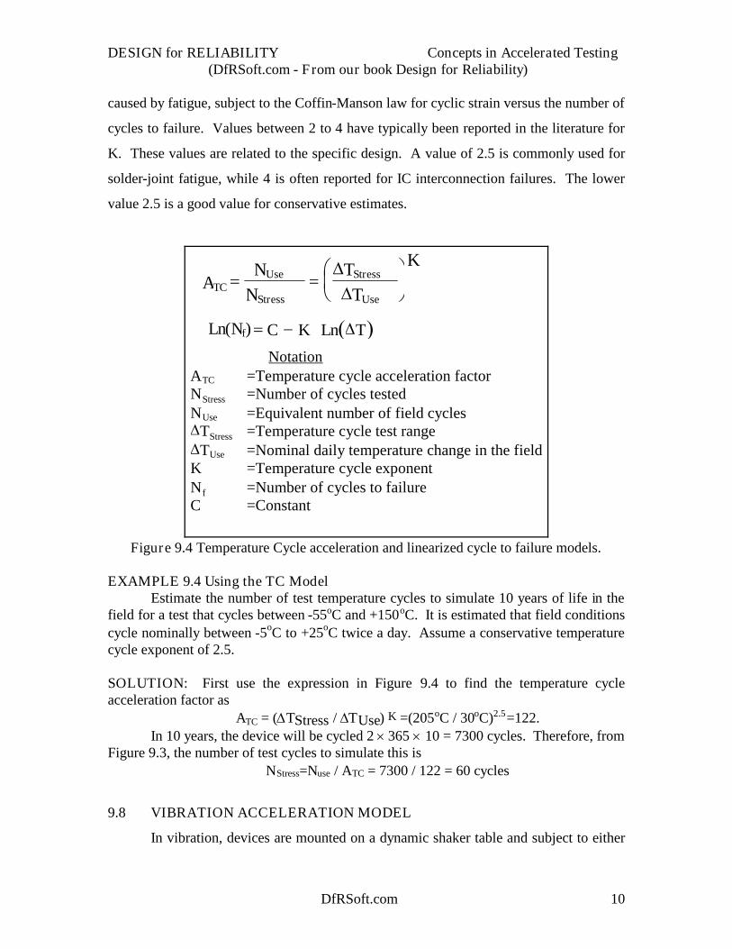
DESIGN for RELIABILITY Concepts in Accelerated Testing(DfRSoft.com - From our book Design for Reliability)
DfRSoft.com 10
caused by fatigue, subject to the Coffin-Manson law for cyclic strain versus the number of
cycles to failure. Values between 2 to 4 have typically been reported in the literature for
K. These values are related to the specific design. A value of 2.5 is commonly used for
solder-joint fatigue, while 4 is often reported for IC interconnection failures. The lower
value 2.5 is a good value for conservative estimates.
NotationATC =Temperature cycle acceleration factorNStress =Number of cycles testedNUse =Equivalent number of field cyclesTStress =Temperature cycle test rangeTUse =Nominal daily temperature change in the fieldK =Temperature cycle exponentNf =Number of cycles to failureC =Constant
ATCNUse
NStress
TStress
TUse
K
Ln(Nf) C K Ln T
Figure 9.4 Temperature Cycle acceleration and linearized cycle to failure models.
EXAMPLE 9.4 Using the TC ModelEstimate the number of test temperature cycles to simulate 10 years of life in the
field for a test that cycles between -55oC and +150oC. It is estimated that field conditionscycle nominally between -5oC to +25oC twice a day. Assume a conservative temperaturecycle exponent of 2.5.
SOLUTION: First use the expression in Figure 9.4 to find the temperature cycleacceleration factor as
ATC = (TStress / TUse) K =(205oC / 30oC)2.5=122.In 10 years, the device will be cycled 2 365 10 = 7300 cycles. Therefore, from
Figure 9.3, the number of test cycles to simulate this isNStress=Nuse / ATC = 7300 / 122 = 60 cycles
9.8 VIBRATION ACCELERATION MODEL
In vibration, devices are mounted on a dynamic shaker table and subject to either
DESIGN for RELIABILITY Concepts in Accelerated Testing(DfRSoft.com - From our book Design for Reliability)
DfRSoft.com 11
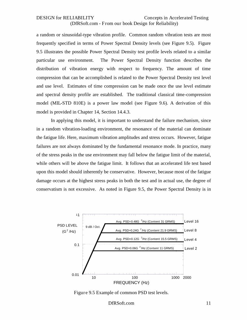
a random or sinusoidal-type vibration profile. Common random vibration tests are most
frequently specified in terms of Power Spectral Density levels (see Figure 9.5). Figure
9.5 illustrates the possible Power Spectral Density test profile levels related to a similar
particular use environment. The Power Spectral Density function describes the
distribution of vibration energy with respect to frequency. The amount of time
compression that can be accomplished is related to the Power Spectral Density test level
and use level. Estimates of time compression can be made once the use level estimate
and spectral density profile are established. The traditional classical time-compression
model (MIL-STD 810E) is a power law model (see Figure 9.6). A derivation of this
model is provided in Chapter 14, Section 14.4.3.
In applying this model, it is important to understand the failure mechanism, since
in a random vibration-loading environment, the resonance of the material can dominate
the fatigue life. Here, maximum vibration amplitudes and stress occurs. However, fatigue
failures are not always dominated by the fundamental resonance mode. In practice, many
of the stress peaks in the use environment may fall below the fatigue limit of the material,
while others will be above the fatigue limit. It follows that an accelerated life test based
upon this model should inherently be conservative. However, because most of the fatigue
damage occurs at the highest stress peaks in both the test and in actual use, the degree of
conservatism is not excessive. As noted in Figure 9.5, the Power Spectral Density is in
0.01
0.1
1
10 100 1000
PSD LEVEL
(G 2 /Hz)
FREQUENCY (Hz)
Avg. PSD=0.12G 2/Hz (Content 15.5 GRMS)
Avg. PSD=0.06G 2 /Hz (Content 11 GRMS)
Avg. PSD=0.24G 2 /Hz (Content 21.9 GRMS)
Avg. PSD=0.48G 2/Hz (Content 31 GRMS) Level 16
Level 8
Level 4
Level 2
9 dB / Oct.
2000
1
Figure 9.5 Example of common PSD test levels.
DESIGN for RELIABILITY Concepts in Accelerated Testing(DfRSoft.com - From our book Design for Reliability)
DfRSoft.com 12
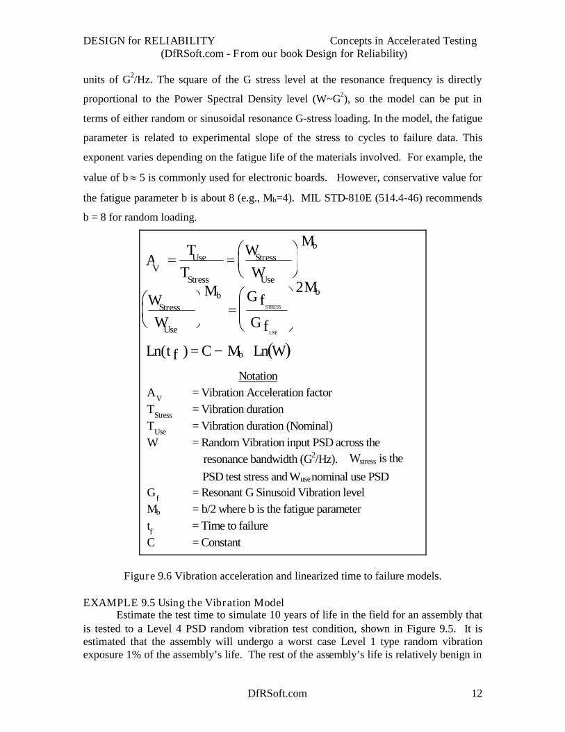
units of G2/Hz. The square of the G stress level at the resonance frequency is directly
proportional to the Power Spectral Density level (W~G2), so the model can be put in
terms of either random or sinusoidal resonance G-stress loading. In the model, the fatigue
parameter is related to experimental slope of the stress to cycles to failure data. This
exponent varies depending on the fatigue life of the materials involved. For example, the
value of b 5 is commonly used for electronic boards. However, conservative value for
the fatigue parameter b is about 8 (e.g., Mb=4). MIL STD-810E (514.4-46) recommends
b = 8 for random loading.
NotationAV = Vibration Acceleration factorTStress = Vibration durationTUse = Vibration duration (Nominal)W = Random Vibration input PSD across the
resonance bandwidth (G2/Hz). Wstress is the
PSD test stress and Wusenominal use PSDGf = Resonant G Sinusoid Vibration levelMb = b/2 where b is the fatigue parametertf = Time to failureC = Constant
AV
TUse
TStress
WStress
WUse
Mb
Ln t f C Mb Ln W( )
WStress
WUse
Mb G fG f
MbSTRESS
USE
2
Figure 9.6 Vibration acceleration and linearized time to failure models.
EXAMPLE 9.5 Using the Vibration ModelEstimate the test time to simulate 10 years of life in the field for an assembly that
is tested to a Level 4 PSD random vibration test condition, shown in Figure 9.5. It isestimated that the assembly will undergo a worst case Level 1 type random vibrationexposure 1% of the assembly’s life. The rest of the assembly’s life is relatively benign in
DESIGN for RELIABILITY Concepts in Accelerated Testing(DfRSoft.com - From our book Design for Reliability)
DfRSoft.com 13
terms of vibration exposure.
SOLUTION: First use the expression in Figure 9.6 to find the vibration accelerationfactor. Since Level 4 has a PSD of 0.12 G2/Hz, then Level 1 is 0.03 G2/Hz. Therefore,
AV= (WStress / WUse) Mb=(0.12/ 0.03)4 = 256.In 10 years, the device will be exposed to a Level 1 vibration for about 87,600 0.01 =876 hours. Therefore, from Figure 9.6, the number of test cycles to simulate this isTStress=Tuse / AV = 876 / 256 = 3.5 hours.
9.9 ELECTROMIGRATION ACCELERATION MODEL
Electromigration is a failure mechanism caused in a microelectronic conductor
exposed to high current densities or a combination of high temperature and current density.
The most common failure mode is a conductor open. This failure mechanism comes about
from high current densities that create crowded electron flux in the microelectronic
conductive path. Often, the term “electron wind” has been historically used for the
scattering mechanism causing failure. The metal reaches a stage at which collision between
the electrons and film atoms and defects sites becomes catastrophic. Electron scattering
from defect sites is considered to dominate. The collision rate increases to the point that
atoms of the metal film drift in the direction of the electron flow. Eventual catastrophic
problems result due to local inhomogenous regions in the metal combined with the metal
movement.
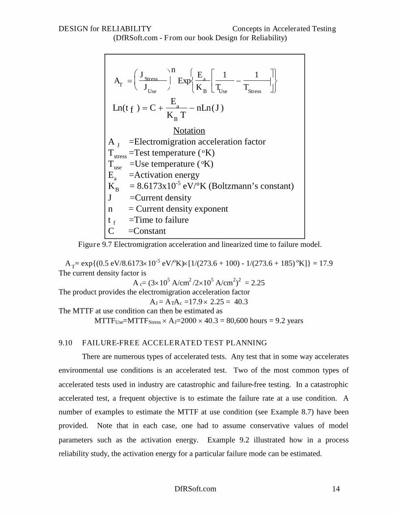
Generally, the Black equation (see Reference 6 and 7) is widely used for making
MTTF electromigration predictions in the literature. For the electromigration acceleration
factor due to the Black equation, see Figure 9.7. Numerous values for the Black equation
parameters n and Ea have been reported in the literature. As lower values are used, the
estimates become more conservative. Numerous experiments have been performed under
various stress conditions in the literature and values for n have been reported in the range
between 2 and 3.3 and between 0.5 to 1.1 eV for Ea.
EXAMPLE 9.6 Using the Electromigration ModelAn electromigration experiment performed on aluminum conductors at +185oC and a
current density of 3 105 A/cm2 found a MTTF of 2000 hours. Estimate the MTTF at a usecondition of +100oC and a current density of 2 105 A/cm2. Use conservative parameterestimates of Ea = 0.5 eV and n = 2.0.
SOLUTION: First find the temperature acceleration factor, which is
DESIGN for RELIABILITY Concepts in Accelerated Testing(DfRSoft.com - From our book Design for Reliability)
DfRSoft.com 14
A T= exp{(0.5 eV/8.617310-5 eV/oK)[1/(273.6 + 100) - 1/(273.6 + 185) oK]} = 17.9The current density factor is
A c= (3105 A/cm2 /2105 A/cm2)2 = 2.25The product provides the electromigration acceleration factor
AJ = ATAc =17.92.25 = 40.3The MTTF at use condition can then be estimated as
MTTFUse=MTTFStress AJ=2000 40.3 = 80,600 hours = 9.2 years
9.10 FAILURE-FREE ACCELERATED TEST PLANNING
There are numerous types of accelerated tests. Any test that in some way accelerates
environmental use conditions is an accelerated test. Two of the most common types of
accelerated tests used in industry are catastrophic and failure-free testing. In a catastrophic
accelerated test, a frequent objective is to estimate the failure rate at a use condition. A
number of examples to estimate the MTTF at use condition (see Example 8.7) have been
provided. Note that in each case, one had to assume conservative values of model
parameters such as the activation energy. Example 9.2 illustrated how in a process
reliability study, the activation energy for a particular failure mode can be estimated.
NotationA J =Electromigration acceleration factorTstress =Test temperature ( oK)Tuse =Use temperature ( oK)Ea =Activation energyKB = 8.6173x10⁻⁵ eV/°K (Boltzmann’s constant)J =Current densityn = Current density exponentt f =Time to failureC =Constant
AT
JStress
JUse
nExp
Ea
K B TUse TStress
1 1
Ln t f CE
a
K B TnLn J( ) ( )
Figure 9.7 Electromigration acceleration and linearized time to failure model.
DESIGN for RELIABILITY Concepts in Accelerated Testing(DfRSoft.com - From our book Design for Reliability)
DfRSoft.com 15
In Chapter 4, Design Maturity Testing (DMT) was discussed. DMT is based on
failure-free testing. The main objective of a DMT test is to determine whether a design will
meet its reliability objective at a certain level of confidence. This requires that a statistically
significant sample size be tested in a number of different stress tests. This topic was
introduced in Section 4.6. In Chapter 8, an example was provided on accelerated
demonstration versus statistical sample planning. However, at this point, we would like to
illustrate how to conservatively plan a DMT to demonstrate that a particular reliability
objective can be met.
EXAMPLE 9.7 Designing a Failure-Free Accelerated TestPlan accelerated tests for a failure-free DMT to demonstrate that a plastic-packaged
IC will meet its reliability objective of 400 FITs (Objective 4, Figure 4.3) at the 90%confidence level. Estimate the sample size required and test times needed to show that thiscomponent is failure-free of any HTOL, THB, and TC type failure modes. Use theacceleration factors found in Examples 9.1, 9.3, and 9.4 in your design.
SOLUTION: A full DMT test for this component will include nonaccelerated tests as well.Figure 4.5 illustrates the concept and Chapter 4 describes DMT in detail. To design theaccelerated testing portion, first estimate a practical test duration. For example, we cantarget the test to last about a 1000 hours for HTOL and THB, and about 100 temperaturecycles. Once we have fixed the test time, we next must estimate a statistically significantsample size at the 90% confidence level. We can assume that each test will check fordifferent failure modes. This means that each test should be allocated a portion of the failurerate. One allocation plan is described in Section 4.2 where THB, TC, and HTOL typefailure modes were assigned 20, 30, and 50% respectively of the total reliability. Using thisplan, the 400 FITs is broken up with 80, 120, and 200 FITs to THB, TC, and HTOL tests,respectively. At this point, a single-sided chi-square estimate for sample size planning canbe used. This is detailed in Section 4.6 where the sample size N is given
N(HTOL)=(90%, 2Y+2)/2AtFor example, the TC values areY=0 Failures(90%, 2)=4.605=120 FITs=1.2 x 10⁻⁷ failure/hourA=122 (from Example 9.4)t=100 cycles x 24 Hours=2400 equivalent test hoursThus,
N=4.605/(21.210-7122 2400)=66 devicesUsing this same approach for the other tests, the results are summarizes below.
Table 9.1 Summary of DMT Test for Example 9.8
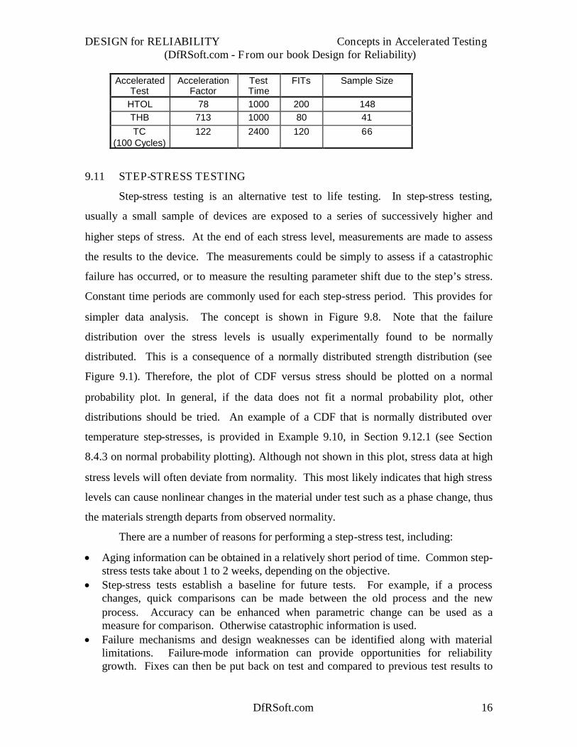
DESIGN for RELIABILITY Concepts in Accelerated Testing(DfRSoft.com - From our book Design for Reliability)
DfRSoft.com 16
AcceleratedTest
AccelerationFactor
TestTime
FITs Sample Size
HTOL 78 1000 200 148THB 713 1000 80 41TC
(100 Cycles)122 2400 120 66
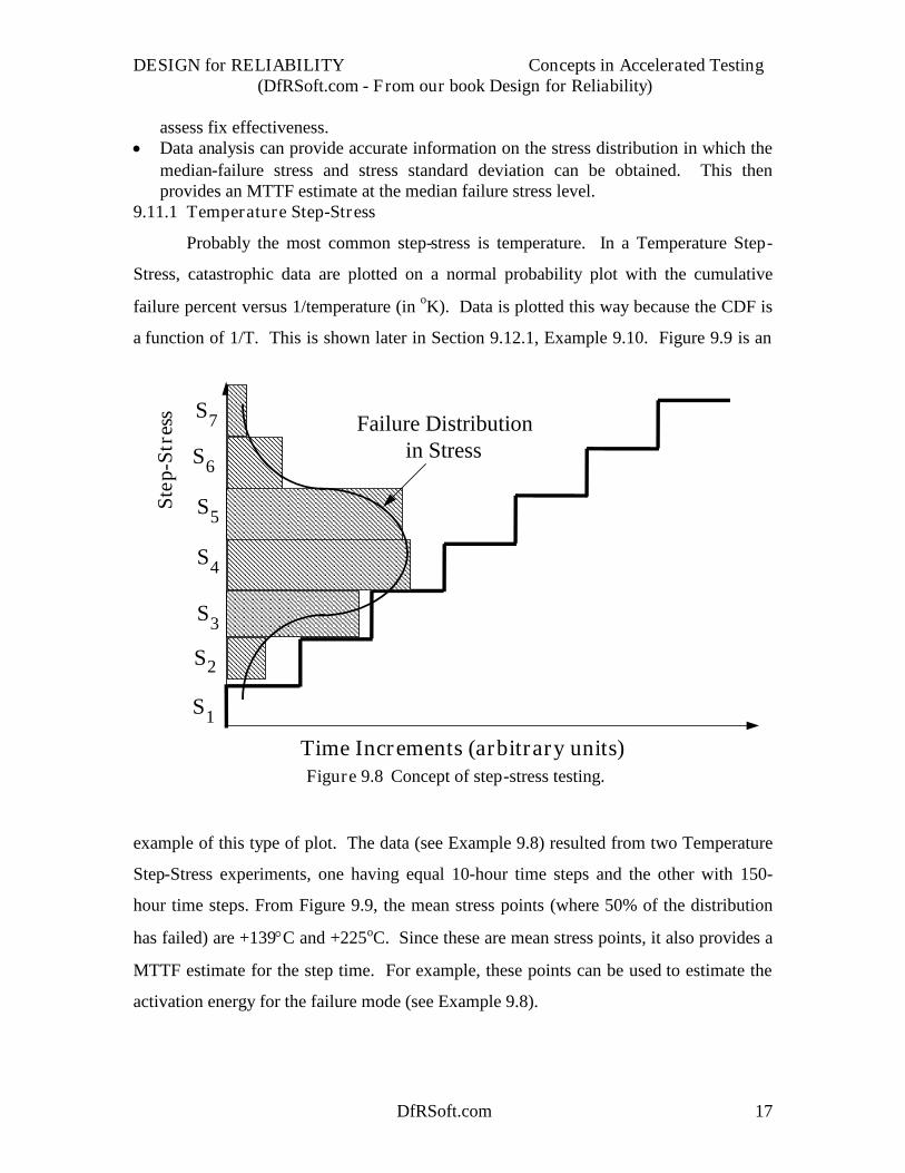
9.11 STEP-STRESS TESTING
Step-stress testing is an alternative test to life testing. In step-stress testing,
usually a small sample of devices are exposed to a series of successively higher and
higher steps of stress. At the end of each stress level, measurements are made to assess
the results to the device. The measurements could be simply to assess if a catastrophic
failure has occurred, or to measure the resulting parameter shift due to the step’s stress.
Constant time periods are commonly used for each step-stress period. This provides for
simpler data analysis. The concept is shown in Figure 9.8. Note that the failure
distribution over the stress levels is usually experimentally found to be normally
distributed. This is a consequence of a normally distributed strength distribution (see
Figure 9.1). Therefore, the plot of CDF versus stress should be plotted on a normal
probability plot. In general, if the data does not fit a normal probability plot, other
distributions should be tried. An example of a CDF that is normally distributed over
temperature step-stresses, is provided in Example 9.10, in Section 9.12.1 (see Section
8.4.3 on normal probability plotting). Although not shown in this plot, stress data at high
stress levels will often deviate from normality. This most likely indicates that high stress
levels can cause nonlinear changes in the material under test such as a phase change, thus
the materials strength departs from observed normality.
There are a number of reasons for performing a step-stress test, including:
Aging information can be obtained in a relatively short period of time. Common step-stress tests take about 1 to 2 weeks, depending on the objective.
Step-stress tests establish a baseline for future tests. For example, if a processchanges, quick comparisons can be made between the old process and the newprocess. Accuracy can be enhanced when parametric change can be used as ameasure for comparison. Otherwise catastrophic information is used.
Failure mechanisms and design weaknesses can be identified along with materiallimitations. Failure-mode information can provide opportunities for reliabilitygrowth. Fixes can then be put back on test and compared to previous test results to
DESIGN for RELIABILITY Concepts in Accelerated Testing(DfRSoft.com - From our book Design for Reliability)
DfRSoft.com 17
assess fix effectiveness. Data analysis can provide accurate information on the stress distribution in which the
median-failure stress and stress standard deviation can be obtained. This thenprovides an MTTF estimate at the median failure stress level.
9.11.1 Temperature Step-Stress
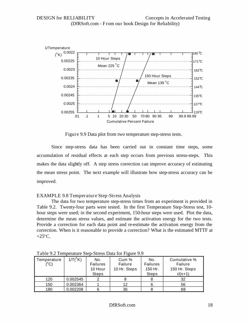
Probably the most common step-stress is temperature. In a Temperature Step-
Stress, catastrophic data are plotted on a normal probability plot with the cumulative
failure percent versus 1/temperature (in oK). Data is plotted this way because the CDF is
a function of 1/T. This is shown later in Section 9.12.1, Example 9.10. Figure 9.9 is an
example of this type of plot. The data (see Example 9.8) resulted from two Temperature
Step-Stress experiments, one having equal 10-hour time steps and the other with 150-
hour time steps. From Figure 9.9, the mean stress points (where 50% of the distribution
has failed) are +139C and +225oC. Since these are mean stress points, it also provides a
MTTF estimate for the step time. For example, these points can be used to estimate the
activation energy for the failure mode (see Example 9.8).
S1
S2
S3
S4
S5
S6
S7
Step
-Str
ess Failure Distribution
in Stress
Time Increments (arbitrary units)Figure 9.8 Concept of step-stress testing.
DESIGN for RELIABILITY Concepts in Accelerated Testing(DfRSoft.com - From our book Design for Reliability)
DfRSoft.com 18
Since step-stress data has been carried out in constant time steps, some
accumulation of residual effects at each step occurs from previous stress-steps. This
makes the data slightly off. A step stress correction can improve accuracy of estimating
the mean stress point. The next example will illustrate how step-stress accuracy can be
improved.
EXAMPLE 9.8 Temperature Step-Stress AnalysisThe data for two temperature step-stress times from an experiment is provided in
Table 9.2. Twenty-four parts were tested. In the first Temperature Step-Stress test, 10-hour steps were used; in the second experiment, 150-hour steps were used. Plot the data,determine the mean stress values, and estimate the activation energy for the two tests.Provide a correction for each data point and re-estimate the activation energy from thecorrection. When is it reasonable to provide a correction? What is the estimated MTTF at+25C.
Table 9.2 Temperature Step-Stress Data for Figure 9.9Temperature
(oC)1/T(oK) No.
Failures10 HourSteps
Cum %Failure
10 Hr. Steps
No.Failures150 Hr.Steps
Cumulative %Failure
150 Hr. Stepsi/(n+1)
120 0.002545 2 8 8 32150 0.002364 1 12 6 56180 0.002208 6 36 8 88
0.0022
0.00225
0.0023
0.00235
0.0024
0.00245
0.0025
0.00255.01 .1 1 5 10 20 30 50 70 80 90 95 99 99.9 99.99
1/Temperature
(oK)
Cumulative Percent Failure
10 Hour Steps
Mean 225oC
150 Hour Steps
Mean 139 oC
180 oC
152oC
144oC
135oC
127oC
119oC
162oC
171oC
Figure 9.9 Data plot from two temperature step-stress tests.
DESIGN for RELIABILITY Concepts in Accelerated Testing(DfRSoft.com - From our book Design for Reliability)
DfRSoft.com 19
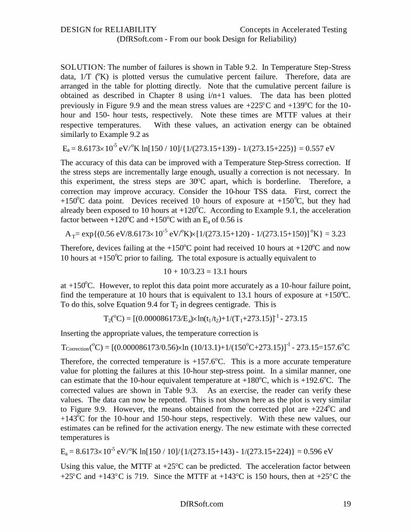
SOLUTION: The number of failures is shown in Table 9.2. In Temperature Step-Stressdata, 1/T (oK) is plotted versus the cumulative percent failure. Therefore, data arearranged in the table for plotting directly. Note that the cumulative percent failure isobtained as described in Chapter 8 using i/n+1 values. The data has been plottedpreviously in Figure 9.9 and the mean stress values are +225C and +139oC for the 10-hour and 150- hour tests, respectively. Note these times are MTTF values at theirrespective temperatures. With these values, an activation energy can be obtainedsimilarly to Example 9.2 as
Ea = 8.617310-5 eV/oK ln[150 / 10]/{1/(273.15+139) - 1/(273.15+225)} = 0.557 eV
The accuracy of this data can be improved with a Temperature Step-Stress correction. Ifthe stress steps are incrementally large enough, usually a correction is not necessary. Inthis experiment, the stress steps are 30OC apart, which is borderline. Therefore, acorrection may improve accuracy. Consider the 10-hour TSS data. First, correct the+150oC data point. Devices received 10 hours of exposure at +150oC, but they hadalready been exposed to 10 hours at +120oC. According to Example 9.1, the accelerationfactor between +120oC and +150oC with an Ea of 0.56 is
A T= exp{(0.56 eV/8.617310-5 eV/oK)[1/(273.15+120) - 1/(273.15+150)] oK} = 3.23
Therefore, devices failing at the +150oC point had received 10 hours at +120oC and now10 hours at +150oC prior to failing. The total exposure is actually equivalent to
10 + 10/3.23 = 13.1 hours
at +150oC. However, to replot this data point more accurately as a 10-hour failure point,find the temperature at 10 hours that is equivalent to 13.1 hours of exposure at +150oC.To do this, solve Equation 9.4 for T2 in degrees centigrade. This is
T2(oC) = [(0.000086173/Ea)ln(t1/t2)+1/(T1+273.15)]-1 - 273.15
Inserting the appropriate values, the temperature correction is
TCorrection(oC) = [(0.000086173/0.56)ln (10/13.1)+1/(150oC+273.15)]-1 - 273.15=157.6oC
Therefore, the corrected temperature is +157.6oC. This is a more accurate temperaturevalue for plotting the failures at this 10-hour step-stress point. In a similar manner, onecan estimate that the 10-hour equivalent temperature at +180oC, which is +192.6oC. Thecorrected values are shown in Table 9.3. As an exercise, the reader can verify thesevalues. The data can now be repotted. This is not shown here as the plot is very similarto Figure 9.9. However, the means obtained from the corrected plot are +224oC and+143oC for the 10-hour and 150-hour steps, respectively. With these new values, ourestimates can be refined for the activation energy. The new estimate with these correctedtemperatures is
Ea = 8.617310-5 eV/oK ln[150 / 10]/{1/(273.15+143) - 1/(273.15+224)} = 0.596 eV
Using this value, the MTTF at +25C can be predicted. The acceleration factor between+25C and +143C is 719. Since the MTTF at +143C is 150 hours, then at +25C the
DESIGN for RELIABILITY Concepts in Accelerated Testing(DfRSoft.com - From our book Design for Reliability)
DfRSoft.com 20
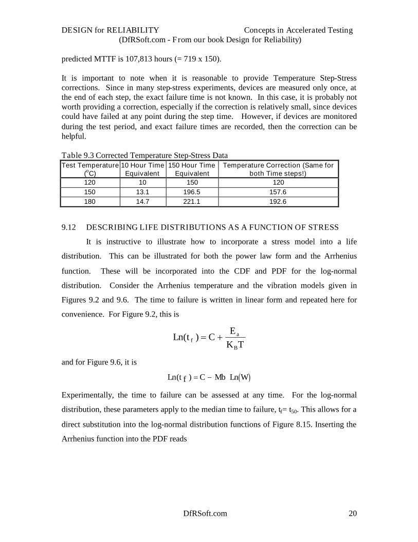
predicted MTTF is 107,813 hours (= 719 x 150).
It is important to note when it is reasonable to provide Temperature Step-Stresscorrections. Since in many step-stress experiments, devices are measured only once, atthe end of each step, the exact failure time is not known. In this case, it is probably notworth providing a correction, especially if the correction is relatively small, since devicescould have failed at any point during the step time. However, if devices are monitoredduring the test period, and exact failure times are recorded, then the correction can behelpful.
Table 9.3 Corrected Temperature Step-Stress DataTest Temperature
(oC)10 Hour Time
Equivalent150 Hour Time
EquivalentTemperature Correction (Same for
both Time steps!)120 10 150 120150 13.1 196.5 157.6180 14.7 221.1 192.6
9.12 DESCRIBING LIFE DISTRIBUTIONS AS A FUNCTION OF STRESS
It is instructive to illustrate how to incorporate a stress model into a life
distribution. This can be illustrated for both the power law form and the Arrhenius
function. These will be incorporated into the CDF and PDF for the log-normal
distribution. Consider the Arrhenius temperature and the vibration models given in
Figures 9.2 and 9.6. The time to failure is written in linear form and repeated here for
convenience. For Figure 9.2, this is
TKE
CtLnB
af )(
and for Figure 9.6, it is
Ln t f C Mb Ln W( )
Experimentally, the time to failure can be assessed at any time. For the log-normal
distribution, these parameters apply to the median time to failure, tf= t50. This allows for a
direct substitution into the log-normal distribution functions of Figure 8.15. Inserting the
Arrhenius function into the PDF reads
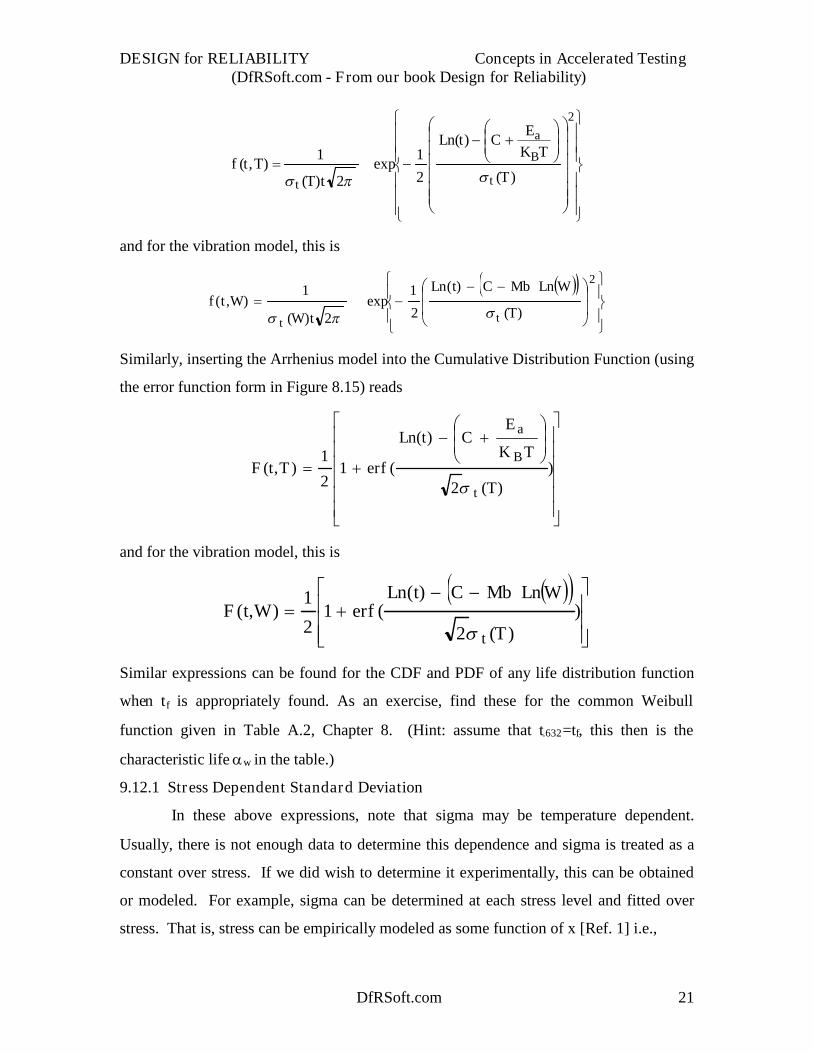
DESIGN for RELIABILITY Concepts in Accelerated Testing(DfRSoft.com - From our book Design for Reliability)
DfRSoft.com 21
2
)(
)(
21
exp2)(
1),(
T
TKE
CtLn
tTTtf
t
B
a
t
and for the vibration model, this is
2
)(
)(
2
1exp
2)(
1),(
T
WLnMbCtLn
tWWtf
tt
Similarly, inserting the Arrhenius model into the Cumulative Distribution Function (using
the error function form in Figure 8.15) reads
))(2
)(
(12
1),(
T
TK
ECtLn
erfTtFt
B
a
and for the vibration model, this is
)
)(2
)((1
2
1),(
T
WLnMbCtLnerfWtF
t
Similar expressions can be found for the CDF and PDF of any life distribution function
when tf is appropriately found. As an exercise, find these for the common Weibull
function given in Table A.2, Chapter 8. (Hint: assume that t.632=tf, this then is the
characteristic lifew in the table.)
9.12.1 Stress Dependent Standard Deviation
In these above expressions, note that sigma may be temperature dependent.
Usually, there is not enough data to determine this dependence and sigma is treated as a
constant over stress. If we did wish to determine it experimentally, this can be obtained
or modeled. For example, sigma can be determined at each stress level and fitted over
stress. That is, stress can be empirically modeled as some function of x [Ref. 1] i.e.,
DESIGN for RELIABILITY Concepts in Accelerated Testing(DfRSoft.com - From our book Design for Reliability)
DfRSoft.com 22
x)=f(+0x)
However, in an experiment, such as life tests over temperature stress, we already have a
failure time model and most likely the mean-time-to-failure has been fitted at each
temperature level. That is
Ln t f CEa
K BTC
EaKBT
( ) 50%50%
is experimentally estimated from the data. Here the constants have been identified from
fitting the mean-time-to-failure fit over stress. Additionally, we could also obtain a fit to
the data at the 16th percentile points in the distribution over stress denoted here as
Ln t f CEa
KBT( )16% 16%
16%
This gives a model for sigma based on the physical aging law and the data itself as
t T Ln t f Ln t f CEa
KBT( ) ( ) ( ) 16%
EXAMPLE 9.9 CDF as a Function of StressFor the vibration function, let C = -7.82, Mb = 4, and find F(t,W) for t = 10 years
and W = 0.0082 G2/Hz. Find F at 10 years. Use =2.2 for your estimate. If the stresslevel is reduced by a factor of 2, what is F?
SOLUTION: Inserting these values into the CDF above reads,
F t W erfLn
( , ) (ln( ) . .
.)
12
187600 7 82 4 0 0082
2 2 2
or
F erf erf( , . ) (
..
) (.
.) .87600 0 0082
12
10 01392 2 2
12
10 01392 2 2
0 497
Thus, at this stress level, 49.7% of the distribution is anticipated to have failed in 10years. (Note, in the above derivation, the error function values can be found from tablesor in Microsoft Excel type, =erf(0.00447) to obtain the above value.) If the stress level isreduced by a factor of 2, then W = 0.0041 G2/Hz. The anticipated percent failure at 10years is reduced to F(87600,0.0041) = 10.27%.
EXAMPLE 9.10 Relationship Between a Stress and Time Standard DeviationProvide a CDF model for the temperature stress distribution and find a
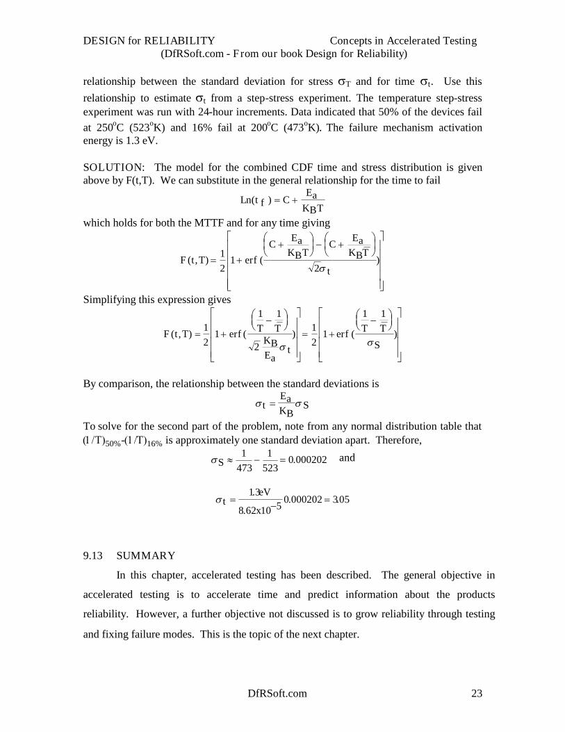
DESIGN for RELIABILITY Concepts in Accelerated Testing(DfRSoft.com - From our book Design for Reliability)
DfRSoft.com 23
relationship between the standard deviation for stress T and for time t. Use thisrelationship to estimate t from a step-stress experiment. The temperature step-stressexperiment was run with 24-hour increments. Data indicated that 50% of the devices failat 250oC (523oK) and 16% fail at 200oC (473oK)The failure mechanism activationenergy is 1.3 eV.
SOLUTION: The model for the combined CDF time and stress distribution is givenabove by F(t,T). We can substitute in the general relationship for the time to fail
Ln t f CEa
KBT( )
which holds for both the MTTF and for any time giving
F t T erf
CEa
KBTC
EaKBT
t( , ) ( )
12
12
Simplifying this expression gives
F t T erf T TKBEa
t
erf T T
S( , ) ( ) ( )
12
1
1 1
2
12
1
1 1
By comparison, the relationship between the standard deviations is
tEaKB
S
To solve for the second part of the problem, note from any normal distribution table that50%-16% is approximately one standard deviation apart. Therefore,
S 1
4731
5230 000202. and
teV
x
1 3
8 62 10 50 000202 3 05
.
.. .
9.13 SUMMARY
In this chapter, accelerated testing has been described. The general objective in
accelerated testing is to accelerate time and predict information about the products
reliability. However, a further objective not discussed is to grow reliability through testing
and fixing failure modes. This is the topic of the next chapter.
DESIGN for RELIABILITY Concepts in Accelerated Testing(DfRSoft.com - From our book Design for Reliability)
DfRSoft.com 24
9.14 REFERENCES
1. W. Nelson, Accelerated Testing, Wiley, New York, 1990.2. A.A. Feinberg, "The Reliability Physics of Thermodynamic Aging," in Recent
Advances in Life-Testing and Reliability, Edited by N. Balakrishnan, CRC Press, BocaRaton, FL.
3. D.S. Peck, “Comprehensive Model for Humidity Testing Correlation,” InternationalReliability Physics Symposium, 1986, pp. 44-50.
4. Tam, “Demonstrated Reliability of Plastic-encapsulated Microcircuits for MissileApplications,” IEEE Transactions on Reliability, Vol. 44, No. 1, 1995, pp. 8-13.
5. W. K. Denson, “A Reliability Model for Plastic Encapsulated Microcircuits,” Instituteof Environmental Sciences Proceedings, 42nd Annual Meeting, 1996, pp. 89-96.
6. J.R.Black, “Metallization Failures in Integrated Circuits,’ Technical Report, RADC-TR-68-43 (Oct. 1968).
7. J.R.Black, “Electromigration - A Brief Survey and Some Recent Results,” IEEETransactions on Electron Devices, Vol. ED-16 (No. 4), 1969, p. 338.