design, calibration and testing of a force balance for …
TRANSCRIPT
DESIGN, CALIBRATION AND TESTING OF A FORCE BALANCE FOR
A HYPERSONIC SHOCK TUNNEL
by
PRAVIN VADASSERY
Presented to the Faculty of the Graduate School of
The University of Texas at Arlington in Partial Fulfillment
of the Requirements
for the Degree of
MASTER OF SCIENCE IN AEROSPACE ENGINEERING
THE UNIVERSITY OF TEXAS AT ARLINGTON
MAY 2012

Copyright © by Pravin Vadassery 2012
All Rights Reserved

iii
ACKNOWLEDGEMENTS
Foremost, I am thankful to God for having blessed me throughout my life, without whom
nothing is possible. Next thanks go to Dr Frank Lu and Dr Don Wilson for their constant support
and for giving me the opportunity to work at the ARC (Aerodynamics Research Center). Again, I
am thankful to Dr Lu for his determination, enthusiasm and vast knowledge. His words of
encouragement, “Making mistakes is all part of the learning process”, helped me to overcome
the hardships during my research. A special thanks to Eric M Braun for his help, quick
suggestions and for always being around.
I acknowledge my fellow team mates in doing an excellent job of reconstructing the
UTA Hypersonic Shock Tunnel and getting it back on running condition. Special thanks go to
Tiago Rolim for his endless support and always assisting me in the times of repair, machining
and discussions. Thanks also to Derek Leamon, Nitesh K Manjunatha, Raheem Bello and
Dibesh Joshi.
I appreciate the work of all the technical staff involved in the Mechanical and Aerospace
Department. Special credit to Kermit Beird, Sam Williams and Rod Duke for fabrication of all
necessary parts and for sharing their practical knowledge. I sincerely thank everyone in the
ARC, also for making this place lively and ‘loud’.
Finally, I would like to thank my parents, family and friends for their patience and for
supporting me.
April 17, 2012

iv
ABSTRACT
DESIGN, CALIBRATION AND TESTING OF A FORCE BALANCE FOR
A HYPERSONIC SHOCK TUNNEL
Pravin Vadassery, M.S
The University of Texas at Arlington, 2012
Supervising Professor: Frank K. Lu
The forces acting on a flight vehicle are critical for determining its performance. Of
particular interest is the hypersonic regime. Force measurements are much more complex in
hypersonic flows, where those speeds are simulated in shock tunnels. A force balance for such
facilities contains sensitive gages that measure stress waves and ultimately determine the
different components of force acting on the model. An external force balance was designed and
fabricated for the UTA Hypersonic shock tunnel to measure drag at Mach 10. Static and
dynamic calibrations were performed to find the transfer function of the system. Forces were
recovered using a deconvolution procedure. To validate the force balance, experiments were
conducted on a blunt cone. The measured forces were compared to Newtonian theory.

v
TABLE OF CONTENTS
ACKNOWLEDGEMENTS ................................................................................................................ iii ABSTRACT ..................................................................................................................................... iv LIST OF ILLUSTRATIONS.............................................................................................................. vii LIST OF TABLES ............................................................................................................................. x Chapter Page
1. INTRODUCTION ……………………………………..………..…....................................... 1
1.1 Literature Survey .............................................................................................. 1
1.2 Force Measurement Techniques ..................................................................... 2
1.2.1 Internal Force Balance ..................................................................... 3 1.2.2 External Force Balance .................................................................... 3 1.2.3 Strain Gages .................................................................................... 4
1.2.4 Piezoelectric Film ............................................................................. 4
1.2.5 Accelerometer .................................................................................. 5
1.3 Convolution ...................................................................................................... 5
1.4 Objective of Research ...................................................................................... 7
2. FACILITY ........................................................................................................................ 8
2.1 UTA Hypersonic Shock Tunnel at the Aerodynamics Research Center .......................................................................................... 8
2.2 Reconstruction of the UTA Hypersonic Shock
Tunnel ........................................................................................................ 13
2.3 Diaphragm Test .............................................................................................. 13
3. DESIGN AND EXPERIMENTAL SETUP .................................................................... 15
3.1 Force Balance Design .................................................................................... 15
vi
3.1.1 Finite Element Analysis ................................................................. 18 3.1.2 Force Balance Construction .......................................................... 24
3.2 Calibration Technique .................................................................................... 29
3.2.1 Static Calibration ............................................................................ 29 3.2.2 Dynamic Calibration ...................................................................... 32
3.3 Shock Tunnel Testing ................................................................................... 42
4. RESULTS AND DISCUSSION .................................................................................... 43 4.1 Force Measurement Prediction ..................................................................... 43
4.1.1 Modified Newtonian Theory .......................................................... 43 4.1.2 Coefficient of Drag Calculation using Pitot Pressure .......................................................................... 46
4.2 Experimental Results ..................................................................................... 48
5. CONCLUSION AND FUTURE WORK ........................................................................ 53
5.1 Force Balance in the UTA Hypersonic Shock Tunnel ................................... 53
5.2 Future Work and Recommendations ............................................................ 55
APPENDIX
A. LIST OF DESIGN DRAWINGS ..................................................................................... 56
B. MATLAB PROGRAM FOR FORCE ESTIMATION ..................................................... 63
C. INSTRUMENTATION DETAILS .................................................................................. 67 REFERENCES ............................................................................................................................... 70 BIOGRAPHICAL INFORMATION .................................................................................................. 72
vii
LIST OF ILLUSTRATIONS
Figure Page 1.1 Linear input-output system (a) continuous (b) discrete .............................................................. 6 1.2 Convolution in time and frequency domain ................................................................................ 6 2.1 Schematic of the UTA Hypersonic Shock Tunnel ..................................................................... 9 2.2 Panorama view of the UTA Hypersonic Shock Tunnel .............................................................. 9 2.3 Schematic of the double diaphragm section ........................................................................... 10 2.4 Photograph of double diaphragm section ............................................................................... 10 2.5 Steel diaphragms (a) scored diaphragm (b) ruptured diaphragm after test ........................................................... 14 3.1 Different preliminary designs .................................................................................................... 17 3.2 Fabricated force balance .......................................................................................................... 18 3.3 Generated mesh of the force balance ...................................................................................... 19 3.4 FEA analysis settings ............................................................................................................... 20 3.5 Strain concentration in stress bars .......................................................................................... 20 3.6 Simulated input load of 350 N .................................................................................................. 21 3.7 Response to simulated impulse at (a) location1 (b) location2 ......................................................................................................... 22 3.8 (a) Simulated step load of 222.4 N (b) step response of location 2 ........................................ 22 3.9 Animated result of stress wave propagation ............................................................................ 23 3.10 Blunt cone model (a) side view (b) front view ........................................................................ 24 3.11 Hardened steel bolt hinge ..................................................................................................... 25 3.12 Installed model and balance in the test section .................................................................... 26 3.13 Attached strain gages ........................................................................................................... 27 3.14 Installed model and balance in the test section, front view .................................................... 28

viii
3.15 Schematic of static calibration procedure ............................................................................. 29 3.16 Static loading and unloading of force balance ...................................................................... 30 3.17 Average film output versus hammer force ............................................................................ 32 3.18 Schematic of a cut weight test .............................................................................................. 33 3.19 Vertical cut weight test .......................................................................................................... 33 3.20 Schematic of impulse hammer calibration ............................................................................ 34 3.21 Raw data of hammer impulse test .......................................................................................... 35 3.22 Sample hammer impulse ...................................................................................................... 35 3.23 Check signal for both raw and modified hammer pulse ........................................................ 36 3.24 Detail view of check signal with error bar ............................................................................... 37 3.25 Simulated unit step input ....................................................................................................... 37 3.26 Modified hammer signal ......................................................................................................... 38 3.27 Enlarged view of the modified hammer pulse ....................................................................... 38 3.28 Impulse response obtained from FFT and JMECG .............................................................. 39 3.29 Power spectral density plot of FRF ....................................................................................... 40 3.30 Enlarged power spectral density plot of FRF for first 12 kHz ................................................ 40 3.31 Enlarged phase spectrum of FRF ......................................................................................... 41 3.32 Spectrogram of the FRF ........................................................................................................ 41 4.1 Plot of (a) coefficient of drag (b) coefficient of lift .................................................................... 45 4.2 Coefficient of drag from recovered force (condition 1) ............................................................ 48 4.3 Recovered drag force and predicted force .............................................................................. 49 4.4 Raw pitot pressure signal ....................................................................................................... 49 4.5 Detailed view of the pitot pressure signal and drag ................................................................. 50 4.6 Coefficient of drag from recovered force (condition 2) ............................................................. 50 4.7 Recovered drag force .............................................................................................................. 51 4.8 Raw pitot pressure signal ........................................................................................................ 51
ix
4.9 Detailed view of the pitot pressure signal ................................................................................ 52 A.1 Force balance drawing ............................................................................................................ 57 A.2 Blunt cone model drawing ...................................................................................................... 58 A.3 PCB pressure transducer holder drawing ............................................................................... 59 A.4 Hinge joint part 1 drawing ....................................................................................................... 60 A.5 Hinge joint part 2 drawing ....................................................................................................... 61 A.6 Scoring pattern on steel diaphragm drawing .......................................................................... 62 C.1 Amplifier circuit diagram for piezoelectric film ......................................................................... 69
x
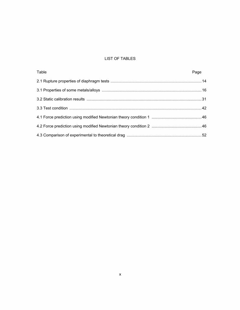
LIST OF TABLES
Table Page 2.1 Rupture properties of diaphragm tests .................................................................................... 14
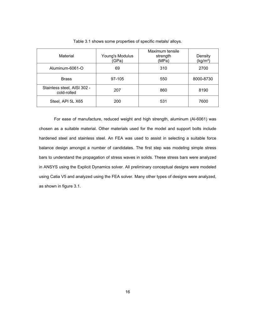
3.1 Properties of some metals/alloys ............................................................................................ 16
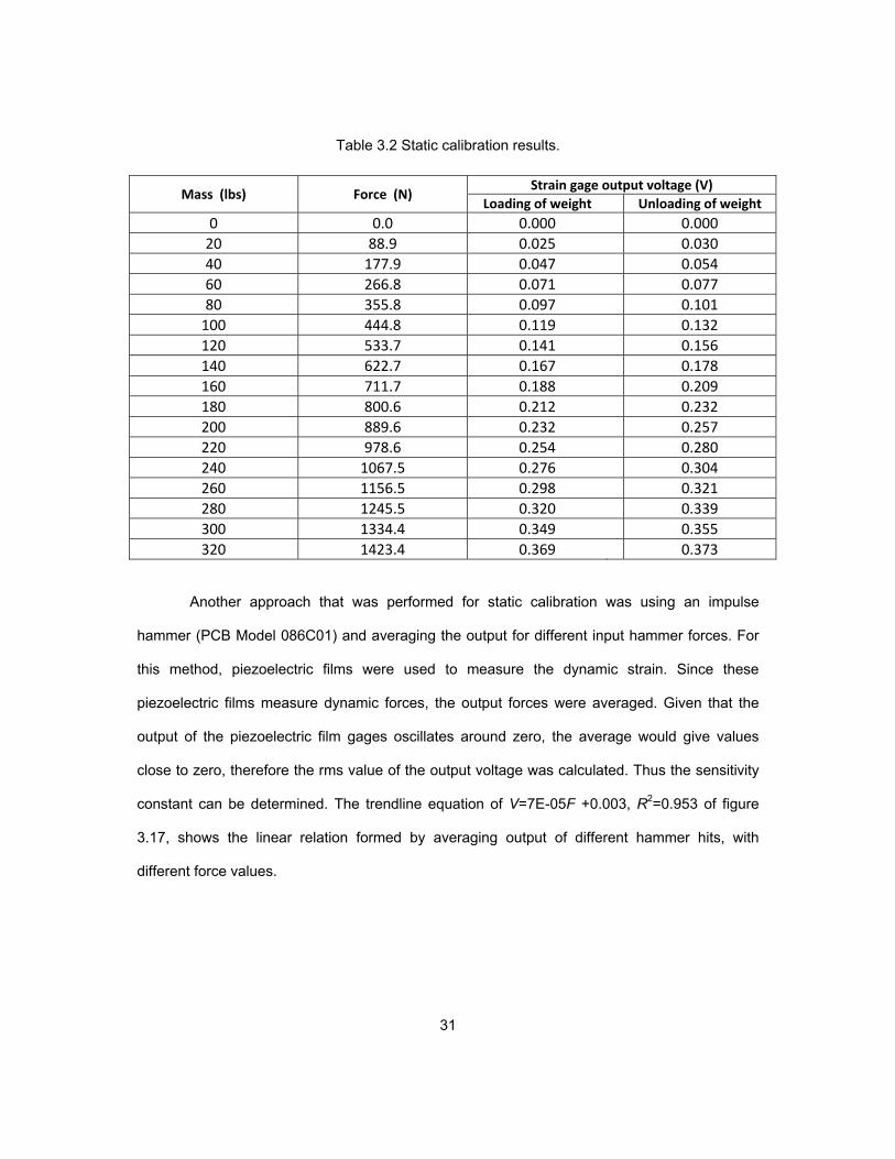
3.2 Static calibration results .......................................................................................................... 31
3.3 Test condition .......................................................................................................................... 42
4.1 Force prediction using modified Newtonian theory condition 1 .............................................. 46
4.2 Force prediction using modified Newtonian theory condition 2 .............................................. 46
4.3 Comparison of experimental to theoretical drag ..................................................................... 52
1
CHAPTER 1
INTRODUCTION
The forces acting on a flight vehicle are critical for determining its performance. Of
particular interest is the hypersonic regime. Research in hypersonics has led to successful tests
of scramjet (supersonic combustion ramjet) based vehicles, such as, NASA X-43A. In
hypersonic vehicle design, significance is laid on propulsion system integration, engine
performance, aerodynamics and thrust measurements. Specifically ground-based test facilities
have limited steady test time thus making force measurement complex in this very short
duration of time.
1.1 Literature Survey
Hypersonic wind tunnels have been in use since the 1950’s and have
developed into different types, namely, continuous and impulse types. Impulse facilities include
shock tubes, reflected shock tunnels and expansion tunnels. The basic principle of these
impulse facilities is to suddenly release a highly compressed gas in the so-called driver tube
through rupturing a diaphragm. The sudden release of the compressed gas propagates a shock
wave into a so-called driven tube filled with the test gas at low pressure. The shock
compresses and heats the test gas to the desired conditions, after which, it is expelled by a
nozzle to hypersonic conditions. For example, the T4 free piston shock tunnel at the University
of Queensland is an impulse-type facility that simulates hypersonic flows [1].

2
1.2 Force Measurement Technique
Throughout this thesis, force measurements refer to techniques for impulse
facilities unless noted otherwise. Force measurement is complicated in impulse facilities due to
the short test duration that will likely prevent the force balance from attaining a steady state.
This limitation of short test times in such facilities was overcome by applying the stress wave
force measurement technique (SWFM), proposed by Sanderson and Simmons [2]. Due to
impulsive aerodynamic loading, stress waves that are created, propagate and reflect through
the model and support structure, which are measured and analyzed by this method. Extension
of this work by Daniel and Mee [3] using finite element modeling led to the design of a three-
component force balance. The SWFM technique is based on the principle that, when stress
waves travels, no force equilibrium is reached in such a short duration of time so that the strain
histories are the crucial feature for developing force measurement techniques.
An investigation into internal and external force balances was undertaken by Robinson
et al. [4] which showed that a higher accuracy of the recovered force and moment loads was
attained using an external force balance. Also, for a blunt body, these authors found that the
interaction of external balance on the model forces was negligible when compared to that of an
internal balance. Some of the recent developments include comparing the experimental
measurements with CFD calculations by Boyce and Stumvoll [5], which showed good
agreement for a range of Mach numbers and test gases.
On the other hand, accelerometer-based force balance were used by Kulkarni and
Reddy [6] and Sahoo et al [7], which was a single-component accelerometer force balance. The
data were in accordance with modified Newtonian theory. Sahoo et al. [8], found that the drag
measured on a 30 degree semi-apex angle blunt cone model at Mach 5.75 with an accelerator-
based balance agreed closely to the SWFM technique.
3
1.2.1 Internal Force Balance
Internal force balances are defined as those that have the measuring instruments like
strain gages, accelerometers placed inside the model. The mounting system (sting) has to
adapt depending on the location of the force balance. Models are generally attached to a long
sting and placed in the test section of the tunnel. The geometry of the model has to
accommodate the sting. A common way to measure forces is by strain gages. Strain gages
work on the principle that when a load is applied, the stretching or deformation of the gage
causes a change in electrical resistance, details can be found in Section 1.2.3.
1.2.2 External Force Balance
External balances are those where the measuring instruments are located outside the
model but may be within the test section. The definition of external balances used to be
restricted those that are mounted outside the test section, which has been updated to balances
that are specifically external to the model, but which can be within the test section. The principle
of external balances is similar to that of internal balances but the difference is that the
measuring devices are placed on a supporting structure, such as a sting. The forces on the
model are transmitted as stress waves to the sting, which on deformation or bending creates
strain that is measured by the attached strain gages. Specifically for hypersonic shock tunnels,
external force balances that use stress wave propagation are named as Stress Wave Force
Balances (SWFB) [2].
During a run in an impulse facility, the sudden aerodynamic load initiates stress waves
in the model. The stress waves propagate and reflect between the model and the support
structure. A steady state of force equilibrium cannot be achieved between the model and the
support structure, since the duration of steady flow time is very minute. The SWFB concept
operates on the principle that no steady-state force equilibrium is achieved [9]. The force
balance forms a linear system, where the forces can be obtained by a deconvolution technique,
which is discussed further in a later chapter. A SWFB is suspended from the test section by

4
means of thin wires, with the strain gages mounted on the supporting sting. Different kinds of
materials have been used for SWFB construction such as brass, aluminum or steel.
1.2.3 Strain Gages
Strain gages are sensors that are used to measure strain or deformation. Strain gages
work by the principle that a strain in a metal or semi-conductor causes a change in resistance,
which when measured can be related to the strain. There are different types of strain gages,
namely, metallic foil gages and semiconductor strain gages, which can be either piezo-resistive
or piezoelectric. All resistance-based strain gages require an excitation voltage. A Wheatstone
bridge arrangement increases the sensitivity of the strain gage, thus allowing small changes in
strain to be measured.
1.2.4 Piezoelectric Film
Piezoelectric film gages are a type of transducer for measuring dynamic strain and are
used in high-frequency applications .Some of the features of piezo film are its flexibility, varying
thickness, lightweight and easy application. These gages have a large frequency range of up to
the order of 1 GHz. Some other properties include its dynamic range, high mechanical strength,
and temperature and humidity stability. Piezoelectric film can be adapted to various shapes and
can be bonded with commercial adhesives. Another feature is high voltage output, that can be
as high as 10 times higher than normal strain gages. Some disadvantages of piezoelectric films
are that they are sensitive to electromagnetic radiation, in such cases shielding becomes
important to avoid any kind of interference and ensuring a good signal-to-noise ratio.
Piezoelectric film gages do not require an external power source or excitation voltage.
Marineau [11] showed that a piezoelectric force balance has a higher frequency response than
a strain gage force balance. Both balances showed comparable levels of accuracy. The
piezoelectric balance shows a 350% increase in frequency response and 400% increase in
sensitivity.
5
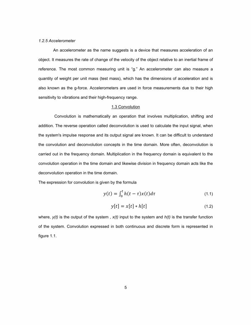
1.2.5 Accelerometer
An accelerometer as the name suggests is a device that measures acceleration of an
object. It measures the rate of change of the velocity of the object relative to an inertial frame of
reference. The most common measuring unit is “g.” An accelerometer can also measure a
quantity of weight per unit mass (test mass), which has the dimensions of acceleration and is
also known as the g-force. Accelerometers are used in force measurements due to their high
sensitivity to vibrations and their high-frequency range.
1.3 Convolution
Convolution is mathematically an operation that involves multiplication, shifting and
addition. The reverse operation called deconvolution is used to calculate the input signal, when
the system's impulse response and its output signal are known. It can be difficult to understand
the convolution and deconvolution concepts in the time domain. More often, deconvolution is
carried out in the frequency domain. Multiplication in the frequency domain is equivalent to the
convolution operation in the time domain and likewise division in frequency domain acts like the
deconvolution operation in the time domain.
The expression for convolution is given by the formula
(1.1)
∗ (1.2)
where, y(t) is the output of the system , x(t) input to the system and h(t) is the transfer function
of the system. Convolution expressed in both continuous and discrete form is represented in
figure 1.1.

6
Figure 1.1 A linear input-output system a) continuous, b) discrete.
Due to the large number of multiplications and additions that must be performed in the
convolution algorithm, it can be inefficient when a large amount of data needs to be processed.
As stated above, the convolution could be made easy by multiplication in the frequency domain
via Fourier and inverse Fourier transforms, represented in equation (1.3).
(1.3)
A block diagram showing the input-output relationship in the time and frequency
domains is depicted in Fig. 1.2. Fourier transform is used to change a signal from time domain
to frequency domain. The reverse is done by inverse Fourier transform. The frequency
response is a complex function of frequency that can be expressed by a magnitude and a
phase spectrum.
Figure 1.2 The relationship of convolution in time domain and in the frequency domain [12].
Linear system h(t)
x(t) y(t)
x(n) y(n)Linear system h(n)
(a)
(b)
h(t)x(t) y(t)
IFT FT
IFT FT
h(f)x(f) y(f)
Time Domain
Frequency Domain
7
1.4 Objective of Research
The goal of this research is to design, calibrate and test a simple force balance system
that is capable of measuring drag on various models. As the test time is of very short duration,
force measurement becomes a challenge. To design this force balance system, an approach is
utilized to model the response of the balance using FEA. ANSYS Explicit Dynamics solver is
used for the dynamic analysis. Piezoelectric films were used to measure stress waves due to
aerodynamic loading. Deconvolution was used to determine the system transfer function and to
recover the force. The drag on a spherically blunted cone was measured and the drag
coefficient was compared with that obtained from modified Newtonian theory. Future efforts
would consist of extension of the force balance to measure other components of force, such as
lift and pitching moment. Force measurement on other models, such as conical model, inlets
and scramjet vehicles would be included.
8
CHAPTER 2
FACILITY
2.1 UTA Hypersonic Shock Tunnel at the Aerodynamics Research Center
The Hypersonic Shock Tunnel at the UTA Aerodynamics Research Center is a reflected
type. It was designed and built in the late 1980’s [13]. The main components of the hypersonic
shock tunnel include the driver section, driven tubes, nozzle, test section, diffuser and dump
tank, which are shown in figure 2.1.
This facility is able to simulate high Mach numbers and high enthalpy flows. The main
parts of this shock tunnel are:
Driver tube
Diaphragm section
Driven tubes
Nozzle
Test section
The shock tube is fabricated in four sections for ease of transportation, installation and
maintenance [14]. The driver tube is a single section which is designed for a maximum
operating driver pressure of 41.4 MPa (6000 psi) and hydrostatically tested to 62.1 MPa (9000
psi). The driver tube is 3 m (10 ft.) long with an internal diameter of 15.24 cm (6 in.) and a wall
thickness of 2.54 cm (1.0 in.). One end is closed off with a hemispherical end cap.

9
FFigure 2.1 Schem
Figure 2.2 Pan
matic of the UTA H
norama photogra
Hypersonic Shoc
aph of the UTA Hy
k Tunnel and its d
ypersonic Shock
dimensions
Tunnel

The o
drive
O-rin
seal
beca
flang
Figur
Figurdrive
other end has
er tube to be b
ng grooves m
[15].
The doub
use it is used
ges. Steel bolt
re 2.3 Schem
re 2.4 Photoen section (lef
s a 48.26 cm
bolted to the d
achined in th
ble diaphragm
d to hold two
ts of 2 in. diam
matic of the do
ograph of theft). The steel p
(19 in.) diam
diaphragm se
em to accom
m section se
diaphragms.
meter are use
ouble diaphrag
e double diappipe is used t
10
meter 11.43 cm
ection and the
mmodate two O
eparates the
This section
ed to bolt the
gm section be
phragm sectito pressurize
m (4.5 in.) thic
e driven sectio
O-rings to en
driver from
has the sam
flanges toget
etween the dr
on (middle), the double di
ck flange, wh
on [15]. The fl
nsure a tight,
the driven tu
me dimension
ther.
river and drive
driver sectioiaphragm sec
ich allows the
lange has two
high-pressure
ube, so-called
as that of the
en tube [15].
on (right) andction.
e
o
e
d
e
d
11
The driven tube is constructed in three segments of 2.74 m (9 ft) length each. The three
segments are connected to each other with a flange at each end identical to the one on the
driver section. The internal diameter is the same as the driver tube. Two O-rings are located
between each connection to provide a good high-pressure seal.
The expansion nozzle was developed by LTV Aerospace and Defense Company,
presently a part of Lockheed Martin Missiles and Fire Control. It was part of an arc-driven
hypervelocity wind tunnel facility and was subsequently donated to UTA. The end of the driven
tube has a special coupling for the nozzle insert and secondary diaphragm. The coupling
consists of several parts that form a locking system for the throat insert. The nozzle has
interchangeable throat inserts to provide a discrete test section Mach numbers of 5 to 16. The
nozzle has a length of 2.57 m (101 in), with an exit diameter of 33.6 cm (13.25 in) at the test
section [15].
The test section has a dimension of 53.6 cm (21.1 in.) in length and 44 cm (17.5 in.) in
diameter. It has circular access windows of 23 cm (9 in.) diameter facing each other on either
side. These two ports can be used as mounting ports or for optical windows [10]. The rear of
the test section has a conical converging section which leads into the diffuser. The dimensions
of the converging section are 38.1 cm (15 in) in diameter within the test section and it contracts
to a diameter of 31 cm (12.2 in) to the entrance of the diffuser. The flow is captured by the
converging section and generates the first shock wave necessary to slow the flow down in the
diffuser [15].
The dump tank is located outside the building and has a volume of 4.25 m3 (150 ft3).
The vacuum system vacuums the shock tunnel from the tank to the secondary diaphragm. A
35.6 cm (14 in) vacuum pipe is connected directly from the dump tank by a flange joint with a
double O-ring seal. A smaller 7.62 cm (3 in) diameter piping is used for connecting the vacuum
pump to the vacuum tank.
12
A high-pressure system is used to pressurize the driver tube. Another lower pressure
system is used to operate the remote control valves and the booster pump (Haskel model-
55696) on the high-pressure system. The high-pressure system consists of a 5-stage
compressor and a booster pump. The 5-stage compressor (Clark Model CMB-6) which is
located in the adjacent compressor building can provide dry air at up to 14.5 MPa (2100 psi).
The booster pump (Haskel Model 55696) is a two-stage booster pump which is used to attain
pressures of up to 41.4 MPa (6000 psi) in the driver tube. The Haskel pump uses dried, filtered
compressed air from the main compressor or helium supplied from 2200 psi bottles. The
pressurized gas is stored in a one meter diameter spherical storage tank which can hold
pressures up to 41.4 MPa (6000 psi).
The low pressure is generated by another compressor (Kellogg American inc. model-
DB462-C) which supplies dry air at 1.2 MPa (175 psi). Regulators are used to reduce the
pressure to 689.5 kPa (100 psi), which is needed for the booster pump operation. The low-
pressure compressed air (175 psi) is used by both the vacuum pump isolation valves and the
booster pump in the high-pressure system.
A secondary diaphragm separates the driven section from the test section. Both the
driven section and the test section including the nozzle have their own vacuum pumps. The
driven tube is vacuumed by a vacuum pump (Sargent-Welch Model 1376). This pump has a
free-air displacement of 300 liters per minute and is able of pumping down to 0.001 mmHg. The
test section is vacuumed by another vacuum pump (Sargent-Welch Model 1396) which is
connected to the dump tank. This pump is capable of a free-air displacement of 2800 liters per
minute and is able of achieving low pressures of up to 0.0001 mmHg. Vacuum is measured in
both the driven tube and the dump tank by a pressure gauge (MKS Baratron Type 127A). The
gauge has a full-scale range of 1000 mmHg and an accuracy of 0.1 mmHg.

13
2.2 Reconstruction of the UTA Hypersonic Shock Tunnel
The hypersonic shock tunnel had not been in use for many years and had been
disassembled for a long time due to other research activities. Reconstruction was needed and
began in 2010, where some of the parts had to be repaired or replaced with redesigned parts.
The hypersonic shock tunnel began full operation by mid 2011.
The first steps involved were setting up the driven tube sections which included removal
of corrosion and cleaning the inner tube. The diaphragm section was attached back to the driver
segment. For obtaining a good vacuum, the system had to be rechecked to ensure good seal. A
schedule 40-steel pipe of 76 mm (3 in.) internal diameter and 2.13 m (7 ft.) length had to be
replaced and customized for convenient attachment to the external dump tank. Safety valves
from the dump tank had to be replaced. Due to corrosion of the inner surface of the tank, it was
cleaned and treated with Enrust™ to prevent further occurrence. Some components had to be
refabricated or redesigned. The throat locking mechanism for the nozzle inserts had to be
fabricated in 4340-stainless steel. A diffuser section was designed for convenient sting
installation. This section has five ports used for model mounting and instrumentation purposes.
2.3 Diaphragm Test
As mentioned before, the driver and driven tube are separated by double diaphragms
made of 1008 steel (10/12gage, 0.03 in. thickness). New thickness tests had to be conducted
for higher pressure in the range of 20~30MPa (3000~4500 psi). Thickness and scoring play
important roles for achieving proper rupture. In some tests, the petals were torn off, which are
undesirable. These steel diaphragms must be scored with a cross pattern on each run, for
perfect rupture. Several tests were conducted on the scoring depth and thickness of the plate,
to improve the quality of the rupture and to contain the needed pressure. The tests ensured a
clean rupture and minimal petal fragmentation. Detailed drawing is given in appendix A. The
special cross pattern, known as a cross potent in heraldry was made [15] with a CNC machine
for quick manufacturing and reduced cost. Moreover, CNC machining helps in maintaining
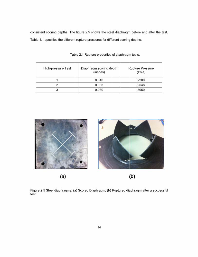
cons
Table
Figurtest.
sistent scoring
e 1.1 specifie
re 2.5 Steel d
High-pre
g depths. The
es the differen
Ta
diaphragms, (
essure Test
1
2
3
e figure 2.5 s
nt rupture pres
ble 2.1 Ruptu
a) Scored Dia
Diaphrag
14
shows the ste
ssures for diff
ure properties
aphragm, (b)
gm scoring de(inches)
0.040
0.035
0.030
eel diaphragm
ferent scoring
s of diaphragm
Ruptured dia
epth R
m before and
g depths.
m tests.
aphragm after
Rupture Press
(Psia)
2200
2548
3050
after the test
r a successfu
sure
t.
ul

15
CHAPTER 3
DESIGN AND EXPERIMENTAL SETUP
3.1 Force Balance Design
An investigation was conducted by Robinson et al. [4] on both internal and external
balances to measure forces and moments using FEA (finite element analysis). Their analysis
showed that greater accuracy of the recovered forces and moments could be obtained with the
external force balance design. For the present work, the design of an external force balance
(stress wave force balance) was investigated. This balance has the ability of mounting a variety
of models. Some of the conceptual design requirements included:
1. Size constraint.
2. Strength of Balance and other components.
3. Model and support attachment
4. Strain gage and transducer placement.
6. Calibration ease
7. Machining simplicity
The force balance can only be accommodated in the limited room given by the
dimension of the test section, including the model. The design should be able to adapt to the
test section of the UTA Hypersonic Shock Tunnel, which has a dimension of 53.6 cm (21.1 in.)
in length and 44 cm (17.5 in.) in diameter. The strength of the balance is important in deciding
on the type of material. Different type of metals including steel, stainless steel, brass and
aluminum were investigated.
16
Table 3.1 shows some properties of specific metals/ alloys.
Material Young's Modulus (GPa)
Maximum tensile strength (MPa)
Density (kg/m³)
Aluminum-6061-O 69 310 2700
Brass 97-105 550 8000-8730
Stainless steel, AISI 302 - cold-rolled
207 860 8190
Steel, API 5L X65 200 531 7600
For ease of manufacture, reduced weight and high strength, aluminum (Al-6061) was
chosen as a suitable material. Other materials used for the model and support bolts include
hardened steel and stainless steel. An FEA was used to assist in selecting a suitable force
balance design amongst a number of candidates. The first step was modeling simple stress
bars to understand the propagation of stress waves in solids. These stress bars were analyzed
in ANSYS using the Explicit Dynamics solver. All preliminary conceptual designs were modeled
using Catia V5 and analyzed using the FEA solver. Many other types of designs were analyzed,
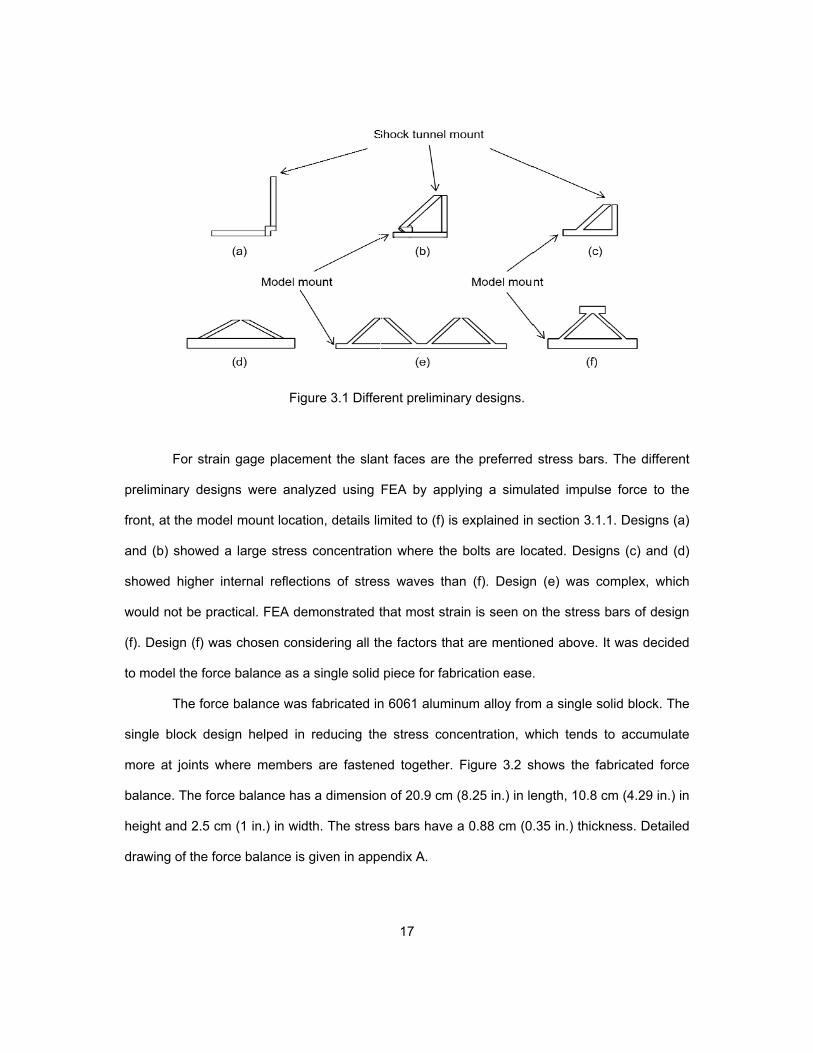
as shown in figure 3.1.
prelim
front
and
show
woul
(f). D
to mo
singl
more
balan
heigh
draw
For strain
minary desig
, at the mode
(b) showed a
wed higher in
d not be prac
Design (f) was
odel the force
The force
e block desig
e at joints wh
nce. The forc
ht and 2.5 cm
wing of the forc
Fig
n gage placem
ns were ana
el mount locat
a large stress
nternal reflect
ctical. FEA de
s chosen con
e balance as a
e balance was
gn helped in
here member
e balance ha
m (1 in.) in wid
ce balance is
gure 3.1 Diffe
ment the slan
alyzed using
tion, details li
s concentratio
tions of stres
emonstrated t
nsidering all th
a single solid
s fabricated in
reducing the
rs are fasten
s a dimension
dth. The stres
s given in app
17
rent prelimina
nt faces are t
FEA by appl
mited to (f) is
on where the
ss waves tha
that most stra
he factors tha
piece for fab
n 6061 alumin
e stress con
ed together.
n of 20.9 cm
ss bars have
endix A.
ary designs.
the preferred
lying a simul
s explained in
e bolts are loc
an (f). Design
ain is seen on
at are mentio
rication ease
num alloy from
centration, w
Figure 3.2 s
(8.25 in.) in le
a 0.88 cm (0
stress bars.
lated impulse
n section 3.1.1
cated. Design
n (e) was co
n the stress b
ned above. It
.
m a single so
which tends to
shows the fab
ength, 10.8 c
.35 in.) thickn
The differen
e force to the
1. Designs (a
ns (c) and (d
omplex, which
bars of design
t was decided
olid block. The
o accumulate
bricated force
m (4.29 in.) in
ness. Detailed
nt
e
)
)
h
n
d
e
e
e
n
d

3.1.1
defor
The A
unde
used
equa
wherm isc isk isu isp(t) is
1 Finite Eleme
Finite elem
rmations, was
ANSYS Expli
er a time-vary
d for impact
ation of motion
re s the mass ofs the dampings the stiffnesss the displaces the vector o
Figure 3.2 F
ent Analysis
ment analysis
s used to ve
cit Dynamics
ying load typic
analysis, sho
n in structura
f the system, g coefficient , s constant , ements vectorof the time-va
abricated forc
s which helps
rify the stress
solver is use
cally with dura
ock propagat
l dynamic ana
r rying load.
18
ce balance (6
s to determine
s concentrati
ed to understa
ations of less
tion and stre
alysis is given
6061- aluminu
e stress distri
on and respo
and the dynam
than 1 secon
ess wave pro
n by,
um alloy)
ibution, displa
onse of the f
mic response
nd. This solve
opagation. Th
acements and
force balance
of a structure
er can also be
he differentia
(3.1
d
e.
e
e
al
)

19
At each point in time, the vectors of displacement , velocity and acceleration are
of particular interest to determine stress concentration of the balance and understand its
dynamic response.
A mesh was generated using the explicit meshing feature. Tetrahedral elements were
used to mesh the force balance. A total number of 34088 elements was used in the simulation.
A uniform mesh was generated with default size elements to respond to high frequencies of the
stress wave. Mesh refinement was used for computational efficiency, by maintaining larger
elements to insignificant areas and increasing relevance to areas of higher stress concentration.
Care was taken in this process, as a coarse mesh was not able to transmit high-frequency
information to the finer mesh [1]. Damping was not used in the simulation, so as to acquire high
frequency stress waves. For computational ease, the balance was analyzed without the other
small components. Figure 3.3 shows the mesh of the force balance.
Figure 3.3 Generated mesh of the force balance using explicit dynamics.
The force balance was modeled as a rigid body, the top surface, a fixed support and
the simulated force was applied from the front face, which is shown in figure 3.4. The time step

is co
solut
ontrolled by th
tion time step
Figu
Fig
he smallest e
was 0.085 µs
ure 3.4. Anal
gure 3.5 Strai
element size,
s.
ysis settings,
n concentratio
20
which is use
force is appl
on in stress b
ed to progress
ied from the f
bars of the for
s the solution
front surface.
rce balance.
n in time. The
e
21
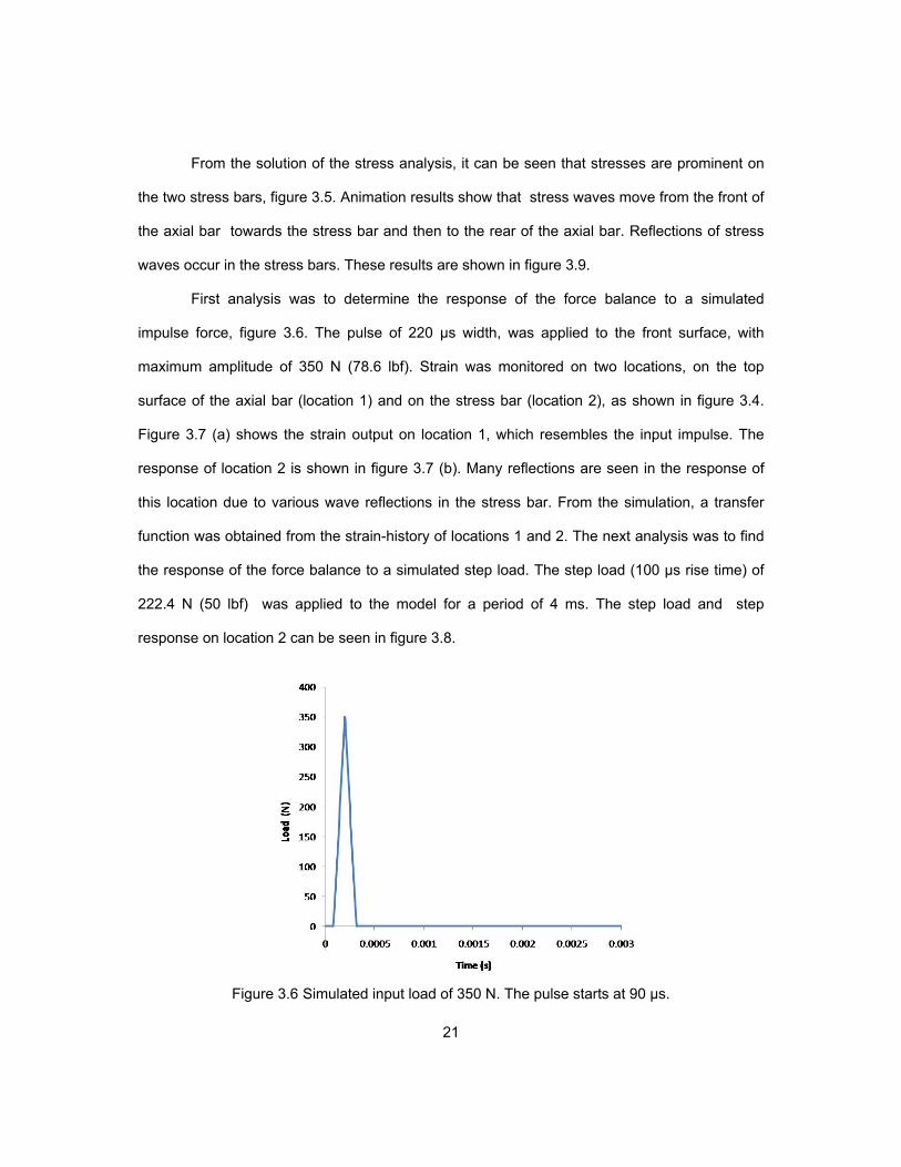
From the solution of the stress analysis, it can be seen that stresses are prominent on
the two stress bars, figure 3.5. Animation results show that stress waves move from the front of
the axial bar towards the stress bar and then to the rear of the axial bar. Reflections of stress
waves occur in the stress bars. These results are shown in figure 3.9.
First analysis was to determine the response of the force balance to a simulated
impulse force, figure 3.6. The pulse of 220 µs width, was applied to the front surface, with
maximum amplitude of 350 N (78.6 lbf). Strain was monitored on two locations, on the top
surface of the axial bar (location 1) and on the stress bar (location 2), as shown in figure 3.4.
Figure 3.7 (a) shows the strain output on location 1, which resembles the input impulse. The
response of location 2 is shown in figure 3.7 (b). Many reflections are seen in the response of
this location due to various wave reflections in the stress bar. From the simulation, a transfer
function was obtained from the strain-history of locations 1 and 2. The next analysis was to find
the response of the force balance to a simulated step load. The step load (100 µs rise time) of
222.4 N (50 lbf) was applied to the model for a period of 4 ms. The step load and step
response on location 2 can be seen in figure 3.8.
Figure 3.6 Simulated input load of 350 N. The pulse starts at 90 µs.
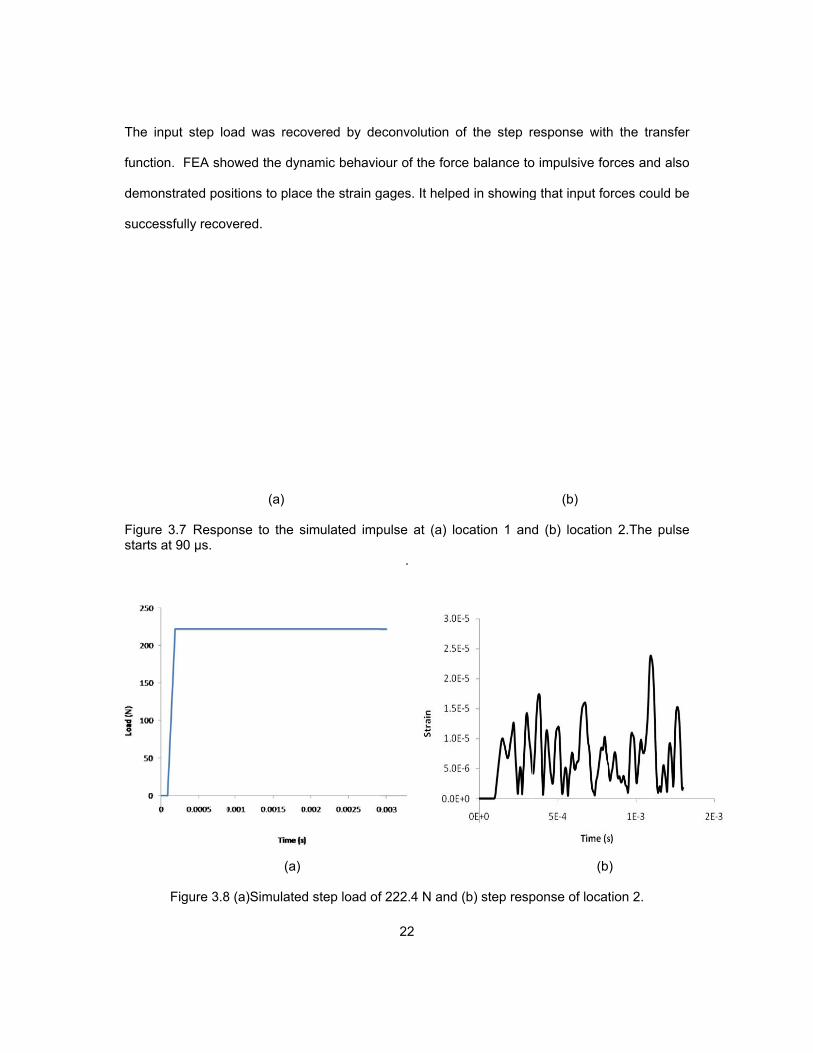
The
funct
demo
succ
Figurstarts
input step lo
tion. FEA sho
onstrated pos
essfully recov
re 3.7 Respos at 90 µs.
Figure 3.8
oad was reco
owed the dyn
sitions to plac
vered.
(a)
onse to the s
(a)
8 (a)Simulated
overed by de
namic behavio
ce the strain g
simulated imp
d step load of
22
econvolution o
our of the forc
gages. It helpe
pulse at (a) lo
.
f 222.4 N and
of the step r
ce balance to
ed in showing
ocation 1 and
d (b) step resp
response with
o impulsive fo
g that input fo
(b)
d (b) location
(b
ponse of locat
h the transfe
orces and also
orces could be
n 2.The pulse
)
tion 2.
er
o
e
e

Figure 3.9 AAnimated result shows the
23
e stress wave propagation in the force bbalance.
3.1.2
attac
conv
botto
draw
and
mode
degre
show
mode
was
throu
reces
press
2 Force Balan
A 12.7 m
chment. Two
veniently into
om for attachm
wing given in a
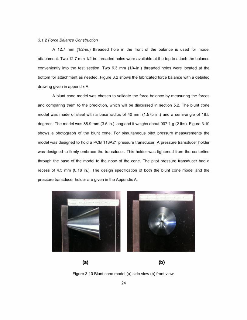
A blunt co
comparing th
el was made
ees. The mod
ws a photogr
el was design
designed to
ugh the base
ss of 4.5 mm
sure transduc
nce Construct
mm (1/2-in.)
12.7 mm 1/2-
the test sec
ment as need
appendix A.
one model wa
hem to the pr
e of steel with
del was 88.9
raph of the b
ned to hold a
firmly embrac
of the mode
m (0.18 in.). T
cer holder are
Figure 3.10
tion
threaded ho
-in. threaded
ction. Two 6.3
ded. Figure 3.
as chosen to
rediction, whi
h a base rad
mm (3.5 in.)
blunt cone. F
PCB 113A21
ce the transd
el to the nose
The design s
e given in the
0 Blunt cone m
24
le in the fro
holes were a
3 mm (1/4-in
.2 shows the
o validate the
ch will be dis
ius of 40 mm
long and it we
For simultane
1 pressure tra
ducer. This ho
e of the cone
specification
Appendix A.
model (a) side
ont of the ba
vailable at the
n.) threaded
fabricated for
force balanc
scussed in se
m (1.575 in.)
eighs about 9
eous pitot pre
ansducer. A p
older was tigh
e. The pitot p
of both the b
e view (b) fron
alance is use
e top to attac
holes were lo
rce balance w
ce by measur
ection 5.2. Th
and a semi-
907.1 g (2 lbs
essure meas
pressure tran
htened from
pressure tran
blunt cone m
nt view.
ed for mode
ch the balance
ocated at the
with a detailed
ing the forces
he blunt cone
-angle of 18.5
s). Figure 3.10
urements the
sducer holde
the centerline
sducer had a
model and the
el
e
e
d
s
e
5
0
e
er
e
a
e
25
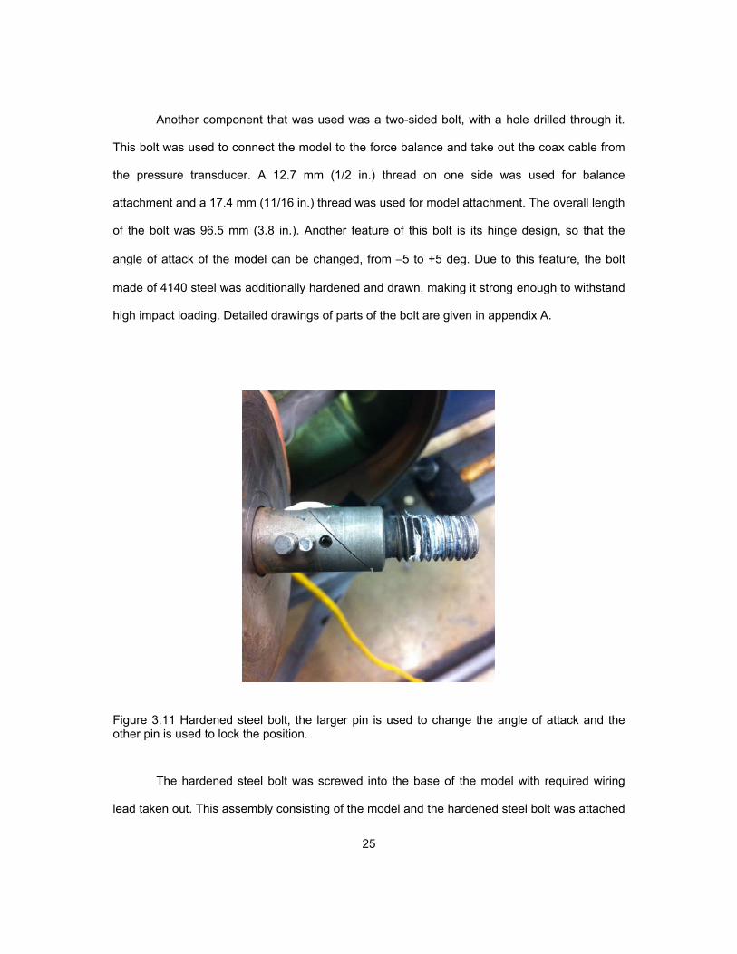
Another component that was used was a two-sided bolt, with a hole drilled through it.
This bolt was used to connect the model to the force balance and take out the coax cable from
the pressure transducer. A 12.7 mm (1/2 in.) thread on one side was used for balance
attachment and a 17.4 mm (11/16 in.) thread was used for model attachment. The overall length
of the bolt was 96.5 mm (3.8 in.). Another feature of this bolt is its hinge design, so that the
angle of attack of the model can be changed, from 5 to +5 deg. Due to this feature, the bolt
made of 4140 steel was additionally hardened and drawn, making it strong enough to withstand
high impact loading. Detailed drawings of parts of the bolt are given in appendix A.
Figure 3.11 Hardened steel bolt, the larger pin is used to change the angle of attack and the other pin is used to lock the position.
The hardened steel bolt was screwed into the base of the model with required wiring
lead taken out. This assembly consisting of the model and the hardened steel bolt was attached
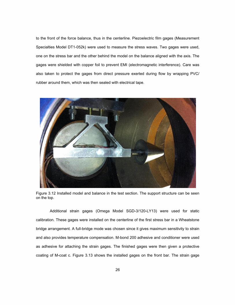
26
to the front of the force balance, thus in the centerline. Piezoelectric film gages (Measurement
Specialties Model DT1-052k) were used to measure the stress waves. Two gages were used,
one on the stress bar and the other behind the model on the balance aligned with the axis. The
gages were shielded with copper foil to prevent EMI (electromagnetic interference). Care was
also taken to protect the gages from direct pressure exerted during flow by wrapping PVC/
rubber around them, which was then sealed with electrical tape.
Figure 3.12 Installed model and balance in the test section. The support structure can be seen on the top.
Additional strain gages (Omega Model SGD-3/120-LY13) were used for static
calibration. These gages were installed on the centerline of the first stress bar in a Wheatstone
bridge arrangement. A full-bridge mode was chosen since it gives maximum sensitivity to strain
and also provides temperature compensation. M-bond 200 adhesive and conditioner were used
as adhesive for attaching the strain gages. The finished gages were then given a protective
coating of M-coat c. Figure 3.13 shows the installed gages on the front bar. The strain gage
27
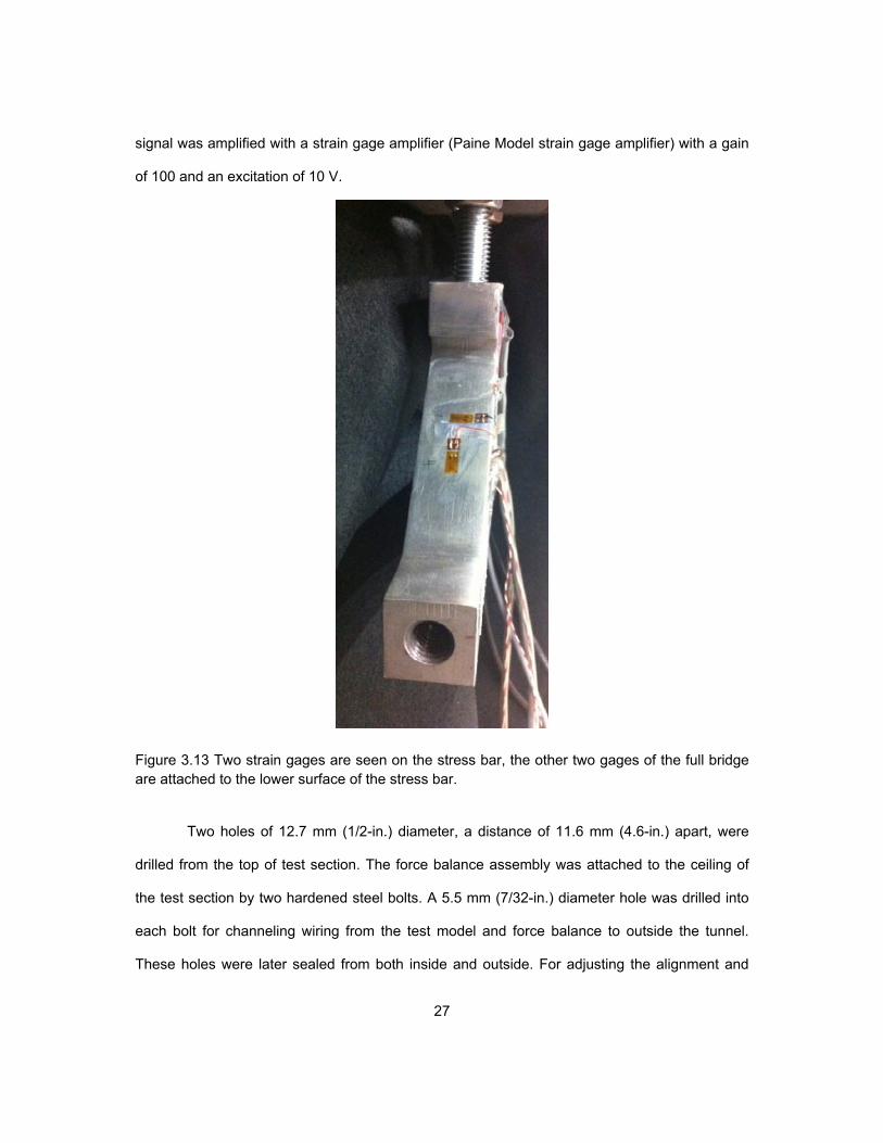
signal was amplified with a strain gage amplifier (Paine Model strain gage amplifier) with a gain
of 100 and an excitation of 10 V.
Figure 3.13 Two strain gages are seen on the stress bar, the other two gages of the full bridge are attached to the lower surface of the stress bar.
Two holes of 12.7 mm (1/2-in.) diameter, a distance of 11.6 mm (4.6-in.) apart, were
drilled from the top of test section. The force balance assembly was attached to the ceiling of
the test section by two hardened steel bolts. A 5.5 mm (7/32-in.) diameter hole was drilled into
each bolt for channeling wiring from the test model and force balance to outside the tunnel.
These holes were later sealed from both inside and outside. For adjusting the alignment and
28
height of the force balance an aluminum block of dimensions 2.5 cm × 2.5 cm × 15.2 cm (1 in. ×
1 in. × 6 in.) was installed between the balance and the ceiling. The model-balance assembly
was attached to the aluminum block by two 12.7 mm (1/2-in.) steel bolts. Steel washers and
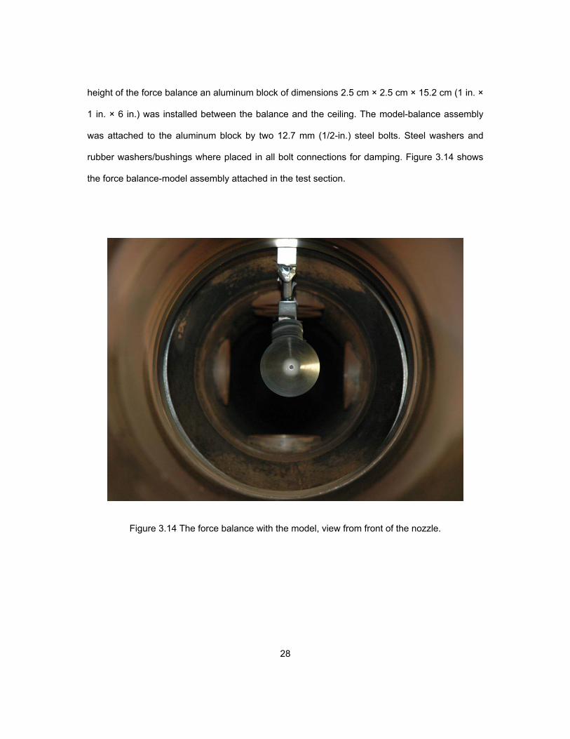
rubber washers/bushings where placed in all bolt connections for damping. Figure 3.14 shows
the force balance-model assembly attached in the test section.
Figure 3.14 The force balance with the model, view from front of the nozzle.
29
3.2 Calibration Techniques
3.2.1 Static Calibration
Static calibration is done by loading the force balance system with known weights and
measuring the output for each increasing load. After loading the balance unloading is performed
in like manner. This procedure helps to characterize the linearity and the possibility of hysteresis
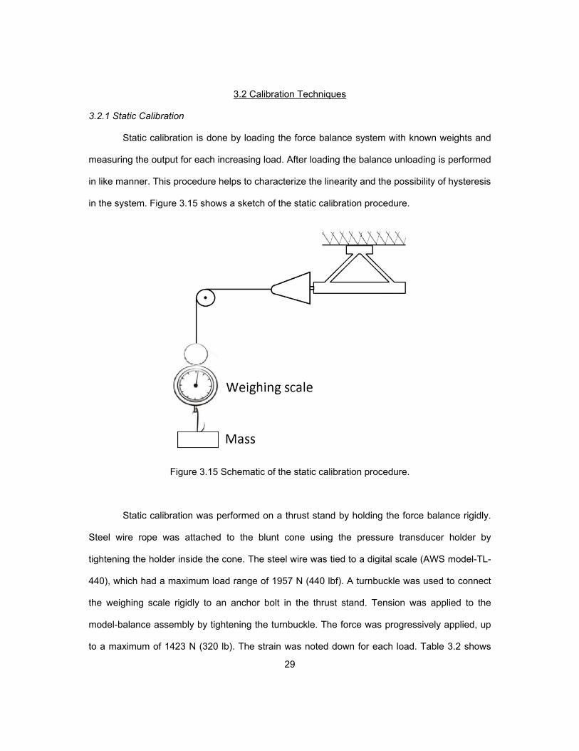
in the system. Figure 3.15 shows a sketch of the static calibration procedure.
Figure 3.15 Schematic of the static calibration procedure.
Static calibration was performed on a thrust stand by holding the force balance rigidly.
Steel wire rope was attached to the blunt cone using the pressure transducer holder by
tightening the holder inside the cone. The steel wire was tied to a digital scale (AWS model-TL-
440), which had a maximum load range of 1957 N (440 lbf). A turnbuckle was used to connect
the weighing scale rigidly to an anchor bolt in the thrust stand. Tension was applied to the
model-balance assembly by tightening the turnbuckle. The force was progressively applied, up
to a maximum of 1423 N (320 lb). The strain was noted down for each load. Table 3.2 shows
30
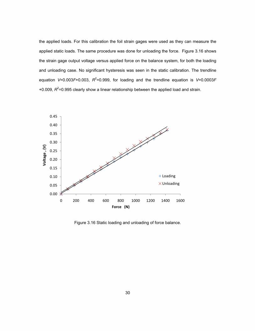
the applied loads. For this calibration the foil strain gages were used as they can measure the
applied static loads. The same procedure was done for unloading the force. Figure 3.16 shows
the strain gage output voltage versus applied force on the balance system, for both the loading
and unloading case. No significant hysteresis was seen in the static calibration. The trendline
equation V=0.003F+0.003, R2=0.999, for loading and the trendline equation is V=0.0003F
+0.009, R2=0.995 clearly show a linear relationship between the applied load and strain.
Figure 3.16 Static loading and unloading of force balance.
0.00
0.05
0.10
0.15
0.20
0.25
0.30
0.35
0.40
0.45
0 200 400 600 800 1000 1200 1400 1600
Voltage , (V)
Force (N)
Loading
Unloading
31
Table 3.2 Static calibration results.
Another approach that was performed for static calibration was using an impulse
hammer (PCB Model 086C01) and averaging the output for different input hammer forces. For
this method, piezoelectric films were used to measure the dynamic strain. Since these
piezoelectric films measure dynamic forces, the output forces were averaged. Given that the
output of the piezoelectric film gages oscillates around zero, the average would give values
close to zero, therefore the rms value of the output voltage was calculated. Thus the sensitivity
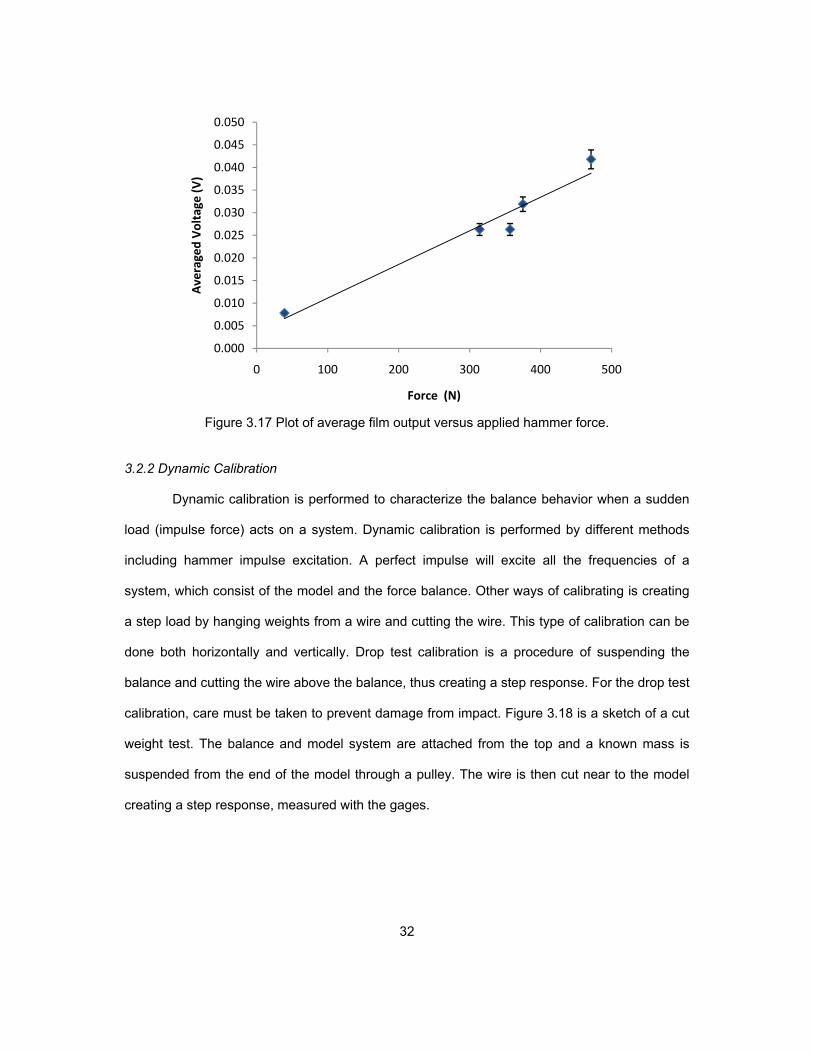
constant can be determined. The trendline equation of V=7E-05F +0.003, R2=0.953 of figure
3.17, shows the linear relation formed by averaging output of different hammer hits, with
different force values.
Mass (lbs) Force (N) Strain gage output voltage (V)
Loading of weight Unloading of weight
0 0.0 0.000 0.000
20 88.9 0.025 0.030
40 177.9 0.047 0.054
60 266.8 0.071 0.077
80 355.8 0.097 0.101
100 444.8 0.119 0.132
120 533.7 0.141 0.156
140 622.7 0.167 0.178
160 711.7 0.188 0.209
180 800.6 0.212 0.232
200 889.6 0.232 0.257
220 978.6 0.254 0.280
240 1067.5 0.276 0.304
260 1156.5 0.298 0.321
280 1245.5 0.320 0.339
300 1334.4 0.349 0.355
320 1423.4 0.369 0.373
32
0.000
0.005
0.010
0.015
0.020
0.025
0.030
0.035
0.040
0.045
0.050
0 100 200 300 400 500
Averaged Voltage (V)
Force (N)
Figure 3.17 Plot of average film output versus applied hammer force.
3.2.2 Dynamic Calibration
Dynamic calibration is performed to characterize the balance behavior when a sudden
load (impulse force) acts on a system. Dynamic calibration is performed by different methods
including hammer impulse excitation. A perfect impulse will excite all the frequencies of a
system, which consist of the model and the force balance. Other ways of calibrating is creating
a step load by hanging weights from a wire and cutting the wire. This type of calibration can be
done both horizontally and vertically. Drop test calibration is a procedure of suspending the
balance and cutting the wire above the balance, thus creating a step response. For the drop test
calibration, care must be taken to prevent damage from impact. Figure 3.18 is a sketch of a cut
weight test. The balance and model system are attached from the top and a known mass is
suspended from the end of the model through a pulley. The wire is then cut near to the model
creating a step response, measured with the gages.

33
Figure 3.18 Sketch of a cut weight test.
Cut weight test was also performed vertically, since vibrations can occur in the step response
when using a pulley as support. This arrangement is seen in figure 3.19.
Figure 3.19 Vertical cut weight test
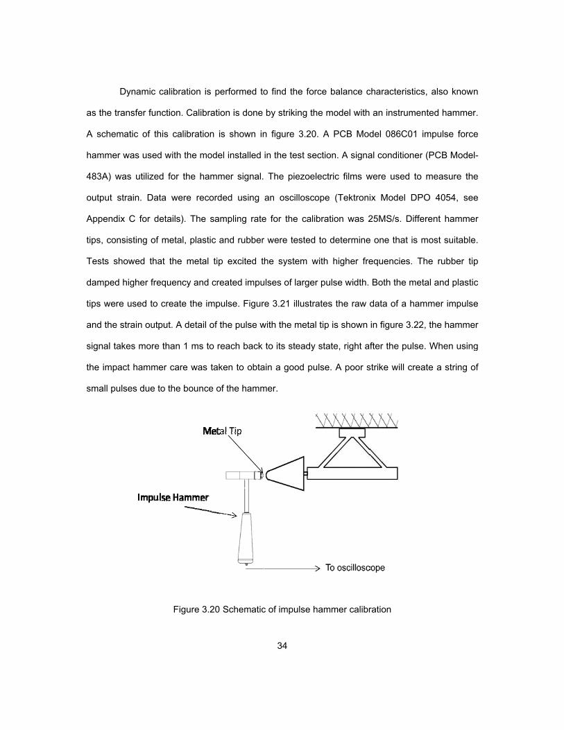
as th
A sc
hamm
483A
outpu
Appe
tips,
Tests
damp
tips w
and t
signa
the im
smal
Dynamic
he transfer fun
chematic of th
mer was used
A) was utilize
ut strain. Da
endix C for d
consisting of
s showed tha
ped higher fre
were used to
the strain out
al takes more
mpact hamm
l pulses due t
calibration is
nction. Calibra
his calibration
d with the mo
ed for the ham
ata were reco
details). The s
f metal, plasti
at the metal
equency and
create the im
put. A detail o
e than 1 ms to
er care was t
to the bounce
Figure 3.2
performed to
ation is done
n is shown in
odel installed
mmer signal.
orded using
sampling rate
c and rubber
tip excited t
created impu
mpulse. Figur
of the pulse w
o reach back
taken to obta
e of the hamm
20 Schematic
34
o find the for
by striking th
n figure 3.20
in the test se
The piezoel
an oscillosco
e for the calib
r were tested
he system w
ulses of larger
re 3.21 illustra
with the metal
to its steady
ain a good pu
mer.
c of impulse h
rce balance c
he model with
. A PCB Mo
ection. A signa
ectric films w
ope (Tektron
bration was 2
to determine
with higher fre
r pulse width.
ates the raw
tip is shown
state, right a
ulse. A poor s
hammer calibr
characteristics
h an instrumen
del 086C01
al conditioner
were used to
ix Model DP
25MS/s. Diffe
e one that is m
equencies. T
Both the met
data of a ham
in figure 3.22
after the pulse
strike will crea
ration
s, also known
nted hammer
impulse force
r (PCB Model
measure the
PO 4054, see
erent hamme
most suitable
The rubber tip
tal and plastic
mmer impulse
2, the hamme
e. When using
ate a string o
n
r.
e
-
e
e
er
e.
p
c
e
er
g
of

Figurtaken
F
re 3.21 Raw n over duratio
Figure 3.22 Sa
data of a haon of 150 ms
ample hamme
ammer impuls(below).
er impulse cre
35
se (above) an
eated by strik
nd the respon
king the metal
nse of the ha
l tip on the mo
ammer impac
odel cone.
ct

36
To form the transfer function (impulse response), the obtained strain output is
deconvolved with the hammer impulse. As mentioned before, a poor hammer strike can result in
obtaining an inaccurate transfer function. The hammer strike can be verified, since theoretically
convolution of an ideal impulse with a unit step results in a perfect step response. Matlab™ was
used to create a unit step (start at t=0) as shown in figure 3.25. The hammer impulse was
convolved with this unit step. The resultant convolved signal is illustrated in figure 3.23. This
signal was compared with a simulated step response, which is formed by convolving a modified
impulse with the unit step [9]. This modified impulse was created by padding zeroes right after
the pulse of the hammer strike, as shown in figure 3.26. The pulse was identified to have a
width of approximately 487µs, as illustrated in figure 3.27.
Figure 3.23 Check signal of both raw hammer signal and modified hammer signal.
A detailed view of the check signal is shown in figure 3.24. The error bar shows the
deviation of the signal from the modified pulse signal. The hammer check signal agrees with the
perfect step response. An error estimate on the signal shows variation of ± 0.6 %. It may be
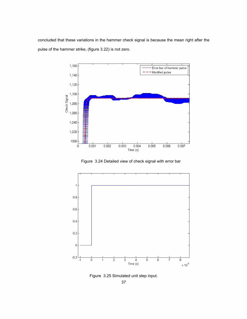
conc
pulse
cluded that the
e of the hamm
ese variations
mer strike, (fig
Figure
Fi
s in the hamm
gure 3.22) is n
e 3.24 Detaile
igure 3.25 Si
37
mer check sig
not zero.
ed view of che
imulated unit
gnal is becaus
eck signal wit
step input.
se the mean
th error bar
right after the
e
from
Figurappro
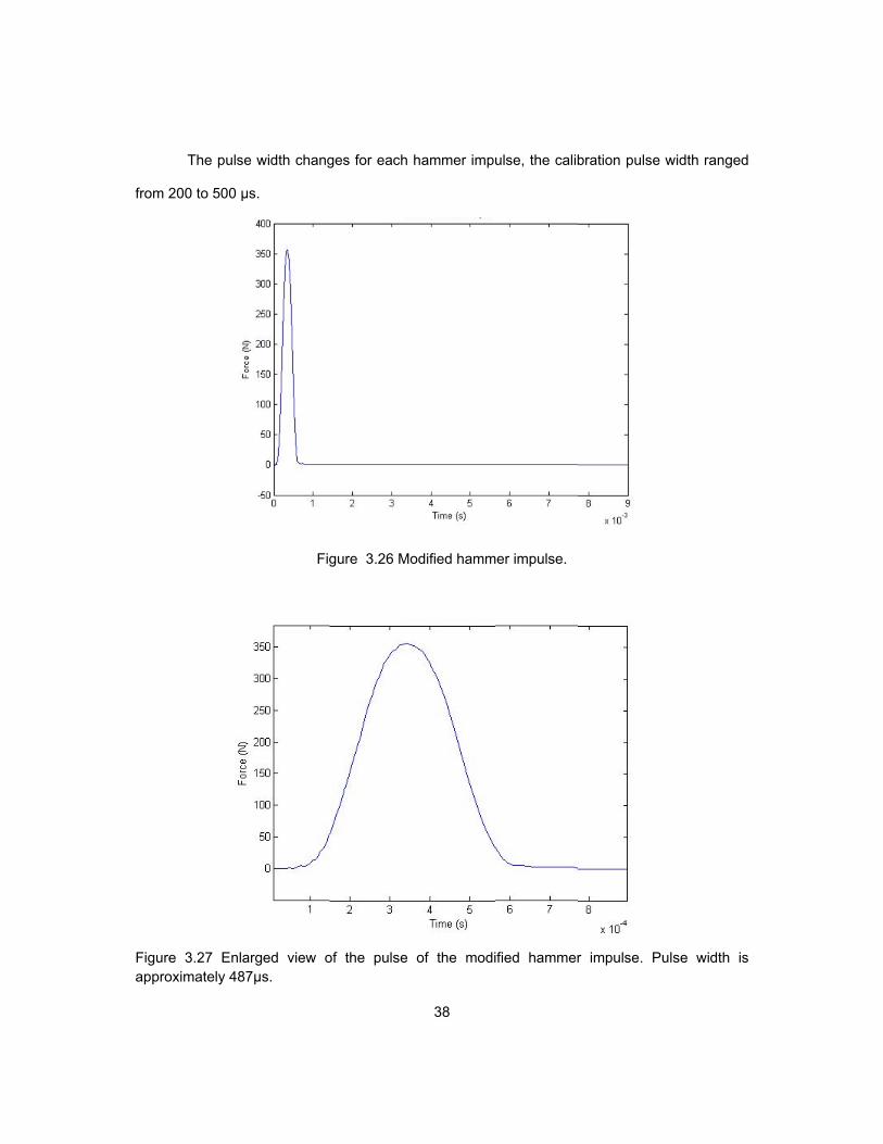
The pulse
200 to 500 µ
re 3.27 Enlaoximately 487
e width chang
s.
Fig
arged view o7µs.
ges for each
gure 3.26 Mo
of the pulse
38
hammer impu
odified hamm
of the modi
ulse, the calib
mer impulse.
ified hammer
bration pulse
r impulse. P
width ranged
ulse width is
d
s
was
was
using
figure
each
deco
frequ
FigurJMEC
funct
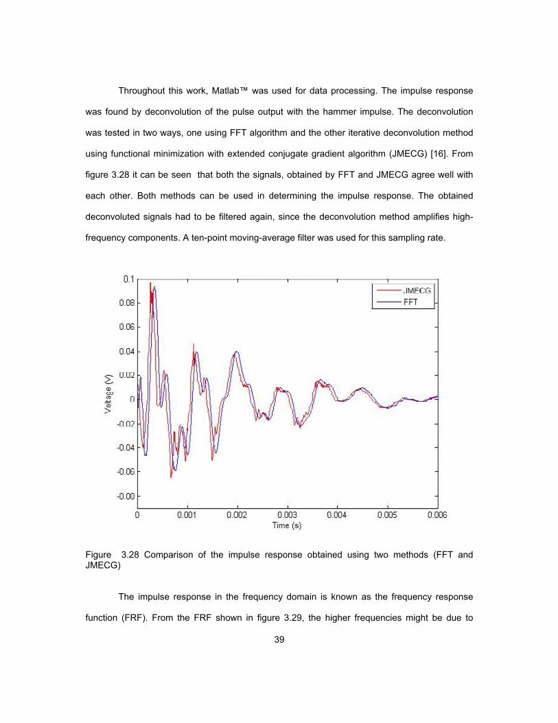
Througho
found by dec
tested in two
g functional m
e 3.28 it can
h other. Both
onvoluted sign
uency compon
re 3.28 ComCG)
The impu
tion (FRF). F
out this work,
convolution o
o ways, one u
minimization w
be seen tha
methods ca
nals had to b
nents. A ten-p
mparison of
ulse response
From the FRF
Matlab™ wa
of the pulse o
using FFT alg
with extended
at both the sig
an be used in
be filtered aga
point moving-
the impulse
e in the frequ
F shown in fi
39
as used for d
output with th
gorithm and th
d conjugate g
gnals, obtaine
n determining
ain, since the
-average filter
response ob
uency domain
igure 3.29, th
data processi
he hammer im
he other itera
gradient algo
ed by FFT an
g the impulse
e deconvoluti
r was used fo
btained using
n is known a
he higher fre
ng. The impu
mpulse. The d
ative deconvo
rithm (JMECG
nd JMECG ag
e response.
on method a
or this samplin
g two metho
as the freque
quencies mig
ulse response
deconvolution
lution method
G) [16]. From
gree well with
The obtained
amplifies high
ng rate.
ods (FFT and
ncy response
ght be due to
e
n
d
m
h
d
-
d
e
o

intern
syste
spec
Figurfrequ
nal reflection
em character
ctrum of the si
re 3.29 Poweuencies.
Figure 3
of stress w
istics. A deta
ignal is illustra
er spectral d
3.30 Enlarged
aves. The re
ailed view of t
ated figure 3.
ensity plot of
d power spec
40
esulting frequ
the first 12 k
31.
f frequency r
ctral density p
uency respon
kHz is shown
response fun
lot of FRF for
nse describes
in figure 3.3
ction showin
r the first 12 k
s the balance
0. The phase
g the various
kHz.
e
e
s
which
trans
frequ
red. T
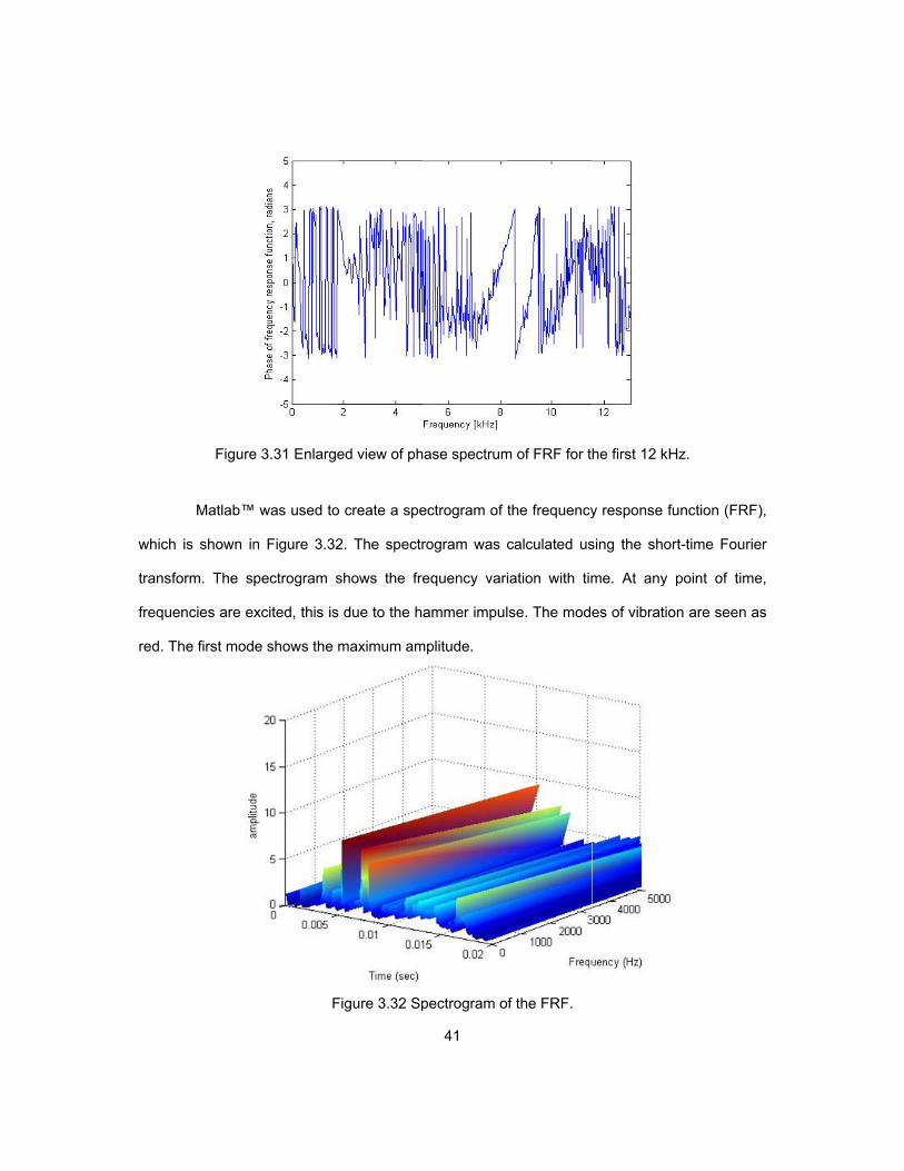
Figure
Matlab™
h is shown in
sform. The s
uencies are e
The first mod
e 3.31 Enlarge
was used to
n Figure 3.32
pectrogram s
xcited, this is
e shows the
F
ed view of ph
o create a spe
2. The spectr
shows the fre
s due to the h
maximum am
Figure 3.32 Sp
41
ase spectrum
ectrogram of t
rogram was c
equency vari
ammer impul
mplitude.
.
pectrogram o
m of FRF for t
the frequency
calculated us
iation with tim
lse. The mod
f the FRF.
he first 12 kH
y response fu
sing the shor
me. At any p
es of vibratio
Hz.
unction (FRF)
rt-time Fourie
point of time
n are seen as
),
er
e,
s
42
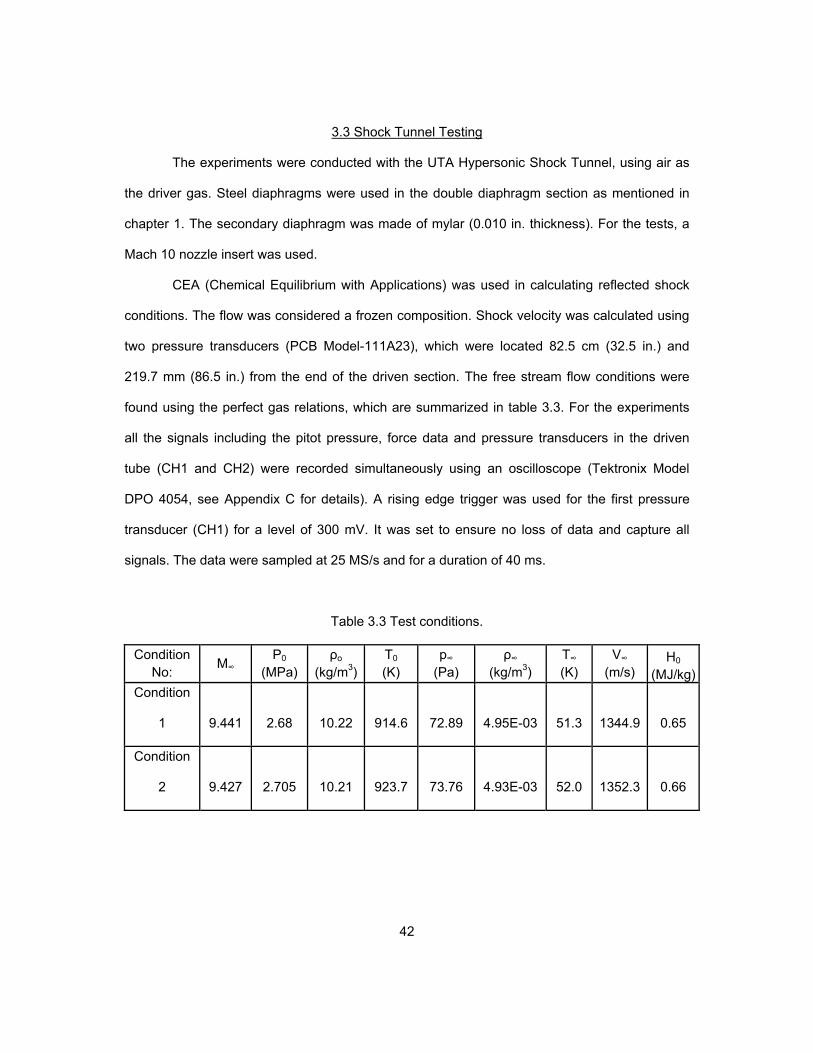
3.3 Shock Tunnel Testing
The experiments were conducted with the UTA Hypersonic Shock Tunnel, using air as
the driver gas. Steel diaphragms were used in the double diaphragm section as mentioned in
chapter 1. The secondary diaphragm was made of mylar (0.010 in. thickness). For the tests, a
Mach 10 nozzle insert was used.
CEA (Chemical Equilibrium with Applications) was used in calculating reflected shock
conditions. The flow was considered a frozen composition. Shock velocity was calculated using
two pressure transducers (PCB Model-111A23), which were located 82.5 cm (32.5 in.) and
219.7 mm (86.5 in.) from the end of the driven section. The free stream flow conditions were
found using the perfect gas relations, which are summarized in table 3.3. For the experiments
all the signals including the pitot pressure, force data and pressure transducers in the driven
tube (CH1 and CH2) were recorded simultaneously using an oscilloscope (Tektronix Model
DPO 4054, see Appendix C for details). A rising edge trigger was used for the first pressure
transducer (CH1) for a level of 300 mV. It was set to ensure no loss of data and capture all
signals. The data were sampled at 25 MS/s and for a duration of 40 ms.
Table 3.3 Test conditions.
Condition No:
M∞ P0
(MPa) ρo
(kg/m3) T0 (K)
p∞ (Pa)
ρ∞ (kg/m3)
T∞ (K)
V∞ (m/s)
H0 (MJ/kg)
Condition
1 9.441 2.68 10.22 914.6 72.89 4.95E-03 51.3 1344.9 0.65
Condition
2 9.427 2.705 10.21 923.7 73.76 4.93E-03 52.0 1352.3 0.66
43
CHAPTER 4
RESULTS AND DISCUSSIONS
4.1 Force Measurement Prediction
4.1.1 Modified Newtonian Theory
Newtonian theory assumes that the oncoming flow can be considered of as continuous
stream of particles. When the particles hit a surface at high speeds, they lose all their
momentum perpendicular to the surface. The pressure coefficient predicted by Newtonian
theory is given by
2sin (4.1)
This equation shows that the pressure distribution is related to the square of the inclination
angle. The modified Newtonian theory was proposed by Lees in 1955 so that the pressure is a
function of M∞:
, 1 (4.2)
where, Cp,max is the maximum pressure coefficient behind a normal shock wave, at the
stagnation point. ∞
is calculated using the Rayleigh pitot formula [18] :
(4.3)
44
The axial force coefficient is calculated by the following relation [17],
2C , 0.25 cos 1 sin (4.4)
0.125 sin cos
cos sin 0.50 sin cos
⁄ cos
tan cos
⁄ cos
2tan
where,
RN is the nose radius of the blunt cone
RB is the base radius of the blunt cone
θc is the half cone angle
α is the angle of attack
The normal force coefficient is calculated by the following relation [17],
2C , 0.25 cos (4.5)
cos
⁄
⁄
2
The following relation is used to calculate Lift-to-Drag ratio:
(4.6)
Drag
Eqns
The
of an
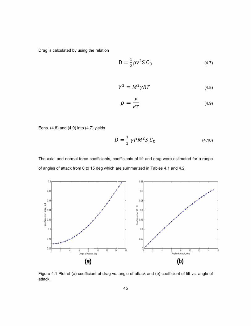
Figurattac
g is calculated
s. (4.8) and (4
axial and nor
ngles of attack
re 4.1 Plot of ck.
d by using the
4.9) into (4.7)
rmal force co
k from 0 to 15
(a) coefficien
e relation
yields
efficients, coe
5 deg which a
nt of drag vs.
45
D ρv
efficients of li
are summarize
angle of atta
S C
ift and drag w
ed in Tables 4
ack and (b) co
were estimate
4.1 and 4.2.
oefficient of li
(4.7
(4.8
(4.9
(4.10
ed for a range
ft vs. angle o
)
8)
9)
)
e
of
46
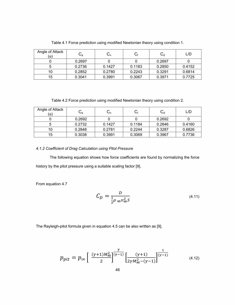
Table 4.1 Force prediction using modified Newtonian theory using condition 1.
Angle of Attack
(α) Ca Cn Cl Cd L/D
0 0.2697 0 0 0.2697 0 5 0.2736 0.1427 0.1183 0.2850 0.4152 10 0.2852 0.2780 0.2243 0.3291 0.6814 15 0.3041 0.3991 0.3067 0.3971 0.7725
Table 4.2 Force prediction using modified Newtonian theory using condition 2.
Angle of Attack (α) Ca Cn Cl Cd L/D
0 0.2692 0 0 0.2692 0 5 0.2732 0.1427 0.1184 0.2846 0.4160 10 0.2848 0.2781 0.2244 0.3287 0.6826 15 0.3038 0.3991 0.3069 0.3967 0.7736
4.1.2 Coefficient of Drag Calculation using Pitot Pressure
The following equation shows how force coefficients are found by normalizing the force
history by the pitot pressure using a suitable scaling factor [9],
From equation 4.7
(4.11)
The Rayleigh-pitot formula given in equation 4.5 can be also written as [9],
(4.12)

47
For high values of M∞, when 2 ≫ 1 , equation 4.12 can be approximated as,
(4.13)
(4.14)
(4.15)
Substituting these into equation 4.13 we get
(4.16)
Substituting in equation 4.16
(4.17)
For a given flow condition and S remain constant, therefore drag coefficient is expressed as
(4.18)
Measuring the pitot pressure along with the force during an experiment can be used to estimate
the force coefficient, which also varies with time.
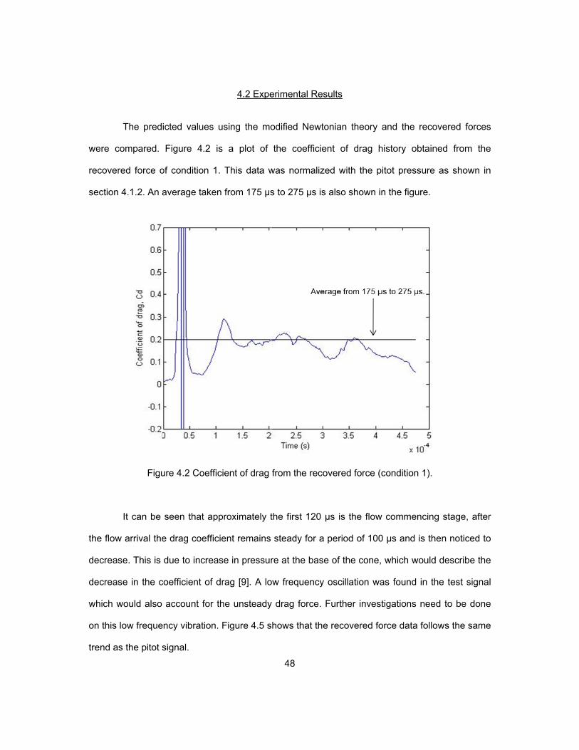
were
recov
secti
the fl
decre
decre
which
on th
trend
The pred
e compared.
vered force o
on 4.1.2. An a
Figu
It can be
low arrival the
ease. This is
ease in the c
h would also
his low freque
d as the pitot s
icted values
Figure 4.2
of condition 1
average take
ure 4.2 Coeffi
seen that ap
e drag coeffic
due to increa
coefficient of d
account for
ency vibration
signal.
4.2 Expe
using the mo
is a plot of
. This data w
n from 175 µs
cient of drag
pproximately t
cient remains
ase in pressu
drag [9]. A lo
the unsteady
. Figure 4.5 s
48
erimental Res
odified Newto
the coefficie
was normaliz
s to 275 µs is
from the reco
the first 120
steady for a
re at the base
ow frequency
y drag force.
shows that the
sults
onian theory
ent of drag h
ed with the p
s also shown
overed force (
µs is the flow
period of 100
e of the cone
oscillation w
Further inves
e recovered fo
and the reco
history obtain
pitot pressure
in the figure.
(condition 1).
w commencin
0 µs and is th
, which would
was found in t
stigations nee
orce data follo
overed forces
ned from the
e as shown in
ng stage, afte
hen noticed to
d describe the
the test signa
ed to be done
ows the same
s
e
n
r
o
e
al
e
e
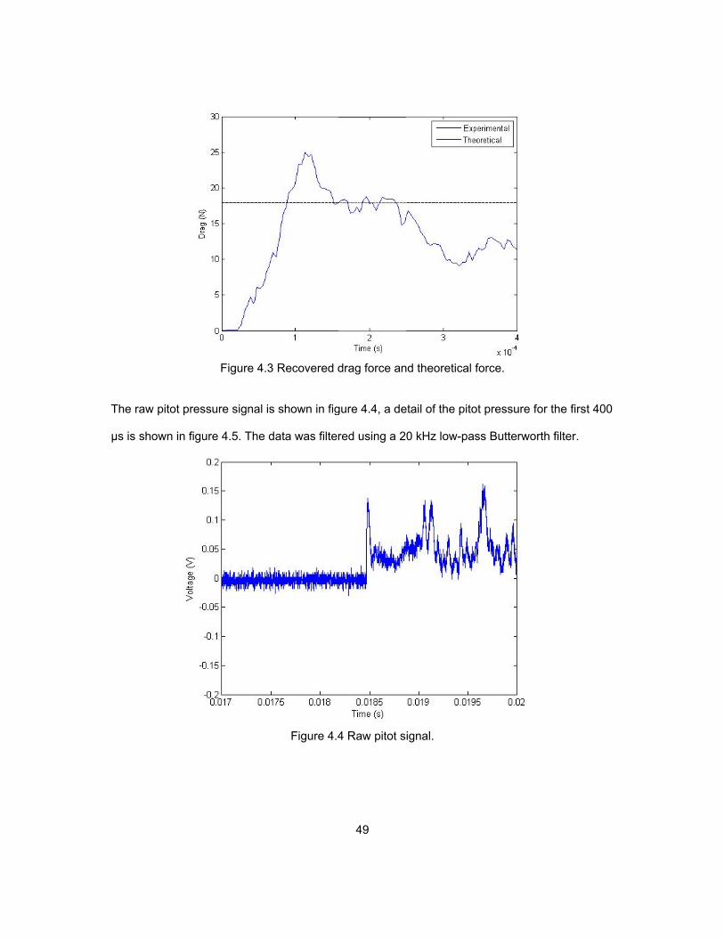
The r
µs is
raw pitot pres
shown in figu
Figure 4.3
ssure signal is
ure 4.5. The d
3 Recovered d
s shown in fig
data was filter
Figure 4.4
49
drag force an
gure 4.4, a de
red using a 2
4 Raw pitot s
nd theoretical
etail of the pito
0 kHz low-pa
ignal.
force.
ot pressure fo
ss Butterwort
or the first 400
th filter.
0
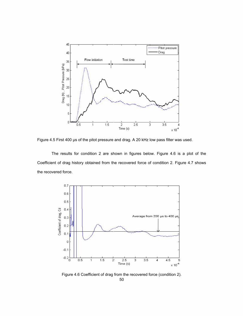
Figur
Coef
the re
re 4.5 First 40
The resu
fficient of dra
ecovered forc
Figu
00 µs of the p
lts for condit
g history obta
ce.
ure 4.6 Coeffi
pitot pressure
tion 2 are sh
ained from th
cient of drag 50
and drag. A 2
hown in figur
he recovered
from the reco
20 kHz low pa
res below. F
force of con
overed force (
ass filter was
igure 4.6 is
dition 2. Figu
(condition 2).
used.
a plot of the
ure 4.7 shows
e
s
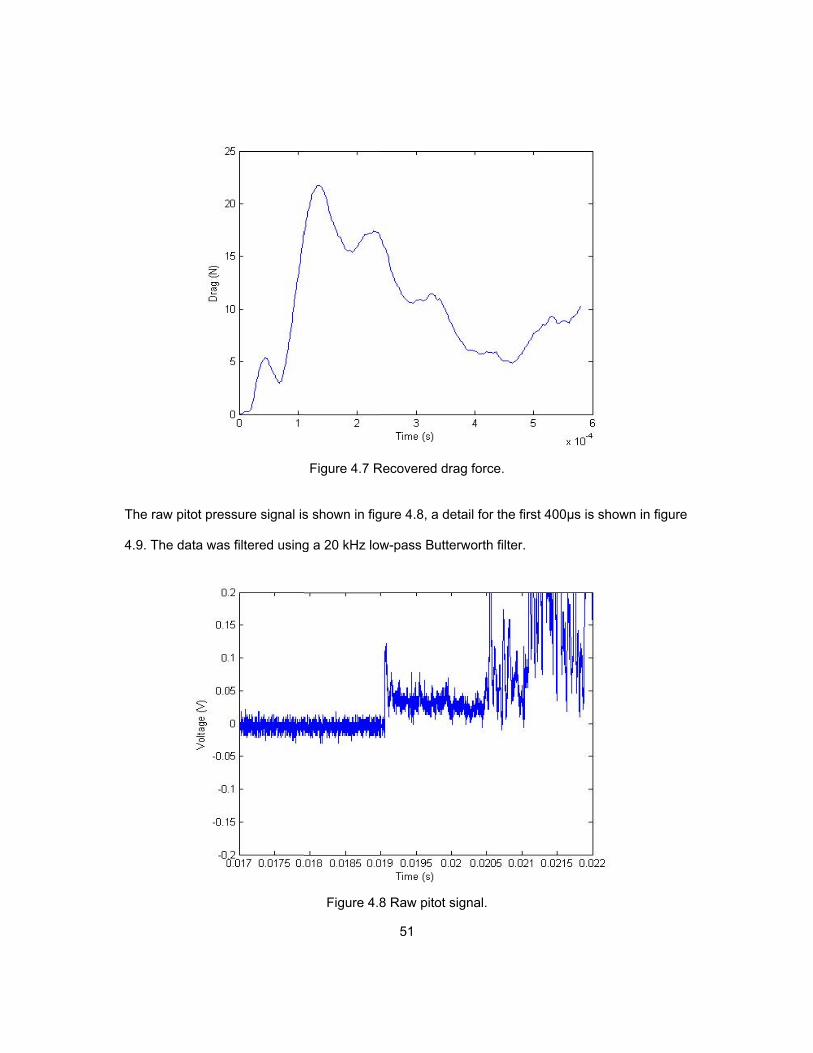
The r
4.9. T
raw pitot pres
The data was
ssure signal is
s filtered using
Figure 4.7 R
s shown in fig
g a 20 kHz low
Figure 4.8
51
Recovered dra
gure 4.8, a de
w-pass Butte
8 Raw pitot s
ag force.
etail for the firs
rworth filter.
ignal.
st 400µs is shhown in figuree

From
meas
table
varia
detai
C
Figure 4.9
m the experim
sured pitot p
e 4.3. Δ % i
ations seen in
il in chapter 5
Condition no
1
2
9 First 400 µs
mental results
ressure. The
is the differe
n the recovere
5.
Table 4.3 C
: Drage(N)
16.9 ± 8
13.6 ± 1
s of the pitot p
s it is seen
e experimenta
ence betwee
ed drag, migh
Comparison o
exp Dra
8.9 % 1
9.6 % 1
52
pressure. A 2
that the reco
al to theoretic
en the theor
ht be due to
of experimenta
agtheory (N)
17.9
18.0
0 kHz low-pa
overed drag
cal drag com
retical and e
several facto
al to theoretic
Δ %
5.9
32.3
ass filter was u
is in accorda
mparison is su
experimental
ors, which are
cal drag
Coefficientcoeffic
0.199 ±
0.128 ±
used.
ance with the
ummarized in
values. The
e discussed in
t of drag ient
± 7.8
± 27.9
e
n
e
n
53
CHAPTER 5
CONCLUSION AND FUTURE WORK
Due to the short duration in impulse hypersonic shock tunnels, it is difficult to measure
accurately the aerodynamic forces. Since the test time is very small, force equilibrium may not
be reached between the model and the balance structure. The stress wave force balance
(SWFB) is a method used to analyze the stress waves formed during aerodynamic loading.
5.1 Force Balance in the UTA Hypersonic Shock Tunnel
A force balance was designed for measuring forces on aerodynamic models. In the
present work, drag was measured for a blunt cone using the force balance. The force balance
system included the model, which was fabricated in steel and the force balance, made of 6061
aluminum alloy. Several designs were investigated before the actual fabrication. Some of the
limitations in the design included the size of the balance, amount of load the balance must
withstand, model and support attachment and machining simplicity. The force balance was
designed to fit in the hypersonic shock tunnel test section, allowing room for support
attachments, model attachment and wiring. FEA (Finite Element Analysis) was used to
determine the dynamic characteristics of the force balance under high impact loading. It was
also performed to be certain of the maximum loads the force balance could resist.
Piezoelectric film gages and strain gages were used to measure forces. Both static and
dynamic calibrations were performed. The static calibration involved loading the force balance
with increments of known weights and measuring the strain for each weight. The same
procedure was also done for unloading the weights. These results were plotted to obtain a
linear relationship. Dynamic calibration was done by pulse excitation using an impulse force
hammer. The input by a hammer hit and the output was obtained from the piezoelectric film
54
gages. From the impulse hammer tests an impulse response/ transfer function was determined.
Another dynamic calibration carried out was vertical and horizontal cut weight tests. These tests
involved hanging known weights to the model by steel wires and cutting the wire, thereby
creating a step load. These step loads were deconvoluted with the obtained transfer function to
recover the step input.
The model used in experiments was a blunt cone made of steel. It was designed such
that a pitot pressure measurement was taken simultaneously. The model and balance assembly
was then installed from the top in the test section. The required wiring was taken out of the test
section through drilled bolts, which were sealed. The instrumented gages were shielded to
prevent electromagnetic interference and sealed in rubber and electrical tape. Tests were
conducted with conditions mentioned in chapter 4. All the data signals including the pitot
pressure, force data and pressure transducers in the driven tube (CH1 and CH2) were recorded
simultaneously using an oscilloscope ( see Appendix C).
The strain data was processed and deconvolved with the transfer function, to recover
the drag. Deconvolution was performed using an iterative algorithm [16]. A low frequency
vibration was noticed in the signal of the measured force, before the incident shock reached the
pressure transducers in the driven tubes. From each of the primary tests, this mentioned
vibration occurred, which led to the conclusion that a vibration is due to the test section
movement. An approach was made to tighten down the test section using steel wire rope and
turnbuckles. Tests showed that these oscillations persisted. Therefore, it may be concluded that
stress waves formed by the sudden rupture of the diaphragms have affected the drag
measurements.
55
5.2 Future Work and Recommendations
The following points may be included for future work for force measurements:
Develop an isolation system to reduce the initial vibrations in the force signal.
Force measurement with other models
Analyzing the flow with CFD simulations.
Tests at different enthalpy levels.
Calculate three components of force, such as, lift, drag and pitching moment.
Compensation of inertial forces due to tunnel movement using accelerometers.
Analyze signals in time-frequency representation using wavelet transform.
From the recovered drag, it can be seen that the signal follows the pitot pressure but
that there is also a fluctuation in drag, which is accounted by the occurrence of these low
frequency vibration. Further investigations need to be done on developing methods to decrease
these low frequency oscillations, by using springs, rubber dampers etc. Some of the
recommendation include, but are not limited to tests with simple shield design and compare the
results. Also, test the model at different angle of attacks and compare the drag. Care must also
be taken with the piezoelectric films, since they are very sensitive to EMI (electromagnetic
interference). Any power source close to the tunnel must be avoided, which can result in
erroneous values.

56
APPENDIX A
LIST OF DESIGN DRAWINGS

57
Figure A.1 Force balance drawing.

58
Figure A.2 Blunt cone model drawing.
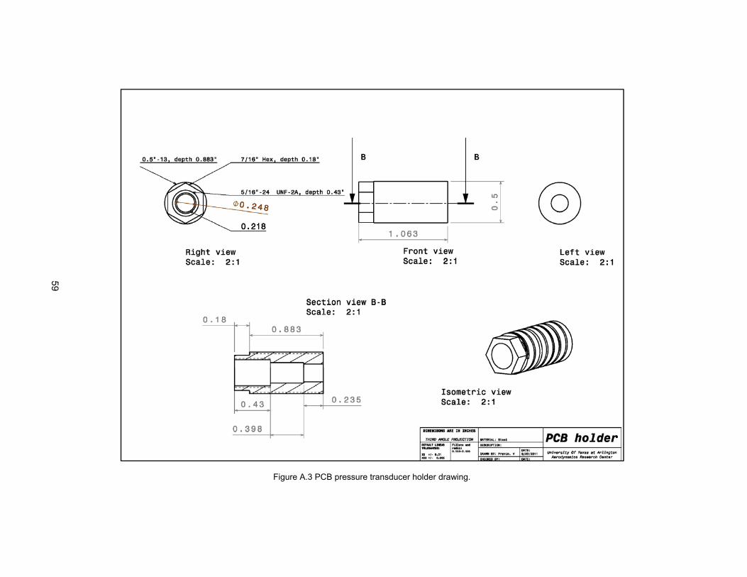
59
Figure A.3 PCB pressure transducer holder drawing.

60
Figure A.4 Hinge joint part 1 drawing.

61
Figure A.5
5 Hinge part 2 drawwing.
62
Figure A.6 Scoring pattern on steel diaphragm drawing (courtesy Tiago Rolim).

63
APPENDIX B
MATLAB PROGRAM FOR FORCE ESTIMATION

64
%xxx Program to calculate Axial, Normal force coefficient and L/D xxx% xxxxxxxxxxxxxxxxxxxxxxxxxxxxxxxxxxxxxxxxxxxxxxxxxxxxxxxxxxxxxxxxxxxxx clc clear all for j=1:4 in=input('*********************\nTo find Axial,Normal force coefficient and L/D press 1: \nTo find Cpt press 2:\nTo find Pressure ratio press 3:\n********************* '); Rb=1.65; Rn=0.355; theta=9; phi=asin(cos(theta)); r=0; L=0; d=Rb/Rn; gamma=1.4; M=4.3; if in==3 %%%xxxxxxxxxxxxxxxxxxx pressure ratio calculation xxxxxxxxxxxxx Cpt=input('Enter Cpt , if known : ') ; gamma=input('Enter specific heat ratio : '); M=input('Enter Mach no: '); pressure_ratio =(((gamma+1)*M^2)/2)^(gamma/(gamma- 1))*((gamma+1)/((2*gamma*M^2)-(gamma-1)))^(1/(gamma-1)) x=pressure_ratio; plot(M,x ,'*b'); xlabel('Mach no: ,M') ylabel('Pressure ratio , Pt2/P1') %xxxxxxxxxxxxxxxxxxxxxxxxxxxxxx Cpt calculation xxxxxxxx elseif in~=(1:3) return elseif in==2 x=input('Enter pressure ratio : '); gamma=input('Enter specific heat ratio : '); M=input('Enter Mach no: '); Cpt=(((x)-1)*(2/(gamma*M^2))) %%%xxxxxxxxxxxxxxxxxxxxxxx L/D xxxxxxxxxxxxxxxxxxx elseif in==1
65
for i=1:1 Cpt= input('Enter Cpt: '); Rb=input('Enter Base Radius: '); Rn=input('Enter Nose Radius: '); theta=input('Cone half Angle : '); phi=asin(cos(theta)); r=0; x=0; L=0; d=Rb/Rn; gamma=input('Enter specific heat ratio : '); M=input('Enter Mach no: '); alpha=-15:0.5:15; Cp=Cpt*(sind(theta))^2 plot(alpha,Cp,'*r') hold on xlabel('Angle of Attack,Alpha') ylabel('Axial Force Coefficient, Ca') a=2*Cpt*((Rn^2)/Rb^2); b=0.25.*(cosd(alpha).^2).*(1-(sind(theta)^4))+(0.125.*(sind(alpha).^2)*(cosd(theta).^4)); c=((tand(theta).*((cosd(alpha).^2)*(sind(theta).^2)+0.5.*(sind(alpha).^2).*(cosd(theta).^2))).*((((d-cosd(theta)).*cosd(theta))/tand(theta))+(((d-cosd(theta)).^2)/(2*tand(theta))))); Ca=a*(b+c); plot(alpha,Ca,'*-r') hold on title('Axial Force Coefficient vs Angle of Attack (Alpha)') xlabel('Angle of Attack, Alpha') ylabel('Axial Force Coefficient, Ca') p=2*Cpt*((Rn^2)/Rb^2); q=0.25.*sind(alpha).*cosd(alpha).*(cosd(theta)^4); r=(sind(alpha).*cosd(alpha).*sind(theta).*cosd(alpha).*((((d-cosd(theta)).*cosd(theta))/tand(theta))+(((d-cosd(theta)).^2)/(2*tand(theta))))); Cn=p*(q+r); figure plot(alpha,Cn,'*-black') title('Normal Force Coefficient vs Angle of Attack (Alpha)') xlabel('Angle of Attack,Alpha') ylabel('Normal Force Coefficient, Cn') CL=((Cn.* cosd(alpha))-(Ca.*sind(alpha))); CD=((Cn.* sind(alpha))+(Ca.*cosd(alpha))); L_D= CL./CD figure
66
plot(alpha,L_D,'*-g') drawnow title('L/D ratio vs Angle of Attack (Alpha)') xlabel('Angle of Attack,Alpha') ylabel('L/D ') hold on end end end

67
APPENDIX C
INSTRUMENTATION DETAILS

68
C.1 Data acquisition
Manufacturer: Tektronix Digital Phosphor Oscilloscope. Model: DPO 4054
Features: Analog bandwidth – 500 Mhz Sample rate – 2.5 GS/s Record length – 20 M points Analog channels – 4
C. 2 Strain measurements
Manufacturer: Measurement specialties Model: DT1-052k Features: Min. impedance – 1MΩ
Output voltage – mV to 100’s of volt Operating temp – -40 to 60°C
Manufacturer: Omega engineering, Inc. Model: SGD-3/120-LY13 Features: Max Vrms – 4.5
Nom. Resistance – 120 Gage Factor – 2.0 ± 5% Operating temp – -75 to 200°C
C.4 Pressure Transducers
Manufacturer: PCB Piezotronics, Inc. Model: 111A23 Features: Measurement range – 10kpsi Sensitivity – 0.5mV/psi Maximum pressure – 15kpsi Operating temp – -73 to 135°C
69
Manufacturer: PCB Piezotronics, Inc. Model: 113A21 Features: Measurement range – 200psi Sensitivity – 25mV/psi Maximum pressure – 1000psi Operating temp – -73 to 135°C
C.7 Strain gage amplifier
Manufacturer: Paine instruments, Inc. Model: Strain gage amplifier Features: Excitation voltage range – 0-10V
Gain – 100
Amplifier circuit diagram used for piezoelectric films
Figure C.1 Circuit diagram of piezoelectric film amplifier. Circuit uses a LM-386 IC.
70
REFERENCES
[1] Robinson, M., “Simultaneous Lift, Moment and Thrust Measurements on a Scramjet in
Hypervelocity Flow,” Ph.D. dissertation, University of Queensland, 2003.
[2] Sanderson, S.R. and Simmons, J.M., “Drag Balance for Hypervelocity Impulse Facilities,” AIAA Journal, Vol. 29, No. 12, pp. 2185–2191, 1991.
[3] Daniel, W.J.T. & Mee, D.J., “Finite Element Modelling of a Three-Component Force Balance
for Hypersonic Flows,” Computers and Structures 54 (1), 3548, 1995. [4] Robinson, M., Schramm, J.M. and Hannemann, K., “An Investigation into Internal and
External Force Balance Configurations for Short Duration Wind Tunnels,” Notes on
Numerical Fluid Mechanics and Multidisciplinary Design, Volume 96/2008,129-136, 2008. [5] Boyce, R. R. and Stumvoll, A., ”Re-entry Body Drag: Shock Tunnel Experiments and
Computational Fluid Dynamics Calculations Compared,” Shock Waves, 16 6: 431-443, 2007.
[6] Kulkarni, V. and Reddy, K.P.J., ”Accelerometer-Based Force Balance for High Enthalpy
Facilities,” J. Aerosp. Engrg. 23, 276 doi:10.1061/(ASCE), 2010. [7] Sahoo,N, Mahapatra, D.R., Jagadeesh, G., Gopalakrishnan, S. and Reddy, K.P.J., ”Design
and Analysis of a Flat Accelerometer-based Force Balance System for Shock Tunnel Testing,” Measurement, 40 (1).pp.93-106, 2007.
[8] Sahoo, N., Suryavamshi, K., Reddy, K.P.J. and Mee, D.J., ”Dynamic Force Balances for
Short-Duration Hypersonic Testing Facilities,” Experiments in Fluids, 38 (5). pp. 606-614, 2005.
[9] Mee, D.J., “Dynamic Calibration of Force Balances,” Centre for Hypersonics, The University
of Queensland, Australia. Tech. Rep. 2002/6, Jan 2003.
71
[10] Smith, A. L.; Mee, D.J., “Drag Measurements in a Hypervelocity Expansion Tube,” Shock
Waves, Volume 6, Issue 3, pp. 161-166,1996.
[11] Marineau, E., “Force Measurements in Hypervelocity Flows with an Acceleration
Compensated Piezoelectric Balance,” Journal of Spacecraft and Rockets, 0022-4650
vol.48, no.4 (697-700), 2011.
[12] Smith, S.W., The Scientist and Engineer's Guide to Digital Signal Processing.
[Online],http://www.dspguide.com/, 2012.
[13] Murtugudde, R.G., "Hypersonic Shock Tunnel," Master's Thesis, Department of Aerospace Engineering, The University of Texas at Arlington, Arlington, TX, 1986. [14] Stuessy, W.S, "Hypersonic Shock Tunnel Development and Calibration," Master's Thesis, Department of Aerospace Engineering, The University of Texas at Arlington, Arlington, TX, 1989. [15] Stuessy, W.S., Murtugudde, R.G., Lu, F.K. and Wilson, D.R., "Development of the UTA
Hypersonic Shock Tunnel," Paper 90-0080, AIAA 28th Aerospace Sciences Meeting, January 8-11, Reno, Nevada, 1990.
[16] Prost, R., Goutte, R., “Discrete Constrained Iterative Deconvolution Algorithms with
Optimized Rate of Convergence,” Signal Process.7(3), 209–230,1984.
[17] Bertin, J.J. Hypersonic Aerothermodynamics. American Institute of Aeronautics and
Astronautics, Inc., Washington, DC, 1994.
[18] Anderson, J.D. Fundamentals of Aerodynamics. New York, NY: McGraw-Hill, 2001.

72
BIOGRAPHICAL INFORMATION
Pravin Vadassery graduated with a Bachelors degree in Aeronautical engineering, his
endeavor to learn new things, lead him to the Masters degree in Aerospace engineering. His
passion for experiments and hands-on jobs helped him during his research at the Aerodynamic
Research Center. He has worked on many projects during his undergraduate and graduate
years, which included areas of design, analysis, and comparative studies. He plans to start his
career with all experience he gained and eventually establish his own company.