sensors

Article

Design and Optimization of FBG ImplantableFlexible Morphological Sensor to Realize theIntellisense for Displacement

Changbin Tian 1 ID , Zhengfang Wang 1,*, Qingmei Sui 1, Jing Wang 1,*, Yanan Dong 1, Yijia Li 1,Mingjuan Han 1, Lei Jia 1 and Hanpeng Wang 2

1 School of Control Science and Engineering, Shandong University, Jinan 250061, Chinachangbin_tian@163.com (C.T.); qmsui@sdu.edu.cn (Q.S.); dongyanan0115@163.com (Y.D.);liyijiasdu@163.com (Y.L.); han1772824165@126.com (M.H.); jialei@sdu.edu.cn (L.J.)

2 Geo & Stru Engineering Research Center, Shandong University, Jinan 250061, China; whp@sdu.edu.cn* Correspondence: Zfwang@sdu.edu.cn (Z.W.); wangjingkz@sdu.edu.cn (J.W.); Tel.: +86-151-6505-5501 (Z.W.);

+86-135-8904-4426 (J.W.)

Received: 13 June 2018; Accepted: 5 July 2018; Published: 19 July 2018�����������������

Abstract: The measurement accuracy of the intelligent flexible morphological sensor based onfiber Bragg grating (FBG) structure was limited in the application of geotechnical engineering andother fields. In order to improve the precision of intellisense for displacement, an FBG implantableflexible morphological sensor was designed in this study, and the classification morphologicalcorrection method based on conjugate gradient method and extreme learning machine (ELM)algorithm was proposed. This study utilized finite element simulations and experiments, in order toanalyze the feasibility of the proposed method. Then, following the corrections, the results indicatedthat the maximum relative error percentages of the displacements at measuring points in differentbending shapes were determined to be 6.39% (Type 1), 7.04% (Type 2), and 7.02% (Type 3), respectively.Therefore, it was confirmed that the proposed correction method was feasible, and could effectivelyimprove the abilities of sensors for displacement intellisense. In this paper, the designed intelligentsensor was characterized by temperature self-compensation, bending shape self-classification, anddisplacement error self-correction, which could be used for real-time monitoring of deformation fieldin rock, subgrade, bridge, and other geotechnical engineering, presenting the vital significance andapplication promotion value.

Keywords: FBG flexible sensor; morphological sensing; classification morphological correctionmethod; conjugate gradient method; ELM

1. Introduction

Fiber Bragg grating (FBG) is a promising sensing element for the fabrication of flexible sensorsowing to its advantageous characteristics, such as small size, light weight, water- and moisture-proofingabilities, and multiplex networking capacities. By embedding FBG into flexible substrates withproperties of high flexibility, high ductility, and free bending, flexible sensors were developedand extensively utilized in civil engineering, medical engineering, aerospace, and robotics etc.for the measurement of morphology, displacement, strain, and other measurands [1–4]. Recently,morphological sensing with FBG embedded flexible sensors has become a hot topic [5–8]. Payo et al. [9]measured the deflections of a robotic arm based on FBG sensors and interpolation methods.Xu et al. and Bhamber et al. [10,11] adopted orthogonal FBG arrays to measure bidirectionalcurvatures, then reconstructed shapes using a curve fitting algorithm. Yi et al. [12] studied a shape

Sensors 2018, 18, 2342; doi:10.3390/s18072342 www.mdpi.com/journal/sensors

Sensors 2018, 18, 2342 2 of 20

reconstruction method based on spatial movable coordinates, and realized the shape reconstructionof an aircraft frames. Kang et al. [13] modeled the relationship of wavelength–strain–displacementand reconstructed the entire structural deformations and local displacements of aluminum and acrylicbeam specimens. Also, Todd et al. [14] employed a material-adapted reference frame together with alocal linearization approach, for the purpose of reconstructing the shapes of slender. In the field ofgeotechnical engineering, researchers have studied the morphological sensing methods for measuringdisplacement profiles in critical areas of side slopes, subgrades, bridges, and other objects basedon the FBG embedded flexible sensors. Li et al. [15] established a deflection–strain relationship forFBG flexible rods, which was then used in physical model tests to measure the displacements of theunderground caves. Guo et al. [16] calculated the displacement profiles of beams using the strainsand rotation angles measured by the FBG sensing points. Kim N.S. et al. [17] measured the deflectioncurves using a regression analysis method, and then applied the method for the measurement ofbridge displacements. Xu et al. [18] estimated the bending deformations of the beams based on thecurvature functions of cross-sections.

In practical applications, several factors may affect the measurement accuracy of morphology,including the layout intervals of FBG, the strain transferring rate from the substrate to FBG, thecumulative errors induced by algorithm etc. Therefore, it is critical to correct the reconstructedshapes using effective methods, and to improve the shape measurement accuracy. In termsof morphological sensing error analyses and corrections, Zhang et al. [19] proposed a dynamicerror analysis method based on a least mean square algorithm. This method has been used forthe morphological reconstructions and error analyses of space plate structures. Sun et al. [20]experimentally calibrated the relationship between the wavelength and bending curvatures, andimproved the reconstruction precision of polyimide film deformations through the linear interpolationof the curvatures. Wang et al. [21,22] proposed an in situ calibrated deformation reconstruction methodfor FBG embedded geogrid, and improved the accuracy effectively. In the aforementioned research,unified correction coefficients were mainly applied to calibrate and correct the entire morphology of thestructure to be measured, as well as to improve the precision of the morphological sensing. However,it has been found that, in practice, due to the diversity of the measured structural morphologies, theunified coefficients have been difficult to be applicable to a variety of morphologies, leading to majordifferences of the correction results for different shapes. While the shape correction methods basedon the different morphological classifications for the FBG embedded flexible sensors have not yetbeen reported.

In this paper, a morphological sensing method, which is capable of correcting the reconstructedshape based on the morphological classification, was proposed to further improve the measurementaccuracy of FBG implantable flexible morphological sensors. First, an FBG implantable flexiblemorphological sensor with temperature self-compensation capabilities was developed, and an arccurve fitting based on morphological sensing algorithm was introduced. Then, temperature calibrationexperiment indicated that the temperature self-compensation could be realized by the differences inthe central wavelength variations of the two sensing points in the detecting unit. In the morphologicalcalibration experiment, a conjugate gradient method was adopted to define the correction coefficientsk of each morphology. A morphological sensing method which is capable of correcting the measuredshapes based on different morphological classifications was proposed. The classification of differentbending shapes was performed by using the extreme learning machine (ELM) algorithm. Finally,numerical simulations and experimental analyses were performed to verify the feasibility andeffectiveness of the proposed method. The results indicate that the proposed method can improve themorphological measurement accuracy of FBG implantable flexible morphological sensors effectively,and it is of vital significance for the measurement of displacement fields in subgrades, bridges, andother geotechnical engineering applications.

Sensors 2018, 18, 2342 3 of 20

2. Fabrication and Principle

2.1. Fabrication of the FBG Implantable Flexible Morphological Sensor

As detailed in Figure 1, for the proposed FBG implantable flexible morphological sensor,an acrylonitrile butadiene styrene (ABS) rod with high strength, corrosion resistance, and hightemperature resistance as the flexible substrate. The flexible rod length was 900 mm, and the diameterwas 5 mm. Two rectangular grooves (both depth and width: 1 mm) were slotted along the axis of therod surface, and the interval of the two grooves was 180◦. Plastic welding technology was used toimplant two FBG sensing arrays into the two grooves for fixation purposes. FBG sensing arrays werefabricated using the phase mask method by Suzhou NanZee Sensing Technology Co., Ltd., Suzhou,China, of which each array had 9 FBG sensing points, and the spacing of two adjacent sensing pointswas 100 mm. The detailed parameters were shown in Table 1. An FBG demodulation instrumentSM130 (MOI) was used to collect the central wavelength of the FBG sensing arrays, whose wavelengthmeasurement ranged from 1510 nm to 1590 nm, and the demodulation precision was 1 pm. The fullspectrum of the FBG array on one side in the free state was shown in Figure 2.

Sensors 2018, 18, x FOR PEER REVIEW 3 of 21

2. Fabrication and Principle

2.1. Fabrication of the FBG Implantable Flexible Morphological Sensor

As detailed in Figure 1, for the proposed FBG implantable flexible morphological sensor, an

acrylonitrile butadiene styrene (ABS) rod with high strength, corrosion resistance, and high

temperature resistance as the flexible substrate. The flexible rod length was 900 mm, and the diameter

was 5 mm. Two rectangular grooves (both depth and width: 1 mm) were slotted along the axis of the

rod surface, and the interval of the two grooves was 180°. Plastic welding technology was used to

implant two FBG sensing arrays into the two grooves for fixation purposes. FBG sensing arrays were

fabricated using the phase mask method by Suzhou NanZee Sensing Technology Co., Ltd., Suzhou,

China, of which each array had 9 FBG sensing points, and the spacing of two adjacent sensing points

was 100 mm. The detailed parameters were shown in Table 1. An FBG demodulation instrument

SM130 (MOI) was used to collect the central wavelength of the FBG sensing arrays, whose

wavelength measurement ranged from 1510 nm to 1590 nm, and the demodulation precision was 1

pm. The full spectrum of the FBG array on one side in the free state was shown in Figure 2.

Table 1. The detailed parameters of fiber Bragg grating (FBG) sensing arrays.

Parameters Description

fiber type single mode fiber

grating type 9-point string

grating length 10mm

bandwidth 3 dB <0.2nm

side lobe suppression ratio >15dB

Embedded FBG arrays

5 mm

1 mm

1 mm

Groove

(a)

Groove

(b)

100 mm

Detecting unit Embedded FBG arrays ABS rodFixed end

Side A

Side B

Measuring point 100 mm

(c)

Figure 1. Schematic diagram of the proposed FBG implantable flexible morphological sensor. (a) Side

view of sensor. (b) A groove on the surface of a flexible rod. (c) Positive view of the sensor. Figure 1. Schematic diagram of the proposed FBG implantable flexible morphological sensor. (a) Sideview of sensor. (b) A groove on the surface of a flexible rod. (c) Positive view of the sensor.

Table 1. The detailed parameters of fiber Bragg grating (FBG) sensing arrays.

Parameters Description

fiber type single mode fibergrating type 9-point stringgrating length 10mmbandwidth 3 dB <0.2nmside lobe suppression ratio >15dB

Sensors 2018, 18, 2342 4 of 20Sensors 2018, 18, x FOR PEER REVIEW 4 of 21

1520 1530 1540 1550 1560 1570

0

20

40

60

80

100 1562.9238

1557.9967

1553.2200

1548.3360

1543.2272

1538.50941533.5942

1523.2346

Ref

lect

ivit

y (

%)

Wavelength (nm)

1528.4736

Figure 2. The schematic diagram of one FBG array full spectrum.

2.2. Morphological Sensing Model Based on Arc Curve Fitting Method

The FBG central wavelength is sensitive to axial strain and temperature, simultaneously [23,24].

The relationships between the central wavelength variations Δλ and strain Δε, as well as the

temperature ΔT are shown as follows:

f e

λα ξ T P ε

λ

Δ( )Δ (1 )Δ

, (1)

where λ is the initial wavelength of FBG at free state, and αf and ξ is the thermal expansion coefficient

and the thermal-optic coefficient of optical fiber, respectively. Pe is the effective photo-elastic

coefficient and is equal to 0.22.

The FBG sensing points divided the flexible rod into several microsegments, and each segment

was taken as a detecting unit. The measuring points were located at the end of the detecting units, as

detailed in Figure 1b. Then, in accordance with the principle of material mechanics [25,26], when the

sensor was bent, the curvature Rx of the detecting unit was

Δx

x

εR

Z

, (2)

where Z denoted the distance between the sensing points and the neutral axis, and Δεx represented

the strain at the sensing points.

In regard to the FBG sensing points arranged on the A and B symmetric sides of the detecting

units, when the sensor rotated clockwise, sensing points 1 and 2 underwent tensile and compressive

strain, respectively, as shown in Figure 3. Due to the fact that the two sensing points were equal

distances from the neutral axis, the bending-induced wavelength variations were also equal in the

opposite direction. Meanwhile, the temperature-induced wavelength variations displayed the same

direction. When the detecting unit was bent, the strain of the detecting unit could be expressed as

follows:

x

e

λ λε ε ε

P λ λ1 2

1 2

1 2

Δ Δ1 1Δ (Δ Δ ) ( )

2 2(1 )

. (3)

As can be seen in Equations (2) and (3), the relationship between the curvature radius ρ of the

detecting unit, and the central wavelength variation of the FBG were as follows:

Figure 2. The schematic diagram of one FBG array full spectrum.

2.2. Morphological Sensing Model Based on Arc Curve Fitting Method

The FBG central wavelength is sensitive to axial strain and temperature, simultaneously [23,24].The relationships between the central wavelength variations ∆λ and strain ∆ε, as well as thetemperature ∆T are shown as follows:

∆λ

λ= (α f + ξ)∆T + (1− Pe)∆ε, (1)

where λ is the initial wavelength of FBG at free state, and αf and ξ is the thermal expansion coefficientand the thermal-optic coefficient of optical fiber, respectively. Pe is the effective photo-elastic coefficientand is equal to 0.22.

The FBG sensing points divided the flexible rod into several microsegments, and each segmentwas taken as a detecting unit. The measuring points were located at the end of the detecting units, asdetailed in Figure 1b. Then, in accordance with the principle of material mechanics [25,26], when thesensor was bent, the curvature Rx of the detecting unit was

Rx =∆εx

Z, (2)

where Z denoted the distance between the sensing points and the neutral axis, and ∆εx represented thestrain at the sensing points.

In regard to the FBG sensing points arranged on the A and B symmetric sides of the detecting units,when the sensor rotated clockwise, sensing points 1 and 2 underwent tensile and compressive strain,respectively, as shown in Figure 3. Due to the fact that the two sensing points were equal distancesfrom the neutral axis, the bending-induced wavelength variations were also equal in the oppositedirection. Meanwhile, the temperature-induced wavelength variations displayed the same direction.When the detecting unit was bent, the strain of the detecting unit could be expressed as follows:

∆εx =12(∆ε1 − ∆ε2) =

12(1− Pe)

(∆λ1

λ1− ∆λ2

λ2). (3)

Sensors 2018, 18, 2342 5 of 20

As can be seen in Equations (2) and (3), the relationship between the curvature radius ρ of thedetecting unit, and the central wavelength variation of the FBG were as follows:

ρ = Z · 2(1− Pe)/(∆λ1

λ1− ∆λ2

λ2). (4)

Therefore, the curvature radius of the detecting unit could be obtained by acquiring the centralwavelength variation of the FBG.

Sensors 2018, 18, x FOR PEER REVIEW 5 of 21

e

λ λρ Z P

λ λ1 2

1 2

Δ Δ2(1 ) / ( )

. (4)

Therefore, the curvature radius of the detecting unit could be obtained by acquiring the central

wavelength variation of the FBG.

ρ

θ

Neutral axis

Sensing point 1

Sensing point 2

Side A

Side B

Figure 3. Measurement mechanism of each of the detecting unit.

When the morphological sensor was bent, each detecting unit was continuous, in which the

curvature radius ρ was greater than the arc length L. According to the differential principle, when

the detecting unit length is small enough, the FBG implantable flexible morphological sensor can be

regarded as being composed of many detecting units. Therefore, the curvature of the detecting unit

at the FBG sensing point can be used to replace the curvature of the entire arc curve. For the

convenience of calculation, it was stipulated in this study that when the curve was bent

counterclockwise, then the curvature of the detecting unit was positive. Furthermore, when bending

clockwise, the curvature was negative. Then, by assuming the starting point of the FBG implantable

flexible morphological sensor was fixed with the coordinate of O (0, 0), each detecting unit could be

considered as an arc microsegment. Following this, Oi, Pi, ρi, and θi represented the center, end point,

bending radius, and center angle of the i-th arc segment, respectively. The angle βi of Pi on the i-th arc

curve was the angle between the PiOi and the horizontal line. When this was positive, the sensor was

bent counterclockwise, while it was bent clockwise when it was negative, as shown in Figure 4.

P1

Pi

Pi-1

Pi+1

O

O1

Oi

Oi+1

L

L

L

1-π/2

-π/2

1

-π/2

i

n

n

1

1

-π/2

i

n

n

1

+π/2

i

n

n

1

1

+π/2

i

n

n

y

x

Figure 4. The schematic diagram of circular arc curve fitting method.

Figure 3. Measurement mechanism of each of the detecting unit.

When the morphological sensor was bent, each detecting unit was continuous, in which thecurvature radius ρ was greater than the arc length L. According to the differential principle, whenthe detecting unit length is small enough, the FBG implantable flexible morphological sensor can beregarded as being composed of many detecting units. Therefore, the curvature of the detecting unit atthe FBG sensing point can be used to replace the curvature of the entire arc curve. For the convenienceof calculation, it was stipulated in this study that when the curve was bent counterclockwise, then thecurvature of the detecting unit was positive. Furthermore, when bending clockwise, the curvaturewas negative. Then, by assuming the starting point of the FBG implantable flexible morphologicalsensor was fixed with the coordinate of O (0, 0), each detecting unit could be considered as an arcmicrosegment. Following this, Oi, Pi, ρi, and θi represented the center, end point, bending radius,and center angle of the i-th arc segment, respectively. The angle βi of Pi on the i-th arc curve wasthe angle between the PiOi and the horizontal line. When this was positive, the sensor was bentcounterclockwise, while it was bent clockwise when it was negative, as shown in Figure 4.

Sensors 2018, 18, x FOR PEER REVIEW 5 of 21

e

λ λρ Z P

λ λ1 2

1 2

Δ Δ2(1 ) / ( )

. (4)

Therefore, the curvature radius of the detecting unit could be obtained by acquiring the central

wavelength variation of the FBG.

ρ

θ

Neutral axis

Sensing point 1

Sensing point 2

Side A

Side B

Figure 3. Measurement mechanism of each of the detecting unit.

When the morphological sensor was bent, each detecting unit was continuous, in which the

curvature radius ρ was greater than the arc length L. According to the differential principle, when

the detecting unit length is small enough, the FBG implantable flexible morphological sensor can be

regarded as being composed of many detecting units. Therefore, the curvature of the detecting unit

at the FBG sensing point can be used to replace the curvature of the entire arc curve. For the

convenience of calculation, it was stipulated in this study that when the curve was bent

counterclockwise, then the curvature of the detecting unit was positive. Furthermore, when bending

clockwise, the curvature was negative. Then, by assuming the starting point of the FBG implantable

flexible morphological sensor was fixed with the coordinate of O (0, 0), each detecting unit could be

considered as an arc microsegment. Following this, Oi, Pi, ρi, and θi represented the center, end point,

bending radius, and center angle of the i-th arc segment, respectively. The angle βi of Pi on the i-th arc

curve was the angle between the PiOi and the horizontal line. When this was positive, the sensor was

bent counterclockwise, while it was bent clockwise when it was negative, as shown in Figure 4.

P1

Pi

Pi-1

Pi+1

O

O1

Oi

Oi+1

L

L

L

1-π/2

-π/2

1

-π/2

i

n

n

1

1

-π/2

i

n

n

1

+π/2

i

n

n

1

1

+π/2

i

n

n

y

x

Figure 4. The schematic diagram of circular arc curve fitting method. Figure 4. The schematic diagram of circular arc curve fitting method.

Sensors 2018, 18, 2342 6 of 20

In regard to the first arc curve OP1, the coordinate of the center O1 (O1x, O1y) was (0, ρ1), and thearc OP1 could be represented in rectangular coordinates as follows:{

x = O1x + ρ1 · cos ty = O1y + ρ1 · sin t

(−π/2 ≤ t ≤ θ1 − π/2). (5)

When t = θ1 − π/2, the coordinate of point P1 (P1x, P1y) could be expressed as follows:{P1x = O1x + ρ1 · sin θ1

P1y = O1y − ρ1 · cos θ1. (6)

When i ≥ 2, the arc curve Pi−1Pi could be represented as follows:{x = Oix + ρi · cos ty = Oiy + ρi · sin t

(i−1

∑n = 1

θn − π/2 ≤ t ≤i

∑n = 1

θn − π/2). (7)

Due to the tangency of the arc curves, the center Oi of arc curve Pi−1Pi, center Oi+1 of PiPi+1, andtangent point Pi existed along the same straight line. When transiting from the curve Pi−1Pi to PiPi+1,the curvature changed from positive to negative. At this moment, the bending radius ρi+1 and centerangle θi+1 of the curve PiPi+1 were negative. Then, the equation of the curve PiPi+1 could be expressedas follows: {

x = O(i+1)x + (−ρi+1) · cos ty = O(i+1)y + (−ρi+1) · sin t

(i+1

∑n = 1

θn + π/2 ≤ t ≤i

∑n = 1

θn + π/2). (8)

The angle βi of point Pi on the arc curve Pi−1Pi wasi

∑n = 1

θn − π/2, and the angle βi+1 on curve

PiPi+1 wasi

∑n = 1

θn + π/2. Then, in accordance with Equations (6)–(8), the measuring point coordinate

Pi (Pix, Piy) at the end of each arc curve was as follows:when i = 1, {

P1x = O1x + ρ1 · sin θ1

P1y = O1y − ρ1 · cos θ1; (9)

when i ≥ 2, Pix = O(i−1)x + (ρ(i−1) − ρi) · sin

i−1∑

n = 1θn + ρi · sin

i∑

n = 1θn

Piy = O(i−1)y − (ρ(i−1) − ρi) · cosi−1∑

n = 1θn − ρi · cos

i∑

n = 1θn

. (10)

3. Calibration Experiments

3.1. Temperature Calibration Experiment

In order to avoid the influences of temperature on the morphological sensing precision,a temperature calibration experiment was first carried out to verify the temperature characteristics andself-compensation effects of the FBG implantable flexible morphology sensor. The FBG implantableflexible morphology sensor was placed in the calorstat, with the temperature gradually adjustedfrom −20 ◦C to 40 ◦C. The temperature was raised by 10 ◦C each time, and the calorstat temperaturemeasurement precision was 0.01 ◦C. SM130 was used to collect the central wavelengths of the twoFBG arrays.

The temperature response coefficients of the two FBG arrays were shown in Table 2. It can beseen in Table 2 that the temperature response coefficients of the sensing points in the same detecting

Sensors 2018, 18, 2342 7 of 20

unit were basically the same. The temperature response curves of two sensing points in one of thedetecting units are shown in Figure 5. Sensing point 1 and sensing point 2 were implanted on the sidesof A and B, respectively, in which the relationships between the central wavelength variation and thetemperature variation were λ1 = 0.0110∆T + 0.2181 and λ2 = 0.0109∆T + 0.2171, respectively. Therefore,the temperature self-compensation could be realized by the differences in the central wavelengthvariations of the two sensing points in the detecting unit.

Table 2. Temperature response coefficients at each sensing point (SP).

PositionTemperature Response Coefficients (nm/◦C)

SP 1 SP 2 SP 3 SP 4 SP 5 SP 6 SP 7 SP 8 SP 9

Side A 0.0110 0.0109 0.0108 0.0106 0.0110 0.0111 0.0107 0.0108 0.0109Side B 0.0111 0.0109 0.0108 0.0108 0.0109 0.0109 0.0109 0.0108 0.0110

Sensors 2018, 18, x FOR PEER REVIEW 7 of 21

detecting units are shown in Figure 5. Sensing point 1 and sensing point 2 were implanted on the

sides of A and B, respectively, in which the relationships between the central wavelength variation

and the temperature variation were λ1 = 0.0110ΔT + 0.2181 and λ2 = 0.0109ΔT + 0.2171, respectively.

Therefore, the temperature self-compensation could be realized by the differences in the central

wavelength variations of the two sensing points in the detecting unit.

Table 2. Temperature response coefficients at each sensing point (SP).

Position Temperature Response Coefficients (nm/°C)

SP 1 SP 2 SP 3 SP 4 SP 5 SP 6 SP 7 SP 8 SP 9

Side A 0.0110 0.0109 0.0108 0.0106 0.0110 0.0111 0.0107 0.0108 0.0109

Side B 0.0111 0.0109 0.0108 0.0108 0.0109 0.0109 0.0109 0.0108 0.0110

-20 -10 0 10 20 30 40

0.0

0.1

0.2

0.3

0.4

0.5

0.6

0.7

Cen

tral

wav

elen

gth

var

iati

on

(n

m)

Temperature(℃)

Sensing point 1

Sensing point 2

Figure 5. Temperature response characteristics curves of two sensing points.

3.2. Morphological Calibration Experiment

A morphological bending experiment was carried out in this study in order to verify the

feasibility of the morphological classification correction method, as shown in Figure 6. One end of

the FBG implantable flexible morphological sensor was fixed on the calibration platform with

coordinate paper (cell: mm2). The coordinate of the fixed point on side B was O (0, 0), and the

coordinates of each measuring point on side B were Pj (100*j, 0), with j = 1, 2, … 9 (see Figure 7). On

the other end of the sensor, the tail fiber was connected to the SM130, and the wavelength data of the

two FBG arrays obtained by the SM130 demodulation were transmitted to the computer via a

network cable. Then, displacements were applied to the different locations of the sensor for the

formation of the different bending shapes, and the displacements of each measuring point were read

by a high-precision displacement sensor (precision: 0.01 mm).

Figure 5. Temperature response characteristics curves of two sensing points.

3.2. Morphological Calibration Experiment

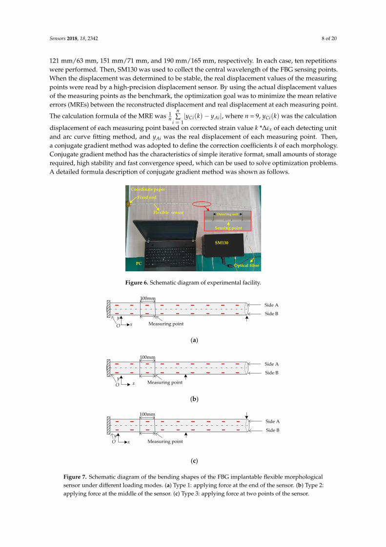
A morphological bending experiment was carried out in this study in order to verify the feasibilityof the morphological classification correction method, as shown in Figure 6. One end of the FBGimplantable flexible morphological sensor was fixed on the calibration platform with coordinate paper(cell: mm2). The coordinate of the fixed point on side B was O (0, 0), and the coordinates of eachmeasuring point on side B were Pj (100*j, 0), with j = 1, 2, . . . 9 (see Figure 7). On the other endof the sensor, the tail fiber was connected to the SM130, and the wavelength data of the two FBGarrays obtained by the SM130 demodulation were transmitted to the computer via a network cable.Then, displacements were applied to the different locations of the sensor for the formation of thedifferent bending shapes, and the displacements of each measuring point were read by a high-precisiondisplacement sensor (precision: 0.01 mm).

The experiment was conducted on three typical bending shapes of the FBG implantable flexiblemorphological sensors, as shown in Figure 7a–c, and six different sizes of displacement were applied toeach type. For Type 1 (Figure 7a), six different sizes of displacement were applied to the sensorat (900, 0) along the y direction, at 80 mm, 142 mm, 215 mm, 282 mm, 347 mm, and 400 mm,respectively. For Type 2 (Figure 7b), the displacements were applied along the y-axis at (500, 0)at 70 mm, 123 mm, 142 mm, 157 mm, 181 mm, and 211 mm, respectively. For Type 3 (Figure 7c), thedisplacements were applied to the sensor at (500, 0) and (900, 0) along the y direction, respectively,and the displacement values in the six cases were 50 mm/17 mm, 97 mm/49 mm, 96 mm/42 mm,

Sensors 2018, 18, 2342 8 of 20

121 mm/63 mm, 151 mm/71 mm, and 190 mm/165 mm, respectively. In each case, ten repetitionswere performed. Then, SM130 was used to collect the central wavelength of the FBG sensing points.When the displacement was determined to be stable, the real displacement values of the measuringpoints were read by a high-precision displacement sensor. By using the actual displacement valuesof the measuring points as the benchmark, the optimization goal was to minimize the mean relativeerrors (MREs) between the reconstructed displacement and real displacement at each measuring point.

The calculation formula of the MRE was 1n

n∑

i = 1|yCi(k)− yAi|, where n = 9, yCi(k) was the calculation

displacement of each measuring point based on corrected strain value k *∆εx of each detecting unitand arc curve fitting method, and yAi was the real displacement of each measuring point. Then,a conjugate gradient method was adopted to define the correction coefficients k of each morphology.Conjugate gradient method has the characteristics of simple iterative format, small amounts of storagerequired, high stability and fast convergence speed, which can be used to solve optimization problems.A detailed formula description of conjugate gradient method was shown as follows.

Sensors 2018, 18, x FOR PEER REVIEW 8 of 21

Fixed end

Flexible sensor

PC

SM130

Coordinate paper

Optical fiber

Detecting unit

Sensing point

Figure 6. Schematic diagram of experimental facility.

Side A

Side B

O Measuring point

100mm

x

y

(a)

Side A

Side B

Measuring point

100mm

O xy

(b)

Side A

Side B

O Measuring point

100mm

x

y

(c)

Figure 7. Schematic diagram of the bending shapes of the FBG implantable flexible morphological

sensor under different loading modes. (a) Type 1: applying force at the end of the sensor. (b) Type 2:

applying force at the middle of the sensor. (c) Type 3: applying force at two points of the sensor.

The experiment was conducted on three typical bending shapes of the FBG implantable flexible

morphological sensors, as shown in Figure 7a–c, and six different sizes of displacement were applied

to each type. For Type 1 (Figure 7a), six different sizes of displacement were applied to the sensor at

(900, 0) along the y direction, at 80 mm, 142 mm, 215 mm, 282 mm, 347 mm, and 400 mm, respectively.

For Type 2 (Figure 7b), the displacements were applied along the y-axis at (500, 0) at 70 mm, 123 mm,

142 mm, 157 mm, 181 mm, and 211 mm, respectively. For Type 3 (Figure 7c), the displacements were

applied to the sensor at (500, 0) and (900, 0) along the y direction, respectively, and the displacement

values in the six cases were 50 mm/17 mm, 97 mm/49 mm, 96 mm/42 mm, 121 mm/63 mm, 151 mm/71

mm, and 190 mm/165 mm, respectively. In each case, ten repetitions were performed. Then, SM130

was used to collect the central wavelength of the FBG sensing points. When the displacement was

determined to be stable, the real displacement values of the measuring points were read by a high-

precision displacement sensor. By using the actual displacement values of the measuring points as

the benchmark, the optimization goal was to minimize the mean relative errors (MREs) between the

reconstructed displacement and real displacement at each measuring point. The calculation formula

Figure 6. Schematic diagram of experimental facility.

Sensors 2018, 18, x FOR PEER REVIEW 8 of 21

Fixed end

Flexible sensor

PC

SM130

Coordinate paper

Optical fiber

Detecting unit

Sensing point

Figure 6. Schematic diagram of experimental facility.

Side A

Side B

O Measuring point

100mm

x

y

(a)

Side A

Side B

Measuring point

100mm

O xy

(b)

Side A

Side B

O Measuring point

100mm

x

y

(c)

Figure 7. Schematic diagram of the bending shapes of the FBG implantable flexible morphological

sensor under different loading modes. (a) Type 1: applying force at the end of the sensor. (b) Type 2:

applying force at the middle of the sensor. (c) Type 3: applying force at two points of the sensor.

The experiment was conducted on three typical bending shapes of the FBG implantable flexible

morphological sensors, as shown in Figure 7a–c, and six different sizes of displacement were applied

to each type. For Type 1 (Figure 7a), six different sizes of displacement were applied to the sensor at

(900, 0) along the y direction, at 80 mm, 142 mm, 215 mm, 282 mm, 347 mm, and 400 mm, respectively.

For Type 2 (Figure 7b), the displacements were applied along the y-axis at (500, 0) at 70 mm, 123 mm,

142 mm, 157 mm, 181 mm, and 211 mm, respectively. For Type 3 (Figure 7c), the displacements were

applied to the sensor at (500, 0) and (900, 0) along the y direction, respectively, and the displacement

values in the six cases were 50 mm/17 mm, 97 mm/49 mm, 96 mm/42 mm, 121 mm/63 mm, 151 mm/71

mm, and 190 mm/165 mm, respectively. In each case, ten repetitions were performed. Then, SM130

was used to collect the central wavelength of the FBG sensing points. When the displacement was

determined to be stable, the real displacement values of the measuring points were read by a high-

precision displacement sensor. By using the actual displacement values of the measuring points as

the benchmark, the optimization goal was to minimize the mean relative errors (MREs) between the

reconstructed displacement and real displacement at each measuring point. The calculation formula

Figure 7. Schematic diagram of the bending shapes of the FBG implantable flexible morphologicalsensor under different loading modes. (a) Type 1: applying force at the end of the sensor. (b) Type 2:applying force at the middle of the sensor. (c) Type 3: applying force at two points of the sensor.

Sensors 2018, 18, 2342 9 of 20

The optimization problem was

min f (k) =1n

n

∑i = 1|yCi(k)− yAi|. (11)

The sequence {km} could be obtained by the following iterative format,

km+1 = km + αmdm, (12)

where dm could be expressed as follows:

dm =

{−g(km), m = 0−gm(km) + βmdm−1, m ≥ 1

, (13)

whereg(km) = ∇ f (km). (14)

αm was search step size, which obtained by satisfying the following weak Wolfe conditions,

f (km + αmdm)− f (km) ≤ δαmg(km)Tdm, (15)

g(km+1)Tdm ≥ σg(km)

Tdm, (16)

where 0 < δ ≤ σ < 1. βm was the scalar of the representation algorithm and PRP method was selectedin this paper, which could be expressed as follows:

βPRPm = g(km)

T f (km−1)/‖g(km−1)‖2. (17)

The correction coefficient k of each morphology was obtained by the conjugate gradient method(see Table 3). Correction coefficients for Types 1 and 2 were determined to be k1 = 1.45 and k2 = 1.80,respectively. For Types 3, the correction coefficients of the positive and negative strain values werek3

+ = 1.49 and k3− = 1.10, respectively. The unified correction coefficient was the average of k1, k2, k3

+,and k3

−, and denoted as k= 1.46. However, no other morphological experiments were carried out inthis study, due to the limitations of the yield strength of the flexible substrate, experimental conditions,and other factors. However, there were still sufficient results achieved to confirm the feasibility of theproposed correction method.

Table 3. Correction coefficients of each bending morphology.

Bending Shapes Correction Coefficient

Type 1 k1 = 1.45Type 2 k2 = 1.80Type 3 k3

+ = 1.49, k3− = 1.10

4. Correction Methods

The morphological sensing algorithm which was based on arc curve fitting has the ability toevaluate the shape of the FBG implantable flexible morphological sensor. Thus, it is able to evaluatethe overall displacement profiles of the structures to be measured. However, the following factors maycause large morphological sensing errors and affect the precision of the displacement measurements.First, during the sensor fabrication processes, curvature measurement errors at the FBG sensing pointsmay easily be caused due to the deviations when implanting the FBG into the substrate. Second, thecurvatures measured by the flexible sensor are discontinuous, which is caused by a certain intervalbetween the adjacent FBG sensing points. The curvatures of the FBG sensing points are used to replace

Sensors 2018, 18, 2342 10 of 20

the curvatures of the detecting units in the calculation process of the arc curve fitting algorithm, whichmay induce the measurement errors. Third, the morphological sensing method is the integration ofthe piece-wise detecting units, and the displacement errors of each segment will gradually accumulateto generate accumulated errors at the end of the sensor.

To further improve the measurement accuracy of the FBG implantable flexible morphologicalsensor, the different bending shapes of the sensor were automatically categorized using the intelligentclassification algorithm. By calibrating the typical bending shapes of the sensor, the correctioncoefficients of different shapes were determined, and the corresponding correction coefficients ofdifferent bending shapes was then selected automatically to correct the reconstructed shapes for thepurpose of minimizing the errors.

ELM algorithm was adopted to intelligently classify the bending shapes of the FBG implantableflexible morphological sensor in this research study. ELM is a novel intelligence optimizationalgorithm for single-hidden layer feedforward neural networks (SLFNs), which was proposed in2004 [27]. This algorithm randomly selects hidden nodes and analytically determines the outputweights of SLFNs. Compared with conventional popular learning algorithms, this algorithm hasthe characteristics of extremely fast learning speed, good generalization performance, and tuning offree parameters. A detailed formula description of ELM was presented in Ref. [28].

Define that there are N arbitrary distinct training samples (xi, yi) ∈ Rn × Rm, where x are thetraining inputs and y are the training targets. The function of ELM classifier with L hidden layerneurons and a sigmoid function g(x) is mathematically modeled as follows:

L

∑j = 1

β jg(aj, bj, xi) = yi, i = 1, 2, . . . , N., (18)

where β j is output weight matrix, aj is input weight matrix, bj is bias connecting the input neurons.According to any continuous probability distribution, aj,bj can be randomly generated. Therefore,

the Equation (18) can be written in the form of the following matrix.

Hβ = Y, (19)

where

H =

g(a1, b1, x1) · · · g(aL, bL, x1)...

. . ....

g(a1, b1, xN) · · · g(aL, bL, xL)

N×L

, (20)

β =

βY1...

βYL

L×m

and Y =

yY1...

yYN

N×m

, (21)

where H is the hidden layer output matrix of ELM.These training algorithms need to adjust the input weights and the hidden layer biases, and the

output weights can be given as follows:β = H†Y, (22)

where H† is the Moore–Penrose generalized inverse of matrix H.When HTH is nonsingular,

H† = (HTH)−1

HT , (23)

or when HHT is nonsingular,

H† = HT(HHT)−1

. (24)

Sensors 2018, 18, 2342 11 of 20

Therefore, the output function of ELM classifier can be shown as follows:

f (x) = h(x)H†Y. (25)

The steps of classification of the morphological correction method were presented as follows:Step 1: The central wavelengths of the two FBG arrays were obtained using an FBG demodulator,

and Equation (4) was used to convert the wavelength variations at the sensing point to the curvature ofdetecting unit. Then, based on an arc curve fitting method, the bending shapes of the FBG implantableflexible morphological sensor were first reconstructed.

Step 2: The sensor was calibrated in order to obtain the actual displacement of each measuringpoint in the typical bending shape. Then, a conjugate gradient method was applied to determine thecorrection coefficients k of the different bending shapes, with the actual displacement as the standard.

Step 3: The experimental process was completed on different bending shapes, and then Step 1was repeated. The displacement of the measuring point Pi along the y-axis was taken as the input.Meanwhile, different bending shape types were regarded as the output in order to train the ELMclassifier model.

Step 4: An ELM classifier was used to classify the bending shapes first reconstructed in Step 1.Then, the corrected strain value k *∆εx of each detecting unit determined in Step 2 was applied toreconstruct the bending shapes of the FBG implantable flexible morphological sensor in order to obtainan accurate bending shape. The specific process was shown in Figure 8.

Sensors 2018, 18, x FOR PEER REVIEW 12 of 21

Obtaining the wavelengths of FBG sensing points

Calculating curvatures based on the measured wavelengths

Reconstructing the bending shapes using arc curve fitting method

Start

Initial reconstruction of bending shape as input

Type of typical bending shape as output

ELM Classifier

Real displacement

Minimized the MREs based on conjugate gradient method

Correction Coefficients k

Reconstructed displacement

Determination of correction coefficients k

Bending shape

Corresponding correction coefficients k

Correcting the reconstructed shapes

End

Figure 8. Flow chart of classification morphological correction method based on ELM intelligent

algorithm.

5. Simulation Verification

In this study, a finite element method was applied to simulate the bending shapes of the FBG

implantable flexible morphological sensor, and to compare the morphological sensing effects which

had been obtained by the unified coefficient and classification coefficient corrections. First, a cylinder

model with a length of 900 mm and a diameter of 5 mm was established, as shown in Figure

9a1,b1,c1,d1,e1. The initial end center coordinates of the cylinder model was O (0, 0, 0), and the cylinder

model was divided into nine segments along the x-axis. Each segment was taken as a detecting unit

of the proposed FBG implantable flexible morphological sensor. The column material was ABS, and

its mechanical property parameters were shown in Table 4. In this study’s simulation, the cylinder

model had a total of 4379 meshes with minimum unit masses of 0.351. Then, with consideration given

to the geometrical nonlinearity of the material used in the simulation, an elastic model was selected.

Table 4. Mechanical property parameters of ABS materials.

Parameters Value

elasticity modulus 2.2GPa

shearing modulus 318.9MPa

mass density 1020Kg/m3

tensile strength 30MPa

Poisson ratio 0.394

Figure 8. Flow chart of classification morphological correction method based on ELMintelligent algorithm.

The above method was adopted for bending shape classification correction of the proposed FBGimplantable flexible morphological sensor, which had the ability to effectively reduce the displacementerrors of the measuring points caused by the sensor preparation errors, FBG network capacitylimitations, and other factors. Therefore, the classification morphological correction method proposedin this study displayed the ability to improve the intellisense displacement abilities of the FBG flexiblemorphological sensor.

Sensors 2018, 18, 2342 12 of 20

5. Simulation Verification

In this study, a finite element method was applied to simulate the bending shapes of the FBGimplantable flexible morphological sensor, and to compare the morphological sensing effects which hadbeen obtained by the unified coefficient and classification coefficient corrections. First, a cylinder modelwith a length of 900 mm and a diameter of 5 mm was established, as shown in Figure 9a1,b1,c1,d1,e1.The initial end center coordinates of the cylinder model was O (0, 0, 0), and the cylinder model wasdivided into nine segments along the x-axis. Each segment was taken as a detecting unit of theproposed FBG implantable flexible morphological sensor. The column material was ABS, and itsmechanical property parameters were shown in Table 4. In this study’s simulation, the cylinder modelhad a total of 4379 meshes with minimum unit masses of 0.351. Then, with consideration given to thegeometrical nonlinearity of the material used in the simulation, an elastic model was selected.

Table 4. Mechanical property parameters of ABS materials.

Parameters Value

elasticity modulus 2.2GPashearing modulus 318.9MPamass density 1020Kg/m3

tensile strength 30MPaPoisson ratio 0.394

A displacement constraint was fixed on one side of the cylinder model, and five differenttypes of displacement were applied in order to simulate five different typical bending shapes.For Type 1 (Figure 9a1), a 140 mm displacement was applied along the y-axis at (900, −2.5, 0) inthe cylinder model. For Type 2 (Figure 9b1), a 50 mm displacement was applied along the y-axisat (500, −2.5, 0). For Type 3 (Figure 9c1), 92 mm and 30 mm displacements were applied along they-axis at (500, −2.5, 0) and (900, −2.5, 0), respectively. For Type 4 (Figure 9d1), 30 mm, 9.5 mm, and40 mm displacements were applied along the y-axis at (300, −2.5, 0), (600, −2.5, 0), and (900, −2.5, 0),respectively. For Type 5 (Figure 9e1), 30.7 mm, 11 mm, 38 mm, and 18.2 mm displacements wereapplied along the y-axis at (300, −2.5, 0), (500, −2.5, 0), (700, −2.5, 0), and (900, −2.5, 0), respectively.For the five typical bending shapes, the strain value at i = 0, 1, ... 8 in the coordinate points of Si(50 + 100*i, −2.5, 0) were extracted from the cylinder model. Meanwhile, the displacement at j = 1, 2, ...9 in the coordinate points of Pj (100*j, −2.5, 0) were extracted as the standard displacement values.The strain values which had been extracted were used for the first reconstruction of the differentbending shapes of the cylinder model by arc curve fitting method, in order to obtain the displacementof the measuring points under different bending shapes, as shown in Figure 9a2,b2,c2,d2,e2. It wasobserved that, having been influenced by multiple factors (such as the accumulated errors of detectingunits), there were certain errors between the first reconstructed displacement and the simulateddisplacement. For Types 1 and 2, the relative errors of the measuring points away from the fixedend had gradually increased (with maximum errors of 12.36 mm and 16.66 mm, respectively), andboth were located at the ninth measuring point. This was determined to be due to the fact that thecylinder model had undergone uniaxial stress conditions for Types 1 and 2, and each measuring pointdisplayed the same displacement error direction. The displacement errors of the measuring pointstended to accumulate point by point. However, for Types 3, 4, and 5, the measuring points with themaximum relative errors were located in the fifth, third, and seventh points, with relative error valuesof 13.81 mm, 4.93 mm, and 3.79 mm, respectively. These results may be due to the fact that the cylindermodel had undergone multidirectional stress conditions for Types 3, 4, and 5, and the displacementerrors of the measuring points displayed the phenomena of positive and negative error offsets.

Sensors 2018, 18, 2342 13 of 20

Sensors 2018, 18, x FOR PEER REVIEW 13 of 21

0 1 2 3 4 5 6 7 8 9

0

20

40

60

80

100

120

140

160

Dis

pla

cem

ent

(mm

)

Measuring points

Before correction

Classification coefficient correction

Uniform coefficient correction

Actual values

x

y

zO

(a1) (a2)

0 1 2 3 4 5 6 7 8 9

0

20

40

60

80

100

Before correction

Classification correction

Unified correction

Actual values

Dis

pla

cem

ent

(mm

)

Measuring points

s

x

y

zO

(b1) (b2)

0 1 2 3 4 5 6 7 8 9

0

20

40

60

80

100

Before correction

Classification correction

Unified correction

Actual values

Dis

pla

cem

ent

(mm

)

Measuring points

x

y

zO

(c1) (c2)

0 1 2 3 4 5 6 7 8 9

0

10

20

30

40

50

Before correction

Classification correction

Uniform correction

Actual values

Dis

pla

cem

ent

(mm

)

Measuring points

x

y

zO

(d1) (d2)

Figure 9. Cont.

Sensors 2018, 18, 2342 14 of 20

Sensors 2018, 18, x FOR PEER REVIEW 14 of 21

0 1 2 3 4 5 6 7 8 9

0

10

20

30

40

Before correction

Classification correction

Unified correction

Actual values

Dis

pla

cem

ent

(mm

)

Measuring points

x

y

zO

(e1) (e2)

Figure 9. The simulation diagram of the bending shapes of the FBG implantable flexible

morphological sensor under different loading modes and displacement at measuring points were

obtained based on the arc curve fitting algorithm. (a1) Simulation of applying force at the end of the

model. (a2) Displacement comparison of measuring points at Type 1. (b1) Simulation of applying force

at the middle of the model. (b2) Displacement comparison of measuring points at Type 2. (c1)

Simulation of applying force at two points of the model. (c2) Displacement comparison of measuring

points at Type 3. (d1) Simulation of applying force at three points of the model. (d2) Displacement

comparison of measuring points at Type 4. (e1) Simulation of applying force at four points of the

model. (e2) Displacement comparison of measuring points at Type 5.

A displacement constraint was fixed on one side of the cylinder model, and five different types

of displacement were applied in order to simulate five different typical bending shapes. For Type 1

(Figure 9a1), a 140 mm displacement was applied along the y-axis at (900, −2.5, 0) in the cylinder

model. For Type 2 (Figure 9b1), a 50 mm displacement was applied along the y-axis at (500, −2.5, 0).

For Type 3 (Figure 9c1), 92 mm and 30 mm displacements were applied along the y-axis at (500,

−2.5, 0) and (900, −2.5, 0), respectively. For Type 4 (Figure 9d1), 30 mm, 9.5 mm, and 40 mm

displacements were applied along the y-axis at (300, −2.5, 0), (600, −2.5, 0), and (900, −2.5, 0),

respectively. For Type 5 (Figure 9e1), 30.7 mm, 11 mm, 38 mm, and 18.2 mm displacements were

applied along the y-axis at (300, −2.5, 0), (500, −2.5, 0), (700, −2.5, 0), and (900, −2.5, 0), respectively. For

the five typical bending shapes, the strain value at i = 0, 1, ... 8 in the coordinate points of Si (50

+ 100*i, −2.5, 0) were extracted from the cylinder model. Meanwhile, the displacement at j = 1, 2, ... 9

in the coordinate points of Pj (100*j, −2.5, 0) were extracted as the standard displacement values. The

strain values which had been extracted were used for the first reconstruction of the different bending

shapes of the cylinder model by arc curve fitting method, in order to obtain the displacement of the

measuring points under different bending shapes, as shown in Figure 9a2,b2,c2,d2,e2. It was observed

that, having been influenced by multiple factors (such as the accumulated errors of detecting units),

there were certain errors between the first reconstructed displacement and the simulated

displacement. For Types 1 and 2, the relative errors of the measuring points away from the fixed end

had gradually increased (with maximum errors of 12.36 mm and 16.66 mm, respectively), and both

were located at the ninth measuring point. This was determined to be due to the fact that the cylinder

model had undergone uniaxial stress conditions for Types 1 and 2, and each measuring point

displayed the same displacement error direction. The displacement errors of the measuring points

tended to accumulate point by point. However, for Types 3, 4, and 5, the measuring points with the

maximum relative errors were located in the fifth, third, and seventh points, with relative error values

of 13.81 mm, 4.93 mm, and 3.79 mm, respectively. These results may be due to the fact that the

cylinder model had undergone multidirectional stress conditions for Types 3, 4, and 5, and the

displacement errors of the measuring points displayed the phenomena of positive and negative error

offsets.

During this study’s experimental process, based on the actual applied displacement as the

benchmark, weighted corrections were conducted on the first reconstructed morphology. Then, a

Figure 9. The simulation diagram of the bending shapes of the FBG implantable flexible morphologicalsensor under different loading modes and displacement at measuring points were obtained based on thearc curve fitting algorithm. (a1) Simulation of applying force at the end of the model. (a2) Displacementcomparison of measuring points at Type 1. (b1) Simulation of applying force at the middle of the model.(b2) Displacement comparison of measuring points at Type 2. (c1) Simulation of applying force at twopoints of the model. (c2) Displacement comparison of measuring points at Type 3. (d1) Simulationof applying force at three points of the model. (d2) Displacement comparison of measuring points atType 4. (e1) Simulation of applying force at four points of the model. (e2) Displacement comparison ofmeasuring points at Type 5.

During this study’s experimental process, based on the actual applied displacement as thebenchmark, weighted corrections were conducted on the first reconstructed morphology. Then,a conjugate gradient method was adopted to define the correction coefficient of each morphology.As detailed in Table 5, correction coefficients for Types 1 and 2 were determined to be k1 = 1.15 andk2 = 1.25, respectively. For Types 3, 4, and 5, the correction coefficients of the extracted positive andnegative strain values were k3

+ = 1.15 and k3− = 1.17, k4

+ = 1.14, k4− = 1.18, k5

+ = 1.19, k5− = 1.21,

respectively. The unified correction coefficient was the average of k1, k2, k3+, k3

−, k4+, k4

−, k5+, and

k5−, and denoted as k= 1.18. Figure 10 shows the MREs of the sensing displacement of the cylindrical

model under the five bending shapes based on different correction methods. It was observed thatunder the different bending shapes, the MREs of the measuring points were significantly differentwhen the strain values in the center of the detecting units were corrected using the unified coefficients.For Types 1, 2, 3, and 4, the MREs of the corrected measuring points were determined to decline, ofwhich that of Type 3 displayed the minimum decline of 0.84 mm, while that of Type 1 displayed themaximum decline of 4.27 mm. For Type 5, the MREs had increased following the corrections of theunified coefficients. However, for the different bending shapes, the errors in the measuring pointswhich had been corrected by the different coefficients had obviously decreased. The MREs had beenreduced by 4.33 mm (Type 1), 7.78 mm (Type 2), 6.47 mm (Type 3), 1.18 mm (Type 4), and 1.03 mm(Type 5), respectively, after the classification corrections. These findings indicated that, when comparedwith the unified coefficient corrections, the classification corrections of the different bending shapeshad improved the measurement precision of the displacements, which confirmed that it was necessaryto use different coefficient corrections for the various bending shapes.

Sensors 2018, 18, 2342 15 of 20

Table 5. Correction coefficients of each bending morphology.

Bending Shapes Correction Coefficient

Type 1 k1 = 1.15Type 2 k2 = 1.25Type 3 k3

+ = 1.15, k3− = 1.17

Type 4 k4+ = 1.14, k4

− = 1.18Type 5 k5

+ = 1.19, k5− = 1.21

Sensors 2018, 18, x FOR PEER REVIEW 15 of 21

conjugate gradient method was adopted to define the correction coefficient of each morphology. As

detailed in Table 5, correction coefficients for Types 1 and 2 were determined to be k1 = 1.15 and k2 =

1.25, respectively. For Types 3, 4, and 5, the correction coefficients of the extracted positive and

negative strain values were k3+ = 1.15 and k3− = 1.17, k4+ = 1.14, k4− = 1.18, k5+ = 1.19, k5− = 1.21, respectively.

The unified correction coefficient was the average of k1, k2, k3+, k3−, k4+, k4−, k5+, and k5−, and denoted as

k = 1.18. Figure 10 shows the MREs of the sensing displacement of the cylindrical model under the

five bending shapes based on different correction methods. It was observed that under the different

bending shapes, the MREs of the measuring points were significantly different when the strain values

in the center of the detecting units were corrected using the unified coefficients. For Types 1, 2, 3, and

4, the MREs of the corrected measuring points were determined to decline, of which that of Type 3

displayed the minimum decline of 0.84 mm, while that of Type 1 displayed the maximum decline of

4.27 mm. For Type 5, the MREs had increased following the corrections of the unified coefficients.

However, for the different bending shapes, the errors in the measuring points which had been

corrected by the different coefficients had obviously decreased. The MREs had been reduced by 4.33

mm (Type 1), 7.78 mm (Type 2), 6.47 mm (Type 3), 1.18 mm (Type 4), and 1.03 mm (Type 5),

respectively, after the classification corrections. These findings indicated that, when compared with

the unified coefficient corrections, the classification corrections of the different bending shapes had

improved the measurement precision of the displacements, which confirmed that it was necessary to

use different coefficient corrections for the various bending shapes.

Table 5. Correction coefficients of each bending morphology.

Bending Shapes Correction Coefficient

Type 1 k1 = 1.15

Type 2 k2 = 1.25

Type 3 k3+ = 1.15, k3− = 1.17

Type 4 k4+ = 1.14, k4− = 1.18

Type 5 k5+ = 1.19, k5− = 1.21

Figure 10. Comparison of MREs based on different correction methods under five bending shapes.

6. Experimental Analysis

6.1. Morphological Classification Based on ELM Algorithm

In Section 3.2, morphological calibration experiment was conducted on three typical bending

shapes of the FBG implantable flexible morphological sensors. Six different sizes of displacement

were applied to each type, and ten repetitions were performed in each case. An arc curve fitting

algorithm was used to calculate the initial morphology of the FBG implantable flexible morphological

Figure 10. Comparison of MREs based on different correction methods under five bending shapes.

6. Experimental Analysis

6.1. Morphological Classification Based on ELM Algorithm

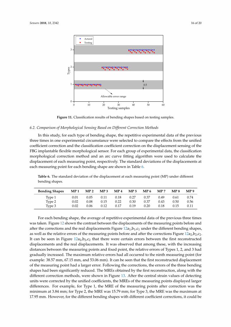
In Section 3.2, morphological calibration experiment was conducted on three typical bendingshapes of the FBG implantable flexible morphological sensors. Six different sizes of displacementwere applied to each type, and ten repetitions were performed in each case. An arc curve fittingalgorithm was used to calculate the initial morphology of the FBG implantable flexible morphologicalsensor. On this basis, an ELM algorithm was adopted to train the displacement data in the initialmorphology along the y direction. Also, the different bending shapes were intelligently classified.To be specific, for the six circumstances of each bending shape, the repetitive experimental data of theprevious seven times of each circumstance were taken as the training samples (training samples totaled126 groups). The displacement data of the training sample along the y-axis were used as the input,while the bending shape Types (Types 1, 2, and 3) were adopted as the output, in order to establish anELM model. The repetitive experimental data of the later three times were taken as the test samples(test samples totaled 54 groups) in order to verify the classification effects, and the results are shownin Figure 11. The classification intervals of Types 1, 2, and 3 were [0.75, 1.25], [1.75, 2.25], and [2.75,3.25], respectively. It was observed that for the 54 groups of test sample data, the ELM algorithm wasable to effectively realize the intelligent classification of the three typical bending shapes of the FBGimplantable flexible morphological sensor. The ELM algorithm was implemented based on MATLAprogramming software, with an entire program running time of 477 ms (computer configuration:Inter(R) Core(TM) i5-4210M CPU and 4G RAM). The results indicated that the algorithm had a fastcalculation speed with good generalization ability, and was able to effectively ensure the real-timeperformance of the morphological sensing.

Sensors 2018, 18, 2342 16 of 20

Sensors 2018, 18, x FOR PEER REVIEW 16 of 21

sensor. On this basis, an ELM algorithm was adopted to train the displacement data in the initial

morphology along the y direction. Also, the different bending shapes were intelligently classified. To

be specific, for the six circumstances of each bending shape, the repetitive experimental data of the

previous seven times of each circumstance were taken as the training samples (training samples

totaled 126 groups). The displacement data of the training sample along the y-axis were used as the

input, while the bending shape Types (Types 1, 2, and 3) were adopted as the output, in order to

establish an ELM model. The repetitive experimental data of the later three times were taken as the

test samples (test samples totaled 54 groups) in order to verify the classification effects, and the results

are shown in Figure 11. The classification intervals of Types 1, 2, and 3 were [0.75, 1.25], [1.75, 2.25],

and [2.75, 3.25], respectively. It was observed that for the 54 groups of test sample data, the ELM

algorithm was able to effectively realize the intelligent classification of the three typical bending

shapes of the FBG implantable flexible morphological sensor. The ELM algorithm was implemented

based on MATLA programming software, with an entire program running time of 477 ms (computer

configuration: Inter(R) Core(TM) i5-4210M CPU and 4G RAM). The results indicated that the

algorithm had a fast calculation speed with good generalization ability, and was able to effectively

ensure the real-time performance of the morphological sensing.

0 10 20 30 40 50 60

0

1

2

3

Allowable error range

Actural

Testing

Ty

pes

Testing samples

0.5

Figure 11. Classification results of bending shapes based on testing samples.

6.2. Comparison of Morphological Sensing Based on Different Correction Methods

In this study, for each type of bending shape, the repetitive experimental data of the previous

three times in one experimental circumstance were selected to compare the effects from the unified

coefficient correction and the classification coefficient correction on the displacement sensing of the

FBG implantable flexible morphological sensor. For each group of experimental data, the

classification morphological correction method and an arc curve fitting algorithm were used to

calculate the displacement of each measuring point, respectively. The standard deviations of the

displacements at each measuring point for each bending shape are shown in Table 6.

Table 6. The standard deviation of the displacement at each measuring point (MP) under different

bending shapes.

Bending Shapes MP 1 MP 2 MP 3 MP 4 MP 5 MP 6 MP 7 MP 8 MP 9

Type 1 0.01 0.05 0.11 0.18 0.27 0.37 0.49 0.61 0.74

Type 2 0.02 0.08 0.15 0.22 0.30 0.37 0.43 0.50 0.56

Type 3 0.02 0.06 0.12 0.17 0.19 0.20 0.18 0.15 0.11

For each bending shape, the average of repetitive experimental data of the previous three times

was taken. Figure 12 shown the contrast between the displacements of the measuring points before

Figure 11. Classification results of bending shapes based on testing samples.

6.2. Comparison of Morphological Sensing Based on Different Correction Methods

In this study, for each type of bending shape, the repetitive experimental data of the previousthree times in one experimental circumstance were selected to compare the effects from the unifiedcoefficient correction and the classification coefficient correction on the displacement sensing of theFBG implantable flexible morphological sensor. For each group of experimental data, the classificationmorphological correction method and an arc curve fitting algorithm were used to calculate thedisplacement of each measuring point, respectively. The standard deviations of the displacements ateach measuring point for each bending shape are shown in Table 6.

Table 6. The standard deviation of the displacement at each measuring point (MP) under differentbending shapes.

Bending Shapes MP 1 MP 2 MP 3 MP 4 MP 5 MP 6 MP 7 MP 8 MP 9

Type 1 0.01 0.05 0.11 0.18 0.27 0.37 0.49 0.61 0.74Type 2 0.02 0.08 0.15 0.22 0.30 0.37 0.43 0.50 0.56Type 3 0.02 0.06 0.12 0.17 0.19 0.20 0.18 0.15 0.11

For each bending shape, the average of repetitive experimental data of the previous three timeswas taken. Figure 12 shown the contrast between the displacements of the measuring points before andafter the corrections and the real displacements Figure 12a1,b1,c1 under the different bending shapes,as well as the relative errors of the measuring points before and after the corrections Figure 12a2,b2,c2.It can be seen in Figure 12a2,b2,c2 that there were certain errors between the first reconstructeddisplacements and the real displacements. It was observed that among these, with the increasingdistances between the measuring points and fixed point, the relative errors of Types 1, 2, and 3 hadgradually increased. The maximum relative errors had all occurred to the ninth measuring point (forexample: 38.57 mm, 67.15 mm, and 53.06 mm). It can be seen that the first reconstructed displacementof the measuring point had a larger error. Following the corrections, the errors of the three bendingshapes had been significantly reduced. The MREs obtained by the first reconstruction, along with thedifferent correction methods, were shown in Figure 13. After the central strain values of detectingunits were corrected by the unified coefficients, the MREs of the measuring points displayed largerdifferences. For example, for Type 1, the MRE of the measuring points after correction was theminimum at 3.84 mm; for Type 2, the MRE was 15.79 mm; for Type 3, the MRE was the maximum at17.95 mm. However, for the different bending shapes with different coefficient corrections, it could be

Sensors 2018, 18, 2342 17 of 20

seen that the MREs of measuring points had obviously decreased. The MREs of Types 1, 2, and 3 afterthe classification corrections were 4.8 mm, 1.67 mm, and 2.4 mm, respectively. The MREs had beenreduced by 13.16 mm (Type 1), 29.90 mm (Type 2), and 30.56 mm (Type 3), respectively, following theclassification corrections. When compared with the unified coefficient corrections, the classificationcoefficient corrections displayed a good correction ability for the displacement errors of the measuringpoints with different bending shapes.

Sensors 2018, 18, x FOR PEER REVIEW 17 of 21

and after the corrections and the real displacements Figure 12a1,b1,c1 under the different bending

shapes, as well as the relative errors of the measuring points before and after the corrections Figure

12a2,b2,c2. It can be seen in Figure 12a2,b2,c2 that there were certain errors between the first

reconstructed displacements and the real displacements. It was observed that among these, with the

increasing distances between the measuring points and fixed point, the relative errors of Types 1, 2,

and 3 had gradually increased. The maximum relative errors had all occurred to the ninth measuring

point (for example: 38.57 mm, 67.15 mm, and 53.06 mm). It can be seen that the first reconstructed

displacement of the measuring point had a larger error. Following the corrections, the errors of the

three bending shapes had been significantly reduced. The MREs obtained by the first reconstruction,

along with the different correction methods, were shown in Figure 13. After the central strain values

of detecting units were corrected by the unified coefficients, the MREs of the measuring points

displayed larger differences. For example, for Type 1, the MRE of the measuring points after

correction was the minimum at 3.84 mm; for Type 2, the MRE was 15.79 mm; for Type 3, the MRE

was the maximum at 17.95 mm. However, for the different bending shapes with different coefficient

corrections, it could be seen that the MREs of measuring points had obviously decreased. The MREs

of Types 1, 2, and 3 after the classification corrections were 4.8 mm, 1.67 mm, and 2.4 mm, respectively.

The MREs had been reduced by 13.16 mm (Type 1), 29.90 mm (Type 2), and 30.56 mm (Type 3),

respectively, following the classification corrections. When compared with the unified coefficient

corrections, the classification coefficient corrections displayed a good correction ability for the

displacement errors of the measuring points with different bending shapes.

0 1 2 3 4 5 6 7 8 9

0

20

40

60

80

100

120

140

160

Before correction

Classification correction

Unified correction

Actual values

Dis

pla

cem

ent

(mm

)

Measuring points

1 2 3 4 5 6 7 8 90

10

20

30

40

50

Rel

ativ

e er

rors

(m

m)

Measuring points

Classification correction

Unified correction

Before correction

(a1) (a2)

0 1 2 3 4 5 6 7 8 9

0

20

40

60

80

100

120

140 Before correction

Classification correction

Unified correction

Actual values

Dis

pla

cem

ent

(mm

)

Measuring points

1 2 3 4 5 6 7 8 90

20

40

60

80

100

120

Classification correction

Unified correction

Before correction

Rel

ativ

e er

rors

(m

m)

Measuring points (b1) (b2)

Sensors 2018, 18, x FOR PEER REVIEW 18 of 21

0 1 2 3 4 5 6 7 8 9 10

0

20

40

60

80

100

Before correction

Classification correction

Uniform correction

Actual values

Dis

pla

cem

ent

(mm

)

Measuring points

1 2 3 4 5 6 7 8 90

20

40

60

80

100

120

Classification correction

Unified correction

Before correction

Rel

ativ

e er

rors

(m

m)

Measuring points (c1) (c2)

Figure 12. Demonstration of experimental results under three bending shapes of FBG implantable

flexible morphological sensor. (a1) Displacement comparison of measuring points at Type 1. (a2)

Relative errors comparison of measuring points at Type 1. (b1) Displacement comparison of

measuring points at Type 2. (b2) Relative errors comparison of measuring points at Type 2. (c1)

Displacement comparison of measuring points at Type 3. (c2) Relative errors comparison of measuring

points at Type 3.

Figure 13. Comparison of mean relative errors (MREs) based on different methods under three

bending shapes.

Table 7 shows the relative error percentages at each measuring point under the three bending

shapes following the classification corrections. It could be seen that under the different bending

shapes, the maximum relative error percentages of each measuring point of the FBG implantable

flexible morphological sensor were 6.39% (Type 1), 7.04% (Type 2), and 7.02% (Type 3), respectively.

Following the corrections of the different bending shapes, the relative error percentages of each

measuring point were observed to be relatively low. These findings indicated that the proposed

classification morphological correction method was feasible, and the method was found to effective

in improving the precision of the FBG implantable flexible morphological sensor when sensing

deformation fields in geotechnical engineering related applications.

Figure 12. Demonstration of experimental results under three bending shapes of FBG implantableflexible morphological sensor. (a1) Displacement comparison of measuring points at Type 1.(a2) Relative errors comparison of measuring points at Type 1. (b1) Displacement comparisonof measuring points at Type 2. (b2) Relative errors comparison of measuring points at Type 2.(c1) Displacement comparison of measuring points at Type 3. (c2) Relative errors comparison ofmeasuring points at Type 3.

Sensors 2018, 18, 2342 18 of 20

Sensors 2018, 18, x FOR PEER REVIEW 18 of 21

0 1 2 3 4 5 6 7 8 9 10

0

20

40

60

80

100

Before correction

Classification correction

Uniform correction

Actual values

Dis

pla

cem

ent

(mm

)

Measuring points

1 2 3 4 5 6 7 8 90

20

40

60

80

100

120

Classification correction

Unified correction

Before correction

Rel

ativ

e er

rors

(m

m)

Measuring points (c1) (c2)

Figure 12. Demonstration of experimental results under three bending shapes of FBG implantable

flexible morphological sensor. (a1) Displacement comparison of measuring points at Type 1. (a2)

Relative errors comparison of measuring points at Type 1. (b1) Displacement comparison of

measuring points at Type 2. (b2) Relative errors comparison of measuring points at Type 2. (c1)

Displacement comparison of measuring points at Type 3. (c2) Relative errors comparison of measuring

points at Type 3.

Figure 13. Comparison of mean relative errors (MREs) based on different methods under three

bending shapes.

Table 7 shows the relative error percentages at each measuring point under the three bending

shapes following the classification corrections. It could be seen that under the different bending

shapes, the maximum relative error percentages of each measuring point of the FBG implantable

flexible morphological sensor were 6.39% (Type 1), 7.04% (Type 2), and 7.02% (Type 3), respectively.

Following the corrections of the different bending shapes, the relative error percentages of each

measuring point were observed to be relatively low. These findings indicated that the proposed

classification morphological correction method was feasible, and the method was found to effective

in improving the precision of the FBG implantable flexible morphological sensor when sensing

deformation fields in geotechnical engineering related applications.

Figure 13. Comparison of mean relative errors (MREs) based on different methods under threebending shapes.

Table 7 shows the relative error percentages at each measuring point under the three bendingshapes following the classification corrections. It could be seen that under the different bendingshapes, the maximum relative error percentages of each measuring point of the FBG implantableflexible morphological sensor were 6.39% (Type 1), 7.04% (Type 2), and 7.02% (Type 3), respectively.Following the corrections of the different bending shapes, the relative error percentages of eachmeasuring point were observed to be relatively low. These findings indicated that the proposedclassification morphological correction method was feasible, and the method was found to effectivein improving the precision of the FBG implantable flexible morphological sensor when sensingdeformation fields in geotechnical engineering related applications.

Table 7. The relative error percentages of the displacements at each measuring point (MP) afterclassification correction.

Bending Shapes MP 1 MP 2 MP 3 MP 4 MP 5 MP 6 MP 7 MP 8 MP 9

Type 1 3.43 3.00 4.90 4.52 6.39 5.38 5.16 5.68 4.68Type 2 2.02 1.94 3.92 5.27 3.21 2.03 3.16 4.67 7.04Type 3 1.04 5.86 7.02 3.76 2.38 0.35 1.66 4.15 6.74

7. Conclusions

In this research, an FBG implantable flexible morphological sensor with the capacityof temperature self-compensation, bending shape self-classification, and displacement errorself-correction was designed by internally implanting a 180◦ spacing FBG array in an ABS rod. Onthis basis, the causes of the morphological sensing errors were analyzed for an FBG implantableflexible morphological sensor. Meanwhile, the key focus was to propose a morphological sensingmethod for an FBG implantable flexible sensor based on classification morphological corrections.A temperature calibration experiment was performed to verify that the influences of temperaturecould be eliminated by using the central wavelength variations of two FBG sensing points in eachdetecting unit. Although limited by such factors as the yielding strength of the flexible rod substrateand various experimental conditions, this study’s experiments were carried out on three typicalbending shapes of the FBG implantable flexible morphological sensor, and the correction coefficients kof each morphology were obtained by the conjugate gradient method. A finite element simulation wasadopted for five typical bending shapes of a cylinder model, and the necessity and feasibility of the

Sensors 2018, 18, 2342 19 of 20

proposed method were analyzed. The intelligent classification of the different bending shapes wererealized using an ELM classifier. During this study’s experimental process, the MREs of the measuringpoints were observed to be significantly reduced following the coefficient corrections of the differentbending shapes. The MREs were found to be reduced by 13.16 mm (Type 1), 29.90 mm (Type 2), and30.56 mm (Type 3), respectively, following the classification corrections. When compared with theunified coefficient corrections, the classification coefficient corrections displayed a good correctionability for the displacement errors at the measuring points in the different bending shapes. Followingthe corrections by the classification morphological correction method, the maximum relative errorpercentages of the displacements at measuring points in different bending shapes were determinedto be 6.39% (Type 1), 7.04% (Type 2), and 7.02% (Type 3), respectively. Following the corrections ofthe different bending shapes, the relative error percentages of each of the measuring points wererelatively low. These findings confirmed that the proposed classification correction method wasfeasible and effective in improving the intelligent displacement sensing ability of the FBG implantableflexible morphological sensor. However, due to the limitations of the experimental conditions andthe properties of the substrate material, the experimental validation was only carried out on threemorphologies in this study. In the future, the correction performances of various bending shapes willbe considered in detail, and the effects of the proposed classification morphological correction methodunder three-dimensional coordinates will be further examined. This study’s designed FBG implantableflexible morphological sensor can be potentially used for the real-time monitoring of deformationfields in rock masses, subgrades, bridges, as well as other geotechnical engineering processes, andpresents vital significance and application promotion value.

Author Contributions: Conceptualization, Z.W. and J.W.; Data curation, C.T. and Z.W.; Formal analysis, C.T.;Investigation, C.T. and Q.S.; Software, Y.D., Y.L. and M.H.; Supervision, L.J. and H.W.; Validation, C.T. and Y.D.;Writing—original draft, C.T.

Funding: This research was funded by the National Natural Science Foundation of China (41602292 and 41472260);The Fundamental Research Funds of Shandong University (2017TB008); The National Major Scientific InstrumentDevelopment Project of China (51427804); Major scientific and technological innovation projects of ShandongProvince (2017CXGC0610).

Conflicts of Interest: The authors declare no conflict of interest.

References

1. Roesthuis, R.J.; Kemp, M.; van den Dobbelsteen, J.J.; Misra, S. Three-Dimensional needle shape reconstructionusing an array of Fiber Bragg Grating sensors. IEEE/ASME Trans. Mechatron. 2014, 19, 1115–1126. [CrossRef]

2. Zhu, H.H.; Yin, J.H.; Zhang, L.; Jin, W.; Dong, J.H. Monitoring internal displacements of a model dam usingFBG sensing bars. Adv. Struct. Eng. 2010, 13, 249–261. [CrossRef]

3. Kefal, A.; Yildiz, M. Modeling of sensor placement strategy for shape sensing and structural healthmonitoring of a wing-shaped sandwich panel using inverse finite element method. Sensors 2017, 17, 2775.[CrossRef] [PubMed]

4. Wang, H.S.; Zhang, R.X.; Chen, W.D.; Liang, X.W.; Pfeifer, R. Shape detection algorithm for soft manipulatorbased on Fiber Bragg Gratings. IEEE/ASME Trans. Mechatron. 2016, 21, 2977–2982. [CrossRef]

5. Kim, H.I.; Kang, L.H.; Han, J.H. Shape estimation with distributed fiber Bragg grating sensors for rotatingstructures. Smart Mater. Struct. 2011, 20, 035011. [CrossRef]

6. Pei, H.F.; Yin, J.H.; Zhu, H.H.; Hong, C.Y.; Jin, W.; Xu, D.S. Monitoring of lateral displacements of a slopeusing a series of special fiber Bragg grating-based in-place inclinometers. Meas. Sci. Technol. 2012, 23, 025007.[CrossRef]

7. Bang, H.J.; Kim, H.I.; Lee, K.S. Measurement of strain and bending deflection of a wind turbine tower usingarrayed FBG sensors. Int. J. Precis. Eng. Manuf. 2012, 13, 2121–2126. [CrossRef]

8. Rapp, S.; Kang, L.H.; Han, J.H.; Mueller, U.C.; Baier, H. Displacement field estimation for a two-dimensionalstructure using fiber Bragg grating sensors. Smart Mater. Struct. 2009, 18, 025006. [CrossRef]

9. Payo, I.; Feliu, V.; Cortazar, O.D. Fibre Bragg grating (FBG) sensor system for highly flexible single-linkrobots. Sens. Actuators A Phys. 2009, 150, 24–39. [CrossRef]

Sensors 2018, 18, 2342 20 of 20

10. Xu, L.; Ge, J.; Patel, J.H.; Fork, M.P. Dual-layer orthogonal fiber Bragg grating mesh based soft sensor for3-dimensional shape sensing. Opt. Express 2017, 25, 24727–24734. [CrossRef] [PubMed]

11. Bhamber, R.S.; Allsop, T.; Lloyd, G.; Webb, D.J.; Ania-Castanon, J.D. Arbitrary real-time three-dimensionalcorporal object sensing and reconstruction scheme. Opt. Lett. 2012, 37, 3549–3551. [CrossRef] [PubMed]

12. Yi, J.C.; Zhu, X.J.; Zhang, H.S.; Shen, L.Y.; Qiao, X.P. Spatial shape reconstruction using orthogonal fiberBragg grating sensor array. Mechatronics 2012, 22, 679–687. [CrossRef]

13. Kang, L.H.; Kim, D.K.; Han, J.H. Estimation of dynamic structural displacements using fiber Bragg gratingstrain sensors. J. Sound Vib. 2007, 305, 534–542. [CrossRef]

14. Todd, M.D.; Stull, C.J.; Dickerson, M. A locally-exact strain-to-displacement approach for shapereconstruction of slender objects using fiber Bragg gratings. In Proceedings of the Smart Sensor Phenomena,Technology, Networks, and Systems Integration, San Diego, CA, USA, 10–14 March 2013.

15. Li, Y.; Wang, H.P.; Zhu, W.S.; Li, S.C.; Liu, J. Structural stability monitoring of a physical model test onan underground cavern group during deep excavations using FBG sensors. Sensors 2015, 15, 21696–21709.[CrossRef] [PubMed]

16. Guo, Y.X.; Zhang, D.S.; Fu, J.J.; Liu, S.B.; Zhang, S.Z.; Zhu, F.D. Development and operation of a fiber Bragggrating based online monitoring strategy for slope deformation. Sens. Rev. 2015, 35, 348–356. [CrossRef]

17. Kim, N.S.; Cho, N.S. Estimating deflection of a simple beam model using fiber optic Bragg-grating sensors.Exp. Mech. 2004, 44, 433–439. [CrossRef]

18. Xu, H.; Ren, W.X.; Wang, Z.C. Deflection estimation of bending beam structures using fiber Bragg gratingstrain sensors. Adv. Struct. Eng. 2015, 18, 395–403. [CrossRef]

19. Zhang, H.S.; Zhu, X.J.; Gao, Z.Y.; Liu, K.N.; Li, Z.W. Dynamic error analysis method for vibration shapereconstruction of smart FBG plate structure. Shock Vib. 2016, 2016, 5958073. [CrossRef]

20. Sun, G.; Li, H.; Dong, M.L.; Lou, X.P.; Zhu, L.Q. Optical fiber shape sensing of polyimide skin for a flexiblemorphing wing. Appl. Opt. 2017, 56, 9325–9332. [CrossRef] [PubMed]

21. Wang, Z.F.; Wang, J.; Sui, Q.M.; Jia, L.; Li, S.C.; Liang, X.M.; Lu, S.D. Deformation reconstruction of a smartGeogrid embedded with fiber Bragg grating sensors. Meas. Sci. Technol. 2015, 26, 125202. [CrossRef]

22. Wang, Z.F.; Wang, J.; Sui, Q.M.; Li, S.C.; Jia, L. In-situ calibrated deformation reconstruction method for fiberBragg grating embedded smart Geogrid. Sens. Actuators A Phys. 2016, 250, 145–158. [CrossRef]

23. Kinet, D.; Mégret, P.; Goossen, K.W.; Qiu, L.; Heider, D.; Caucheteur, C. Fiber Bragg grating sensors towardstructural health monitoring in composite materials: Challenges and solutions. Sensors 2014, 14, 7394–7419.[CrossRef] [PubMed]

24. Mishra, V.; Singh, N.; Tiwari, U.; Kapur, P. Fiber grating sensors in medicine: Current and emergingapplications. Sens. Actuators A Phys. 2011, 167, 279–290. [CrossRef]

25. Ge, J.; James, A.E.; Xu, L.; Chen, Y.; Kwok, K.W.; Fok, M.P. Bidirectional soft silicone curvature sensor basedon off-centered embedded fiber Bragg grating. IEEE Photonics Technol. Lett. 2016, 28, 2237–2240. [CrossRef]

26. Boresi, A.P.; Richard, J.S. Advanced Mechanics of Materials, 6th ed.; Wiley: San Francisco, CA, USA, 2002;pp. 263–294, ISBN 978-0-471-43881-6.

27. Huang, G.B.; Zhu, Q.Y.; Siew, C.K. Extreme learning machine: A new learning scheme of feedforwardneural networks. In Proceedings of the IEEE International Joint Conference on Neural Networks, Budapest,Hungary, 25–29 July 2004.

28. Huang, G.B.; Zhu, Q.Y.; Siew, C.K. Extreme learning machine: Theory and applications. Neurocomputing2006, 70, 489–501. [CrossRef]

© 2018 by the authors. Licensee MDPI, Basel, Switzerland. This article is an open accessarticle distributed under the terms and conditions of the Creative Commons Attribution(CC BY) license (http://creativecommons.org/licenses/by/4.0/).