design and evaluation of a distributed control ... · design and evaluation of a distributed...
TRANSCRIPT
ISSN 0280-5316 ISRN LUTFD2/TFRT--5878--SE
Design and evaluation of a distributed control architecture over switched
Ethernet in active filters
Erik Hansson Martin Sträng
Department of Automatic Control Lund University
March 2011


Lund University Department of Automatic Control Box 118 SE-221 00 Lund Sweden
Document name
MASTER THESIS Date of issue
March 2011 Document Number
ISRN LUTFD2/TFRT--5878--SE Author(s)
Erik Hansson and Martin Sträng
Supervisor
Jonas Persson Comsys AB Lund, Sweden Karl-Erik Årzén Automatic Control Lund, Sweden (Examiner) Sponsoring organization
Title and subtitle
Design and evaluation of a distributed control architecture over switched Ethernet in active filters. (Design och utvärdering av en switchad Ethernet arkitektur för aktiva filter)
Abstract
The area of power quality has received more and more attention during the last decade. Poor power quality is a growing problem, especially for the industry because it has a negative effect on production efficiency, power consumption and equipment life-span. Active filters are one of the more widespread solutions to these problems. An active filter is often sized and installed to compensate a specific load, based on a preceding power quality measurement. Often one system is not enough and multiple parallel systems must be used. This thesis investigates if it is possible to design a distributed control system where a number of filters work together and communicate using a switched Ethernet network. Such a distributed system can offer advantages such as better coordination and simplified configuration and operation. In the resulting distributed system the control tasks are split into two groups, power quality controllers and hardware controllers. The power quality controllers are executed by a master control computer and the resulting setpoint is distributed through the network to a number of slaves. The distributed system has been tested both through simulations and in a real-world implementation. Based on these tests it can be concluded that the distributed system works and that its performance is only marginally affected compared to the original system.
Keywords
Classification system and/or index terms (if any)
Supplementary bibliographical information
ISSN and key title
0280-5316 ISBN
Language
English Number of pages
67 Recipient’s notes
Security classification
http://www.control.lth.se/publications/


Preface
We would like to thank Comsys AB and especially our supervisor Jonas Persson for making this thesis
work possible. We would also like to thank Nils Lundström for taking time to answer our questions
and to help us in the lab. Lastly we would like to thank Prof. Karl-Erik Årzén for his excellent
support.
CONTENTS CONTENTS
Contents1 Introduction 6
1.1 The ADF P300 . . . . . . . . . . . . . . . . . . . . . . . . . . . . . . . . . . . . . 6
1.2 Purpose . . . . . . . . . . . . . . . . . . . . . . . . . . . . . . . . . . . . . . . . . 7
1.3 Motivation . . . . . . . . . . . . . . . . . . . . . . . . . . . . . . . . . . . . . . . . 8
1.4 Report outline . . . . . . . . . . . . . . . . . . . . . . . . . . . . . . . . . . . . . . 8
1.5 Division of work . . . . . . . . . . . . . . . . . . . . . . . . . . . . . . . . . . . . 9
2 Three phase systems 102.1 Three phase theory . . . . . . . . . . . . . . . . . . . . . . . . . . . . . . . . . . . 10
2.1.1 Positive and negative sequences . . . . . . . . . . . . . . . . . . . . . . . . 10
2.1.2 αβ-transform . . . . . . . . . . . . . . . . . . . . . . . . . . . . . . . . . . 11
2.1.3 dq-transform . . . . . . . . . . . . . . . . . . . . . . . . . . . . . . . . . . 11
2.2 Power quality issues . . . . . . . . . . . . . . . . . . . . . . . . . . . . . . . . . . . 12
2.2.1 Reactive power . . . . . . . . . . . . . . . . . . . . . . . . . . . . . . . . . 12
2.2.2 Harmonics . . . . . . . . . . . . . . . . . . . . . . . . . . . . . . . . . . . 13
2.2.3 Flicker . . . . . . . . . . . . . . . . . . . . . . . . . . . . . . . . . . . . . 13
2.2.4 Unbalance . . . . . . . . . . . . . . . . . . . . . . . . . . . . . . . . . . . 14
2.3 Active filters . . . . . . . . . . . . . . . . . . . . . . . . . . . . . . . . . . . . . . . 14
3 Ethernet 153.1 Standard Ethernet . . . . . . . . . . . . . . . . . . . . . . . . . . . . . . . . . . . . 15
3.1.1 Ethernet evolution . . . . . . . . . . . . . . . . . . . . . . . . . . . . . . . 15
3.1.2 The Ethernet Frame . . . . . . . . . . . . . . . . . . . . . . . . . . . . . . . 15
3.1.3 PAUSE Control frame . . . . . . . . . . . . . . . . . . . . . . . . . . . . . 16
3.2 Industrial Ethernet . . . . . . . . . . . . . . . . . . . . . . . . . . . . . . . . . . . 17
3.3 Latency in a switched network . . . . . . . . . . . . . . . . . . . . . . . . . . . . . 17
3.4 Switched Fast Ethernet . . . . . . . . . . . . . . . . . . . . . . . . . . . . . . . . . 19
3.4.1 Theoretical example . . . . . . . . . . . . . . . . . . . . . . . . . . . . . . 19
3.5 Summary . . . . . . . . . . . . . . . . . . . . . . . . . . . . . . . . . . . . . . . . 20
4 Study of Ethernet in the SCC2 214.1 Measured transfer time . . . . . . . . . . . . . . . . . . . . . . . . . . . . . . . . . 21
4.1.1 Crossover cable . . . . . . . . . . . . . . . . . . . . . . . . . . . . . . . . . 21
4.1.2 One switch . . . . . . . . . . . . . . . . . . . . . . . . . . . . . . . . . . . 22
4.1.3 Two switches . . . . . . . . . . . . . . . . . . . . . . . . . . . . . . . . . . 23
4.1.4 One sender and two mirrors . . . . . . . . . . . . . . . . . . . . . . . . . . 24
4.1.5 Switch fabric time . . . . . . . . . . . . . . . . . . . . . . . . . . . . . . . 25
4.1.6 Lost frames . . . . . . . . . . . . . . . . . . . . . . . . . . . . . . . . . . . 25
4.2 Ethernet driver performance . . . . . . . . . . . . . . . . . . . . . . . . . . . . . . 26
4.3 Interaction between the Ethernet driver and the control loop . . . . . . . . . . . . . . 26
4.4 Summary . . . . . . . . . . . . . . . . . . . . . . . . . . . . . . . . . . . . . . . . 27
5 Control architecture in the ADF 285.1 General control structure . . . . . . . . . . . . . . . . . . . . . . . . . . . . . . . . 28
CONTENTS CONTENTS
5.2 ADF system controllers . . . . . . . . . . . . . . . . . . . . . . . . . . . . . . . . . 29
5.2.1 UDC . . . . . . . . . . . . . . . . . . . . . . . . . . . . . . . . . . . . . . 29
5.2.2 Current control . . . . . . . . . . . . . . . . . . . . . . . . . . . . . . . . . 29
5.3 Power quality controllers . . . . . . . . . . . . . . . . . . . . . . . . . . . . . . . . 30
5.3.1 Harmonics . . . . . . . . . . . . . . . . . . . . . . . . . . . . . . . . . . . 30
5.3.2 Reactive power . . . . . . . . . . . . . . . . . . . . . . . . . . . . . . . . . 31
5.3.3 Unbalance . . . . . . . . . . . . . . . . . . . . . . . . . . . . . . . . . . . 31
5.3.4 Flicker . . . . . . . . . . . . . . . . . . . . . . . . . . . . . . . . . . . . . 31
5.4 Identified requirements . . . . . . . . . . . . . . . . . . . . . . . . . . . . . . . . . 32
5.5 Test case . . . . . . . . . . . . . . . . . . . . . . . . . . . . . . . . . . . . . . . . . 32
5.6 Summary . . . . . . . . . . . . . . . . . . . . . . . . . . . . . . . . . . . . . . . . 32
6 A distributed control architecture 346.1 Design . . . . . . . . . . . . . . . . . . . . . . . . . . . . . . . . . . . . . . . . . . 34
6.1.1 Motivation . . . . . . . . . . . . . . . . . . . . . . . . . . . . . . . . . . . 35
6.2 Simulation tools . . . . . . . . . . . . . . . . . . . . . . . . . . . . . . . . . . . . . 35
6.2.1 Simulink model . . . . . . . . . . . . . . . . . . . . . . . . . . . . . . . . . 35
6.2.2 Using TrueTime to simulate network transfer . . . . . . . . . . . . . . . . . 36
6.3 Experimental setup . . . . . . . . . . . . . . . . . . . . . . . . . . . . . . . . . . . 37
6.3.1 Test loads . . . . . . . . . . . . . . . . . . . . . . . . . . . . . . . . . . . . 37
6.3.2 Monitored signals . . . . . . . . . . . . . . . . . . . . . . . . . . . . . . . 39
6.3.3 Sampling . . . . . . . . . . . . . . . . . . . . . . . . . . . . . . . . . . . . 40
6.4 A first attempt . . . . . . . . . . . . . . . . . . . . . . . . . . . . . . . . . . . . . . 40
6.4.1 Results . . . . . . . . . . . . . . . . . . . . . . . . . . . . . . . . . . . . . 41
6.4.2 Analysis . . . . . . . . . . . . . . . . . . . . . . . . . . . . . . . . . . . . 43
6.5 A better approach . . . . . . . . . . . . . . . . . . . . . . . . . . . . . . . . . . . . 44
6.5.1 Results . . . . . . . . . . . . . . . . . . . . . . . . . . . . . . . . . . . . . 46
6.5.2 Analysis . . . . . . . . . . . . . . . . . . . . . . . . . . . . . . . . . . . . 48
6.6 Summary . . . . . . . . . . . . . . . . . . . . . . . . . . . . . . . . . . . . . . . . 48
7 Implementation of the distributed architecture 507.1 Scope of the implementation . . . . . . . . . . . . . . . . . . . . . . . . . . . . . . 50
7.2 Implementation . . . . . . . . . . . . . . . . . . . . . . . . . . . . . . . . . . . . . 50
7.2.1 Concurrency issues . . . . . . . . . . . . . . . . . . . . . . . . . . . . . . . 52
7.2.2 Find master algorithm . . . . . . . . . . . . . . . . . . . . . . . . . . . . . 53
7.2.3 Retransmission . . . . . . . . . . . . . . . . . . . . . . . . . . . . . . . . . 53
7.2.4 Error handling . . . . . . . . . . . . . . . . . . . . . . . . . . . . . . . . . 54
7.2.5 Message types . . . . . . . . . . . . . . . . . . . . . . . . . . . . . . . . . 54
7.3 Summary . . . . . . . . . . . . . . . . . . . . . . . . . . . . . . . . . . . . . . . . 55
8 Testing of the distributed architecture 568.1 Hardware setup . . . . . . . . . . . . . . . . . . . . . . . . . . . . . . . . . . . . . 56
8.2 ADF Settings . . . . . . . . . . . . . . . . . . . . . . . . . . . . . . . . . . . . . . 57
8.3 Test loads . . . . . . . . . . . . . . . . . . . . . . . . . . . . . . . . . . . . . . . . 57
8.4 Measurements . . . . . . . . . . . . . . . . . . . . . . . . . . . . . . . . . . . . . . 59
8.5 Results . . . . . . . . . . . . . . . . . . . . . . . . . . . . . . . . . . . . . . . . . . 59

CONTENTS CONTENTS
8.5.1 Step response rectifier load . . . . . . . . . . . . . . . . . . . . . . . . . . . 60
8.5.2 Step response capacitor load . . . . . . . . . . . . . . . . . . . . . . . . . . 61
8.5.3 Steady state . . . . . . . . . . . . . . . . . . . . . . . . . . . . . . . . . . . 62
8.6 Analysis . . . . . . . . . . . . . . . . . . . . . . . . . . . . . . . . . . . . . . . . . 63
8.7 Summary . . . . . . . . . . . . . . . . . . . . . . . . . . . . . . . . . . . . . . . . 64
9 Discussion and conclusion 65
Nomenclature
AC Alternating Current
ADF Active Dynamic Filter
CRC Cyclic Redundancy Check
DC Direct Current
DMA Direct Memory Access
DSP Digital Signal Processor
FFT Fast Fourier Transform
FPGA Field Programmable Gate Array
IGBT Insulated-Gate Bipolar Transistor
MAC Media Access Control
PP Power Processor
PWM Pulse Width Modulation
RMS Root Mean Square
1 INTRODUCTION
1 Introduction
Comsys AB was founded in 1996 with the vision to provide the knowledge and equipment needed to
help clients optimize their energy consumption. The company headquarter is located in Lund in close
proximity to Lund university. Comsys develops and manufactures solutions for improving power
quality in industrial environments. The term power quality is often used as a unification that refers
to all disturbances that cause deviations from a pure sinus waveform in an Alternating Current (AC)
system. Such disturbances can cause problems like lower performance, downtime in production,
shorter life span of equipment [17] and excessive power usage [6].
One method to overcome these power quality issues is to install some type of filter. There are many
kinds of filters on the market but they can in general be divided into two groups, active and passive
filters. Comsys main product line consist of active filters called Active Dynamic Filter (ADF) and
there are several different models. The main difference between the models is their compensation
current capacity. To find out what capacity is needed in a specific case, measurements that record
the behaviour of the disturbing loads are performed. Based on these measurements it is possible to
calculate how many ADFs that are needed to rectify the measured problems. This means that it is a
common case that more than one ADF is running in parallel.
1.1 The ADF P300
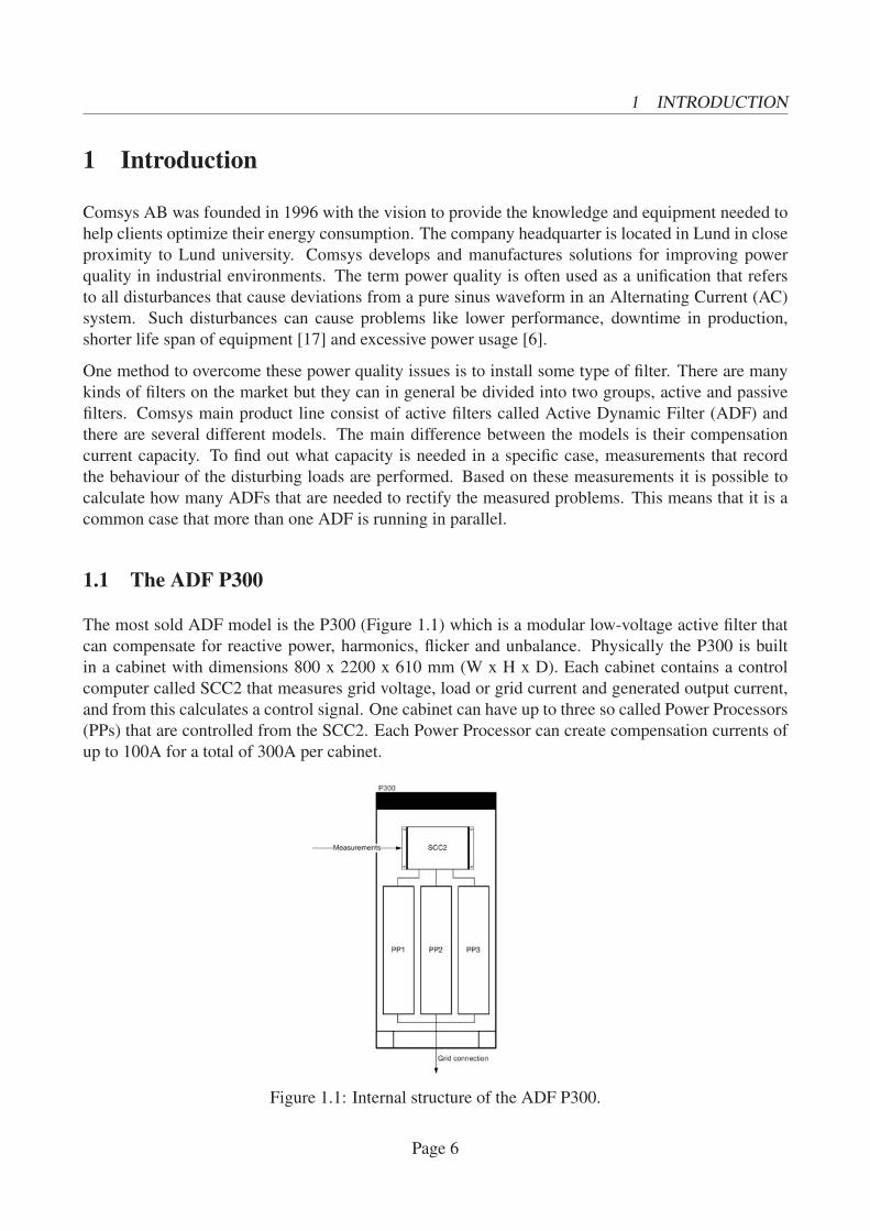
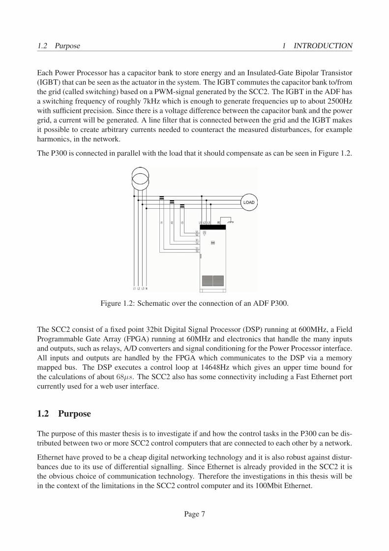
The most sold ADF model is the P300 (Figure 1.1) which is a modular low-voltage active filter that
can compensate for reactive power, harmonics, flicker and unbalance. Physically the P300 is built
in a cabinet with dimensions 800 x 2200 x 610 mm (W x H x D). Each cabinet contains a control
computer called SCC2 that measures grid voltage, load or grid current and generated output current,
and from this calculates a control signal. One cabinet can have up to three so called Power Processors
(PPs) that are controlled from the SCC2. Each Power Processor can create compensation currents of
up to 100A for a total of 300A per cabinet.
Figure 1.1: Internal structure of the ADF P300.
Page 6
1.2 Purpose 1 INTRODUCTION
Each Power Processor has a capacitor bank to store energy and an Insulated-Gate Bipolar Transistor
(IGBT) that can be seen as the actuator in the system. The IGBT commutes the capacitor bank to/from
the grid (called switching) based on a PWM-signal generated by the SCC2. The IGBT in the ADF has
a switching frequency of roughly 7kHz which is enough to generate frequencies up to about 2500Hz
with sufficient precision. Since there is a voltage difference between the capacitor bank and the power
grid, a current will be generated. A line filter that is connected between the grid and the IGBT makes
it possible to create arbitrary currents needed to counteract the measured disturbances, for example
harmonics, in the network.
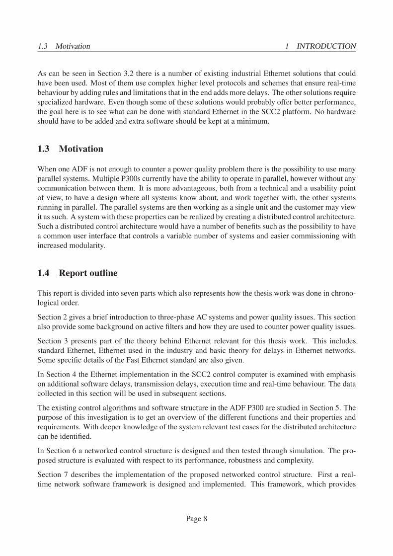
The P300 is connected in parallel with the load that it should compensate as can be seen in Figure 1.2.
Figure 1.2: Schematic over the connection of an ADF P300.
The SCC2 consist of a fixed point 32bit Digital Signal Processor (DSP) running at 600MHz, a Field
Programmable Gate Array (FPGA) running at 60MHz and electronics that handle the many inputs
and outputs, such as relays, A/D converters and signal conditioning for the Power Processor interface.
All inputs and outputs are handled by the FPGA which communicates to the DSP via a memory
mapped bus. The DSP executes a control loop at 14648Hz which gives an upper time bound for
the calculations of about 68μs. The SCC2 also has some connectivity including a Fast Ethernet port
currently used for a web user interface.
1.2 Purpose
The purpose of this master thesis is to investigate if and how the control tasks in the P300 can be dis-
tributed between two or more SCC2 control computers that are connected to each other by a network.
Ethernet have proved to be a cheap digital networking technology and it is also robust against distur-
bances due to its use of differential signalling. Since Ethernet is already provided in the SCC2 it is
the obvious choice of communication technology. Therefore the investigations in this thesis will be
in the context of the limitations in the SCC2 control computer and its 100Mbit Ethernet.
Page 7
1.3 Motivation 1 INTRODUCTION
As can be seen in Section 3.2 there is a number of existing industrial Ethernet solutions that could
have been used. Most of them use complex higher level protocols and schemes that ensure real-time
behaviour by adding rules and limitations that in the end adds more delays. The other solutions require
specialized hardware. Even though some of these solutions would probably offer better performance,
the goal here is to see what can be done with standard Ethernet in the SCC2 platform. No hardware
should have to be added and extra software should be kept at a minimum.
1.3 Motivation
When one ADF is not enough to counter a power quality problem there is the possibility to use many
parallel systems. Multiple P300s currently have the ability to operate in parallel, however without any
communication between them. It is more advantageous, both from a technical and a usability point
of view, to have a design where all systems know about, and work together with, the other systems
running in parallel. The parallel systems are then working as a single unit and the customer may view
it as such. A system with these properties can be realized by creating a distributed control architecture.
Such a distributed control architecture would have a number of benefits such as the possibility to have
a common user interface that controls a variable number of systems and easier commissioning with
increased modularity.
1.4 Report outline
This report is divided into seven parts which also represents how the thesis work was done in chrono-
logical order.
Section 2 gives a brief introduction to three-phase AC systems and power quality issues. This section
also provide some background on active filters and how they are used to counter power quality issues.
Section 3 presents part of the theory behind Ethernet relevant for this thesis work. This includes
standard Ethernet, Ethernet used in the industry and basic theory for delays in Ethernet networks.
Some specific details of the Fast Ethernet standard are also given.
In Section 4 the Ethernet implementation in the SCC2 control computer is examined with emphasis
on additional software delays, transmission delays, execution time and real-time behaviour. The data
collected in this section will be used in subsequent sections.
The existing control algorithms and software structure in the ADF P300 are studied in Section 5. The
purpose of this investigation is to get an overview of the different functions and their properties and
requirements. With deeper knowledge of the system relevant test cases for the distributed architecture
can be identified.
In Section 6 a networked control structure is designed and then tested through simulation. The pro-
posed structure is evaluated with respect to its performance, robustness and complexity.
Section 7 describes the implementation of the proposed networked control structure. First a real-
time network software framework is designed and implemented. This framework, which provides
Page 8

1.5 Division of work 1 INTRODUCTION
an abstraction layer that hides all the details associated with network transmission, is then used to
implement the distributed control system.
In Section 8 the implemented system is tested and evaluated using similar strategies as in the simula-
tions.
1.5 Division of work
Erik Hansson studied the control architecture in the ADF (Section 5) and made the design for the
distributed control system (Section 6).
Martin Sträng studied the Ethernet implementation in the given platform (Section 4) and implemented
the real-world test system (Section 7)
Testing of the real world implementation in Section 8 was done by both Martin and Erik.
Page 9
2 THREE PHASE SYSTEMS
2 Three phase systems
This section provides a brief background to three phase systems and surrounding terminology used
in this thesis. Also mathematical tools needed in the analysis of three phase systems are introduced.
This includes the αβ and dq transform and sequence representation. Different power quality issues
are described and the advantages of active filters compared to passive solutions are presented.
2.1 Three phase theory
In an ideal three phase system all phases have equal amplitude and all the phases have a phase differ-
ence of 120◦. Such a system is said to be symmetric or balanced [14]. If the first phase (a) is used
as a reference then the second phase (b) lags the first phase by 120◦ and the third phase (c) lags the
second phase also by 120◦ as in Equation 2.1.
⎧⎨⎩
Va(t) = Va cos(2πf · t)Vb(t) = Vb cos(2πf · t− 2π/3)Vc(t) = Vc cos(2πf · t− 4π/3)
(2.1)
In a balanced three phase system the sum of the phase voltages are always zero as in Equation 2.2.
Va(t) + Vb(t) + Vc(t) = 0 (2.2)
2.1.1 Positive and negative sequences
When phase b lags phase a by 120◦ the phases are said to have a positive sequence. If it is phase c that
lags phase a by 120◦ the phases are said to have a negative sequence and the voltages are described
by Equation 2.3.
⎧⎨⎩
Va(t) = Va cos(2πf · t)Vb(t) = Vb cos(2πf · t− 4π/3)Vc(t) = Vc cos(2πf · t− 2π/3)
(2.3)
A unbalanced three phase system can be represented as a sum (Equation 2.4) of positive and negative
sequence components where the positive and negative sequence components are balanced.
⎡⎣ Va(t)
Vb(t)Vc(t)
⎤⎦ =
⎡⎣ Vp cos(2πf · t)
Vp cos(2πf · t− 2π/3)Vp cos(2πf · t− 4π/3)
⎤⎦+
⎡⎣ Vn cos(2πf · t)
Vn cos(2πf · t− 4π/3)Vn cos(2πf · t− 2π/3)
⎤⎦ (2.4)
To transform from abc to sequence components Equation 2.5 is used.
Page 10

2.1 Three phase theory 2 THREE PHASE SYSTEMS
[Vp
Vn
]=
1
3
[1 a a2
1 a2 a
]⎡⎣ Va
Vb
Vc
⎤⎦ (2.5)
Transformation in the opposite direction is done using Equation 2.6
⎡⎣ Va
Vb
Vc
⎤⎦ =
⎡⎣ 1 1
a2 aa a2
⎤⎦[Vp
Vn
](2.6)
where a = ej2π3 .
2.1.2 αβ-transform
If a three phase system is balanced, that is Equation 2.2 holds, the system describing the phase volt-
ages or currents is over-determined [14]. A consequence of this is that such a three phase system can
be transformed into an equivalent two phase system, which is more convenient to work with. This
transformation is called the αβ or the Clarke transform and its matrix representation is presented in
Equation 2.7 and 2.8.
[Xα
Xβ
]=
√2
3
[1 −1/2 −1/2
0√3/2 −√
3/2
]⎡⎣ Xa
Xb
Xc
⎤⎦ (2.7)
⎡⎣ Xa
Xb
Xc
⎤⎦ =
√2
3
⎡⎣ 1 0
−1/2√3/2
−1/2 −√3/2
⎤⎦[Xα
Xβ
](2.8)
where X∗ could be voltages or currents.
2.1.3 dq-transform
The analysis of three phase systems can be simplified even further with the use of yet another trans-
formation. The dq-transformation takes a rotating vector in αβ coordinates and expresses it as a
stationary vector in a rotating reference frame. This means that analysis can be done on DC-level
voltages and currents instead of oscillating such [14]. Transformation from αβ coordinates to dq
coordinates and back is expressed in Equation 2.9 and 2.10 [7]:
[Xd
Xq
]=
[cos(ωt) sin(ωt)−sin(ωt) cos(ωt)
] [Xα
Xβ
](2.9)
[Xα
Xβ
]=
[cos(ωt) −sin(ωt)sin(ωt) cos(ωt)
] [Xd
Xq
](2.10)
Page 11

2.2 Power quality issues 2 THREE PHASE SYSTEMS
where ω is the angular velocity of the original three phase signal. Another convenient fact is that in
dq coordinates, d represents the reactive part and q the active part of the voltage or current [14].
From now on the notation dqX will be used to indicate the use of a coordinate system rotating with
the frequency of X Hz. The addition neg is used to indicate negative sequence. For example, dq250
refers to a positive sequence system rotating with 250 Hz.
2.2 Power quality issues
Most of the equipment connected to the electrical power grid is designed to use a power supply with
certain predefined characteristics such as voltage and frequency. It is of high importance that the grid
can deliver a voltage that meet this specification. Variations or deviations will have a negative effect
on reliability, efficiency and equipment life-span and are thus highly unwanted.
Below is a short description of the most common types of power quality issues.
Figure 2.1: Conceptual illustration of power quality issues.
2.2.1 Reactive power
The total power consumed by a load connected to an AC power grid is called the apparent power and
is denoted S:
S = Urms · Irms
S can be divided into two parts, active and reactive power. The active power (P) represents power that
can be converted to useful work, for example the mechanical force produced by an electric motor.
Reactive power (Q) on the other hand is the result of inductances and capacitances in the grid and
load. It does no useful work but is still necessary for example to generate the required magnetic flux
in the same electric motor.
Considering only the base grid frequency from now on, active and reactive power can be calculated
using
P = S cos(ϕ) = UrmsIrms cos(ϕ)
Q = S sin(ϕ) = UrmsIrms sin(ϕ)
where ϕ is the phase difference between the voltage and current (see Figure 2.1) [6].
Page 12

2.2 Power quality issues 2 THREE PHASE SYSTEMS
The power factor
PF =P
S=
P√P 2 +Q2
= cosϕ
provides information about the proportion of active power with respect to the apparent power. For
example a power factor of 1 indicates that the load is purely resistive, that is, there is no reactive
power.
Although reactive power is necessary in many applications it is wasteful to transfer this energy back
and forth across the power grid. This is mainly due to the fact that this reactive power occupies grid
capacity that could otherwise have been used to transfer active power. Even though reactive power
does not transfer any net energy in any direction it still contributes to the total current flowing in the
power lines which in the end increases losses due to grid impedance.
2.2.2 Harmonics
Harmonics are voltages or currents with other frequencies than the fundamental that exist in the
electric grid. Harmonics are usually multiples of the fundamental frequency and they are caused
by non-linear devices which create non sinusoidal currents because the relationship between voltage
and current is not constant during a set period of time [17]. The largest source of harmonics are
semiconductors. Common loads that have this behaviour are: rectifiers and electric arc furnaces in
the industry and fluorescent lamps, switched mode power supplies and other electronic devices in a
home environment. An example of a fundamental with superimposed fifth harmonic can be seen in
Figure 2.1.
The harmonic load currents will result in a similar voltage-drop, creating corresponding harmonics in
the voltage. If the grid is weak these voltage harmonics may propagate out onto the electric grid and
create problems at other places. The harmonics can then be considerably amplified due to resonances
between inductances and capacitances in the grid.
High levels of harmonics can cause many different problems, for example: increased losses in ca-
bles and equipment [18], noise and incorrect operation of machines leading do increased wear and
premature failure and cause disturbances in electronic equipment [17].
2.2.3 Flicker
Some large power hungry industrial loads such as welding machines and electric arc furnaces give
rise to fast asynchronous variations in the rms grid voltage [17]. These voltage variations are usually
not a problem for other loads but may be disturbing to human beings because they can for example
cause lights to flicker. When the voltage variations (or a combination of higher frequency variations)
are in the frequency range 1-30Hz (and especially around 9Hz) the flicker has been found to be the
most disturbing to human beings [6].
Page 13
2.3 Active filters 2 THREE PHASE SYSTEMS
2.2.4 Unbalance
In a three phase symmetric power system all the voltages have equal amplitude and the phase angle
between all the phases are equal. If the voltages do not have these properties the voltages are said
to be unbalanced (Figure2.1). Problems with unbalanced three phase voltages are usually a result of
single phase loads [17]. Unbalanced three phase systems can cause overload in for example variable
speed drives and lowered efficiency of induction motors. Variable speed drives may also generate an
increased amount of harmonics when connected to an unbalanced three phase network.
2.3 Active filters
There are basically two solutions to the power quality situations mentioned above. Either the equip-
ment connected to the electrical power grid is designed in such a way that it can tolerate the above
disturbances (load conditioning) or specialized conditioning equipment is installed to counteract the
disturbances [9].
The second alternative, called Energy Conditioners, has proven to be an efficient way of getting rid
of the most harmful disturbances. There are many different types of energy conditioners but they can
generally be divided into passive and active filters. Passive filters have to be designed to fit the load
that they are supposed to compensate [10]. They also must be switched on or off depending on if
the load is running or not, since they otherwise can generate disturbances themselves. In a factory
with many different loads it is very hard to design passive filters that work well for all possible load
conditions.
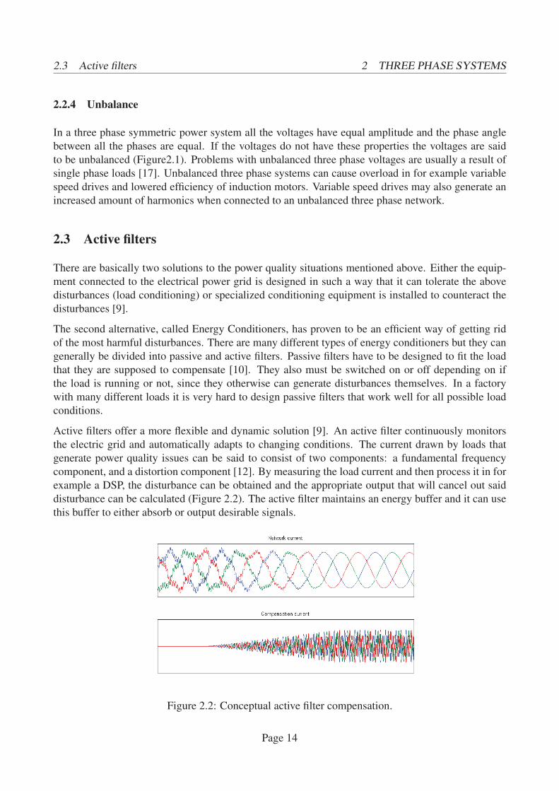
Active filters offer a more flexible and dynamic solution [9]. An active filter continuously monitors
the electric grid and automatically adapts to changing conditions. The current drawn by loads that
generate power quality issues can be said to consist of two components: a fundamental frequency
component, and a distortion component [12]. By measuring the load current and then process it in for
example a DSP, the disturbance can be obtained and the appropriate output that will cancel out said
disturbance can be calculated (Figure 2.2). The active filter maintains an energy buffer and it can use
this buffer to either absorb or output desirable signals.
Figure 2.2: Conceptual active filter compensation.
Page 14
3 ETHERNET
3 Ethernet
In this section the Ethernet networking technology will be examined from the aspect of industrial
applications. First a brief summary of the Ethernet evolution will be presented. Then some insight
in existing industrial Ethernet solutions will be given. Lastly the properties and performance of Fast
Ethernet will be examined.
3.1 Standard Ethernet
Ethernet has been around since 1976 and has gone through four generations ranging from the first
10Mbps version to the still not so widely used 10Gbps version [16]. It was standardized 1983 in
IEEE 802.3. Ethernet is today the most widely used LAN technology in homes and workplaces, and
is also taking ground in industrial environments.
3.1.1 Ethernet evolution
Throughout the evolution of Ethernet a number of different physical and logical topologies have been
used [8]. Among the first were the bus and the hubbed star networks. In the bus variant each station
is tapped in to one cable and the whole cable represents the collision domain. This means that all
stations connected to the same network share the same medium and will have to use a shared access
protocol (CSMA/CD in Ethernet) to avoid data loss due to collisions. In the hubbed star network
each station is connected to a central point, the hub. The hub is a multi-port repeater that broadcasts
incoming frames to all ports. The collision domain is still the entire network.
Obviously problems will arise when a collision domain grows too large. The network bandwidth is
shared among all stations in a collision domain. When the number of stations grow, performance and
reliability will drop fast. The solution to this problem is to use a network bridge to separate network
segments. This will have two major impacts on network performance: The bandwidth is no longer
shared by all stations in the network but by the stations in the same segment. Also, each segment now
represents its own collision domain.
The next evolutionary step is to replace the hub with a switch. A switch can be seen as a multi-
port bridge and thus each port on the switch represents its own network and collision domain. Now
collisions can only happen if a station and the switch should send at the same time. By going one step
further and using full duplex switched Ethernet collisions can no longer happen and there is no need
for the CSMA/CD mechanism.
The CSMA/CD and its non-determinism was one of the properties of Ethernet making it unsuitable
for real-time applications. With that out of the way the one remaining obstacle is buffering [15].
3.1.2 The Ethernet Frame
Data sent through an Ethernet network is divided into frames. Each frame is handled separately and
there is no acknowledging mechanism. This is of benefit for real-time applications since retrans-
Page 15
3.1 Standard Ethernet 3 ETHERNET
mission of lost data units often is not the desirable behaviour and it would be a waste of time and
resources to force this functionality. If the application requires reliable transmissions, functionality
will have to be added in upper layers.
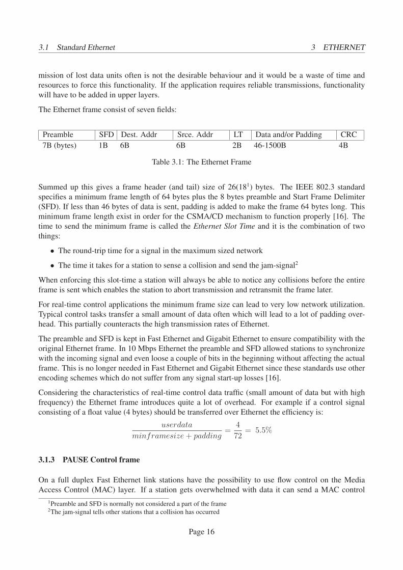
The Ethernet frame consist of seven fields:
Preamble SFD Dest. Addr Srce. Addr LT Data and/or Padding CRC
7B (bytes) 1B 6B 6B 2B 46-1500B 4B
Table 3.1: The Ethernet Frame
Summed up this gives a frame header (and tail) size of 26(181) bytes. The IEEE 802.3 standard
specifies a minimum frame length of 64 bytes plus the 8 bytes preamble and Start Frame Delimiter
(SFD). If less than 46 bytes of data is sent, padding is added to make the frame 64 bytes long. This
minimum frame length exist in order for the CSMA/CD mechanism to function properly [16]. The
time to send the minimum frame is called the Ethernet Slot Time and it is the combination of two
things:
• The round-trip time for a signal in the maximum sized network
• The time it takes for a station to sense a collision and send the jam-signal2
When enforcing this slot-time a station will always be able to notice any collisions before the entire
frame is sent which enables the station to abort transmission and retransmit the frame later.
For real-time control applications the minimum frame size can lead to very low network utilization.
Typical control tasks transfer a small amount of data often which will lead to a lot of padding over-
head. This partially counteracts the high transmission rates of Ethernet.
The preamble and SFD is kept in Fast Ethernet and Gigabit Ethernet to ensure compatibility with the
original Ethernet frame. In 10 Mbps Ethernet the preamble and SFD allowed stations to synchronize
with the incoming signal and even loose a couple of bits in the beginning without affecting the actual
frame. This is no longer needed in Fast Ethernet and Gigabit Ethernet since these standards use other
encoding schemes which do not suffer from any signal start-up losses [16].
Considering the characteristics of real-time control data traffic (small amount of data but with high
frequency) the Ethernet frame introduces quite a lot of overhead. For example if a control signal
consisting of a float value (4 bytes) should be transferred over Ethernet the efficiency is:
userdata
minframesize+ padding=
4
72= 5.5%
3.1.3 PAUSE Control frame
On a full duplex Fast Ethernet link stations have the possibility to use flow control on the Media
Access Control (MAC) layer. If a station gets overwhelmed with data it can send a MAC control
1Preamble and SFD is normally not considered a part of the frame2The jam-signal tells other stations that a collision has occurred
Page 16
3.2 Industrial Ethernet 3 ETHERNET
frame with the PAUSE command, requesting the sender to wait for a specified time before resuming
transmission. The MAC control features are optional [16] and should typically be turned off in a real
time application.
3.2 Industrial Ethernet
Traditionally the industry has been using a plethora of proprietary network solutions and protocols
which often require expensive specialized hardware and software licences. Different manufacturers
often use different technologies which leads to a lot of problems, if not making it impossible, when
trying to integrate these systems. Also many of these technologies offer low performance and complex
implementations. Since most industries nowadays use PCs and other computer equipment that need
to be networked it is not unusual that one site has two or three different networks.
Development of new, high performing solutions is expensive and also requires expert knowledge in
the field. Since Ethernet is a well proven, standardized and high performing technology it has seen
more and more use in the industry [4].
There exist a number of industrial Ethernet network solutions developed by some of the larger in-
dustrial organizations. They have diverging specializations but share the basic idea of making use of
Ethernet’s strengths and avoiding its shortcomings in supporting real time applications. Common for
all Ethernet solutions is that they add functionality, either in software or hardware, to ensure real-time
behaviour and increase performance.
EtherCat [1] and SERCOS III [3] are two examples of industrial Ethernet networks that require
specialized hardware, like a FPGA, to handle network traffic. EtherCat nodes have two network ports
that allow them to read frames without having to receive and store them. This means that frames can
pass through nodes with almost no delay. Since data for different nodes reside in the same frames the
efficiency can be very high.
FL-Net, Modbus-TCP/IDA, ProfiNet-IO, Ethernet/IP and Ethernet Powerlink use the TCP/IP or
UDP/IP protocol stack and adds protocols on higher layers in the OSI stack to get the desired real-time
deterministic behaviour [2]. This of course adds computing overhead and delays to the transmissions.
Industrial Ethernet have a number of benefits over most proprietary industrial networks. These include
greater bandwidth, short delays, increased distance, better interoperability and the use of cheap and
available standard equipment. Unfortunately there are also some downsides such as low efficiency
due to the minimum frame size and the lack of determinism.
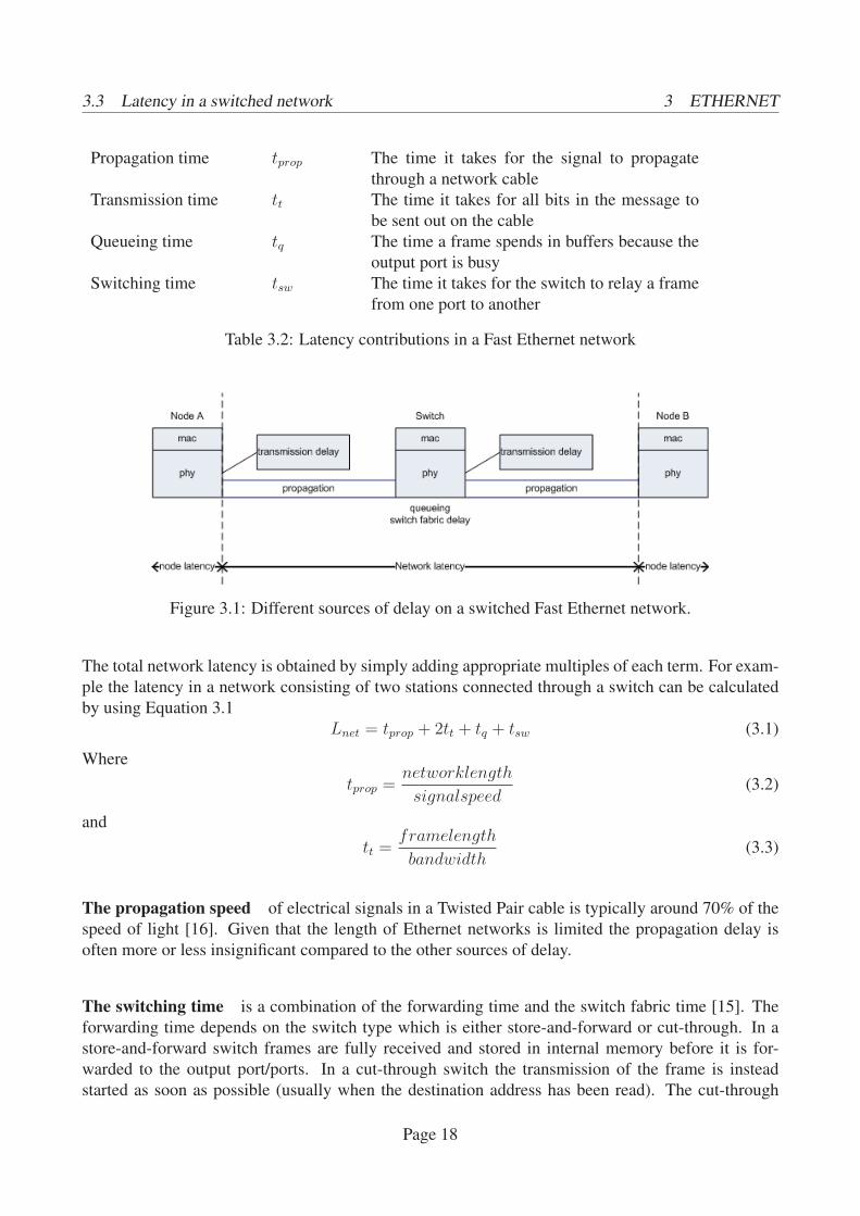
3.3 Latency in a switched network
The Network Latency is the time between when the first bit is sent out on the network until the frame
is completely received at the destination. The Network Latency consist of the four terms listed in
Table 3.2 [8]. The Network Latency only includes the delays originating from the network itself. It
does not cover delays in the sending or receiving node. An illustration of this can be seen in Figure 3.1.
Page 17
3.3 Latency in a switched network 3 ETHERNET
Propagation time tprop The time it takes for the signal to propagate
through a network cable
Transmission time tt The time it takes for all bits in the message to
be sent out on the cable
Queueing time tq The time a frame spends in buffers because the
output port is busy
Switching time tsw The time it takes for the switch to relay a frame
from one port to another
Table 3.2: Latency contributions in a Fast Ethernet network
Figure 3.1: Different sources of delay on a switched Fast Ethernet network.
The total network latency is obtained by simply adding appropriate multiples of each term. For exam-
ple the latency in a network consisting of two stations connected through a switch can be calculated
by using Equation 3.1
Lnet = tprop + 2tt + tq + tsw (3.1)
Where
tprop =networklength
signalspeed(3.2)
and
tt =framelength
bandwidth(3.3)
The propagation speed of electrical signals in a Twisted Pair cable is typically around 70% of the
speed of light [16]. Given that the length of Ethernet networks is limited the propagation delay is
often more or less insignificant compared to the other sources of delay.
The switching time is a combination of the forwarding time and the switch fabric time [15]. The
forwarding time depends on the switch type which is either store-and-forward or cut-through. In a
store-and-forward switch frames are fully received and stored in internal memory before it is for-
warded to the output port/ports. In a cut-through switch the transmission of the frame is instead
started as soon as possible (usually when the destination address has been read). The cut-through
Page 18
3.4 Switched Fast Ethernet 3 ETHERNET
scheme offers lower switching times but decreases reliability. The forwarding time is proportional to
the frame size but for a specific frame size it is constant.
The switch fabric time is the time it takes for the switch to execute the functions implementing the
forwarding engine, MAC address table handling and other functionality. This is a property of the
individual switch models but for one switch the fabric time is constant.
The queueing time is the only potential non-deterministic delay in a switched full duplex net-
work. [15] However if all sources of traffic on the network are well known the worst-case queueing
time can be calculated and the network delay is entirely deterministic.
Queueing occurs when multiple frames with the same destination port arrive at the switch at the same
time or while that port is already busy sending a frame. When this happens the frames that can not
be sent are stored in an internal buffer in the switch and thus delayed for the time it takes to send the
preceding frames. If the total traffic to a port exceeds the bandwidth of that port for a sufficiently long
time the buffer will overflow. If the switch supports MAC control frames it can send PAUSE frames
to the senders causing the overflow but most switches will just drop additional frames once the buffer
is full.
3.4 Switched Fast Ethernet
Fast Ethernet has a data rate of 100Mbps and keeps the same minimum and maximum frame lengths
as its predecessor [8]. There are a couple of different variants of Fast Ethernet but only 100BASE-TX
is considered in this report. 100BASE-TX uses Twisted Pair cables with two pairs, one for sending
and one for receiving. The maximum segment length is 100m.
Considering the maximum frame size (1526 bytes + 12 bytes inter-frame space), a fast Ethernet link
has a maximum throughput of
100 · 1500/(1526 + 12) = 97.53Mbps
Given the maximum segment length of 100m the propagation delay becomes
tprop =100
3 · 108 · 0.7 ≈ 0.48μs
The transmission time for a minimum sized frame is
tt =72 · 8
100 · 106 = 5.76μs
3.4.1 Theoretical example
Consider a full duplex switched Fast Ethernet network consisting of two stations connected through
a switch and with a length of 100m. Traffic is controlled so that no queueing will occur. Using
Equation 3.1 the network latency for the minimum frame would be
lnet = tprop + 2tt + tq + tsw ≈ 0.48 + 2 · 5.76 ≈ 12μs+ tsw
Page 19

3.5 Summary 3 ETHERNET
where tsw is an unknown constant that depends on the switch.
3.5 Summary
In this section we have seen how Ethernet has evolved to be more and more able to accommodate the
needs for real-time applications. We have concluded that the delays on an Ethernet network consist
of transmission delays, propagation delays, switch processing delays and queueing delays and if
network traffic is known the maximum delay can be calculated with determinism. A switched Fast
Ethernet network can transfer a frame from node to node in approximately 12μs, end-node delays are
not included.
Page 20
4 STUDY OF ETHERNET IN THE SCC2
4 Study of Ethernet in the SCC2
The theoretical values for the delay and bandwidth in Ethernet networks are known from the previous
section. In this section the performance of the Ethernet implementation in the SCC2 control computer
is examined. The focus of the investigation is on how much extra time the hardware and software
used in the SCC2 and network switches adds to the transfer time of a Ethernet frame. The interaction
between the control loop and the Ethernet driver is also examined.
The results from this section serve as input for the simulations done in Section 6 but also effects the
implementation done in Section 7.
4.1 Measured transfer time
The software used in the SCC2 control computer uses the lwIP TCP/IP stack for network communi-
cation. To reduce the amount of extra processing done for each Ethernet frame the lwIP TCP/IP stack
was removed and the software used for testing communicated with the Ethernet driver directly. To
measure the transfer time the software used in one of the control computers was modified in such a
way that received Ethernet frames were sent back to the sender (mirrored) as quickly as possible. The
software in one of the control computers was then modified to send frames to the mirroring control
computer and measure the round trip time for each Ethernet frame.
For each network configuration 10 800 000 frames were sent and the round-trip times were recorded.
To reduce the amount of memory used to store the result in the control computer only the mean,
minimum and maximum round-trip time was saved for each group of 1000 frames. Because sending
control data over an Ethernet network mainly consist of sending small frames at a high rate the test
uses a frame size of 64 bytes and 14 000 frames were sent each second. To be able to calculate the
standard deviation the transfer time was also stored for a smaller number of frames (200 000).
To get an accurate round-trip time measurement a high precision clock is required. The best way to
measure time on the control computer is to use the built in clock cycle counter in the DSP. The clock
cycle counter is a 64 bit value (stored in two 32 bit registers) which is incremented each clock cycle.
This value can easily be fetched and is an excellent way of measuring time. The clock cycle counter
gives a time resolution of 1.67 ns.
Two 100 Mbit Netgear FS108 switches were used in the test. The Netgear FS108 switch forwards
frames using the store-and-forward method described in Section 3.3 and has an internal bandwidth of
1.6 Gbit and a buffer memory of 96 Kbyte [13].
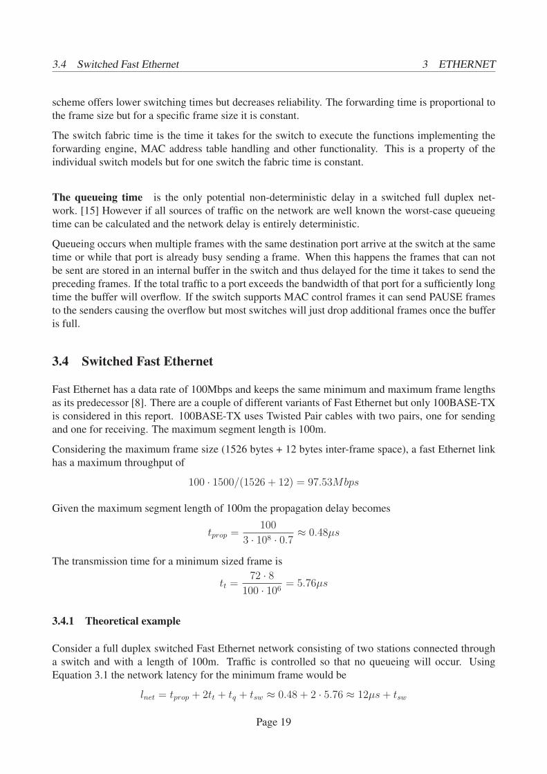
4.1.1 Crossover cable
Figure 4.1: Network topology.
Page 21
4.1 Measured transfer time 4 STUDY OF ETHERNET IN THE SCC2
In this test two control computers were connected using a crossover cable as in Figure 4.1.
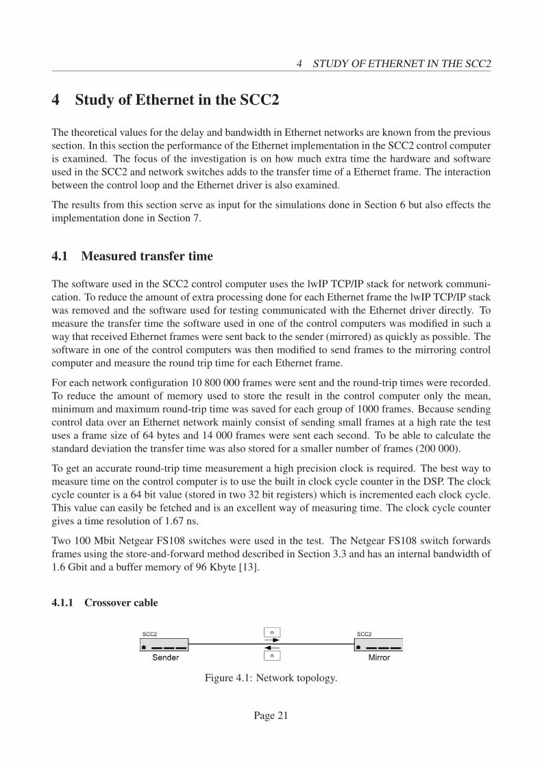
Figure 4.2: Minimum, maximum and mean round-
trip times.
Figure 4.3: Distribution of round-trip times for 200
000 frames.
As can be seen in both Figure 4.2 and Table 4.1 the round-trip time is always in the interval 21.5-26.1
μs with a mean of around 24 μs. This test uses only a crossover cable to connect the two control
computers and this means that every frame is transferred two times across an Ethernet segment. As
given in Section 3.4 the transfer time for an 64 byte Ethernet frame on a 100 Mbit network is 5.76 μs.
Subtracting two times the theoretical transfer time shows that in this test the total hardware and soft-
ware overhead in the control computers is approximately 12.49 μs (for a round-trip transfer). Thus,
the software overhead in one direction is 6.25 μs. Figure 4.3 shows the distribution of round-trip
times.
Total max [μs] Total min [μs] Mean [μs] Standard deviation [μs]
26.07 21.54 24.01 0.1037
Table 4.1: Summary of measurement results
4.1.2 One switch
Figure 4.4: Network topology.
This test uses two control computers connected using a switch as in Figure 4.4.
Page 22
4.1 Measured transfer time 4 STUDY OF ETHERNET IN THE SCC2
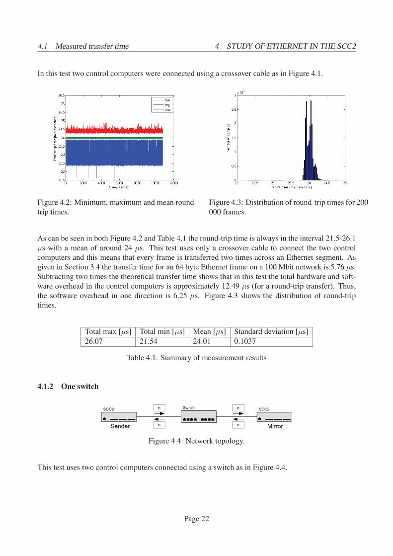
Figure 4.5: Minimum, maximum and mean round-
trip times.
Figure 4.6: Distribution of round-trip times for 200
000 frames.
Adding a switch between the two control computers increases the mean round-trip time with 15.22
μs, from 24.01 μs (Table 4.1) to 39.23 μs (Table 4.2). This increase is because the frame now needs
to be transferred across an additional two Ethernet segments and the switch also needs some time to
forward the frame.
When adding a switch the round-trip times are not centred around the mean as closely as when using
only as crossover cable which can be seen in Figure 4.6.
Total max [μs] Total min [μs] Mean [μs] Standard deviation [μs]
41.75 36.77 39.23 0.2421
Table 4.2: Summary of measurement results
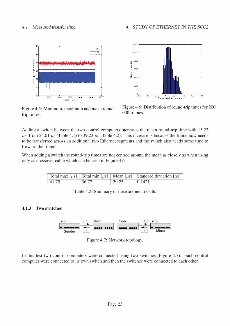
4.1.3 Two switches
Figure 4.7: Network topology.
In this test two control computers were connected using two switches (Figure 4.7). Each control
computer were connected to its own switch and then the switches were connected to each other.
Page 23
4.1 Measured transfer time 4 STUDY OF ETHERNET IN THE SCC2
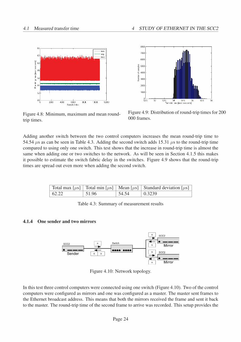
Figure 4.8: Minimum, maximum and mean round-
trip times.
Figure 4.9: Distribution of round-trip times for 200
000 frames.
Adding another switch between the two control computers increases the mean round-trip time to
54.54 μs as can be seen in Table 4.3. Adding the second switch adds 15.31 μs to the round-trip time
compared to using only one switch. This test shows that the increase in round-trip time is almost the
same when adding one or two switches to the network. As will be seen in Section 4.1.5 this makes
it possible to estimate the switch fabric delay in the switches. Figure 4.9 shows that the round-trip
times are spread out even more when adding the second switch.
Total max [μs] Total min [μs] Mean [μs] Standard deviation [μs]
62.22 51.96 54.54 0.3239
Table 4.3: Summary of measurement results
4.1.4 One sender and two mirrors
Figure 4.10: Network topology.
In this test three control computers were connected using one switch (Figure 4.10). Two of the control
computers were configured as mirrors and one was configured as a master. The master sent frames to
the Ethernet broadcast address. This means that both the mirrors received the frame and sent it back
to the master. The round-trip time of the second frame to arrive was recorded. This setup provides the
Page 24
4.1 Measured transfer time 4 STUDY OF ETHERNET IN THE SCC2
opportunity to test how much the round-trip time increases when two control computers send frames
at approximately the same time to the same destination control computer.
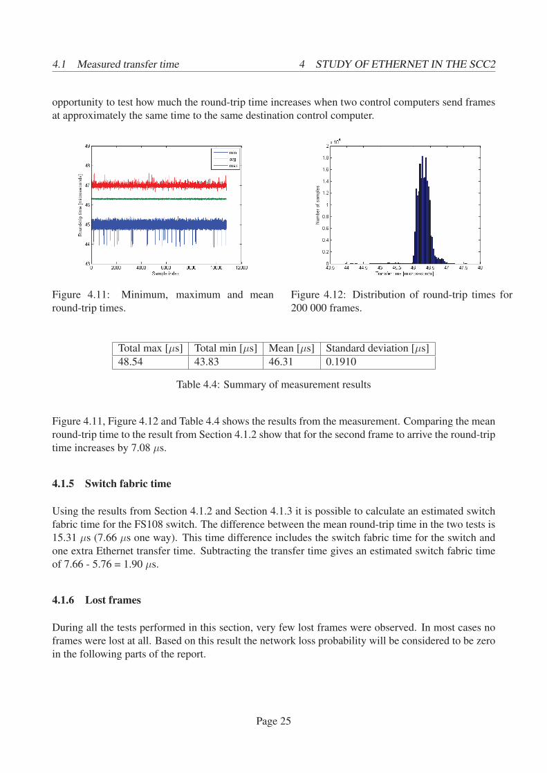
Figure 4.11: Minimum, maximum and mean
round-trip times.
Figure 4.12: Distribution of round-trip times for
200 000 frames.
Total max [μs] Total min [μs] Mean [μs] Standard deviation [μs]
48.54 43.83 46.31 0.1910
Table 4.4: Summary of measurement results
Figure 4.11, Figure 4.12 and Table 4.4 shows the results from the measurement. Comparing the mean
round-trip time to the result from Section 4.1.2 show that for the second frame to arrive the round-trip
time increases by 7.08 μs.
4.1.5 Switch fabric time
Using the results from Section 4.1.2 and Section 4.1.3 it is possible to calculate an estimated switch
fabric time for the FS108 switch. The difference between the mean round-trip time in the two tests is
15.31 μs (7.66 μs one way). This time difference includes the switch fabric time for the switch and
one extra Ethernet transfer time. Subtracting the transfer time gives an estimated switch fabric time
of 7.66 - 5.76 = 1.90 μs.
4.1.6 Lost frames
During all the tests performed in this section, very few lost frames were observed. In most cases no
frames were lost at all. Based on this result the network loss probability will be considered to be zero
in the following parts of the report.
Page 25
4.2 Ethernet driver performance 4 STUDY OF ETHERNET IN THE SCC2
4.2 Ethernet driver performance
The purpose of this test is to measure how much execution time the Ethernet driver uses. This is
important to know because if calls (either reads or writes) to the Ethernet driver is added to control
loop the execution time increases and there are only a limited number of clock cycles available at the
present time.
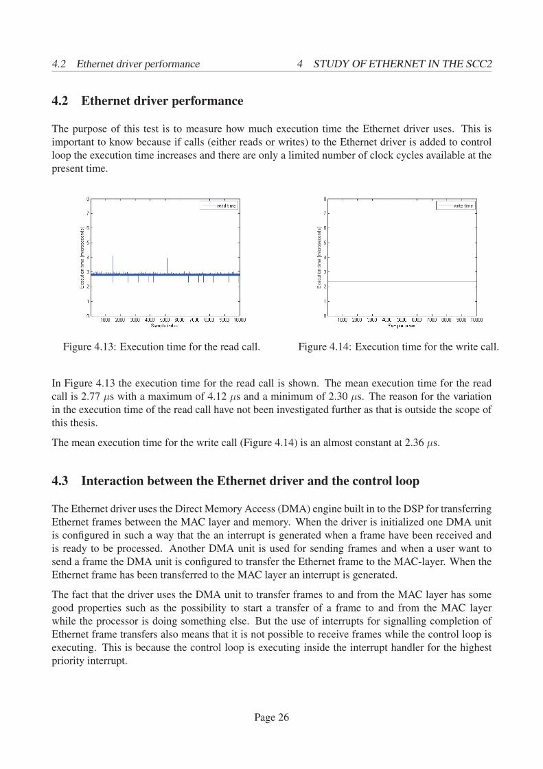
Figure 4.13: Execution time for the read call. Figure 4.14: Execution time for the write call.
In Figure 4.13 the execution time for the read call is shown. The mean execution time for the read
call is 2.77 μs with a maximum of 4.12 μs and a minimum of 2.30 μs. The reason for the variation
in the execution time of the read call have not been investigated further as that is outside the scope of
this thesis.
The mean execution time for the write call (Figure 4.14) is an almost constant at 2.36 μs.
4.3 Interaction between the Ethernet driver and the control loop
The Ethernet driver uses the Direct Memory Access (DMA) engine built in to the DSP for transferring
Ethernet frames between the MAC layer and memory. When the driver is initialized one DMA unit
is configured in such a way that the an interrupt is generated when a frame have been received and
is ready to be processed. Another DMA unit is used for sending frames and when a user want to
send a frame the DMA unit is configured to transfer the Ethernet frame to the MAC-layer. When the
Ethernet frame has been transferred to the MAC layer an interrupt is generated.
The fact that the driver uses the DMA unit to transfer frames to and from the MAC layer has some
good properties such as the possibility to start a transfer of a frame to and from the MAC layer
while the processor is doing something else. But the use of interrupts for signalling completion of
Ethernet frame transfers also means that it is not possible to receive frames while the control loop is
executing. This is because the control loop is executing inside the interrupt handler for the highest
priority interrupt.
Page 26
4.4 Summary 4 STUDY OF ETHERNET IN THE SCC2
4.4 Summary
By measuring frame transfer times between two SCC2 control computers in different network struc-
tures some important results have been found in this section (summarized in Table 4.5). If two SCC2s
are connected via a switch, which is the most likely real-world setup, it takes 19.6 μs from the mo-
ment a data transfer is started until the data is available in the receiving SCC2. This is assuming that
the data size does not exceed 46byte. Out of these 19.6 μs, 6.25 μs consist of delays caused by the
SCC2s (node delay).
Test setup Mean transfer time [μs]
Crossover cable 12.01
One switch 19.62
Two switches 27.27
Table 4.5: Summary of transfer time results
By comparing different setups the delay imposed by the switch could be estimated to approximately
1.90 μs.
The execution times for the send and receive calls are 2.36 μs and 2.77 μs respectively, which is not
insignificant and has to be considered in implementations. Callbacks from the Ethernet driver have
a lower priority than the interrupt which drives the control-loop making also the interaction between
the two an important thing to consider.
Page 27
5 CONTROL ARCHITECTURE IN THE ADF
5 Control architecture in the ADF
In this section the structure and functionality of the existing control algorithm is examined. Special
attention is given to how data flows through the system and how fast different parts needs to be
executed. Requirements for a new system architecture are also identified.
The source code used in this thesis is a specialized version optimized for lab use. The source code
therefore differs from production code in many aspects. The lab code has the advantage of being more
modular and easier to modify than the production code. Despite these difference the results obtained
from the lab code is still applicable on the production code.
The methodology for this investigation includes examining the lab source code for the control algo-
rithms, experiments with a Simulink model of the ADF P300 and interviewing persons responsible
for the control algorithms.
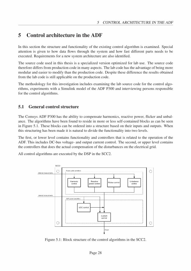
5.1 General control structure
The Comsys ADF P300 has the ability to compensate harmonics, reactive power, flicker and unbal-
ance. The algorithms have been found to reside in more or less self-contained blocks as can be seen
in Figure 5.1. These blocks can be ordered into a structure based on their inputs and outputs. When
this structuring has been made it is natural to divide the functionality into two levels.
The first, or lower level contains functionality and controllers that is related to the operation of the
ADF. This includes DC-bus voltage- and output current control. The second, or upper level contains
the controllers that does the actual compensation of the disturbances on the electrical grid.
All control algorithms are executed by the DSP in the SCC2.
Figure 5.1: Block structure of the control algorithms in the SCC2.
Page 28
5.2 ADF system controllers 5 CONTROL ARCHITECTURE IN THE ADF
5.2 ADF system controllers
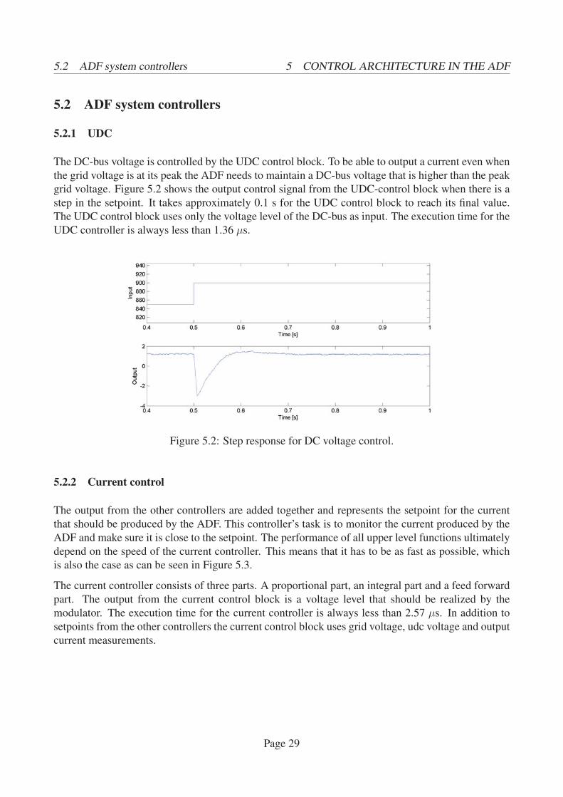
5.2.1 UDC
The DC-bus voltage is controlled by the UDC control block. To be able to output a current even when
the grid voltage is at its peak the ADF needs to maintain a DC-bus voltage that is higher than the peak
grid voltage. Figure 5.2 shows the output control signal from the UDC-control block when there is a
step in the setpoint. It takes approximately 0.1 s for the UDC control block to reach its final value.
The UDC control block uses only the voltage level of the DC-bus as input. The execution time for the
UDC controller is always less than 1.36 μs.
Figure 5.2: Step response for DC voltage control.
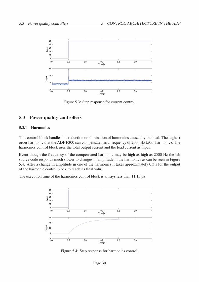
5.2.2 Current control
The output from the other controllers are added together and represents the setpoint for the current
that should be produced by the ADF. This controller’s task is to monitor the current produced by the
ADF and make sure it is close to the setpoint. The performance of all upper level functions ultimately
depend on the speed of the current controller. This means that it has to be as fast as possible, which
is also the case as can be seen in Figure 5.3.
The current controller consists of three parts. A proportional part, an integral part and a feed forward
part. The output from the current control block is a voltage level that should be realized by the
modulator. The execution time for the current controller is always less than 2.57 μs. In addition to
setpoints from the other controllers the current control block uses grid voltage, udc voltage and output
current measurements.
Page 29
5.3 Power quality controllers 5 CONTROL ARCHITECTURE IN THE ADF
Figure 5.3: Step response for current control.
5.3 Power quality controllers
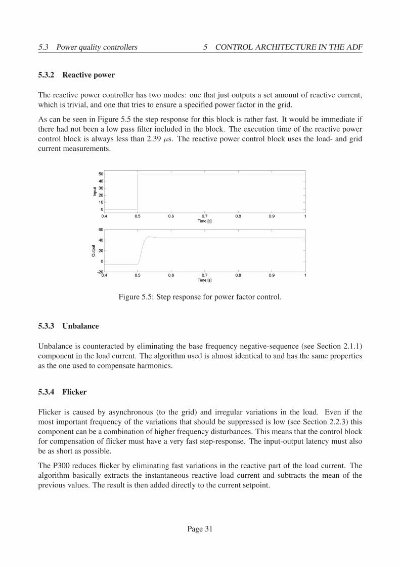
5.3.1 Harmonics
This control block handles the reduction or elimination of harmonics caused by the load. The highest
order harmonic that the ADF P300 can compensate has a frequency of 2500 Hz (50th harmonic). The
harmonics control block uses the total output current and the load current as input.
Event though the frequency of the compensated harmonic may be high as high as 2500 Hz the lab
source code responds much slower to changes in amplitude in the harmonics as can be seen in Figure
5.4. After a change in amplitude in one of the harmonics it takes approximately 0.3 s for the output
of the harmonic control block to reach its final value.
The execution time of the harmonics control block is always less than 11.15 μs.
Figure 5.4: Step response for harmonics control.
Page 30
5.3 Power quality controllers 5 CONTROL ARCHITECTURE IN THE ADF
5.3.2 Reactive power
The reactive power controller has two modes: one that just outputs a set amount of reactive current,
which is trivial, and one that tries to ensure a specified power factor in the grid.
As can be seen in Figure 5.5 the step response for this block is rather fast. It would be immediate if
there had not been a low pass filter included in the block. The execution time of the reactive power
control block is always less than 2.39 μs. The reactive power control block uses the load- and grid
current measurements.
Figure 5.5: Step response for power factor control.
5.3.3 Unbalance
Unbalance is counteracted by eliminating the base frequency negative-sequence (see Section 2.1.1)
component in the load current. The algorithm used is almost identical to and has the same properties
as the one used to compensate harmonics.
5.3.4 Flicker
Flicker is caused by asynchronous (to the grid) and irregular variations in the load. Even if the
most important frequency of the variations that should be suppressed is low (see Section 2.2.3) this
component can be a combination of higher frequency disturbances. This means that the control block
for compensation of flicker must have a very fast step-response. The input-output latency must also
be as short as possible.
The P300 reduces flicker by eliminating fast variations in the reactive part of the load current. The
algorithm basically extracts the instantaneous reactive load current and subtracts the mean of the
previous values. The result is then added directly to the current setpoint.
Page 31

5.4 Identified requirements 5 CONTROL ARCHITECTURE IN THE ADF
It is hard to simulate a load that causes flicker and the Simulink model used in these simulations
contains no such load which is why no step response was made for the flicker block. The execution
time of the flicker control block is always less than 1.78μs.
5.4 Identified requirements
A distributed control architecture should mainly be evaluated based on two characteristics: robustness
and performance. The robustness criteria includes being able to handle communication problems like
lost packets and corrupted data.
Performance wise the distributed system should have minimal additional execution time compared to
the original system. The highest harmonic possible to compensate should not be affected negatively.
Changes in response time and the effects on general control performance should be closely monitored.
5.5 Test case
To be able to evaluate the distributed control architecture and compare it to the original system a test
case and a number of variables to monitor have been identified. The test case consist of five different
changes in the load rather than changes to the input to the individual control blocks. This choice was
made because it simulates real world situations. If the load changes are designed correctly they can
provide worst-case scenarios without generating unrealistic signals. This approach also ensures that
all components of the system and their interactions are tested. Details about the test load will be given
in Section 6.3.1.
To make sure that the ADF operates within its specified limits a number of signals and internal states
should be monitored. The following signals and states of importance have been identified:
• DC-bus voltage
• The output from the different controllers
• The grid current
5.6 Summary
The controllers of the ADF P300 lab code can be structured in a block diagram and divided into two
groups: controllers for the hardware and controllers for power quality parameters.
The speed of the step response vary between the blocks from almost instant responses to as much as
0.3 s which is long compared to both the grid frequency and the sampling frequency of the system.
Comparing even the fastest power quality controller (the reactive power controller) with the network
transfer time measured in Section 4 it can be seen that the controllers response time is a factor 1000
larger than the network transfer time.
Page 32
5.6 Summary 5 CONTROL ARCHITECTURE IN THE ADF
The harmonics control block has by far the longest execution time of approximately 11μs while the
other blocks take approximately 2μs to execute.
A number of requirements for the distributed system has been identified. These can be organized into
two groups, robustness requirements and performance requirements. To verify these requirements a
test strategy has been developed which implies that the whole system is tested through load changes.
Page 33
6 A DISTRIBUTED CONTROL ARCHITECTURE
6 A distributed control architecture
In this section a distributed control architecture is designed based on results and observations from
the previous sections. This design is then tested through simulations using different test loads. The
tools used for the simulations are briefly introduced together with a Simulink model of the ADF.
6.1 Design
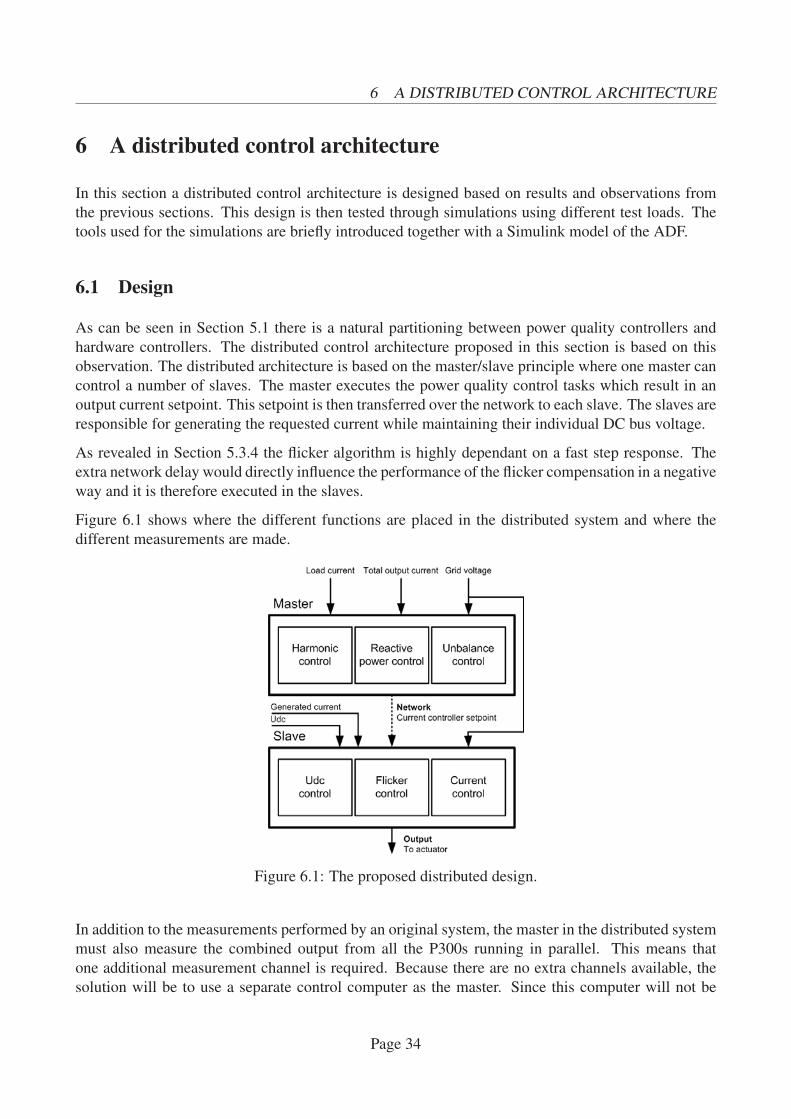
As can be seen in Section 5.1 there is a natural partitioning between power quality controllers and
hardware controllers. The distributed control architecture proposed in this section is based on this
observation. The distributed architecture is based on the master/slave principle where one master can
control a number of slaves. The master executes the power quality control tasks which result in an
output current setpoint. This setpoint is then transferred over the network to each slave. The slaves are
responsible for generating the requested current while maintaining their individual DC bus voltage.
As revealed in Section 5.3.4 the flicker algorithm is highly dependant on a fast step response. The
extra network delay would directly influence the performance of the flicker compensation in a negative
way and it is therefore executed in the slaves.
Figure 6.1 shows where the different functions are placed in the distributed system and where the
different measurements are made.
Figure 6.1: The proposed distributed design.
In addition to the measurements performed by an original system, the master in the distributed system
must also measure the combined output from all the P300s running in parallel. This means that
one additional measurement channel is required. Because there are no extra channels available, the
solution will be to use a separate control computer as the master. Since this computer will not be
Page 34
6.2 Simulation tools 6 A DISTRIBUTED CONTROL ARCHITECTURE
connected to any PPs the channel otherwise used to measure the output current can be used for the
combined output current instead.
6.1.1 Motivation
The main objective of an ADF is to eliminate or reduce power quality problems. Even if multiple
systems are used in parallel there is still just one power quality situation that has to be resolved and it
is thus unnecessary that all systems execute the power quality controllers themselves. In the proposed
design power quality control is done in only one place, the master, and the result is then distributed
to the slaves. This can be seen as an added abstraction layer where the master just has to decide the
output current and no longer needs to know the details of generating it.
One of the most important things to consider when designing this distributed control system is safety.
In this context safety means that the system should behave in a controlled manner and not damage
itself, other equipment, or in the worst case injure human beings. If data is lost or corrupted the
system should degrade gracefully. In the chosen design the hardware controllers are not dependent
on the Ethernet network at all. This means that the system is inherently safe against network failures
since the control of the hardware such as the DC bus is not affected.
As can be seen in Section 5.3.1 the step responses of the harmonics, unbalance and cos ϕ controllers
are slow with respect to the sampling frequency. The additional delay imposed by the network (see
Section 4) is very small in comparison to these controllers settling time. Thus the performance of
these functions should not be significantly affected by the added network delay.
One possible problem with the design is that the system is highly dependent on the master control
computer. A hardware or software failure in the master control computer will render all the ADFs
unusable until the problem with the master control computer can be solved.
6.2 Simulation tools
6.2.1 Simulink model
A model was developed in MATLAB/Simulink for the purpose of simulating the ADF. This model
simulates a electrical three-phase grid, a load and an ADF. The load can be configured to generate
reactive currents, harmonics and unbalance. It can be connected or disconnected at any time using a
breaker, which enables analysis of how the whole system reacts to steps in the load. The ADF model
is implemented as a triggered subsystem with ts = 1/14400 s.
Most of the model is implemented graphically with standard blocks except for the harmonic, Udc and
current control algorithms. These are implemented as MATLab functions which are ported from the
C code of the P300.
Page 35

6.2 Simulation tools 6 A DISTRIBUTED CONTROL ARCHITECTURE
6.2.2 Using TrueTime to simulate network transfer
TrueTime is developed by the Department of Automatic Control at Lund University. It is a MAT-
Lab/Simulink framework whose main objective is to provide the tools needed for simulation of em-
bedded real-time control systems. TrueTime also contains blocks that simulate network transfers on
a variety of different networks, including Switched Ethernet [5].
Figure 6.2: The TrueTime Simulink blocks.
Figure 6.2 shows the blocks provided by the TrueTime library. Only the network blocks (TrueTime
Network, TrueTime Send and TrueTime Receive) are used in this thesis.
The TrueTime network blocks only model delays imposed by the actual network and not by the
software and hardware in the nodes. There is a possibility to add node delays in TrueTime, but then a
TrueTime Kernel block must be used.
Figure 6.3: Model showing the blocks used to simulate network delay in a simplified context.
Page 36
6.3 Experimental setup 6 A DISTRIBUTED CONTROL ARCHITECTURE
Instead a Variable Time Delay Simulink block is used to simulate the node delays. This block was
fed with delay data recorded in Section 4.1.1. The model used to simulate the network is shown in
Figure 6.3.
The following significant settings were used for the TrueTime Network blocks:
TrueTime NetworkNetwork Type Switched Ethernet
Data rate 100000000 bits/s
Min frame size 512 bits
Loss probability 0
Switch memory 80000 bits
Switch overflow behaviour Drop
TrueTime SendData Length 512 bits
6.3 Experimental setup
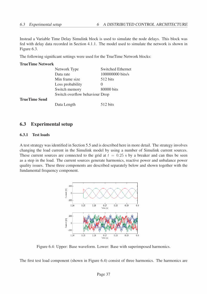
6.3.1 Test loads
A test strategy was identified in Section 5.5 and is described here in more detail. The strategy involves
changing the load current in the Simulink model by using a number of Simulink current sources.
These current sources are connected to the grid at t = 0.25 s by a breaker and can thus be seen
as a step in the load. The current sources generate harmonics, reactive power and unbalance power
quality issues. These three components are described separately below and shown together with the
fundamental frequency component.
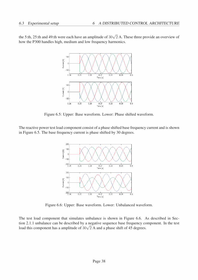
Figure 6.4: Upper: Base waveform. Lower: Base with superimposed harmonics.
The first test load component (shown in Figure 6.4) consist of three harmonics. The harmonics are
Page 37
6.3 Experimental setup 6 A DISTRIBUTED CONTROL ARCHITECTURE
the 5:th, 25:th and 49:th were each have an amplitude of 30√2 A. These three provide an overview of
how the P300 handles high, medium and low frequency harmonics.
Figure 6.5: Upper: Base waveform. Lower: Phase shifted waveform.
The reactive power test load component consist of a phase shifted base frequency current and is shown
in Figure 6.5. The base frequency current is phase shifted by 30 degrees.
Figure 6.6: Upper: Base waveform. Lower: Unbalanced waveform.
The test load component that simulates unbalance is shown in Figure 6.6. As described in Sec-
tion 2.1.1 unbalance can be described by a negative sequence base frequency component. In the test
load this component has a amplitude of 30√2 A and a phase shift of 45 degrees.
Page 38
6.3 Experimental setup 6 A DISTRIBUTED CONTROL ARCHITECTURE
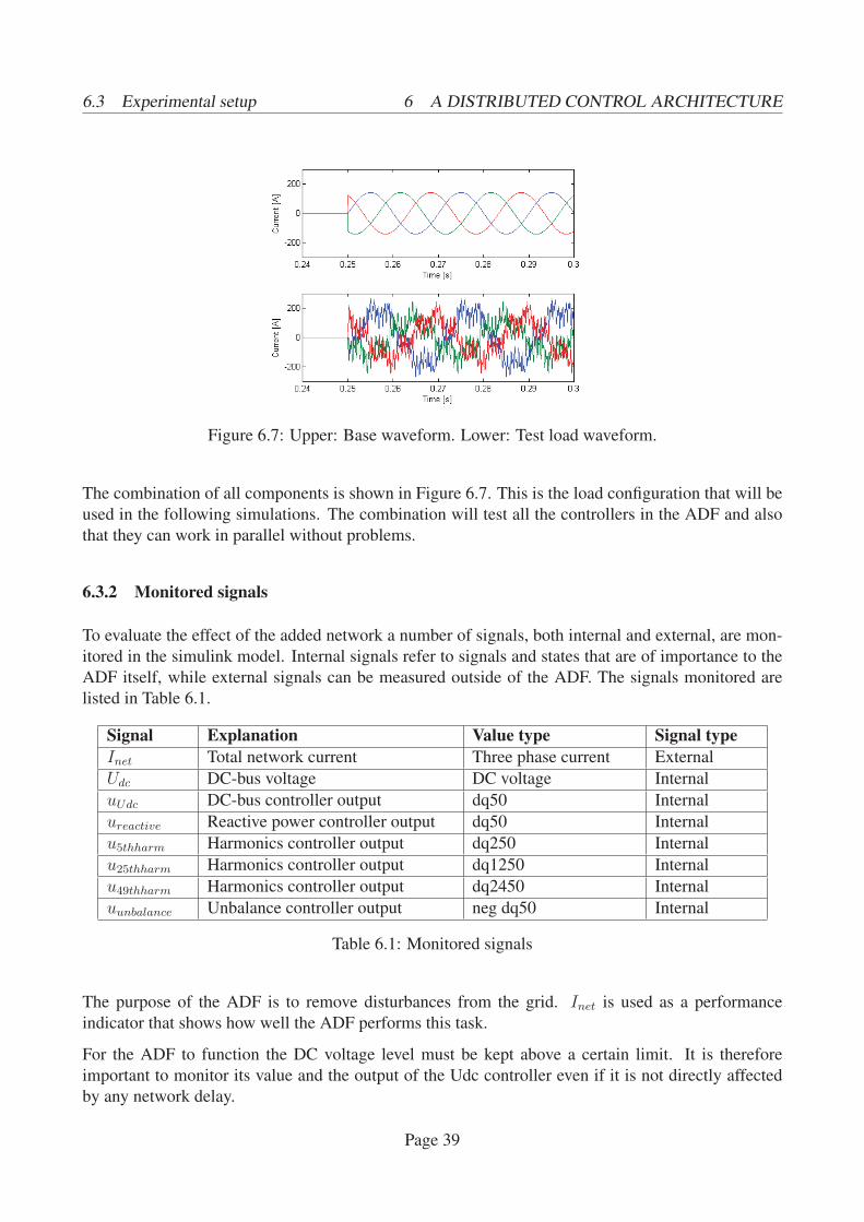
Figure 6.7: Upper: Base waveform. Lower: Test load waveform.
The combination of all components is shown in Figure 6.7. This is the load configuration that will be
used in the following simulations. The combination will test all the controllers in the ADF and also
that they can work in parallel without problems.
6.3.2 Monitored signals
To evaluate the effect of the added network a number of signals, both internal and external, are mon-
itored in the simulink model. Internal signals refer to signals and states that are of importance to the
ADF itself, while external signals can be measured outside of the ADF. The signals monitored are
listed in Table 6.1.
Signal Explanation Value type Signal typeInet Total network current Three phase current External
Udc DC-bus voltage DC voltage Internal
uUdc DC-bus controller output dq50 Internal
ureactive Reactive power controller output dq50 Internal
u5thharm Harmonics controller output dq250 Internal
u25thharm Harmonics controller output dq1250 Internal
u49thharm Harmonics controller output dq2450 Internal
uunbalance Unbalance controller output neg dq50 Internal
Table 6.1: Monitored signals
The purpose of the ADF is to remove disturbances from the grid. Inet is used as a performance
indicator that shows how well the ADF performs this task.
For the ADF to function the DC voltage level must be kept above a certain limit. It is therefore
important to monitor its value and the output of the Udc controller even if it is not directly affected
by any network delay.
Page 39
6.4 A first attempt 6 A DISTRIBUTED CONTROL ARCHITECTURE
Most of the internal signals are represented in rotating dq coordinates according to Section 2.1.3.
To get rid of oscillations that would obscure the behaviours of interest the output of the harmonic
controllers are monitored separately in their corresponding reference frame.
The power quality controller outputs, ux, are monitored to see how the individual controllers are
working. Since they have different characteristics the network delay will impact their performance
differently.
6.3.3 Sampling
The sampling in the original system is synchronized with the switching of the IGBT in such a way
that sampling will always be done in between two commutations. This approach ensures that the
ripple, which is a by-product of switching, affects the sampling as little as possible. This will be a
problem with multiple systems since the switch ripple from one system will affect the sampling of
other systems.
The problems associated with sampling is outside the scope of this thesis and will therefore not be
considered further. These problems are also easily avoided in the simulations where the master and
slaves can use synchronized clocks.
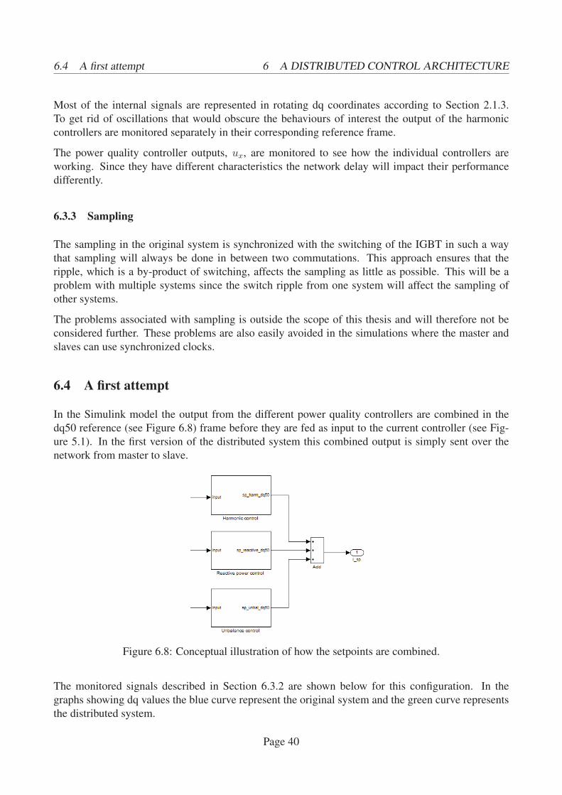
6.4 A first attempt
In the Simulink model the output from the different power quality controllers are combined in the
dq50 reference (see Figure 6.8) frame before they are fed as input to the current controller (see Fig-
ure 5.1). In the first version of the distributed system this combined output is simply sent over the
network from master to slave.
Figure 6.8: Conceptual illustration of how the setpoints are combined.
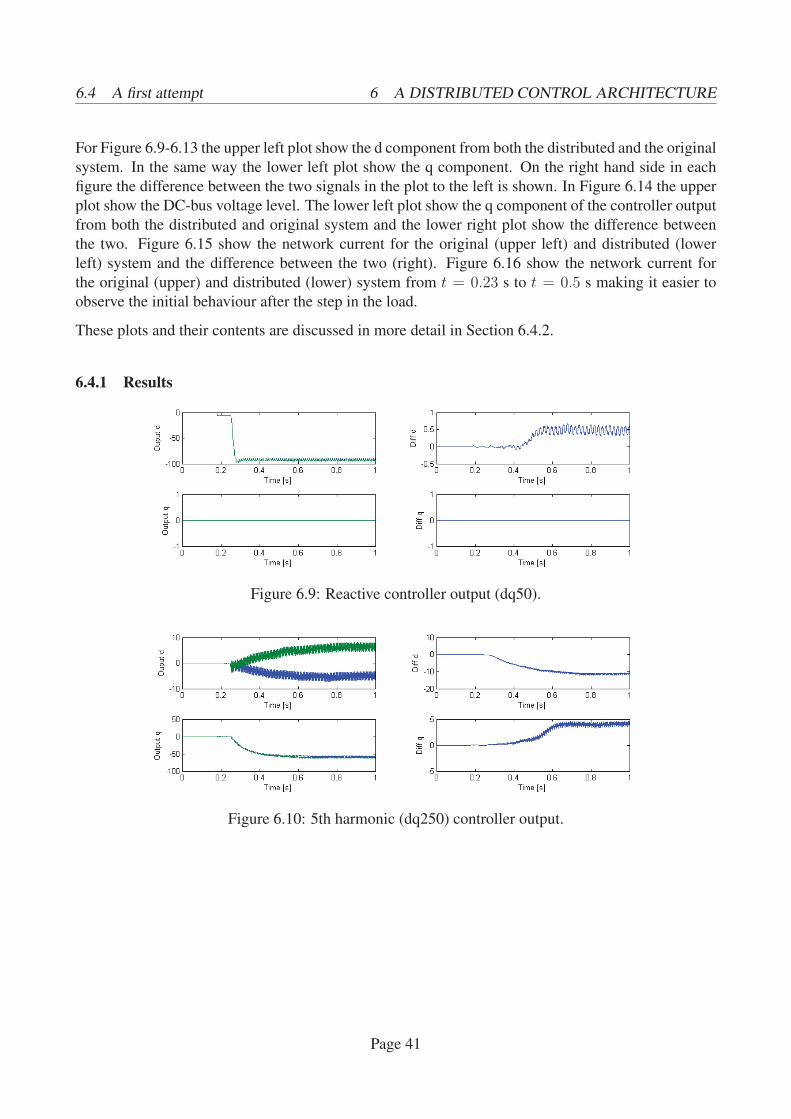
The monitored signals described in Section 6.3.2 are shown below for this configuration. In the
graphs showing dq values the blue curve represent the original system and the green curve represents
the distributed system.
Page 40
6.4 A first attempt 6 A DISTRIBUTED CONTROL ARCHITECTURE
For Figure 6.9-6.13 the upper left plot show the d component from both the distributed and the original
system. In the same way the lower left plot show the q component. On the right hand side in each
figure the difference between the two signals in the plot to the left is shown. In Figure 6.14 the upper
plot show the DC-bus voltage level. The lower left plot show the q component of the controller output
from both the distributed and original system and the lower right plot show the difference between
the two. Figure 6.15 show the network current for the original (upper left) and distributed (lower
left) system and the difference between the two (right). Figure 6.16 show the network current for
the original (upper) and distributed (lower) system from t = 0.23 s to t = 0.5 s making it easier to
observe the initial behaviour after the step in the load.
These plots and their contents are discussed in more detail in Section 6.4.2.
6.4.1 Results
Figure 6.9: Reactive controller output (dq50).
Figure 6.10: 5th harmonic (dq250) controller output.
Page 41

6.4 A first attempt 6 A DISTRIBUTED CONTROL ARCHITECTURE
Figure 6.11: 25th harmonic (dq1250) controller output.
Figure 6.12: 49th harmonic (dq2450) controller output.
Figure 6.13: Unbalance controller output (neg dq50).
Figure 6.14: DC-bus value and controller output.
Page 42
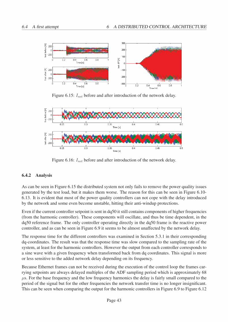
6.4 A first attempt 6 A DISTRIBUTED CONTROL ARCHITECTURE
Figure 6.15: Inet before and after introduction of the network delay.
Figure 6.16: Inet before and after introduction of the network delay.
6.4.2 Analysis
As can be seen in Figure 6.15 the distributed system not only fails to remove the power quality issues
generated by the test load, but it makes them worse. The reason for this can be seen in Figure 6.10-
6.13. It is evident that most of the power quality controllers can not cope with the delay introduced
by the network and some even become unstable, hitting their anti-windup protections.
Even if the current controller setpoint is sent in dq50 it still contains components of higher frequencies
(from the harmonic controller). These components will oscillate, and thus be time dependent, in the
dq50 reference frame. The only controller operating directly in the dq50 frame is the reactive power
controller, and as can be seen in Figure 6.9 it seems to be almost unaffected by the network delay.
The response time for the different controllers was examined in Section 5.3.1 in their corresponding
dq-coordinates. The result was that the response time was slow compared to the sampling rate of the
system, at least for the harmonic controllers. However the output from each controller corresponds to
a sine wave with a given frequency when transformed back from dq coordinates. This signal is more
or less sensitive to the added network delay depending on its frequency.
Because Ethernet frames can not be received during the execution of the control loop the frames car-
rying setpoints are always delayed multiples of the ADF sampling period which is approximately 68
μs. For the base frequency and the low frequency harmonics the delay is fairly small compared to the
period of the signal but for the other frequencies the network transfer time is no longer insignificant.
This can be seen when comparing the output for the harmonic controllers in Figure 6.9 to Figure 6.12
Page 43

6.5 A better approach 6 A DISTRIBUTED CONTROL ARCHITECTURE
where the controllers handling high frequency harmonics are more severely affected by the added
delay than the ones handling lower frequencies.
All digital control systems (such as the P300) have a certain input-output delay. In the lab implemen-
tation of the ADF a compensation is done for this delay. The compensation is increasingly important
for the higher frequency harmonics [7].
The compensation for the input-output delay should include the added network delay.
6.5 A better approach
In this section an approach is tested where the network transfer delay is included in the input-output
delay compensation.
Because the setpoint from the power quality controllers always generate some type of sinusoidal
waveform it is possible to compensate for the input-output delay. The general idea behind the com-
pensation is to use
A sinωxt2 = A sin(ωx(t1 + tdelay)) = A sin(ωxt1 + ϕx) (6.1)
where t1 is the sampling time and t2 is the time when the setpoint is expected to be used. For each
signal that require compensation the compensation angle (ϕx) must be calculated and this angle de-
pends on the frequency of the signal. If the input-output delay of the system is constant then ϕx is
also constant for a given frequency. In the P300 the output signals from the controllers are vectors in
the dq-plane and the compensation is done by rotating the vector after it has been transformed back
to the αβ-plane as shown in Equation 6.2.
[Xα
Xβ
]=
[cosϕx sinϕx
− sinϕx cosϕx
] [cosωxt1 − sinωxt1sinωxt1 cosωxt1
] [Xd
Xq
](6.2)
A straight forward approach for including the network delay in the compensation would be to calcu-
late a new ϕx by including the network delay in tdelay. The compensation must be done separately for
each signal before the signals are added together in the dq50 reference frame. This also means that in
the distributed system the compensation must be done on the master before the setpoint is transferred
across the network. Unfortunately the network transfer delay varies as seen in Section 4. Therefore
the exact transfer time is not known before the setpoint have actually been transferred. It is therefore
only possible to compensate for the average transfer time on the master.
Page 44
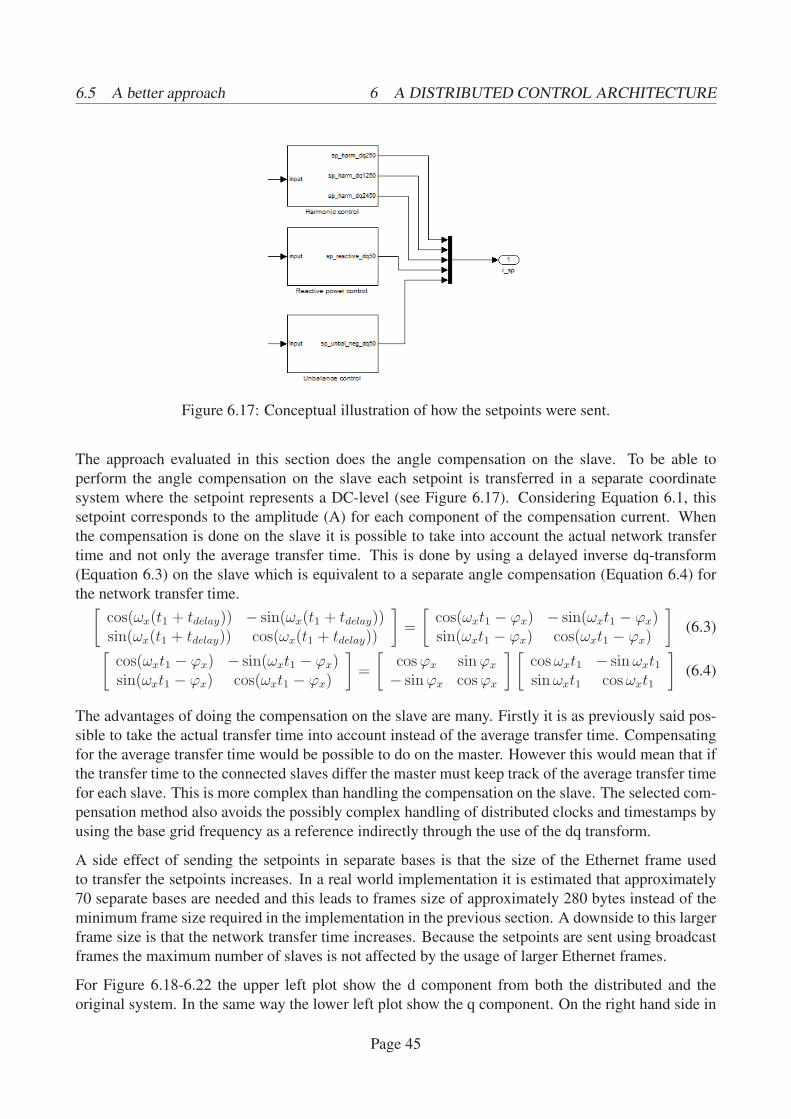
6.5 A better approach 6 A DISTRIBUTED CONTROL ARCHITECTURE
Figure 6.17: Conceptual illustration of how the setpoints were sent.
The approach evaluated in this section does the angle compensation on the slave. To be able to
perform the angle compensation on the slave each setpoint is transferred in a separate coordinate
system where the setpoint represents a DC-level (see Figure 6.17). Considering Equation 6.1, this
setpoint corresponds to the amplitude (A) for each component of the compensation current. When
the compensation is done on the slave it is possible to take into account the actual network transfer
time and not only the average transfer time. This is done by using a delayed inverse dq-transform
(Equation 6.3) on the slave which is equivalent to a separate angle compensation (Equation 6.4) for
the network transfer time.[cos(ωx(t1 + tdelay)) − sin(ωx(t1 + tdelay))sin(ωx(t1 + tdelay)) cos(ωx(t1 + tdelay))
]=
[cos(ωxt1 − ϕx) − sin(ωxt1 − ϕx)sin(ωxt1 − ϕx) cos(ωxt1 − ϕx)
](6.3)
[cos(ωxt1 − ϕx) − sin(ωxt1 − ϕx)sin(ωxt1 − ϕx) cos(ωxt1 − ϕx)
]=
[cosϕx sinϕx
− sinϕx cosϕx
] [cosωxt1 − sinωxt1sinωxt1 cosωxt1
](6.4)
The advantages of doing the compensation on the slave are many. Firstly it is as previously said pos-
sible to take the actual transfer time into account instead of the average transfer time. Compensating
for the average transfer time would be possible to do on the master. However this would mean that if
the transfer time to the connected slaves differ the master must keep track of the average transfer time
for each slave. This is more complex than handling the compensation on the slave. The selected com-
pensation method also avoids the possibly complex handling of distributed clocks and timestamps by
using the base grid frequency as a reference indirectly through the use of the dq transform.
A side effect of sending the setpoints in separate bases is that the size of the Ethernet frame used
to transfer the setpoints increases. In a real world implementation it is estimated that approximately
70 separate bases are needed and this leads to frames size of approximately 280 bytes instead of the
minimum frame size required in the implementation in the previous section. A downside to this larger
frame size is that the network transfer time increases. Because the setpoints are sent using broadcast
frames the maximum number of slaves is not affected by the usage of larger Ethernet frames.
For Figure 6.18-6.22 the upper left plot show the d component from both the distributed and the
original system. In the same way the lower left plot show the q component. On the right hand side in
Page 45
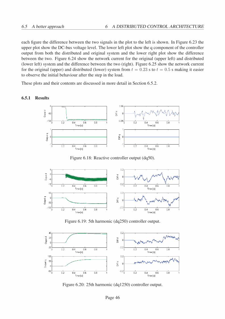
6.5 A better approach 6 A DISTRIBUTED CONTROL ARCHITECTURE
each figure the difference between the two signals in the plot to the left is shown. In Figure 6.23 the
upper plot show the DC-bus voltage level. The lower left plot show the q component of the controller
output from both the distributed and original system and the lower right plot show the difference
between the two. Figure 6.24 show the network current for the original (upper left) and distributed
(lower left) system and the difference between the two (right). Figure 6.25 show the network current
for the original (upper) and distributed (lower) system from t = 0.23 s to t = 0.5 s making it easier
to observe the initial behaviour after the step in the load.
These plots and their contents are discussed in more detail in Section 6.5.2.
6.5.1 Results
Figure 6.18: Reactive controller output (dq50).
Figure 6.19: 5th harmonic (dq250) controller output.
Figure 6.20: 25th harmonic (dq1250) controller output.
Page 46
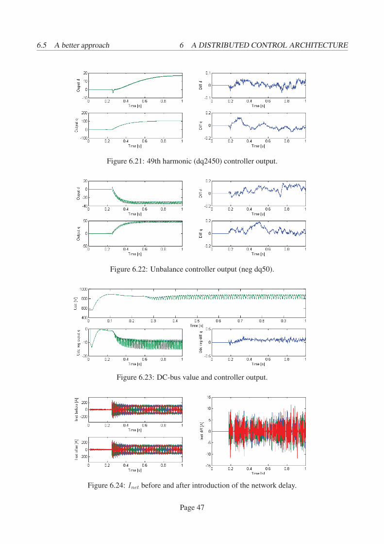
6.5 A better approach 6 A DISTRIBUTED CONTROL ARCHITECTURE
Figure 6.21: 49th harmonic (dq2450) controller output.
Figure 6.22: Unbalance controller output (neg dq50).
Figure 6.23: DC-bus value and controller output.
Figure 6.24: Inet before and after introduction of the network delay.
Page 47
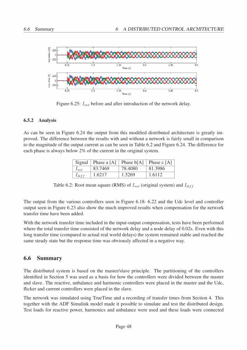
6.6 Summary 6 A DISTRIBUTED CONTROL ARCHITECTURE
Figure 6.25: Inet before and after introduction of the network delay.
6.5.2 Analysis
As can be seen in Figure 6.24 the output from this modified distributed architecture is greatly im-
proved. The difference between the results with and without a network is fairly small in comparison
to the magnitude of the output current as can be seen in Table 6.2 and Figure 6.24. The difference for
each phase is always below 2% of the current in the original system.
Signal Phase a [A] Phase b[A] Phase c [A]
Inet 83.7469 78.4080 81.3986
Idiff 1.6217 1.5269 1.6112
Table 6.2: Root mean square (RMS) of Inet (original system) and Idiff
The output from the various controllers seen in Figure 6.18- 6.22 and the Udc level and controller
output seen in Figure 6.23 also show the much improved results when compensation for the network
transfer time have been added.
With the network transfer time included in the input-output compensation, tests have been performed
where the total transfer time consisted of the network delay and a node delay of 0.02s. Even with this
long transfer time (compared to actual real world delays) the system remained stable and reached the
same steady state but the response time was obviously affected in a negative way.
6.6 Summary
The distributed system is based on the master/slave principle. The partitioning of the controllers
identified in Section 5 was used as a basis for how the controllers were divided between the master
and slave. The reactive, unbalance and harmonic controllers were placed in the master and the Udc,
flicker and current controllers were placed in the slave.
The network was simulated using TrueTime and a recording of transfer times from Section 4. This
together with the ADF Simulink model made it possible to simulate and test the distributed design.
Test loads for reactive power, harmonics and unbalance were used and these loads were connected
Page 48
6.6 Summary 6 A DISTRIBUTED CONTROL ARCHITECTURE
using a breaker. This together with the monitoring of a set of signals made it possible to see how the
different controllers reacted to a step in the load.
The first attempt did not work at all because no compensation was done for the added network delay.
When this delay was compensated for the system worked very well and there was only small differ-
ences compared to the original system. The distributed system was also tested with delays up to 0.02
s and remained stable, though with severely degraded response times.
Page 49
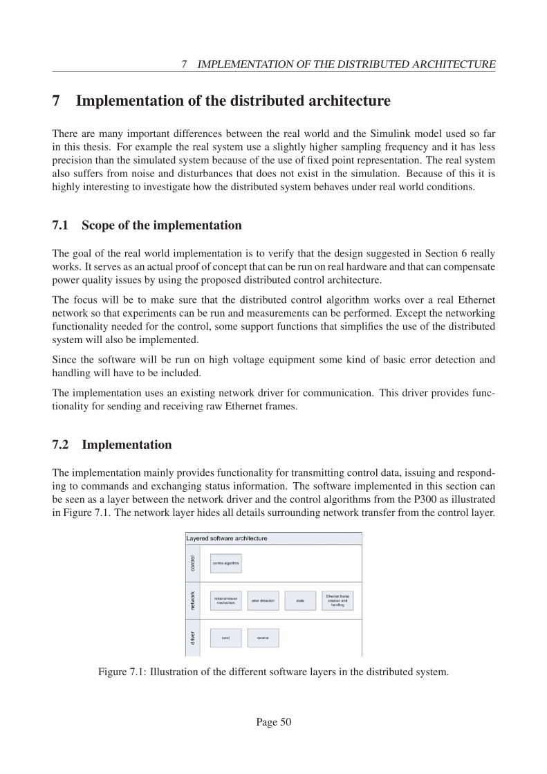
7 IMPLEMENTATION OF THE DISTRIBUTED ARCHITECTURE
7 Implementation of the distributed architecture
There are many important differences between the real world and the Simulink model used so far
in this thesis. For example the real system use a slightly higher sampling frequency and it has less
precision than the simulated system because of the use of fixed point representation. The real system
also suffers from noise and disturbances that does not exist in the simulation. Because of this it is
highly interesting to investigate how the distributed system behaves under real world conditions.
7.1 Scope of the implementation
The goal of the real world implementation is to verify that the design suggested in Section 6 really
works. It serves as an actual proof of concept that can be run on real hardware and that can compensate
power quality issues by using the proposed distributed control architecture.
The focus will be to make sure that the distributed control algorithm works over a real Ethernet
network so that experiments can be run and measurements can be performed. Except the networking
functionality needed for the control, some support functions that simplifies the use of the distributed
system will also be implemented.
Since the software will be run on high voltage equipment some kind of basic error detection and
handling will have to be included.
The implementation uses an existing network driver for communication. This driver provides func-
tionality for sending and receiving raw Ethernet frames.
7.2 Implementation
The implementation mainly provides functionality for transmitting control data, issuing and respond-
ing to commands and exchanging status information. The software implemented in this section can
be seen as a layer between the network driver and the control algorithms from the P300 as illustrated
in Figure 7.1. The network layer hides all details surrounding network transfer from the control layer.
Figure 7.1: Illustration of the different software layers in the distributed system.
Page 50
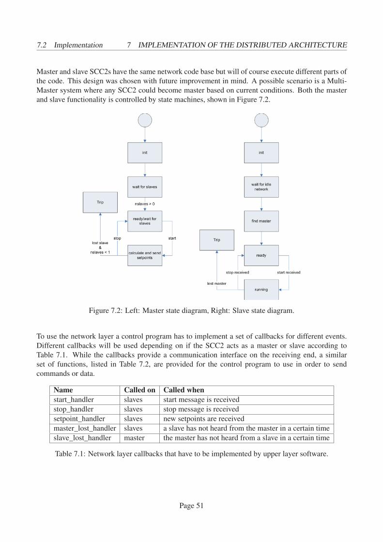
7.2 Implementation 7 IMPLEMENTATION OF THE DISTRIBUTED ARCHITECTURE
Master and slave SCC2s have the same network code base but will of course execute different parts of
the code. This design was chosen with future improvement in mind. A possible scenario is a Multi-
Master system where any SCC2 could become master based on current conditions. Both the master
and slave functionality is controlled by state machines, shown in Figure 7.2.
Figure 7.2: Left: Master state diagram, Right: Slave state diagram.
To use the network layer a control program has to implement a set of callbacks for different events.
Different callbacks will be used depending on if the SCC2 acts as a master or slave according to
Table 7.1. While the callbacks provide a communication interface on the receiving end, a similar
set of functions, listed in Table 7.2, are provided for the control program to use in order to send
commands or data.
Name Called on Called whenstart_handler slaves start message is received
stop_handler slaves stop message is received
setpoint_handler slaves new setpoints are received
master_lost_handler slaves a slave has not heard from the master in a certain time
slave_lost_handler master the master has not heard from a slave in a certain time
Table 7.1: Network layer callbacks that have to be implemented by upper layer software.
Page 51

7.2 Implementation 7 IMPLEMENTATION OF THE DISTRIBUTED ARCHITECTURE
Name Used by Purposenetwork master and slaves drives the network functionality
issue_start master Tell connected slaves to start
issue_stop master Tell connected slaves to stop
send_setpoints master Send new setpoints to slaves
send_heartbeat slaves Tell the master that the slave is ok
Table 7.2: Network layer functions that can be used by upper layer software.
The network function should be called periodically, preferably from the control loop, since it is this
function that actually call the network driver to send frames. This design is motivated in Section 7.2.1.
The network function also handles retransmission and error detection as described in Section 7.2.3
and Section 7.2.4.
7.2.1 Concurrency issues
There are three contexts in which data or events that have to be sent over the network are generated:
the control loop (setpoints), the network driver received frame callback (acknowledgements) and the
thread that handles user interaction (start,stop). Many problems arise if these contexts could call the
network send function asynchronously:
• Certain messages have higher priority (see Table 7.3) and could potentially be delayed by lower
priority messages already in progress.
• The network driver would need to be supplied with more than one buffer to allow multiple
messages to be queued (in the driver).
• The maximum execution time would increase since multiple events causing network transfer
could stack up.
Thus, allowing asynchronous access to the network would have a negative impact on memory usage,
worst case execution time and responsiveness to important events such as the Stop event.
A simple approach to address these problems is to only call the send function from one place. Then
the execution time for the network functionality is limited by only sending one message per cycle. As
described in Section 4.3 the control loop is executed in the context of the highest priority interrupt. If
frames are sent from this context it is not possible for any other process to interfere and therefore the
software delay should be minimal.
If network data is generated elsewhere it is prepared to be sent but then stored in an array of frame
structures together with a flag that indicates if there is data pending for that particular type. When the
control loop executes the network function it will look in the frame array for pending frames and send
one frame each iteration according to priority.
Page 52
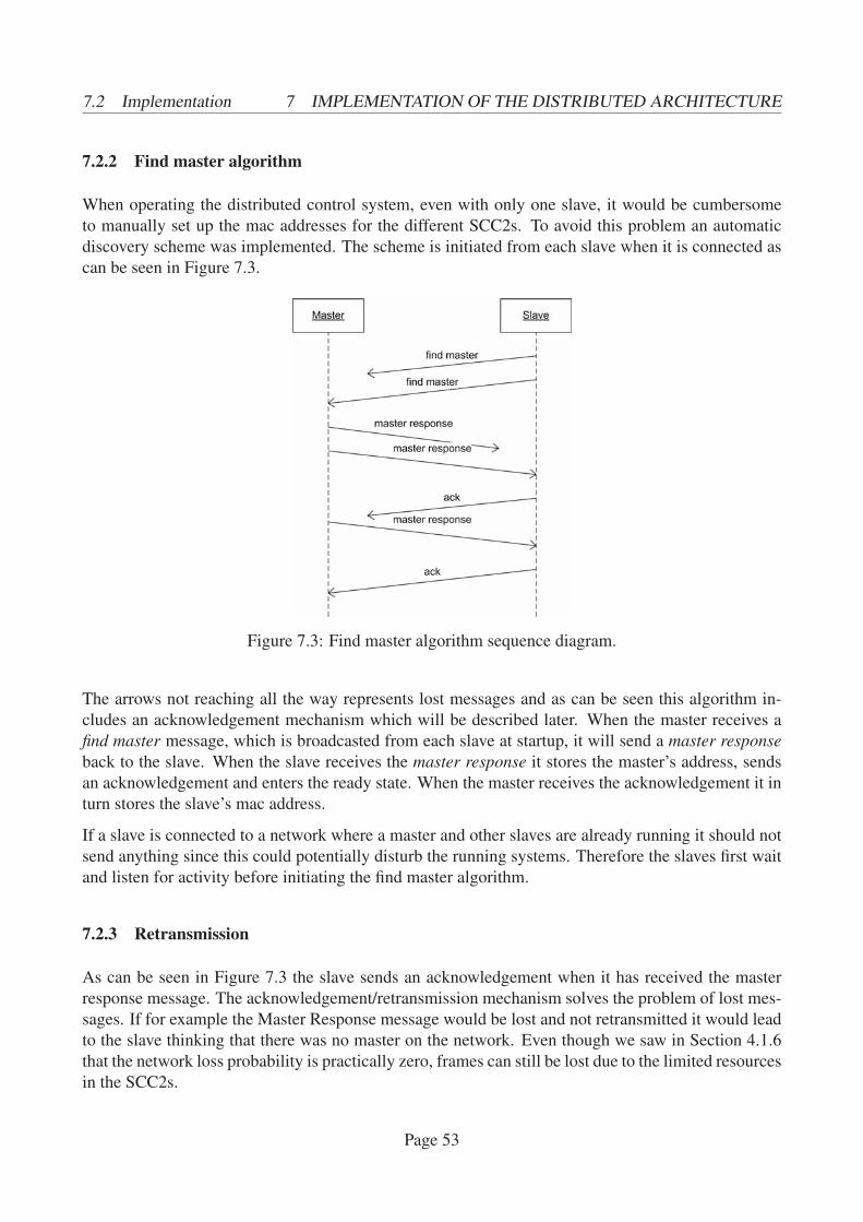
7.2 Implementation 7 IMPLEMENTATION OF THE DISTRIBUTED ARCHITECTURE
7.2.2 Find master algorithm
When operating the distributed control system, even with only one slave, it would be cumbersome
to manually set up the mac addresses for the different SCC2s. To avoid this problem an automatic
discovery scheme was implemented. The scheme is initiated from each slave when it is connected as
can be seen in Figure 7.3.
Figure 7.3: Find master algorithm sequence diagram.
The arrows not reaching all the way represents lost messages and as can be seen this algorithm in-
cludes an acknowledgement mechanism which will be described later. When the master receives a
find master message, which is broadcasted from each slave at startup, it will send a master responseback to the slave. When the slave receives the master response it stores the master’s address, sends
an acknowledgement and enters the ready state. When the master receives the acknowledgement it in
turn stores the slave’s mac address.
If a slave is connected to a network where a master and other slaves are already running it should not
send anything since this could potentially disturb the running systems. Therefore the slaves first wait
and listen for activity before initiating the find master algorithm.
7.2.3 Retransmission
As can be seen in Figure 7.3 the slave sends an acknowledgement when it has received the master
response message. The acknowledgement/retransmission mechanism solves the problem of lost mes-
sages. If for example the Master Response message would be lost and not retransmitted it would lead
to the slave thinking that there was no master on the network. Even though we saw in Section 4.1.6
that the network loss probability is practically zero, frames can still be lost due to the limited resources
in the SCC2s.
Page 53
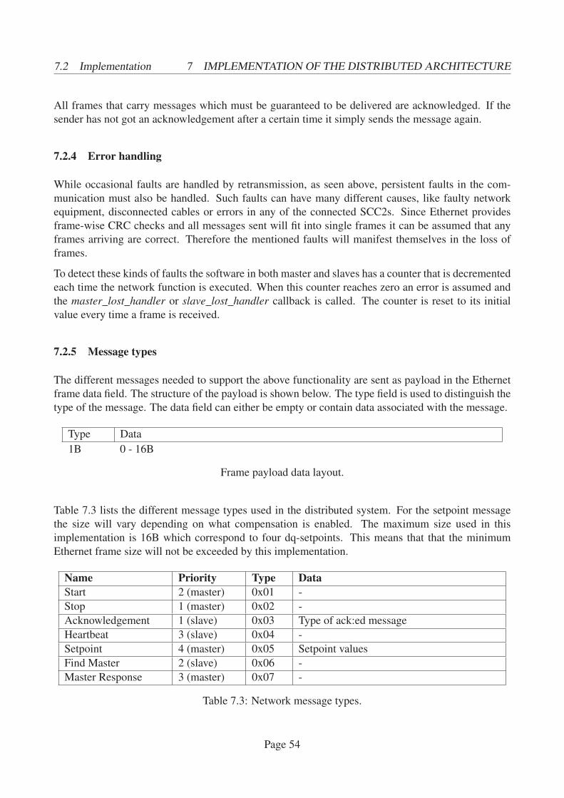
7.2 Implementation 7 IMPLEMENTATION OF THE DISTRIBUTED ARCHITECTURE
All frames that carry messages which must be guaranteed to be delivered are acknowledged. If the
sender has not got an acknowledgement after a certain time it simply sends the message again.
7.2.4 Error handling
While occasional faults are handled by retransmission, as seen above, persistent faults in the com-
munication must also be handled. Such faults can have many different causes, like faulty network
equipment, disconnected cables or errors in any of the connected SCC2s. Since Ethernet provides
frame-wise CRC checks and all messages sent will fit into single frames it can be assumed that any
frames arriving are correct. Therefore the mentioned faults will manifest themselves in the loss of
frames.
To detect these kinds of faults the software in both master and slaves has a counter that is decremented
each time the network function is executed. When this counter reaches zero an error is assumed and
the master_lost_handler or slave_lost_handler callback is called. The counter is reset to its initial
value every time a frame is received.
7.2.5 Message types
The different messages needed to support the above functionality are sent as payload in the Ethernet
frame data field. The structure of the payload is shown below. The type field is used to distinguish the
type of the message. The data field can either be empty or contain data associated with the message.
Type Data
1B 0 - 16B
Frame payload data layout.
Table 7.3 lists the different message types used in the distributed system. For the setpoint message
the size will vary depending on what compensation is enabled. The maximum size used in this
implementation is 16B which correspond to four dq-setpoints. This means that that the minimum
Ethernet frame size will not be exceeded by this implementation.
Name Priority Type DataStart 2 (master) 0x01 -
Stop 1 (master) 0x02 -
Acknowledgement 1 (slave) 0x03 Type of ack:ed message
Heartbeat 3 (slave) 0x04 -
Setpoint 4 (master) 0x05 Setpoint values
Find Master 2 (slave) 0x06 -
Master Response 3 (master) 0x07 -
Table 7.3: Network message types.
Page 54

7.3 Summary 7 IMPLEMENTATION OF THE DISTRIBUTED ARCHITECTURE
7.3 Summary
In this section a network protocol was designed to support the operation of the distributed system
over an Ethernet network. The protocol includes basic functionality to start and stop the system and
to send setpoint data.
The network functionality was implemented as a layer between the already existing network driver
and the control code.
To avoid the work of configuring the network parameters (like MAC address and number of slaves)
each time the system is run, functions that automate this were also implemented.
Since it has been observed in Section 7.2.3 that frames can be lost, functionality for acknowledgement
and retransmission of important messages was implemented. The system can also detect if a fault
condition occurs, such as network equipment failure, and take appropriate action.
Page 55
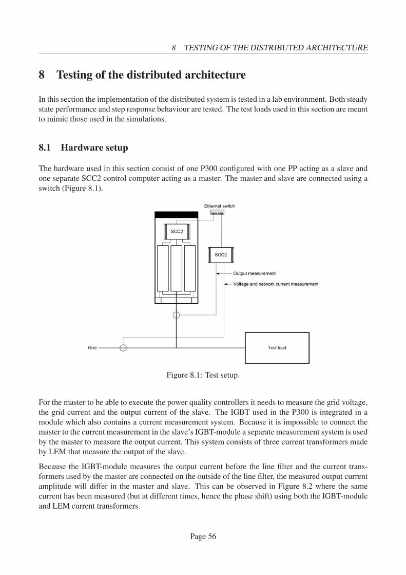
8 TESTING OF THE DISTRIBUTED ARCHITECTURE
8 Testing of the distributed architecture
In this section the implementation of the distributed system is tested in a lab environment. Both steady
state performance and step response behaviour are tested. The test loads used in this section are meant
to mimic those used in the simulations.
8.1 Hardware setup
The hardware used in this section consist of one P300 configured with one PP acting as a slave and
one separate SCC2 control computer acting as a master. The master and slave are connected using a
switch (Figure 8.1).
Figure 8.1: Test setup.
For the master to be able to execute the power quality controllers it needs to measure the grid voltage,
the grid current and the output current of the slave. The IGBT used in the P300 is integrated in a
module which also contains a current measurement system. Because it is impossible to connect the
master to the current measurement in the slave’s IGBT-module a separate measurement system is used
by the master to measure the output current. This system consists of three current transformers made
by LEM that measure the output of the slave.
Because the IGBT-module measures the output current before the line filter and the current trans-
formers used by the master are connected on the outside of the line filter, the measured output current
amplitude will differ in the master and slave. This can be observed in Figure 8.2 where the same
current has been measured (but at different times, hence the phase shift) using both the IGBT-module
and LEM current transformers.
Page 56

8.2 ADF Settings 8 TESTING OF THE DISTRIBUTED ARCHITECTURE
Figure 8.2: Output current measurement. Above: Slave, Below: Master
8.2 ADF Settings
The ADF allows for the level of compensation to be configured individually for each harmonic. For
reactive power it is possible to configure the target cosϕ.
The settings used during the measurements in this sections is presented in Table 8.1.
Setting ValueTarget cosϕ 0.97
H5 100%
H25 100%
H49 100%
Table 8.1: ADF Settings used during measurements.
8.3 Test loads
To evaluate the implemented system a number of test loads have been used. Ideally these test loads
should be similar to the loads used in the simulation but this is hard to accomplish. There was for
example no easy way to create an unbalanced load. Flicker was also not possible to generate in these
tests.
To be able to create steps in the load a three phase contactor was used. Unfortunately it was not
possible to easily synchronize the closing of the contactor in such a way that the load was connected
Page 57
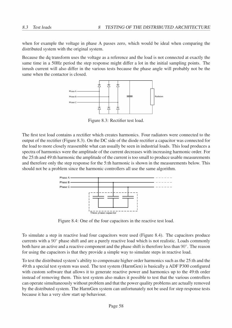
8.3 Test loads 8 TESTING OF THE DISTRIBUTED ARCHITECTURE
when for example the voltage in phase A passes zero, which would be ideal when comparing the
distributed system with the original system.
Because the dq transform uses the voltage as a reference and the load is not connected at exactly the
same time in a 50Hz period the step response might differ a lot in the initial sampling points. The
inrush current will also differ in the various tests because the phase angle will probably not be the
same when the contactor is closed.
Figure 8.3: Rectifier test load.
The first test load contains a rectifier which creates harmonics. Four radiators were connected to the
output of the rectifier (Figure 8.3). On the DC side of the diode rectifier a capacitor was connected for
the load to more closely reassemble what can usually be seen in industrial loads. This load produces a
spectra of harmonics were the amplitude of the current decreases with increasing harmonic order. For
the 25:th and 49:th harmonic the amplitude of the current is too small to produce usable measurements
and therefore only the step response for the 5:th harmonic is shown in the measurements below. This
should not be a problem since the harmonic controllers all use the same algorithm.
Figure 8.4: One of the four capacitors in the reactive test load.
To simulate a step in reactive load four capacitors were used (Figure 8.4). The capacitors produce
currents with a 90◦ phase shift and are a purely reactive load which is not realistic. Loads commonly
both have an active and a reactive component and the phase shift is therefore less than 90◦. The reason
for using the capacitors is that they provide a simple way to simulate steps in reactive load.
To test the distributed system’s ability to compensate higher order harmonics such as the 25:th and the
49:th a special test system was used. The test system (HarmGen) is basically a ADF P300 configured
with custom software that allows it to generate reactive power and harmonics up to the 49:th order
instead of removing them. This test system also makes it possible to test that the various controllers
can operate simultaneously without problem and that the power quality problems are actually removed
by the distributed system. The HarmGen system can unfortunately not be used for step response tests
because it has a very slow start up behaviour.
Page 58
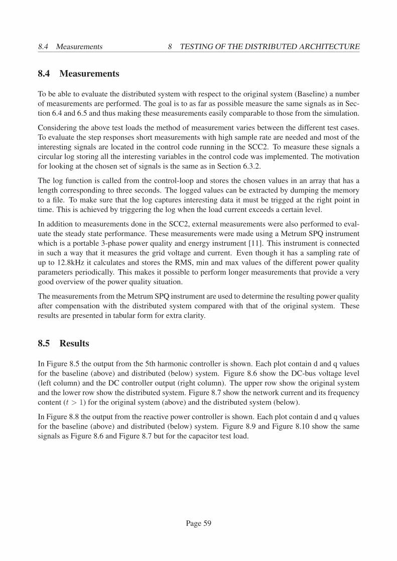
8.4 Measurements 8 TESTING OF THE DISTRIBUTED ARCHITECTURE
8.4 Measurements
To be able to evaluate the distributed system with respect to the original system (Baseline) a number
of measurements are performed. The goal is to as far as possible measure the same signals as in Sec-
tion 6.4 and 6.5 and thus making these measurements easily comparable to those from the simulation.
Considering the above test loads the method of measurement varies between the different test cases.
To evaluate the step responses short measurements with high sample rate are needed and most of the
interesting signals are located in the control code running in the SCC2. To measure these signals a
circular log storing all the interesting variables in the control code was implemented. The motivation
for looking at the chosen set of signals is the same as in Section 6.3.2.
The log function is called from the control-loop and stores the chosen values in an array that has a
length corresponding to three seconds. The logged values can be extracted by dumping the memory
to a file. To make sure that the log captures interesting data it must be trigged at the right point in
time. This is achieved by triggering the log when the load current exceeds a certain level.
In addition to measurements done in the SCC2, external measurements were also performed to eval-
uate the steady state performance. These measurements were made using a Metrum SPQ instrument
which is a portable 3-phase power quality and energy instrument [11]. This instrument is connected
in such a way that it measures the grid voltage and current. Even though it has a sampling rate of
up to 12.8kHz it calculates and stores the RMS, min and max values of the different power quality
parameters periodically. This makes it possible to perform longer measurements that provide a very
good overview of the power quality situation.
The measurements from the Metrum SPQ instrument are used to determine the resulting power quality
after compensation with the distributed system compared with that of the original system. These
results are presented in tabular form for extra clarity.
8.5 Results
In Figure 8.5 the output from the 5th harmonic controller is shown. Each plot contain d and q values
for the baseline (above) and distributed (below) system. Figure 8.6 show the DC-bus voltage level
(left column) and the DC controller output (right column). The upper row show the original system
and the lower row show the distributed system. Figure 8.7 show the network current and its frequency
content (t > 1) for the original system (above) and the distributed system (below).
In Figure 8.8 the output from the reactive power controller is shown. Each plot contain d and q values
for the baseline (above) and distributed (below) system. Figure 8.9 and Figure 8.10 show the same
signals as Figure 8.6 and Figure 8.7 but for the capacitor test load.
Page 59
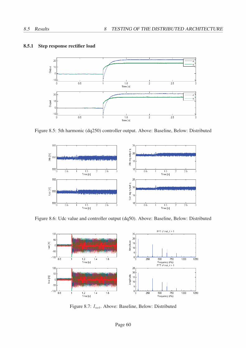
8.5 Results 8 TESTING OF THE DISTRIBUTED ARCHITECTURE
8.5.1 Step response rectifier load
Figure 8.5: 5th harmonic (dq250) controller output. Above: Baseline, Below: Distributed
Figure 8.6: Udc value and controller output (dq50). Above: Baseline, Below: Distributed
Figure 8.7: Inet. Above: Baseline, Below: Distributed
Page 60
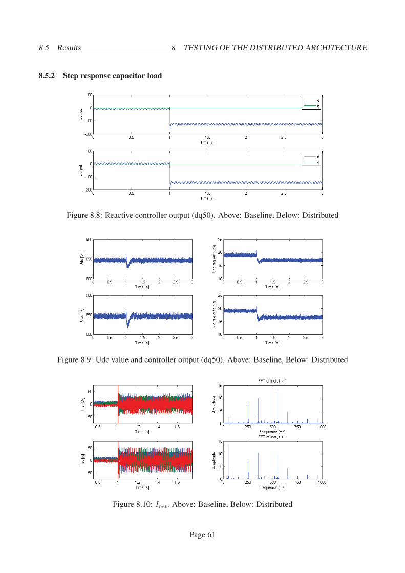
8.5 Results 8 TESTING OF THE DISTRIBUTED ARCHITECTURE
8.5.2 Step response capacitor load
Figure 8.8: Reactive controller output (dq50). Above: Baseline, Below: Distributed
Figure 8.9: Udc value and controller output (dq50). Above: Baseline, Below: Distributed
Figure 8.10: Inet. Above: Baseline, Below: Distributed
Page 61

8.5 Results 8 TESTING OF THE DISTRIBUTED ARCHITECTURE
8.5.3 Steady state
H5 Uncompensated [A] Baseline [A] Distributed [A]
phase amin 24.05 0.57 0.55
max 24.36 0.77 0.74
phase bmin 23.46 0.65 0.65
max 23.72 0.79 0.78
phase cmin 23.60 0.50 0.55
max 23.78 0.63 0.70
Table 8.2: 5th harmonic min/max values during measurement.
H25 Uncompensated [A] Baseline [A] Distributed [A]
phase amin 18.69 0.50 0.55
max 18.90 0.68 0.63
phase bmin 18.04 0.58 0.55
max 18.26 0.75 0.70
phase cmin 18.35 0.53 0.56
max 18.65 0.78 0.73
Table 8.3: 25th harmonic min/max values during measurement.
H49 Uncompensated [A] Baseline [A] Distributed [A]
phase amin 13.52 0.56 0.55
max 13.71 0.85 0.79
phase bmin 13.08 0.66 0.65
max 13.22 0.82 0.73
phase cmin 12.93 0.48 0.46
max 13.19 0.56 0.53
Table 8.4: 49th harmonic min/max values during measurement.
Q Uncompensated [kVAr] Baseline [kVAr] Distributed [kVAr]
phase amin 9.88 0.83 0.62
max 10.01 1.04 0.82
phase bmin 9.75 0.45 0.17
max 9.90 0.61 0.34
phase cmin 9.68 0.75 0.55
max 9.87 0.87 0.68
Table 8.5: Reactive Power (Q) min/max values during measurement.
Page 62

8.6 Analysis 8 TESTING OF THE DISTRIBUTED ARCHITECTURE
8.6 Analysis
Generally the results produced in this section are comparable to those in the simulation. There are
of course a lot of measurement noise, especially in the Inet measurement, but this was expected. An
unbalanced test load was used in the simulations but it was not available in the lab environment. A
source of flicker was also not available in the lab. For the loads that could be replicated it was still
hard to generate reproducible measurements of the step responses.
As explained in Section 8.1 and seen in Figure 8.2 the measurement of the output current differs
between the master and the slave. This difference is caused by the need to use both different measure-
ment equipment and a different measurement point for the master. These problems are purely caused
by limitations in the test setup and has nothing to do with the design of the distributed system.
Looking at the setpoint for the 5th harmonic controller (Figure 8.5) during a step response shows that
the differences between the original system and the distributed system are very small. The rectifier
load produces a spectrum of harmonics and only the 5th, 25th and 49th are removed. Therefore Inetwill still contain the remaining harmonics as in seen in Figure 8.7. This figure also contain Fast
Fourier Transform (FFT) spectrums for Inet and there it can clearly be seen that the compensated
harmonics are not present.
Table 8.2, 8.3 and 8.4 show the remaining current for each harmonic during the steady state mea-
surement. The distributed system performs as good as the original systems for each of the three
harmonics.
For the capacitor load step response there are two major differences between the setpoint graph for
the original system and the distributed system. For the original system (Figure 8.8) it can be seen that
the setpoint oscillates slightly below zero before the load is connected while it is centered around zero
in the distributed system.
This difference is caused by the fact that the reactive power controller uses the load current, which is
calculated as the difference of the grid and output current. When measuring the output current outside
of the line filter, which is the case for the master in the distributed system, the measured current will
contain a component corresponding to the current caused by the line filter. This component is also
present in the grid current measurement. Therefore this current will cancel itself out and the setpoint
will be zero before the load is connected.
This phenomenon has also been observed in simulations of the original system when the measurement
point has been moved to the outside of the line filter.
The other difference between the original and distributed system is that the final value after the step is
different. This can be explained by the amplitude difference in the measured output current observed
earlier. This difference will cause the ADF to output a compensation current with incorrect amplitude.
This can be seen in the FFT spectrum in Figure 8.10 were this excessive current appear as a 50Hz
component.
For the steady state reactive power tests it was only possible to generate either −90◦ or 90◦ phase
shift of the base current and nothing in between. Since this means that only a reactive current will be
generated there will only be noise left after reactive power compensation.
Ideally the steady state reactive power results should be presented as cosϕ quantities and be compared
Page 63

8.7 Summary 8 TESTING OF THE DISTRIBUTED ARCHITECTURE
to the actual setting of the ADF. However cosϕ become inaccurate when no active current is flowing.
Therefore the amount of reactive power is instead shown in Table 8.5. Even if it is not possible to see
the exact cosϕ value it is evident that most of the reactive power is removed by both the original and
distributed system.
For both the rectifier and capacitor test load it can be seen in Figure 8.6 and Figure 8.9 that the Udc
level and control setpoint is unaffected by the introduction of a distributed architecture.
8.7 Summary
The tests conducted in this section show that the distributed system performs as expected from the
simulations. Harmonic compensation is the same in the distributed system as in the original sys-
tem. Reactive compensation differs slightly but it is shown that this difference can be explained by
properties of the test setup, the primary difference being how the output current is measured.
Page 64

9 DISCUSSION AND CONCLUSION
9 Discussion and conclusion
The purpose of this master’s thesis was to investigate if it was possible to divide the control tasks in the
ADF P300 in such a way that the system could be distributed over an Ethernet network. By thorough
investigations of the original lab system a suitable design was found and tested both in simulations
and in real world environments. The results of these tests have shown that there is a negligible impact
on performance in the distributed system. The highest harmonic that is possible to compensate has
not been affected negatively and the response time of the system is only marginally affected.
It has been shown through both studies of the involved technologies, such as Ethernet, and through
a number of tests that the distributed system fulfils the requirements identified in Section 5.4. Since
Ethernet performs a CRC check for each frame, corrupted data should not be delivered to the control
application. The system also features acknowledgement of important frames and detection of per-
sistent faults in the communication. A few lost setpoint frames will only lead to a slight, temporary
reduction in compensation performance since the slave will just keep using the old setpoint. These
features make the system robust and fault tolerant.
Of course many things could be improved or could have been done differently. The network driver
used is probably not implemented with real-time performance in mind. It uses a lot of execution time
and imposes unnecessary long delays. By measuring the execution time for the different controllers
and network functions it was deducted that it would not be possible to have everything running at
once. The solution to this was to simply disable things that was not needed for the experiments in this
thesis. Also since it was hard to obtain a test load that caused flicker the parts of the system handling
flicker was not tested at all.
Unfortunately the distributed system design proposed in this thesis has little practical use. This is
primarily due to the fact that it contains a single point of failure: the master SCC2. An important
further improvement would be to remove this weakness by modifying the current design to allow any
SCC2 to be master. The main challenge in achieving this consist of finding a way to transmit and
combine the output current measurement from the slaves. Also fault tolerant algorithms for deciding
which SCC2 should be master are needed.
As mentioned before the switch ripple is an unwanted product of the ADF. Another improvement for
the distributed system would be to add functionality that can coordinate the switching of the ADFs.
By using the 50Hz voltage as a timing reference the different systems could be synchronized in such
a way that their switch ripple currents cancel each other out.
The current design should only be seen as a proof of concept that the P300 control algorithms can in
fact be successfully distributed over a switched Ethernet network with existing SCC2 hardware.
Page 65
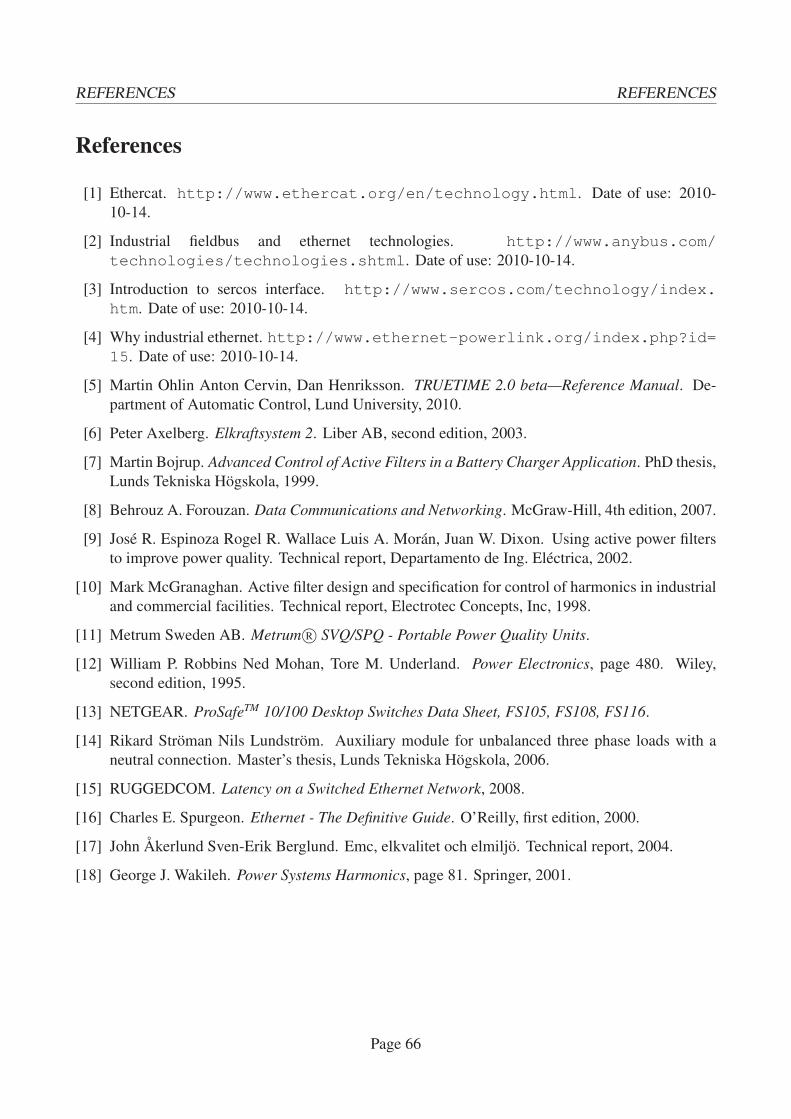
REFERENCES REFERENCES
References
[1] Ethercat. http://www.ethercat.org/en/technology.html. Date of use: 2010-
10-14.
[2] Industrial fieldbus and ethernet technologies. http://www.anybus.com/technologies/technologies.shtml. Date of use: 2010-10-14.
[3] Introduction to sercos interface. http://www.sercos.com/technology/index.htm. Date of use: 2010-10-14.
[4] Why industrial ethernet. http://www.ethernet-powerlink.org/index.php?id=15. Date of use: 2010-10-14.
[5] Martin Ohlin Anton Cervin, Dan Henriksson. TRUETIME 2.0 beta—Reference Manual. De-
partment of Automatic Control, Lund University, 2010.
[6] Peter Axelberg. Elkraftsystem 2. Liber AB, second edition, 2003.
[7] Martin Bojrup. Advanced Control of Active Filters in a Battery Charger Application. PhD thesis,
Lunds Tekniska Högskola, 1999.
[8] Behrouz A. Forouzan. Data Communications and Networking. McGraw-Hill, 4th edition, 2007.
[9] José R. Espinoza Rogel R. Wallace Luis A. Morán, Juan W. Dixon. Using active power filters
to improve power quality. Technical report, Departamento de Ing. Eléctrica, 2002.
[10] Mark McGranaghan. Active filter design and specification for control of harmonics in industrial
and commercial facilities. Technical report, Electrotec Concepts, Inc, 1998.
[11] Metrum Sweden AB. Metrum R© SVQ/SPQ - Portable Power Quality Units.
[12] William P. Robbins Ned Mohan, Tore M. Underland. Power Electronics, page 480. Wiley,
second edition, 1995.
[13] NETGEAR. ProSafeTM 10/100 Desktop Switches Data Sheet, FS105, FS108, FS116.
[14] Rikard Ströman Nils Lundström. Auxiliary module for unbalanced three phase loads with a
neutral connection. Master’s thesis, Lunds Tekniska Högskola, 2006.
[15] RUGGEDCOM. Latency on a Switched Ethernet Network, 2008.
[16] Charles E. Spurgeon. Ethernet - The Definitive Guide. O’Reilly, first edition, 2000.
[17] John Åkerlund Sven-Erik Berglund. Emc, elkvalitet och elmiljö. Technical report, 2004.
[18] George J. Wakileh. Power Systems Harmonics, page 81. Springer, 2001.
Page 66