research article distributed control design for...

Research ArticleDistributed Control Design for Structures Subjected toTraveling Loads

Dominik Pisarski

Institute of Fundamental Technological Research (IPPT) Polish Academy of Sciences Pawinskiego 5b 02-106 Warsaw Poland

Correspondence should be addressed to Dominik Pisarski dpisaripptpanpl

Received 28 July 2015 Accepted 13 September 2015

Academic Editor Qingling Zhang

Copyright copy 2015 Dominik Pisarski This is an open access article distributed under the Creative Commons Attribution Licensewhich permits unrestricted use distribution and reproduction in any medium provided the original work is properly cited

This paper presents a novel distributed control method that adapts the structures subjected to traveling loads The adaptation isrealized by changes of the damping of the structurersquos supports The control objective is to provide smooth passage of vehicles andto extend the safe life-time of the carrying structures The results presented in the previous works of the author exhibited highperformance of supports with an open-loop switching damping policy In this paper the goal is to develop a state feedback strategythat is significantly less sensitive to the system parameters and much simpler for practical implementation Further efforts are putinto designing a distributed controller architecture where only the local and the relevant neighboring states are used to computethe control decisions The proposed controller is validated experimentally It exhibits high performance in a wide range of travelspeeds The practicality of the proposed solution should attract the attention of practicing engineers

1 Introduction

Problems of structures subjected to loads traveling withhigh velocity are of special interest for practicing engineersNumerous analytic and numerical solutions are being appliedto solve the problems of transportation and robotic systemswith single or multipoint interactions such as train-trackvehicle-bridge or effector-guidewayThese problems concernthe high vibration levels of both the structures and thetraveling objects due to continually increasing speeds andload carrying capacity requirements The construction ofnew railway tracks or bridges with a sufficiently higher loadcarrying capacity and ability to withstand dynamical stressesand strains is usually limited by costs On the other hand astatic strengthening increases the structurersquosmass and is oftenrestricted for technological reasons To face the undesiredvibration effects a variety of control systems acting on boththe structures and the suspension of the traveling loads havebeen proposed and put into practice

A common objective in structural control is to enhancethe stability of the systems subjected to impulsive or periodicexcitation The first group of control methods referred to asthe active methods is based on force actuators An active

controlmethod to control the beam vibrations via linear forceactuators is presented for example in [1] A similar controlproblem adapting a piezoelectric layer was considered in[2] An actively controlled beam subjected to a harmonicexcitation was presented in [3] An actively controlled stringsystem was considered in [4] Interesting results on thecontrol of a cantilever beam by the use of electromagneticactuators can be found in [5] In the active methods instructural control we can also include the control of thetrackrsquos shape In [6] the authors developed an approach thatuses active smart sleepers that enable the track to shift upand down The objective was to minimize the deflection ofthe track In [7] the authors suggested an active controlmethod based on the linear quadratic regulator to suppressthe vibration of bridges

A recent trend is to replace force actuators with semiac-tivemagnetorheological dampersThese solutions are usuallyless efficient However they attract engineersrsquo interest due totheir significantly lower power consumption They are alsosafer in the case of a control system failure Unlike activesystems the semiactive ones based on controlled damperscan be always switched to passive mode providing systemstability One of the first concepts of the semiactive control

Hindawi Publishing CorporationMathematical Problems in EngineeringVolume 2015 Article ID 206870 12 pageshttpdxdoiorg1011552015206870

2 Mathematical Problems in Engineering

in mechanical systems was proposed by Karnopp Crosbyand Harwood In [8] they presented the idea of stabilizingof the oscillator with one degree of freedom moving uponuneven ground The algorithm developed by the authorsldquoSkyhookrdquo is today one of the most widely used ones insuspension control systems for vehiclesThe idea was initiallydesigned to improve the comfort of passengers Later similarcontrol method was adopted to the oscillator moving uponcarrying structures Extensive results were demonstratedin [9 10] Controlled dampers are incorporated also forseismic isolation Interesting results can be found in [11 12]In [13] the authors proposed to control both the stiffnessand damping parameters The control decision led to themaximum dissipation of energy

The use of semiactive supports for a structure subjectedto a moving load was first proposed in [14] By means ofnumerical simulations the authors demonstrated that for awide range of travel velocities switching damping strategiesoutperform standard passive solutions The idea was laterextended in [15 16] where by introducing a rigorous analysisand optimization techniques the authors concluded that evenone switching action for each damper can provide verysmooth load passages A metric corresponding to the totaldeflection of the load trajectory from the desired straightline was reduced by up to 50 percent The drawbacks ofthe proposed method lie in its complicated implementationand high sensitivity to system uncertainties As the authorsdemonstrated in order to provide a desired performanceopen-loop switched solutions need to be recomputed everytime we expect a different travel speed

This paper proposes a novel control method to reduce thevibration levels of carrying structures subjected to movingloads The method is dedicated to the applications to largescale structures like bridges and overpasses subjected totraveling trains as well as to robotic guideways subjected toeffectors performing technological processes for examplecutting bonding or painting The control objective is toprovide a smooth passage of the traveling load and to extendthe safe life-time of the carrying structures The proposedcontrol strategy is based on the optimal centralized open-loop solutions presented in [15 16] but due to a distributedcontroller architecture and a state feedback control law it is alot more practical and robust

For the distributed controller we will impose the fol-lowing requirements functional symmetry in the controllerrsquosstructure theminimumcomputational burden and informa-tion exchange The symmetry will be achieved by splittingthe controller intomodules realizing the same computationalprocedures The modular type of architecture is convenientfor system assembly and maintenance Each of the moduleswill compute its control decision by using local state informa-tion and the average state of the whole structure The aver-age state will be reconstructed by exchanging informationbetween the neighboring controllers The final tuning of thecontroller was done by solving a corresponding optimizationproblem Then a series of experiments on a physical modelof a controlled guideway was performed As will be demon-strated the proposed controlmethod provides a performance

l

w

0

0 x

m

middot middot middot

xm(t)

(t)

km

am

um

EI 120583

k1

a1

u1 k2

a2

u2

Figure 1 A span supported by set of controlled dampers andsubjected to a mass travelling at speed V(119905)

that is comparable with the optimal centralized solutions andit is robust to changes in the speed of the traveling load

The rest of this paper is structured as follows A math-ematical model of a carrying structure supported with a setof controlled dampers and subjected to a traveling load ispresented in Section 2 Section 3 introduces the distributedcontroller architecture and defines the local control lawsThe distributed averaging problem is studied in Section 4 InSection 5 an explicit procedure for the controller implemen-tation is given In Section 6 a method for finding an optimalparameter of the controller is presented Finally the resultsof experimental tests of the performance of the designedcontroller will be presented in Section 7

2 Investigated System

In this section we will introduce a mathematical represen-tation of a carrying structure supported by set of controlleddampers illustrated in Figure 1 This representation will beused in the final tuning of the proposed controller (seeSection 6)

For themodel of the span we will use the Euler-Bernoullibeam equation which is broadly applied to thin elastic bodiessubjected to small deflections A beam of the total length 119897is characterized by the bending stiffness 119864119868 and density perunit length 120583 A set of controlled supports are located at thepositions 119886

119894 For each of the supports we assume a controlled

damping 119906119894andor a fixed stiffness 119896

119894 The beam is subjected

to a mass 119898 travelling at the time-varying velocity V = V(119905)that is assumed to be given Position of the mass is denotedby 119909119898(119905) and computed by using

119909119898 (119905) = int

119905

0

V (119905) 119889119905 (1)

Denoting the transverse deflection of the span by 119908(119909 119905) thesystem is governed by

1198641198681205974119908 (119909 119905)

1205971199094+ 120583

1205972119908 (119909 119905)

1205971199052

= minus

119898

sum119894=1

(119896119894119908 (119886119894 119905) + 119906

119894

120597119908 (119886119894 119905)

120597119905) 120575 (119909 minus 119886

119894)

minus 119898(119892 +1205972119908 (119909119898 (119905) 119905)

1205971199052)120575 (119909 minus 119909

119898 (119905))

(2)

Mathematical Problems in Engineering 3

The endpoint supports impose the following boundary con-ditions

119908 (0 119905) = 0

119908 (119897 119905) = 0

(1205972119908

1205971199092)|119909=0

= 0

(1205972119908

1205971199092)|119909=119897

= 0

(3)

For the initial conditions we assume

119908 (119909 0) = 0

(119909 0) = 0(4)

The left-hand side of (2) consists of the standard terms of theEuler-Bernoulli equation corresponding to the potential andinertial forces of the beam The first two terms of the righthand side stand for the reactions of the controlled supportsThe last terms correspond to the excitation of the movingload For this excitation we take into account both gravityand the inertial forceThe latter is often ignored for large scalestructures For the systems where the masses of the span andmoving load are comparable (eg maglev trains robotics)the inertial force of the moving mass plays a key role in thedynamics (see [17 18])

21 ODE Representation For the sake of further studies wewill now represent (2) as a set of the ordinary differentialequations Let us first introduce the orthogonal basis

120579119895(119909) = sin(

119895120587119909

119897) 119895 = 1 2 (5)

It clearly fulfils the boundary conditions (3) For such a basisa solution of (2) can be represented as follows

119908 (119909 119905) =2

119897

infin

sum

119895=1

119881119895(119905) 120579119895(119909) (6)

By inserting (6) into (2) we obtain

2119864119868

119897

1205974

1205971199094(

infin

sum

119895=1

119881119895(119905) 120579119895(119909)) +

2120583

119897

sdot1205972

1205971199052(

infin

sum

119895=1

119881119895(119905) 120579119895(119909)) = minus

2

119897

119898

sum119894=1

119896119894

sdot

infin

sum

119895=1

119881119895(119905) 120579119895(119886119894) 120575 (119909 minus 119886

119894) minus

2

119897

sdot

119898

sum119894=1

119906119894

120597

120597119905(

infin

sum

119895=1

119881119895(119905) 120579119895(119886119894))120575 (119909 minus 119886

119894)

minus 119898[

[

119892 +1205972

1205971199052(2

119897

infin

sum

119895=1

119881119895(119905) 120579119895(119909119898 (119905)))

]

]

sdot 120575 (119909 minus 119909119898 (119905))

(7)

Now each term of (7) is multiplied by

120579119895 (119909) = sin(

119895120587119909

119897) (8)

and then integrated with respect to 119909 over the interval [0 119897]This results in the following weak formulation

2

119897

infin

sum

119895=1

[119864119868(119895120587

119897)

4

119881119895(119905) + 120583

119895(119905)]int

119897

0

120579119895(119909) 120579119895 (119909) 119889119909

= minus2

119897

119898

sum119894=1

infin

sum

119895=1

119896119894119881119895(119905) int119897

0

120579119895(119886119894) 120579119895 (119909) 120575 (119909 minus 119886119894) 119889119909

minus2

119897

119898

sum119894=1

infin

sum

119895=1

119906119894119895(119905) int119897

0

120579119895(119886119894) 120579119895 (119909) 120575 (119909 minus 119886119894) 119889119909

minus 119898119892int119897

0

120579119895 (119909) 120575 (119909 minus 119909119898 (119905)) 119889119909 minus

2119898

119897

sdot1205972

1205971199052(

infin

sum

119895=1

119881119895(119905) 120579119895(119909119898 (119905)))

sdot int119897

0

120579119895 (119909) 120575 (119909 minus 119909119898 (119905)) 119889119909

(9)

Note that (9) must hold for every 119895 = 1 2 Nowwe can usethe orthogonality condition for the 120579 functions that is

int119897

0

120579119895(119909) 120579119895 (119909) 119889119909 =

119897

2120575119895119895 (10)

Here 120575119895119895

stands for the Kronecker delta By using the siftingproperty of the Dirac delta function we can also give explicitformulas for the terms

int119897

0

120579119895(119886119894) 120579119895 (119909) 120575 (119909 minus 119886119894) 119889119909 = 120579119895 (119886119894) 120579119895 (119886119894)

int119897

0

120579119895 (119909) 120575 (119909 minus 119909119898 (119905)) = 120579119895 (119909119898 (119905))

(11)


Thus (9) can be written as follows

120583

infin

sum

119895=1

119895(119905) 120575119895119895+ 119864119868

infin

sum

119895=1

(119895120587

119897)

4

119881119895(119905) 120575119895119895

= minus2

119897

119898

sum119894=1

infin

sum

119895=1

(119896119894119881119895(119905) + 119906119894119895 (119905)) 120579119895 (119886119894) 120579119895 (119886119894)

minus 119898119892120579119895(119909119898 (119905))

minus2119898

119897

1205972

1205971199052(

infin

sum

119895=1

119881119895(119905) 120579119895(119909119898 (119905))) 120579119895 (119909119898 (119905))

119895 = 1 2

(12)

It still remains to compute the second time derivative ofsuminfin

119895=1119881119895(119905)120579119895(119909119898(119905)) An explicit formula for this derivative is

given below

1205972

1205971199052(

infin

sum

119895=1

119881119895(119905) 120579119895(119909119898 (119905)))

=

infin

sum

119895=1

119895(119905) 120579119895(119909119898 (119905))

+

infin

sum

119895=1

2119895120587

119897119895(119905) 120601119895(119909119898 (119905)) V (119905)

+

infin

sum

119895=1

119895120587

119897119881119895(119905) 120601119895(119909119898 (119905)) V (119905)

minus

infin

sum

119895=1

1198952

1205872

1198972119881119895(119905) 120579119895(119909119898 (119905)) (V (119905))

2

(13)

Here we use the notation 120601119895(119909119898(119905)) = cos(119895120587119909

119898(119905)119897)

Regarding only these terms in (12)where theKronecker deltasare not equal to zero we can finally rewrite (2) as follows

119908 (119909 119905) =2

119897

infin

sum

119895=1

119881119895(119905) 120579119895(119909)

120583119895 (119905) + 119864119868 (

119895120587

119897)4

119881119895 (119905)

= minus2

119897

119898

sum119894=1

infin

sum

119895=1

(119896119894119881119895(119905) + 119906119894119895 (119905)) 120579119895 (119886119894) 120579119895 (119886119894)

minus 119898119892120579119895(119909119898 (119905))

minus2119898

119897

infin

sum

119895=1

119895(119905) 120579119895(119909119898 (119905)) 120579119895 (119909119898 (119905))

minus4119898

119897

infin

sum

119895=1

119895120587

119897119895(119905) 120601119895(119909119898 (119905)) 120579119895 (119909119898 (119905)) V (119905)

minus2119898

119897

infin

sum

119895=1

119895120587

119897119881119895(119905) 120601119895(119909119898 (119905)) 120579119895 (119909119898 (119905)) V (119905)

+2119898

119897

infin

sum

119895=1

1198952

1205872

1198972119881119895(119905) 120579119895(119909119898 (119905)) 120579119895 (119909119898 (119905)) (V (119905))

2

119895 = 1 2

(14)

The initial condition is now given by

119881119895 (0) = 0

119895 (0) = 0

119895 = 1 2

(15)

22 State-Space Representation Control Bounds From (14)we can observe that at each time instant the state ofthe system is fully characterized by the sets 119881

119895(119905) and

119895(119905) Throughout the rest of the paper we will rely on an

approximated representation of (14) by taking 119895 from 1 to119899 = 10 The assumed ten modes are sufficient to render thedynamics of span while keeping the size of the system eligiblefor efficient optimization

By introducing the state vector 119910 isin R2119899 such that

119910 (119905)

= [1198811 (119905) 1 (119905) 1198812 (119905) 2 (119905) 119881119899 (119905) 119899 (119905)]

119879

(16)

we can represent (14) by the following time-varying bilinearsystem

119910 = 119860 (119905) 119910 +

119898

sum119894=1

119906119894119861119894 (119905) 119910 + 119865 (119905)

119910 (0) = 0

(17)

Here the matrices 119860 and 119861 are mainly built upon the eigen-functions 120601 and 120579 while the excitation vector 119865 collects theterms related to the force of gravity (for detailed structures see[19]) For the controls we assume that each one is boundedby two positive values corresponding to the minimum andmaximum admissible damping coefficients that is

119906 isin U = [119906min 119906max ]119898sub R119898

+ (18)

3 Control Design

The goal of this section is to introduce a distributed statefeedback control law for system (17) First let us characterizethe distributed controller architecture

31 Distributed Controller Architecture For each of the con-trolled supports we will now associate a local state asillustrated in Figure 2 The control decision 119906

119894 together with


um

w1 w2 w3 wm

ui = ui(t) mdashlocal control decisionSi = (wi ui)mdashlocal subsystem

u3u2u1



wi = w(ai t) (ai t) mdashlocal statew

Figure 2A controlled beam represented as a set of local subsystems

Centralcomputer

S1 S2 S3 Smmiddot middot middot

u1u2

u3um

w1w2

w3

wm

Figure 3 Centralized controller architecture The whole system ismanaged by a central computer

the associated state119908119894= 119908(119886

119894 119905) (119886

119894 119905) will be referred to

as the subsystem and be denoted by 119878119894

For such representation a centralized controller architec-ture can be visualized as shown in Figure 3 All accessiblestates are first transferred to a central computing unit Basedon the given information the unit takes a decision that issent to all control devices In a distributed architecture weassume that each of the local subsystems is managed by itsown computing unit as depicted in Figure 4That practicallymeans that every local computer is allowed to measure onlyits local state and send a control signal to a correspondinglocal control device Note that due to the coupled dynamicseach of the local decisions affects the whole system Thusa controller relying only on the local states may lead toundesired states To improve performance and to providerobustness a distributed controller allows local computers toexchange some information In our setting we assume thatcomputers 1 to119898minus1 send their state information to their rightneighbors while computer119898 delivers the state to computer 1The assumed communication topology will be later used forsolving the distributed averaging problem

The proposed distributed architecture is modular and hasfunctional symmetry that is each of the local controllerscan be seen as a module realizing the same procedure Thistype of architecture is convenient for system assembly andmaintenance in particular for large scale structures In thecase of failure only the malfunctioning module needs to bereplaced In addition such a modular decentralization playsan important role in safety Suppose there is a malfunctionof the central computer An incorrect signal is then sentto the whole system In a modular controller architecturethis risk is reduced to local failures For an executive com-ponent of a proposed module one can consider a rotarymagnetorheological damper equipped with an encoder (seehttpwwwlordcom)

Local

u1 u2 u3 umw1w1 w2

w2 w3w3

wm

wm

wmminus1

computerLocal

computerLocal

computerLocal

computer



Figure 4Distributed controller architectureThe system is operatedby a set of local computers allowed to exchange state information

32 Distributed Control Law Under the assumed distributedarchitecture wewill nowdesign a control law to be performedby each of the local controllers The first requirement is thatthis control law is based on the accessible state informationand can be implemented in real-time We also require thatthe resulting closed-loop system is robust in the sense that itis not sensitive to small changes of the system parameters inparticular changes in the velocity of the moving load This isof special importance for structures subjected to vehicles forwhich we can naturally expect various speeds The commoncontrol objective is to reduce the vibration levels of thestructure as well as to provide a smooth straight line passagefor the traveling load

The control law introduced in this work is heuristicHowever it arises from the analysis on the system dynamicsas well as the optimal solutions studied in [15 16 19 20] Theidea of a straight line passage is based on the fundamentalprinciple of a two-sided lever In Figure 5 we illustrate thisidea for a beam supported by two controlled dampers Duringthe first stage of a passage for the left damper we setits maximum admissible damping value providing that thedeflection under a moving load maintains moderate levelsAt the same time the damper on the right operates at itsminimum value enabling a beam to turn around its centerof gravity and to lever its right hand part This temporalincrement of displacement of the right hand part results ina nearly straight line load trajectory during the second stageof the passage when the operation modes of the dampers arereversed

Formally the problem of an optimally straight line pas-sage for system (17) can be written as follows

find 119906lowast = argmin119906isinU

119869 = int119879

0

119910119879119876 (119905) 119910 119889119905

under 119910 = 119860 (119905) 119910 +

119898

sum119894=1

119906119894119861119894 (119905) 119910 + 119865 (119905)

(19)

Here the time horizon119879 is equal to the total time of a passageand is computed by using

119897 = int119879

0

V (119905) 119889119905 (20)

The matrix 119876(119905) is taken such that

119910119879119876 (119905) 119910 = (119908 (V119905 119905))2 (21)


u1 = umax u2 = umin u2 = umaxu1 = umin

Figure 5 The idea of a straight line passage based on the principle of a two-sided lever

u1(t)

u2(t)

u3(t)

um(t)

0 1205911 1205912 1205913 120591m tf t

umaxumin

Figure 6 Diagonal structure of the optimal controls for straight linepassage of a moving load

Thus the objective function corresponds to the total deflec-tion of the trajectory of a moving load

A comprehensive study of a solution to problem (19)was presented in [19] The author demonstrated that for awide range of systemparameters the solutions exhibit similarstructures This structure is represented by the diagonalpattern depicted in Figure 6 Here 120591

119894stands for the time

instant in which a traveling load is passing the position 119886119894

The practical meaning of this pattern is that each damper issupposed to be switched to the maximum admissible valuejust before the load approaches it while the switch back tothe minimum value is supposed to be done right after thatpassage In this paper we will design a state feedback controllaw that mimics the optimal diagonal pattern providing alsorobustness to a wide range of travel speedThe key in derivingthis control law is the observation of how the state of a beamcorresponds to the horizontal position of a moving load

Suppose that for the beam presented in Figure 2 we puttwo observersThe first one focuses on the transverse velocityof the point 119886

1 that is (119886

1 119905) while the other collects

the transverse velocities for all points 119886119894and computes the

average of the absolute values (1119898)sum119898119894=1|(119886119894 119905)| On the

left hand side of Figure 7 an approximate evolution of (1198861 119905)

during the passage is depicted We can observe that thelocal transverse velocity reaches its highest negative valueswhen the moving load is in the neighborhood of the position1198861 Then it slowly changes sign and 119886

1returns toward the

equilibrium A similar behavior can be observed over a widerange of passage speeds with the tendency that a larger speedmagnifies the trajectory (If the local observer is located atthe position 119886

119894 then the trajectory is analogous except for

the convex part that is shifted to 120591119894) The second observer

notices that the average (1119898)sum119898119894=1|(119886119894 119905)| rapidly increases

and remains at some level up to the end of the passage (seethe right-hand side of Figure 7) A similar result is also validfor different passage velocities with the tendency that largerspeeds magnify the trajectory Our task now is to reconstruct

the desired control action denoted by the dotted lines withthe use of the measurements by both observers The readercan verify that this action can be approximately provided bythe following control law

119906119894 (119905) =

119906max if (119886119894 119905) le minus120572

1

119898

119898

sum119894=1

1003816100381610038161003816 (119886119894 119905)1003816100381610038161003816

119906min otherwise(22)

Here 120572 gt 0 The control law states that we are supposed to setthe maximum control value only when the local transversevelocity is below the bound given by the average absolutevalue (more precisely some portion of this average wherethe portion is determined by the constant parameter 120572)The role of the average is to adapt the switching bound todifferent passage speeds From Figure 7 one can notice thatif we relied on some fixed switching bound then the controlsmay operate on the maximum values either too shortly (forslow passages) or too long (in case of fast travels)

The controller given by (22) is supposed to be imple-mented with the information allowed by the distributedarchitecture (Figure 4) While the local state is assumed tobe given the average needs to be computed in a distributedmanner with the use of the circular information exchangebetween the local computers The problem of distributedaveraging will be studied in the next section The method forselecting the parameter 120572 will be presented in Section 6

4 Distributed Averaging Problem

The controller given by (22) is supposed to be implementedwith the information allowed by the distributed architecture(Figure 4) While the local state is assumed to be given theaverage needs to be computed in a distributed manner withthe use of the circular information exchange between thelocal computers Before we give an algorithm for distributedaveraging let us first introduce a relevant background Wewill now consider a linear dynamical system

119911 (119896 + 1) = 119860119911 (119896) 119896 = 0 1

119911 (0) = 1199110 119911 isin R119899

(23)

The distributed averaging problem is formulated as followsFind the matrix 119860 such that the state of system (23)

converges to a common value that is equal to the average ofthe initial state

A system solving the distributed averaging problem is aparticular case of the consensus protocols A comprehensivetheoretical framework for consensus problems can be found


ttf1205911ttf1205911

w(a1 t) (1m)sum m

i=1| (ai t)|

12

12

w

Figure 7 Evolution of the local transverse velocity (1198861 119905) and the average of the absolute values of the local transverse velocities

(1119898)sum119898

119894=1|(119886119894 119905)| for two different moving load speeds V

1lt V2 Dotted lines mark the desired shape for control 119906

1

in [21] Here we will present only the fundamental results fordistributed averaging under linear dynamics

Let 119888 be a real number We say that system (23) solvesthe consensus problem (or that system (23) is a consensusprotocol) if and only if there exists an asymptotically stableequilibrium 119911

lowast satisfying

119911lowast= 1198881 (24)

where 1 stands for the all-ones vector A necessary andsufficient condition for system (23) to be a consensusprotocol is that 119860 has 1 as a simple eigenvalue with thecorresponding eigenvector having equal components and allother eigenvalues are located inside the unit circle Of specialinterest regarding these spectral properties is the family ofmatrices called stochastic matrices that is square matricesof nonnegative real numbers with each row summing to 1 Itfollows from the definition that for a stochastic 119860 we have

1198601 = 1 (25)

Therefore a stochastic 119860 always has an eigenvalue of 1 withthe corresponding eigenvector 1 To verify that the othereigenvalues of a stochastic119860 are inside the unit circle one canfollow theGershgorin theorem [22] To guarantee that system(23) solves the consensus problem it is required that119860has 1 asa simple eigenvalueThis property can be verified by checkingthe connectivity of the corresponding directed graph (It isrequired that the connectivity graph has a spanning tree)

As stated in the distributed averaging problem we lookfor a structure of 119860 that provides that system (23) convergesto a common value but in addition this common value is theaverage of the components of the initial state vector To fulfillthe last requirement we impose an additional condition on119860

1198601198791 = 1 (26)

meaning that each column of 119860 sums to 1 A matrix withnonnegative real entries for which (25) and (26) hold is calleddoubly stochastic It can be proven (see eg [23]) that for adoubly stochastic matrix 119860

lim119896rarrinfin

119860119896=1

11989911119879 (27)

10 15 20 25 305k

020406080

100

z(k)

Figure 8 Evolution of the dynamics of the consensus protocol (29)The common value is the average of the entries of the initial state

Thus system (23) with a doubly stochastic 119860 has an asymp-totically stable equilibrium

119911lowast=sum119899

119894=1119911119894 (0)

1198991 (28)

An example of a system solving the average consensusproblem is

119911 (119896 + 1) =

[[[[[

[

05 0 0 05

05 05 0 0

0 05 05 0

0 0 05 05

]]]]]

]

119911 (119896) (29)

The dynamics of protocol (29) is illustrated in Figure 8

5 Implementation of theDistributed Controller

Now we will focus on how to apply a consensus protocol forour distributed controller The assumption made here is thatwe take the control decision given by (22) only once per timeneeded to execute a consensus protocol Current technologyenables executing 10 iterations of a consensus protocol forseveral neighboring agents within less than 50 milliseconds


(this time includes the required communication with the useof Fast Ethernet)

The idea of the distributed computing of(1119898)sum

119898

119894=1|(119886119894 119905)| is as follows At time 119905 each of the

local controllers measures its local transverse velocity(119886119894 119905) Then each of the controllers makes the assignment

119911119894

0=1003816100381610038161003816 (119886119894 119905)

1003816100381610038161003816 (30)

This makes up the initial vector

1199110= [1199111

0 1199112

0 119911

119898

0]119879

(31)

By using the circular communication channels depicted inFigure 4 the controllers exchange the values of 119911 and performa consensus protocol

119911 (119896 + 1) = 119860119911 (119896) 119896 = 0 1 119911 (0) = 1199110 (32)

Here 119860119898times119898

is doubly stochastic and structured as follows

119860 =

[[[[[

[

1 minus ℎ 0 0 ℎ

ℎ 1 minus ℎ 0 0

0 d d 0

0 0 ℎ 1 minus ℎ

]]]]]

]

ℎ isin (0 1) (33)

After a certain number 119896119905119898

of iterations the protocol isterminated and each of the controllers makes the assignment

1

119898

119898

sum119894=1

1003816100381610038161003816 (119886119894 119905)1003816100381610038161003816 = 119911119894(119896119905119898) (34)

Note that the average recovered by (34) may slightly differfor local controllers To provide more accurate results onecan consider an optimization problem to find the optimalℎ in (33) resulting in the best convergence rates for theconsensus protocol This goes beyond the scope of this paperand is reserved for future research For the numerical andexperimental studies we selected ℎ = 05

From the perspective of a local controller 119894 at everydecision time 119905 the following procedure is supposed to beexecuted

Local Controller Procedure

Step 1 Initialize 119896 = 0

Step 2 Measure (119886119894 119905) and assign 119911119894(119896) = |(119886

119894 119905)|

Step 3 Send 119911119894(119896) to controller 119894+1 (if 119894 = 119898 then send 119911119898(119896)to controller 1)

Step 4 Read 119911119894minus1(119896) (if 119894 = 1 then read 119911119898(119896))

Step 5 Update 119911119894(119896 + 1) = (1 minus ℎ)119911119894(119896) + ℎ119911119894minus1(119896) (if 119894 = 1then update 1199111(119896 + 1) = (1 minus ℎ)1199111(119896) + ℎ119911119898(119896))

Step 6 Update 119896 = 119896 + 1

Step 7 If 119896 le 119896119905119898 then go to Step 3 else perform the control

119906119894 (119905) =

119906max if (119886119894 119905) le minus120572119911119894 (119896)


6 Selection of the Control Law Parameter (120572)

For the parameter 120572 (see the distributed control law (22)) weare interested in the selection providing that our distributedcontrollermimics the behavior of the optimal open-loop con-troller generated by the solution of (19) In the formulationof the corresponding optimization problem we will use thestate-space representation introduced in Section 22

Let 119910119895denote the 119895th component of the state vector

defined in (16) Now according to (6) (with the first tenmodes taken into account) the transverse displacement andvelocity can be respectively approximated by

119908 (119909 119905) =2

119897

10

sum119895=1

1199102119895minus1

sin(119895120587119909

119897)

(119909 119905) =2

119897

10

sum119895=1

1199102119895 (119905) sin(

119895120587119909

119897)

(36)

We consider again the matrix119876(119905) defined as in (21) We lookfor 120572 that is the solution of the following problem

find 120572lowast = argmin120572gt0

119869 = int119879

0

119910119879119876 (119905) 119910 119889119905

subject to 119910 = 119860 (119905) 119910 +

119898

sum119894=1

119906119894119861119894 (119905) 119910 + 119865 (119905)

119906119894=

119906max if10

sum119895=1

1199102119895sin(

119895120587119886119894

119897) le minus120572

1

119898

119898

sum119894=1

10038161003816100381610038161003816100381610038161003816100381610038161003816

10

sum119895=1

1199102119895sin(

119895120587119886119894

119897)

10038161003816100381610038161003816100381610038161003816100381610038161003816

119906min otherwise

(37)


(a) (b)

Figure 9 Real view of the test stand (a) and the rotary controlled damper supporting the guideway (b)

Due to the switched structure of the constraints problem (37)was solved fully numerically The gradient of the objectivefunction was approximated by the finite difference schemeand by using the second-order Runge-Kutta method thedynamics was represented by set of equations With suchrepresentation the problem was solved with the use ofIpopt a software package for large scale optimization (seehttpsprojectscoin-ororgIpopt)

In the computations all model parameters were takenaccordingly to the experimental stand described in the nextsection For the mass traveling at a speed of 1ms 2ms and4ms the solution to (37) was 120572 = 0694 120572 = 0761 and120572 = 0712 respectively In the experiments we will rely onthe average of these values that is 120572 = 0722

7 Experimental Validation

In this section the designed controlmethodwill be examinedby means of the experimental results We will be interestedin both the performance and the robustness of the closed-loop system For that purpose we will evaluate four differentmetrics corresponding to the state of the carrying structureand the trajectory of the moving load In terms of thesemetrics we will compare the closed-loop system with theoptimal centralized open-loop solutions In addition we willprovide a comparison to a passively damped system Toexamine the robustness we will repeat the experiments withdifferent passage speeds

71 The Test Stand The supporting structure was made of analuminum truss frame The carrying structure is representedby a guideway supported with two springs to reduce the staticdeflection For the traveling load we use a carriage drivenby an electric motor For the controlled devices we use fourmagnetorheological rotary dampers equipped with encodersThe locations for the dampers are 119886

1= 15119897 119886

2= 25119897

1198863= 35119897 and 119886

4= 45119897 (see Figure 9) During the passage

Table 1 Parameters of the test stand

Guideway length (119897) 4mGuideway stiffness (119864119868) 801Nm2

Damping range (119906minndash119906max) 100ndash1300NsmSpring stiffness (119896

1 1198962) 1000Nm

Mass of carriage (119898) 07ndash10 kgMaximum motor torque 21NmMaximum speed of carriage (V) 6msMaximum acceleration of carriage 7ms2

the carriage is first rapidly accelerated from zero to a givenspeed This speed is kept constant up to the last stage of thepassage (corresponding to approximately 45 of the lengthof the guideway) when the motor starts its braking processFor both the acceleration and the deceleration we use themaximum admissible values to arrange that the carriagetravels at a constant speed for most of the time

In order to design the parameters for the test standseveral numerical simulations were first performed Customsoftware simulated the dynamic interactions between thetraveling carriage and the whole structure Various com-binations of the support rails and guideways were takeninto account For the notable deflection of the beam thepivotally mounted guideway without the supporting rail wasselected This resulted in the maximum transverse displace-ment within the range of plusmn30mm for a mass of 5 kg travelingat a speed of 4msThe carriage was attached to the guidewaywith the use of a special type of conical rollers protectedfrom jamming in the case of traveling over large deflectionsThe carriage was driven by a stepper motor via a toothedbelt girded over a gearbox Our setup enables acceleratinga mass of 6 kg to the speed of 5ms and stopping it withinthe guidewayrsquos length which was 4m The set of majorparameters for the test stand is given in Table 1


The control system operates as follows The state (thelocal transverse deflections) is first measured by the encodersincorporated into the controlled dampers The signals aretransferred to a PC equipped with an IO data acquisitioncard A custom program (written in the MATLAB language)then processes the signals to recover the absolute values ofthe local transverse velocities Next a process of distributedaveraging is executed Here on a single PC we simulated adistributed architecture where each of the local controllersrepresented by separate MATLAB functions communicatingunder the assumed information topology executes the LocalController Procedure given in Section 5 The procedure wasterminated after 119896

119905119898= 10 cycles and the control decision

based on (22) was then sent to the dampers The wholeprocess was triggered by the motor encoder (indicating thestart of the passage) and was repeated every 50 millisecondsuntil the end of the passage The repeating time was selectedaccording to the estimated time required for the distributedaveraging process to be carried out in a real modulararchitecture This time also corresponds to the response timeof the dampers

72 Experimental Results The experiments were performedunder the following parameters mass of the carriage 119898 =

4 kg and passage speeds V = 1 V = 2 and V = 4ms Theperformance of the controlmethodwill be examined in termsof the following metrics

1198691= int119897

0

int119879

0

(119908 (119909 119905))2119889119909 119889119905

1198692= max119909isin[0119897]119905isin[0119879]

|119908 (119909 119905)|

1198693= int119879

0

(119908 (V119905 119905))2 119889119905

1198694= max119905isin[0119879]

|119908 (V119905 119905)|

(38)

Here 1198691and 1198692stand for the total and the maximum beam

deflection respectively Similarly 1198693and 119869

4correspond to

the total and the maximum deflection on the trajectoryof the carriage Despite the experiments having exhibitedgood repetitiveness (a maximum difference of 4 percent forthe assumed metrics) each of the passages was repeatedfive times and the values of the metrics were averagedTo reconstruct the trajectories 119908(119909 119905) and 119908(V119905 119905) we relyon the first four terms of series (6) (four is the numberof local measurements 119908(119886

119894 119905) provided by the encoders

incorporated in the dampers)For each of the passages three damping strategies were

applied The first one referred to later as passive was undera constant damping set to the maximum admissible value119906max The second strategy was based on the optimal open-loop solutions (referred to as centralized) These solutionswere obtained by using the method of optimal switchingtimes described in [19] under the assumption that each of thecontrols can be switched at most twice Finally the proposeddistributed strategy was performed

0

1

0

1

xl ttf

minus25minus20minus15minus10minus5

05

w(xt)

(mm

)

Figure 10 Guideway deflection in space and time in the case of V =4ms under the designed distributed controller

CentralizedDistributedPassive

minus30minus25minus20minus15minus10minus5

05

w(tt)

(mm

)

01 02 03 04 05 06 07 08 09 10ttf

Figure 11 Moving load trajectories in the case of V = 4ms

Typical dynamics of a carrying structure subjected to amoving load is illustrated in Figure 10 In this example thepassage at speed V = 4ms was controlled by the distributedstrategy As intuitively predicted the maximum deflectiontakes place approximately at 119909 asymp 05119897 the midpoint of theguideway that is at 119905 asymp 05119879 Note that the carriage istraveling on the diagonal stretched between the points (0 0)and (119897 119879)

The moving load trajectories in the case of V = 4msare compared in Figure 11 Under passive damping themaximum deflection exceeds 35mm Under the optimal cen-tralized control this deflection is reduced by 34 percent Thedistributed method results in an improvement by 29 percentBoth controlled trajectories exhibit analogous shapes whichis due to their similar control functions see Figures 12 and 13for the centralized and distributed controls respectively Wecan observe that only the first control differs in the numberof switches The diagonal pattern of the optimal controls iswell reproduced by the distributed method with slight shiftsof the switching times An analogy in the control shapes wasalso observed for the passages at speeds V = 1 and V = 2ms

A comparison of moving load trajectories in the case ofV = 2ms is presented in Figure 14 Again both controlledstrategies outperform passive damping In terms of the max-imum deflection the improvement is now 28 and 25 percentfor the centralized and distributed method respectively Forthe passages at speed V lt 2ms we can observe a tendencyof a loss of efficiency for both control methods This is dueto the fact that for low travel velocities the system operatesquasi-statically and the effect of the two-sided lever (seeFigure 5) becomes negligible The trajectories of the passiveand controlled systems at the speed V = 05ms are almost


01 02 03 04 05 06 07 08 09 10ttf

01 02 03 04 05 06 07 08 09 10ttf

01 02 03 04 05 06 07 08 09 10ttf

01 02 03 04 05 06 07 08 09 10ttf

umin

umax

u1(t)

umin

umax

u2(t)

umin

umax

u3(t)

umin

umax

u4(t)

Figure 12 Controls of the designed distributed system in the caseof V = 4ms

01 02 03 04 05 06 07 08 09 10ttf

01 02 03 04 05 06 07 08 09 10ttf

01 02 03 04 05 06 07 08 09 10ttf

01 02 03 04 05 06 07 08 09 10ttf

umin

umax

u1(t)

umin

umax

u2(t)

umin

umax

u3(t)

umin

umax

u4(t)

Figure 13 Optimal centralized controls in the case of V = 4ms

Table 2 The values of the metric 1198691normalized to the passive case

Passage speed [ms] Passive damping Controlled dampingCentralized Distributed

1 1000 0460 0501

2 1000 0351 0389

4 1000 0228 0265

identical On the other hand in the case of fast passages wecan notice very high efficiency The experimental stand doesnot enable reaching V = 10ms but the numerical simulationshows that at this speed by using the distributed method themaximum deflection can be reduced by 45 percent

The set of values for the metrics defined in (38) is pre-sented in Tables 2ndash5 We can clearly observe the correlationbetween all metrics In particular the maximum deflectionof the guideway 119869

2is almost identical with the maximum

deflection on the trajectory of the traveling carriage 1198694 The

total deflections represented by 1198691and 1198693also coincide Thus

for the optimal selection of the parameter 120572 we can prettymuch rely on any one of the proposed metrics


01 02 03 04 05 06 07 08 09 10ttf

minus25

minus20

minus15

minus10

minus5

05

w(tt)

(mm

)




1 1000 0808 0812

2 1000 0734 0778

4 1000 0642 0691



1 1000 0539 0594

2 1000 0388 0407

4 1000 0319 0342



1 1000 0812 0837

2 1000 0719 0755

4 1000 0658 0714

As was to be expected both control methods outperformthe passive case and the optimal centralized method exhibitsthe best performance for all metrics at all traveling speedsIn the comparison between the centralized and the proposeddistributed controller we can see an average loss of perfor-mance of 4 percent when applying the distributed methodTaking into account that the control law is heuristic andis realized through a very practical distributed architecturethis result is fully satisfactory Note that the performanceof both methods is comparable for passages at all speedswhich supports the assertion of the robustness of the designedcontroller

8 Conclusion

In this paper a distributed method to control the vibrationof structures subjected to traveling loads has been presentedThe method is based on the optimal approach proposed bythe author in [15 16] Thanks to a state feedback control


law and a distributed architecture the new controller isrobust and is easy to implement The performance has beentested experimentally for a wide range of travel speeds Theefficiency of the new controller is comparable with thatobtained with the optimal strategies The presented solutionis practical and is directed to a wide range of applications intransportation and robotic technology In future research theauthor will address the problem of obtaining a distributedcontrol design to suppress the vibration of structures repre-sented by plates and membranes

Conflict of Interests

The author declares that there is no conflict of interestsregarding the publication of this paper

Acknowledgment

The research has received funding from the Founda-tion for Polish Science under Grant agreement HOMINGPLUS2013-811

References

[1] T Frischgesel K Popp H Reckmann and O Schutte ldquoRe-gelung eines elastischen Fahrwegs inter Verwendung einesvariablen Beobachtersrdquo TechnischeMechanik vol 18 pp 44ndash551998

[2] A Baz ldquoDynamic boundary control of beams using active con-strained layer dampingrdquoMechanical Systems and Signal Process-ing vol 11 no 6 pp 811ndash825 1997

[3] M Pietrzakowski ldquoActive damping of beams by piezoelectricsystem effects of bonding layer propertiesrdquo International Jour-nal of Solids and Structures vol 38 no 44-45 pp 7885ndash78972001

[4] C A Tan and S Ying ldquoActive wave control of the axiallymovingstringrdquo Journal of Sound and Vibration vol 236 no 5 pp 861ndash880 2000

[5] T Szmidt and P Przybylowicz ldquoCritical flow velocity in apipe with electromagnetic actuatorsrdquo Journal of Theoretical andApplied Mechanics vol 51 pp 487ndash496 2013

[6] P Flont and J Holnicki-Szulc ldquoAdaptive railway truck withimproved dynamic responserdquo in Proceedings of the 2nd WorldCongress of Structural and Multidisciplinary Optimization(WCSMO-2 rsquo97) vol 4 Zakopane Poland May 1997

[7] D Stancioiu and H Ouyang ldquoOptimal vibration control ofbeams subjected to a mass moving at constant speedrdquo Journalof Vibration and Control pp 1ndash16 2014

[8] D Karnopp M J Crosby and R A Harwood ldquoVibration con-trol using semiactive force generatorsrdquo ASME Journal of Engi-neering for Industry vol 96 no 2 pp 619ndash626 1974

[9] Y Chen C A Tan L A Bergman and T C Tsao ldquoSmart sus-pension systems for bridge-friendly vehiclesrdquo in Smart Struc-tures and Materials 2002 Smart Systems for Bridges Structuresand Highways vol 4696 of Proceedings of SPIE pp 52ndash61 SanDiego Calif USA March 2002

[10] D Giraldo and S J Dyke ldquoControl of an elastic continuumwhen traversed by a moving oscillatorrdquo Structural Control andHealth Monitoring vol 14 no 2 pp 197ndash217 2007

[11] A Ruangrassamee and K Kawashima ldquoControl of nonlinearbridge response with pounding effect by variable dampersrdquoEngineering Structures vol 25 no 5 pp 593ndash606 2003

[12] K Yoshida and T Fujio ldquoSemi-active base isolation for a build-ing structurerdquo International Journal of Computer Applications inTechnology vol 13 no 1 pp 52ndash58 2000

[13] F Zhou P TanWYan andLWei ldquoTheoretical and experimen-tal research on a new system of semi-active structural controlwith variable stiffness and dampingrdquo Earthquake Engineeringand Engineering Vibration vol 1 no 1 pp 130ndash135 2002

[14] C I Bajer and R Bogacz ldquoActive control of beams undermoving loadrdquo Journal ofTheoretical and AppliedMechanics vol38 pp 523ndash530 2000

[15] D Pisarski andC I Bajer ldquoSemi-active control of 1D continuumvibrations under a travelling loadrdquo Journal of Sound andVibration vol 329 no 2 pp 140ndash149 2010

[16] D Pisarski and C I Bajer ldquoSmart suspension system for linearguidewaysrdquo Journal of Intelligent and Robotic Systems Theoryand Applications vol 62 no 3-4 pp 451ndash466 2011

[17] B Dyniewicz and C I Bajer ldquoNew feature of the solution of aTimoshenko beam carrying themovingmass particlerdquoArchivesof Mechanics vol 62 no 5 pp 327ndash341 2010

[18] C I Bajer and B Dyniewicz ldquoNumerical modelling of structurevibrations under inertial moving loadrdquo Archive of AppliedMechanics vol 79 no 6-7 pp 499ndash508 2009

[19] D Pisarski Semi-active control system for trajectory optimizationof a moving load on an elastic continuum [PhD thesis] 2011

[20] B Dyniewicz D Pisarski and R Konowrocki ldquoSemi-activecontrol of track subjected to an inertialmoving loadrdquoVibrationsin Physical Systems vol 25 pp 147ndash152 2012

[21] R O Saber and R M Murray ldquoConsensus protocols for net-works of dynamic agentsrdquo in Proceedings of the AmericanControl Conference pp 951ndash956 June 2003

[22] R A Horn and C R Johnson Matrix Analysis CambridgeUniversity Press Cambridge UK 1987

[23] R Olfati-Saber and R M Murray ldquoConsensus problems innetworks of agents with switching topology and time-delaysrdquoIEEE Transactions onAutomatic Control vol 49 no 9 pp 1520ndash1533 2004

Submit your manuscripts athttpwwwhindawicom

Hindawi Publishing Corporationhttpwwwhindawicom Volume 2014

MathematicsJournal of


Mathematical Problems in Engineering

Hindawi Publishing Corporationhttpwwwhindawicom

Differential EquationsInternational Journal of

Volume 2014

Applied MathematicsJournal of


Probability and StatisticsHindawi Publishing Corporationhttpwwwhindawicom Volume 2014

Journal of


Mathematical PhysicsAdvances in

Complex AnalysisJournal of


OptimizationJournal of


CombinatoricsHindawi Publishing Corporationhttpwwwhindawicom Volume 2014

International Journal of


Operations ResearchAdvances in

Journal of


Function Spaces

Abstract and Applied AnalysisHindawi Publishing Corporationhttpwwwhindawicom Volume 2014

International Journal of Mathematics and Mathematical Sciences


The Scientific World JournalHindawi Publishing Corporation httpwwwhindawicom Volume 2014


Algebra

Discrete Dynamics in Nature and Society



Decision SciencesAdvances in

Discrete MathematicsJournal of


Volume 2014 Hindawi Publishing Corporationhttpwwwhindawicom Volume 2014

Stochastic AnalysisInternational Journal of


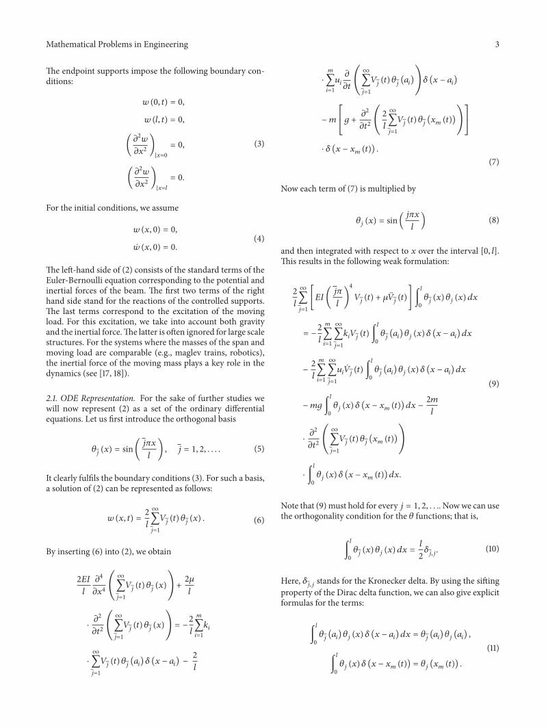
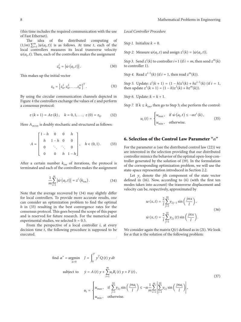
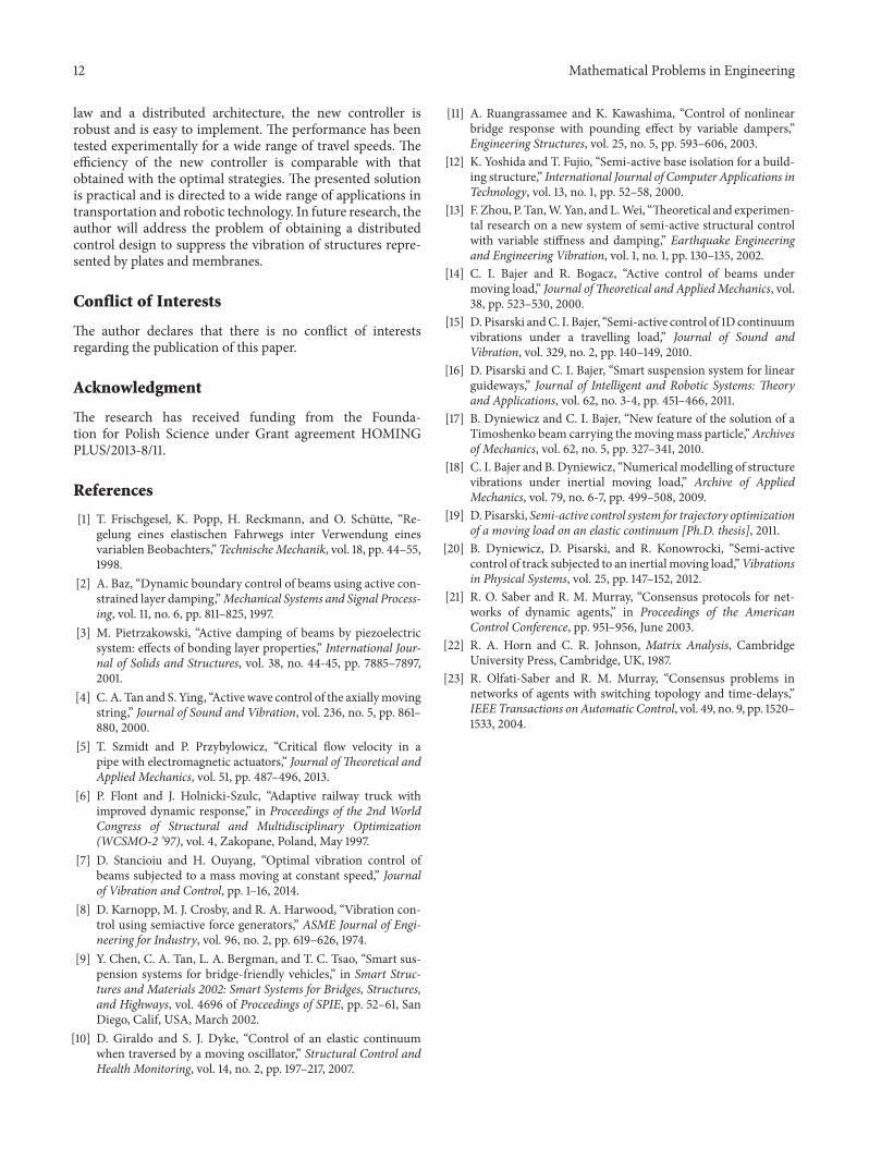in mechanical systems was proposed by Karnopp Crosbyand Harwood In [8] they presented the idea of stabilizingof the oscillator with one degree of freedom moving uponuneven ground The algorithm developed by the authorsldquoSkyhookrdquo is today one of the most widely used ones insuspension control systems for vehiclesThe idea was initiallydesigned to improve the comfort of passengers Later similarcontrol method was adopted to the oscillator moving uponcarrying structures Extensive results were demonstratedin [9 10] Controlled dampers are incorporated also forseismic isolation Interesting results can be found in [11 12]In [13] the authors proposed to control both the stiffnessand damping parameters The control decision led to themaximum dissipation of energy

The use of semiactive supports for a structure subjectedto a moving load was first proposed in [14] By means ofnumerical simulations the authors demonstrated that for awide range of travel velocities switching damping strategiesoutperform standard passive solutions The idea was laterextended in [15 16] where by introducing a rigorous analysisand optimization techniques the authors concluded that evenone switching action for each damper can provide verysmooth load passages A metric corresponding to the totaldeflection of the load trajectory from the desired straightline was reduced by up to 50 percent The drawbacks ofthe proposed method lie in its complicated implementationand high sensitivity to system uncertainties As the authorsdemonstrated in order to provide a desired performanceopen-loop switched solutions need to be recomputed everytime we expect a different travel speed

This paper proposes a novel control method to reduce thevibration levels of carrying structures subjected to movingloads The method is dedicated to the applications to largescale structures like bridges and overpasses subjected totraveling trains as well as to robotic guideways subjected toeffectors performing technological processes for examplecutting bonding or painting The control objective is toprovide a smooth passage of the traveling load and to extendthe safe life-time of the carrying structures The proposedcontrol strategy is based on the optimal centralized open-loop solutions presented in [15 16] but due to a distributedcontroller architecture and a state feedback control law it is alot more practical and robust

For the distributed controller we will impose the fol-lowing requirements functional symmetry in the controllerrsquosstructure theminimumcomputational burden and informa-tion exchange The symmetry will be achieved by splittingthe controller intomodules realizing the same computationalprocedures The modular type of architecture is convenientfor system assembly and maintenance Each of the moduleswill compute its control decision by using local state informa-tion and the average state of the whole structure The aver-age state will be reconstructed by exchanging informationbetween the neighboring controllers The final tuning of thecontroller was done by solving a corresponding optimizationproblem Then a series of experiments on a physical modelof a controlled guideway was performed As will be demon-strated the proposed controlmethod provides a performance

l

w

0

0 x

m


xm(t)

(t)

km

am

um

EI 120583

k1

a1

u1 k2

a2

u2

Figure 1 A span supported by set of controlled dampers andsubjected to a mass travelling at speed V(119905)

that is comparable with the optimal centralized solutions andit is robust to changes in the speed of the traveling load

The rest of this paper is structured as follows A math-ematical model of a carrying structure supported with a setof controlled dampers and subjected to a traveling load ispresented in Section 2 Section 3 introduces the distributedcontroller architecture and defines the local control lawsThe distributed averaging problem is studied in Section 4 InSection 5 an explicit procedure for the controller implemen-tation is given In Section 6 a method for finding an optimalparameter of the controller is presented Finally the resultsof experimental tests of the performance of the designedcontroller will be presented in Section 7

2 Investigated System

In this section we will introduce a mathematical represen-tation of a carrying structure supported by set of controlleddampers illustrated in Figure 1 This representation will beused in the final tuning of the proposed controller (seeSection 6)

For themodel of the span we will use the Euler-Bernoullibeam equation which is broadly applied to thin elastic bodiessubjected to small deflections A beam of the total length 119897is characterized by the bending stiffness 119864119868 and density perunit length 120583 A set of controlled supports are located at thepositions 119886

119894 For each of the supports we assume a controlled

damping 119906119894andor a fixed stiffness 119896

119894 The beam is subjected

to a mass 119898 travelling at the time-varying velocity V = V(119905)that is assumed to be given Position of the mass is denotedby 119909119898(119905) and computed by using

119909119898 (119905) = int

119905

0

V (119905) 119889119905 (1)

Denoting the transverse deflection of the span by 119908(119909 119905) thesystem is governed by

1198641198681205974119908 (119909 119905)

1205971199094+ 120583

1205972119908 (119909 119905)

1205971199052

= minus

119898

sum119894=1

(119896119894119908 (119886119894 119905) + 119906

119894

120597119908 (119886119894 119905)

120597119905) 120575 (119909 minus 119886

119894)

minus 119898(119892 +1205972119908 (119909119898 (119905) 119905)

1205971199052)120575 (119909 minus 119909

119898 (119905))

(2)



119908 (0 119905) = 0

119908 (119897 119905) = 0

(1205972119908

1205971199092)|119909=0

= 0

(1205972119908

1205971199092)|119909=119897

= 0

(3)


119908 (119909 0) = 0

(119909 0) = 0(4)



120579119895(119909) = sin(

119895120587119909

119897) 119895 = 1 2 (5)


119908 (119909 119905) =2

119897

infin

sum

119895=1

119881119895(119905) 120579119895(119909) (6)


2119864119868

119897

1205974

1205971199094(

infin

sum

119895=1

119881119895(119905) 120579119895(119909)) +

2120583

119897

sdot1205972

1205971199052(

infin

sum

119895=1

119881119895(119905) 120579119895(119909)) = minus

2

119897

119898

sum119894=1

119896119894

sdot

infin

sum

119895=1

119881119895(119905) 120579119895(119886119894) 120575 (119909 minus 119886

119894) minus

2

119897

sdot

119898

sum119894=1

119906119894

120597

120597119905(

infin

sum

119895=1

119881119895(119905) 120579119895(119886119894))120575 (119909 minus 119886

119894)

minus 119898[

[

119892 +1205972

1205971199052(2

119897

infin

sum

119895=1

119881119895(119905) 120579119895(119909119898 (119905)))

]

]

sdot 120575 (119909 minus 119909119898 (119905))

(7)


120579119895 (119909) = sin(

119895120587119909

119897) (8)


2

119897

infin

sum

119895=1

[119864119868(119895120587

119897)

4

119881119895(119905) + 120583

119895(119905)]int

119897

0

120579119895(119909) 120579119895 (119909) 119889119909

= minus2

119897

119898

sum119894=1

infin

sum

119895=1

119896119894119881119895(119905) int119897

0

120579119895(119886119894) 120579119895 (119909) 120575 (119909 minus 119886119894) 119889119909

minus2

119897

119898

sum119894=1

infin

sum

119895=1

119906119894119895(119905) int119897

0

120579119895(119886119894) 120579119895 (119909) 120575 (119909 minus 119886119894) 119889119909

minus 119898119892int119897

0

120579119895 (119909) 120575 (119909 minus 119909119898 (119905)) 119889119909 minus

2119898

119897

sdot1205972

1205971199052(

infin

sum

119895=1

119881119895(119905) 120579119895(119909119898 (119905)))

sdot int119897

0

120579119895 (119909) 120575 (119909 minus 119909119898 (119905)) 119889119909

(9)


int119897

0

120579119895(119909) 120579119895 (119909) 119889119909 =

119897

2120575119895119895 (10)

Here 120575119895119895


int119897

0

120579119895(119886119894) 120579119895 (119909) 120575 (119909 minus 119886119894) 119889119909 = 120579119895 (119886119894) 120579119895 (119886119894)

int119897

0

120579119895 (119909) 120575 (119909 minus 119909119898 (119905)) = 120579119895 (119909119898 (119905))

(11)



120583

infin

sum

119895=1

119895(119905) 120575119895119895+ 119864119868

infin

sum

119895=1

(119895120587

119897)

4

119881119895(119905) 120575119895119895

= minus2

119897

119898

sum119894=1

infin

sum

119895=1

(119896119894119881119895(119905) + 119906119894119895 (119905)) 120579119895 (119886119894) 120579119895 (119886119894)

minus 119898119892120579119895(119909119898 (119905))

minus2119898

119897

1205972

1205971199052(

infin

sum

119895=1

119881119895(119905) 120579119895(119909119898 (119905))) 120579119895 (119909119898 (119905))

119895 = 1 2

(12)



given below

1205972

1205971199052(

infin

sum

119895=1

119881119895(119905) 120579119895(119909119898 (119905)))

=

infin

sum

119895=1

119895(119905) 120579119895(119909119898 (119905))

+

infin

sum

119895=1

2119895120587

119897119895(119905) 120601119895(119909119898 (119905)) V (119905)

+

infin

sum

119895=1

119895120587

119897119881119895(119905) 120601119895(119909119898 (119905)) V (119905)

minus

infin

sum

119895=1

1198952

1205872

1198972119881119895(119905) 120579119895(119909119898 (119905)) (V (119905))

2

(13)


119898(119905)119897)


119908 (119909 119905) =2

119897

infin

sum

119895=1

119881119895(119905) 120579119895(119909)

120583119895 (119905) + 119864119868 (

119895120587

119897)4

119881119895 (119905)

= minus2

119897

119898

sum119894=1

infin

sum

119895=1

(119896119894119881119895(119905) + 119906119894119895 (119905)) 120579119895 (119886119894) 120579119895 (119886119894)

minus 119898119892120579119895(119909119898 (119905))

minus2119898

119897

infin

sum

119895=1

119895(119905) 120579119895(119909119898 (119905)) 120579119895 (119909119898 (119905))

minus4119898

119897

infin

sum

119895=1

119895120587

119897119895(119905) 120601119895(119909119898 (119905)) 120579119895 (119909119898 (119905)) V (119905)

minus2119898

119897

infin

sum

119895=1

119895120587

119897119881119895(119905) 120601119895(119909119898 (119905)) 120579119895 (119909119898 (119905)) V (119905)

+2119898

119897

infin

sum

119895=1

1198952

1205872

1198972119881119895(119905) 120579119895(119909119898 (119905)) 120579119895 (119909119898 (119905)) (V (119905))

2

119895 = 1 2

(14)


119881119895 (0) = 0

119895 (0) = 0

119895 = 1 2

(15)


119895(119905) and




119910 (119905)

= [1198811 (119905) 1 (119905) 1198812 (119905) 2 (119905) 119881119899 (119905) 119899 (119905)]

119879

(16)


119910 = 119860 (119905) 119910 +

119898

sum119894=1

119906119894119861119894 (119905) 119910 + 119865 (119905)

119910 (0) = 0

(17)



+ (18)

3 Control Design





um

w1 w2 w3 wm


u3u2u1





Centralcomputer


u1u2

u3um

w1w2

w3

wm



119894 119905) (119886





Local

u1 u2 u3 umw1w1 w2

w2 w3w3

wm

wm

wmminus1

computerLocal

computerLocal

computerLocal

computer








119869 = int119879

0

119910119879119876 (119905) 119910 119889119905

under 119910 = 119860 (119905) 119910 +

119898

sum119894=1

119906119894119861119894 (119905) 119910 + 119865 (119905)

(19)


119897 = int119879

0

V (119905) 119889119905 (20)


119910119879119876 (119905) 119910 = (119908 (V119905 119905))2 (21)




u1(t)

u2(t)

u3(t)

um(t)

0 1205911 1205912 1205913 120591m tf t

umaxumin








1 that is (119886






1returns toward the







119906119894 (119905) =

119906max if (119886119894 119905) le minus120572

1

119898

119898

sum119894=1

1003816100381610038161003816 (119886119894 119905)1003816100381610038161003816






119911 (119896 + 1) = 119860119911 (119896) 119896 = 0 1

119911 (0) = 1199110 119911 isin R119899

(23)





ttf1205911ttf1205911

w(a1 t) (1m)sum m

i=1| (ai t)|

12

12

w


(1119898)sum119898



1



lowast satisfying

119911lowast= 1198881 (24)


1198601 = 1 (25)



1198601198791 = 1 (26)


lim119896rarrinfin

119860119896=1

11989911119879 (27)

10 15 20 25 305k

020406080

100

z(k)




119894=1119911119894 (0)

1198991 (28)


119911 (119896 + 1) =

[[[[[

[

05 0 0 05

05 05 0 0

0 05 05 0

0 0 05 05

]]]]]

]

119911 (119896) (29)







119898



119911119894

0=1003816100381610038161003816 (119886119894 119905)

1003816100381610038161003816 (30)


1199110= [1199111

0 1199112

0 119911

119898

0]119879

(31)


119911 (119896 + 1) = 119860119911 (119896) 119896 = 0 1 119911 (0) = 1199110 (32)

Here 119860119898times119898


119860 =

[[[[[

[

1 minus ℎ 0 0 ℎ

ℎ 1 minus ℎ 0 0

0 d d 0

0 0 ℎ 1 minus ℎ

]]]]]

]

ℎ isin (0 1) (33)



1

119898

119898

sum119894=1

1003816100381610038161003816 (119886119894 119905)1003816100381610038161003816 = 119911119894(119896119905119898) (34)






119894 119905)|




Step 6 Update 119896 = 119896 + 1


119906119894 (119905) =

119906max if (119886119894 119905) le minus120572119911119894 (119896)






119908 (119909 119905) =2

119897

10

sum119895=1

1199102119895minus1

sin(119895120587119909

119897)

(119909 119905) =2

119897

10

sum119895=1

1199102119895 (119905) sin(

119895120587119909

119897)

(36)



119869 = int119879

0

119910119879119876 (119905) 119910 119889119905

subject to 119910 = 119860 (119905) 119910 +

119898

sum119894=1

119906119894119861119894 (119905) 119910 + 119865 (119905)

119906119894=

119906max if10

sum119895=1

1199102119895sin(

119895120587119886119894

119897) le minus120572

1

119898

119898

sum119894=1

10038161003816100381610038161003816100381610038161003816100381610038161003816

10

sum119895=1

1199102119895sin(

119895120587119886119894

119897)

10038161003816100381610038161003816100381610038161003816100381610038161003816

119906min otherwise

(37)


(a) (b)







1= 15119897 119886

2= 25119897

1198863= 35119897 and 119886





1 1198962) 1000Nm










1198691= int119897

0

int119879

0

(119908 (119909 119905))2119889119909 119889119905

1198692= max119909isin[0119897]119905isin[0119879]

|119908 (119909 119905)|

1198693= int119879

0

(119908 (V119905 119905))2 119889119905

1198694= max119905isin[0119879]

|119908 (V119905 119905)|

(38)



4correspond to





0

1

0

1

xl ttf


05

w(xt)

(mm

)




05

w(tt)

(mm

)

01 02 03 04 05 06 07 08 09 10ttf






01 02 03 04 05 06 07 08 09 10ttf

01 02 03 04 05 06 07 08 09 10ttf

01 02 03 04 05 06 07 08 09 10ttf

01 02 03 04 05 06 07 08 09 10ttf

umin

umax

u1(t)

umin

umax

u2(t)

umin

umax

u3(t)

umin

umax

u4(t)


01 02 03 04 05 06 07 08 09 10ttf

01 02 03 04 05 06 07 08 09 10ttf

01 02 03 04 05 06 07 08 09 10ttf

01 02 03 04 05 06 07 08 09 10ttf

umin

umax

u1(t)

umin

umax

u2(t)

umin

umax

u3(t)

umin

umax

u4(t)




1 1000 0460 0501

2 1000 0351 0389

4 1000 0228 0265








01 02 03 04 05 06 07 08 09 10ttf

minus25

minus20

minus15

minus10

minus5

05

w(tt)

(mm

)




1 1000 0808 0812

2 1000 0734 0778

4 1000 0642 0691



1 1000 0539 0594

2 1000 0388 0407

4 1000 0319 0342



1 1000 0812 0837

2 1000 0719 0755

4 1000 0658 0714


8 Conclusion






Acknowledgment


References































Volume 2014




Journal of











Journal of


Function Spaces






Algebra











119908 (0 119905) = 0

119908 (119897 119905) = 0

(1205972119908

1205971199092)|119909=0

= 0

(1205972119908

1205971199092)|119909=119897

= 0

(3)


119908 (119909 0) = 0

(119909 0) = 0(4)



120579119895(119909) = sin(

119895120587119909

119897) 119895 = 1 2 (5)


119908 (119909 119905) =2

119897

infin

sum

119895=1

119881119895(119905) 120579119895(119909) (6)


2119864119868

119897

1205974

1205971199094(

infin

sum

119895=1

119881119895(119905) 120579119895(119909)) +

2120583

119897

sdot1205972

1205971199052(

infin

sum

119895=1

119881119895(119905) 120579119895(119909)) = minus

2

119897

119898

sum119894=1

119896119894

sdot

infin

sum

119895=1

119881119895(119905) 120579119895(119886119894) 120575 (119909 minus 119886

119894) minus

2

119897

sdot

119898

sum119894=1

119906119894

120597

120597119905(

infin

sum

119895=1

119881119895(119905) 120579119895(119886119894))120575 (119909 minus 119886

119894)

minus 119898[

[

119892 +1205972

1205971199052(2

119897

infin

sum

119895=1

119881119895(119905) 120579119895(119909119898 (119905)))

]

]

sdot 120575 (119909 minus 119909119898 (119905))

(7)


120579119895 (119909) = sin(

119895120587119909

119897) (8)


2

119897

infin

sum

119895=1

[119864119868(119895120587

119897)

4

119881119895(119905) + 120583

119895(119905)]int

119897

0

120579119895(119909) 120579119895 (119909) 119889119909

= minus2

119897

119898

sum119894=1

infin

sum

119895=1

119896119894119881119895(119905) int119897

0

120579119895(119886119894) 120579119895 (119909) 120575 (119909 minus 119886119894) 119889119909

minus2

119897

119898

sum119894=1

infin

sum

119895=1

119906119894119895(119905) int119897

0

120579119895(119886119894) 120579119895 (119909) 120575 (119909 minus 119886119894) 119889119909

minus 119898119892int119897

0

120579119895 (119909) 120575 (119909 minus 119909119898 (119905)) 119889119909 minus

2119898

119897

sdot1205972

1205971199052(

infin

sum

119895=1

119881119895(119905) 120579119895(119909119898 (119905)))

sdot int119897

0

120579119895 (119909) 120575 (119909 minus 119909119898 (119905)) 119889119909

(9)


int119897

0

120579119895(119909) 120579119895 (119909) 119889119909 =

119897

2120575119895119895 (10)

Here 120575119895119895


int119897

0

120579119895(119886119894) 120579119895 (119909) 120575 (119909 minus 119886119894) 119889119909 = 120579119895 (119886119894) 120579119895 (119886119894)

int119897

0

120579119895 (119909) 120575 (119909 minus 119909119898 (119905)) = 120579119895 (119909119898 (119905))

(11)



120583

infin

sum

119895=1

119895(119905) 120575119895119895+ 119864119868

infin

sum

119895=1

(119895120587

119897)

4

119881119895(119905) 120575119895119895

= minus2

119897

119898

sum119894=1

infin

sum

119895=1

(119896119894119881119895(119905) + 119906119894119895 (119905)) 120579119895 (119886119894) 120579119895 (119886119894)

minus 119898119892120579119895(119909119898 (119905))

minus2119898

119897

1205972

1205971199052(

infin

sum

119895=1

119881119895(119905) 120579119895(119909119898 (119905))) 120579119895 (119909119898 (119905))

119895 = 1 2

(12)



given below

1205972

1205971199052(

infin

sum

119895=1

119881119895(119905) 120579119895(119909119898 (119905)))

=

infin

sum

119895=1

119895(119905) 120579119895(119909119898 (119905))

+

infin

sum

119895=1

2119895120587

119897119895(119905) 120601119895(119909119898 (119905)) V (119905)

+

infin

sum

119895=1

119895120587

119897119881119895(119905) 120601119895(119909119898 (119905)) V (119905)

minus

infin

sum

119895=1

1198952

1205872

1198972119881119895(119905) 120579119895(119909119898 (119905)) (V (119905))

2

(13)


119898(119905)119897)


119908 (119909 119905) =2

119897

infin

sum

119895=1

119881119895(119905) 120579119895(119909)

120583119895 (119905) + 119864119868 (

119895120587

119897)4

119881119895 (119905)

= minus2

119897

119898

sum119894=1

infin

sum

119895=1

(119896119894119881119895(119905) + 119906119894119895 (119905)) 120579119895 (119886119894) 120579119895 (119886119894)

minus 119898119892120579119895(119909119898 (119905))

minus2119898

119897

infin

sum

119895=1

119895(119905) 120579119895(119909119898 (119905)) 120579119895 (119909119898 (119905))

minus4119898

119897

infin

sum

119895=1

119895120587

119897119895(119905) 120601119895(119909119898 (119905)) 120579119895 (119909119898 (119905)) V (119905)

minus2119898

119897

infin

sum

119895=1

119895120587

119897119881119895(119905) 120601119895(119909119898 (119905)) 120579119895 (119909119898 (119905)) V (119905)

+2119898

119897

infin

sum

119895=1

1198952

1205872

1198972119881119895(119905) 120579119895(119909119898 (119905)) 120579119895 (119909119898 (119905)) (V (119905))

2

119895 = 1 2

(14)


119881119895 (0) = 0

119895 (0) = 0

119895 = 1 2

(15)


119895(119905) and




119910 (119905)

= [1198811 (119905) 1 (119905) 1198812 (119905) 2 (119905) 119881119899 (119905) 119899 (119905)]

119879

(16)


119910 = 119860 (119905) 119910 +

119898

sum119894=1

119906119894119861119894 (119905) 119910 + 119865 (119905)

119910 (0) = 0

(17)



+ (18)

3 Control Design





um

w1 w2 w3 wm


u3u2u1





Centralcomputer


u1u2

u3um

w1w2

w3

wm



119894 119905) (119886





Local

u1 u2 u3 umw1w1 w2

w2 w3w3

wm

wm

wmminus1

computerLocal

computerLocal

computerLocal

computer








119869 = int119879

0

119910119879119876 (119905) 119910 119889119905

under 119910 = 119860 (119905) 119910 +

119898

sum119894=1

119906119894119861119894 (119905) 119910 + 119865 (119905)

(19)


119897 = int119879

0

V (119905) 119889119905 (20)


119910119879119876 (119905) 119910 = (119908 (V119905 119905))2 (21)




u1(t)

u2(t)

u3(t)

um(t)

0 1205911 1205912 1205913 120591m tf t

umaxumin








1 that is (119886






1returns toward the







119906119894 (119905) =

119906max if (119886119894 119905) le minus120572

1

119898

119898

sum119894=1

1003816100381610038161003816 (119886119894 119905)1003816100381610038161003816






119911 (119896 + 1) = 119860119911 (119896) 119896 = 0 1

119911 (0) = 1199110 119911 isin R119899

(23)





ttf1205911ttf1205911

w(a1 t) (1m)sum m

i=1| (ai t)|

12

12

w


(1119898)sum119898



1



lowast satisfying

119911lowast= 1198881 (24)


1198601 = 1 (25)



1198601198791 = 1 (26)


lim119896rarrinfin

119860119896=1

11989911119879 (27)

10 15 20 25 305k

020406080

100

z(k)




119894=1119911119894 (0)

1198991 (28)


119911 (119896 + 1) =

[[[[[

[

05 0 0 05

05 05 0 0

0 05 05 0

0 0 05 05

]]]]]

]

119911 (119896) (29)







119898



119911119894

0=1003816100381610038161003816 (119886119894 119905)

1003816100381610038161003816 (30)


1199110= [1199111

0 1199112

0 119911

119898

0]119879

(31)


119911 (119896 + 1) = 119860119911 (119896) 119896 = 0 1 119911 (0) = 1199110 (32)

Here 119860119898times119898


119860 =

[[[[[

[

1 minus ℎ 0 0 ℎ

ℎ 1 minus ℎ 0 0

0 d d 0

0 0 ℎ 1 minus ℎ

]]]]]

]

ℎ isin (0 1) (33)



1

119898

119898

sum119894=1

1003816100381610038161003816 (119886119894 119905)1003816100381610038161003816 = 119911119894(119896119905119898) (34)






119894 119905)|




Step 6 Update 119896 = 119896 + 1


119906119894 (119905) =

119906max if (119886119894 119905) le minus120572119911119894 (119896)






119908 (119909 119905) =2

119897

10

sum119895=1

1199102119895minus1

sin(119895120587119909

119897)

(119909 119905) =2

119897

10

sum119895=1

1199102119895 (119905) sin(

119895120587119909

119897)

(36)



119869 = int119879

0

119910119879119876 (119905) 119910 119889119905

subject to 119910 = 119860 (119905) 119910 +

119898

sum119894=1

119906119894119861119894 (119905) 119910 + 119865 (119905)

119906119894=

119906max if10

sum119895=1

1199102119895sin(

119895120587119886119894

119897) le minus120572

1

119898

119898

sum119894=1

10038161003816100381610038161003816100381610038161003816100381610038161003816

10

sum119895=1

1199102119895sin(

119895120587119886119894

119897)

10038161003816100381610038161003816100381610038161003816100381610038161003816

119906min otherwise

(37)


(a) (b)







1= 15119897 119886

2= 25119897

1198863= 35119897 and 119886





1 1198962) 1000Nm










1198691= int119897

0

int119879

0

(119908 (119909 119905))2119889119909 119889119905

1198692= max119909isin[0119897]119905isin[0119879]

|119908 (119909 119905)|

1198693= int119879

0

(119908 (V119905 119905))2 119889119905

1198694= max119905isin[0119879]

|119908 (V119905 119905)|

(38)



4correspond to





0

1

0

1

xl ttf


05

w(xt)

(mm

)




05

w(tt)

(mm

)

01 02 03 04 05 06 07 08 09 10ttf






01 02 03 04 05 06 07 08 09 10ttf

01 02 03 04 05 06 07 08 09 10ttf

01 02 03 04 05 06 07 08 09 10ttf

01 02 03 04 05 06 07 08 09 10ttf

umin

umax

u1(t)

umin

umax

u2(t)

umin

umax

u3(t)

umin

umax

u4(t)


01 02 03 04 05 06 07 08 09 10ttf

01 02 03 04 05 06 07 08 09 10ttf

01 02 03 04 05 06 07 08 09 10ttf

01 02 03 04 05 06 07 08 09 10ttf

umin

umax

u1(t)

umin

umax

u2(t)

umin

umax

u3(t)

umin

umax

u4(t)




1 1000 0460 0501

2 1000 0351 0389

4 1000 0228 0265








01 02 03 04 05 06 07 08 09 10ttf

minus25

minus20

minus15

minus10

minus5

05

w(tt)

(mm

)




1 1000 0808 0812

2 1000 0734 0778

4 1000 0642 0691



1 1000 0539 0594

2 1000 0388 0407

4 1000 0319 0342



1 1000 0812 0837

2 1000 0719 0755

4 1000 0658 0714


8 Conclusion






Acknowledgment


References































Volume 2014




Journal of











Journal of


Function Spaces






Algebra











120583

infin

sum

119895=1

119895(119905) 120575119895119895+ 119864119868

infin

sum

119895=1

(119895120587

119897)

4

119881119895(119905) 120575119895119895

= minus2

119897

119898

sum119894=1

infin

sum

119895=1

(119896119894119881119895(119905) + 119906119894119895 (119905)) 120579119895 (119886119894) 120579119895 (119886119894)

minus 119898119892120579119895(119909119898 (119905))

minus2119898

119897

1205972

1205971199052(

infin

sum

119895=1

119881119895(119905) 120579119895(119909119898 (119905))) 120579119895 (119909119898 (119905))

119895 = 1 2

(12)



given below

1205972

1205971199052(

infin

sum

119895=1

119881119895(119905) 120579119895(119909119898 (119905)))

=

infin

sum

119895=1

119895(119905) 120579119895(119909119898 (119905))

+

infin

sum

119895=1

2119895120587

119897119895(119905) 120601119895(119909119898 (119905)) V (119905)

+

infin

sum

119895=1

119895120587

119897119881119895(119905) 120601119895(119909119898 (119905)) V (119905)

minus

infin

sum

119895=1

1198952

1205872

1198972119881119895(119905) 120579119895(119909119898 (119905)) (V (119905))

2

(13)


119898(119905)119897)


119908 (119909 119905) =2

119897

infin

sum

119895=1

119881119895(119905) 120579119895(119909)

120583119895 (119905) + 119864119868 (

119895120587

119897)4

119881119895 (119905)

= minus2

119897

119898

sum119894=1

infin

sum

119895=1

(119896119894119881119895(119905) + 119906119894119895 (119905)) 120579119895 (119886119894) 120579119895 (119886119894)

minus 119898119892120579119895(119909119898 (119905))

minus2119898

119897

infin

sum

119895=1

119895(119905) 120579119895(119909119898 (119905)) 120579119895 (119909119898 (119905))

minus4119898

119897

infin

sum

119895=1

119895120587

119897119895(119905) 120601119895(119909119898 (119905)) 120579119895 (119909119898 (119905)) V (119905)

minus2119898

119897

infin

sum

119895=1

119895120587

119897119881119895(119905) 120601119895(119909119898 (119905)) 120579119895 (119909119898 (119905)) V (119905)

+2119898

119897

infin

sum

119895=1

1198952

1205872

1198972119881119895(119905) 120579119895(119909119898 (119905)) 120579119895 (119909119898 (119905)) (V (119905))

2

119895 = 1 2

(14)


119881119895 (0) = 0

119895 (0) = 0

119895 = 1 2

(15)


119895(119905) and




119910 (119905)

= [1198811 (119905) 1 (119905) 1198812 (119905) 2 (119905) 119881119899 (119905) 119899 (119905)]

119879

(16)


119910 = 119860 (119905) 119910 +

119898

sum119894=1

119906119894119861119894 (119905) 119910 + 119865 (119905)

119910 (0) = 0

(17)



+ (18)

3 Control Design





um

w1 w2 w3 wm


u3u2u1





Centralcomputer


u1u2

u3um

w1w2

w3

wm



119894 119905) (119886





Local

u1 u2 u3 umw1w1 w2

w2 w3w3

wm

wm

wmminus1

computerLocal

computerLocal

computerLocal

computer








119869 = int119879

0

119910119879119876 (119905) 119910 119889119905

under 119910 = 119860 (119905) 119910 +

119898

sum119894=1

119906119894119861119894 (119905) 119910 + 119865 (119905)

(19)


119897 = int119879

0

V (119905) 119889119905 (20)


119910119879119876 (119905) 119910 = (119908 (V119905 119905))2 (21)




u1(t)

u2(t)

u3(t)

um(t)

0 1205911 1205912 1205913 120591m tf t

umaxumin








1 that is (119886






1returns toward the







119906119894 (119905) =

119906max if (119886119894 119905) le minus120572

1

119898

119898

sum119894=1

1003816100381610038161003816 (119886119894 119905)1003816100381610038161003816






119911 (119896 + 1) = 119860119911 (119896) 119896 = 0 1

119911 (0) = 1199110 119911 isin R119899

(23)





ttf1205911ttf1205911

w(a1 t) (1m)sum m

i=1| (ai t)|

12

12

w


(1119898)sum119898



1



lowast satisfying

119911lowast= 1198881 (24)


1198601 = 1 (25)



1198601198791 = 1 (26)


lim119896rarrinfin

119860119896=1

11989911119879 (27)

10 15 20 25 305k

020406080

100

z(k)




119894=1119911119894 (0)

1198991 (28)


119911 (119896 + 1) =

[[[[[

[

05 0 0 05

05 05 0 0

0 05 05 0

0 0 05 05

]]]]]

]

119911 (119896) (29)







119898



119911119894

0=1003816100381610038161003816 (119886119894 119905)

1003816100381610038161003816 (30)


1199110= [1199111

0 1199112

0 119911

119898

0]119879

(31)


119911 (119896 + 1) = 119860119911 (119896) 119896 = 0 1 119911 (0) = 1199110 (32)

Here 119860119898times119898


119860 =

[[[[[

[

1 minus ℎ 0 0 ℎ

ℎ 1 minus ℎ 0 0

0 d d 0

0 0 ℎ 1 minus ℎ

]]]]]

]

ℎ isin (0 1) (33)



1

119898

119898

sum119894=1

1003816100381610038161003816 (119886119894 119905)1003816100381610038161003816 = 119911119894(119896119905119898) (34)






119894 119905)|




Step 6 Update 119896 = 119896 + 1


119906119894 (119905) =

119906max if (119886119894 119905) le minus120572119911119894 (119896)






119908 (119909 119905) =2

119897

10

sum119895=1

1199102119895minus1

sin(119895120587119909

119897)

(119909 119905) =2

119897

10

sum119895=1

1199102119895 (119905) sin(

119895120587119909

119897)

(36)



119869 = int119879

0

119910119879119876 (119905) 119910 119889119905

subject to 119910 = 119860 (119905) 119910 +

119898

sum119894=1

119906119894119861119894 (119905) 119910 + 119865 (119905)

119906119894=

119906max if10

sum119895=1

1199102119895sin(

119895120587119886119894

119897) le minus120572

1

119898

119898

sum119894=1

10038161003816100381610038161003816100381610038161003816100381610038161003816

10

sum119895=1

1199102119895sin(

119895120587119886119894

119897)

10038161003816100381610038161003816100381610038161003816100381610038161003816

119906min otherwise

(37)


(a) (b)







1= 15119897 119886

2= 25119897

1198863= 35119897 and 119886





1 1198962) 1000Nm










1198691= int119897

0

int119879

0

(119908 (119909 119905))2119889119909 119889119905

1198692= max119909isin[0119897]119905isin[0119879]

|119908 (119909 119905)|

1198693= int119879

0

(119908 (V119905 119905))2 119889119905

1198694= max119905isin[0119879]

|119908 (V119905 119905)|

(38)



4correspond to





0

1

0

1

xl ttf


05

w(xt)

(mm

)




05

w(tt)

(mm

)

01 02 03 04 05 06 07 08 09 10ttf






01 02 03 04 05 06 07 08 09 10ttf

01 02 03 04 05 06 07 08 09 10ttf

01 02 03 04 05 06 07 08 09 10ttf

01 02 03 04 05 06 07 08 09 10ttf

umin

umax

u1(t)

umin

umax

u2(t)

umin

umax

u3(t)

umin

umax

u4(t)


01 02 03 04 05 06 07 08 09 10ttf

01 02 03 04 05 06 07 08 09 10ttf

01 02 03 04 05 06 07 08 09 10ttf

01 02 03 04 05 06 07 08 09 10ttf

umin

umax

u1(t)

umin

umax

u2(t)

umin

umax

u3(t)

umin

umax

u4(t)




1 1000 0460 0501

2 1000 0351 0389

4 1000 0228 0265








01 02 03 04 05 06 07 08 09 10ttf

minus25

minus20

minus15

minus10

minus5

05

w(tt)

(mm

)




1 1000 0808 0812

2 1000 0734 0778

4 1000 0642 0691



1 1000 0539 0594

2 1000 0388 0407

4 1000 0319 0342



1 1000 0812 0837

2 1000 0719 0755

4 1000 0658 0714


8 Conclusion






Acknowledgment


References































Volume 2014




Journal of











Journal of


Function Spaces






Algebra










um

w1 w2 w3 wm


u3u2u1





Centralcomputer


u1u2

u3um

w1w2

w3

wm



119894 119905) (119886





Local

u1 u2 u3 umw1w1 w2

w2 w3w3

wm

wm

wmminus1

computerLocal

computerLocal

computerLocal

computer








119869 = int119879

0

119910119879119876 (119905) 119910 119889119905

under 119910 = 119860 (119905) 119910 +

119898

sum119894=1

119906119894119861119894 (119905) 119910 + 119865 (119905)

(19)


119897 = int119879

0

V (119905) 119889119905 (20)


119910119879119876 (119905) 119910 = (119908 (V119905 119905))2 (21)




u1(t)

u2(t)

u3(t)

um(t)

0 1205911 1205912 1205913 120591m tf t

umaxumin








1 that is (119886






1returns toward the







119906119894 (119905) =

119906max if (119886119894 119905) le minus120572

1

119898

119898

sum119894=1

1003816100381610038161003816 (119886119894 119905)1003816100381610038161003816






119911 (119896 + 1) = 119860119911 (119896) 119896 = 0 1

119911 (0) = 1199110 119911 isin R119899

(23)





ttf1205911ttf1205911

w(a1 t) (1m)sum m

i=1| (ai t)|

12

12

w


(1119898)sum119898



1



lowast satisfying

119911lowast= 1198881 (24)


1198601 = 1 (25)



1198601198791 = 1 (26)


lim119896rarrinfin

119860119896=1

11989911119879 (27)

10 15 20 25 305k

020406080

100

z(k)




119894=1119911119894 (0)

1198991 (28)


119911 (119896 + 1) =

[[[[[

[

05 0 0 05

05 05 0 0

0 05 05 0

0 0 05 05

]]]]]

]

119911 (119896) (29)







119898



119911119894

0=1003816100381610038161003816 (119886119894 119905)

1003816100381610038161003816 (30)


1199110= [1199111

0 1199112

0 119911

119898

0]119879

(31)


119911 (119896 + 1) = 119860119911 (119896) 119896 = 0 1 119911 (0) = 1199110 (32)

Here 119860119898times119898


119860 =

[[[[[

[

1 minus ℎ 0 0 ℎ

ℎ 1 minus ℎ 0 0

0 d d 0

0 0 ℎ 1 minus ℎ

]]]]]

]

ℎ isin (0 1) (33)



1

119898

119898

sum119894=1

1003816100381610038161003816 (119886119894 119905)1003816100381610038161003816 = 119911119894(119896119905119898) (34)






119894 119905)|




Step 6 Update 119896 = 119896 + 1


119906119894 (119905) =

119906max if (119886119894 119905) le minus120572119911119894 (119896)






119908 (119909 119905) =2

119897

10

sum119895=1

1199102119895minus1

sin(119895120587119909

119897)

(119909 119905) =2

119897

10

sum119895=1

1199102119895 (119905) sin(

119895120587119909

119897)

(36)



119869 = int119879

0

119910119879119876 (119905) 119910 119889119905

subject to 119910 = 119860 (119905) 119910 +

119898

sum119894=1

119906119894119861119894 (119905) 119910 + 119865 (119905)

119906119894=

119906max if10

sum119895=1

1199102119895sin(

119895120587119886119894

119897) le minus120572

1

119898

119898

sum119894=1

10038161003816100381610038161003816100381610038161003816100381610038161003816

10

sum119895=1

1199102119895sin(

119895120587119886119894

119897)

10038161003816100381610038161003816100381610038161003816100381610038161003816

119906min otherwise

(37)


(a) (b)







1= 15119897 119886

2= 25119897

1198863= 35119897 and 119886





1 1198962) 1000Nm










1198691= int119897

0

int119879

0

(119908 (119909 119905))2119889119909 119889119905

1198692= max119909isin[0119897]119905isin[0119879]

|119908 (119909 119905)|

1198693= int119879

0

(119908 (V119905 119905))2 119889119905

1198694= max119905isin[0119879]

|119908 (V119905 119905)|

(38)



4correspond to





0

1

0

1

xl ttf


05

w(xt)

(mm

)




05

w(tt)

(mm

)

01 02 03 04 05 06 07 08 09 10ttf






01 02 03 04 05 06 07 08 09 10ttf

01 02 03 04 05 06 07 08 09 10ttf

01 02 03 04 05 06 07 08 09 10ttf

01 02 03 04 05 06 07 08 09 10ttf

umin

umax

u1(t)

umin

umax

u2(t)

umin

umax

u3(t)

umin

umax

u4(t)


01 02 03 04 05 06 07 08 09 10ttf

01 02 03 04 05 06 07 08 09 10ttf

01 02 03 04 05 06 07 08 09 10ttf

01 02 03 04 05 06 07 08 09 10ttf

umin

umax

u1(t)

umin

umax

u2(t)

umin

umax

u3(t)

umin

umax

u4(t)




1 1000 0460 0501

2 1000 0351 0389

4 1000 0228 0265








01 02 03 04 05 06 07 08 09 10ttf

minus25

minus20

minus15

minus10

minus5

05

w(tt)

(mm

)




1 1000 0808 0812

2 1000 0734 0778

4 1000 0642 0691



1 1000 0539 0594

2 1000 0388 0407

4 1000 0319 0342



1 1000 0812 0837

2 1000 0719 0755

4 1000 0658 0714


8 Conclusion






Acknowledgment


References































Volume 2014




Journal of











Journal of


Function Spaces






Algebra












u1(t)

u2(t)

u3(t)

um(t)

0 1205911 1205912 1205913 120591m tf t

umaxumin








1 that is (119886






1returns toward the







119906119894 (119905) =

119906max if (119886119894 119905) le minus120572

1

119898

119898

sum119894=1

1003816100381610038161003816 (119886119894 119905)1003816100381610038161003816






119911 (119896 + 1) = 119860119911 (119896) 119896 = 0 1

119911 (0) = 1199110 119911 isin R119899

(23)





ttf1205911ttf1205911

w(a1 t) (1m)sum m

i=1| (ai t)|

12

12

w


(1119898)sum119898



1



lowast satisfying

119911lowast= 1198881 (24)


1198601 = 1 (25)



1198601198791 = 1 (26)


lim119896rarrinfin

119860119896=1

11989911119879 (27)

10 15 20 25 305k

020406080

100

z(k)




119894=1119911119894 (0)

1198991 (28)


119911 (119896 + 1) =

[[[[[

[

05 0 0 05

05 05 0 0

0 05 05 0

0 0 05 05

]]]]]

]

119911 (119896) (29)







119898



119911119894

0=1003816100381610038161003816 (119886119894 119905)

1003816100381610038161003816 (30)


1199110= [1199111

0 1199112

0 119911

119898

0]119879

(31)


119911 (119896 + 1) = 119860119911 (119896) 119896 = 0 1 119911 (0) = 1199110 (32)

Here 119860119898times119898


119860 =

[[[[[

[

1 minus ℎ 0 0 ℎ

ℎ 1 minus ℎ 0 0

0 d d 0

0 0 ℎ 1 minus ℎ

]]]]]

]

ℎ isin (0 1) (33)



1

119898

119898

sum119894=1

1003816100381610038161003816 (119886119894 119905)1003816100381610038161003816 = 119911119894(119896119905119898) (34)






119894 119905)|




Step 6 Update 119896 = 119896 + 1


119906119894 (119905) =

119906max if (119886119894 119905) le minus120572119911119894 (119896)






119908 (119909 119905) =2

119897

10

sum119895=1

1199102119895minus1

sin(119895120587119909

119897)

(119909 119905) =2

119897

10

sum119895=1

1199102119895 (119905) sin(

119895120587119909

119897)

(36)



119869 = int119879

0

119910119879119876 (119905) 119910 119889119905

subject to 119910 = 119860 (119905) 119910 +

119898

sum119894=1

119906119894119861119894 (119905) 119910 + 119865 (119905)

119906119894=

119906max if10

sum119895=1

1199102119895sin(

119895120587119886119894

119897) le minus120572

1

119898

119898

sum119894=1

10038161003816100381610038161003816100381610038161003816100381610038161003816

10

sum119895=1

1199102119895sin(

119895120587119886119894

119897)

10038161003816100381610038161003816100381610038161003816100381610038161003816

119906min otherwise

(37)


(a) (b)







1= 15119897 119886

2= 25119897

1198863= 35119897 and 119886





1 1198962) 1000Nm










1198691= int119897

0

int119879

0

(119908 (119909 119905))2119889119909 119889119905

1198692= max119909isin[0119897]119905isin[0119879]

|119908 (119909 119905)|

1198693= int119879

0

(119908 (V119905 119905))2 119889119905

1198694= max119905isin[0119879]

|119908 (V119905 119905)|

(38)



4correspond to





0

1

0

1

xl ttf


05

w(xt)

(mm

)




05

w(tt)

(mm

)

01 02 03 04 05 06 07 08 09 10ttf






01 02 03 04 05 06 07 08 09 10ttf

01 02 03 04 05 06 07 08 09 10ttf

01 02 03 04 05 06 07 08 09 10ttf

01 02 03 04 05 06 07 08 09 10ttf

umin

umax

u1(t)

umin

umax

u2(t)

umin

umax

u3(t)

umin

umax

u4(t)


01 02 03 04 05 06 07 08 09 10ttf

01 02 03 04 05 06 07 08 09 10ttf

01 02 03 04 05 06 07 08 09 10ttf

01 02 03 04 05 06 07 08 09 10ttf

umin

umax

u1(t)

umin

umax

u2(t)

umin

umax

u3(t)

umin

umax

u4(t)




1 1000 0460 0501

2 1000 0351 0389

4 1000 0228 0265








01 02 03 04 05 06 07 08 09 10ttf

minus25

minus20

minus15

minus10

minus5

05

w(tt)

(mm

)




1 1000 0808 0812

2 1000 0734 0778

4 1000 0642 0691



1 1000 0539 0594

2 1000 0388 0407

4 1000 0319 0342



1 1000 0812 0837

2 1000 0719 0755

4 1000 0658 0714


8 Conclusion






Acknowledgment


References































Volume 2014




Journal of











Journal of


Function Spaces






Algebra










ttf1205911ttf1205911

w(a1 t) (1m)sum m

i=1| (ai t)|

12

12

w


(1119898)sum119898



1



lowast satisfying

119911lowast= 1198881 (24)


1198601 = 1 (25)



1198601198791 = 1 (26)


lim119896rarrinfin

119860119896=1

11989911119879 (27)

10 15 20 25 305k

020406080

100

z(k)




119894=1119911119894 (0)

1198991 (28)


119911 (119896 + 1) =

[[[[[

[

05 0 0 05

05 05 0 0

0 05 05 0

0 0 05 05

]]]]]

]

119911 (119896) (29)







119898



119911119894

0=1003816100381610038161003816 (119886119894 119905)

1003816100381610038161003816 (30)


1199110= [1199111

0 1199112

0 119911

119898

0]119879

(31)


119911 (119896 + 1) = 119860119911 (119896) 119896 = 0 1 119911 (0) = 1199110 (32)

Here 119860119898times119898


119860 =

[[[[[

[

1 minus ℎ 0 0 ℎ

ℎ 1 minus ℎ 0 0

0 d d 0

0 0 ℎ 1 minus ℎ

]]]]]

]

ℎ isin (0 1) (33)



1

119898

119898

sum119894=1

1003816100381610038161003816 (119886119894 119905)1003816100381610038161003816 = 119911119894(119896119905119898) (34)






119894 119905)|




Step 6 Update 119896 = 119896 + 1


119906119894 (119905) =

119906max if (119886119894 119905) le minus120572119911119894 (119896)






119908 (119909 119905) =2

119897

10

sum119895=1

1199102119895minus1

sin(119895120587119909

119897)

(119909 119905) =2

119897

10

sum119895=1

1199102119895 (119905) sin(

119895120587119909

119897)

(36)



119869 = int119879

0

119910119879119876 (119905) 119910 119889119905

subject to 119910 = 119860 (119905) 119910 +

119898

sum119894=1

119906119894119861119894 (119905) 119910 + 119865 (119905)

119906119894=

119906max if10

sum119895=1

1199102119895sin(

119895120587119886119894

119897) le minus120572

1

119898

119898

sum119894=1

10038161003816100381610038161003816100381610038161003816100381610038161003816

10

sum119895=1

1199102119895sin(

119895120587119886119894

119897)

10038161003816100381610038161003816100381610038161003816100381610038161003816

119906min otherwise

(37)


(a) (b)







1= 15119897 119886

2= 25119897

1198863= 35119897 and 119886





1 1198962) 1000Nm










1198691= int119897

0

int119879

0

(119908 (119909 119905))2119889119909 119889119905

1198692= max119909isin[0119897]119905isin[0119879]

|119908 (119909 119905)|

1198693= int119879

0

(119908 (V119905 119905))2 119889119905

1198694= max119905isin[0119879]

|119908 (V119905 119905)|

(38)



4correspond to





0

1

0

1

xl ttf


05

w(xt)

(mm

)




05

w(tt)

(mm

)

01 02 03 04 05 06 07 08 09 10ttf






01 02 03 04 05 06 07 08 09 10ttf

01 02 03 04 05 06 07 08 09 10ttf

01 02 03 04 05 06 07 08 09 10ttf

01 02 03 04 05 06 07 08 09 10ttf

umin

umax

u1(t)

umin

umax

u2(t)

umin

umax

u3(t)

umin

umax

u4(t)


01 02 03 04 05 06 07 08 09 10ttf

01 02 03 04 05 06 07 08 09 10ttf

01 02 03 04 05 06 07 08 09 10ttf

01 02 03 04 05 06 07 08 09 10ttf

umin

umax

u1(t)

umin

umax

u2(t)

umin

umax

u3(t)

umin

umax

u4(t)




1 1000 0460 0501

2 1000 0351 0389

4 1000 0228 0265








01 02 03 04 05 06 07 08 09 10ttf

minus25

minus20

minus15

minus10

minus5

05

w(tt)

(mm

)




1 1000 0808 0812

2 1000 0734 0778

4 1000 0642 0691



1 1000 0539 0594

2 1000 0388 0407

4 1000 0319 0342



1 1000 0812 0837

2 1000 0719 0755

4 1000 0658 0714


8 Conclusion






Acknowledgment


References































Volume 2014




Journal of











Journal of


Function Spaces






Algebra












119898



119911119894

0=1003816100381610038161003816 (119886119894 119905)

1003816100381610038161003816 (30)


1199110= [1199111

0 1199112

0 119911

119898

0]119879

(31)


119911 (119896 + 1) = 119860119911 (119896) 119896 = 0 1 119911 (0) = 1199110 (32)

Here 119860119898times119898


119860 =

[[[[[

[

1 minus ℎ 0 0 ℎ

ℎ 1 minus ℎ 0 0

0 d d 0

0 0 ℎ 1 minus ℎ

]]]]]

]

ℎ isin (0 1) (33)



1

119898

119898

sum119894=1

1003816100381610038161003816 (119886119894 119905)1003816100381610038161003816 = 119911119894(119896119905119898) (34)






119894 119905)|




Step 6 Update 119896 = 119896 + 1


119906119894 (119905) =

119906max if (119886119894 119905) le minus120572119911119894 (119896)






119908 (119909 119905) =2

119897

10

sum119895=1

1199102119895minus1

sin(119895120587119909

119897)

(119909 119905) =2

119897

10

sum119895=1

1199102119895 (119905) sin(

119895120587119909

119897)

(36)



119869 = int119879

0

119910119879119876 (119905) 119910 119889119905

subject to 119910 = 119860 (119905) 119910 +

119898

sum119894=1

119906119894119861119894 (119905) 119910 + 119865 (119905)

119906119894=

119906max if10

sum119895=1

1199102119895sin(

119895120587119886119894

119897) le minus120572

1

119898

119898

sum119894=1

10038161003816100381610038161003816100381610038161003816100381610038161003816

10

sum119895=1

1199102119895sin(

119895120587119886119894

119897)

10038161003816100381610038161003816100381610038161003816100381610038161003816

119906min otherwise

(37)


(a) (b)







1= 15119897 119886

2= 25119897

1198863= 35119897 and 119886





1 1198962) 1000Nm










1198691= int119897

0

int119879

0

(119908 (119909 119905))2119889119909 119889119905

1198692= max119909isin[0119897]119905isin[0119879]

|119908 (119909 119905)|

1198693= int119879

0

(119908 (V119905 119905))2 119889119905

1198694= max119905isin[0119879]

|119908 (V119905 119905)|

(38)



4correspond to





0

1

0

1

xl ttf


05

w(xt)

(mm

)




05

w(tt)

(mm

)

01 02 03 04 05 06 07 08 09 10ttf






01 02 03 04 05 06 07 08 09 10ttf

01 02 03 04 05 06 07 08 09 10ttf

01 02 03 04 05 06 07 08 09 10ttf

01 02 03 04 05 06 07 08 09 10ttf

umin

umax

u1(t)

umin

umax

u2(t)

umin

umax

u3(t)

umin

umax

u4(t)


01 02 03 04 05 06 07 08 09 10ttf

01 02 03 04 05 06 07 08 09 10ttf

01 02 03 04 05 06 07 08 09 10ttf

01 02 03 04 05 06 07 08 09 10ttf

umin

umax

u1(t)

umin

umax

u2(t)

umin

umax

u3(t)

umin

umax

u4(t)




1 1000 0460 0501

2 1000 0351 0389

4 1000 0228 0265








01 02 03 04 05 06 07 08 09 10ttf

minus25

minus20

minus15

minus10

minus5

05

w(tt)

(mm

)




1 1000 0808 0812

2 1000 0734 0778

4 1000 0642 0691



1 1000 0539 0594

2 1000 0388 0407

4 1000 0319 0342



1 1000 0812 0837

2 1000 0719 0755

4 1000 0658 0714


8 Conclusion






Acknowledgment


References































Volume 2014




Journal of











Journal of


Function Spaces






Algebra










(a) (b)







1= 15119897 119886

2= 25119897

1198863= 35119897 and 119886





1 1198962) 1000Nm










1198691= int119897

0

int119879

0

(119908 (119909 119905))2119889119909 119889119905

1198692= max119909isin[0119897]119905isin[0119879]

|119908 (119909 119905)|

1198693= int119879

0

(119908 (V119905 119905))2 119889119905

1198694= max119905isin[0119879]

|119908 (V119905 119905)|

(38)



4correspond to





0

1

0

1

xl ttf


05

w(xt)

(mm

)




05

w(tt)

(mm

)

01 02 03 04 05 06 07 08 09 10ttf






01 02 03 04 05 06 07 08 09 10ttf

01 02 03 04 05 06 07 08 09 10ttf

01 02 03 04 05 06 07 08 09 10ttf

01 02 03 04 05 06 07 08 09 10ttf

umin

umax

u1(t)

umin

umax

u2(t)

umin

umax

u3(t)

umin

umax

u4(t)


01 02 03 04 05 06 07 08 09 10ttf

01 02 03 04 05 06 07 08 09 10ttf

01 02 03 04 05 06 07 08 09 10ttf

01 02 03 04 05 06 07 08 09 10ttf

umin

umax

u1(t)

umin

umax

u2(t)

umin

umax

u3(t)

umin

umax

u4(t)




1 1000 0460 0501

2 1000 0351 0389

4 1000 0228 0265








01 02 03 04 05 06 07 08 09 10ttf

minus25

minus20

minus15

minus10

minus5

05

w(tt)

(mm

)




1 1000 0808 0812

2 1000 0734 0778

4 1000 0642 0691



1 1000 0539 0594

2 1000 0388 0407

4 1000 0319 0342



1 1000 0812 0837

2 1000 0719 0755

4 1000 0658 0714


8 Conclusion






Acknowledgment


References































Volume 2014




Journal of











Journal of


Function Spaces






Algebra















1198691= int119897

0

int119879

0

(119908 (119909 119905))2119889119909 119889119905

1198692= max119909isin[0119897]119905isin[0119879]

|119908 (119909 119905)|

1198693= int119879

0

(119908 (V119905 119905))2 119889119905

1198694= max119905isin[0119879]

|119908 (V119905 119905)|

(38)



4correspond to





0

1

0

1

xl ttf


05

w(xt)

(mm

)




05

w(tt)

(mm

)

01 02 03 04 05 06 07 08 09 10ttf






01 02 03 04 05 06 07 08 09 10ttf

01 02 03 04 05 06 07 08 09 10ttf

01 02 03 04 05 06 07 08 09 10ttf

01 02 03 04 05 06 07 08 09 10ttf

umin

umax

u1(t)

umin

umax

u2(t)

umin

umax

u3(t)

umin

umax

u4(t)


01 02 03 04 05 06 07 08 09 10ttf

01 02 03 04 05 06 07 08 09 10ttf

01 02 03 04 05 06 07 08 09 10ttf

01 02 03 04 05 06 07 08 09 10ttf

umin

umax

u1(t)

umin

umax

u2(t)

umin

umax

u3(t)

umin

umax

u4(t)




1 1000 0460 0501

2 1000 0351 0389

4 1000 0228 0265








01 02 03 04 05 06 07 08 09 10ttf

minus25

minus20

minus15

minus10

minus5

05

w(tt)

(mm

)




1 1000 0808 0812

2 1000 0734 0778

4 1000 0642 0691



1 1000 0539 0594

2 1000 0388 0407

4 1000 0319 0342



1 1000 0812 0837

2 1000 0719 0755

4 1000 0658 0714


8 Conclusion






Acknowledgment


References































Volume 2014




Journal of











Journal of


Function Spaces






Algebra










01 02 03 04 05 06 07 08 09 10ttf

01 02 03 04 05 06 07 08 09 10ttf

01 02 03 04 05 06 07 08 09 10ttf

01 02 03 04 05 06 07 08 09 10ttf

umin

umax

u1(t)

umin

umax

u2(t)

umin

umax

u3(t)

umin

umax

u4(t)


01 02 03 04 05 06 07 08 09 10ttf

01 02 03 04 05 06 07 08 09 10ttf

01 02 03 04 05 06 07 08 09 10ttf

01 02 03 04 05 06 07 08 09 10ttf

umin

umax

u1(t)

umin

umax

u2(t)

umin

umax

u3(t)

umin

umax

u4(t)




1 1000 0460 0501

2 1000 0351 0389

4 1000 0228 0265








01 02 03 04 05 06 07 08 09 10ttf

minus25

minus20

minus15

minus10

minus5

05

w(tt)

(mm

)




1 1000 0808 0812

2 1000 0734 0778

4 1000 0642 0691



1 1000 0539 0594

2 1000 0388 0407

4 1000 0319 0342



1 1000 0812 0837

2 1000 0719 0755

4 1000 0658 0714


8 Conclusion






Acknowledgment


References































Volume 2014




Journal of











Journal of


Function Spaces






Algebra













Acknowledgment


References































Volume 2014




Journal of











Journal of


Function Spaces






Algebra
















Volume 2014




Journal of











Journal of


Function Spaces






Algebra









research article distributed control design for...

Documents