descriptive statistics. frequency distributions a tallying of the number of times (frequency) each...
TRANSCRIPT

Descriptive Statistics

Frequency Distributions
• a tallying of the number of times (frequency) each score value (or interval of score values) is represented in a group of scores.
• May be in a Table• May be in a Figure• May be ungrouped• May be grouped

Table, Ungrouped

Table, Grouped

Bar Graph

Histogram

Frequency Polygon

Three-Quarter Rule
• Height of highest point on the ordinate should be equal to three quarters of the length of the abscissa.
• Violating this rule may distort the data.

0
5
10
15
20
25
Sales in $K
Baylen
Jackson
Jones
Smith
Stern

Reduce Ordinate & Extend Abscissa
Makes variability among bars appears less.

Stretching the ordinate and reducing the width of the abscissa makes the bars’ heights appear more variable.

The Gee-Whiz Plot – leave out a big portion of the lower ordinate, making the differences between the bars’ heights appear even greater.

A graph used by Ronald Reagan on July 27, 1981

Here I have added numbers to the ordinate.


Shapes of Frequency Distributions
• Symmetrical – the left side is the mirror image of the right side
• Uniform (rectangular)• U-Shaped• Bell-Shaped

Uniform Distribution

U-Distribution

Bell-Shaped

Skewed Distributions
• Lopsided• Negative skewness: most of the scores
are high, but there are a few very low scores.
• Positive skewness: most of the scores are low, but there are a few very high scores.

Negative (Left) Skewness

Positive (Right) Skewness

Measures of Location
• aka “Central Tendency”• Mean, Median, & Mode• The red distribution is located to the right of
the black one – it tends to have higher scores.

The Mean
• (M = sample mean, = population mean)• = Y N • (Y - ) = 0• (Y - )2 is minimal

The Median
• the score or point which has half of the scores above it, half below it
• Arrange the scores in order, from lowest to highest. The median location (ml) is(n + 1)/2, where n is the number of scores. Count in ml scores from the top score or the bottom score to find the median

• If ml falls between two scores, the median is the mean of those two scores.– 10, 6, 4, 3, 1: ml = 6/2 = 3, median = 4.– 10, 8, 6 ,4, 3, 1: ml = 7/2 = 3.5, median = 5

The Mode
• the score with the highest frequency• A bimodal distribution is one which has
two modes.• A multimodal distribution has three or
more modes.• 1, 1, 1, 2, 2, 3, 4, 4, 5, 5: Mode = 1.• 1, 1, 1, 2, 2, 3, 4, 4, 5, 5, 5: Bimodal,
modes are 1 and 5.

Skewness, Mean, & Median
• the mean is very sensitive to extreme scores and will be drawn in the direction of the skew
• the median is not sensitive to extreme scores
• if the mean is greater than the median, positive skewness is likely
• if the mean is less than the median, negative skewness is likely

• one simple measure of skewness is (mean - median) / standard deviation
• statistical packages compute g1, estimated Fisher’s skewness.– The value 0 represents the absence of
skewness.– Values between -1 and +1 represent trivial to
small skewness.

• 5, 4, 3, 2, 1: Mean = 3, Median = 3• 40, 4, 3, 2, 1: Mean = 10, Median = 3.• The mean is much more affected by
skewness than is the median.• In skewed distributions, the median may
be the preferred measure of location.

Measures of Dispersion
• aka variability• How much do the scores differ from each
other.• Range Statistics• Variance• Standard Deviation

Same Locations, Different Dispersions

Four Small Distributions, Each with Mean = 3
X Y Z V
3 1 0 -294
3 2 0 -24
3 3 15 3
3 4 0 30
3 5 0 300

Range
• Value of highest score minus value of lowest score
• X: 3 - 3 = 0• Y: 5 - 1 = 4• Z: 15 - 0 = 15• V: 300 - (-294) = 594

Interquartile Range
• Q3 - Q1, where Q3 is the third quartile (the value of Y marking off the upper 25% of scores) and Q1 is the first quartile (the value of Y marking off the lower 25%).
• The interquartile range is the range of the middle 50% of the scores.

The Semi-Interquartile Range
• (Q3 – Q1)/2.
• How far you have to go from the middle in both directions to mark off the middle 50% of the scores.
• This is also known as the probable error.• Astronomers have used this statistic to
estimate by how much one is likely to be off when estimating the value of some astronomical parameter.

Mean Absolute Deviation
• |Y - | N• this statistic is rarely used• X: 0; Y: 6/5; Z: 24/5; V: 648/5

Population Variance
N
SS
N
Y y
2
2 )(
N
YYYSSy
222 )(
)(

Population Standard Deviation
2 X: 0 Y: 1.414 Z: 6 V: 188.6

Estimating Population Variance from Sample Data
• computed from a sample, SS / N tends to underestimate the population variance
• s2 is an unbiased estimate of population variance
• s is a relatively unbiased estimate of population standard deviation
11
)( 22
N
SS
N
MYs y
2ss

Range and SD
• in a bell-shaped (normal) distribution nearly all of the scores fall within plus or minus 3 standard deviations
• when you have a moderately sized sample of scores from such a distribution the standard deviation should be approximately one-sixth of the range
Z-Scores
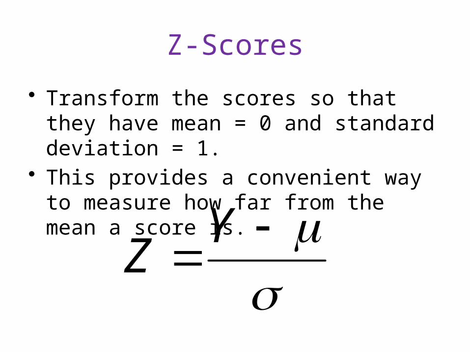
• Transform the scores so that they have mean = 0 and standard deviation = 1.
• This provides a convenient way to measure how far from the mean a score is.
Y
Z

Calculations on Y Scores
Y (Y - M) (Y - M)2 z*
5 +2 4 1.265
4 +1 1 0.633
3 0 0 0.000
2 -1 1 -0.633
1 -2 4 -1.265
Sum 15 0 10 0
Mean 3 0 2 = 2 0
*s = SQRT(10/4) = 1.581

Standard Scores
• Standard scores have a predetermined mean and standard deviation.
• Z scores are standard scores with mean 0 and standard deviation 1.
• IQ scores are standard scores with mean 100 and standard deviation 15.
• Each of the three sections of the SAT is standardized to mean 500 and standard deviation 100.

Convert from z to Other Standard Score
• Suzie Clueless has a raw score that is (z) two standard deviations below the mean. What is her IQ score?
• Standard Score = Standard Mean + (z score)(Standard Standard Deviation).
• IQ = 100 – 2(15) = 70. Suzie qualifies as a moron (IQ 51 to 70).

• Carlos Luis earned a intelligence test score 2.75 standard deviations above the mean. What is his IQ score?
• IQ = 100 + 2.75(15) = 141. Carlos qualifies as a genius.