dependence and order in families of archimedean copulas

File: 683J 164601 . By:CV . Date:06:01:97 . Time:13:47 LOP8M. V8.0. Page 01:01Codes: 4203 Signs: 2393 . Length: 50 pic 3 pts, 212 mm

Journal of Multivariate Analysis � MV1646

journal of multivariate analysis 60, 111�122 (1997)

Dependence and Order in Families ofArchimedean Copulas

Roger B. Nelsen*

Lewis 6 Clark College

The copula for a bivariate distribution function H(x, y) with marginal distribu-tion functions F (x) and G( y) is the function C defined by H(x, y)=C(F (x), G( y)).C is called Archimedean if C(u, v)=.&1(.(u)+.(v)), where . is a convex decreas-ing continuous function on (0, 1] with .(1)=0. A copula has lower tail dependenceif C(u, u)�u converges to a constant # in (0, 1] as u � 0+; and has upper taildependence if C� (u, u)�(1&u) converges to a constant $ in (0, 1] as u � 1& whereC� denotes the survival function corresponding to C. In this paper we developmethods for generating families of Archimedean copulas with arbitrary values of #and $, and present extensions to higher dimensions. We also investigate limitingcases and the concordance ordering of these families. In the process, we presentanswers to two open problems posed by Joe (1993, J. Multivariate Anal. 46262�282). � 1997 Academic Press

1. INTRODUCTION

The purpose of this paper is to present some methods for generatingparametric families of bivariate distribution functions which are ordered byconcordance and which possess a prescribed dependence structure knownas tail dependence. The concept of tail dependence for bivariate distribu-tion functions was introduced by Joe in [11], and is a property of thecopula of the distribution, i.e., the function C : [0, 1]2 � [0, 1]�d satisfyingH(x, y)=C(F(x), G( y)), where H is the bivariate distribution function oftwo random variables X and Y with marginal distribution functions F andG, respectively. A copula is itself a bivariate distribution function withmargins uniform on [0, 1]. For a general discussion of copulas and theirproperties, see [14, Chapter 6]. We will review the concepts of lower andupper tail dependence in copulas in Section 2.

article no. MV961646

1110047-259X�97 �25.00

Copyright � 1997 by Academic PressAll rights of reproduction in any form reserved.

Received March 2, 1995; revised August 14, 1996.

AMS 1991 subject classifications: primary 62E10; secondary 60E05, 62H05.Key words and phrases: Archimedean copula, bivariate distribution, multivariate distribu-

tion, concordance ordering, lower tail dependence, upper tail dependence.

* Fax: (503) 768-7668. E-mail: nelsen�lclark.edu.


In [11], Joe studied tail dependence and other properties of multivariatemixture families of distributions derived using Laplace transforms (also see[13]). Joe concluded his paper with the following statement:

In conclusion, some difficult open problems are:

1. Are there families of absolutely continuous multivariate copulas that have(i) simple forms, (ii) all bivariate margins in the same family, (iii) a wider rangeof dependence structures than those given [by multivariate mixtures], and(iv) bivariate tail dependence?

2. Is there a simple family of bivariate copulas with both upper and lower taildependence?

3. Are there general approaches other than the mixture or Laplace transformapproach? Note that for the Laplace transform approach, there does not seem tobe a way to tell from a family of [Laplace transforms] whether the resultingfamily of copulas will interpolate between independence and the Fre� chet upperbound.

A type of copula known as Archimedean can be used to address theseproblems, so we will begin the next section with a review of Archimedeancopulas and their properties. In Sections 3 and 4 we will illustrate methodsfor generating families of Archimedean copulas which do interpolatebetween independence and the Fre� chet upper bound (responding to Joe'sthird problem); and in Section 5 we will present methods for generatingfamilies of Archimedean copulas to answer positively the second question.In Section 6 we extend these methods to the multivariate case, and presentan example satifying three of the four conditions in Joe's first problem.

2. PRELIMINARIES

Let 8 denote the set of functions . : [0, 1] � [0, �] which are con-tinuous, strictly decreasing, convex, and for which .(0)=� and .(1)=0.Each . # 8 has an inverse .&1: [0, �] � [0, 1] which has the sameproperties, except .&1(0)=1 and .&1(�)=0. Each member of 8 generatesa copula C, that is, a bivariate distribution function with margins uniformon [0, 1] given by

C(u, v)=.&1(.(u)+.(v)), 0�u, v�1. (2.1)

These copulas are called Archimedean, and their properties are discussed in[6] and [7]. We call . a generator of C. The support of C is (0, 1]2, andC is absolutely continuous on (0, 1)2. An important subclass of 8 consistsof those elements . which have two continuous derivatives on (0, 1), with.$(t)<0 and ."(t)>0 for t # (0, 1). We shall denote this subclass as8 & C 2. Finally, if . is a generator of C, then so is c. for any positiveconstant c.

112 ROGER B. NELSEN


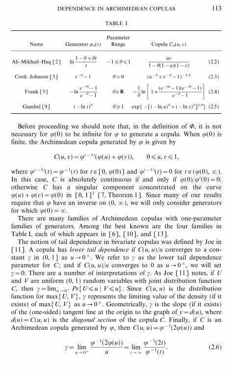
TABLE I

ParameterName Generator .%(t) Range Copula C%(u, v)

Ali�Mikhail�Haq [2] ln1&%+%t

t&1�%�1

uv1&%(1&u)(1&v)

(2.2)

Cook�Johnson [3] t&%&1 %>0 (u&%+v&%&1)&1�% (2.3)

Frank [5] &lne&%t&1e&%&1

% # R &1%

ln _1+(e&%u&1)(e&%v&1)

e&%&1 & (2.4)

Gumbel [9] (&ln t)% %�1 exp[&[(&ln u)%+(&ln v)%]1�%] (2.5)

Before proceeding we should note that, in the definition of 8, it is notnecessary for .(0) to be infinite for . to generate a copula. When .(0) isfinite, the Archimedean copula generated by . is given by

C(u, v)=.(&1)(.(u)+.(v)), 0�u, v�1,

where .(&1)(t)=.&1(t) for t # [0, .(0)] and .(&1)(t)=0 for t # (.(0), �).In this case, C is absolutely continuous if and only if .(0)�.$(0)=0;otherwise C has a singular component concentrated on the curve.(u)+.(v)=.(0) in [0, 1]2 [7, Theorem 1]. Since many of our resultsrequire that . have an inverse on (0, �), we will only consider generatorsfor which .(0)=�.

There are many families of Archimedean copulas with one-parameterfamilies of generators. Among the best known are the four families inTable I, each of which appears in [6], [10], and [13].

The notion of tail dependence in bivariate copulas was defined by Joe in[11]. A copula has lower tail dependence if C(u, u)�u converges to a con-stant # in (0, 1] as u � 0+. We refer to # as the lower tail dependenceparameter for C ; and if C(u, u)�u converges to 0 as u � 0+, we will set#=0. There are a number of interpretations of #. As Joe [11] notes, if Uand V are uniform (0, 1) random variables with joint distribution functionC, then #=limu � 0+ Pr[U�u | V�u]. Since C(u, u) is the distributionfunction for max[U, V ], # represents the limiting value of the density (if itexists) of max[U, V ] as u � 0+. Geometrically, # is the slope (if it exists)of the (one-sided) tangent line at the origin to the graph of y=d(u), whered(u)=C(u, u) is the diagonal section of the copula C. Finally, if C is anArchimedean copula generated by ., then C(u, u)=.&1(2.(u)) and

#= limu � 0+

.&1(2.(u))u

= limt � �

.&1(2t).&1(t)

. (2.6)

113DEPENDENCE IN ARCHIMEDEAN COPULAS


Similarly, a copula has upper tail dependence if C� (u, u)�(1&u) convergesto a constant $ in (0, 1] as u � 1&, where C� is the bivariate survival func-tion for C given by C� (u, v)=1&u&v+C(u, v). We will refer to $ as theupper tail dependence parameter for C, and if C� (u, u)�(1&u) converges to0 as u � 1&, we will set $=0. With U and V as in the preceding paragraph,$=limu � 1& Pr[U>u | V>u]. Since 1&C� (u, u) is the distribution func-tion for min[U, V ], $ represents the limiting value of the density (if itexists) of min[U, V ] as u � 1&. Geometrically, 2&$ is the slope (if itexists) of the (one-sided) tangent line to y=d(u) at (1, 1). If C is anArchimedean copula generated by ., then C� (u, u)=1&2+.&1(2.(u))and

$=2& limu � 1&

1&.&1(2.(u))1&u

=2& limt � 0+

1&.&1(2t)1&.&1(t)

. (2.7)

The notion of tail dependence is useful in the theory of extreme orderstatistics. As noted in [11], the condition $=0 is equivalent to the asymp-totic independence of Xmax and Ymax , where (Xi , Yi) is a sample from adistribution with copula C (when the marginal limiting extreme distribu-tions of Xmax and Ymax exist). Also note that upper tail dependence in thecopula is equivalent to lower tail dependence in the survival copula.

3. GENERATORS AND TAIL DEPENDENCE

In this section we study the relationship between the form of a generatorof an Archimedean copula and values of the tail dependence parameters #and $. However, we first present three properties of 8 which enable us toconstruct families of generators (and consequently families of Archimedeancopulas) from a single generator . in 8. Their proofs are trivial.

Property 1. Let . # 8, and let .;(t)=[.(t)] ;. Then .;(t) # 8 for all;�1.

Property 2. Let . # 8, and let .:(t)=.(t:). Then .:(t) # 8 for all: # (0, 1].

Property 3. Let . # 8 & C 2 such that t.$(t) is nondecreasing on (0, 1),and let .:(t)=.(t:). Then .:(t) # 8 & C 2 for all :>0.

In the sequel, for any . # 8, we will refer to a family of generators[.;(t) # 8 | .;(t)=[.(t)] ;] as a beta family associated with ., and a

114 ROGER B. NELSEN


family [.:(t) # 8 | .:(t)=.(t:)] as an alpha family associated with .. Forexample, the alpha family associated with .(t)=t&1&1 with :>0generates the Cook and Johnson family (2.3); and the beta familyassociated with .(t)=&ln t with ;�1 generates the Gumbel family (2.5).

If the copula C generated by . # 8 has lower tail dependence parameter# and upper tail dependence parameter $, then, as we shall see in the nexttwo theorems, it is easy to determine the tail dependence parameters for thecopulas generated by the alpha and beta families associated with .. But wemust first assume that # and $ exist for the copula C ; for it is easy to con-struct a . # 8 for which # (or $) does not exist. For example, let .&1 bethe piecewise linear function joining the points [(xn , yn) | n=0, 1, ...]where (x0 , y0)=(0, 1) and (xn , yn)=(2n&1, 2&w3n�2x) for n�1. Then .&1

is strictly decreasing and convex with .&1(0)=1 and .&1(�)=0, so that. # 8 and generates an Archimedean copula. However

.&1(22k).&1(22k&1)

=12

and.&1(22k+1)

.&1(22k)=

14

for k=1, 2, ...,

so that, using (2.6), #=limt � � .&1(2t)�.&1(t) does not exist. Indeed,using cubic splines, one can construct a C 2 function for .&1 with the sameproperties.

Theorem 1. Let . # 8 generate the copula C with lower tail dependenceparameter # # [0, 1] and upper tail dependence parameter $ # [0, 1]. Let.:(t)=.(t:), and further suppose that each .: generates a copula C: . ThenC: has lower and upper tail dependence parameters #: and $: , respectively,given by #:=#1�: and $:=$.

Proof. Since .&1: (t)=[.&1(t)]1�:, (2.6) yields

#:= limt � 0+

.&1: (2.:(t))

t= lim

t � 0+

[.&1(2.(t:))]1�:

[t:]1�: =#1�:.

Similarly, using (2.7), we have

2&$:= limt � 1&

1&.&1: (2.:(t))1&t

= limt � 1&

1&[.&1(2.(t:))]1�:

1&t

= limt � 1&

1&[.&1(2.(t))]1�:

1&t1�: .



Hence

2&$:

2&$= lim

t � 1&

1&[.&1(2.(t))]1�:

1&t1�: }1&t

1&[.&1(2.(t))]

= limu � 1&

1&u1�:

1&u} lim

t � 1&

1&t1&t1�:=1.

Thus $:=$ for :>0. K

Theorem 2. Let . # 8 generate the copula C with lower tail dependenceparameter # # [0, 1] and upper tail dependence parameter $ # [0, 1]. Let.;(t)=[.(t)] ;, ;�1. Then .;(t) generates a copula C; with lower taildependence parameter #;=#1�; and upper tail dependence parameter $;=2&(2&$)1�;.

Proof. Since .&1; (t)=.&1(t1�;), (2.6) yields

#;= limt � 0+

.&1; (2.;(t))

t= lim

t � 0+

.&1(21�;.(t))t

= limu � �

.&1(21�;u).&1(u)

.

Now let h(x)=limu � � .&1(2xu)�.&1(u) for x # [0, 1]. Then

h(x+y)= limu � �

.&1(2x+yu).&1(u)

= limu � �

.&1(2x2 yu).&1(2 yu)

}.&1(2 yu)

.&1(u)

= limv � �

.&1(2xv).&1(v)

} limu � �

.&1(2 yu).&1(u)

=h(x) h( y).

This is a variant of Cauchy's equation on the triangle 0�x�1, 0�y�1,0�x+y�1, the general solution of which is h(x)=ekx for some k [1].But #1�x=h(x) for x # (0, 1], hence #=#1=h(1)=ek so that h(x)=#x.Thus #;=h(1�;)=#1�;, as required.

Similarly, using (2.7), we have

2&$;= limt � 1&

1&.&1; (2.;(t))1&t

= limt � 1&

1&.&1(21�;.(t))1&t

= limu � 0+

1&.&1(21�;u)1&.&1(u)

.

Now let h(x)=limu � 0+ [1&.&1(2xu)]�[1&.&1(u)] for x # [0, 1] andrepeat the above argument to show that h(x)=(2&$)x. But 2&$1�x=h(x), so that 2&$;=h(1�;)=(2&$)1�;. K

116 ROGER B. NELSEN


4. LIMITING CASES AND ORDER

Let M, 6, and W denote the copulas of the Fre� chet upper bound, inde-pendence, and the Fre� chet lower bound, respectively; i.e., let M(u, v)=min[u, v], 6(u, v)=uv, and W(u, v)=max[u+v&1, 0]. In the nexttheorem, which follows directly from Propositions 4.2 and 4.3 in [6], wepresent sufficient conditions under which the family of copulas generatedby an alpha family of generators includes 6 as a limiting case; and suf-ficient conditions under which the family of copulas generated by a betafamily of generators includes M as a limiting case.

Theorem 3. (i) Let . # 8 & C 2 such that .$(1){0. Set .:(t)=.(t:)for : # (0, 1) and let C: denote the copula generated by .: . Thenlim: � 0+ C:(u, v)=6(u, v). (ii) Let . # 8 & C 2, set .;(t)=[.(t)]; for;�1, and let C; denote the copula generated by .; . Thenlim; � � C;(u, v)=M(u, v).

In passing we note that M, although a limiting case in a family ofArchimedean copulas, is not itself an Archimedean copula [7, 14].

Theorem 3 provides an answer to Joe's third open problem. Let. # 8 & C 2 and consider the two-parameter family of generators .:, ;(t)=.; b .:(t)=[.(t:)] ; for : # (0, 1) and ;�1. Then if C:, ; denotes thecopula generated by .:, ; , it follows that C0, 1=6 (where C0, ;(u, v)=lim: � 0+ C:, ;(u, v)) and C:, �=M. We present an explicit example in thenext section.

Note that since Theorem 3 only concerns bivariate copulas, it is in asense only a partial answer to Joe's third problem, and that one still doesnot know from the form of the generators of an arbitrary Archimedeanfamily whether M and 6 are limiting members of the family.

There does not seem to be a corresponding general result for W as amember or limiting case in families of copulas generated by either an alphaor beta family of generators.

A copula C2 is more concordant than (or more positively quadrantdependent than) C1 if C2(u, v)�C1(u, v) for all u, v # [0, 1], in which casewe write C2rC1 . The following two properties (which readily follow fromTheorem 3.1 in [6]) show that all beta families of generators, and manyalpha families, generate families of copulas which are ordered by concor-dance. In these cases, we have a natural interpretation of the parameter forthe family.

Property 4. Let . # 8, set .;(t)=[.(t)] ;, and let C; denote thecopula generated by .; for ;�1. Then ;2�;1 implies C;2

rC;1.



Property 5. Let . # 8, and let .:(t)=.(t:). Let A�(0, �) such thatif : # A then (i) .: # 8 and (ii) .([.&1(t)]%) is subadditive for all % # (0, 1).Then for :1 , :2 # A, :2�:1 implies C:2

rC:1.

An alternative form for condition (ii) in Property 5 above is: .$:�.: isnonincreasing in :.

However, not all alpha families of generators generate families of copulasordered by concordance. For example, if .(t)=ln((2�t)&1), then no twomembers of the family of copulas generated by .:(t)=ln((2�t:)&1) for: # (0, 1] are comparable; for it is easy to show that C:(u, v)�C:�2(u, v) ifand only if u:�2+v:�2�1.

5. AN EXAMPLE

As an application, consider the generator .(t)=t&1&1. This functiongenerates the copula C(u, v)=uv�(u+v&uv), which is a member of severalwell-known families of copulas, including those of Ali, Mikhail, and Haq(2.2) and Cook and Johnson (2.3). Using the properties and theorems inthe preceding sections, we can construct a two-parameter family of copulaswith generators given by .:, ;(t)=.; b .:(t)=(t&:&1) ;, :�0, ;�1.Explicitly, we have

C:, ;(u, v)=[[(u&:&1) ;+(v&:&1);]1�;+1]&1�:, u, v # [0, 1].

The tail dependence parameters for C(u, v)=uv�(u+v&uv) are #=1�2 and$=0; and so, by Theorems 1 and 2, the tail parameters for the copulasC:, ; generated by .:, ; are given by #:, ;=2&1�(:;) and $:, ;=2&21�;. Thispair of equations is invertible, thus to find a copula with a predeterminedlower tail dependence parameter # and upper tail dependence parameter $,set :=&ln(2&$)�ln # and ;=ln 2�ln(2&$). The one-parameter subfamilyC0, ; is the Gumbel family (2.5), while the one-parameter subfamily C:, 1 isthe Cook and Johnson family (2.3). This family also appears in [12] as thefamily of survival copulas for a ``random hazards'' bivariate Weibull model.

As noted earlier, this family of copulas interpolates between 6 and M,since C0, 1=6 and C:, �=M. From Properties 4 and 5 in the precedingsection, it is easy to show that this family of copulas is concordanceordered by both : and ; ; i.e., if :2�:1 and ;2�;1 ; then C:2 , ;2

rC:1 , ;1.

Hence every member of this family is positively quadrant dependent, sinceC0, 1=6. Furthermore, the family is also concordance ordered by the tailparameters # and $, since :2�:1 and ;2�;1 imply that the correspondingvalues of # and $ satisfy #2�#1 and $2�$1 , and conversely.

Thus this family provides a positive answer to the second of Joe's openproblems [11] from Section 1: Is there a simple family of bivariate copulas

118 ROGER B. NELSEN


with both upper and lower tail dependence? Indeed, there are one-parameter subfamilies which accomplish the same end��simply set;=:+1, : # [0, �); or ;=1�(1&:), : # [0, 1), for example.

Of course, other families can be readily constructed using other gener-ators in 8. Examples include .(t)=ln(1&ln t), .(t)=1�t&t, .(t)=exp[(1�t)&1]&1, and so on. Many such generators generate copulas forwhich both # and $ are zero; but note that even in this event, Theorem 2quarantees that members of the family of copulas generated by a betafamily of generators will have positive upper tail dependence.

6. MULTIVARIATE EXTENSIONS

The natural extension of (2.1) to n dimensions is

Cn(u1 , u2 , ..., un)=.&1(.(u1)+.(u2)+ } } } +.(un)),

0�u1 , u2 , ..., un�1. (6.1)

[In this section, an integer superscript such as n on C, #, or $ will denotedimension rather than exponentiation.] Of course, Cn may not be ann-dimensional copula (briefly, n-copula), i.e., an n-dimensional distributionfunction whose univariate margins are uniform on (0, 1). What propertiesof . (or .&1) will insure that Cn given by (6.1) is an n-copula? The answeris given in the following theorem.

Theorem 4 [14, Theorem 6.3.6]. Let . # 8. Then Cn given by (6.1) isan n-copula for all n�2 if and only if .&1 is completely monotonic in(0, �), i.e., .&1 is real-analytic and satisfies

(&1)k d k

dtk .&1(t)�0

for all t # (0, �) and k=0, 1, 2, ... .

This theorem can be easily extended to cover the cases in which .&1 ism-monotonic in (0, �), i.e., the cases in which only the first m derivativesof .&1 alternate in sign. In such cases, Cn given by (6.1) is an n-copula for2�n�m.

Note that the functions Cn in (6.1) are the serial iterates [14] of C ; that is,if we set C 2(u1 , u2)=C(u1 , u2)=.&1(.(u1)+.(u2)), then Cn(u1 , u2 , ..., un)=C(Cn&1(u1 , u2 , ..., un&1), un) for n�3. However, we must mention that thistechnique for creating multivariate distribution functions��endowing abivariate copula with multidimensional margins��generally fails [8]. For



example, W(W(u1 , u2), u3)=max[u1+u2+u3&2, 0] is not a distributionfunction.

We are now in a position to demonstrate that the 2-copulas generated bybeta families of generators in Section 3 extend, via (6.1), to n dimensions.The following theorem, which is an immediate consequence of Criterion 2in [4, Section XIII.4], accomplishes this.

Theorem 5. Let . # 8 such that .&1 is completely monotonic in (0, �).Let .;(t)=[.(t)]; for ;�1. Then .&1

; is completely monotonic in (0, �).

Again consider the two-parameter family of generators .:, ;(t)=.; b .:(t)=[.(t:)] ; for :>0 and ;�1. If .&1

: is completely monotonic in(0, �), then Theorem 5 guarantees that .&1

:, ; is completely monotonic in(0, �), and hence, by Theorem 4, .:, ; generates an n-copula of theform given by (6.1). For example, if we again set .(t)=t&1&1, it is easyto show that for :>0, .&1

: (t)=(1+t)&1�: is completely monotonic in(0, �), and thus .:, ;(t)=(t&:&1) ; generates a two-parameter family ofn-copulas

Cn:, ;(u1 , u2 , ..., un)={_ :

n

i=1

(u&:i &1) ;&

1�;

+1=&1�:

,

0�u1 , u2 , ..., un�1, (6.2)

for :>0, ;�1, and for each n�2.The definitions of upper and lower tail dependence extend to n dimen-

sions. Paralleling the definitions in Section 2, we will say that an n-copulaCn has lower tail dependence parameter #n if Cn(u, u, ..., u)�u converges toa constant #n in [0, 1] as u � 0+; and has upper tail dependence parameter$n if C� n(u, u, ..., u)�(1&u) converges to a constant $n in [0, 1] as u � 1&.Now let . # 8 such that .&1 is completely monotonic in (0, �), and con-sider the n-copulas Cn

; generated by .;(t)=[.(t)] ; for ;�1, and then-copulas Cn

: generated by .:(t)=.(t:) for :>0 (here we must assumethat .&1

: is completely monotonic in (0, �) for :>0). Let #n: and #n

; denotethe lower tail dependence parameters and let $n

: and $n; denote the upper

tail dependence parameters for Cn: and Cn

; , respectively. Let #n and $n nowdenote the lower and upper tail dependence parameters, respectively, forthe n-copula Cn generated by . ; i.e., the n-copula given by (6.1). Usingmethods similar to those in the proofs of Theorems 1 and 2, it is easy toshow that #n

:=(#n)1�:, $n:=$n, #n

;=(#n)1�;, and

$n;= :

n

k=1

(&1)k+1 \nk+ _ :

k

j=1

(&1) j+1 \ kj + $ j&

1�;

(6.3)

(where we take $1#1).

120 ROGER B. NELSEN


As a final example, let #n:, ; and $n

:, ; denote the lower and upper taildependence parameters, respectively, for the two parameter family ofn-copulas given by (6.2). Then #n

:, ;=(#n)1�(:;) and $n:, ;=$n

; given by (6.3).When .(t)=t&1&1, the k-copulas (for k=2, 3, ..., n) generated by . havelower tail dependence parameters #k=1�k for k=2, 3, ...,n ; and upper taildependence parameters $k=0 for k=2, 3, ..., n. Hence the two-parameterfamily of n-copulas in (6.2), which have generators .:, ;(t)=(t&:&1) ;,have lower tail dependence parameters #n

:, ;=n&1�(:;) and upper taildependence parameters $n

:, ;=�nk=1 (&1)k+1 ( n

k) k1�; (using the notationof finite differences, this last result can be expressed more concisely as$n

:, ;=(&1)n+1 2n01�;). Although this family does not provide a positiveanswer to the first open problem in [11] (since its dependence structure islimited by the fact that it is a family with exchangeable or symmetricdependence), it is a family of absolutely continuous multivariate copulaswith a simple form, all bivariate margins in the same family (indeed, hereall k-variate margins are in the same family, k=2, 3, ..., n&1), andbivariate tail dependence (these in fact have k-variate lower and upper taildependence).

ACKNOWLEDGMENTS

The author thanks J. Chen, M. J. Frank, and G. A. Fredricks for their valuable assistancewith several sections in this paper and to an editor and two referees for their insightful com-ments and suggestions.

REFERENCES

[1] Acze� l, J. (1966). Lectures on Functional Equations and Their Applications. AcademicPress, New York.

[2] Alli, M. M., Mikhail, N. N., and Haq, M. S. (1978). A class of bivariate distributionsincluding the bivariate logistic. J. Multivariate Anal. 8 405�412.

[3] Cook, R. D., and Johnson, M. E. (1981). A family of distributions for modeling non-elliptically symmetric multivariate data. J. Roy. Statist. Soc. B. 53 377�392.

[4] Feller, W. (1971). An Introduction to Probability Theory and Its Applications, Vol. II,2nd ed. Wiley, New York.

[5] Frank, M. J. (1979). On the simultaneous associativity of F(x, y) and x+y&F(x, y).Aequationes Math. 19 194�226.

[6] Genest, C., and MacKay, R. J. (1986). Copules archime� diennes et familles de loisbidimensionelles dont les marges sont donne� es. Canad. J. Statist. 14 145�159.

[7] Genest, C., and MacKay, R. J. (1986). The joy of copulas: Bivariate distributions withuniform marginals. Amer. Statist. 40 280�285.

[8] Genest, C., Quesada Molina, J. J., and Rodr@� guez Lallena, J. A. (1995). De l'im-possibilite� de construire des lois a� marges multidimensionnelles donne� es a� partir decopules. C. R. Acad. Sci. Paris Se� r. I Math. 320 723�726.



[9] Gumbel, E. J. (1960). Distributions des valeurs extremes en plusieurs dimensions. Publ.Inst. Statist. Univ. Paris 9 171�173.

[10] Hutchinson, T. P., and Lai, C. D. (1990). Continuous Bivariate Distributions, Emphasis-ing Applications. Rumsby, Adelaide.

[11] Joe, H. (1993). Parametric families of multivariate distributions with given margins.J. Multivariate Anal. 46 262�282.

[12] Lu, J.-C., and Bhattacharyya, G. K. (1990). Some new constructions of bivariateWeibull models. Ann. Inst. Statist. Math. 42 543�559.

[13] Marshall, A. W., and Olkin, I. (1988). Families of multivariate distributions. J. Amer.Statist. Assoc. 83 834�841.

[14] Schweizer, B., and Sklar, A. (1983). Probabilistic Metric Spaces. Elsevier, New York.

122 ROGER B. NELSEN

dependence and order in families of archimedean copulas

Documents