Sampling Archimedean copulas

Marius Hofert

Preprint Series: 2007-10

Fakultat fur Mathematik und Wirtschaftswissenschaften

UNIVERSITAT ULM

Sampling Archimedean copulas

Marius Hofert1

Version of 2008-02-28

Abstract

This paper addresses the problem of efficiently sampling exchangeable and nested

Archimedean copulas, with specific focus on large dimensions, where methods in-

volving generator derivatives, such as the conditional distribution method, are not

applicable. Additionally, new conditions under which Archimedean copulas can be

mixed to construct nested Archimedean copulas are presented. Moreover, for some

Archimedean families, direct sampling algorithms are given. For other families, sam-

pling algorithms based on numerical inversion of Laplace transforms are suggested.

For this purpose, the Fixed Talbot, Gaver Stehfest, Gaver Wynn rho, and Laguerre

series algorithm are compared in terms of precision and runtime. Examples are

given, including both exchangeable and nested Archimedean copulas.

1 Introduction

A distinct property of Archimedean copulas is that they are fully specified by somegenerator function. Important for various modeling purposes is that Archimedean cop-ulas are flexible to capture various dependence structures, e.g. concordance and taildependence, which makes them suitable for modeling extreme events. Recently, nestedArchimedean copulas gained interest as they extend exchangeable Archimedean copu-las to allow for asymmetries, an important property for several financial applications.Sampling such copulas is required in practical applications but also interesting from atheoretical perspective.

Different methodologies for sampling bivariate Archimedean copulas are known, e.g. theconditional distribution method or an approach based on the probability integral trans-formation, see Embrechts, Lindskog, McNeil (2001). The former generalizes to mul-tivariate exchangeable Archimedean copulas, see Embrechts, Lindskog, McNeil (2001),and requires the knowledge of the first d derivatives of the generator of the d-dimensionalArchimedean copula under consideration. Wu, Valdez, Sherris (2006) generalize the lat-ter for sampling multivariate exchangeable Archimedean copulas and the correspondingalgorithm involves the first d − 1 derivatives of the Archimedean generator. A similarapproach is taken in Whelan (2004). Recently, McNeil, Nešlehová (2007) have presented

1 Universität Ulm, Institut für Angewandte Analysis, Helmholtzstraße 18, 89069 Ulm, marius.

hofert@uni-ulm.de

This paper is part of the author’s dissertation, which is carried out under the supervision of Prof.

Dr. Ulrich Stadtmüller.

1

1 Introduction

a sampling algorithm for multivariate exchangeable Archimedean copulas which only in-volves the first d− 2 derivatives of the generator. A common drawback of all these sam-pling algorithms is that one has to know the involved generator derivatives. This prob-lem becomes especially critical when nested Archimedean copulas are considered. Theconditional distribution method is computationally impractical due to complex mixedderivatives, which is already a challenge for small dimensions, see Savu, Trede (2006)for this approach. Whelan (2004) tackles the problem of sampling nested Archimedeancopulas by taking a similar direction as for sampling exchangeable Archimedean copulas.This approach also requires high order derivatives, however, with respect to much lessvariables than the conditional distribution approach. Applicability of all these algorithmsis strongly limited by the number of dimensions.

Considering the subclass of completely monotone Archimedean generators slightly simpli-fies the theory, in that we have the well-known relation of generators to Laplace-Stieltjestransforms of distribution functions on the positive real line. Knowing the distributioncorresponding to such a generator, Marshall, Olkin (1988) presented a sampling algo-rithm for exchangeable Archimedean copulas which does not require the knowledge ofthe copula density and is therefore applicable to large dimensions. Algorithms for thefew multivariate exchangeable Archimedean copulas that are straightforward to samplein large dimensions exploit the knowledge of the inverse Laplace-Stieltjes transform, seeJoe (1997), page 375, for four Archimedean families. A generalization of the idea ofMarshall, Olkin (1988) to nested Archimedean copulas, and an elegant sampling algo-rithm was provided by McNeil (2007). However, for sampling in large dimensions, onlyone family is feasible, namely the Gumbel family. The reason for this is the lack ofknowledge of the inverse Laplace-Stieltjes transforms of the generators that are requiredfor this algorithm. Further, no certain class of generators is known which can be nestedsuch that sampling for its members is directly possible. Moreover, no example of gener-ators belonging to different Archimedean families that can be mixed to build a nestedArchimedean copula is known, which is interesting for practical applications, e.g. toallow for different kinds of tail dependence. The goal of this paper is to overcome someof these difficulties.

This paper is organized as follows. In Section 2 we present and discuss algorithmsbased on the inverse Laplace-Stieltjes transform for sampling exchangeable and nestedArchimedean copulas. We also present techniques for a verification of the sufficient condi-tion developed by McNeil (2007) for nested Archimedean structures to be proper copulas.We further obtain several conditions which guarantee multivariate nested Archimedeancopulas. For some families we obtain efficient sampling algorithms, including the cases ofnested Ali-Mikhail-Haq, nested Frank, and nested Joe copulas. The section closes withseveral examples of generators belonging to different Archimedean families that can bemixed to construct nested Archimedean copulas. In Section 3 we briefly introduce nu-merical inversion methods of Laplace transforms and present the Fixed Talbot, GaverStehfest, Gaver Wynn rho, and Laguerre series algorithm. Section 4 investigates andcompares these algorithms in terms of precision and runtime using the Clayton family

2

2 Sampling exchangeable and nested Archimedean copulas

as reference. In Section 5 we present several examples that tackle unsolved problems.Finally, Section 6 concludes.

2 Sampling exchangeable and nested Archimedean copulas

2.1 Exchangeable Archimedean copulas

An Archimedean generator is a nonincreasing, continuous function ψ0 : [0,∞] → [0, 1]which satisfies ψ0(0) = 1, ψ0(∞) = 0 and is strictly decreasing on [0, inf{t : ψ0(t) = 0}].As McNeil, Nešlehová (2007) show, an Archimedean generator defines an exchangeable

Archimedean copula, given by

C(u) = C(u1, . . . , ud;ψ0) = ψ0(ψ−10 (u1) + · · ·+ ψ−1

0 (ud)), u ∈ [0, 1]d, (1)

if and only if ψ0 is d-monotone, i.e. ψ0 is continuous on [0,∞], has derivatives up tothe order d − 2 satisfying (−1)k dk

dtkψ0(t) ≥ 0 for any k ∈ {0, . . . , d− 2}, t ∈ (0,∞), and

(−1)d−2 dd−2

dtd−2ψ0(t) being nonincreasing and convex on (0,∞). Unless stated otherwisewe concentrate on the case where ψ0 is completely monotone, i.e. (−1)k dk

dtkψ0(t) ≥ 0 for

any k ∈ N0, t ∈ (0,∞). The advantage of this condition is that we can exploit therelation of ψ0 to Laplace-Stieltjes transforms, see Kimberling’s Theorem below. Someproperties of completely monotone functions are summarized in the following lemma.

Lemma 2.1(1) Completely monotone functions are closed under multiplications and linear combi-

nations with positive coefficients, i.e. if f and g are completely monotone, so are fgand λf + µg for any λ, µ ≥ 0.

(2) If f is completely monotone, g nonnegative, and g′ completely monotone, then f ◦ gis completely monotone.

(3) Let f be nonnegative, such that f ′ is completely monotone, then 1/f is completelymonotone.

(4) If f is absolutely monotone, i.e. f is continuous on [0,∞] and satisfies dk

dtkf(t) ≥ 0

for any k ∈ N0, t ∈ (0,∞), and g completely monotone, then f ◦ g is completelymonotone.

(5) Let f be a Laplace-Stieltjes transform. Then fα is completely monotone for anyα ∈ (0,∞) if and only if (− log f)′ is completely monotone.

ProofFor Parts (1) and (4) of Lemma 2.1, see Widder (1946), page 145. Part (2) may be foundin Feller (1971), page 441. Part (3) is a straightforward application of Part (2). Part (5)is proven in Joe (1997), page 374. �

Kimberling (1974) gave the following necessary and sufficient condition for an Archime-dean generator to define a proper exchangeable Archimedean copula for any dimensionlarger than or equal to two.

3

2.1 Exchangeable Archimedean copulas

Theorem 2.2 (Kimberling)Let ψ0 : [0,∞] → [0, 1] be continuous and strictly decreasing with ψ0(0) = 1 andψ0(∞) = 0. Then (1) is a copula for any d ≥ 2 if and only if ψ0 is completely monotone.

According to the if part of Kimberling’s Theorem, we may find generators ψ0 for ex-changeable Archimedean copulas by using continuous functions ψ0 : [0,∞] → [0, 1],satisfying ψ0(0) = 1, ψ0(∞) = 0 and being completely monotone. In the sequel, theclass of all such functions ψ0 will be referred to as Ψ∞. Bernstein’s Theorem, seeFeller (1971), page 439, establishes the link between completely monotone functions andLaplace-Stieltjes transforms. It is the building block for efficient sampling algorithms forexchangeable and nested Archimedean copulas, especially in large dimensions.

Theorem 2.3 (Bernstein)A function ψ0 on [0,∞] is the Laplace-Stieltjes transform of a distribution function ifand only if ψ0 is completely monotone and ψ0(0) = 1.

The following algorithm for sampling a d-dimensional exchangeable Archimedean copulawith generator ψ0 is due to Marshall, Olkin (1988), where LS−1(ψ0) denotes the inverseLaplace-Stieltjes transform of ψ0.

Algorithm 1 (Marshall, Olkin)(1) Sample V0 ∼ F0 = LS−1(ψ0).

(2) Sample i.i.d. Xi ∼ U [0, 1], i ∈ {1, . . . , d}.

(3) Return (U1, . . . , Ud), where Ui = ψ0(− log(Xi)/V0), i ∈ {1, . . . , d}.

If we know how to sample F0, Algorithm 1 provides a powerful tool for sampling ex-changeable Archimedean copulas. This algorithm is especially efficient in large dimen-sions, as only d + 1 random numbers are required for generating a d-dimensional ob-servation. More precisely, only one sample V0 ∼ F0 is required, independent of thedimension.

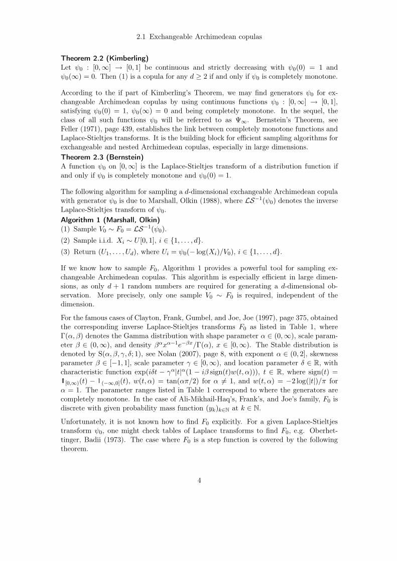
For the famous cases of Clayton, Frank, Gumbel, and Joe, Joe (1997), page 375, obtainedthe corresponding inverse Laplace-Stieltjes transforms F0 as listed in Table 1, whereΓ(α, β) denotes the Gamma distribution with shape parameter α ∈ (0,∞), scale param-eter β ∈ (0,∞), and density βαxα−1e−βx/Γ(α), x ∈ [0,∞). The Stable distribution isdenoted by S(α, β, γ, δ; 1), see Nolan (2007), page 8, with exponent α ∈ (0, 2], skewnessparameter β ∈ [−1, 1], scale parameter γ ∈ [0,∞), and location parameter δ ∈ R, withcharacteristic function exp(iδt − γα|t|α(1 − iβ sign(t)w(t, α))), t ∈ R, where sign(t) =1[0,∞)(t) − 1(−∞,0](t), w(t, α) = tan(απ/2) for α 6= 1, and w(t, α) = −2 log(|t|)/π forα = 1. The parameter ranges listed in Table 1 correspond to where the generators arecompletely monotone. In the case of Ali-Mikhail-Haq’s, Frank’s, and Joe’s family, F0 isdiscrete with given probability mass function (yk)k∈N at k ∈ N.

Unfortunately, it is not known how to find F0 explicitly. For a given Laplace-Stieltjestransform ψ0, one might check tables of Laplace transforms to find F0, e.g. Oberhet-tinger, Badii (1973). The case where F0 is a step function is covered by the followingtheorem.

4

2.1 Exchangeable Archimedean copulas

Family ϑ0 ψ0(t) F0

Ali-Mikhail-Haq [0, 1) 1−ϑ0

et−ϑ0yk = (1− ϑ0)ϑ0

k−1, k ∈ N

Clayton (0,∞) (1 + t)−1/ϑ0 Γ(1/ϑ0, 1)

Frank (0,∞) −(log(e−t(e−ϑ0 − 1) + 1))/ϑ0 yk = (1−e−ϑ0 )k

kϑ0, k ∈ N

Gumbel [1,∞) exp(−t1/ϑ0) S(1/ϑ0, 1, (cos(π

2ϑ0))ϑ0 , 0; 1)

Joe [1,∞) 1− (1− e−t)1/ϑ0 yk = (−1)k+1(1/ϑ0

k

)

, k ∈ N

Table 1 Archimedean families with corresponding parameter ranges, generators, andinverse Laplace-Stieltjes transforms.

Theorem 2.4Let ψ0 be the Laplace-Stieltjes transform of the distribution function F0 and let F (x) =∑

∞

k=0 yk1[xk,∞)(x), with 0 < x0 < x1 < . . . and yk > 0, k ∈ N0, with∑

∞

k=0 yk = 1.Then

F0 ≡ F ⇔ ψ0(t) =

∞∑

k=0

yke−xkt, t ∈ [0,∞].

ProofThe only if part of the claim follows from the definition of Laplace-Stieltjes transforms.For the if part of the statement we note that the Laplace-Stieltjes transform of F att ∈ [0,∞] equals

∑

∞

k=0 yke−xkt, which in turn equals ψ0, the Laplace-Stieltjes transform

of F0. The uniqueness theorem of inverse Laplace-Stieltjes transforms, see Doetsch(1970), page 32, implies that F0 ≡ F up to a set of Lebesgue measure zero, whichimplies F0 ≡ F . �

An application of Theorem 2.4 leads to the probability mass functions of F0 for the fam-ilies of Ali-Mikhail-Haq, Frank, and Joe as listed in Table 1. The computation involvesa geometric series expansion for Ali-Mikhail-Haq’s, a logarithmic series expansion forFrank’s, and a binomial series expansion for Joe’s generator.

Now assume as given an Archimedean generator ψ ∈ Ψ∞, for which we know F =LS−1(ψ) explicitly. An interesting question is, if we can transform ψ to a generatorψ0 in such a way that we still know F0 = LS−1(ψ0) in terms of F . The followingtheorem concerns such a result, where we note that the involved generator ψ0 is simplya shifted and appropriately scaled ψ. In the sequel, we therefore refer to the resultingArchimedean copulas simply as shifted Archimedean copulas.

Theorem 2.5Let ψ ∈ Ψ∞ with F = LS−1(ψ). For a given h ∈ [0,∞), let ψ0(t) = ψ(t + h)/ψ(h) forany t ∈ [0,∞]. Then

(a) ψ0(t), t ∈ [0,∞], is completely monotone and ψ0(0) = 1.

(b) F0 = LS−1(ψ0) is given by F0(x) = (F (0) +∫ x0 e

−hu dF (u))/ψ(h), x ∈ [0,∞).

5

2.2 Nested Archimedean copulas

(c) If F admits a density f , then F0 admits the exponentially tilted density f0(x) =e−hxf(x)/ψ(h), x ∈ [0,∞).

ProofAs ψ ∈ Ψ∞, Part (a) directly follows. For Part (b), let g1(x) = e−hxF (x), x ∈ [0,∞).From (6) at the beginning of Section 3, we know that

(L(F0))(t) =ψ0(t)

t=ψ(t+ h)

t+ h

t+ h

tψ(h)= (L(F ))(t+ h) (L(g2))(t)

= (L(g1))(t) (L(g2))(t), t ∈ [0,∞],

with g2(x) = (δ(x) + h)/ψ(h), x ∈ [0,∞), where δ denotes the Dirac delta function.Hence, L(F0) = L(g1 ∗ g2), which implies F0 = (g1 ∗ g2). Solving this convolution usingpartial integration for Riemann-Stieltjes integrals leads to the desired result. Part (c)follows from (b). �

The following rejection algorithm, see Devroye (1986), page 42, can be applied to samplethe exponentially tilted density given in Part (c) of Theorem 2.5. However, we notethat this approach can be slow, as the expected number of iterations in the algorithm is1/ψ(h).

Algorithm 2Repeatedly sample V ∼ f and U ∼ U [0, 1], until U ≤ e−hV , then return V .

2.2 Nested Archimedean copulas

The symmetry inherent in exchangeable Archimedean copulas is a strong restriction,especially for large dimensions, as the dependence among all components is identical;in other words, all common marginal distribution functions of the same dimension areequal. One way to extend exchangeable Archimedean copulas to allow for asymmetry isto use an important property of Archimedean copulas, namely associativity.

Extending the notation introduced in (1), we write

C(u1, . . . , ud;ψ0, . . . , ψd−2) = ψ0(ψ−10 (u1) + ψ−1

0 (C(u2, . . . , ud;ψ1, . . . , ψd−2))) (2)

for any d ≥ 3, ui ∈ [0, 1], i ∈ {1, . . . , d}. The structure recursively defined via (2) iscalled fully nested Archimedean copula. For d = 3, this corresponds to

C(u) = C(u1, C(u2, u3;ψ1);ψ0) = ψ0(ψ−10 (u1) + ψ−1

0 (ψ1(ψ−11 (u2) + ψ−1

1 (u3)))). (3)

Note that a d-dimensional fully nested Archimedean copula is able to capture d − 1different pairwise dependencies, i.e. it possesses d − 1 different bivariate margins. Inreal-world applications, it is often sufficient and convenient to combine the structures (1)

6

2.2 Nested Archimedean copulas

and (2). The resulting copulas are called partially nested Archimedean copulas. Althoughnesting is possible at any level, for notational convenience, we only consider the case

C(u) = C(C(u11, . . . , u1d1;ψ1), . . . , C(us1, . . . , usds

;ψs);ψ0)

= ψ0(ψ−10 (ψ1(ψ

−11 (u11) + · · ·+ ψ−1

1 (u1d1))) + . . .

+ ψ−10 (ψs(ψ

−1s (us1) + · · ·+ ψ−1

s (usds))))

= ψ0

( s∑

i=1

ψ−10

(

ψi

( di∑

j=1

ψ−1i (uij)

)))

, (4)

uij ∈ I, i ∈ {1, . . . , s}, j ∈ {1, . . . , di}, where s is the number of sectors and d =∑s

i=1 di

is the dimension. This copula allows for modeling s+ 1 different pairwise dependencies.The four-dimensional example with two sectors is given by

C(u) = C(C(u11, u12;ψ1), C(u21, u22;ψ2);ψ0)

= ψ0(ψ−10 (ψ1(ψ

−11 (u11) + ψ−1

1 (u12))) + ψ−10 (ψ2(ψ

−12 (u21) + ψ−1

2 (u22)))).

According to their structures, fully and partially nested Archimedean copulas are simplyreferred to as nested (or hierarchical) Archimedean copulas. The following theorem, seeMcNeil (2007), gives a sufficient condition for (2) being a proper copula. Similarly, for(4) being a proper copula, a sufficient condition is that nodes of the form ψ−1

0 ◦ ψi forany i ∈ {1, . . . , s} have completely monotone derivatives.

Theorem 2.6 (McNeil)Let ψi ∈ Ψ∞ for i ∈ {0, . . . , d − 2} such that ψ−1

k ◦ ψk+1 have completely monotonederivatives for any k ∈ {0, . . . , d− 3}, then C(u1, . . . , ud;ψ0, . . . , ψd−2) is a copula.

Based on the idea of Algorithm 1, McNeil (2007) proposed a sampling strategy fornested Archimedean copulas. The principal idea of this algorithm is to apply Algorithm1 iteratively. In each step, one samples the distribution functions associated with theLaplace-Stieltjes transforms of certain generators. These generators are, due to thenodes, of the form ψi,j(t;V0) = exp(−V0ψ

−1i ◦ ψj(t)), where V0 is a given sample of the

distribution function F0 from an earlier step, or outer structure, and i and j refer to thenode under consideration. For (2), a recursive algorithm is given as follows.

Algorithm 3 (McNeil)(1) Sample V0 ∼ F0 = LS−1(ψ0).

(2) Sample (X2, . . . ,Xd) ∼ C(u2, . . . , ud;ψ0,1(·;V0), . . . , ψ0,d−2(·;V0)).

(3) Sample X1 ∼ U [0, 1].

(4) Return (U1, . . . , Ud), where Ui = ψ0(− log(Xi)/V0), i ∈ {1, . . . , d}.

The following algorithm of McNeil (2007) is for sampling the partially nested Archime-dean copula (4).

7

2.2 Nested Archimedean copulas

Algorithm 4 (McNeil)(1) Sample V0 ∼ F0 = LS−1(ψ0).

(2) For i ∈ {1, . . . , s}, sample (Xi1, . . . ,Xidi) ∼ C(ui1, . . . , uidi

;ψ0,i(·;V0)) using Algo-rithm 1.

(3) Return (U11, . . . , Usds), where Uij = ψ0(− log(Xij)/V0), i ∈ {1, . . . , s}, j ∈ {1, . . . ,

di}.

Assume as given Archimedean generators ψi belonging to the Gumbel family with pa-rameters ϑi, i ∈ {0, . . . , d− 2}, satisfying 1 ≤ ϑ0 ≤ · · · ≤ ϑd−2. By Joe (1997), page 375,it follows that (2) and (4) are proper copulas. It is readily verified that the generatorsψ0,j(t;V0), j ∈ {1, . . . , d − 2}, are given by ψ0,j(t;V0) = exp(−V0t

α), α = ϑ0/ϑj, whichcorresponds to a S(α, 1, (cos(π

2α)V0)1/α, 0; 1) distribution. For Step (2) of Algorithm 3

or 4, one may alternatively sample the copula generated by exp(−tα), corresponding toa S(α, 1, (cos(π

2α))1/α, 0; 1) distribution, since for an Archimedean generator ψ(t), ψ(ct)generates the same copula. Hence for Gumbel’s family, the algorithm works efficiently.Unfortunately, this is the only known case where sampling a nested Archimedean copulaof large dimension is feasible.

Verifying the condition of Theorem 2.6 for a nested Archimedean copula with generatorsbelonging to the same family is often unproblematic. Joe (1997), page 375, alreadygave sufficient conditions for the families of Clayton, Frank, Gumbel, and Joe. Foreither of these, if ψ0 and ψ1 are generators for two members of the involved family withparameters ϑ0 and ϑ1, respectively, then (ψ−1

0 ◦ψ1)′ is completely monotone if ϑ0 ≤ ϑ1.

Table 2 lists the Archimedean generators whose inverses are completely monotone onthe given parameter ranges that may be found in Nelsen (1998), pages 94-97, withcorresponding numbering. For Clayton’s family, we use a different generator. Further,this table contains conditions on the parameters ϑ0 and ϑ1 under which (ψ−1

0 ◦ ψ1)′ is

completely monotone, where ϑi denotes the parameter of ψi as before. All conditionsmay be obtained by applying Lemma 2.1 and checking no. 14 additionally involves thebinomial theorem.

For the families of Ali-Mikhail-Haq, Frank, and Joe, F0 = LS−1(ψ0) is discrete. In thefollowing theorem, we show that for these Archimedean families, F0,1 = LS−1(ψ0,1) isalso discrete with given distribution function.

Theorem 2.7(a) If ψi(t) = (1 − ϑi)/(e

t − ϑi), t ∈ [0,∞], with ϑi ∈ [0, 1) for i ∈ {0, 1} such thatϑ0 ≤ ϑ1, then ψ0,1(t;V0), with V0 ∈ N, has inverse Laplace-Stieltjes transformF0,1(x) =

∑

∞

k=V0yk1[xk,∞)(x) with

xk = k, yk =ck−V0

2

ck1

(

k − 1

k − V0

)

, k ∈ N\{1, . . . , V0 − 1},

where c1 = (1 − ϑ0)/(1 − ϑ1) and c2 = (ϑ1 − ϑ0)/(1 − ϑ1). Hence, for the nestedArchimedean family of Ali-Mikhail-Haq, F0,1 is discrete with probability densityfunction yk at k ∈ N\{1, . . . , V0 − 1}.

8

2.2 Nested Archimedean copulas

Family ϑi ψi(t) (ψ−10 ◦ ψ1)

′ c.m.

1 (0,∞) (1 + t)−1/ϑi ϑ0, ϑ1 ∈ (0,∞) : ϑ0 ≤ ϑ1

3 [0, 1) (1− ϑi)/(et − ϑi) ϑ0, ϑ1 ∈ [0, 1) : ϑ0 ≤ ϑ1

4 [1,∞) exp(−t1/ϑi) ϑ0, ϑ1 ∈ (0,∞) : ϑ0 ≤ ϑ1

5 (0,∞) −(log(e−t(e−ϑi − 1) + 1))/ϑi ϑ0, ϑ1 ∈ [1,∞) : ϑ0 ≤ ϑ1

6 [1,∞) 1− (1− e−t)1/ϑi ϑ0, ϑ1 ∈ [1,∞) : ϑ0 ≤ ϑ1

12 [1,∞) (1 + t1/ϑi)−1 ϑ0, ϑ1 ∈ [1,∞) : ϑ0 ≤ ϑ1

13 [1,∞) exp(1− (1 + t)1/ϑi) ϑ0, ϑ1 ∈ [1,∞) : ϑ0 ≤ ϑ1

14 [1,∞) (1 + t1/ϑi)−ϑi ϑ0, ϑ1 ∈ [1,∞) : ϑ0 ∈ N, ϑ1/ϑ0 ∈ N

19 (0,∞) ϑi/ log(t+ eϑi ) ϑ0, ϑ1 ∈ (0,∞) : ϑ0 ≤ ϑ1

20 (0,∞) (log(t+ e))−1/ϑi ϑ0, ϑ1 ∈ (0,∞) : ϑ0 ≤ ϑ1

Table 2 Completely monotone Archimedean generators of Nelsen (1998), pages 94-97,with parameter ranges such that the condition of Theorem 2.6 holds.

(b) If ψi(t) = −(log(e−t(e−ϑi − 1) + 1))/ϑi, t ∈ [0,∞], with ϑi ∈ (0,∞) for i ∈ {0, 1}such that ϑ0 ≤ ϑ1, then ψ0,1(t;V0), with V0 ∈ N, has inverse Laplace-Stieltjestransform F0,1(x) =

∑

∞

k=V0yk1[xk,∞)(x) with

xk = k, yk =ck2

cV0

1

V0∑

j=0

(

V0

j

)(

jϑ0/ϑ1

k

)

(−1)j+k, k ∈ N\{1, . . . , V0 − 1},

where ci = 1 − e−ϑi for i ∈ {1, 2}. Hence, for the nested Archimedean family ofFrank, F0,1 is discrete with probability density function yk at k ∈ N\{1, . . . , V0−1}.

(c) If ψi(t) = 1 − (1 − e−t)1/ϑi , t ∈ [0,∞], with ϑi ∈ [1,∞) for i ∈ {0, 1} such thatϑ0 ≤ ϑ1, then ψ0,1(t;V0), with V0 ∈ N, has inverse Laplace-Stieltjes transformF0,1(x) =

∑

∞

k=V0yk1[xk,∞)(x) with

xk = k, yk =

V0∑

j=0

(

V0

j

)(

jϑ0/ϑ1

k

)

(−1)j+k, k ∈ N\{1, . . . , V0 − 1}.

Hence, for the nested Archimedean family of Joe, F0,1 is discrete with probabilitydensity function yk at k ∈ N\{1, . . . , V0 − 1}.

ProofFor Part (a), an application of the binomial series theorem leads to

ψ0,1(t;V0) =

∞∑

k=V0

ck−V0

2

ck1

(

k − 1

k − V0

)

e−kt.

The conditions of Theorem 2.4 are easily verified. For Part (b), apply the binomialtheorem and the binomial series theorem to observe that

ψ0,1(t;V0) =

∞∑

k=0

(

ck2cV0

1

V0∑

j=0

(

V0

j

)(

jϑ0/ϑ1

k

)

(−1)j+k

)

e−kt,

9

2.2 Nested Archimedean copulas

which we interpret as∑

∞

k=0 yke−kt. Checking yk ≥ 0 for k ∈ N0 is done by computing

the corresponding generating function and by showing that it is absolutely monotone.Showing yk = 0 for k ∈ {0, . . . , V0−1} is done by an inductive argument. Part (c) workssimilarly to Part (b). �

Instead of considering each generator individually, the following general result is shownunder which we can construct a parametric family that can be nested, starting from anygiven completely monotone Archimedean generator.

Theorem 2.8Let ψ ∈ Ψ∞. If ψi(t) = ψ((cϑi + t)1/ϑi − c), t ∈ [0,∞], with ϑi ∈ [1,∞) for i ∈ {0, 1}and c ∈ [0,∞), then

(a) ψi is completely monotone and ψi(0) = 1 for i ∈ {0, 1}.

(b) (ψ−10 ◦ψ1)(t) = (cϑ1 +t)ϑ0/ϑ1−cϑ0 , t ∈ [0,∞], so (ψ−1

0 ◦ψ1)′ is completely monotone

if ϑ0 ≤ ϑ1.

ProofBoth statements are applications of Lemma 2.1. �

Remark 2.9Based on the generator ψ(t) = 1/(1+t) we obtain families no. 1, for c = 1, i.e. Clayton’sfamily, and no. 12, for c = 0, from Theorem 2.8. Further, with ψ(t) = 1/(1 + log(1 + t))we obtain an equivalent generator for family no. 19, for c = 1. We notice the frequentappearance of the generator ψ(t) = 1/(1 + t), a fact which might explain Nelsen’s openquestion no. 5. in Nelsen (2005). Based on the generator of the independent copula,ψ(t) = e−t, we obtain families no. 4, for c = 0, i.e. Gumbel’s family, and no. 13, forc = 1. Also note that all generators of the form ψi(t) = ψ( 1

ϑilog(1 + t)) for a ψ ∈ Ψ∞

and ϑi ∈ (0,∞) are special cases of Theorem 2.8.

Sampling in the framework of Theorem 2.8 involves the inner distribution function F0,1 =LS−1(ψ0,1), where ψ0,1(t;V0) = exp(−V0((h+ t)α− hα)), α = ϑ0/ϑ1, and h = cϑ1 . Notethat this is a shifted Archimedean generator, so we may apply Theorem 2.5, wherethe involved density f is the density of a S(α, 1, (cos(π

2α)V0)1/α, 0; 1) distribution as for

Gumbel’s family. Again, instead of sampling the copula generated by ψ0,1, we may aswell sample the copula generated by exp(−((h + t)α − hα)), where h = V0

1/αh. In thiscase, the involved density f is the density of a S(α, 1, (cos(π

2α))1/α, 0; 1) distributionand sampling the exponentially tilted Stable density f0,1 corresponding to F0,1 withAlgorithm 2 requires exp(V0c

ϑ0) iterations on average.

For a generator ψ of a two-dimensional Archimedean copula, it is known that ψ0(t) =(ψ(t))1/α for any α ∈ (0, 1] as well as ψ1(t) = ψ(t1/β) for any β ∈ [1,∞) generatetwo-dimensional Archimedean copulas again. Families generated by ψ0 are referred toas inner power families, the ones generated by ψ1 are called outer power families. Aninteresting question is, if and how these concepts generalize to our multivariate setting.

10

2.2 Nested Archimedean copulas

For outer power families, Theorem 2.8 affirms both questions, choose c = 0. Further,the simulation of nested Archimedean copulas based on an outer power family of a givengenerator ψ involves generators of the form ψ0,1(t;V0) = exp(−V0t

α), α = ϑ0/ϑ1. Hence,one can sample a Stable distribution as for Gumbel’s family. As an example, considergenerator no. 12, which is an outer power family based on the Clayton generator no.1 with parameter equal to one. For inner power families, note that all generators ofTable 2 fulfill that ψ0(t) = (ψ(t))1/α is completely monotone for any α ∈ (0,∞). If oursole knowledge is that ψ is completely monotone, we still have that ψ0 is completelymonotone if 1/α ∈ N, by Lemma 2.1 (4). Unfortunately, no general result on when wecan construct nested Archimedean copulas based on inner power families is known. Notethat the sufficient condition of Theorem 2.6 is usually not fulfilled, e.g. consider thegenerator ψ(t) = (2et − 1)−1 of Ali-Mikhail-Haq’s copula with parameter equal to onehalf and let ψi(t) = (ψ(t))1/ϑi with ϑi ∈ (0, 1] for i ∈ {0, 1} such that ϑ0/ϑ1 = 1/2. Thisimplies (ψ−1

0 ◦ ψ1)′′(log 5) > 0, so (ψ−1

0 ◦ ψ1)′ is not completely monotone.

Generators ψ0 which are zero at some finite point can also be brought into play, as thefollowing result shows, where ψ−1

0 (0) is defined as inf{t : ψ0(t) = 0}.

Theorem 2.10For i ∈ {0, 1}, let ψi : [0,∞] → [0, 1] with ψi(0) = 1 and ψ−1

i (0) < ∞ be completely

monotone on [0, ψ−1i (0)]. If ψi(t) = ψi(ψ

−1i (0)(1 − e−t)), t ∈ [0,∞], for i ∈ {0, 1}, then

(a) ψi is completely monotone and ψi(0) = 1 for i ∈ {0, 1}.

(b) (ψ−10 ◦ψ1)(t) = − log(1−ψ−1

0 (ψ1((1−e−t)ψ−1

1 (0)))/ψ−10 (0)), t ∈ [0,∞], so (ψ−1

0 ◦ψ1)′

is completely monotone if (1 − ψ−10 (ψ1((1 − e−t)ψ−1

1 (0)))/ψ−10 (0))α is completely

monotone for any α ∈ (0,∞).

ProofBoth parts are applications of Lemma 2.1. �

Remark 2.11The families of Frank, no. 5, and Joe, no. 6, fit in the framework of Theorem 2.10,

as we can see by choosing ψi(t) = (− log(e−ϑi + t))/ϑi with ϑi ∈ (0,∞) for i ∈ {0, 1},and ψi(t) = 1 − t1/ϑi with ϑi ∈ [1,∞) for i ∈ {0, 1}, respectively, where each generatoris defined to be zero outside the unit interval. For these families, Part (b) of Theorem2.10 is verified in Joe (1997), page 375. Another application of Theorem 2.10 is givenby family no. 3, i.e. Ali-Mikhail-Haq’s family. In this case, we use ψi(t) = (1 − t)(1 −ϑi)/(1−ϑi(1− t)) for t ∈ [0, 1] and zero else, with ϑi ∈ [0, 1) for i ∈ {0, 1}. Further notethat Part (b) of Theorem 2.10 is fulfilled by Lemma 2.1 Parts (1) and (3).

If generators of different Archimedean families are mixed, the sufficient condition ofTheorem 2.6 does not always hold. For example, if ψ0 and ψ1 are generators for Clayton’sand Gumbel’s copula, respectively, a simple calculation shows that the condition (ψ−1

0 ◦ψ1)

′ being completely monotone is not fulfilled for any parameter choice. Further, (ψ−11 ◦

ψ0)′ being completely monotone only holds if the parameter of Gumbel’s copula equals

11

3 Numerical inversion of Laplace transforms

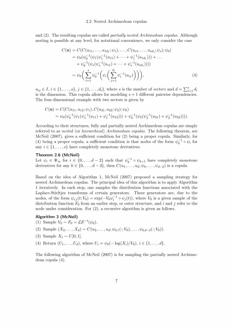
one, i.e. if ψ1 generates the independent copula. Table 3 lists all combinations of thecompletely monotone generators of Nelsen (1998), pages 94-97, which result in propernested Archimedean copulas according to the sufficient condition of Theorem 2.6.

Family combination ϑ0 ϑ1 (ψ−10 ◦ ψ1)

′(t) c.m.

(1,12) (0,∞) [1,∞) ϑ0 ∈ (0, 1](1,14) (0,∞) [1,∞) ϑ0ϑ1 ∈ (0, 1](1,19) (0,∞) (0,∞) ϑ0 ∈ (0, 1](1,20) (0,∞) (0,∞) ϑ0 ≤ ϑ1

(3,1) [0, 1) (0,∞) ϑ1 ∈ [1,∞)(3,19) [0, 1) (0,∞) any ϑ0, ϑ1

(3,20) [0, 1) (0,∞) any ϑ0, ϑ1

Table 3 Proper family combinations and corresponding param-eter ranges for the Archimedean families of Nelsen(1998), pages 94-97.

3 Numerical inversion of Laplace transforms

In this section, we present numerical algorithms for inverting Laplace transforms tosample exchangeable and nested Archimedean copulas. This is especially encouragedby the fact that runtime for sampling Archimedean copulas primarily depends on thenumber of sectors and hardly on the dimension of the copula, since uniform randomnumbers are easily generated. Assume as given an Archimedean generator ψ ∈ Ψ∞

with

ψ(t) =

∫

∞

0e−tx dF (x), t ∈ [0,∞), (5)

and let the distribution corresponding to F be denoted by P. For (L(F ))(t), i.e. theLaplace transform of F at t, an application of Tonelli’s Theorem leads to

t(L(F ))(t) = t

∫

∞

0e−txF (x) dx = t

∫

∞

0e−tx

∫ x

0dP(u) dx

=

∫

∞

0

∫

∞

ute−tx dx dP(u) =

∫

∞

0e−tu dP(u) =

∫

∞

0e−tu dF (u)

= ψ(t), t ∈ [0,∞).

Hence, in terms of Laplace transforms, F can be written as

F (x) = (L−1(ψ(t)/t))(x), x ∈ [0,∞). (6)

Our suggestion in the following section is to compute (6) numerically. For the requiredinversion of Laplace transforms, many algorithms are known, see Valkó, Vojta (2001). We

12

3.1 Fixed Talbot, Gaver Stehfest, Gaver Wynn rho, and Laguerre series algorithm

shortly review the Fixed Talbot, Gaver Stehfest, Gaver Wynn rho, and Laguerre seriesalgorithm, however, we note that these algorithms should rather serve as examples, asnumerical inversion of Laplace transforms is an ill-posed problem, meaning that there isno uniformly best algorithm for all Laplace transforms.

3.1 Fixed Talbot, Gaver Stehfest, Gaver Wynn rho, and Laguerre seriesalgorithm

The Fixed Talbot algorithm is an improved version of the original algorithm of Talbot(1979). The principal idea of this algorithm is to numerically evaluate the Bromwichinversion integral for Laplace transforms and to overcome some technical difficulties byusing a certain choice for the contour; an excellent reference is Abate, Valkó (2004).In terms of our problem (6), the Fixed Talbot algorithm is efficiently implemented asfollows, where we compute as much as possible only once, and as little as required forevery value x where we would like to evaluate F . The approximation of F is denoted byF and still depends on the choice of the parameter M of this algorithm, where Abate,Valkó (2004) suggest an implementation in which the number of decimal digits that canbe represented in the mantissa should be at least M in order to prevent round-off errors.

Algorithm 5 (Fixed Talbot)(1) Choose M ∈ N.

(2) Compute c = e0.4M

2M .

(3) For k ∈ {1, . . . ,M − 1}, compute ϑk = kπM , sk = 0.4Mϑk(cot(ϑk) + i), σk = 1 +

i(ϑk + (ϑk cot(ϑk)− 1) cot(ϑk)) and finally wk = esk σk

sk.

(4) For any x, return F (x) = cψ(0.4M/x) + 0.4x

M−1∑

k=1

Re(wkxψ(sk/x)).

Note that the Fixed Talbot algorithm requires ψ at complex arguments. The extensionof ψ to the complex plane is usually quite simple, as the Laplace-Stieltjes transformof F is a holomorphic function on the right half-plane U defined by the abscissa ofconvergence. It coincides with ψ(s) (ψ considered as a function with domain C) on thenonnegative real line intersected with U . Therefore, it suffices to find c ∈ R such thatψ(s) is holomorphic for any s ∈ C with Re(s) > c, as ψ(s) is then the unique extensionof ψ(t) to C by the identity theorem for holomorphic functions.

Another theoretical inversion formula for Laplace transforms is the Post-Widder formula,see Widder (1946), page 277, which uses derivatives of the given Laplace transform.Gaver (1966) obtained a similar formula, where derivatives are replaced by finite differ-ences. For approximating the inverse Laplace transform F , he started with the deltaconvergent sequence

δn(x, t) =(2n)!

n!(n− 1)!

log 2

x2−n t

x (1− 2−tx )n

13

3.1 Fixed Talbot, Gaver Stehfest, Gaver Wynn rho, and Laguerre series algorithm

and computed the so-called Gaver functionals

F (x) =

∫

∞

0δn(x, t)F (t) dt =

(2n)!

n!(n− 1)!

log 2

x

n∑

k=0

(

n

k

)

(−1)k(L(F ))

(

(n+ k)log 2

x

)

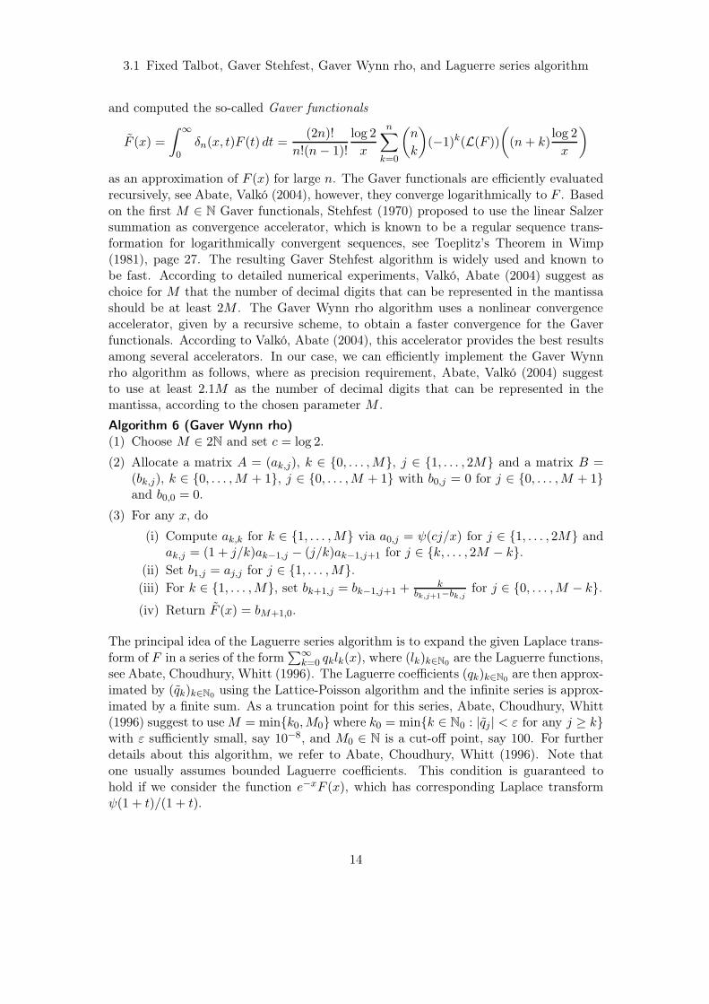
as an approximation of F (x) for large n. The Gaver functionals are efficiently evaluatedrecursively, see Abate, Valkó (2004), however, they converge logarithmically to F . Basedon the first M ∈ N Gaver functionals, Stehfest (1970) proposed to use the linear Salzersummation as convergence accelerator, which is known to be a regular sequence trans-formation for logarithmically convergent sequences, see Toeplitz’s Theorem in Wimp(1981), page 27. The resulting Gaver Stehfest algorithm is widely used and known tobe fast. According to detailed numerical experiments, Valkó, Abate (2004) suggest aschoice for M that the number of decimal digits that can be represented in the mantissashould be at least 2M . The Gaver Wynn rho algorithm uses a nonlinear convergenceaccelerator, given by a recursive scheme, to obtain a faster convergence for the Gaverfunctionals. According to Valkó, Abate (2004), this accelerator provides the best resultsamong several accelerators. In our case, we can efficiently implement the Gaver Wynnrho algorithm as follows, where as precision requirement, Abate, Valkó (2004) suggestto use at least 2.1M as the number of decimal digits that can be represented in themantissa, according to the chosen parameter M .

Algorithm 6 (Gaver Wynn rho)(1) Choose M ∈ 2N and set c = log 2.

(2) Allocate a matrix A = (ak,j), k ∈ {0, . . . ,M}, j ∈ {1, . . . , 2M} and a matrix B =(bk,j), k ∈ {0, . . . ,M + 1}, j ∈ {0, . . . ,M + 1} with b0,j = 0 for j ∈ {0, . . . ,M + 1}and b0,0 = 0.

(3) For any x, do

(i) Compute ak,k for k ∈ {1, . . . ,M} via a0,j = ψ(cj/x) for j ∈ {1, . . . , 2M} andak,j = (1 + j/k)ak−1,j − (j/k)ak−1,j+1 for j ∈ {k, . . . , 2M − k}.

(ii) Set b1,j = aj,j for j ∈ {1, . . . ,M}.

(iii) For k ∈ {1, . . . ,M}, set bk+1,j = bk−1,j+1 + kbk,j+1−bk,j

for j ∈ {0, . . . ,M − k}.

(iv) Return F (x) = bM+1,0.

The principal idea of the Laguerre series algorithm is to expand the given Laplace trans-form of F in a series of the form

∑

∞

k=0 qklk(x), where (lk)k∈N0are the Laguerre functions,

see Abate, Choudhury, Whitt (1996). The Laguerre coefficients (qk)k∈N0are then approx-

imated by (qk)k∈N0using the Lattice-Poisson algorithm and the infinite series is approx-

imated by a finite sum. As a truncation point for this series, Abate, Choudhury, Whitt(1996) suggest to useM = min{k0,M0} where k0 = min{k ∈ N0 : |qj | < ε for any j ≥ k}with ε sufficiently small, say 10−8, and M0 ∈ N is a cut-off point, say 100. For furtherdetails about this algorithm, we refer to Abate, Choudhury, Whitt (1996). Note thatone usually assumes bounded Laguerre coefficients. This condition is guaranteed tohold if we consider the function e−xF (x), which has corresponding Laplace transformψ(1 + t)/(1 + t).

14

4 Comparison of the algorithms

4 Comparison of the algorithms

In this section, we apply the Fixed Talbot, Gaver Stehfest, Gaver Wynn rho, and La-guerre series algorithm to evaluate F0 for Clayton’s family with parameter ϑ0 = 0.8,where we have a closed-form solution as reference. This corresponds to a Kendall’stau of 0.2857, which seems realistic for many applications. We compare the algorithmsaccording to precision and runtime.

4.1 Precision and runtime

In order to compare the precision of the different algorithms, we evaluated the involvedGamma distribution function F0 at 10, 000 equally spaced points, ranging from 0.001 to10, the set of these points is denoted by P . As F0(0.001) is close to zero and F0(10) isclose to one, these values represent the overall approximation of F0 very well. Precisionis measured using the maximal relative error MXRE. We consider a numerical procedurefor inverting Laplace transforms to be accurate enough for our sampling problem (6) ifMXRE satisfies

MXRE(x) = maxx∈P

∣

∣

∣

∣

F0(x)− F0(x)

F0(x)

∣

∣

∣

∣

< 0.0001. (7)

We further report the mean relative error MRE, defined as

MRE =1

|P |

∑

x∈P

∣

∣

∣

∣

F0(x)− F0(x)

F0(x)

∣

∣

∣

∣

.

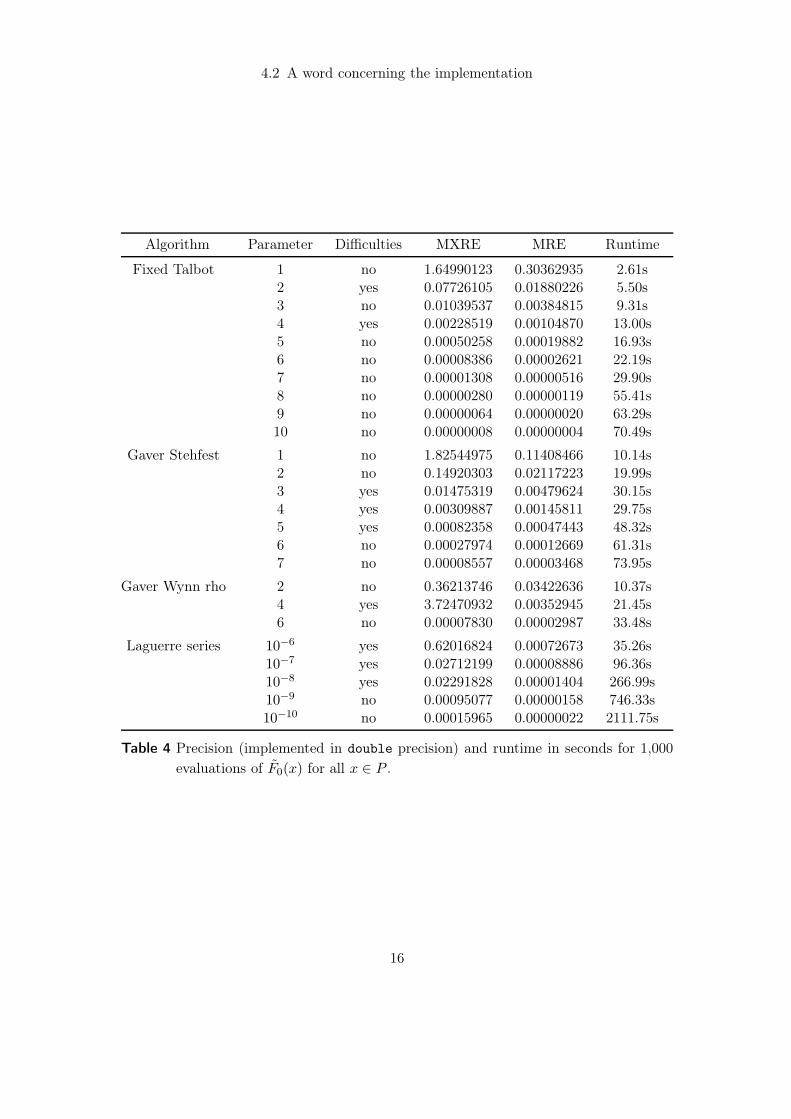
Table 4 presents the results of our investigation for all four algorithms. The parameterchoices for the algorithms are reported, which is M for the Fixed Talbot, Gaver Stehfest,and Gaver Wynn rho algorithm (chosen such that the precision requirements of Abate,Valkó (2004) hold) and ε for the Laguerre series algorithm. For the latter we do notuse the bound M0 in order to obtain a better insight in the precision of this algorithm.We further report eventual numerical difficulties if observed, i.e. values F0(x) whichare not in the unit interval for at least one x ∈ P . Finally, MXRE and MRE, aswell as runtimes for 1,000 evaluations of F0(x) for all points x ∈ P , are reported. Inour study, the Fixed Talbot and Gaver Wynn rho algorithms perform best. For bothalgorithms, the smallest M that meets criterion (7) is M = 6 and the correspondingruntimes for 10,000,000 function evaluations are comparably small. Especially the FixedTalbot algorithm achieves excellent precision in small runtime.

4.2 A word concerning the implementation

All numerical experiments are run on a node containing two AMD Opteron 252 processors(2.6 GHz) with 8 GB RAM as part of a Linux cluster. The algorithms are implemented

15

4.2 A word concerning the implementation

Algorithm Parameter Difficulties MXRE MRE Runtime

Fixed Talbot 1 no 1.64990123 0.30362935 2.61s2 yes 0.07726105 0.01880226 5.50s3 no 0.01039537 0.00384815 9.31s4 yes 0.00228519 0.00104870 13.00s5 no 0.00050258 0.00019882 16.93s6 no 0.00008386 0.00002621 22.19s7 no 0.00001308 0.00000516 29.90s8 no 0.00000280 0.00000119 55.41s9 no 0.00000064 0.00000020 63.29s10 no 0.00000008 0.00000004 70.49s

Gaver Stehfest 1 no 1.82544975 0.11408466 10.14s2 no 0.14920303 0.02117223 19.99s3 yes 0.01475319 0.00479624 30.15s4 yes 0.00309887 0.00145811 29.75s5 yes 0.00082358 0.00047443 48.32s6 no 0.00027974 0.00012669 61.31s7 no 0.00008557 0.00003468 73.95s

Gaver Wynn rho 2 no 0.36213746 0.03422636 10.37s4 yes 3.72470932 0.00352945 21.45s6 no 0.00007830 0.00002987 33.48s

Laguerre series 10−6 yes 0.62016824 0.00072673 35.26s10−7 yes 0.02712199 0.00008886 96.36s10−8 yes 0.02291828 0.00001404 266.99s10−9 no 0.00095077 0.00000158 746.33s10−10 no 0.00015965 0.00000022 2111.75s

Table 4 Precision (implemented in double precision) and runtime in seconds for 1,000

evaluations of F0(x) for all x ∈ P .

16

5 Examples

in C/C++ and compiled using GCC 3.3.3 (SuSE Linux) with option -O2 for code opti-mization. Under double precision, the number of base-10 digits that can be representedin the mantissa is 15, reported by the function digits10 of the C/C++ library limits.The command gettimeofday is used to measure runtime as wall-clock time. For gener-ating uniform random numbers we use an implementation of the Mersenne Twister byWagner (2003).

In order to find the quantile of a realization U ∼ U [0, 1] close to one, we proceed asfollows: If a numerical algorithm is not able to find the corresponding quantile, asthe computed values F (x) for reasonable large x do not reach U , we use truncation.For this, we specify a maximal value xmax, where F is evaluated. F (xmax) is thenused as truncation point. If U ∈ [0, F (xmax)], a root finding procedure is used to findthe U -quantile, otherwise F (xmax) is returned. For numerical root finding, we use thefunction nag_zero_cont_func_bd_1 of the Numerical Algorithms Group (NAG) andfor each numerical experiment, we give our choices of the corresponding parametersxtol and ftol. Beside truncation, more sophisticated methods, e.g. transformations orasymptotics in the tail, may be applied.

5 Examples

In this section, we present several examples of how exchangeable and nested Archimedeancopulas can be sampled based on the studied techniques. For all examples, we usethree, ten, and one hundred dimensions, involving only one level of nesting, however, wenote that all algorithms are applicable to sample more complex hierarchies, due to therecursive character of Algorithm 3. We further remark that for small dimensions, theconditional distribution method or other sampling algorithms may be faster; the reasonwhy we investigate the three-dimensional case is to give justification for correctness of thegenerated random numbers. For this task, each dimension is subdivided into five equally-spaced bins. The corresponding grid partitions the three-dimensional unit cube into 125cubes. For every three-dimensional example, 1,000 sets of samples, each of size 100,000,are taken and the p-value of the Kolmogorov-Smirnov test based on the 1,000 χ2 teststatistics is reported. For each example, all bins have expected number of observationsgreater than or equal to ten, being a rule of thumb for the χ2 test. Note that plots of theapproximations F0 and F0,1 may also serve as quality checks for detecting major flawsof numerical inversion algorithms. Whenever we sample an outer distribution functionF0, we plot F0(x) for all x ∈ P , and for an inner distribution function F0,1, we checkplots of F0,1 for reasonable realizations V0 from the outer distribution function F0. Theplots are presented for the nested (Ali-Mikhail-Haq,Clayton) copula. We further reportruntimes based on samples of size 100,000.

17

5.1 An exchangeable power Clayton copula

5.1 An exchangeable power Clayton copula

Consider the generator ψ0(t) = (ψ(t1/β))1/α, where ψ(t) = 1/(1+ t), i.e. ψ generates theClayton copula with parameter equal to one. In this case, ψ0(t) is completely monotonefor any α ∈ (0, 1] and β ∈ [1,∞). For our example, we choose α = 0.5 and β = 1.5. Foraccessing F0, we use the Fixed Talbot algorithm with M = 6, xtol = 10−8, and ftol =10−8. As truncation point, we choose xmax = 1016, resulting in F0(xmax) = 0.999996. Weobtain 0.51 as p-value of the Kolmogorov-Smirnov test and the pairwise sample versionsof Kendall’s tau are given by τ1,2 = 0.4667, τ1,3 = 0.4650, and τ2,3 = 0.4685, whichare close to the theoretical value 0.4666. Runtimes for generating 100,000 observationsof these three-, ten-, and one hundred-dimensional exchangeable power Clayton copulasare given by 16.16s, 16.76s, and 21.54s, respectively. We note that runtime is mainlydetermined by the evaluation of F0.

5.2 A nested outer power Clayton copula

Again, we consider ψ from Clayton’s family with parameter equal to one. We thenconstruct an outer power family based on this generator, i.e. we use the generatorsψi(t) = ψ(t1/ϑi), i ∈ {0, 1}, with ϑ0 = 1.1, ϑ1 = 1.5, and construct nested Archimedeancopulas with dimensions (1,2), (5,5), and (50,50), where the notation (1,2) correspondsto the three-dimensional structure as given in (3), and the cases (5,5) and (50,50) areconstructed accordingly, involving only larger dimensions for the nonsectorial and thesector part. For this nested outer power copula, we apply the Fixed Talbot algorithmwith M = 6, xmax = 108 (resulting in F0(xmax) = 0.999996), xtol = 10−8, and ftol = 0for sampling F0. As the inner distribution function F0,1 corresponds to a known Stabledistribution, we do not need to apply a numerical inversion algorithm for sampling F0,1.As p-value of the Kolmogorov-Smirnov test we obtain 0.81 and the sample versionsof Kendall’s tau are given by τ1,2 = 0.3945, τ1,3 = 0.3924, and τ2,3 = 0.5561. Thecorresponding theoretical values are τ1,2 = τ1,3 = 0.3939 and τ2,3 = 0.5556, where theformer reflect the concordance of pairs of random variables with bivariate Archimedeancopula generated by ψ0 with parameter ϑ0 and the latter reflects the concordance ofa pair of random variables with bivariate Archimedean copula generated by ψ1 withparameter ϑ1. Runtimes for generating 100,000 observations of these three-, ten-, andone hundred-dimensional nested outer power Clayton copulas are given by 10.89s, 11.39s,and 17.57s, respectively.

5.3 A nested Ali-Mikhail-Haq copula

We now examine nested Archimedean copulas of the types (1,2), (5,5), and (50,50), asbefore, constructed using generators of the Archimedean family of Ali-Mikhail-Haq withparameters ϑ0 = 0.5 and ϑ1 = 0.9, where F0 is a geometric distribution. For samplingF0,1, we precompute its values until F0,1(x) ≥ 1 − ε, where ε is chosen as 10−8. The

18

5.4 A nested (Ali-Mikhail-Haq,Clayton) copula

p-value of the Kolmogorov-Smirnov test for the three-dimensional copula is reportedas 0.76 and the sample versions of Kendall’s tau are given by τ1,2 = 0.1264, τ1,3 =0.1292, and τ2,3 = 0.2792, corresponding to the theoretical values τ1,2 = τ1,3 = 0.1288and τ2,3 = 0.2782. As runtimes for these three-, ten-, and one hundred-dimensionalnested Ali-Mikhail-Haq copulas, we obtain 0.17s, 0.32s, and 2.40s, even outperformingthe runtimes for nested Gumbel copulas of the same types (0.51s, 0.85s, and 5.46s), forwhich one only has to sample Stable distributions.

5.4 A nested (Ali-Mikhail-Haq,Clayton) copula

As before, consider nested Archimedean copulas of the form (1,2), (5,5), and (50,50),where ψ0 is now a generator of Ali-Mikhail-Haq’s copula with parameter ϑ0 = 0.8 andψ1 is a generator of Clayton’s copula with parameter ϑ1 = 2. For the resulting nestedmixed Archimedean copulas, we sample the known distribution function F0 for Step(1) of Algorithm 3, and use the Fixed Talbot algorithm with M = 6, xmax = 104,F0,1(xmax) = 0.999996, xtol = 10−8, and ftol = 0 for sampling F0,1. The p-valueof the Kolmogorov-Smirnov test is reported as 0.53 and sample versions of Kendall’stau are given by τ1,2 = 0.2349, τ1,3 = 0.2358, and τ2,3 = 0.5029, corresponding to thetheoretical values τ1,2 = τ1,3 = 0.2337 and τ2,3 = 0.5. Runtimes for generating 100,000observations of these three-, ten-, and one hundred-dimensional nested (Ali-Mikhail-Haq,Clayton) copulas are given by 7.54s, 7.78s, and 11.58s, respectively. Figure 1 showsplots of F0,1(x) for the samples V0 ∈ {1, 2, 5, 10} of F0 and a scatter plot matrix for thethree-dimensional nested (Ali-Mikhail-Haq,Clayton) copula based on 1,000 observations.We especially emphasize the different tail behavior of the generated data.

0.0

0.2

0.4

0.6

0.8

1.0

0.0 0.5 1.0 1.5 2.0

(1)

(2)

(3)

(4)

x

F0,1(x

)

(1) V0 = 1(2) V0 = 2(3) V0 = 5(4) V0 = 10 Component 1

Component 2

Component 3

Figure 1 F0,1(x) with V0 ∈ {1, 2, 5, 10} (left) and a scatter plot matrix (right) for thenested (Ali-Mikhail-Haq,Clayton) copula.

19

6 Conclusion

We close this section by advising the reader to carefully use numerical inversion algo-rithms for Laplace transforms. Usually, these algorithms involve assumptions on theunderlying functions, which are not easily checked or which can not be checked at all,as these functions are not directly given. Further, there is no guarantee that algorithmswhich worked well in the presented examples, are applicable to others. Checking thequality of an approximation F0 to an outer distribution function F0 is comparably easy,however, sampling an inner distribution function F0,1 using a numerical inversion pro-cedure for Laplace transforms requires the algorithm to work accurately for all samplesV0 from F0.

6 Conclusion

In this paper, we gave sufficient conditions for the parameters of the completely monotonegenerators listed in Nelsen (1998), pages 94-97, such that nested Archimedean copulascan be constructed. Many of these generators fall into two categories, for which Theo-rems 2.8 and 2.10 addressed conditions for nesting. We could generally relate the innerdistribution function F0,1 involved in Theorem 2.8 to an exponentially tilted Stable dis-tribution by introducing shifted Archimedean generators. As a special case, we furtherobtained that outer power families extend to multivariate Archimedean copulas and thatthe inner distribution function F0,1 corresponds to a Stable distribution, independent ofthe family under consideration. We also obtained probability mass functions for the innerdistribution functions F0,1 for the families of Ali-Mikhail-Haq, Frank, and Joe. Theseresults allow to directly sample the corresponding nested Archimedean copulas. For sam-pling exchangeable and nested Archimedean copulas where F0 or F0,1 can not be directlysampled, we suggested an approach based on numerical inversion of Laplace transforms.Using such algorithms for sampling exchangeable and nested Archimedean copulas inlarge dimensions is motivated by the fact that we only need a comparably small amountof random variates from F0 and F0,1. We investigated the Fixed Talbot, Gaver Stehfest,Gaver Wynn rho, and Laguerre series algorithm according to precision and runtime. Es-pecially the Fixed Talbot algorithm turned out to be fast and highly accurate for theexamples we considered. We further presented several examples of nested Archimedeancopulas based on generators of different families. As a special case we sampled a nested(Ali-Mikhail-Haq,Clayton) copula showing different kinds of tail dependence. Our re-sults are encouraging in that we are now able to sample both exchangeable and nestedArchimedean copulas in many different cases. The short runtimes for sampling large di-mensions allow to draw large amounts of multivariate random numbers of these copulas,which is required for many simulation studies based on Monte Carlo estimations.

References

Abate, J., Choudhury, G. L., Whitt, W. (1996)

20

References

On the Laguerre Method for Numerically Inverting Laplace Transforms

http://www.columbia.edu/~ww2040/Laguerre1996.pdf (2008-02-28)

Abate, J., Valkó, P. P. (2004)Multi-precision Laplace transform inversion

International Journal for Numerical Methods in Engineering, 60, 979-993

Devroye, L. (1986)Non-Uniform Random Variate Generation

Springer

Doetsch, G. (1970)Einführung in Theorie und Anwendung der Laplace-Transformation

Birkhäuser Verlag

Embrechts, P., Lindskog, F., McNeil, A. J. (2001)Modelling Dependence with Copulas and Applications to Risk Management

http://www.risklab.ch/ftp/papers/DependenceWithCopulas.pdf (2008-02-28)

Feller, W. (1971)An Introduction to Probability Theory and Its Applications: Volume II

Wiley

Gaver, D. P. (1966)Observing stochastic processes and approximate transform inversion

Operations Research, 14, 444-459

Joe, H. (1997)Multivariate Models and Dependence Concepts

Chapman & Hall/CRC

Kimberling, C. H. (1974)A probabilistic interpretation of complete monotonicity

Aequationes Mathematicae, 10, 152-164

Marshall, A. W., Olkin, I. (1988)Families of multivariate distributions

Journal of the American Statistical Association, 83, 834-841

McNeil, A. J. (2007)Sampling Nested Archimedean Copulas

http://www.ma.hw.ac.uk/~mcneil/ftp/NestedArchimedean.pdf (2008-02-28)

McNeil, A. J., Nešlehová, J. (2007)Multivariate Archimedean copulas, d-monotone functions and l1-norm symmetric distri-

butions

21

References

Annals of Statistics, to appear

Nelsen, R. B. (2005)Dependence Modeling with Archimedean Copulas

http://www.lclark.edu/~mathsci/brazil2.pdf (2008-02-28)

Nelsen, R. B. (1998)An Introduction to Copulas

Springer

Nolan, J. P. (2007)Stable Distributions - Models for Heavy Tailed Data

http://academic2.american.edu/~jpnolan/stable/chap1.pdf (2008-02-28)

Oberhettinger, F., Badii, L. (1973)Tables of Laplace Transforms

Springer

Savu, C., Trede, M. (2006)Hierarchical Archimedean copulas

http://www.uni-konstanz.de/micfinma/conference/Files/papers/Savu_Trede.pdf(2008-02-28)

Stehfest, H. (1970)Algorithm 368: numerical inversion of Laplace transforms

Communications of the ACM, 13, 47-49 and 624

Talbot, A. (1979)The accurate numerical inversion of Laplace transforms

Journal of the Institute of Mathematics and Its Applications, 23, 97-120

Valkó, P. P., Abate, J. (2004)Comparison of Sequence Accelerators for the Gaver Method of Numerical Laplace Trans-

form Inversion

Computers and Mathematics with Applications, 48, 629-636

Valkó, P. P., Vojta, B. L. (2001)The List

http://www.pe.tamu.edu/valko/Nil/LapLit.pdf (2008-02-28)

Wagner, R. (2003)http://www-personal.umich.edu/~wagnerr/MersenneTwister.html (2008-02-28)

Whelan, N. (2004)Sampling from Archimedean Copulas

Quantitative Finance, 4, 3, 339-352

22

References

Widder, D. V. (1946)The Laplace Transform

Princeton University Press

Wimp, J. (1981)Sequence transformations and their applications

Academic Press

Wu, F., Valdez, E. A., Sherris, M. (2006)Simulating Exchangeable Multivariate Archimedean Copulas and its Applications

Communications in Statistics - Simulation and Computation, 36, 5, 1019-1034

23