risk measures and dependence modeling in financial …692031/fulltext01.pdf · risk measures and...
TRANSCRIPT

Umeå University
Department of Physics
Master Thesis, 30 ECTS
Supervisors: Markus Ådahl, Tomas Forsberg
Examiner: Mats Bodin 2014-01-29
Risk Measures and Dependence Modeling in Financial Risk Management
Kristofer Eriksson [email protected]

K. Eriksson January 29, 2014
Abstract
In nancial risk management it is essential to be able to model dependence in markets and portfolios in anaccurate and ecient way. A high positive dependence between assets in a portfolio can be devastating,especially in times of crises, since losses will most likely occur at the same time in all assets for such aportfolio. The dependence is therefore directly linked to the risk of the portfolio. The risk can be estimatedby several dierent risk measures, for example Value-at-Risk and Expected shortfall. This paper studiessome dierent ways to measure risk and model dependence, both in a theoretical and empirical way. Themain focus is on copulas, which is a way to model and construct complex dependencies. Copulas are a usefultool since it allows the user to separately specify the marginal distributions and then link them togetherwith the copula. However, copulas can be quite complex to understand and it is not trivial to know whichcopula to use. An implemented copula model might give the user a "black-box" feeling and a severe modelrisk if the user trusts the model too much and is unaware of what is going. Another model would be to usethe linear correlation which is also a way to measure dependence. This is an easier model and as such itis believed to be easier for all users to understand. However, linear correlation is only easy to understandin the case of elliptical distributions, and when we move away from this assumption (which is usually thecase in nancial data), some clear drawbacks and pitfalls become present. A third model, called historicalsimulation, uses the historical returns of the portfolio and estimate the risk on this data without makingany parametric assumptions about the dependence. The dependence is assumed to be incorporated in thehistorical evolvement of the portfolio. This model is very easy and very popular, but it is more limited thanthe previous two models to the assumption that history will repeat itself and needs much more historicalobservations to yield good results. Here we face the risk that the market dynamics has changed whenlooking too far back in history. In this paper some dierent copula models are implemented and comparedto the historical simulation approach by estimating risk with Value-at-Risk and Expected shortfall. Theparameters of the copulas are also investigated under calm and stressed market periods. This informationabout the parameters is useful when performing stress tests. The empirical study indicates that it is di-cult to distinguish the parameters between the stressed and calm market period. The overall conclusion is;which model to use depends on our beliefs about the future distribution. If we believe that the distributionis elliptical then a correlation model is good, if it is believed to have a complex dependence then the usershould turn to a copula model, and if we can assume that history will repeat itself then historical simulationis advantageous.
Acknowledgment
This work was conducted for Cinnober Financial Technology AB. I would like to express my thanks toCinnober for letting me write this master thesis for them. The people of Cinnober are very talented andsucceed in creating a very welcoming and nice working environment. Many at Cinnober have also beendirectly engaged in my work by providing me with many interesting discussions. I would like to give aspecial thanks to Tomas Forsberg, my supervisor and mentor at Cinnober. Thank you for your excellentsupervision and support. I am very happy that Markus Ådahl chose to be my supervisor at the uni-versity. Thank you for your great advices and knowledge. Thank you Mats Bodin for your advices abouthow to structure the work. Finally I would like to thank my family and my girlfriend for their great support.
Keywords: Dependence, Correlation, Copulas, Risk measures, Extreme Value Theory

K. Eriksson January 29, 2014
Riskmått och beroendemodellering i nansiell riskhantering
Sammanfattning
I nansiell riskhantering är det viktigt att kunna modellera beroende i marknader och portföljer på ettkorrekt och eektivt sätt. Ett starkt positivt beroende mellan tillgångar i en portfölj kan vara förödande,särskilt under kriser, eftersom förluster kommer mest sannolikt att ske samtidigt i alla tillgångar för ensådan portfölj. Beroende är därmed direkt kopplat till risken i portföljen. Det är möjligt att estimerarisken med era olika riskmått, t.ex. Value-at-Risk och Expected shortfall. I det här examensarbetetstuderas, både teoretiskt såväl som empiriskt, några olika sätt att mäta risk och modellera beroende. Störstfokus ligger på copulas som är ett sätt att modellera och konstruera komplexa beroenden. Copulas äranvändbara eftersom de möjliggör för användaren att separat specicera marginalfördelningarna och senkoppla ihop dem med hjälp av copulat. Copulas kan tyvärr vara ganska komplexa att förstå och det är intetrivialt att veta vilket copula som bör användas. En implementerad copulamodell kan ge användaren en"svart-låda"-känsla och en hög modellrisk ifall användaren litar för mycket påmodellen och är omedvetenom vad som pågår. En annan modell är att använda sig av linjär korrelation som också är ett sätt attmäta beroende. Korrelation är en enklare modell och på grund av detta anses den vara enklare att förstå.Tyvärr är linjär korrelation endast enkel att förstå för elliptiska fördelningar. När vi rör oss bort från detelliptiska fallet (vilket oftast är fallet för nansiellt data), så uppstår många klara problem och fallgropar.En tredje modell som kallas för historisk simulering, använder den historiska avkastingen av portföljenoch direkt beräknar risken på detta data utan att göra några parametriska antaganden om beroendet.Beroendet antas vara inkluderat i den historiska utvecklingen av portföljen. Den här modellen är väldigtenkel och populär, men den är mer begränsad än de tvåtidigare till antagandet om att historien kommer attupprepa sig själv. Den kräver även er historiska observationer för att ge bra resultat. Det gör att risken ärstörre att dynamiken i portföljen har förändrats under det historiska stickprovet. I denna studie har någraolika copulamodeller implementerats och jämförts mot historisk simulering genom att estimera Value-at-Risk och Expected shortfall. Parameterarna i copulamodellerna undersöks närmare i lugna och stressademarknadsperioder. Den här informationen är viktig när stresstester utförs. Den empiriska studien indikeraratt det är svårt att skilja påparametrarna mellan stressade och lugna marknadsperioder. Slutsatsen av helastudien är; vilken modell som bör användas beror på vår tro om den framtida fördelningen. Om vi tror attden framtida fördelningen är elliptisk så är korrelationsmodellen att rekommendera. Tror vi att det nnsnågot komplext beroende som ännu ej är observerat så bör en copulamodell användas. Ifall det är möjligtatt anta att historien kommer att upprepa sig själv så är historisk simulering fördelaktig.
K. Eriksson January 29, 2014
Contents
1 Introduction 1
2 Theory 3
2.1 Probability theory . . . . . . . . . . . . . . . . . . . . . . . . . . . . . . . . . . . . . . . . . 3
2.2 Dependence modeling . . . . . . . . . . . . . . . . . . . . . . . . . . . . . . . . . . . . . . . 9
2.2.1 Covariance . . . . . . . . . . . . . . . . . . . . . . . . . . . . . . . . . . . . . . . . . 9
2.2.2 Correlation . . . . . . . . . . . . . . . . . . . . . . . . . . . . . . . . . . . . . . . . . 10
2.2.3 Copulas . . . . . . . . . . . . . . . . . . . . . . . . . . . . . . . . . . . . . . . . . . . 17
2.2.4 Stochastic models . . . . . . . . . . . . . . . . . . . . . . . . . . . . . . . . . . . . . 28
2.3 Risk measures . . . . . . . . . . . . . . . . . . . . . . . . . . . . . . . . . . . . . . . . . . . . 29
2.3.1 Axioms . . . . . . . . . . . . . . . . . . . . . . . . . . . . . . . . . . . . . . . . . . . 29
2.3.2 Value-at-Risk . . . . . . . . . . . . . . . . . . . . . . . . . . . . . . . . . . . . . . . . 30
2.3.3 Expected shortfall . . . . . . . . . . . . . . . . . . . . . . . . . . . . . . . . . . . . . 31
2.3.4 Spectral risk measures . . . . . . . . . . . . . . . . . . . . . . . . . . . . . . . . . . . 32
2.3.5 Distortion risk measures . . . . . . . . . . . . . . . . . . . . . . . . . . . . . . . . . . 32
2.4 Estimating risk . . . . . . . . . . . . . . . . . . . . . . . . . . . . . . . . . . . . . . . . . . . 32
2.4.1 The parametric approach . . . . . . . . . . . . . . . . . . . . . . . . . . . . . . . . . 33
2.4.2 The nonparametric approach . . . . . . . . . . . . . . . . . . . . . . . . . . . . . . . 33
2.4.3 The semiparametric approach . . . . . . . . . . . . . . . . . . . . . . . . . . . . . . . 33
2.5 Backtesting . . . . . . . . . . . . . . . . . . . . . . . . . . . . . . . . . . . . . . . . . . . . . 34
2.6 Stress testing . . . . . . . . . . . . . . . . . . . . . . . . . . . . . . . . . . . . . . . . . . . . 35
3 Method 36
3.1 Implementation . . . . . . . . . . . . . . . . . . . . . . . . . . . . . . . . . . . . . . . . . . . 36
3.2 Data . . . . . . . . . . . . . . . . . . . . . . . . . . . . . . . . . . . . . . . . . . . . . . . . . 37
4 Results 39
5 Conclusions 43
References 45
Appendix A: Illustration of data 48
Appendix B: Illustration of backtested Value-at-Risk and Expected shortfall 50
Appendix C: Correlation matrices under calm and stressed market periods 55
Appendix D: Illustration of stressed Value-at-Risk and Expected shortfall 58

K. Eriksson January 29, 2014
1 Introduction
Many markets are traded through a central counterparty (CCP) to reduce the counterparty risk for tradersand to avoid chain reactions in the market in the case of defaults. This is done by novation, which meansthat a counterparty is replaced with a new counterparty (the CCP). A clearinghouse is a CCP whichbecomes a "seller to every buyer, and buyer to every seller" (Galbiati, Soramäki, 2012). In doing so, theclearinghouse assures that each party gets what is agreed upon. However, this causes what is called the"CCP paradox". The clearinghouse on the one hand reduces the risk of chain reactions in the markets andthe counterparty risks for its members, but on the other hand it concentrates the risk in itself (Norman,2011). To manage this risk, clearinghouses use a number of dierent tools and rules, for example settingmargins and solvency criterias on its members. Within this risk management one important task is toestimate the risk of the portfolios held by the members of the clearinghouse since these portfolios will beunwillingly held by the clearinghouse in the case of a default of a member. It is important to estimate therisk of these portfolios to make sure that the clearinghouse has taken enough collateral from the memberto cover the risk the clearinghouse might have to take on. The scope of this paper is to investigate how toestimate the risk of these portfolios and especially how to model dependencies in the portfolios.
CCPs has obtained much interest after the nancial crisis of 2008 and for example the Dodd-Frank acthas regulated the U.S. over-the-counter (OTC) market so that standardized derivatives are instead clearedthrough CCPs (U.S. Commodity futures trading commission, 2014). This means that these markets becomemore transparent but it also means that more complex derivatives are to be cleared by CCPs. The impli-cation of this is that it might be necessary for some clearinghouses to adopt and apply more complex riskmodels. One of the most popular risk models used by clearinghouses is the Standard Portfolio Analysis ofRisk (SPAN) model which was developed by Chicago Mercantile Exchange (CME) in 1988. SPAN is basedon a set of stressed scenarios which is applied to the portfolio to investigate how much could reasonably belost during a day. See CME Groups homepage for further information about the SPAN model. Accordingto Norman (2011) the SPAN model was used by more than 50 exchanges, clearinghouses and regulatorsin 2008. Another model that has gained much interest over the past years is the scenario Value-at-Riskbased on historical simulations. Value-at-Risk is basically the minimum loss we would expect with a certainprobability over a dened time period. The scenarios can be based on historical data, for example, howmuch would be lost if the risk factors/assets are the same as in the nancial crisis of 2008. Within thehistorical simulation approach we assume that the dependence is incorporated in the historical data. How-ever, in certain portfolios, especially in credit portfolios, the historical data can be limited. For example ina credit portfolio a certain default rate can be observed in calm periods but when the crisis is upon us, thenall debts and its default rates might become highly positively dependent which could result in tremendouslosses. This kind of dependence might possibly not be incorporated in the historical data since a crisis ofthis kind is an unlikely but possible event. To handle this we need other models, such as the copula model.
According to Nelsen (2006) the early work around copulas began in the early 1940s, but it was not untilthe 1990s that the copulas became popular. However, the most important results of copulas was obtainedduring the period of 1958 to 1976 and especially the Sklar theorem by Abe Sklar in 1959. This is one ofthe most central theorems in this theory since it gets to the very core of the exibility of copulas. Sklar'stheorem proves the relationship between multivariate distribution and its marginal distributions. In fact,a copula is the function that connects/links the joint distribution to its marginal distributions. This isa very important result since it allows us to separately model the marginal distributions and then linkthem together to a joint distribution with the copula. When the joint distribution is elliptical (for examplethe multivariate normal distribution or Student-t distribution), then the joint distribution can be obtainedexactly from the marginal distributions by using linear correlation. However, Embrechts et al. (2002) givesseveral examples of shortcomings and pitfalls when using correlation on non-elliptical joint distributions.These drawbacks are presented in Section 2.2.2 Correlation. Therefore, it is important to know when totrust a model based on linear correlation and not. When the dependence is more complex and the jointdistribution is not elliptical then copulas are a great tool to turn to. However, this comes at the cost ofincreased theoretical complexity and greater challenges in the implementation of the model.
From the joint and the marginal distributions it is possible to estimate the risk of both the portfolio and itsrisk factors/assets. There are many dierent ways of estimating the risk. Harry Markowitz in his popularmean-variance portfolio theory from 1952 used the standard deviation as a measure of risk. SPAN andValue-at-Risk has already been mentioned. Artzner et al. (1999) developed an axiomatic way to denea coherent risk measure and proved that the Value-at-Risk is not a coherent risk measure since it fails
1

K. Eriksson January 29, 2014
in general to full the subadditivity axiom. This means that Value-at-Risk can discourage diversication.SPAN on the other hand is a coherent risk measure and Expected shortfall is another coherent risk measure.Expected shortfall is the average loss given that Value-at-Risk has been exceeded. Acerbi (2002) introducedan entire class of coherent risk measures which is called spectral risk measures. Another popular concept inrisk measures is the distortion risk measures which are a class of risk measures that can be written in theform of a special integral and manipulated by a so called distortion function. Many common risk measurescan be obtained by adjusting the distortion function. This makes the distortion risk measures very exible.
When estimating risk we are not concerned about the past, but the future. It is the uncertainty of thefuture that we want to capture. However, in practice the future is not known at all and we can only usewhat we know about the past and our beliefs about the future. The distributions that we use to calculatethe risk measures are often estimated or determined by considering historical distributions and we hopethat history will repeat itself. The user of a risk model should always keep in mind that it is not the truedistribution of the future that goes in to the model. Related to this is that a model is only as good as itsinputs. The following quote summarizes what is to be said about uncertainty.
"There are known knowns; there are things we know we know.There are known unknowns; that is to say, we know there are some things we do not know.But there are also unknown unknowns; the ones we don't know we don't know."
- Donald H. Rumsfeld, United States Secretary of Defense
It is the known unknowns that we try to model when estimating risk, since the known knowns are not riskybecause we know the outcome. The unknown unknowns are those future events that lies hidden for us, andas such, is neither included in historical outcomes nor in our beliefs about the future.
In the estimation procedure of the distributions there are three dierent approaches that can be used;the parametric, the nonparametric and the semiparametric approach. In the parametric approach thedistribution is assumed to be of some known parametric form, for example a normal distribution. Thenonparametric approach (also called historical simulation) is based on tting the empirical distribution ofa historical sample and therefore completely assumes that history will repeat itself. The semiparametricapproach combines the parametric and nonparametric approach. This can be done in several ways, one wayis to smooth the empirical distribution and another is to use the Extreme value theory (EVT). Using EVTis a way to parametrically handle the extreme events which in the case of an empirical distribution can bevery few and therefore create a lot of uncertainty. The EVT is based on extrapolation of the tails of theempirical distribution and can therefore model unlikely but possible events that have not yet happened.However, extrapolation is a very treacherous business since we do not actually know what is going on furtherout in the tails. Broussard (2001) uses EVT in his study about margin setting and suggest the use of EVTfor setting the margin levels.
The main purpose of this paper is to investigate dierent ways to model the dependence in nancial portfoliosand which risk measures that can be used. Within this, the mathematical building blocks for implementingthe most popular models are provided and an implementation is carried out to test how the models behave.The main focus is on copulas for which three dierent copula models are implemented. The copula modelsuse both empirical and EVT based marginal distributions. The copula models are used to estimate therisk measures Value-at-Risk and Expected shortfall and are compared with historical simulations by usingbacktesting. The parameters of the copula models are tested under calm and stressed market periods andthese results are used to perform a stressed risk calculation.
The rest of the paper is structured in the following way: In section 2 the theory is outlined, rst byproviding the reader with the probability theory necessary for the rest of the paper, then going into thedetails of dependence modeling, risk measures and how to estimate and evaluate the risk measures. Section3 describes the data, outlines what is implemented and how it is implemented. In section 4 the results ofthe implementation is presented and section 5 concludes the results of the entire paper.
2

K. Eriksson January 29, 2014
2 Theory
This section presents the theoretical study. It gives a review of the concepts of probability theory, depen-dence modeling, market risk measures and how to estimate and evaluate these.
2.1 Probability theory
Consider two random variables X1 and X2, which could be any random variables (for example the toss ofcoins or nancial returns), then we loosely say that the random variables are independent if the informationof each of the random variables is not aecting the probability of the other (Meucci, 2005). Hence, wheneverthe random variables are not independent we say that they are dependent.
The random variables considered throughout this paper are stochastic processes, for example nancialreturns or prot&loss (P&L). To assure us that these exhibit nice properties, a stricter mathematicalframework of the above statement is needed. One way to illustrate the need of this is by considering thefollowing example.
Example 2.1. Consider an equilateral triangle inside a unit circle so that the corners of the triangle touchthe circumference of the circle, see Figure 1a. What is the probability that a random chord (line segmentbetween to points on the circle) of the circle will be longer than the sides of the triangle? Let us attack thisproblem with three approaches.
Approach 1: Suppose a random chord is observed, and then rotate the circle so that one side of the triangleis perpendicular to the chord. Add another identical triangle so that it is upside down compared to therst triangle. Any chord that is in between the bases of the triangles is then clearly longer than the sides ofthe triangle, see Figure 1b. Hence, the probability is the ratio between the area of the shaded part in thegure and the area of the entire circle. This ratio can be calculated to be 1/2, so the probability is 1/2.
Approach 2: Pick two points at random on the circumference of the circle, then rotate the circle so thatone corner of the triangle intersects with one of the points. Now it can be clearly seen in Figure 1c thatthe chord obtained when the other point is in between the opposite corners of the triangle is longer thanthe sides of the triangle. The probability of this is then 1/3.
Approach 3: Consider a circle within the triangle such that the sides of the triangle are tangent to thecircumference of the inner circle, see Figure 1d. Then all chords that intersect the inner circle are clearlylonger than the sides of the triangle. The ratio between the area of the inner circle and the entire circle canbe calculated to be 1/4, so the probability is 1/4.
Figure 1: From left to right, a-d; dashed line (dotted line) is a random chord that is longer (shorter) thanthe sides of the triangle. a) The circle and the triangle, b) approach 1, c) approach 2, d) approach 3.
This example is called the Bertrand's paradox and was introduced by Joseph Bertrand in 1889 (Jaynes,1973 and Tissier, 1984).
The lesson learned from the above example is that we need to carefully dene what we mean by "random"and especially the method we use to generate the random variable. Let us start by taking some steps backand talk briey about probability theory. Consider a trial, for example tossing a dice, then all possibleoutcomes are the integer numbers between 1-6. The sample space Ω contains all possible outcomes, whichin our trial is Ω = 1, 2, 3, 4, 5, 6 and the sample space has to be nonempty, collectively exhaustive andmutually exclusive. Collectively exhaustive means that at least one outcome must occur, which implies that
3

K. Eriksson January 29, 2014
all possible outcomes must be in the sample space. Mutually exclusive means that only one outcome canoccur at the same time. An event A is a subset of the sample space, in our considered trial an event could befor example a certain number say 3 (called elementary event), all odd numbers or some other combinationof the sample space. If A is an event, then so is its complement Ac. The complement is basically everythingexcept A in the sample space, see Figure 2a. The entire sample space Ω is an event (called a sure event)and therefore is the empty set ∅, also an event according to the complement rule. The union of two eventsA and B, denoted A∪B, can be interpreted as "A or B" and the intersection of the two events, A∩B canbe explained as "A and B", see Figure 2bc. The two events are disjoint if A ∩B = ∅, see Figure 2d.
Figure 2: From left to right, a-d; a) Complement, b) Union, c) Intersection, d) Disjoint.
A frequency function fi is used to assign probabilities to the elementary events. This frequency functionis dened as fi(N) = Ni/N for some certain event i, where Ni is the observed amount of occurrences ofthe event and N is total amount of trials. The probability is the limit of fi when N tends to innity,pi = limN→∞ fi(N). So for example, if we toss the dice (assuming it is a fair dice) innitely many times,then we will obtain equal probability for each of the possible outcomes, that is, pi = 1/6, for all i wherei = 1, ..., 6. Since N is clearly bigger than or equal to Ni, we will always have 0 ≤ pi ≤ 1 and for alli = 1, . . . , n,
∑ni=1 Ni will sum up to N , so
∑ni=1 pi = 1.
So far we have considered a nite n, meaning that the sample space is countable nite. It is possible tocount the numbers of possible outcomes, for example the dice have n = 6. In this setting, the collection ofevents A, is all possible combinations of events, that is A = 2Ω. However, when n tends to innity, as isthe case when we consider stochastic processes (assumption of continuity; it is possible to obtain innitelymany numbers between for example 0 and 1), some problems becomes present. The Bertrand's paradox inExample 2.1 is one of these. Others are that if we try to assign a probability to a single point, that is, anelementary event i, then since n→∞ the probability pi → 0. This problem implies that the probability ofthe sure event is zero, but this can be solved by considering intervals instead of single points. All events inthe collection A might not be measurable, an example of this is the Banach-Tarski paradox, see Banach andTarski (1924) or Stromberg (1979). The paradox shows that it is possible to construct a solid sphere fromnonmeasureable sets, divide it up into small pieces, moving the parts by translation and rotation whichseems to be volume preserving moves, and then obtain two identical solid spheres of the rst sphere. Thatis, the volume is doubled in the end. Furthermore, Giuseppe Vitali in 1905 gave examples of nonmeasurablesets called Vitali sets (Chatyrko, 2011).
To avoid problems of this kind, Andrey Kolmogorov formulated in 1933 the axiom of probability andintroduced the concept of probability space (Kloeden and Platen, 1999). A probability space is the triple(Ω,A, P ) where Ω is the sample space dened as above, A is a σ-algebra (the collection of events) and P isa probability measure.
Denition 2.1. A collection A ⊂ Ω is a σ-algebra if:
1. Ω ∈ A and ∅ ∈ A2. Ac ∈ A if A ∈ A3.⋃∞i=1 Ai ∈ A if A1, . . . ∈ A
The σ-algebra assure that the considered events can be assigned a probability, hence, this restrict thecollection so that only measurable events are considered. We have that A ⊂ 2Ω, meaning that all possible
4

K. Eriksson January 29, 2014
combinations of events might not be considered. One important σ-algebra is the Borel σ-algebra B whichis a collection of subsets of the real line R generated by intervals (−∞, a] for some a ∈ R.
The axiom of probability denes what a probability measure is in the following way:
Denition 2.2. A probability measure on a measurable space (Ω,A) is a function on A satisfying:
1. P (∅) = 0, P (A) ≥ 0 for A ∈ A2. P (Ω) = 1
3. P (⋃∞i=1 Ai) =
∑∞i=1 P (Ai) for mutually exclusive (disjoint) A1, . . . ∈ A
Some further properties can be derived from Denition 2.1 and 2.2:
0 ≤ P (A) ≤ P (B) ≤ 1, if A ⊂ B for A,B ∈ A
P (Ac) = 1− P (A) for A ∈ A
P (
∞⋂i=1
Ai) = limi→∞
P (Ai), if A1 ⊃ A2 ⊃ . . . , for A1, . . . ∈ A
It is also of interest to talk about conditional probability, that is, what is the probability of an event Agiven that some event B has occurred. The conditional probability P (A|B) can be calculated using
P (A|B) =P (A ∩B)
P (B).
Whenever the conditional probability is equal to the probability of the event A, P (A|B) = P (A), we saythat the events are independent. Hence, the condition for this is when
P (A ∩B) = P (A)P (B). (1)
If we drop axiom 2 in Denition 2.2 we have the more general denition of a measure ψ. Two importantmeasures are the Borel measure ψB and the Lebesgue measure ψL. The Borel measure is a measure onthe σ-algebra B which gives the length ψ([a, b]) = b − a of the interval [a, b] for some a, b ∈ R. However,the Borel measure is not complete, that is, it is possible to obtain a subset A∗ of Ω such that A∗ /∈ A butstill can be expressed as A∗ ⊂ A ∈ A when ψ(A) = 0. This is not a desirable property since completenessis needed in many theorems and non-completeness does not coincide with our intuition, that is, if a setis measurable zero, then a smaller set should also be measurable zero. Luckily, it is possible to make themeasure complete. The procedure to make a measure complete is by adding all sets of Ω with ψ = 0 to thecollection and then enlarge the collection so that it fullls Denition 2.1. The Lebesgue measure ψL on theLebesgue σ-algebra L is obtained when the Borel measure is made complete. This is the measure we willuse throughout this paper since it gives the natural way of thinking about length, area and volume.
Consider two measurable spaces (Ω1,A1) and (Ω2,A2), and a function f that maps Ω1 to Ω2, f : Ω1 → Ω2,then f is called measurable if f−1(A2) ∈ A1. The measureable space (Ω2,A2) is often the Borel or Lebesguemeasureable space, i.e. (R,B) and (R,L). If we denote (Ω1,A1) to be just (Ω,A), then a function X thatmaps X : Ω→ R is A(X)-measurable if X−1(L) ∈ A for L ∈ L. We are now equipped to dene the randomvariable:
Denition 2.3. Let the probability space be (Ω,A, P ), then the function X that maps X : Ω→ R is calleda random variable if it is A(X)-measurable.
The probability measure on X, also called the distribution, is dened as
PX(L) = P (X−1(L))
for L ∈ L and is related to the cumulative distribution function (CDF), FX , in the following way
FX(x) = PX((−∞, x]) = P (X ≤ x)
5

K. Eriksson January 29, 2014
where x is the values of X. Thus, the CDF is constructed by assigning a certain probability for the intervalbetween −∞ and some level x for all x ∈ R. Figure 3 illustrates the CDF for a random variable from thestandard normal distribution. The CDF has the following properties:
limx→−∞
FX(x) = 0 and limx→+∞
FX(x) = 1
FX(x) ≥ FX(y), for all x ≥ y (nondecreasing) (2)
limh→0+
FX(x+ h) = FX(x) (right-continuous)
This means that the CDF has the range of the unit interval I ∈ [0, 1], and is nondecreasing and continuous,i.e. there are no jumps or broken parts of the curve. Another closely related function to the CDF is theprobability density function (pdf), fX , which can be derived from the CDF if the function is continuous by:
FX(x) =
∫ x
−∞fX(s)ds
fX(x) =d
dxFX(x)
The pdf can be constructed from data when the sample size tends to innity by using the frequencyof observed outcomes and standardize it, this can be seen by the standardized histogram obtained fromstandard normal random numbers in Figure 3 along with the corresponding pdf for the standard normaldistribution.
Figure 3: Left: Standardized histogram and pdf for a standard normal distribution. Right: CDF for astandard normal distribution.
Throughout most of this paper the bivariate case is considered, that is, two random variables are being used.This is mainly because it is easier to illustrate and think about the bivariate case, and in some cases it isnot practically possible and/or very dicult in theory to extend the bivariate case to the multivariate case.When there are natural extensions to the multivariate case, then these are presented. First of all, supposewe have two random variables X1 and X2 with their corresponding marginal distributions, the marginalCDF:s F1 and F2, and the marginal pdf:s f1 and f2. Then the joint pdf f(x1, x2) can be constructed whenthe sample size tends to innity by plotting out the pairs (x1, x2) as in Figure 4 and then standardize thefrequency of the outcomes. The obtained joint pdf looks like the 3D-shape in Figure 5 for the standardnormal distribution with some dependence between the random variables. The observations in Figure 4comes from standard normal distributions with an incorporated dependence and forms elliptical contours asillustrated with the ellipse around the data points. Distributions that form these ellipses are called ellipticaldistributions. See McNeil et al. (2005) for a more formal mathematical denition of elliptical distributionsand their properties.
The bivariate joint CDF is on the range of the unit square I2, which is the product I× I. For the bivariatecase the joint CDF is expressed in the following way:
F (x1, x2) = P (X1 ≤ x1, X2 ≤ x2)
6

K. Eriksson January 29, 2014
Figure 4: The observed pairs (x1, x2) from standard normal distributions with incorporated dependence andtheir corresponding histograms.
It is almost analogously to obtain the joint CDF for higher dimensions. One important task to take care ofwhen turning to dimensions higher than one is the nondecreasing property dened for the one-dimensionalcase in Equation (2). The bivariate joint CDF is instead said to be 2-increasing, and for higher dimensionsit is said to be d-increasing where d is the considered dimension.
Denition 2.4. Let X1 and X2 be random variables as in Denition 2.3 and let D = [x1,1, x1,2]×[x2,1, x2,2]be the rectangle for the points (x1,∗, x2,∗) forming the corners. The F-volume of D is given by
VF (D) = F (x1,2, x2,2)− F (x1,2, x2,1)− F (x1,1, x2,2) + F (x1,1, x2,1).
A function F is said to be 2-increasing when VF (D) ≥ 0 for all D.
However, 2-increasing in itself is not equal to the statement of "nondecreasing". A bivariate joint CDF hasto be 2-increasing. It is possible to obtain a 2-increasing function that is also nondecreasing if we add thestatement of a grounded function.
Denition 2.5. If the sample spaces Ω1 and Ω2 for the two random variables X1 and X2 has the leastelements l1 and l2, then the function F is said to be grounded if
F (x1, l2) = 0 = F (l1, x2).
Lemma 2.1. Let F be the grounded 2-increasing function for the random variables X1 and X2, then F isa nondecreasing function.
For a proof of Lemma 2.1 and for a more detailed presentation of the joint CDF, see Nelsen (2006). We canturn our attention to a more formal way of describing the joint pdf, now that we have dened the joint CDFin a more rigorous way. The joint pdf can be derived from the joint CDF if the joint CDF is continuous, inthe following way
F (x1, x2) =
∫ x2
−∞
∫ x2
−∞f(s1, s2)ds1ds2
f(x1, x2) =∂2
∂x1∂x2F (x1, x2).
To derive the joint pdf for higher dimensions are analogously. An illustration of the joint pdf and the jointCDF for standard normal distributions with some incorporated dependence is presented in Figure 5.
7

K. Eriksson January 29, 2014
Figure 5: Standard normal distributions with some incorporated dependence, Left: The joint pdf, Right:The joint CDF.
The marginal distributions can also be expressed in a more formal way. The marginal CDF and the marginalpdf are given by
F1(x1) = F (x1,∞) and F2(x2) = F (∞, x2)
f1(x1) =
∫ ∞−∞
f(x1, s2)ds2 and f2(x2) =
∫ ∞−∞
f(s1, x2)ds1.
In the beginning of this section it was loosely said that two random variables are independent if theinformation of each of them is not aecting the probability of the other. We are now equipped with allwe need to state this in a more strict mathematical way. The condition for two events to be independentwas stated in Equation (1), from this condition the independence between two random variables can beexpressed as:
F (x1, x2) = F1(x1)F2(x2)
if and only if X1 and X2 are independent. This condition can also be stated with the joint pdf by
f(x1, x2) = f1(x1)f2(x2).
The observations in Figure 4 would form a circular shape for any considered distributions if the randomvariables are independent.
Before we move on, we need to put the random variables in the settings of a stochastic process. This doesnot change the discussion above, and the modeling of dependence that is to be presented is not boundedto the stochastic process random variables. However, the stochastic process is needed when consideringstochastic models and the risk measures later on.
Denition 2.6. A stochastic process is a collection of random variables X = Xt, t ∈ T on a commonprobability space (Ω,A, P ) for the time t ∈ T ⊂ R such that
X : T × Ω→ R
where Xt is L-measurable on Ω for all time t ∈ T .
Hence, a stochastic processes is basically a sequence of random variables over some time t1 < . . . < tn in thetime set T . The overall nite dimensional CDF (joint CDF) of the stochastic process is Ft1,...,tn . There aremany types of stochastic processes, one example is the independent and identical distributed (i.i.d.) randomvariables. The i.i.d. process is not dependent of the past, nor will its current values aect its future values.To put this in a more formal way, the joint CDF of the i.i.d. process is Ft1,...,tn = Ft1 · . . . · Ftn for allti ∈ T . This is one extreme, another extreme would be the process where its current values are perfectlydependent of its past and its future values are perfectly dependent of its current values.
One important class of stochastic processes is the stationary process. These processes are of great interestsince some, or all, of their properties can be related to some equilibrium and are time invariant (do not
8

K. Eriksson January 29, 2014
vary with time). This is important in time series analysis since without the time invariance we would notbe able to say anything about the future.
Denition 2.7. A stochastic process is strictly stationary if the entire joint CDF is time invariant, that is
Ft1+h,...,tn+h = Ft1,...,tn
for ti, ti + h ∈ T .
The i.i.d. process is a strictly stationary process. However, strict stationarity is a very strong statement andin practice it is dicult to verify if a time series fullls this condition. We therefore focus our attention tothe weakly stationary processes. This process is stationary in the rst moment and second central moment,that is, the means and the covariances of the sequence.
Denition 2.8. A stochastic process is weakly stationary if
1. µX(t) = E[X(t)] is independent of t
2. γX(h) = Cov(X(t+ h), X(t)) = E[(X(t+ h)− µX(t+ h))(X(t)− µX(t)) is independent of t in all h
for t, t+ h ∈ T .
The covariance in the second condition in Denition 2.8 is called the autocovariance for some lag h. Anotherpopular function is the autocorrelation (also called serial correlation) dened by
ρX(h) =γX(h)
γX(0).
If a process is strictly stationary, then it is also weakly stationary if E[X2(t)] < ∞. A more detailedpresentation of stationarity can for example be found in Brockwell and Davis (2010). For the time being,we will assume that the stochastic processes in this paper are i.i.d. processes. This assumption is veryharsh, but it is possible to relax this condition (see Section 2.2.4 Stochastic models). The weakly stationaryassumption on the other hand might possibly be fullled for nancial returns and P&L but is clearly notfullled for price series since the price is not stationary in any moments. This is the reason why price seriesare seldom used when trying to make forecasts.
The discussion above is a short introduction to probability theory. See for example Jacod and Potter (2002)for a more complete discussion or the excellent review about probability and measure theory by Kloedenand Platen (1999).
2.2 Dependence modeling
The previous section about probability theory introduced the basic concept of dependence which we nowcan use to model and measure dependence. This section considers rst how to model dependence withcovariance and correlation and then introduce copulas. The end of this section is a short introduction tostochastic models.
2.2.1 Covariance
The covariance measures linear co-variation between two random variables and as such, is a measure ofdependence. It is related to the magnitude of the random variables which means that if the values ofthe two random variables are big, then the covariance is big if there is a dependence between them. Thecovariance is dened as
σ(X1, X2) = Cov(X1, X2) = E[(X1 − µ1)(X2 − µ2)]
where µ1 = E[X1] and µ2 = E[X2] is the expected values of the random variables. It is usually the casethat we write the covariance in the form of a covariance matrix (also called dispersion matrix) to summariesthe covariance between several random variables. The matrix is of the form
Σ =
[σ2
1 σ1,2
σ2,1 σ22
]
9

K. Eriksson January 29, 2014
where σ2i is the variance of each random variable and σi,j for i 6= j is the covariance. The covariance matrix
is a square, symmetric and positive-semidenite matrix. A square matrix is a matrix that has equallymany elements on the rows as the columns and a symmetric matrix is a square matrix that is equal whentransposed, that is, the upper-half of the matrix is a mirror image of the lower-half.
Denition 2.9. A symmetric matrix A of size d× d is positive-semidenite if
yAy′ ≥ 0
for all non-zero vectors y of size 1× d.
Positive-semidenite is a natural condition for the covariance matrix since all linear combinations yields apositive diagonal (this is important in portfolio theory since it assures that the variances are nonnegative).The condition is also equivalent with the fact that all eigenvalues of the matrix are positive. The conditionscomes in handy when simulating correlated random variables (see below) and when stressing the covariancematrix to assure that the stressed matrix is correctly dened.
The main assumptions behind covariance are that it only measures linear dependence and works well forelliptical distributions. The assumptions will be outlined in more detail along with further shortcomingsunder the section about Pearson's correlation. For now, we need to know that when using covariance theunderlying distribution should be elliptical. In practice we work with samples and observations of theassumed distributions. Outliers is dened as observations that are distant from the other observationsand could possibly depart from our assumption about the underlying distribution. A robust estimator isa estimator that has a high breakdown point in the presence of outliers and deviation from assumptions.The sample covariance is dened as
σi,j =1
n− 1
n∑k=1
(xi,k − xi)(xj,k − xj)
where xi =∑nk=1 xi,k/n is the sample mean and n is the size of the sample. The sample covariance is not
a robust estimator since it is not robust to outliers. There exist more robust covariance estimators, seefor example Fast Minimum Covariance Determinant (FMCD) estimator by Rousseeuw and Van Driessen(1999) or Orthogonalized Gnanadesikan-Kettenring (OKG) estimator by Maronna and Zamar (2002).
2.2.2 Correlation
The covariance summaries both the linear dependence and the magnitude of the random variables. Inmany instances we are only interested in the dependence between the random variables. Correlation isa standardization, that is, an elimination of the magnitude part and a focusing on the dependence part.There are several dierent correlation measures but the most common one is the Pearson's correlation (alsocalled linear correlation) and it is usually this people refer to when they say "correlation".
Pearson's correlationPearson's correlation is a measure of linear dependence developed by Karl Pearson and is dened by
ρ(X1, X2) =Cov(X1, X2)√σ2(X1)σ2(X2)
. (3)
The Pearson's correlation is not necessarily restricted to elliptical distributions, but it might not work wellfor other types of distributions. It measures linear dependence which means that it is a measure of thedegree of linearity, i.e. the closer the random variables are to be a linear function of each other, the higherthe absolute value of the correlation will be. For example, two random variables forming a joint ellipticaldistribution are perfectly linear dependent (|ρ| = 1), if X2 = a+bX1 for some coecients a and b. However,nonlinear dependence cannot be captured by Pearson's correlation.
Example 2.2. Consider a random variable from a standard normal distribution X ∼ N (0, 1), thenρ(X,X2) = 0 even though it is a clear dependence between X and X2. This example is presented inEmbrechts et al. (2002). An illustration of the dierence between linear and nonlinear dependence withPearson's correlation can be seen in Figure 6.
10

K. Eriksson January 29, 2014
Figure 6: From left to right, a-d; a) X1, X2 ∼ N (0, 1) with ρ = 0.9, b) X1, X2 ∼ N (0, 1) with ρ = 0, c) SeeExample 2.2, d) Sine-shaped dependence but ρ = 0.
It is easy to extend the concept of correlation for elliptical distributions to the multivariate case by formingthe correlation matrix, ρ. The correlation matrix is constructed with the covariance matrix by using Equa-tion (3). It is a symmetric square matrix and positive-semidenite. However, compared to the covariancematrix, the corelation matrix also has the following two additional conditions:
1. No element is greater than one, |ρi,j | ≤ 1 for all i, j
2. The elements of the diagonal are all one, ρi,j = 1 for all i = j.
Embrechts et al. (2002) present in their excellent paper about correlation why Pearson's correlation is sopopular and the pitfalls and fallacies with it. This is a summary of their ndings. Starting out with whyPearson's correlation is so popular.
• Pearson's correlation is easy to calculate for many dierent bivariate distributions.
• It is a simple task to manipulate Pearson's correlation and covariance under linear operations. Thisis for example used in portfolio theory when calculating the portfolio variance.
• Pearson's correlation is a natural measure for joint elliptical distributions since these distributionsare uniquely determined by the mean, the covariance and the characteristic generator (the generatoris what denes a certain elliptical distribution, for example the generator of the normal distributionis exp(x2/2)). This can be used in the following settings:
Linear combinations of elliptical distributions are also elliptical with the same generator.
Marginal distributions of elliptical distributions are also elliptical with the same generator.
The conditional distributions are also elliptical but in general not with the same generator.
There are also many shortcomings and fallacies with Pearson's correlation, these problems become presentwhen the joint distribution is not elliptical. I follow the same structure as Embrechts et al. (2002) and rstpresent their shortcomings with Pearson's correlation and then their three fallacies.
• Pearson's correlation is only dened when the variances of the random variables are nite. This cancause problems for heavy-tailed distributions, for example Person's correlation is not dened for theStudent-t distribution with degrees of freedom ν ≤ 2.
• Two independent random variables imply that Pearson's correlation is zero, but the opposite is nottrue. This means that Pearson's correlation can be zero despite a strong dependence, see Example2.2.
• Pearson's correlation is only invariant under strictly increasing linear transformations which meansthat the same correlation is obtained after such a transformation. For strictly increasing non-linear transformations Ψ : R → R, Pearson's correlation is not invariant, that is: ρ(X1, X2) 6=ρ(Ψ(X1),Ψ(X2)).
The three fallacies for Pearson's correlation presented in Embrechts et al. (2002) are all true in the case ofan elliptical distribution but are not true in general. Pearson's correlation is very deceptive when movingaway from the elliptical distribution since our intuition about Pearson's correlation is based on the ellipticaldistribution and this intuition no longer holds in the general case.
11

K. Eriksson January 29, 2014
Fallacy 1. The joint distribution is determined only by the marginal distributions and the correlationbetween the random variables.
In the list why Pearson's correlation is so popular it is stated in point three that joint elliptical distributionscan be uniquely determined by only the mean, the covariance and the characteristic generator. This isequivalent to knowing the correlation and the marginal distribution. Hence, in the elliptical case, Fallacy1 is true but in general it is not. It is easy to show this by considering Figure 7. In both a) and b) theobservations are from two random variables with standard normal distribution X1, X2 ∼ N (0, 1) and inboth cases the Pearson's correlation is ρ = 0.7 but it is clear that the joint distributions are not the same.The lower tail of the distribution in b) is clearly much more risky than a) if the random variables would besome measure (for example returns) of two nancial assets.
Figure 7: Simulations from two random variables X1, X2 ∼ N (0, 1) with ρ = 0.7 but with dierent depen-dence (see more in Section 2.2.3 Copulas). a) Gaussian copula, b) Clayton copula.
Fallacy 2. All values on the interval [−1, 1] can be attained for Pearson's correlation from the joint distri-bution given the marginal distributions.
In general, not all values on the interval are attainable for Pearson's correlation so the statement in Fallacy2 is not true. Attainable values for Pearson's correlation is in general a subset of the interval [−1, 1] whichis described in the following theorem.
Theorem 2.1. Let X1 and X2 be random variables with marginal distributions F1 and F2 and an unspeciedjoint distribution. Assume that 0 < σ2(X1), σ2(X2) <∞, then
1. All attainable correlations is on the interval [ρmin, ρmax] for ρmin < 0 < ρmax.
2. If X1 and X2 are perfectly negative strictly monotonic dependent (countermonotonic) then ρ = ρmin isattained and if the random variables are perfectly positive strictly monotonic dependent (comonotonic)then ρ = ρmax.
3. If and only if X1 and −X2 (X1 and X2) are of the same type, then ρmin = −1 (ρmax = 1).
See Embrechts et al. (2002) or McNeil et al. (2005) for a proof of Theorem 2.1. A more formal denitionof comonotonic and countermonotonic is given in Section 2.2.3 Copulas, but basically it is whenever thedata can be described as a strictly monotonic function, that is, either strictly increasing (comonotonic) orstrictly decreasing (countermonotonic). From the theorem it is easy to see that any symmetric distribution(elliptical) would yield a Pearson's correlation on the entire interval [−1, 1]. However, it is possible toconstruct examples where the attainable Pearson's correlation is only a subset of the entire interval. Thefollowing example is a classical example presented by many authors, see for example Embrechts et al.(2002), McNeil et al. (2005) and Alexander (2008b).
12

K. Eriksson January 29, 2014
Example 2.3. Consider two random variables from the lognormal distributions X1 ∼ lnN (0, 1) andX2 ∼ lnN (0, σ2) for σ2 > 0. When σ2 6= 1 then X1 and X2 are not of the same type and X1 and −X2 arenever of the same type. It is possible to construct comonotonic and countermonotonic random variablesby setting X1 = exp(Z) and X2 = exp(σZ) where Z ∼ N (0, 1). Then, X1 and X2 are comonotonic andX1 and −X2 are countermonotonic. So, ρmax = ρ(exp(Z), exp(σZ)) and ρmin = ρ(exp(Z), exp(−σZ)). Byusing Equation (3) it is possible to obtain the following analytical formulas for the minimum and maximumPearson's correlation.
ρmax =eσ − 1√
(e− 1)(eσ2 − 1), ρmin =
e−σ − 1√(e− 1)(eσ2 − 1)
.
ρmin and ρmax are illustrated in Figure 8.
Figure 8: Attianable correlations for lognormal random variables.
So, for example when σ = 2, the minimum attainable value for Pearson's correlation is ρmin ≈ −0.09 andthe maximum attainable value is ρmax ≈ 0.67. Hence, random variables can be perfectly dependent butthe Pearson's correlation could give |ρ| < 1 depending on the marginal distributions.
Fallacy 3. A linear portfolio of assets X1 + X2 has its worst Value-at-Risk when Pearson's correlation ismaximal.
Fallacy 3 is treated in more detail in Section 2.3.2 Value-at-Risk. It is true that the worst portfolio varianceis obtained when ρ is maximal since σ2(X1+X2) = σ2(X1)+σ2(X2)+2σ(X1)σ(X2)ρ(X1, X2). The quantile(Value-at-Risk) on the other hand is in general not maximal when Pearson's correlation is maximal becauseit fails to fulll subadditivity (see Section 2.3.1 Axioms and 2.3.2 Value-at-Risk). Therefore is the statementin Fallacy 3 not true in general.
Pearson's correlation has many drawbacks and fallacies and when using it in practice on a sample an estimatemust be used. The Pearson's sample correlation coecient is an estimate of the Pearson's correlation, givenby
ρi,j =
∑nk=1 (xi,k − xi)(xj,k − xj)√∑n
k=1 (xi,k − xi)2∑nk=1 (xj,k − xj)2
. (4)
However, the Pearson's sample correlation coecient is not robust to outliers and therefore might give thewrong results. To illustrate this problem, consider Figure 9. In the gure some outliers are present andthese outliers seriously aects the results of the Pearson's sample correlation coecient ρ compared to themore robust Spearman's sample correlation coecient ρS . Spearman's rank correlation is presented in moredetail below.
According to NEMATRIAN (2013), Tirens and Anadu investigated in a Goldman Sachs Quantitative Re-search Note from 2004, three alternative ways of calculating average correlation of a portfolio. Tirens and
13

K. Eriksson January 29, 2014
Figure 9: A set of data with some outliers (circles) and the sample correlation coecients for Pearson'sand Spearman's correlations.
Anadu argue that the most accurate way of calculating the average correlation is by using
ρ =2∑di=1
∑dj>i wiwjρi,j
1−∑di=1 w
2i
(5)
where wi is the portfolio weight of the i:th asset. This can be used as a summary measure for the entirecorrelation matrix of the portfolio.
Simulation with linear correlationTo simulate from correlated multivariate normal or Student-t distributions a Cholesky decomposition canbe used. The following procedure is described in several books, for example Glasserman (2003), McNeilet al. (2005) and (Alexander 2008a). For any symmetric, positive-denite matrix A there exists a uniquelower triangular square matrix L such that
A = LL′.
This is the Cholesky decomposition where L is the Cholesky matrix. An algorithm for obtaining theCholeksy matrix can be found in Glasserman (2003) along with comments on how to handle the algorithmwhen the matrix A is a positive-semidenite matrix. Both the covariance and correlation matrix are positive-semidenite and the Cholesky decomposition is applicable on them. Algorithm 1 can be used to obtaincorrelated simulations from the multivariate normal or Student-t distributions.
Algorithm 1 N simulations from a d-dimensional multivariate normal or Student-t distributions
1: Simulate a d×N matrix Z ∼
N (0, 1) if simulating from multivariate normal dist.tv(0, 1) if simulating from multivariate Student-t dist.
2: Perform a Cholesky decomposition of the covariance matrix Σ = LL′.3: Set X = µ + LZ
Measures of concordancePearson's correlation is a measure of dependence, and as such it measures the strength of the dependence.A measure of concordance on the other hand measures whether the dependence is postive or negative(Embrechts et al., 2002). This is done by considering the proportion of concordant and discordant pairs.Alexander (2008b) gives a good explanation of this in the following way; consider two pairs (x1,k1 , x2,k1) and(x1,k2 , x2,k2) from the random variables X1 and X2, then it is said that the pairs are concordant (discordant)if (x1,i − x1,j)(x2,i − x2,j) is greater (smaller) than zero. The pairs are tied pairs if x1,k1 = x1,k2 orx2,k1 = x2,k2 and would thus result a zero which means that tied pairs are neither concordant nor discordant.To give a better feeling about concordant and discordant pairs, the following criteria is equivalent to theprevious distinction between concordant and discordant pairs; the pairs are concordant if x1,k1 > x1,k2
and x2,k1 > x2,k2 or/and if x1,k1 < x1,k2 and x2,k1 < x2,k2 . The pairs are discordant if x1,k1 < x1,k2 andx2,k1 > x2,k2 or if x1,k1 > x1,k2 and x2,k1 < x2,k2 . Hence, if a pair (x1,k1 , x2,k1) has both large values
14

K. Eriksson January 29, 2014
or both has small values compared to the second pair (x1,k2 , x2,k2) the pairs are said to be concordant.Therefore, with an increasing proportion of concordant pairs, then large values of X1 tends to be pairedmore often with large values of X2 and small values of X1 tends to be paired more often with small valuesof X2.
Denition 2.10. A measure of concordance η(X1, X2) fullls the following properties:
1. Normalization: −1 ≤ η(X1, X2) ≤ 1
2. Symmetry: η(X1, X2) = η(X2, X1)
3. Independence: X1, X2 are independent ⇒ η(X1, X2) = 0
4. Perfect monotonic dependence:X1, X2 are comonotonic ⇔ η(X1, X2) = 1X1, X2 are countermonotonic ⇔ η(X1, X2) = −1
5. Transformations: For a strictly monotonic transformation W : R→ R
η(Ψ(X1), X2) =
η(X1, X2) if Ψ is increasing−η(X1, X2) if Ψ is decreasing
Note in property 3 that independent random variables implies that the concordance measure is zero but theconverse is not true. That is, if a concordance measure is zero it does not imply that the random variablesare independent. Embrechts et al. (2002) provides a proof that no dependency measure with property 5can fulll an equivalence between independent random variables and a dependence measure that is zero.Furthermore, property 5 tells us that concordance measures are invariant under strictly increasing (bothlinear and nonlinear) transformations. Concordance measures can capture strictly monotonic nonlinear de-pendence in contrast to Pearson's correlation which only can measure strictly monotonic linear dependence.Property 4 assures that concordance measures are always one for comonotonic random variables and minusone for countermonotonic random variables which means that the interval a concordance measure can takeis not dependent of the marginal distributions as the Pearson's correlation (see Fallacy 2). In general,Pearson's correlation is not a concordance measure since it does not fulll properties 4 and 5 except in thespecial case of elliptical distributions.
Rank correlationsRank correlations are based on the ranks of the data, which means that the random variables are sorted onan ordinal scale. Because of this the rank correlations are nonparametric measures, which means that noassumption about the marginal distributions needs to be made. Two of the most famous rank correlationsare the Spearman's rank correlation, ρS , by Spearman (1904) and the Kendall's tau, τ , developed by Kendall(1938). Further on in this paper, rank correlation is referred to Spearman's rank correlation and Kendall'stau even though there exist other types of rank correlations.
The rank correlations are measures of concordance if the random variables are continuous (see Nelsen (2006)for a proof) which means that in general they do not measure the same thing as Pearson's correlation. ThePearson's correlation measures linear dependence while the rank correlations measures strictly monotonicdependence. Embrechts et al. (2002) gives the following arguments of the advantages of rank correlation overPearson's correlation; rank correlations are invariant under strictly increasing transformations and are notaected by the marginal distributions for comonotonic and countermonotonic random variables. For somejoint distributions where it is challenging to nd the moments, the calculations of rank correlations are easierthan for Pearson's correlation. However, Pearson's correlation is easier to calculate for elliptical distributionsand the simple way to manipulate the Pearson's correlation under linear operations (for example whencalculating the portfolio variance) is not possible for rank correlations. The rank correlations are also ofgreat importance when considering copulas since they can be used to calibrate some bivariate one-parametercopulas.
Spearman's rank correlation can be dened as a probability of concordance and discordance. Let threepairs of random variables from the same joint distribution be dened as (X
(1)1 , X
(1)2 ), (X
(2)1 , X
(2)2 ) and
(X(3)1 , X
(3)2 ) then the Spearman's correlation is given by
ρS(X1, X2) = 3(P [(X(1)1 −X(2)
1 )(X(2)2 −X(3)
2 ) > 0]− P [(X(1)1 −X(2)
1 )(X(2)2 −X(3)
2 ) < 0]).
15

K. Eriksson January 29, 2014
However, the more commonly know denition of Spearman's correlation is
ρS(X1, X2) = ρ(R(X1), R(X2)) =Cov(R(X1), R(X2))√σ2(R(X1))σ2(R(X2))
where R(·) is the ranks of the random variable. The following example illustrate how the ranks are con-structed.
Example 2.4. Consider a sample of data that is ordinal, which means that it is possible to sort the datadepending on the order of the values. Begin by ordering the data so that the lowest value is rst and thehighest value is last. Then assign the lowest value to position 1, the next lowest value to position 2 and soon up to the highest value. The data would then look like the two rst columns in Table 1.
Table 1: An ordered sample and its ranks.
Position Value Rank
1 5 12 10 23 15 3.54 15 3.55 20 5
The ranks are then assigned to the position of the values. So position 1 has rank 1, position 2 has rank 2and so on. If some values are equal (ties) as is the case for position 3 and 4 in Table 1, then all those valuesin that sequence gets the mean position value of their sequence, so in the table it is (3 + 4)/2 = 3.5.
To estimate the Spearman's rank correlation it is simply just to assign ranks to the sample and then insertthe ranks in Pearson's sample correlation coecient (Equation (4)). If we know that there are no ties inthe ranks then the following formula can be used
ρS = 1− 6D
n(n2 − 1)
where D =∑nk=1 (R(x1,k)−R(x2,k))2.
Kendall's tau is also based on the probability of concordance and discordance. In this case let two pairsof random variables from the same joint distribution be dened as (X
(1)1 , X
(1)2 ) and (X
(2)1 , X
(2)2 ), then the
Kendall's tau is given by
τ(X1, X2) = P [(X(1)1 −X(2)
1 )(X(1)2 −X(2)
2 ) > 0]− P [(X(1)1 −X(2)
1 )(X(1)2 −X(2)
2 ) < 0].
Kendall's tau can be estimated by the Kendall's sample tau which is calculated by rst comparing allpossible pairs (x1,i, x2,i) within the sample and determine if they are concordant or discordant. This meansthat the total number of pairs that needs to be compared is(
n2
)=n(n− 1)
2.
And then inserting the numbers of concordant pairs nC and the numbers of discordant pairs nD (assumingno tied pairs) in the following equation of the Kendall's sample tau
τi,j =nC − nD12n(n− 1)
.
Kendall's tau and Spearman's rank correlation are both based on the probability of concordance anddiscordance but in general they do not give the same values, except for some special joint distributions. SeeNelsen (2006) for the relationship between Kendall's tau and Spearman's correlation.
It was stated in Fallacy 1 that the joint distribution is only determined by the marginal distribution andthe correlation. Figure 7 illustrated that this is not true. To be able to determine the joint distribution inthe general case we need to turn to copulas.
16

K. Eriksson January 29, 2014
2.2.3 Copulas
Copulas lend themselves to a exible way of modeling the dependence of random variables and its primaryfocus is to model the joint distribution. It is possible to construct very complex dependency structures byusing copulas. For example, a copula can be used to model a market where there are little or no dependencebetween the random variables in calm market periods, but where the dependency is strong in the case ofcrises. This kind of tail dependence can be seen in Figure 7b. Copulas are primarily a tool for simulations(Monte Carlo) and theoretical concepts, so by using copulas in risk management can both be computationaldemanding and highly theoretical. Much of this section about copulas is based on the books by Cherubiniet al. (2004), McNeil et al. (2005), Meucci (2005), Nelsen (2006), Alexander (2008b) and Kemp (2010).
Copulas are loosely speaking functions that link the marginal distributions to the joint distribution. Inlatin copula means "a link, tie, bond" and the name was introduced to statistics by Abe Sklar (one of thefathers of copulas) in 1959 (Nelsen, 2006). A more formal mathematical denition of copulas are given inthe following denition.
Denition 2.11. Let X1 and X2 be random variables with marginal distributions u1 = F1(x1) and u2 =F2(x2). A copula, C, is a function that maps
C : I× I→ I
where the following properties must hold:
1. C(u1, 0) = 0 = C(0, u2)
2. C(u1, 1) = u1 and C(1, u2) = u2
3. VC = C(u2, v2)−C(u2, v1)−C(u1, v2) +C(u1, v1) ≥ 0 for every u1, u2, v1, v2 ∈ I where u1 ≤ u2 andv1 ≤ v2.
The three properties in Denition 2.11 specify the copula as a joint distribution. Expanding this denitionto higher dimensions are analogously by using the mapping from the unit hypercube Id to the unit intervalI for some dimension d. See Nelsen (2006) for the multivariate version of property 3 in the denition.
In the theory of copulas and in many practical applications of copulas we need to know how the copulalinks the marginal distributions to the joint distribution. This relationship was formulated in one of themost central theorems in copula theory, called the Sklar's theorem by Abe Sklar in 1959 (Nelsen, 2006).
Theorem 2.2. Sklar's theorem: Let F1 and F2 be marginal distributions with the joint distribution F , thenthere exists a copula such that
F (x1, x2) = C(F1(x1), F2(x2)). (6)
The copula C is unique if F1 and F2 are continuous.
See McNeil et al. (2005) or Nelsen (2006) for a proof of Theorem 2.2. It is a simple matter to extendEquation (6) to higher dimensions by just setting F (x1, . . . , xd) = C(F1(x1), . . . , Fd(xd)).
Three important fundamental copulas are the Fréchet lower and upper bound, and the product copula. TheFréchet bounds sets the boundaries for the copula and are given by
W (u1, . . . , ud) = max(u1 + . . .+ ud − d+ 1, 0)
M(u1, . . . , ud) = min(u1, . . . , ud)
whereW (u1, . . . , ud) is the Fréchet lower bound andM(u1, . . . , ud) is the Fréchet upper bound. The copulais then bounded by
W (u1, . . . , ud) ≤ C(u1, . . . , ud) ≤M(u1, . . . , ud).
The Fréchet bounds gives a more formal denition of comonotonic and countermonotonic random variables.Any random variables with the Fréchet lower bound copula is called countermonotonic and with the Fréchetupper bound copula is called comonotonic. Another related topic is the independence, any random variablesthat are independent are described with the product copula
Π(u1, . . . , ud) = u1 . . . ud.
17

K. Eriksson January 29, 2014
Figure 10: The Fréchet upper bound, product copula and the Fréchet lower bound.
The bivariate Fréchet bounds and the product copula are illustrated in Figure 10.
One important property of copulas is that they are invariant under strictly increasing transformations.
Theorem 2.3. Let X1 and X2 be continuous random variable and let Ψ and Λ be strictly increasingtransformations. The copula is invariant under such settings, that is, CX1,X2 = CΨ(X1),Λ(X2).
See Nelsen (2006) for a proof of Theorem 2.3. It is also possible to show that if Ψ is strictly increasing andΛ is strictly decreasing then
CΨ(X1),Λ(X2)(u1, u2) = u1 − CX1,X2(u1, 1− u2)
and vice versa if Ψ is strictly decreasing and Λ is strictly increasing. If both Ψ and Λ are strictly decreasingthen
CΨ(X1),Λ(X2)(u1, u2) = u1 + u2 − 1 + CX1,X2(1− u1, 1− u2).
It is sometimes necessary to work with the pdf instead of the CDF. We can dene the joint pdf by usingthe density copula in the following way
f(x1, . . . , xd) = f1(x1) . . . fd(xd)c(u1, . . . , ud) (7)
where the density copula is given by
c(u1, . . . , ud) =∂dC(u1, . . . , ud)
∂u1 . . . ∂ud
Another important kind of copula is the conditional copula. The conditional copulas can be used whensimulating from copulas and are also a building block in Vine copulas. In the bivariate case the conditionalcopula is given by
C1|2(u1|u2) = P (U1 < u1|U2 = u2) =∂C(u1, u2)
∂u2
C2|1(u2|u1) = P (U2 < u2|U1 = u1) =∂C(u1, u2)
∂u1
In the section about correlation it was noted that correlation does not capture tail dependence as couldbe seen in Figure 7. With copulas on the other hand we can model such tail dependence for certain
18

K. Eriksson January 29, 2014
copula families. Not all copula families can account for the tail dependence. We can measure how muchtail dependence random variables have for a certain copula with the tail dependence coecients. Thetail dependence coecients include the upper tail dependence coecient and the lower tail dependencecoecient, one coecient for each tail. The lower tail dependence coecient is given by
λL = limm→0+
P [X2 ≤ F−12 (m)|X1 ≤ F−1
1 (m)].
This means that the lower tail dependence coecient measures the probability that the random variableX2 is in the lower tail, given that the random variable X1 is in the lower tail. The upper tail dependencecoecient is given by
λU = limm→1−
P [X2 > F−12 (m)|X1 > F−1
1 (m)].
For the upper tail dependence coecient it is the other way around, what is the probability that the randomvariable X2 is in the upper tail given that X1 is in the upper tail. Both tail dependence coecients measuresa probability and therefore are their intervals λ ∈ [0, 1]. Hence, if a copula cannot model tail dependencethen both coecients will be zero. Copulas with λL = λU are said to have symmetric tail dependence andcopulas with λL 6= λU are said to have asymmetric tail dependence.
There are a large amount of dierent copula families but many of them can be categorized in classes ofcopulas. Two important classes of copulas are the elliptical copulas where the Gaussian and Student-t copulafamilies are part of and the Archimedean copulas where the Clayton and Gumbel copulas are example offamilies. In Figure 11 the density copulas for the Gaussian, Student-t, Clayton and Gumbel copulas arepresented. We can see that the Gaussian and Student-t copulas have symmetric tail dependence and thatthe Clayton and Gumbel copulas have asymmetric tail dependence. The Clayton copula has tail dependencein the lower tail while the Gumbel copula has tail dependence in the upper tail. These four copulas arepresented in more detail since they are popular and serve as a basic foundation in practice and in the theoryof copulas.
Figure 11: The density copulas for Gaussian, Student-t, Clayton and Gumbel copula.
Elliptical copulasElliptical copulas are constructed by using what is called the inversion method. This method uses the factthat the copula can be written as
C(u1, u2) = F (F−11 (u1), F−1
2 (u2)).
The elliptical copulas are therefore implicit because they use the marginal and joint distributions to constructthe copula instead of an explicit formula (as is the case for Archimedean copulas).
19

K. Eriksson January 29, 2014
Gaussian copulaThe Gaussian copula is perhaps the most popular copula in the application of nance because it is so easyto implement and use. However, the simplicity comes with the cost that it cannot handle the tails in asatisfactory manner and it is therefore a reason why the Gaussian copula is called "the formula that killedWall Street". Li (2000) was the rst paper in how to apply the Gaussian copula to default correlationsin CDOs and the Gaussian copula was then quickly adopted by nancial institutions. The CDOs wasthen a successful recipe for disaster as the nancial market broke down in the nancial crisis of 2007-2008.Nevertheless, if the Gaussian copula is used in the right way and the user know what he/she is doing thenthis copula can be good choice.
Let Φ be the joint standard normal distribution, Φ be the univariate standard normal distribution and Σis the covariance matrix which for copulas are equal to the correlation matrix (Σ = ρ). Then the Gaussiancopula is dened as
C(u1, . . . , ud; Σ) = Φ(Φ−1(u1), . . . ,Φ−1(ud); Σ). (8)
Furthermore, let ξ = (Φ−1(u1), . . . ,Φ−1(ud)) then the density copula obtained by dierentiating Equation(8) is given by
c(u1, . . . , ud; Σ) = |Σ|−1/2 exp
(−1
2ξ′(Σ−1 − I∗)ξ
).
where I∗ is the identity matrix. See Bouyé et al. (2000) for the derivation.
Let us consider the j:th rst Φ−1(ui):s for 1 ≤ i ≤ j, denoted by ξ(1:j), with joint mean µ(1:j) (vector ofzeros because of standard normal distribution) and the covariance matrix Σ(1:j),(1:j) which is the j:th rstelements in the entire covariance matrix. Then the conditional Gaussian copula is given by
Cj|1,...,j−1(uj |u1, . . . , uj−1; Σ(1:j),(1:j)) =∂j−1
∂u1 . . . ∂ujΦ(Φ−1(u1), . . . ,Φ−1(uj−1); Σ(1:j),(1:j)). (9)
To calculate the right hand side of Equation (9) we need the conditional mean and the conditional covariance.Without the loss of generality we use the partition of the joint mean and covariance matrix in the followingway
µ(1:j) =
[µ(1:j−1)
µj
]Σ(1:j),(1:j) =
[Σ(1:j−1),(1:j−1) Σ(1:j−1),j
Σj,(1:j−1) Σj,j
]Then the conditional mean and the conditional covariance is given by
µj|1,...,j−1 = µj + Σj,(1:j−1)Σ−1(1:j−1),(1:j−1)
(ξ′(1:j−1) − µ
′(1:j−1)
)(10)
Σj|1,...,j−1 = Σj,j −Σj,(1:j−1)Σ−1(1:j−1),(1:j−1)Σ(1:j−1),j (11)
See Morris (2007) for a proof of the conditional mean and conditional covariance. To transform the condi-tional variable to a standard normal distribution we use
Z =Φ−1(uj)− µj|1,...,j−1√
Σj|1,...,j−1
Hence, the conditional Gaussian copula is then given by
Cj|1,...,j−1(uj |u1, . . . , uj−1; Σ(1:j),(1:j)) = Φ
(Φ−1(uj)− µj|1,...,j−1√
Σj|1,...,j−1
).
In simulations of a copula we usually want to solve for uj for some simulated quantile q
uj = Φ(µj|1,...,j−1 +
√Σj|1,...,j−1Φ−1(q)
).
McNeil et al. (2005) prove that the tail dependence of the Gaussian copula for random variable with normalmarginal distributions is zero when the correlation is less than one. When the correlation is one then thetail dependence is also one. If the random variables has other marginal distributions then the Gaussiancopula can yield a weak tail dependence.
20

K. Eriksson January 29, 2014
Student-t copulaThe Student-t copula could be a better choice than the Gaussian copula if we are more concerned withthe tail dependence. However, this comes at the cost of including an additional parameter, the degrees-of-freedom ν. When ν tends to innity the Student-t copula will turn into the Gaussian copula. Thecorrelation matrix is not dened when the degrees-of-freedom is less or equal to two (McNeil et al., 2005).A smaller ν gives more weight to the tails.
Let tν be the joint Student-t distribution and tν be the univariate Student-t distribution. The Student-tcopula is then given by
C(u1, . . . , ud; Σ, ν) = tν(t−1ν (u1), . . . , t−1
ν (ud); Σ). (12)
Let ξ = (t−1ν (u1), . . . , t−1
ν (ud)) then by dierentiating Equation (12) we obtain the Student-t density copula
c(u1, . . . , ud; Σ, ν) = K |Σ|1/2(1 + ν−1ξ′Σ−1ξ
)−(ν+d)/2d∏i=1
(1 + ν−1ξ2
i
)(ν+1)/2
where K is given by the gamma functions Γ(·)
K = Γ(ν
2
)d−1
Γ
(ν + 1
2
)−dΓ
(ν + d
2
)See Bouyé et al. (2000) for the derivation.
The conditional Student-t copula is rather easy in the bivariate case but is not as simple to extend to themultivariate case. We have in the bivariate case
C2|1(u2|u1; Σ1,2) =∂
∂u1tν(t−1
ν (u1), t−1ν (u2); Σ1,2).
For copulas Σ = ρ and if j = 2 in Equation (10) and (11) we obtain the bivariate conditional mean andconditional variance to be
µ2|1 = ρ1,2ξ1
Σ2|1 = 1− ρ21,2
Recall that it was stated in the section about correlation that conditional distributions of elliptical distribu-tions are also elliptical but in general not with the same generator. For the Student-t copula the conditionalcopula is also a Student-t distribution but with degrees-of-freedom ν + 1. To obtain a standard univariateStudent-t distribution we can use
Z =
√ν + 1
ν + ξ21
t−1ν (u2)− µ2|1√
Σ2|1. (13)
See Cherubini et al. (2004) or Alexander (2008b). We therefore get the conditional Student-t copula to be
C2|1(u2|u1; Σ1,2) = tν+1
√ ν + 1
ν + t−1ν (u1)2
t−1ν (u2)− ρ1,2t
−1ν (u1)√
1− ρ21,2
If we would like to extend Equation (13) to the multivariate case as for the Gaussian copula then we wouldneed to use
Z =
√ν + j − 1
ν
(1 +
1
νξ(1:j−1)Σ
−1(1:j−1),(1:j−1)ξ
′(1:j−1)
)−1/2 (t−1ν (u2)−Σj,(1:j−1)Σ
−1(1:j−1),(1:j−1)ξ
′(1:j−1)
)(14)
which can be found in Kotz and Nadarajah (2004). However, this equation works only if ξ(1:j−1) is avector, or if it is a matrix with values on the interval [−1, 1], otherwise it will return imaginary numbers.In our case ξ(1:j−1) is a matrix and the values that can be attained is not only on the interval [−1, 1], sowe cannot use the same approach as for the Gaussian copula to extend the conditional Student-t copulato the multivariate case. If we would like to simulate from the Student-t copula by using the conditionalcopula then we need to use the method described in Brechmann et al. (2013). This method uses Equation(14) but for the conditional copula Ci+1,...,j|i(ui+1 . . . , uj |ui) for some i < j.
21

K. Eriksson January 29, 2014
The tail dependence for the Student-t copula is symmetric so λL = λU = λ. In the bivariate case we havethat the tail dependence is given by both the degrees-of-freedom and the correlation in the following way
λi,j = 2tν+1
(−
√(ν + 1)(1− ρi,j)
1 + ρi,j
)
for ρi,j > −1. See McNeil et al. (2005) for a more detailed discussion about the tail dependence coecientfor the Student-t copula.
Archimedean copulasArchimedean copulas is another popular class of copulas. The most popular Archimedean copula familiesare explicit which often makes them easy to work with. They are also easy to construct and many copulasare in fact Archimedean copulas. This paper focus on the the Clayton and Gumbel copulas which areone-parameter Archimedean copulas. It is possible to construct Archimedean copulas with more than oneparameter but this becomes quite complicated both in theory and practice. McNeil et al. (2005) gives ashort introduction in how to create Archimedean copulas with more than one parameter and writes thatthe main problem in constructing such copulas is to check that the copulas lead to valid joint distributions.With more parameters it also becomes more troublesome to calibrate the model. The one-parameterArchimedean copulas are however limited to very low dimensions because we only use one parameter.When the dimensions are very low then the one-parameter Archimedean copulas are great because wecan easily construct copulas that can handle complex dependencies and asymmetric tail dependence. Theone-parameter Archimedean copulas can also be successfully applied to vine copulas and thereby avoid the"curse of dimensionality".
The Archimedean copulas are constructed by using a generator function ϕ(u) and its pseudo-inverseϕ[−1](u). Let the generator function ϕ(u) be a continuous, strictly decreasing, convex function that mapsI→ [0,∞] with ϕ(1) = 0 and ϕ(0) ≤ ∞ together with the pseudo-inverse given by
ϕ[−1](u) =
ϕ−1(u), 0 ≤ u ≤ ϕ(0)0, ϕ(0) < u ≤ ∞
then the bivariate Archimedean copulas can be constructed by
C(u1, u2) = ϕ[−1](ϕ(u1) + ϕ(u2)). (15)
If ϕ(0) =∞ then the generator is called strict which means that the pseudo-inverse ϕ[−1](u) can be replacedwith the ordinary inverse ϕ−1(u). See Nelsen (2006) for more strict denitions of ϕ(u) and ϕ−1(u) alongwith the proof that Equation (15) is in fact a copula. The formal multivariate extension can also be foundin Nelsen (2006). We satises with the knowledge that the multivariate extension of Equation (15) is givenby
C(u1, . . . , ud) = ϕ−1(ϕ(u1) + . . .+ ϕ(ud))
for strict generator functions. No further care is taken about how the generator function is dened ind-dimensions since we are not going to construct any new Archimedean copulas in this paper. Assume thatthe Archimedean copulas have density copulas (which is not necessary the case in general) and that theArchimedean density copulas are given by
c(u1, . . . , ud) = ϕ−1(d)(ϕ(u1) + . . .+ ϕ(ud))
d∏i=1
ϕ′(ui)
where ϕ−1(d)(·) is the d:th derivative of the inverse generator function (Alexander, 2008b).
The conditional Archimedean copulas can be obtained by using the following equation by Mesoui andQuessy (2008)
Cj|1,...,j−1 =ϕ−1
(j−1)(∑ji=1 ϕ(ui))
ϕ−1(j−1)(
∑j−1i=1 ϕ(ui))
. (16)
These kinds of general results make the Archimedean copulas interesting to study. It is only to change thegenerator function according to some specied rules and then obtain another copula family. However, inpractice some generator functions can be quite troublesome to use and implement.
22

K. Eriksson January 29, 2014
Clayton copulaThe Clayton copula was rst studied in Clayton (1978) and has become a popular copula family to use innance since it can handle asymmetric tail dependence with a focus on the lower tail. Its generator functionis given by
ϕ(u) = θ−1(u−θ − 1)
where θ is the copula parameter dened for θ ≥ 0. The inverse of the generator function is
ϕ−1(t) = (θt+ 1)−1/θ.
So the Clayton copula is then given by
C(u1, . . . , ud; θ) = (u−θ1 + . . .+ u−θd − d+ 1)1/θ.
The Clayton density copula is given by
c(u1, . . . , ud; θ) =
(1− d+
d∑i=1
u−θi
)−d−(1/θ) d∏i=1
(u−θ−1i ((i− 1)θ + 1)
).
The bivariate conditional Clayton copula is easy to obtain by a simple dierentiation
C2|1(u1, u2; θ) =∂
∂u1(u−θ1 + u−θ2 − 1)−1/θ = (u−θ1 + u−θ2 − 1)−(θ+1)/θu
−(θ+1)1 .
Extending the conditional Clayton copula to the arbitrary dimension d is straightforward by using Equation(16). This involves the dierentiation of the inverse generator function which Hofert et al. (2012) hascalculated for many of the common Archimedean copulas. For the Clayton copula this dierentiation isgiven by
ϕ−1(j−1)(u) = (−1)(j−1)((j − 1)− 1 + 1/θ)(j−1)(1 + u)−((j−1)+1/θ) (17)
where
((j − 1)− 1 + 1/θ)(j−1) =
(j−1)−1∏i=0
(i+ 1/θ) = Γ((j − 1) + 1/θ)/Γ(1/θ).
Then it is just simply to insert Equation (17) in Equation (16) to obtain the conditional Clayton copula.
The Clayton copula only have tail dependence in the lower tail so λU = 0 and the lower tail dependencecoecient depends on the copula parameter θ
λL =
2−1/θ, θ > 00, θ = 0.
The parameter θ has also some special cases, when θ = 0 then the Clayton copula becomes the productcopula (independent random variables) and when θ =∞ it becomes the Fréchet upper bound (comonotonicrandom variables). In the discussion about calibrating the copulas we will see that θ also has a connectionto the rank correlations in the bivariate case.
Gumbel copulaAccording to Nelsen (2006) the Gumbel copula was rst studied by Emil Julius Gumbel in 1960. TheGumbel copula takes the other side of the asymmetric tail dependence compared to the Clayton copula. Itcan model tail dependence in the upper tail. However, the Gumbel copula is more dicult to work with inpractice than the Clayton copula since its generator function makes it harder to dierentiate. Therefore itis harder to obtain the density copula and the conditional copula. It is also troublesome to nd the inverseof the conditional copula.
The generator function for the Gumbel copula is
ϕ(u) = (− ln(u))θ
where the copula parameter is bounded on the interval [1,∞) with inverse
ϕ−1(t) = exp(
(−t)1/θ).
23

K. Eriksson January 29, 2014
The Gumbel copula is then
C(u1, . . . , ud; θ) = exp
(−[(− ln(u1))θ + . . .+ (− ln(u1))θ
]1/θ).
It can be rather tiresome to dierentiate this copula for higher dimensions so the analytical form of thedensity copula and the conditional copula for the Gumbel copula is not included in this paper. Hofert et al.(2012) has a formula for dierentiating the inverse generator function for the Gumbel copula which couldbe used. Otherwise we could rely on a numerical dierentiation. The inverse of the conditional Gumbelcopula needs to be solved by a numerical solver.
The Gumbel copula has no tail dependence in the lower tail, λL = 0, but in the upper tail the tail dependenceis dependent of the Gumbel copula parameter
λU = 2− 21/θ.
The special cases for the Gumbel copula parameter is when θ = 1 then the Gumbel copula is equal to theproduct copula and when θ = ∞ it is equal to the Fréchet upper bound. Like the Clayton copula, theGumbel copula parameter also has a connection with the rank correlations.
Vine copulasVine copulas are a new area within copulas, the rst steps were taken in the late 1990s but it was not untilthe revolutionary work by Aas et al. (2009) that vine copulas became practically applicable. The basic ideabehind vine copulas is to use pairwise-copula constructions (PCCs), (vine copulas are also sometimes calledPCC), to obtain more complex dependencies. It is a very exible way to model dependence. Basically wecould use one kind of bivariate copula between random variable X1 and X2 and another bivariate copulabetween X1 and X3. The previous copulas presented in this paper run into problems in higher dimensions,especially the considered Archimedean copulas. The solution to this is to use vine copulas. The buildingblocks of the vine copulas are bivariate copulas which are then nested into a tree structure. This paper willnot go into the topic of vine copulas further. The interested reader can nd more about vine copulas in thebook by Kurowicka and Joe (2010).
Calibration of copulasThere are many ways in how to calibrate the parameters in the copulas but two popular methods is theMethod of moments and the Maximum likelihood method. The method of moments is based on the rankcorrelations and the maximum likelihood method can be divided into several dierent approaches. Eventhough the method of moment is simple, it can only be used for a limited amount of copulas so in mostcases we need to use the maximum likelihood method.
Method of momentsNelsen (2006) explains in an excellent and comprehensive way how the rank correlations are related tocopulas. When we are calibrating certain bivariate copulas there is a direct connection between the copulaand the rank correlations. It can be proven that the Spearman's rank correlation and the Kendall's tau canbe related with bivariate copulas in the following way
ρS = 12
∫ 1
0
∫ 1
0
u1u2dC(u1, u2)− 3 (18)
τ = 4
∫ 1
0
∫ 1
0
C(u1, u2)dC(u1, u2)− 1 (19)
For Archimedean copulas we can express the Kendall's tau in an easier way
τ = 1 + 4
∫ 1
0
ϕ(u)
ϕ′(u)du. (20)
For the elliptical copulas we want to calibrate the correlation parameter. By inserting the Gaussian copulain Equations (18) and (19) and solving for the linear correlation we obtain
ρ = 2 sin(π
6ρS)
(21)
ρ = sin(π
2τ). (22)
24

K. Eriksson January 29, 2014
The relationship in Equations (21) and (22) is also valid for the bivariate Student-t copula (Alexander2008b). Recall that the sample rank correlation coecients are more robust than the Pearson's samplecorrelation coecient. When calibrating the bivariate Gaussian and Student-t copulas we should use eitherthe Kendall's tau or the Spearman's rank correlation and the relationship in the above equations to obtainthe correlation parameter. The fact that Kendall's tau and Spearman's rank correlation are measures ofconcordance makes this approach even more fruitful since this is closer to the denition of copulas.
For the Archimedean copulas we can use Equation (20) to obtain a relationship between the copula param-eter and Kendall's tau. For the Clayton and Gumbel copula this relationship is given by
θClayton = 2τ(1− τ)−1
θGumbel = (1− τ)−1.
Since we can express the bivariate Clayton and Gumbel copula parameters in terms of the Kendall's tau,we could also express them in terms of linear correlation or Spearman's rank correlation with the Equations(21) and (22). This was used to create Figure 7 where the simulations from both the Gaussian and theClayton copula had a linear correlation of 0.7.
Maximum likelihood methodMaximum likelihood can be used to estimate the parameters of a parametric distribution for a given data.In this process we assume that the data can be described by the chosen parametric form. When workingwith calibration of copulas we need to estimate both the parameters of the marginal distributions and thecopula parameters. McNeil et al. (2005) list the following three possible methods for the choice of marginaldistributions:
1. Parametric method : Use a parametric distribution that ts well for the data. McNeil et al. (2005)suggest the generalized hyperbolic distribution for nancial risk factors.
2. Nonparametric method : Use the empirical CDF as marginal distribution. The empirical CDF is givenby
Fi(x) =1
n+ 1
n∑t=1
1xt,i≤x (23)
where 1· is the indicator function.
3. Extreme Value Theory for tails: Use the empirical CDF in the middle of the distribution and basethe tails on Extreme Value Theory (EVT) as is described in more detail in Section 2.4.3 The semi-parametric approach. The reason behind using EVT in the tails is because the empirical CDF usuallyhave so few extreme events and therefore cannot t the tails in a satisfactory manner.
When the marginal distributions have been chosen it is time to choose which copula to use. This is nota trivial task and the most appropriate way is to test many dierent copulas since a single copula is notuniversal to all kinds of data. When both marginal distributions and copula has been chosen it is timeto perform the maximum likelihood procedure. The maximum likelihood method uses the density copulaand the marginal pdf:s by applying the likelihood function to Equation (7). If the marginal distributionsare based on some parametric distribution with parameters Fi(xi;βi) and fi(xi;βi), then we could eitheruse the full maximum likelihood or the method called inference on margins (IFM). In the full maximumlikelihood we would try to maximize
lnL(x1 + . . .+ xd;β;θ) =n∑t=1
ln [c(F1(xt,1;β1) + . . .+ Fd(xt,d;βd);θ)] +d∑i=1
n∑t=1
ln [fi(xt,i;βi)]
where θ is the copula parameters. The full maximum likelihood is however quite computational demand-ing. The inference on margins approximates the full maximum likelihood method by rst estimating theparameters for the marginal distributions and then estimates the copula parameters. This makes it moretransparent and less computational demanding. In IFM we then rst maximize
maxβ
d∑i=1
n∑t=1
ln [fi(xt,i;βi)]
25
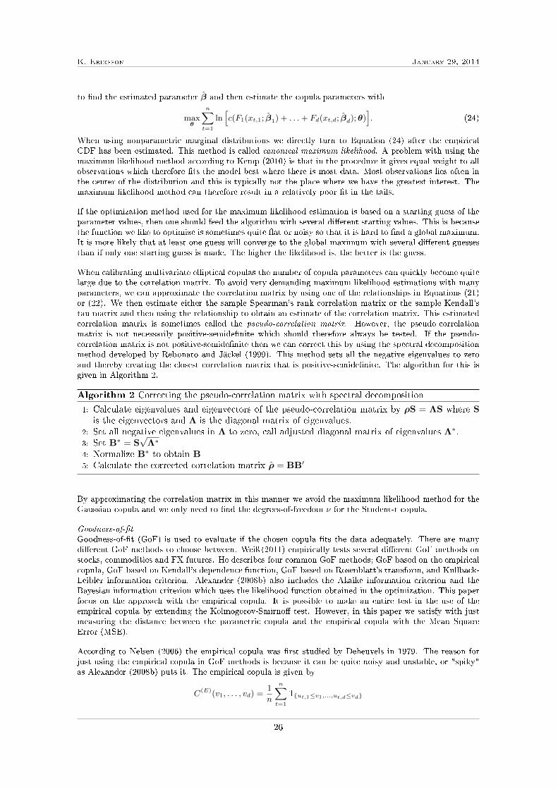
K. Eriksson January 29, 2014
to nd the estimated parameter β and then estimate the copula parameters with
maxθ
n∑t=1
ln[c(F1(xt,1; β1) + . . .+ Fd(xt,d; βd);θ)
]. (24)
When using nonparametric marginal distributions we directly turn to Equation (24) after the empiricalCDF has been estimated. This method is called canonical maximum likelihood. A problem with using themaximum likelihood method according to Kemp (2010) is that in the procedure it gives equal weight to allobservations which therefore ts the model best where there is most data. Most observations lies often inthe center of the distribution and this is typically not the place where we have the greatest interest. Themaximum likelihood method can therefore result in a relatively poor t in the tails.
If the optimization method used for the maximum likelihood estimation is based on a starting guess of theparameter values, then one should feed the algorithm with several dierent starting values. This is becausethe function we like to optimize is sometimes quite at or noisy so that it is hard to nd a global maximum.It is more likely that at least one guess will converge to the global maximum with several dierent guessesthan if only one starting guess is made. The higher the likelihood is, the better is the guess.
When calibrating multivariate elliptical copulas the number of copula parameters can quickly become quitelarge due to the correlation matrix. To avoid very demanding maximum likelihood estimations with manyparameters, we can approximate the correlation matrix by using one of the relationships in Equations (21)or (22). We then estimate either the sample Spearman's rank correlation matrix or the sample Kendall'stau matrix and then using the relationship to obtain an estimate of the correlation matrix. This estimatedcorrelation matrix is sometimes called the pseudo-correlation matrix. However, the pseudo-correlationmatrix is not necessarily positive-semidenite which should therefore always be tested. If the pseudo-correlation matrix is not positive-semidenite then we can correct this by using the spectral decompositionmethod developed by Rebonato and Jäckel (1999). This method sets all the negative eigenvalues to zeroand thereby creating the closest correlation matrix that is positive-semidenite. The algorithm for this isgiven in Algorithm 2.
Algorithm 2 Correcting the pseudo-correlation matrix with spectral decomposition
1: Calculate eigenvalues and eigenvectors of the pseudo-correlation matrix by ρS = ΛS where Sis the eigenvectors and Λ is the diagonal matrix of eigenvalues.
2: Set all negative eigenvalues in Λ to zero, call adjusted diagonal matrix of eigenvalues Λ∗.3: Set B∗ = S
√Λ∗
4: Normalize B∗ to obtain B5: Calculate the corrected correlation matrix ρ = BB′
By approximating the correlation matrix in this manner we avoid the maximum likelihood method for theGaussian copula and we only need to nd the degrees-of-freedom ν for the Student-t copula.
Goodness-of-tGoodness-of-t (GoF) is used to evaluate if the chosen copula ts the data adequately. There are manydierent GoF methods to choose between. Weiÿ (2011) empirically tests several dierent GoF methods onstocks, commodities and FX futures. He describes four common GoF methods; GoF based on the empiricalcopula, GoF based on Kendall's dependence function, GoF based on Rosenblatt's transform, and Kullback-Leibler information criterion. Alexander (2008b) also includes the Akaike information criterion and theBayesian information criterion which uses the likelihood function obtained in the optimization. This paperfocus on the approach with the empirical copula. It is possible to make an entire test in the use of theempirical copula by extending the Kolmogorov-Smirno test. However, in this paper we satisfy with justmeasuring the distance between the parametric copula and the empirical copula with the Mean SquareError (MSE).
According to Nelsen (2006) the empirical copula was rst studied by Deheuvels in 1979. The reason forjust using the empirical copula in GoF methods is because it can be quite noisy and unstable, or "spiky"as Alexander (2008b) puts it. The empirical copula is given by
C(E)(v1, . . . , vd) =1
n
n∑t=1
1ut,1≤v1,...,ut,d≤vd
26

K. Eriksson January 29, 2014
where 1· is the indicator function and (v1, . . . , vd) ∈ [0, 1]d.
The empirical copula is then compared with the parametric copula by using the MSE
MSE =1
n
n∑t=1
(C
(E)t − Ct
)2
.
A smaller MSE implies a better t between the empirical and parametric copula.
Simulation with copulasThere are many ways in how to simulate from copulas but three popular ones are; simulation with condi-tional copulas, simulation with elliptical copulas and Marshall and Olkin algorithm. An example of howsimulations from the Gaussian, Student-t, Clayton and Gumbel copulas can look like are presented in Figure12.
Figure 12: Simulations from the Gaussian, Student-t, Clayton and Gumbel copula.
The simulation with conditional copulas is the most general of the three but it can for certain copulas bedicult to nd the conditional copulas or the inverse of the conditional copula. Sometimes we must turnto numerical procedures to nd these which then make the approach of simulation with conditional copulasquite demanding. The reason why the conditional algorithm is the most general of the three is because itcan simulate from any copula, given that we can nd the conditional copula and its inverse. The algorithmcan be found in Cherubini et al. (2004), Nelsen (2006) and Alexander (2008b).
Algorithm 3 Simulation with conditional copulas
1: Generate the variates from an independent uniform distribution (u1, . . . , ud) ∼ U (0, 1)2: Set u∗1 = u1 and use the inverse of the conditional copula u∗2 = C−12|1(u2|u∗1)
3: for i = 3 to d do4: Calculate u∗i = C−1i|1,...,i−1(ui|u∗1, . . . , u∗i−1)
5: end for
6: Use the inverse marginal distributions to obtain (x1, . . . , xd) = (F−11 (u∗1), . . . , F−1d (u∗d))
An easier algorithm based on Cholesky decomposition is available if we would like to simulate from ellipticalcopulas. This is also a popular algorithm and can be found in Cherubini et al. (2004), McNeil et al. (2005)and Alexander (2008b). See Algorithm 4 for how to simulate from elliptical copulas.
27

K. Eriksson January 29, 2014
Algorithm 4 Simulation with elliptical copulas
1: Let Gi(xi) =
Φ(xi) if simulating from Gaussian copulatv(xi) if simulating from Student-t copula
2: Generate the variates from an independent uniform distribution (u1, . . . , ud) ∼ U (0, 1)3: Set xi = G−1i (ui).4: Perform a Cholesky decomposition of the covariance matrix Σ = LL′.5: Calculate x∗ = Lx6: Obtain the simulated uniform generates (u∗1, . . . , u
∗d) = (G1(x∗1), . . . , Gd(x
∗d))
7: Use the inverse marginal distributions to obtain (x1, . . . , xd) = (F−11 (u∗1), . . . , F−1d (u∗d))
The last algorithm, the Marshall and Olkin algorithm, can be used to simulate from certain Archimedeancopulas. The algorithm requires some deep theoretical foundations and the reader is recommended toconsult this theory in McNeil et al. (2005). A description of how to simulate from the Clayton and Gumbelcopula is presented in Algorithm 5.
Algorithm 5 Marshall and Olkin algorithm
1: Generate a variate V , for the Clayton copula the variate is generated from the gamma distri-bution V ∼ Ga(1/θ, 1) and for the Gumbel copula the variate is generated from the positivestable distribution V ∼ St(1/θ, 1, γ, 0) where γ = (cos(π/(2θ)))θ.
2: Generate variates from an independent uniform distribution (u1, . . . , ud) ∼ U (0, 1).3: Calculate (u∗1, . . . , u
∗d) = (G(− ln(u1)/V ), . . . , G(− ln(ud)/V )). For the Clayton copula G(t) =
(1 + t)−1/θ and for the Gumbel copula G(t) = exp(−t1/θ)4: Use the inverse marginal distributions to obtain (x1, . . . , xd) = (F−11 (u∗1), . . . , F−1d (u∗d))
2.2.4 Stochastic models
Up until now we have assumed that the random variables are i.i.d. processes. This assumption is veryharsh but there are ways to soften this assumption. In nance the returns are often assumed to be weaklystationary (Tsay, 2010). McNeil et al. (2005) lists a number of stylized facts about nancial time series,here is a short summary:
• Return series are heavy-tailed.
• Extreme returns tends to come in clusters (volatility clustering).
• Extreme returns also tends to coincide with extreme returns in other series.
• Volatility varies over time.
• Leverage eect (volatility tends to increase more after a negative return).
• Correlations varies over time.
To make the models a bit more exible, an exponential moving average could be applied to the time series.This would then give more weights to the most recent observations. However, we would still assume thatthe random variables are i.i.d. processes. To model the volatility we could instead use the GeneralizedAutoregressive Conditional Heteroscedasticity (GARCH) model. The ARCH model was rst introduced byEngle (1982) and generalized by Bollerslev (1986). The GARCH model is given by
σ2t = ω + αε2t−1 + βσ2
t−1
where ω, α, β are parameters, ε2 is the return innovations and σ2 is the conditional variance. The GARCHmodel is a purely symmetric model so it cannot handle the asymmetric behaviour of the leverage eect.Another popular model that can account for the leverage eect is the Exponential GARCH (EGARCH) byNelson (1991)
ln(σ2t ) = ω + θzt−1 + γ(|zt−1| − E[|zt−1|]) + β ln(σ2
t−1)
where ω, θ, γ, β are parameters and z is an i.i.d. random variable with mean zero and variance one, relatedto the return innovations by z = ε/σ. See Tsay (2010) for more information about these models and many
28

K. Eriksson January 29, 2014
other GARCH models. To handle that the correlation varies over time we need to turn to multivariateGARCH models. The main focus of this paper is however to study features of copulas and not to createthe "perfect" model. We will therefore not use the GARCH models but it is important to know that it ispossible to turn to them if needed. The interested reader can nd an introduction to multivariate GARCHmodels in McNeil et al. (2005) and Alexander (2008b).
2.3 Risk measures
Risk is the uncertainty of a potential deviation from an expected result. It is not a matter of the past,but the future uncertainty. There are a wide variety of risk measures. Standard deviation was used as arisk measure already in the popular mean-variance portfolio theory from 1952 by Harry Markowitz. Recallthe formal denition of a random variable X given in the section about probability theory. The standarddeviation is dened as
σ(X) = ‖X − E[X]‖2where ‖·‖2 is the 2-norm. Another closely related and popular risk measure is the mean absolute deviation(MAD)
MAD(X) = ‖X − E[X]‖1 .However, both standard deviation and MAD are symmetric which means that they incorporates both theupside and downside deviations. This is not a satisfactory property for a risk measure in nance sincewe typically have an asymmetry between the upside and downside (we often observe more spectacularmovements on the downside). According to Krokhmal et al. (2011) even Markowitz suggested the use of amore appropriate risk measure than the standard deviation and recommended the use of semivariance
σ2−(X) = ‖(X − E[X])−‖22
where (X − E[X])− is the observations on the downside. The semivariance is therefore a downside riskmeasure. Rockafellar et al. (2006) introduced an entire class of deviation measures where the standarddeviation, MAD and the square root of the semivariance are all included. From now on we will only focuson downside risk measures.
In the pioneering work by Artzner et al. (1999) a number of axioms are used to dene a "good risk measure",or as the authors name it, a coherent risk measure. They suggest that a risk measure should measure howfar away a certain position is from being accepted by some "higher power" like a regulator or an investmentmanager. This means that a benchmark level is set from where the deviation from the expected resultis viewed as a risk (for example we could set the benchmark at the same level as what we bought theinvestment for and therefore consider this level to be what is acceptable, any possible losses would then beunacceptable). Now suppose that there is a reference instrument that if added to the portfolio it wouldmake the position more acceptable (this reference instrument could be cash, we can hold cash to cover ourlosses). Then Artzner et al. (1999) suggest that a good candidate for a risk measure is the current cost ofthese reference instruments that would make the position acceptable.
A risk measure is dened in the following denition.
Denition 2.12. Consider the set of all risks G, then a risk measure δ is the mapping δ : G → R.
This means that a risk measure is the function that gives a scalar value on R based on the set of all risks.
2.3.1 Axioms
To dene what is a good risk measure Artzner et al. (1999) used an axiomatic approach. Consider a strictlypositive return r for the reference instrument and an initial amount α, then a coherent risk measures satisesthe following axioms:
Axiom M: (Monotonicity) δ(X2) ≤ δ(X1) for all X1, X2 ∈ G where X2 ≥ X1.
Axiom T: (Translation invariance) δ(X + αr) = δ(X)− α for all X ∈ G and all real numbers α.
Axiom PH: (Positive homogeneity) δ(λX) = λδ(X) for all X ∈ G and λ ≥ 0.
Axiom S: (Subadditivity) δ(X1 +X2) ≤ δ(X1) + δ(X2) for all X1, X2 ∈ G.
29

K. Eriksson January 29, 2014
An economical interpretation of the axioms would then be as follows. Axiom M means that if we have twoassets, and asset 1 always takes on more negative values than asset 2, then the risk for asset 1 should behigher. Axiom T tells us that if we increase the amount of the reference instrument then we will decreasethe risk and vice versa. This is logical; if we only hold cash then there would be no risk. Axiom PH relatesto the size of the portfolio, if the size is greater then so is the risk ("double the bet, doubles the risk").Axiom S concerns diversication, a risk measure that fullls S incorporates that it is possible to diversifya portfolio. Axiom PH and S together ensures that when increasing the size of the original portfolio thendiversication is not possible.
Any risk measure that fullls Axiom M and T is called aMonetary risk measure (Föllmer and Schied, 2008).It is easy to see from Axiom M that the standard deviation and MAD are not Monetary risk measures sincethey only measure how much X deviates from its mean. A monetary risk measure that fullls the followingaxiom
Axiom C: (Convexity) δ(λX1 + (1− λ)X2) ≤ λδ(X1) + (1− λ)δ(X2) for 0 ≤ λ ≤ 1 and all X1, X2 ∈ G.
is called a Convex risk measure (Föllmer and Schied, 2008). The convex risk measures was developedseparately by (Föllmer and Schied, 2002) and (Frittelli and Gianin, 2002). It weakens the axioms PH andS but gives a more direct meaning to diversication. See (Föllmer and Schied, 2008) for a closer discussionabout convex risk measures.
In practice we would also want the following axioms:
Axiom L: (Law-invariance) δ(X1) = δ(X2) if their CDFs FX1 = FX1 for all X1, X2 ∈ G.Axiom CA: (Comonotonic additivity) δ(X1 +X2) = δ(X1) + δ(X2) for all comonotonic r.v. X1, X2 ∈ G.
Axiom L is straightforward; if the assets have equivalent distributions then the risk measures should yieldthe same results. Axiom CA means that if two assets are comonotonic then diversication is not possible.
2.3.2 Value-at-Risk
Value-at-Risk (VaR) has become one of the most popular ways to measure risk in nance. It is howevernot a perfect measure. Value-at-Risk is the minimum loss we would expect for a given probability over acertain period (risk horizon). It is basically the α-quantile of the distribution of X.
V aRα(X) = −infx ∈ R|P (X ≤ x) > α
Value-at-Risk is illustrated in Figure 13. The reason for its popularity is because it is easy to calculate andevaluate, and it is simple to understand. But there are many drawbacks. Artzner et al. (1999) show thatValue-at-Risk is not a coherent risk measure in general because it fails to full Axiom S, see the classicalExample 2.5. This is a big problem since it could in fact discourage diversication. Value-at-Risk is onlycoherent in the case of a joint normal distribution.
Example 2.5. Consider two defaultable zero coupon bonds with maturity in 1 year. Assume that thebonds have two dierent issuers and that each bond has a 4% probability of default that is independent ofthe other. In the case of default the recovery rate is 30%. Assume also that the yields for the bonds arezero. Calculate the 95% Value-at-Risk for both bonds separately and for the combined portfolio with equalweight on each bond.
The solution is trivial for calculating Value-at-Risk of the bonds separately; because the probability ofdefault is only 4% which means that it is further out in the tail than the chosen quantile of Value-at-Risk, so V aR1 = 0 and V aR2 = 0. For the portfolio the probability that one of the bonds will default is2 · 0.04 · 0.96 ≈ 0.077. This means that the Value-at-Risk for the portfolio is 35%.
This example illustrates another problem with Value-at-Risk, since it relies only on a quantile of thedistribution it gives no information about what is going on further out in the tail. Possibly huge lossescould be obtained if Value-at-Risk is exceeded. Value-at-Risk is also very easy to manipulate because itonly uses the quantile. We could create a portfolio with a small Value-at-Risk but with enormous downsideif Value-at-Risk is exceeded.
30

K. Eriksson January 29, 2014
2.3.3 Expected shortfall
Expected shortfall (ES) is a coherent risk measure and addresses some of the problems with Value-at-Risk.It measures the average loss given that Value-at-Risk has been exceeded. This makes it not as easy tomanipulate as Value-at-Risk and it does gives a "how much could be lost" output. See Figure 13 for anillustration of Expected shortfall. Expected shortfall is related to many dierent names of risk measures.The name and the development of the Expected shortfall were due to Acerbi et al. (2001). Related to theExpected shortfall is the Conditional Value-at-Risk (CVaR) by Rockafellar and Uryasev (2002). In Artzneret al. (1999) the Tail conditional expectation (TCE) and the Worst conditional expectation (WCE) canbe found. The TCE and WCE are predecessors to ES and CVaR. Acerbi and Tasche (2002) give a greatsummary of the dierences between ES, CVaR, TCE and WCE, and prove that ES and CVaR are equivalent.Expected shortfall is dened as
ESα(X) = −α−1 (E[X]1X≤xα + xα(α− P (X ≤ xα)))
where xα is the α-quantile of the distribution. Acerbi (2002) derived the following representation of Expectedshortfall
ESα(X) =1
α
∫ α
0
V aRλdλ
which gives a more direct view of what Expected shortfall really is.
The main problem with Expected shortfall compared to Value-at-Risk is that we need a huge amount of datato be able to backtest Expected shortfall accurately as we will see in Section 2.5 Backtesting. Furthermore,Balbás et al. (2009) gives the following example of a problem with Expected shortfall.
Example 2.6. Consider two assets A and B, with probability of losses given in Table 2.
Table 2: Losses and probability of the losses for asset A and B.
Loss P(A) P(B)
0 0.6 09 0 0.610 0.4 0.4
Then the 95% Expected shortfall for the two assets are ESA = 10 and ESB = 10 even though we wouldconsider asset B more risky than asset A.
Figure 13: An illustration of Value-at-Risk and Expected shortfall.
31

K. Eriksson January 29, 2014
2.3.4 Spectral risk measures
Spectral risk measures were developed by Acerbi (2002) and is an entire class of risk measures whereExpected shortfall is a special case. Adam et al. (2008) states that the spectral risk measures fullls boththe axioms of coherence and Axiom L and CA. The spectral risk measures tries to link the risk measurewith a utility function. The user can then create their own coherent risk measure. A spectral risk measurein general is however not as easy to describe as Value-at-Risk and Expected shortfall. The spectral riskmeasures are given by
Mφ(X) = −∫ 1
0
F−1X (p)φ(p)dp
where φ(·) is the risk-aversion function that satises
1. Non-negativity: φs ≥ 0
2. Normalization:∑Ss=1 φs = 1
3. Monotonicity: φs is nondecreasing.
For Expected shortfall the risk-aversion function is φ(p) = 10≤p≤α/α.
2.3.5 Distortion risk measures
Distortion risk measures were introduced by Wang (1996) and Wang et al. (1997). Adam et al. (2008)states that the distortion risk measures fullls axioms M, T, PH, L, CA. Distortion risk measures are aninteresting class of risk measure because almost all risk measures that can be written in the form of anintegral can be obtained. The distortion risk measures are calculated by using the Choquet integral
δg(X) = −∫ 0
−∞(1− g(1− FX(x)))dx+
∫ ∞0
g(1− FX(x))dx
where g(·) is the distortion function. For Value-at-Risk the distortion function is given by
gV aR(u) =
0, if 0 ≤ u < 1− α1, if 1− α ≤ u ≤ 1
and for Expected shortfall
gES(u) =
u
1−α , if 0 ≤ u < 1− α1, if 1− α ≤ u ≤ 1
The problem observed for Expected shortfall in Example 2.6 can be avoided according to Balbás et al.(2009) by using complete and adapted distortion risk measures (see Balbás et al. (2009) for the denition).One such risk measure is the Wang's transform that was developed by Wang (2000) and has the followingdistortion function
gWT (u) = Φ(Φ−1(u) + κ)
where Φ is the standard normal distribution and κ is a parameter that reects systemtic risk.
2.4 Estimating risk
If nancial time series would actually behave as the dened random variables in the probability section withi.i.d. processes and the true distribution for the future was known, then the risk measures above would giveexactly what they promise to give, no more nor less. However, the world is not so easy. We therefore needto know that the models we use are simplied depictions of the real world. Sometimes are these models toosimplistic and will therefore produce results that make no sense. Keep in mind that the future is not easyto predict.
Since the distribution of the future is not known we have to estimate it. This can be done in various ways;by a parametric, nonparametric or semiparametric approach. Each are described shortly below.
In practice we have limited computer power. This means that it might not be possible to estimate the riskdirectly of a huge portfolio by considering each asset in it. There are ways to reduce the dimensions byfor example using factor analysis, principal component analysis (PCA) or Taylor approximations. Thesemethods tries to nd a way to describe the behaviour of the portfolio by applying certain risk factors thatwe believe can capture the behaviour. Using some sort of dimension reduction technique is called riskmapping. See Alexander (2008b and 2008c) for an introduction to risk mapping.
32

K. Eriksson January 29, 2014
2.4.1 The parametric approach
The parametric approach can be used when we assume that the future distribution can be described bysome simple parametric distributions (elliptical). The advantage with this method is that we can obtainan analytical formula for the risk measures. For example, for Value-at-Risk with an assumed joint normaldistribution we have the analytical formula
V aRα(x) = Φ−1(1− α)√
wΣw′ −w′µ
where w is the portfolio weights, µ is the expected return vector and Σ is the covariance matrix. Thismakes this method very appealing since we can easily obtain the risk estimates. However, if the futuredistribution is clearly not close to the assumed parametric distribution then this method performs verypoorly.
2.4.2 The nonparametric approach
The nonparametric approach which is most commonly known as historical simulation does not make anyparametrical assumptions and therefore relies completely on the historical data of the portfolio. Thisimplicates that a suciently large historical sample must be used to get a reliable model. The numberof observations in the tails might otherwise be too few. This is a serious problem since the risk measureswe want to apply are based in the tails of the distribution. With a large historical sample comes thepossibility that the market dynamics has changed between the most recent observations and the mosthistorical observations. The model can be extended to more sophisticated models like the Weighted historicalsimulations or Filtered historical simulations.
2.4.3 The semiparametric approach
The semiparametric approach is a combination between the parametric and nonparametric approaches. Itoften involves Monte Carlo methods (but not necessary). See the excellent book by Glasserman (2003) fordetails about Monte Carlo methods. There are many dierent kinds of semiparametric models, for examplesmoothing procedures of the historical data or Cornish-Fisher approximation. This paper uses ExtremeValue Theory (EVT) to estimate the lower tails of the marginal distributions. EVT is a way to modelextreme events. It is an entire science in itself so this paper is just going to scratch the surface of thistheory. The discussion that follows is based on the books by Beirlant et al. (2004), McNeil et al. (2005)and Kemp (2010).
A motivation for the use of EVT is; what if we want to calculate the probability of a possible, but veryunlikely event in the tail of a sample, where the sample probability is zero? In ordinary statistics we areusually concerned about the averages and higher moments, but what if the rst or second moment is notnite? The central limit theorem then breaks down. Hence, we need to study extremes in a special way.This is where EVT comes into the picture.
EVT tries in a statistical way to handle extreme events by considering the tails of a distribution and itscharacteristics. The procedure usually consists of tting a distribution to the observations in the tails andfrom the t extrapolates even more extreme events that are not already observed.
But what are extreme events? Kemp (2010) answers this question in the following way "Events are only'extreme' when measured against something else". An example of this could be; Is drinking 30 cups of coeein a day extremely much? - Perhaps yes, if we usually drink 5 cups/day. - Perhaps no, if we usually drink 30cups/day. In EVT two common ways to dene the extreme events of a distribution are the Maxima seriesapproach and the Point over threshold (POT) method. Both these methods are illustrated in Figure 14.With the maxima series we divide the historical sample into smaller subsamples and nds the max in each ofthe subsamples. This method therefore throws away many extreme events (remember that extreme returnstends to come in clusters) and keep less extreme events. The method often used nowadays is therefore thePOT method. In POT we set a certain threshold level Θ for which all observations above (below, if workingwith the lower tail) is considered extreme. How to choose the threshold level is not trivial but around 10%is a good rule of thumb.
Certain distributions of extremes obtained by the POT method converge to the generalized Pareto distri-bution. Which distributions that converges are described in the Pickands-Balkema-de Hann theorem, see
33

K. Eriksson January 29, 2014
Figure 14: An illustration of the maxima series (left) and the point over threshold (right).
McNeil et al. (2005) for details. The generalized Pareto distribution is given by
G(x; ξ, β) =
1− (1 + ξx/β)−1/ξ, ξ 6= 01− exp(−x/β), ξ = 0
where ξ is the shape parameter and β is the scale parameter. When ξ ≥ 0 then β > 0 and x > 0, and whenξ < 0 then 0 ≤ x ≤ −β/ξ.
The parameters can be estimated with for example the maximum likelihood method. However, we canestimate ξ without making any parametric assumption by using the Hill estimator. To use the Hill estimator;start by ordering the data of X, x(o)
1 < . . . < x(o)n and then nd the x(o)
i that corresponds to the thresholdlevel. The threshold level x(o) is at the position k so x(o)
k is the threshold x(o). Then the Hill estimator isgiven by
ξ(H) =1
k
k∑i=1
ln
(x
(o)i
x(o)k
). (25)
To obtain the estimated tail distribution by only using ξ(H) we can follow the procedure that is describedin McNeil et al. (2005). In this procedure an approximated generalized Pareto distribution is used
Ftail(x) = 1− k
n
(x
x(o)k
)−1/ξ(H)
. (26)
By using this method we avoid the use of a maximum likelihood method that would be more computationaldemanding. However, this method is not as accurate.
Kemp (2010) lists a number of issues with using EVT; extrapolation is not as good as interpolation and wedo not know how the tails actually looks like after the worst observation. It is not necessary that the sampledistribution converges to the generalized Pareto distribution. The theory relies heavily on the assumptionof stationary processes since the extreme observations clusters often are distant from each other.
2.5 Backtesting
Backtesting a risk measure in a general way is not easy because they all measure somewhat dierent things.For example, the procedure to backtest Value-at-Risk is not the same as backtesting Expected shortfall.This section outlines only simple backtesting procedures for Value-at-Risk and Expected shortfall. Both thebacktesting procedure for Value-at-Risk and the backtesting procedure for Expected shortfall can be foundin Alexander (2008d). The general part is that Value-at-Risk and Expected shortfall must be estimatedover a backtesting sample. The risk horizon in both risk measures is one day in this paper so the Value-at-Risk and Expected shortfall must be estimated daily (with longer risk horizons the backtesting procedure
34

K. Eriksson January 29, 2014
involves non-overlapping windows). The sample must be quite large, especially for Expected shortfall sothat we obtain a distribution of losses that has exceeded Value-at-Risk. The estimated risk measures arecompared against the observed returns at the end of the risk horizon. In the case of one day, then −V aRtand −ESt are compared with the return Xt+1.
Backtest Value-at-RiskThe backtesting of Value-at-Risk rely on the assumption that the returns can be represented by a Bernoulliprocess. The Bernoulli distribution takes two values, either "success" or "failure". The sample of n returnswith chosen signicance level α for the Value-at-Risk model can for the Bernoulli distribution be formulatedby the following 95% condence interval
(nα− 1.96√nα(1− α), nα+ 1.96
√nα(1− α)).
Then it is just a matter of comparing the number of exceedances of the estimated Value-at-Risk with theabove condence interval.
Backtest Expected shortfallThe following method was developed by McNeil and Frey (2000) and builds on the standardized exceedanceresiduals
ε∗t+1 =
−Xt+1−ESt
σt, Xt+1 < −V aRt
0 Otherwise
where σt is the estimated standard deviation of the returns. Let ε = εt+1|Xt+1 < −V aRt be theexceedance residuals that only contains the observations of losses over the Value-at-Risk and set nε to bethe amount of such occurrences. The test statistic is
Q =ε
σ(ε)/√nε
where ε is the mean and σ(ε) the standard deviation of ε. A bootstrap procedure can be used to nd thedistribution of Q. Let (Q∗1, . . . , Q
∗B) be B bootstrap samples from Q, then the p-value can be calculated
p =1
1 +B
(1 +
B∑i=1
1Q∗i>Q
).
2.6 Stress testing
Stress testing is a way to investigate how the risk models work under stressed scenarios. The scenarios canbe based on historical scenarios or by hypothetical scenarios. The historical scenarios are based on historicalsamples and are therefore bound to only consider what has occurred. The question could for example be,how much could we lose if the nancial crisis of 2008 re-occurred. With hypothetical scenarios on the otherhand, allows us model our own believes in a more exible way. What if there is a shift in a certain riskfactor or what if the correlation increases. This kind of model can be obtained by Monte Carlo methods.The copula models should serve as a good tool to create hypothetical scenarios.
Stress testing are more concerned with the word "potential loss" rather than "how often do we lose". Thehypothetical scenarios are also a way to test the risk model since we can create many dierent kinds ofscenarios, instead of just relying on one historical path. It is possible to create the "the perfect storm" andsee if/when the risk models breaks down.
The readers who are searching for more information about stress testing can nd it in Alexander (2008d)and Kemp (2010).
35

K. Eriksson January 29, 2014
3 Method
This section describes the method used for the empirical part of this study. First by providing more detailsabout the implementation and then a brief summary of the data used in this study is given.
3.1 Implementation
The implementation focuses on testing the copula models in the framework of risk calculations and stresstesting. This empirical study is divided into three steps:
1. Backtesting of Value-at-Risk and Expected shortfall with copula models and historical simulation.
2. Copula parameters under stressed and calm market periods.
3. Stess testing.
Step 1 focus on comparing the copula models with the historical simulation by using the risk estimatesof Value-at-Risk and Expected Shortfall. We can evaluate Value-at-Risk and Expected shortfall with thebacktesting procedure described in the section about backtesting. Hence, the results obtained for thebacktesting of the risk measures can therefore be used to evaluate how good the copula models and thehistorical simulation was in the framework of these risk measures during the specied backtesting timeperiod.
Step 2 considers only the parameters of the copula models and the parameters for the marginal distributions.It is interesting to investigate how the parameters changes in dierent market periods because it would giveus the knowledge of how the copula models can be stressed so that they behave as under historical crises.Goodness-of-t is also used in this step to see how well the copulas t the data.
Step 3 backtests the Value-at-Risk and Expected shortfall with stressed parameters in the copula modelsto investigate how the stressed risk measures would have behaved during the backtesting time period.
The copula models considered are
• Gaussian copula
• Student-t copula
• Clayton copula
and the marginal distributions are based on
• Empirical CDF
• Empirical CDF with Extreme Value Theory in the lower tail.
This means that six copula models are implemented. The Gaussian and Student-t copulas are calibratedwith the pseudo-correlation matrix based on Kendall's tau and the parameter ν in the Student-t copulais calibrated by using maximum likelihood in Equation (24). The simulation algorithm for the Gaussianand Student-t copulas are Algorithm 4. The Clayton copula is calibrated with the same procedure as theStudent-t copula parameter ν and simulations from the Clayton copula is made by using Algorithm 5. Thenumber of simulations is set to 10000, this is really not enough but it suces for illustrating the use ofcopula models (Alexander, 2008b).
The marginal distributions are constructed by using Equation (23). For the Empirical CDF with EVT lowertail, the empirical lower tail is changed for the estimated EVT tail. The EVT tail is based on the Pointover Threshold method with threshold level at 10%. The Hill estimator is used to t the approximatedgeneralized Pareto distribution, see Equation (25) and (26).
The Value-at-Risk and Expected shortfall are evaluated at the signicance level of 99% with a risk horizonof one day. According to Alexander (2008d) the 99% Value-at-Risk for historical simulation should be basedon at least 2000 observations. Therefore, the sample size for the historical simulation is set to 2000. The
36

K. Eriksson January 29, 2014
copula models do not need such a big sample size and are therefore only based on a sample size of 500. Therisk measures are estimated on the portfolio with equal weights of each asset.
Figure 15 illustrate a ow chart of Step 1 in the implementation. Step 2 and 3 are built in a similar way.
Figure 15: A ow chart over the implementation of Step 1.
3.2 Data
The data this paper uses consists of ve dierent large indices for the time period 1984-01-03 to 2013-11-21.The ve indices are:
• Dow Jones Industrial Average: The current owner of the Dow Jones indices is S&P Dow JonesIndices. According to S&P Dow Jones Indices: Averages (2014) the Dow Jones Industrial Averagewas introduced in 1896-05-26 by Charles H. Dow. In the very beginning the index consisted of 12stocks, mostly in railroads. It was not until 1928 that the index was expanded to 30 stocks. TodayDow Jones Industrial Average consists of 30 stocks of large companies based in U.S. About two-thirdsof the stocks are manufacturing companies and the rest is in nancial services, entertainment and IT.
• S&P 500 : S&P 500 is a U.S. stock index developed and owned by S&P Dow Jones Indices. It includes
37

K. Eriksson January 29, 2014
500 of the largest U.S. companies in the leading industries and cover approximately 80% of the U.S.stock market capitalization according to S&P Dow Jones Indices: S&P 500 (2014).
• NYSE Composite: NYSE Composite is a stock index which includes all common stocks on the NewYork Stock Exchange. The index is owned by NYSE Euronext and in 2004 it included over 2000 U.S.and non-U.S. stocks according to NYSE Euronext (2014).
• NASDAQ Composite: A stock index that includes all common stocks listed on NASDAQ and ownedby NASDAQ OMX. According to NASDAQ OMX: COMP (2014) the index began in 1971-02-05 andtoday it includes over 2500 companies.
• PHLX Gold/Silver sector : A sector index of companies in the gold and silver sector traded on thePhiladelphia Stock Exchange which is now owned by NASDAQ OMX. The index is also owned byNASDAQ OMX and according to NASDAQ OMX: XAU (2014), the index was introduced in 1979-01-19 with a base value of $100.
The data for Dow Jones was obtained from Federal Reserve Bank of St. Louis (2014) and the data for therest of the indices were obtained from Yahoo Finance (2014). See Appendix A for a visualization of theprice and return for the ve indices.
To investigate the parameters of the copula models under stressed and calm market periods the data hasbeen divided up in stressed and calm periods as in Table 3. It is not trivial to determine when the market isin a "stressed" or "calm" period. This paper uses the methodology of visual inspection of the return series(looking at how volatile the returns are) and to some degree the price series in Appendix A, together witha short historical research about nancial crises in the sample period. Most of the history about nancialcrises are gathered from the book by Ferguson (2009) and his documentary.
During the period of 1982-1987 the U.S. stocks was in general in a nancial rally with climbing prices. Itwas not until the Black Monday in October 1987 (1987-10-19) when the sudden crash came. It was thesingle largest fall in the price of one day in the history of Dow Jones Industrial Average (approx. 22%). Theturmoil after the Black Monday lasted for a short while but had its impact on the traders. After the crashthe commonly known volatility smiles became present in the implied volatility of options. During a shortperiod of more calm markets the next turmoil started in the late 1980s (1989) and the beginning of the1990s with the U.S. saving and loaning crisis. During this period the Japanese asset bubble had also burst.The recession observed in the beginning of the 1990s was followed by another rally in the middle of the1990s which is commonly referred to as the Dot-com bubble. The beginning of the end of this rally startedin 1997 with the Asian nancial crisis and followed by the default of Russia in 1998-08-17. The default ofRussia was the starting signal of the end of the well-known hedge fund Long-Term Capital Managementwhich collapsed in a spectacular manner. During this period the great depression in Argentine was alsostarted. In the beginning of 2000 the Dot-com bubble burst and it was not until the end of 2002 that thestock indices started to increase in value again. This was the start of an additional tremendous increasein the price for some years until the nancial crisis of 2007-2008 started. This crisis is referred to as theworst crisis since the great depression in the 1930s. The nancial crisis of 2007-2008 was followed by theEuropean sovereign debt crisis that started in 2010. It is not easy to nd "calm" periods in the chosensample period but the volatility of the returns seems lower when the prices are going up and therefore arethese periods considered as "calm" while the spectacular crashes are dened as "stressed" periods.
Table 3: Dates for stressed and calm market periods.
Stressed Calm
Period Dates Period Dates
87.5-88.5 1987-07-01 to 1988-06-30 84-87.5 1984-01-03 to 1987-06-3089.5-92.5 1989-07-03 to 1992-06-30 88.5-89.5 1988-07-01 to 1989-06-3097-03.5 1997-01-02 to 2003-06-30 92.5-97 1992-07-01 to 1996-12-3107-10 2007-01-03 to 2009-12-31 03.5-07 2003-07-01 to 2006-12-2910-12 2010-01-04 to 2011-12-30 12-End 2012-01-03 to 2013-11-21
38

K. Eriksson January 29, 2014
4 Results
The results presented in this section comes from the three steps described in the section about implementa-tion. The rst step is to backtest the dierent copula models by using Value-at-Risk and Expected shortfalland compare it with historical simulation. The second step is to further investigate how the parameters inthe copulas change under stressed and calm market periods. The third step is to apply stressed parametersto the copula models and see how Value-at-Risk and Expected shortfall would have performed under sucha stressed model.
Step 1: Backtesting of Value-at-Risk and Expected shortfall with copula models and historical simulation.The illustration of the backtesting can be found in Appendix B. In Table 4 the backtesting result of theValue-at-Risk are presented. The number of exceedances is the measure of how well the model has behaved,where on a 95% condence level the number of exceedances should be on the interval (41, 69). This indicatesthat all models but the Clayton copula model with EVT tail and the historical simulation approach workswell. The Clayton copula model with EVT tail is indicated to be too conservative since the number ofexceedances is less than the interval, while the historical simulation indicates to underestimate the risk.
Table 4: Number of exceedances in the backtesting of 99% Value-at-Risk over the period 1991-11-22 to 2013-11-21. The 95% condence interval for the number of exceedances is (41, 69). The copula models uses bothempirical marginal distributions and marginal distributions based on Extreme value theory.
Backtesting Value-at-Risk
Type Empirical Extreme Value
Gaussian copula 63 53Student-t copula 68 59Clayton copula 68 33
Historical simulation 83
The Expected shortfall is backtested with another technique than by counting number of exceedances (seesection backtesting). Here we obtain p-values that test the null hypothesis that the estimated Expectedshortfall is equal or more conservative against the alternative hypothesis that the estimated Expectedshortfall underestimates the risk. In Table 5 we see that on a 5% signicance level the null hypothesis arerejected for the copula models with empirical marginal distributions but are not rejected for the copulamodels based on marginal distributions with EVT tails and the historical simulation approach.
Table 5: The p-values of the backtesting of 99% Expected shortfall over the period 1991-11-22 to 2013-11-21.The copula models uses both empirical marginal distributions and marginal distributions based on Extremevalue theory.
Backtesting Expected shortfall
Type Empirical Extreme value
Gaussian copula 0.0005 0.984Student-t copula 0.036 0.990Clayton copula 0.039 0.993
Historical simulation 0.105
Step 2: Copula parameters under stressed and calm market periods.The parameters in the copula models are estimated during the dened stressed and calm market periods fromTable 3. The parameters that we obtain are the tail index (Hill estimator) for the marginal distributionsbased on EVT tails, the pseudo-correlation matrices for the elliptical copulas, the degrees-of-freedom, ν, forthe Student-t copula and the copula parameter θ for the Clayton copula. How well the estimated copulasts is evaluated with the Goodness-of-t measure Mean Square Error by comparing the estimated copulaswith the empirical copula.
39

K. Eriksson January 29, 2014
The tail index for the EVT tails are presented for stressed periods in Table 6 and calm periods in Table7. We observe that the largest mean of the tail index over the ve indices is obtained in the stressedperiod of 87.5-88.5 and that the lowest mean is obtained in the calm period 03.5-07. Except this, no cleardistinguishes can be made between the stressed and calm periods.
Table 6: Tail index for stressed periods.
Stressed
87.5-88.5 89.5-92.5 97-03.5 07-10 10-12
Dow Jones 0.6153 0.4313 0.3848 0.4431 0.4336S&P 500 0.5903 0.3719 0.3362 0.4886 0.4141NYSE 0.6246 0.3921 0.4019 0.5135 0.4447
NASDAQ 0.6758 0.4561 0.3238 0.4092 0.4298PHLX 0.7294 0.3080 0.3224 0.4024 0.3081
Mean: 0.6471 0.3919 0.3538 0.4514 0.4061
Table 7: Tail index for calm periods.
Calm
84-87.5 88.5-89.5 92.5-97 03.5-07 12-End
Dow Jones 0.4488 0.3745 0.4442 0.3179 0.3678S&P 500 0.4496 0.4373 0.4430 0.3204 0.4325NYSE 0.4514 0.3394 0.4704 0.4097 0.4016
NASDAQ 0.4573 0.4511 0.4427 0.3260 0.3714PHLX 0.3842 0.3104 0.3806 0.3364 0.3390
Mean: 0.4382 0.3825 0.4362 0.3420 0.3824
For the elliptical copulas the pseudo-correlation matrix is used as parameters. However, it is not easy todirectly compare many correlation matrices, so therefore, the average correlation calculated by Equation(5) is used and presented in Table 8. All pseudo-correlation matrices can be found in Appendix C. In Table8 we see that the average correlation is at its highest during the stressed period of 07-10 and 10-12 and atits lowest in the calm period of 92.5-97. As for the tail index no further distinguishes can be made betweenthe two time period categories.
Table 8: Average correlation in stressed and calm periods.
Average correlation
Stressed87.5-88.5 89.5-92.5 97-03.5 07-10 10-120.6400 0.5189 0.5133 0.7558 0.7793
Calm84-87.5 88.5-89.5 92.5-97 03.5-07 12-End0.5868 0.6295 0.4612 0.6758 0.6846
The Student-t copula has both the correlation matrix and the degrees-of-freedom, ν as parameters. A lowerν and all else equal, corresponds to a stronger tail dependence. The estimated values of the parameter νare presented in Table 9. In the table we see that there is a clear dierence between the stressed and calmperiods with the exception of the stressed period 97-03.5. During the stressed periods 87.5-88.5 and 07-10the parameter is very low. In calm periods the parameter tends to be relatively high, especially in the calmperiod 03.5-07.
40

K. Eriksson January 29, 2014
Table 9: Estimated parameter ν for Student-t copula in stressed and calm periods.
Student-t copula stressed period
87.5-88.5 89.5-92.5 97-03.5 07-10 10-12
Empirical 3.1200 4.7585 7.3584 2.6246 4.4731Extreme Value 3.3965 4.7803 7.4681 2.6343 4.4254
Student-t copula calm period
84-87.5 88.5-89.5 92.5-97 03.5-07 12-End
Empirical 6.2036 8.9253 10.2506 13.8659 9.4901Extreme Value 5.9638 8.5586 10.6132 12.1726 9.0068
The Clayton copula relies only on the one parameter θ. A higher θ yields a higher dependency in the data,especially in the lower tail. The estimated parameter θ is found in Table 10 for both stressed and calmperiods. The highest values of the estimated parameter are found in the stressed periods 07-10 and 10-12and the lowest value is found in calm period 92.5-97. However, there are no clear dierences between therest of the stressed and calm market periods.
Table 10: Estimated parameter θ for Clayton copula in stressed and calm periods.
Clayton copula stressed period
87.5-88.5 89.5-92.5 97-03.5 07-10 10-12
Empirical 1.2683 0.7934 0.7622 1.7381 1.8478Extreme Value 1.2180 0.7599 0.7516 1.7119 1.8005
Clayton copula calm period
84-87.5 88.5-89.5 92.5-97 03.5-07 12-End
Empirical 0.8441 1.0769 0.6538 1.1085 1.3544Extreme Value 0.8196 1.0153 0.6364 1.1125 1.3116
The Goodness-of-t of the estimated copulas is based on the Mean Square Error (MSE) between theestimated copula and the empirical copula. A lower MSE yields a smaller distance between the estimatedcopula and the empirical copula. Table 11 displays the MSE for the copula models under stressed periodsand Table 12 under calm periods. It should be pointed out that the elliptical copulas have much moreparameters as a result of the use of the correlation matrix while the Clayton copula only have one parameter.More parameters often results in a closer t. It therefore comes not as a surprise that the Gaussian andStudent-t copulas have lower MSE in all periods compared to the Clayton copula. By studying the Table 11and 12 no direct dierences can be found between the stressed and calm period or between the empiricialmarginal distributions and the marginal distributions based on EVT tails. The Gaussian and Student-tcopula should yield approximately equal results when the degrees-of-freedom ν is large, which can be seenespecially in the calm periods and the stressed period 97-03.5.
Step 3: Stress testingTo get a feeling of how the copula models would behave when the parameters are stressed, a backtestingis performed over the period 1985-12-18 to 2013-11-21. The parameters used are; the tail index with thehighest mean (stressed period 87.5-88.5 in Table 6), the pseudo-correlation matrix with the highest averagecorrelation (stressed period 10-12 in Table 8, see Appendix C Table 18 for the entire pseudo-correlationmatrix), the lowest degrees-of-freedom, ν in the Student-t copula (stressed period 07-10 in Table 9) andthe highest Clayton parameter θ (stressed period 10-12 in Table 10). The number of exceedances of thestressed Value-at-Risk are displayed in Table 13. We see that the Gaussian and Clayton copula modelswith empiricial marginal distributions still fullls the 95% condence interval but that Student-t copulawith empirical marginal distributions and all copula models based on EVT tails are more conservative. Nomeaningful results can be made of the backtested Expected shortfall due to the few exceedances in the EVTmodels. For the illustration of the stressed backtesting, see Appendix D.
41

K. Eriksson January 29, 2014
Table 11: The Mean Square Error between the tted copulas and the empirical copula in stressed periods
Empirical marginal dist. stressed period
87.5-88.5 89.5-92.5 97-03.5 07-10 10-12
Gaussian copula 2.6891e-4 4.0474e-5 4.7193e-5 1.3767e-4 1.3739e-4Student-t copula 2.2335e-4 3.9850e-5 4.8988e-5 1.0000e-4 1.1609e-4Clayton copula 0.0039 0.0033 0.0027 0.0039 0.0035
Extreme Value marginal dist. stressed period
87.5-88.5 89.5-92.5 97-03.5 07-10 10-12
Gaussian copula 2.7515e-4 4.6638e-5 4.9424e-5 1.4228e-4 1.4702e-4Student-t copula 2.3337e-4 4.5778e-5 5.1568e-5 1.0459e-4 1.2478e-4Clayton copula 0.0042 0.0034 0.0027 0.0041 0.0037
Table 12: The Mean Square Error between the tted copulas and the empirical copula in calm periods.
Empirical marginal dist. calm period
84-87.5 88.5-89.5 92.5-97 03.5-07 12-End
Gaussian copula 4.0474e-5 1.4274e-4 3.9539e-5 3.2933e-5 7.0738e-5Student-t copula 3.2424e-5 1.4555e-4 3.8098e-5 3.2736e-5 6.1270e-5Clayton copula 0.0038 0.0043 0.0023 0.0041 0.0034
Extreme Value marginal dist. calm period
84-87.5 88.5-89.5 92.5-97 03.5-07 12-End
Gaussian copula 4.0431e-5 1.6037e-4 4.7203e-5 4.0452e-5 8.0908e-5Student-t copula 3.2996e-5 1.6384e-4 4.6407e-5 4.0534e-5 7.1375e-5Clayton copula 0.0039 0.0047 0.0023 0.0041 0.0036
Table 13: Number of exceedances of 99% Value-at-Risk in backtesting with stressed parameters for the period1985-12-18 to 13-11-21. The 95% condence interval for the number of exceedances is (54, 86).
Value-at-Risk
Type Empirical Extreme Value
Gaussian copula 56 7Student-t copula 52 8Clayton copula 57 7
.
42

K. Eriksson January 29, 2014
5 Conclusions
To estimate risk of a portfolio we need to use some model to handle the dependence between the assets.We are therefore interested in nding a way to obtain the joint distribution of the assets. This can bedone by using a correlation model or copula model. We could also use directly the historical evolvement ofthe entire portfolio to estimate risk. In this historical simulation method we assume that the dependenceis incorporated in the historical data. These three approaches are probably the most commonly used innance. According to Pérignon and Smith (2010) the historical simulation method is by far the mostpopular. In their sample from 2005 of 60 commercial banks, 47.4% of the banks used historical simulationand only 14% used a Monte Carlo approach. However, 35.1% of the banks did not disclosure their riskmodel, so in fact, as many as 73% of the banks that disclosed their risk model used historical simulation.
A risk model based on Pearson's correlation can be approached either entirely parametric with closedanalytical formulas, or by using Monte Carlo methods. In either case, the linear correlation is an excellentchoice in the case of elliptical distributions. The correlation is then easy to calculate and can be nicelymanipulated under linear operations. It also has some nice features in the case of linear combinations whichmake it easy to analytically get a formula for the risk measures. However, linear correlation has manydrawbacks and pitfalls when we move away from the elliptical distributions.
Copulas can in some applications when the dependency is very complex, be a useful tool and they are intheory very appealing. Copula models are very exible since one can rst model the marginal distributionsseparately and then link them together to the joint distribution with a copula. However, the theory ofcopulas can be rather complicated, so a user without a mathematical background might not understandthe model completely. An implemented copula model might not give so much transparency as the commonuser would wish and therefore create a "black-box"-feeling. We might also have a quite large model riskif the copula model is not used in right way, and it is not easy to know which copula to use. The manycomputational demanding steps that has to be taken to implement a copula model can make the modelimpractical to use in higher dimensions.
Historical simulation on the other hand is a completely nonparametric method to handle the dependence.It is probably this feature that makes this method so popular. However, because of the few observationsin the tails of an empirical distribution we need a quite large historical sample to be able to estimate therisk in an accurate way. In a larger sample we would then have observations that is quite old and thereforemight not reect the current dynamics for the portfolio. We are bounded to assume that history will repeatitself in this approach.
When performing scenario-based tests and stress tests we can use either historical scenarios or come up withhypothetical scenarios. Both the correlation models and the copula models lend themselves to creating bothhistorical and hypothetical scenarios. The historical simulation can however only be used under historicalscenarios.
In the empirical study of the copula models and the historical simulation the results indicated that theValue-at-Risk was underestimated for historical simulation and that the Clayton copula model with EVTtails was a bit too conservative. For Expected shortfall on the other hand the backtesting indicated that thecopula models with empirical marginal distributions underestimated. It is although dicult to say anythinggeneral based on only one backtesting of one portfolio.
When considering the parameters for the copula models under calm and stressed periods, the conclusionthat could be drawn were that the worst parameter values was always found in the stressed period and thatthe least worst was always found in the calm period. However, it was not any distinct dierences betweenthe stressed and calm periods in general (except for the parameter ν in the Student-t copula). There couldbe many reasons why the parameters were so indistinguishable between the calm and stressed period. Onepossible reason is that the periods were not correctly dened. It is dicult to determine when a market iscalm and when it is stressed. From the 1980s and forward the market has often uctuated between nancialrallies and nancial crises. To dene any calm period in this is therefore not easy. The longer periods, likethe stressed period of 97-03.5 should possibly be divided up into smaller pieces and analyzed in more detail.Nevertheless, we see that it is possible to create a really stressed model by using the worst parameter values.
So, which model should we use? The answer to this question is: it depends. It depends on the data weuse and the assets/risk factors we work with. If the data is elliptical then the choice would be a correlation
43

K. Eriksson January 29, 2014
model. However, if the data is not elliptical then a correlation model is not recommended, unless the user ishighly aware of the pitfalls that the correlation model will suer from. Copula models is in theory perhapsthe most "correct" model but in practice we would only want to turn to this model if the data suggest sucha complex dependence that any of the other models are not applicable. This might in fact be necessary forclearinghouses if very complex derivatives are supposed to be cleared through them in the future. Even ifthe historical simulation is very easy and by far not a perfect model, it is the most popular model for areason. Historical simulation can also be extended to better models like Filtered historical simulations.
Some further studies are necessary if a copula model is to be implemented. Apply variance reductiontechniques to the simulations of copulas. This is important because the sampling error in this paper is quitelarge, especially for the EVT based models. Another important thing to take care of is the algorithms ingeneral, try to nd ways to speed up the algorithms or nd other faster algorithms. I suggest to investigatevine copulas because it seems to be a model that is about to come. It is also possible to investigate howthe copulas would be constructed and perform under stochastic models like the GARCH model. A studymore focused on clearly dened nancial instruments is also important. For the empirical part the calm andstressed periods could be investigated closer. Using more data and more portfolios would make it possibleto draw more general conclusions, however, the algorithms for the small data set used in this paper tookquite a long time to run. More things to investigate is how big the sample sizes that the risk models usesshould be and how the models would perform if the risk horizon was increased.
44

K. Eriksson January 29, 2014
References
Aas, Kjersti, Czado, Claudia, Frigessi, Arnoldo and Bakken, Henrik. 2009. Pair-copula constructions ofmultiple dependence. Insurance: Mathematics and Economics 44: 182-198.
Acerbi, Carlo. 2002. Spectral measures of risk: A coherent representation of subjective risk aversion.Journal of Banking & Finance 26: 1505-1518.
Acerbi, C., Nordio, C. and Sirtori, C. 2001. Expected shortfall as a tool for nancial risk management.Working paper.
Acerbi, Carlo and Tasche, Dirk. 2002. On the coherence of expected shortfall Journal of Banking & Finance26: 1487-1503.
Adam, Alexandre, Houkari, Mohamed and Laurent, Jean-Paul. 2008. Spectral risk measures and portfolioselection. Journal of Banking & Finance 32: 1870-1882.
Alexander, Carol. 2008a. Market Risk Analysis I: Quantitative Methods in Finance. Chichester: JohnWiley & Sons, Ltd.
Alexander, Carol. 2008b. Market Risk Analysis II: Practical Finance Econometrics. Chichester: JohnWiley & Sons, Ltd.
Alexander, Carol. 2008c. Market Risk Analysis III: Pricing, Hedging and Trading Financial Instruments.Chichester: John Wiley & Sons, Ltd.
Alexander, Carol. 2008d. Market Risk Analysis IV: Value-at-Risk Models. Chichester: John Wiley & Sons,Ltd.
Artzner, Philippe, Delbaen, Freddy, Eber, Jean-Marc and Heath, David. 1999. Coherent Measures of Risk.Mathematical Finance 9 (3): 203-228.
Balbás, Alejandro, Garrido, Jos'e and Mayoral, Silvia. 2009. Properties of Distortion Risk Measures.Methodology and Computing in Applied Probability 11: 385-399.
Banach, S. and Tarski, A. 1924. Sur la décomposition des ensembles de points en parties respectivementcongruentes. Fundamenta Mathematicae 6: 244-277.
Beirlant, Jan, Goegebeur, Yuri, Segers, Johan and Teugels, Jozef. 2004. Statistics and Extremes: Theoryand Applications. Chichester: John Wiley & Sons, Ltd.
Bollerslev, Tim. 1986. Generalized Autoregressive Conditional Heteroskedasticity. Journal of Econometrics31: 307-327.
Bouyé, Eric, Durrleman, Valdo, Nikeghbali, Ashkan, Riboulet, Gaël and Roncalli, Thierry. 2010. Copulasfor Finance: A Reading Guide and Some Applications. Working paper.
Brechmann, Eike C., Hendrich, Katharina and Czado, Claudia. 2013. Conditional copula simulation forsystemic risk stress testing. Working paper.
Brockwell, Peter J. and Davis, Richard A. 2010. Introduction to Time Series and Forecasting. 2nd ed. NewYork: Springer.
Broussard, John Paul. 2001. Extreme-value and margin setting with and without price limits. TheQuarterly Review of Economics and Finance 41: 365-385.
Chatyrko, Vitalij A. 2011. On Vitali Sets and Their Unions. Research paper.
Cherubini, Umberto, Luciano, Elisa and Vecchiato, Walter. 2004. Copula Methods in Finance. Chichester:John Wiley & Sons, Ltd.
Clayton, D. G. 1978. A Model for Association in Bivariate Life Tables and Its Application in EpidemiologicalStudiesof Familial Tendency in Chronic Disease Incidence. Biometrika 65 (1): 141-151.
Embrechts, Paul, McNeil, Alexander J. and Straumann, Daniel. 2002. Correlation and Dependence in RiskManagement: Properties and Pitfalls. In Dempster, M.A.H. (ed.) Risk Management: Value at Risk andBeyond. Cambridge: Cambridge University Press.
45

K. Eriksson January 29, 2014
Engle, Robert F. 1982. Autoregressive Conditional Heteroscedasticity with Estimates of the Variance ofUnited Kingdom Ination. Econometrica 50 (4): 987-1007.
Federal Reserve Bank of St. Louis: Economic Research. 2014. Stock Market Indexes.http://research.stlouisfed.org/fred2/categories/32255 (Accessed 2014-01-11).
Ferguson, Niall. 2009. The Ascent of Money: A Financial History of the World. London: Penguin Books.
Föllmer, Hans and Schied, Alexander. 2002. Convex measures of risk and trading constraints. Finance andStochastics 6: 429-447
Föllmer, Hans and Schied, Alexander. 2008. Convex and coherent risk measures. Working paper.
Frittelli, Marco and Gianin, Emanuela Rosazza. 2002. Putting order in risk measures. Journal of Banking& Finance 26: 1473-1486.
Galbiati, Marco and Soramäki, Kimmo. 2012. Clearing networks. Journal of Economic Behavior &Organization 83: 609-626.
Glasserman, Paul. 2003. Monte Carlo Methods in Financial Engineering. New York: Springer.
Hofert, Marius, Mächler, Martin and McNeil, Alexander J. 2012. Likelihood inference for Archimedeancopulas in high dimensions under known margins. Journal of Multivariate Analysis 110: 133-150.
Jacod, Jean and Potter, Philip. 2002. Probability Essentials. 2nd ed. Berlin: Springer.
Jaynes, Edwin T. 1973. The Well-Posed Problem. Foundations of Physics 3: 477-493.
Kemp, Malcom. 2010. Extreme Events: Robust Portfolio Construction in the Presence of Fat Tails. Chich-ester: John Wiley & Sons, Ltd.
Kendall, M. G. 1938. A New Measure of Rank Correlation. Biometrika 30 (1): 81-93.
Kloeden, Peter E. and Platen, Eckhard. 1999. Numerical Solution of Stochastic Dierential Equations.Berlin: Springer.
Kotz, Samuel and Nadarajah, Saralees. 2004. Multivariate t Distributions and Their Applications.
Krokhmal, Pavlo, Zabarankin, Michael and Uryasev, Stan. 2011. Modeling and optimization of risk.Surveys in Operations Research and Management Science 16: 49-66.
Kurowicka, Dorota and Joe, Harry. 2010. Dependence Modeling: Vine Copula Handbook. Singapore: WorldScientic Publishing Co. Ptc. Ltd.
Li, David X. 2000. On Default Correlation: A Copula Function Approach. The Journal of Fixed Income9: 43-54.
Maronna, Ricardo A. and Zamar, Ruben H. 2002. Robust Estimates of Location and Dispersion for High-Dimensional Datasets. Technometrics 44 (4): 307-317.
McNeil, Alexander J. and Frey, Rüdiger. 2000. Estimation of tail-related risk measures for heteroscedasticnancial time series: an extreme value approach. Journal of Empirical Finance 7: 271-300.
McNeil, Alexander J., Frey, Rüdiger and Embrechts, Paul. 2005. Quantitative Risk Management: Concepts,Techniques, and Tools. Princeton: Princeton University Press.
Mesoui, Mhamed and Quessy, Jean-François. 2008. Dependence structure of conditional Archimedeancopulas. Journal of Multivariate Analysis 99: 372-385.
Meucci, Attilio. 2005. Risk and Asset Allocation. Berlin: Springer.
Morris, Eaton L. 2007. Multivariate Statistics: A Vector Space Approach. Lecture Notes-Monograph Series53: 1-512.
NASDAQ OMX. 2014. NASDAQ Composite. https://indexes.nasdaqomx.com/Index/Overview/COMP(Accessed 2014-01-11).
46

K. Eriksson January 29, 2014
NASDAQ OMX. 2014. PHLX Gold/Silver sector. https://indexes.nasdaqomx.com/Index/Overview/XAU(Accessed 2014-01-11).
Nelsen, Roger B. 2006. An Introduction to Copulas. 2nd ed. New York: Springer.
Nelson, Daniel B. 1991. Conditional Heteroskedasticity in Asset Returns: A New Approach. Econometrica59 (2): 347-370.
NEMATRIAN EXTENSIONS. 2013. Measuring the Average Correlation of Stocks in a Universe.http://www.nematrian.com/R.aspx?p=MeasuringAverageStockCorrelation (Accessed 2014-01-11).
Norman, Peter. 2011. The Risk Controllers: Central Counterparty Clearing in Globalised Financial Mar-kets. Chichester: John Wiley & Sons, Ltd.
NYSE Euronext. 2012. NYSE Composite IndexR©. http://www.nyse.com/about/listed/nya.shtml (Ac-cessed 2014-01-11).
Pérignon, Christophe and Smith, Daniel R. 2010. The level and quality of Value-at-Risk disclosure bycommercial banks. Journal of Banking & Finance 34: 362-377.
Rebonato, Riccardo and Jäckel, Peter. 1999. The most general methodology to create a valid correlationmatrix for risk management and option pricing purposes. Quantitative Research Centre of the NatWestGroup, Working paper.
Rockafellar, R. Tyrrell and Uryasev, Stanislav. 2002. Conditional value-at-risk for general loss distributions.Journal of Banking & Finance 26: 1443-1471.
Rockafellar, R. Tyrrell, Uryasev, Stan and Zabarankin Michael. 2006. Generalized deviations in riskanalysis. Finance and Stochastics 10: 51-74.
Rousseeuw, Peter J. and van Driessen, Katrien. 1999. A Fast Algorithm for the Minimum CovarianceDeterminant Estimator. Technometrics 41 (3): 212-223.
S&P Dow Jones Indices. 2014. Dow Jones AveragesR©. http://www.djaverages.com/?go=industrial-overview (Accessed 2014-01-11).
S&P Dow Jones Indices. 2014. S&P 500. http://eu.spindices.com/indices/equity/sp-500 (Accessed 2014-01-11).
Spearman, C. 1904. The Proof and Measurement of Association between Two Things. The AmericanJournal of Psychology 15 (1): 72-101.
Stromberg, Karl. 1979. The Banach-Tarski Paradox. The American Mathematical Monthly 86 (3): 151-161.
Tissier, P. E. 1984. Bertrand's Paradox. The Mathematical Gazette 68 (443): 15-19.
Tsay, Ruey S. 2010. Analysis of Financial Time Series. 3rd ed. New Jersey: John Wiley & Sons, Inc.
U.S. Commodity Futures Trading Commission. 2014. Dodd-Frank Act.http://www.cftc.gov/lawregulation/doddfrankact/index.htm (Accessed 2014-01-11).
Wang, Shaun S. 1996. Premium Calculation by Transforming the Layer Premium Density. Astin Bulletin26 (1): 71-92.
Wang, Shaun S. 2000. A Class of Distortion Operators for Pricing Financial and Insurance Risks. TheJournal of Risk and Insurance 67 (1): 15-36.
Wang, Shaun S., Young, Virginia R. and Panjer Harry H. 1997. Axiomatic characterization of insuranceprices. Insurance: Mathematics and Economics 21: 173-183.
Weiÿ, Gregor N.F. 2011. Are Copula-GoF-tests of any practical use? Empirical evidence for stocks, com-modities and FX futures The Quarterly Review of Economics and Finance 51: 173-188.
Yahoo Finance. 2014. Market data. http://nance.yahoo.com/market-overview/ (Accessed 2014-01-11).
47

K. Eriksson January 29, 2014
Appendix A: Illustration of data
The price and return series for the ve indices, Dow Jones Industrial Average, S&P 500, NYSE Composite,NASDAQ Composite and PHLX Gold/Silver sector, over the entire sample period 1984-01-03 to 2013-11-21are presented in Figures 16-20.
Figure 16: Price and returns over the entire sample period for Dow Jones Industrial Average.
Figure 17: Price and returns over the entire sample period for S&P 500.
48

K. Eriksson January 29, 2014
Figure 18: Price and returns over the entire sample period for NYSE Composite.
Figure 19: Price and returns over the entire sample period for NASDAQ Composite.
Figure 20: Price and returns over the entire sample period for PHLX Gold/Silver sector.
49

K. Eriksson January 29, 2014
Appendix B: Illustration of backtested Value-at-Risk and Ex-
pected shortfall
Figures 21-26 illustrates the backtesting of the dierent copula models along with the backtesting of thehistorical simulation approach. The return series, rt+1, for the portfolio are one day ahead of the 99%Value-at-Risk and 99% Expected shortfall because the risk measures are predicting the risk for one dayahead. V aRt HS and ESt HS is the Value-at-Risk and Expected shortfall for the historical simulationapproach, and V aRt Emp, ESt Emp, V aRt EV T , ESt EV T are for the copula models with empirical"Emp" and Extreme value theory "EV T" based marginal distributions. For further information about thebacktesting procedure, see Figure 15. Figure 27-30 illustrate the parameters for the copula models over thebacktesting period.
Figure 21: Backtesting of Value-at-Risk and Expected shortfall for the Gaussian copula with empiricalmarginal distributions.
Figure 22: Backtesting of Value-at-Risk and Expected shortfall for the Gaussian copula with approximatedgeneralized Pareto dist. in lower tails and empirical dist. in center and upper tails.
50

K. Eriksson January 29, 2014
Figure 23: Backtesting of Value-at-Risk and Expected shortfall for the Student-t copula with empiricalmarginal distributions.
Figure 24: Backtesting of Value-at-Risk and Expected shortfall for the Student-t copula with approximatedgeneralized Pareto dist. in lower tails and empirical dist. in center and upper tails.
.
51

K. Eriksson January 29, 2014
Figure 25: Backtesting of Value-at-Risk and Expected shortfall for the Clayton copula with empiricalmarginal distributions.
Figure 26: Backtesting of Value-at-Risk and Expected shortfall for the Clayton copula with approximatedgeneralized Pareto dist. in lower tails and empirical dist. in center and upper tails.
.
52

K. Eriksson January 29, 2014
Figure 27: The mean tail index over the backtesting period.
Figure 28: The average correlation over the backtesting period.
.
53

K. Eriksson January 29, 2014
Figure 29: The Student-t copula parameter ν for both empirical and EVT based marginal dist. over thebacktesting period.
Figure 30: The Clayton copula parameter θ for both empirical and EVT based marginal dist. over thebacktesting period..
.
54

K. Eriksson January 29, 2014
Appendix C: Correlation matrices under calm and stressed
market periods
The pseudo-correlation matrices obtained under calm and stressed market periods are presented in Tables14-23.
Stressed periods
Table 14: Correlation matrix for stressed period 1987.5-1988.5
Index Dow Jones S&P 500 NYSE NASDAQ PHLX
Dow Jones 1 0.9834 0.9813 0.8088 0.2397S&P 500 0.9834 1 0.9979 0.8244 0.2464NYSE 0.9813 0.9979 1 0.8406 0.2467
NASDAQ 0.8088 0.8244 0.8406 1 0.2311PHLX 0.2397 0.2464 0.2467 0.2311 1
Table 15: Correlation matrix for stressed period 1989.5-1992.5
Index Dow Jones S&P 500 NYSE NASDAQ PHLX
Dow Jones 1 0.9590 0.9551 0.7665 -0.0229S&P 500 0.9590 1 0.9953 0.8051 -0.0115NYSE 0.9551 0.9953 1 0.8253 -0.0036
NASDAQ 0.7665 0.8051 0.8253 1 -0.0795PHLX -0.0229 -0.0115 -0.0036 -0.0795 1
Table 16: Correlation matrix for stressed period 1997-2003.5
Index Dow Jones S&P 500 NYSE NASDAQ PHLX
Dow Jones 1 0.9379 0.9523 0.7076 0.0035S&P 500 0.9379 1 0.9760 0.8581 -0.0198NYSE 0.9523 0.9760 1 0.7607 0.0016
NASDAQ 0.7076 0.8581 0.7607 1 -0.0450PHLX 0.0035 -0.0198 0.0016 -0.0450 1
Table 17: Correlation matrix for stressed period 2007-2010
Index Dow Jones S&P 500 NYSE NASDAQ PHLX
Dow Jones 1 0.9808 0.9574 0.9138 0.4053S&P 500 0.9808 1 0.9822 0.9481 0.4562NYSE 0.9574 0.9822 1 0.9235 0.5460
NASDAQ 0.9138 0.9481 0.9235 1 0.4448PHLX 0.4053 0.4562 0.5460 0.4448 1
55

K. Eriksson January 29, 2014
Table 18: Correlation matrix for stressed period 2010-2012
Index Dow Jones S&P 500 NYSE NASDAQ PHLX
Dow Jones 1 0.9761 0.9635 0.9092 0.4955S&P 500 0.9761 1 0.9861 0.9545 0.5240NYSE 0.9635 0.9861 1 0.9241 0.5708
NASDAQ 0.9092 0.9545 0.9241 1 0.4896PHLX 0.4955 0.5240 0.5708 0.4896 1
Calm periods
Table 19: Correlation matrix for calm period 1984-1987.5
Index Dow Jones S&P 500 NYSE NASDAQ PHLX
Dow Jones 1 0.9558 0.9476 0.7153 0.1390S&P 500 0.9558 1 0.9953 0.7780 0.1835NYSE 0.9476 0.9953 1 0.8081 0.1785
NASDAQ 0.7153 0.7780 0.8081 1 0.1673PHLX 0.1390 0.1835 0.1785 0.1673 1
Table 20: Correlation matrix for calm period 1988.5-1989.5
Index Dow Jones S&P 500 NYSE NASDAQ PHLX
Dow Jones 1 0.9691 0.9682 0.7949 0.2266S&P 500 0.9691 1 0.9980 0.8278 0.2349NYSE 0.9682 0.9980 1 0.8368 0.2302
NASDAQ 0.7949 0.8278 0.8368 1 0.2091PHLX 0.2266 0.2349 0.2302 0.2091 1
Table 21: Correlation matrix for calm period 1992.5-1997
Index Dow Jones S&P 500 NYSE NASDAQ PHLX
Dow Jones 1 0.9032 0.9004 0.6133 -0.0632S&P 500 0.9032 1 0.9892 0.7347 -0.0944NYSE 0.9004 0.9892 1 0.7362 -0.0839
NASDAQ 0.6133 0.7347 0.7362 1 -0.0234PHLX -0.0632 -0.0944 -0.0839 -0.0234 1
56

K. Eriksson January 29, 2014
Table 22: Correlation matrix for calm period 2003.5-2007
Index Dow Jones S&P 500 NYSE NASDAQ PHLX
Dow Jones 1 0.9582 0.9089 0.8426 0.2610S&P 500 0.9582 1 0.9540 0.9169 0.3097NYSE 0.9089 0.9540 1 0.8592 0.4648
NASDAQ 0.8426 0.9169 0.8592 1 0.2826PHLX 0.2610 0.3097 0.4648 0.2826 1
Table 23: Correlation matrix for calm period 2012-End
Index Dow Jones S&P 500 NYSE NASDAQ PHLX
Dow Jones 1 0.9559 0.9389 0.8460 0.2736S&P 500 0.9559 1 0.9774 0.9322 0.3309NYSE 0.9389 0.9774 1 0.8830 0.3910
NASDAQ 0.8460 0.9322 0.8830 1 0.3173PHLX 0.2736 0.3309 0.3910 0.3173 1
.
57

K. Eriksson January 29, 2014
Appendix D: Illustration of stressed Value-at-Risk and Ex-
pected shortfall
The backtesting of 99% Value-at-Risk and 99% Expected shortfall with stressed parameters in the copulamodels under the time period 1985-12-18 to 13-11-21 are presented in Figures 31-36. The stressed parameterswere obtained in Step 2 of the implementation by looking at stressed and calm market periods and chosethe worst parameters from the stressed periods. Simulations from the copulas are made in this step withthe stressed parameters and risk is estimated on these simulations. The return series, rt+1, for the portfolioare one day ahead of the risk measures. SV aRt Emp, SESt Emp, SV aRt EV T , SESt EV T stands for thestressed Value-at-Risk and Expected shortfall for the copula models with empirical "Emp" and Extremevalue theory "EV T" based marginal distributions.
Figure 31: Backtesting of Value-at-Risk and Expected shortfall for the stressed Gaussian copula with em-pirical marginal distributions.
Figure 32: Backtesting of Value-at-Risk and Expected shortfall for the stressed Gaussian copula with ap-proximated generalized Pareto dist. in lower tails and empirical dist. in center and upper tails.
58

K. Eriksson January 29, 2014
Figure 33: Backtesting of Value-at-Risk and Expected shortfall for the stressed Student-t copula with empir-ical marginal distributions.
Figure 34: Backtesting of Value-at-Risk and Expected shortfall for the stressed Student-t copula with ap-proximated generalized Pareto dist. in lower tails and empirical dist. in center and upper tails.
.
59

K. Eriksson January 29, 2014
Figure 35: Backtesting of Value-at-Risk and Expected shortfall for the stressed Clayton copula with empiricalmarginal distributions.
Figure 36: Backtesting of Value-at-Risk and Expected shortfall for the stressed Clayton copula with approx-imated generalized Pareto dist. in lower tails and empirical dist. in center and upper tails.
.
60