10ISSN 1183-1057

SIMON FRASER UNIVERSITY

Department of Economics

Discussion Papers

07-12

Statistical Discrimination in the Criminal Justice System: The Case for Fines Instead of Jail

Phil Curry and Tilman Klumpp

June 2007

Economics

Statistical Discrimination in the Criminal Justice System:

The Case for Fines Instead of Jail∗

Philip A. Curry†

Simon Fraser University

Tilman Klumpp‡

Emory University

June 3, 2007

Abstract

We develop a model of statistical discrimination in criminal trials. Agents carrypublicly observable labels of no economic significance (race, etc.) and choose tocommit crimes if their privately observed utility from doing so is high enough. Acrime generates noisy evidence, and defendants are convicted when the realizedamount of evidence is sufficiently strong. Convicted offenders are penalized eitherby incarceration or by monetary fines. In the case of prison sentences, discrimi-natory equilibria can exist in which members of one group face a prior prejudicein trials and are convicted with less evidence than members of the other group.Such discriminatory equilibria cannot exist with monetary fines instead of prisonsentences. Our findings have implications for potential reforms of the Americancriminal justice system.

Keywords: Statistical discrimination, criminal justice, stereotypes, prejudice,double standards.

JEL code: D72, D78.

∗We thank David Bjerk, Amie Broder, Hugo Mialon, Paul Rubin, David Scoones, Xuejuan Su, as

well as participants at the 2006 Meetings of the Canadian Law and Economics Asociation, and the

2007 Meetings of the American Law and Economics Association, for fruitful discussions.†Department of Economics, Simon Fraser University. 8888 University Dr., Burnaby, BC, V6A 1S6,

Canada. E-mail: pcurry@sfu.ca.

‡Department of Economics, Emory University. Rich Building 316, 1602 Fishburne Dr., Atlanta, GA

30322, USA. E-mail: tklumpp@emory.edu.

“It is in justice that the ordering of society is centered.”— Aristotle

1 Introduction

Criminal conviction rates in the United States differ drastically across racial groups.The jail incarceration rates for U.S. blacks, for example, is 800 people per 100,000,while the rate for whites is 166 per 100,000. An estimated 12% of black males intheir late twenties were incarcerated in 2005, as opposed to 1.7% of white males.1

That these differences exist is undisputed. It is much less clear, however, why theyexist. One possible explanation is that blacks commit more crimes than whites. Forexample, criminal participation tends to be correlated with economic characteristicssuch as income, education, or area of residence, and these characteristics differ acrossracial groups. If this were the whole story, then empirical studies of the determinants ofcrime should find race to be insignificant once these other characteristics are controlledfor, and this is generally not the case.2 Another possibility is that the criminal justicesystem is somehow “biased,” so that blacks are more easily convicted. This explanation,however, begs some other questions. How could such a bias persist? And, what policyimplications are there?

Some papers have examined the issue of bias in the courts. Georgakopoulos (2004)and Burke (2007) both consider the possibility that courts may have false beliefs abouta group’s proclivity for criminality. Georgakopoulos notes that such beliefs can lead togreater arrest and conviction rates, which might reinforce such beliefs while Burke con-siders the psychological basis for false beliefs in prosecutors and proposes practices andinstitutions to prevent such cognitive bias from arising. Other papers have consideredracial profiling by the police. Examples include Knowles, Persico and Todd (2001),Persico (2002), Alexeev and Leitzel (2004) and Bjerk (2007). These papers, however,assume ex-ante differences in criminal behavior across racial subgroups; they are notconcerned with how such difference might come to be.

In this paper, we present a theoretical model of crime in which any and all differencesacross groups, as well as judicial biases, arise as equilibrium results. We consideran environment in which a judge or jury must determine whether a given amountof evidence is sufficient to convict a defendant. This judge starts with prior beliefsabout the defendant’s guilt, which depends on observable characteristics such as incomeor race, and uses the evidence to update these beliefs according to Bayes’ Rule. Inequilibrium, we impose that the judge’s prior beliefs are correct in that the probabilitythat the judge attaches to the defendant being guilty is exactly equal to the proportionof the defendant’s type that commit crime. Suppose now that convicted offenders are

1Source: Bureau of Justice Statistics Prison and Jail Inmates at Midyear 2005.2See, for example, Bjerk (2006), Krivo and Peterson (1996), Raphael and Winter-Ebmer (2001),

and Trumbull (1989).

1

sent to prison for a fixed amount of time. Such a sentence punishes richer individualsmore severely than poorer ones, so that poorer individuals will be less deterred bythis punishment and hence be more willing to commit crimes. If, at the same time,a person’s perceived proclivity to crime negatively affects their earning opportunities,one can see how a stereotyping equilibrium might arise in which members of differentracial groups receive different (but correct) prior beliefs regarding their guilt. Thus,even with the same amount of evidence, the disadvantaged group will be more easilyconvicted. Such a theory of discrimination is often associated with the term statisticaldiscrimination.

Statistical discrimination in the context of labor markets has been studied, for ex-ample, in Phelps (1972), Arrow (1973), and Coate and Loury (1993).3 Our model isdifferent from these in that we incorporate the role of the courts. Interestingly, thepolicy implications of such a model differ significantly from the ones derived in labor-market models. Coate and Loury (1993), for example, propose that negative stereotyp-ing equilibria can be prevented through affirmative action in the labor market. In ourframework, stereotyping equilibria can arise even if observed wages and employmentrates are the same for all individuals not in jail (this is done in a dynamic extension ofthe model). Thus affirmative action policies targeting the labor market may not havethe desired effect. We identify an alternative remedy, namely the adoption of monetaryfines instead of incarceration as a means of punishment. Fines tend to punish poorerpersons more severely than richer ones, and hence act in the opposite way as prisonsentences. In particular, we show that they eliminate stereotyping equilibria. Thus,our paper contributes to the literature on optimal sanctions, specifically on the useof fines versus incarceration.4 We remark that in this paper we do not consider thecosts to either crime or corrections, and compare prison sentences and fines strictlywith respect to the discrimination question. Hence, our paper does not offer a welfareanalysis, and neither is this our intent. There are many reasons, besides the potentialfor biased outcomes, why one form of punishment may be preferable over another. Forinstance, we abstract from the idea that a defendant might be “debt proof” (unable topay the fine), a very practical reason that incarceration might be preferred. However,we argue that, while fines may not be desirable (or even possible) for some crimes, thisis not the case for all crimes.

Related to our approach is a paper by Verdier and Zenou (2004), who examine amodel of statistical discrimination, location choice, and criminal activity. As in ourmodel, race serves as a coordination device in their paper, assigning different rationalexpectations equilibria to different racial groups. However, their model is much different

3The idea that economically meaningless events, such as racial labels, can coordinate individual

actions and social expectations is often referred to as a “sunspots theory”. Various related notions

have appeared in Cass and Shell (1983), Aumann (1987), Forges (1986), and Cartwright and Wooders

(2006), among others.4See, for example, Becker (1968), Polinsky and Shavell (1984), Morris and Tonry (1990), Posner

(1992) and Levitt (1997).

2

from ours in the nature of the equilibrium feedbacks between beliefs, criminal activity,and economic variables. Discriminatory outcomes arise in Verdier and Zenou becauselower wages induce residential location choices closer to high-crime areas, and thereforelower the cost of committing a crime. In our model, on the other hand, it is the factthat imposed sentences affect persons with different incomes differently, which providesthe feedback from economic variables to criminal activity. Furthermore, jury bias isan essential ingredient in our model that is absent in Verdier and Zenou: Here, notonly do racial groups differ in their crime rates, but conditional on having committeda crime a member of the disadvantaged group is more easily convicted. Finally, unlikeour paper, it is not possible in Verdier and Zenou’s model to generate a situation inwhich all working persons have the same wage rate, and nevertheless there are ex-postdifferences in crime rates across races.

We proceed as follows. Our theoretical model is developed in three steps. In Section2, we assume (temporarily) that incomes are exogenously given and observable. InSection 3, we derive a number of results results for this case. In Section 4, we doaway with the assumption that income is exogenous—instead, we introduce different(racial) groups which are ex-ante identical, and make each group’s income a functionof prejudice toward that group. We show that this can create discriminatory equilibriaif prison sentences are used as punishments, but not when fines are used. In Section5, we consider two extensions of the model. First, by making the model dynamic wedemonstrate that group membership can predict crime even when per-period incomecan not. As mentioned above, this result casts some doubt on the success of labormarket interventions to prevent statistical discrimination. Second, we examine thecase where an individual may be convicted of multiple offenses, and show that theintuition from the previous sections still hold even without interaction with the labormarket. Section 6 concludes with a few remarks. Most proofs are in the Appendix.

2 A Simple Model of Crime and Prejudice

In our model, an agent must decide whether to commit a crime, and a judge or jury mustdecide whether to convict a defendant accused of committing a crime. We assume thatthe agent is characterized by an exogenously given, publicly observable type w ∈ [w,∞),with w > 0. The type w represents an agent’s wealth or income and may affect thejury’s beliefs.5

5The exogeneity of w is a temporary assumption—we will do away with it in due time and replace

it with fixed and publicly observable race labels (that are not connected to payoffs except through the

behavior of agents). However, because race affects prejudice through economic variables, we defer the

introduction of race until Section 4, and focus on economic variables in this section and the next.

3

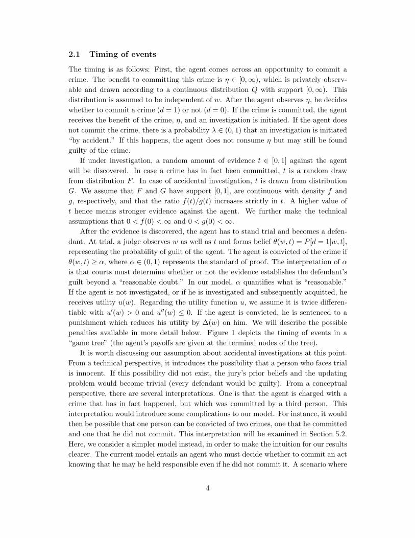
2.1 Timing of events

The timing is as follows: First, the agent comes across an opportunity to commit acrime. The benefit to committing this crime is η ∈ [0,∞), which is privately observ-able and drawn according to a continuous distribution Q with support [0,∞). Thisdistribution is assumed to be independent of w. After the agent observes η, he decideswhether to commit a crime (d = 1) or not (d = 0). If the crime is committed, the agentreceives the benefit of the crime, η, and an investigation is initiated. If the agent doesnot commit the crime, there is a probability λ ∈ (0, 1) that an investigation is initiated“by accident.” If this happens, the agent does not consume η but may still be foundguilty of the crime.

If under investigation, a random amount of evidence t ∈ [0, 1] against the agentwill be discovered. In case a crime has in fact been committed, t is a random drawfrom distribution F . In case of accidental investigation, t is drawn from distributionG. We assume that F and G have support [0, 1], are continuous with density f andg, respectively, and that the ratio f(t)/g(t) increases strictly in t. A higher value oft hence means stronger evidence against the agent. We further make the technicalassumptions that 0 < f(0) < ∞ and 0 < g(0) < ∞.

After the evidence is discovered, the agent has to stand trial and becomes a defen-dant. At trial, a judge observes w as well as t and forms belief θ(w, t) = P [d = 1|w, t],representing the probability of guilt of the agent. The agent is convicted of the crime ifθ(w, t) ≥ α, where α ∈ (0, 1) represents the standard of proof. The interpretation of α

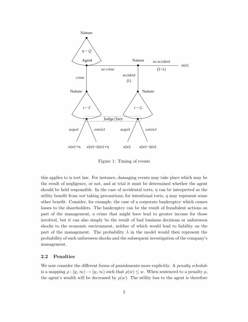
is that courts must determine whether or not the evidence establishes the defendant’sguilt beyond a “reasonable doubt.” In our model, α quantifies what is “reasonable.”If the agent is not investigated, or if he is investigated and subsequently acquitted, hereceives utility u(w). Regarding the utility function u, we assume it is twice differen-tiable with u′(w) > 0 and u′′(w) ≤ 0. If the agent is convicted, he is sentenced to apunishment which reduces his utility by ∆(w) on him. We will describe the possiblepenalties available in more detail below. Figure 1 depicts the timing of events in a“game tree” (the agent’s payoffs are given at the terminal nodes of the tree).

It is worth discussing our assumption about accidental investigations at this point.From a technical perspective, it introduces the possibility that a person who faces trialis innocent. If this possibility did not exist, the jury’s prior beliefs and the updatingproblem would become trivial (every defendant would be guilty). From a conceptualperspective, there are several interpretations. One is that the agent is charged with acrime that has in fact happened, but which was committed by a third person. Thisinterpretation would introduce some complications to our model. For instance, it wouldthen be possible that one person can be convicted of two crimes, one that he committedand one that he did not commit. This interpretation will be examined in Section 5.2.Here, we consider a simpler model instead, in order to make the intuition for our resultsclearer. The current model entails an agent who must decide whether to commit an actknowing that he may be held responsible even if he did not commit it. A scenario where

4

Nature

Nature

NatureNature

η ~ Q

(λ)accident

(1−λ)

no accidentAgent

no crime

crime

t ~ Gt ~ F

Judge/Jury

acquit convictacquit convict

u(w) u(w)−Δ(w)u(w)−Δ(w) +ηu(w) +η

u(w)

Figure 1: Timing of events

this applies to is tort law. For instance, damaging events may take place which may bethe result of negligence, or not, and at trial it must be determined whether the agentshould be held responsible. In the case of accidental torts, η can be interpreted as theutility benefit from not taking precautions; for intentional torts, η may represent someother benefit. Consider, for example, the case of a corporate bankruptcy which causeslosses to the shareholders. The bankruptcy can be the result of fraudulent actions onpart of the management, a crime that might have lead to greater income for thoseinvolved, but it can also simply be the result of bad business decisions or unforeseenshocks to the economic environment, neither of which would lead to liability on thepart of the management. The probability λ in the model would then represent theprobability of such unforeseen shocks and the subsequent investigation of the company’smanagement.

2.2 Penalties

We now consider the different forms of punishments more explicitly. A penalty scheduleis a mapping ρ : [w,∞) → [w,∞) such that ρ(w) ≤ w. When sentenced to a penalty ρ,the agent’s wealth will be decreased by ρ(w). The utility loss to the agent is therefore

5

∆(w) = u(w)− u(w − ρ(δ)). Listed below are a few important cases of penalties.

Imprisonment. If sentenced to prison, the agent’s wealth will be reduced to a uni-formly low level w0, which is independent of the agent’s type outside of prison. Thus,a prison sentence is given by the penalty schedule ρ(w) = w − w0. The utility loss tothe agent is therefore ∆(w) = u(w)− u(w0).

Simple fine. If sentenced to pay a simple fine, the agent’s wealth will be decreased bya fixed amount δ. This is described by the penalty schedule ρ(w) = δ, and the utilityloss to the agent is ∆(w) = u(w)− u(w − δ).

Proportional fine. If sentenced to pay a proportional fine, the agent’s wealth isreduced by a fraction γ ∈ (0, 1); thus ρ(w) = γw. The utility loss to the agent istherefore ∆(w) = u(w)− u((1− γ)w).

Since the utility loss ∆ depends on the type of punishment being used, differentpenalty forms have different effects on individuals of lower and higher income types.In general, it depends on both the properties of the utility function u as well as onproperties of the penalty schedule ρ whether higher or lower types are penalized moreseverely. However, if punishment is imprisonment, ∆ increases in w, so a prison sentenceclearly is a more severe punishment for higher types than it is for lower types. If thepunishment is a fine δ, on the other hand, ∆ decreases in w as long as agents arestrictly risk averse. In this case, a simple fine works exactly in the opposite directionas a prison sentence.

2.3 Bayesian beliefs at trial

At trial, the judge forms the posterior belief θ(w, t) through Bayesian updating. Specif-ically, let p(w) denote the judge’s prior belief that an individual of type w commitsa crime6. We will call p(w) the prejudice held against individuals of type w. TheBayesian likelihood that the investigated individual of type w is guilty, conditioning onevidence t, is then

θ(w, t) ≡ P [d = 1|w, t] =p(w)f(t)

p(w)f(t) + λ(1− p(w))g(t)∈ [0, 1]. (1)

Given that f(t)/g(t) increases, θ(w, t) increases in t and in p(w). For a fixed α, let t(w)be such that

α = θ(w, t(w));

t(w) is then the conviction threshold that is applied to individuals of type w. While α

is fixed for all defendants, the amount of evidence t(w) required to prove guilt beyondprobability α can depend on income w.

6Note that this prior is not subjective. In equilibrium, it is equal to the probability that an individual

of type w actually commits a crime. As such, judges will not differ in their priors.

6

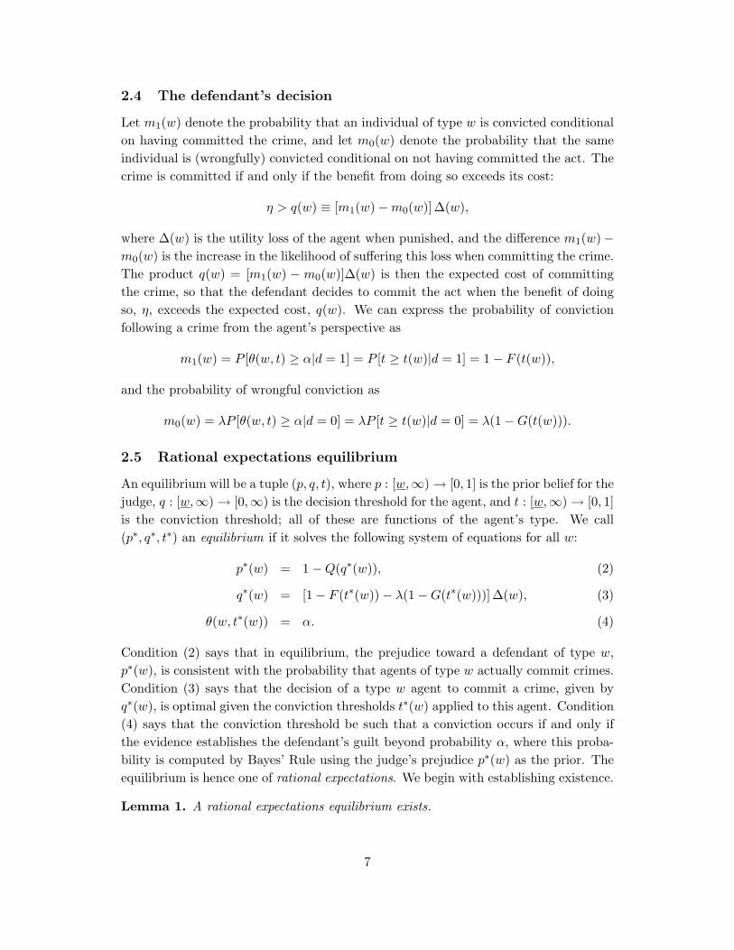
2.4 The defendant’s decision

Let m1(w) denote the probability that an individual of type w is convicted conditionalon having committed the crime, and let m0(w) denote the probability that the sameindividual is (wrongfully) convicted conditional on not having committed the act. Thecrime is committed if and only if the benefit from doing so exceeds its cost:

η > q(w) ≡ [m1(w)−m0(w)]∆(w),

where ∆(w) is the utility loss of the agent when punished, and the difference m1(w)−m0(w) is the increase in the likelihood of suffering this loss when committing the crime.The product q(w) = [m1(w) − m0(w)]∆(w) is then the expected cost of committingthe crime, so that the defendant decides to commit the act when the benefit of doingso, η, exceeds the expected cost, q(w). We can express the probability of convictionfollowing a crime from the agent’s perspective as

m1(w) = P [θ(w, t) ≥ α|d = 1] = P [t ≥ t(w)|d = 1] = 1− F (t(w)),

and the probability of wrongful conviction as

m0(w) = λP [θ(w, t) ≥ α|d = 0] = λP [t ≥ t(w)|d = 0] = λ(1−G(t(w))).

2.5 Rational expectations equilibrium

An equilibrium will be a tuple (p, q, t), where p : [w,∞) → [0, 1] is the prior belief for thejudge, q : [w,∞) → [0,∞) is the decision threshold for the agent, and t : [w,∞) → [0, 1]is the conviction threshold; all of these are functions of the agent’s type. We call(p∗, q∗, t∗) an equilibrium if it solves the following system of equations for all w:

p∗(w) = 1−Q(q∗(w)), (2)

q∗(w) = [1− F (t∗(w))− λ(1−G(t∗(w)))]∆(w), (3)

θ(w, t∗(w)) = α. (4)

Condition (2) says that in equilibrium, the prejudice toward a defendant of type w,p∗(w), is consistent with the probability that agents of type w actually commit crimes.Condition (3) says that the decision of a type w agent to commit a crime, given byq∗(w), is optimal given the conviction thresholds t∗(w) applied to this agent. Condition(4) says that the conviction threshold be such that a conviction occurs if and only ifthe evidence establishes the defendant’s guilt beyond probability α, where this proba-bility is computed by Bayes’ Rule using the judge’s prejudice p∗(w) as the prior. Theequilibrium is hence one of rational expectations. We begin with establishing existence.

Lemma 1. A rational expectations equilibrium exists.

7

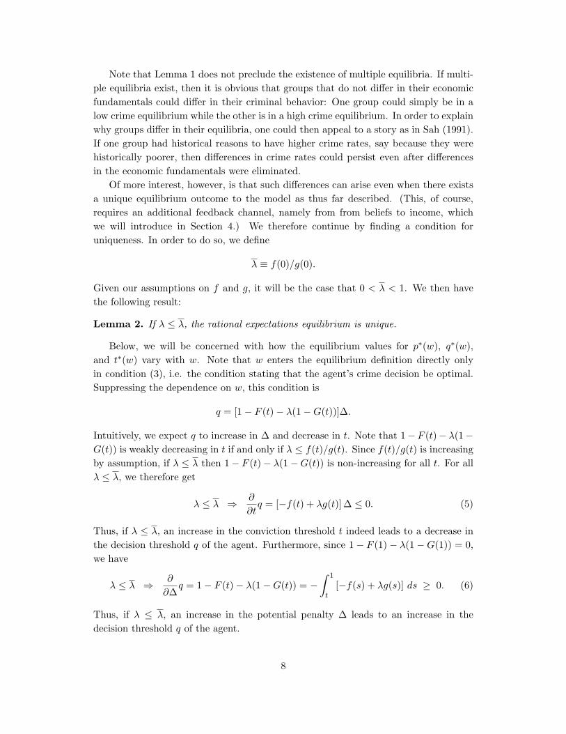
Note that Lemma 1 does not preclude the existence of multiple equilibria. If multi-ple equilibria exist, then it is obvious that groups that do not differ in their economicfundamentals could differ in their criminal behavior: One group could simply be in alow crime equilibrium while the other is in a high crime equilibrium. In order to explainwhy groups differ in their equilibria, one could then appeal to a story as in Sah (1991).If one group had historical reasons to have higher crime rates, say because they werehistorically poorer, then differences in crime rates could persist even after differencesin the economic fundamentals were eliminated.

Of more interest, however, is that such differences can arise even when there existsa unique equilibrium outcome to the model as thus far described. (This, of course,requires an additional feedback channel, namely from from beliefs to income, whichwe will introduce in Section 4.) We therefore continue by finding a condition foruniqueness. In order to do so, we define

λ ≡ f(0)/g(0).

Given our assumptions on f and g, it will be the case that 0 < λ < 1. We then havethe following result:

Lemma 2. If λ ≤ λ, the rational expectations equilibrium is unique.

Below, we will be concerned with how the equilibrium values for p∗(w), q∗(w),and t∗(w) vary with w. Note that w enters the equilibrium definition directly onlyin condition (3), i.e. the condition stating that the agent’s crime decision be optimal.Suppressing the dependence on w, this condition is

q = [1− F (t)− λ(1−G(t))]∆.

Intuitively, we expect q to increase in ∆ and decrease in t. Note that 1− F (t)− λ(1−G(t)) is weakly decreasing in t if and only if λ ≤ f(t)/g(t). Since f(t)/g(t) is increasingby assumption, if λ ≤ λ then 1− F (t)− λ(1−G(t)) is non-increasing for all t. For allλ ≤ λ, we therefore get

λ ≤ λ ⇒ ∂

∂tq = [−f(t) + λg(t)]∆ ≤ 0. (5)

Thus, if λ ≤ λ, an increase in the conviction threshold t indeed leads to a decrease inthe decision threshold q of the agent. Furthermore, since 1− F (1)− λ(1−G(1)) = 0,we have

λ ≤ λ ⇒ ∂

∂∆q = 1− F (t)− λ(1−G(t)) = −

∫ 1

t[−f(s) + λg(s)] ds ≥ 0. (6)

Thus, if λ ≤ λ, an increase in the potential penalty ∆ leads to an increase in thedecision threshold q of the agent.

8

These preliminary observations allow us to characterize the equilibrium further. Inparticular, we will state several results concerning prejudice. We call an equilibriumbiased against lower types if

w > w′ ⇒ p∗(w) < p∗(w′), t∗(w) > t∗(w′), and q∗(w) > q∗(w′).

That is, the judge is prejudiced in favor of higher types and applies a higher convictionthreshold to higher types, and higher types are less likely to commit a crime. Similarly,an equilibrium biased against higher types if the reverse inequalities hold:

w > w′ ⇒ p∗(w) > p∗(w′), t∗(w) < t∗(w′), and q∗(w) < q∗(w′).

Finally, if p∗, q∗ and t∗ are constant, the equilibrium is unbiased. hold:

w > w′ ⇒ p∗(w) > p∗(w′), t∗(w) < t∗(w′), and q∗(w) < q∗(w′).

Finally, if p∗, q∗ and t∗ are constant, the equilibrium is unbiased.

3 Penalties and Equilibrium Bias

We begin with a general result concerning the potential bias that can arise in equilib-rium. (As before, we assume that the defendant’s income w is exogenously given andobserved by the jury.)

Lemma 3. Suppose 0 < λ ≤ λ, and let (p∗, q∗, t∗) be the unique equilibrium. Theequilibrium is (i) biased against higher types when ∆ strictly decreases in w, (ii) biasedagainst lower types when ∆ strictly increases in w, and is (iii) unbiased if ∆ is constant.

With this result in mind, we are now ready to compare different forms of punishmentwith respect to whether they lead to biased equilibria or not, and if they do, whetherthe bias is against lower types or against higher types. In our analysis, punishmentsdiffer only in terms the utility loss ∆(w), they impose on defendants of type w. Thefollowing results are therefore all direct consequences of Lemma 3.

We begin by describing the general penalty schedule that leads to unbiased equi-libria. By Lemma 3, the equilibrium is unbiased if ∆ is a constant, i.e. ∆(w) = ∆ or∆′(w) = 0 ∀w:

∆′(w) = u′(w)− (1− ρ′(w))u′(w − ρ(w)) = 0, (7)

so that unbiasedness requires ρ to satisfy the following differential equation and initialcondition:

ρ′(w) = 1− u′(w)u′(w − ρ(w))

, (8)

ρ(w) = w − u−1(u(w)−∆), (9)

9

Condition (9) describes the punishment applicable to type w to achieve the desiredutility loss ∆. The differential equation (9) then describes how to trace out the penaltyschedule ρ that maintains the same utility loss for all types.7 This particular penaltyschedule, given in (9), describes a knife-edge case in that it characterizes those penaltieswhich lead to unbiased equilibria. Before turning to biased equilibria, we show thatthe knife-edge case can be achieved by simple and proportional fines, respectively, ifthe utility function u satisfies particular properties:

Theorem 4. The equilibrium is unbiased in the following special cases:

(a) Punishment is by a simple fine and agents are risk-neutral, i.e. u′′(w) < 0 ∀w.

(b) Punishment is by a proportional fine and agents have constant relative risk aver-sion of 1. That is, ρ(w) = γw for some γ ∈ (0, 1), and u(w) = a lnw + b forsome b and some a > 0.

Let us now consider under which conditions the equilibrium is biased. By Lemma3, ∆′(w) > 0 implies that the equilibrium will be biased against lower types. We cantherefore derive a condition similar to (9), that is, the equilibrium is biased againstlower types if the penalty schedule satisfies

ρ′(w) > 1− u′(w)u′(w − ρ(w))

.

Likewise, it is biased against higher types if the reverse inequality holds,

ρ′(w) < 1− u′(w)u′(w − ρ(w))

.

Of course, given any schedule ρ, it need not be the case that the equilibrium is monotonein w, as the resulting ∆(w) may not be monotone in w. As far as prison sentences andsimple fines are concerned, however, we can make the following statement:

Theorem 5. Suppose 0 < λ ≤ λ, and let (p∗, q∗, t∗) be the unique equilibrium.

(a) If punishment for convicted agents is by imprisonment, then (p∗, q∗, t∗) is biasedagainst lower types.

(b) If punishment for convicted agents is by a simple fine, and agents are strictly riskaverse (i.e. u′′(w) < 0 ∀w), then (p∗, q∗, t∗) is biased against higher types.

7Note that (9)–(9) describe the solution to a design problem which is not unlike the classical mech-

anism design problem. Similar to an incentive compatibility constraint, the unbiasedness requirement

leads to a solution in terms of the slope of the design object, and similar to an individual rationality

constraint, the fact that a certain deterrence effect must be created for the lowest type yields an initial

condition.

10

In general, the shape of ∆ depends on the shape of the both the utility functionu and the penalty schedule ρ. In the following, we derive sufficient conditions formonotonicity of ∆, and hence for a bias in favor of higher or lower types, respectively.Let R(w) denote the coefficient of relative risk aversion of u at w:

R(w) = −wu′′(w)u′(w)

.

Further, let ε(w) denote the income elasticity of ρ at w:

ε(w) = wρ′(w)ρ(w)

.

We can then show that the following holds:

Theorem 6. Suppose punishment for convicted agents is given by penalty schedule ρ.Suppose 0 < λ ≤ λ, and let (p∗, q∗, t∗) be the unique equilibrium. Then (p∗, q∗, t∗) isbiased against higher types if R(w) > 1 and ε(w) ≤ 1 ∀w, and it is biased against lowertypes if R(w) < 1 and ε(w) ≥ 1 ∀w.

Hence, it is possible to extend the result of Theorem 4 (b): In the special case of aproportional fine, the income elasticity of the fine is zero, i.e. ε(w) = 0. Whether theequilibrium is biased against lower or higher types depends then only on whether thecoefficient of relative risk aversion R(w) is always below or above one.

It should be noted that, even when the equilibrium is biased, the judges’s preju-dice is consistent with the true likelihood that agents of various types commit crimes.Furthermore, in equilibrium agents with differing types take into account that there isa different chance of conviction if they commit a crime than for agents of other types.For example in the case of imprisonment, the prejudice against an agent is decreasingwith his type, so agents with higher types know that they are more likely to avoidpunishment when committing a crime. However, in equilibrium higher types are stillless likely to commit crime than lower types (i.e. q∗(w) > q∗(w′) if w > w′).

We have thus established conditions for the treatment an individual receives fromthe courts to be dependent on their wealth. The story thus far suggests, however, thatpeople of the same wealth, but that differ in other characteristics, should be treatedthe same. In the next section, we allow for income to be determined endogenously, andfind that bias in the courts based on wealth can in fact lead to bias based on othercharacteristics.

4 Non-economic Types and Statistical Discrimination

In this section, we dispose of the assumption that agents differ in terms of their incomesw ex-ante. We instead assume that all agents are ex-ante alike with respect to economiccharacteristics such as their productivity, human capital, etc., which can influence a

11

person’s income. There are now L ≥ 2 subgroups of the population, and membershipin one group is merely a label l ∈ {1, . . . , L} without economic significance. This labelcould be race, gender, nationality, or ethnicity.8 An agent’s group label is publiclyobservable, and all differences in the realized value of an agent’s income are the directresult of the bias held against the agent’s group in the justice system. If such realinter-group differences arise endogenously ex-post, then such outcomes are “sunspotequilibria.”

To justify the assumption that an agent’s income is a function of prejudice, notethat it may simply be harder for a person who is assumed to be more prone to criminalbehavior to find a job, or to find a high-paying job, resulting in lower income. Thiscan be the case for a myriad of reasons. Criminal activity may adversely affect anindividual’s productivity, or criminal activity may directly be targeted at the employer(e.g. stealing from a job site). Further, if there are training costs for new employeesand employers expect that members of certain groups are more likely to be convictedof a crime and be sent to jail, then hiring a member of the disadvantaged group hasa larger expected cost because this individual’s duration in employment is on averageshorter. Alternatively, the qualifications required to be employed at a given wage canbe costly to obtain and training must be paid by the individual in form of tuition orforegone income while at school. An individual’s decision to acquire these qualificationswill depend on their expected return, which will be lower for those individuals who arelikely to be incarcerated in the future. We do not focus on any particular such story,and instead take a reduced form approach. Specifically, we assume that there is aweakly decreasing and continuous function v : [0, 1] → [w,w] (w < w < ∞) whichdescribes an agent’s income as a function of the prejudice held against the group towhich he belongs.

Since the only observable difference between agents is that they belong to differentsubgroups of the population, replace the prejudice p(w) against persons of income w

by a prejudice pl against persons who belong to group l. Similarly, replace q(w) by ql,and t(w) by tl. An equilibrium in this case is now a collection (w∗

l , p∗l , q

∗l , t

∗l )l∈{1,...,L}

such that for all l ∈ {1, . . . , L},

p∗l = 1−Q(q∗l ), (10)

q∗l = [1− F (t∗l )− λ(1−G(t∗l )]∆l, (11)

θ(pl, t∗l ) = α, (12)

w∗l = v(p∗l ), (13)

where ∆l = u(w∗l ) − u(w∗

l − ρ(w∗l )) is defined as before. This is essentially the same

8Of course, what we call “non-economic characteristics” can also be a-priori correlated with eco-

nomically meaningful variables. A woman’s productivity as a lumberjack is presumably on average

lower than a man’s, and a French person may on average be a better food critic than a British person.

We assume such cases away in our model.

12

set of defining equations as (2)–(4), except that a fourth condition has been added(condition (13)). This condition states that the equilibrium income level of group l,w∗

l , must be consistent with the prejudice level p∗l held against group l. We now say anequilibrium is biased if there exist l, l′ ∈ {1, . . . , L} such that p∗l > p∗l′ . An equilibriumis unbiased if p∗1 = . . . = p∗L.

Equilibria can be constructed from the points of intersection of two curves in p-wspace. The first curve is the locus of all (p, w) pairs such that p = p∗(w), where p∗(w) isthe equilibrium prejudice against an individual of income w, given by (2) of the simplemodel. The second one is the graph of the income function v(p). Let

S = {(p, w) ∈ [0, 1]× [w,w] : p = p∗(v(p))}

be the set of all intersecting points of the two curves. An equilibrium in the model withendogenous income can then be constructed by assigning to each group l ∈ {1, . . . , L}a point in S, corresponding to the prejudice p∗l against group l, and the income levelw∗

l of its members. The conviction threshold applied to defendants from group l, t∗lcan then be computed from (12), and the decision threshold which agents from groupl use, q∗l , can be computed from (11).

If S 6= ∅, then an equilibrium exists. The following states a sufficient condition forexistence:

Lemma 7. Regardless of the punishment used, if 0 < λ ≤ λ there exists an equilibriumin the model with endogenous income.

If an equilibrium exists, there is always an unbiased equilibrium, as all groupscan be assigned the same (p, w)-pair. Whenever S contains more than one element,there are also biased equilibria, as any assignment of groups to (p, w)-pairs containedin S represents an equilibrium in the extended model. Thus, if |S| > 1, there is anequilibrium in which p∗l 6= p∗l′ for l 6= l′, and also w∗

l 6= w∗l′ , namely if (p∗l , w

∗l ) ∈ S and

(p∗l′ , w∗l′) ∈ S. The following result mirrors Lemma 3.

Lemma 8. Fix w > 0 and w > w. Let D be the set of all continuous, decreasingfunctions v : [0, 1] → [w,w]. Suppose λ ≤ λ.

(a) If ∆ strictly decreases in w, or is constant, then for all v ∈ D there is a uniqueequilibrium, and this equilibrium is unbiased.

(b) If ∆ increases in w, there exists a non-empty set D0 ⊂ D such that for all v ∈ D0,a biased equilibrium exists.

The next result follows then immediately from Lemma 8 (a proof is therefore omit-ted):

Theorem 9. Fix w > 0 and w > w. Let D be the set of all continuous, decreasingfunctions v : [0, 1] → [w,w]. Suppose λ ≤ λ.

13

(a) If convicted offenders are punished by a simple fine, then for all v ∈ D there is aunique equilibrium, and this equilibrium is unbiased.

(b) If convicted offenders are punished by imprisonment, there exists a non-empty setD0 ⊂ D such that for all v ∈ D0 a biased equilibrium exists.

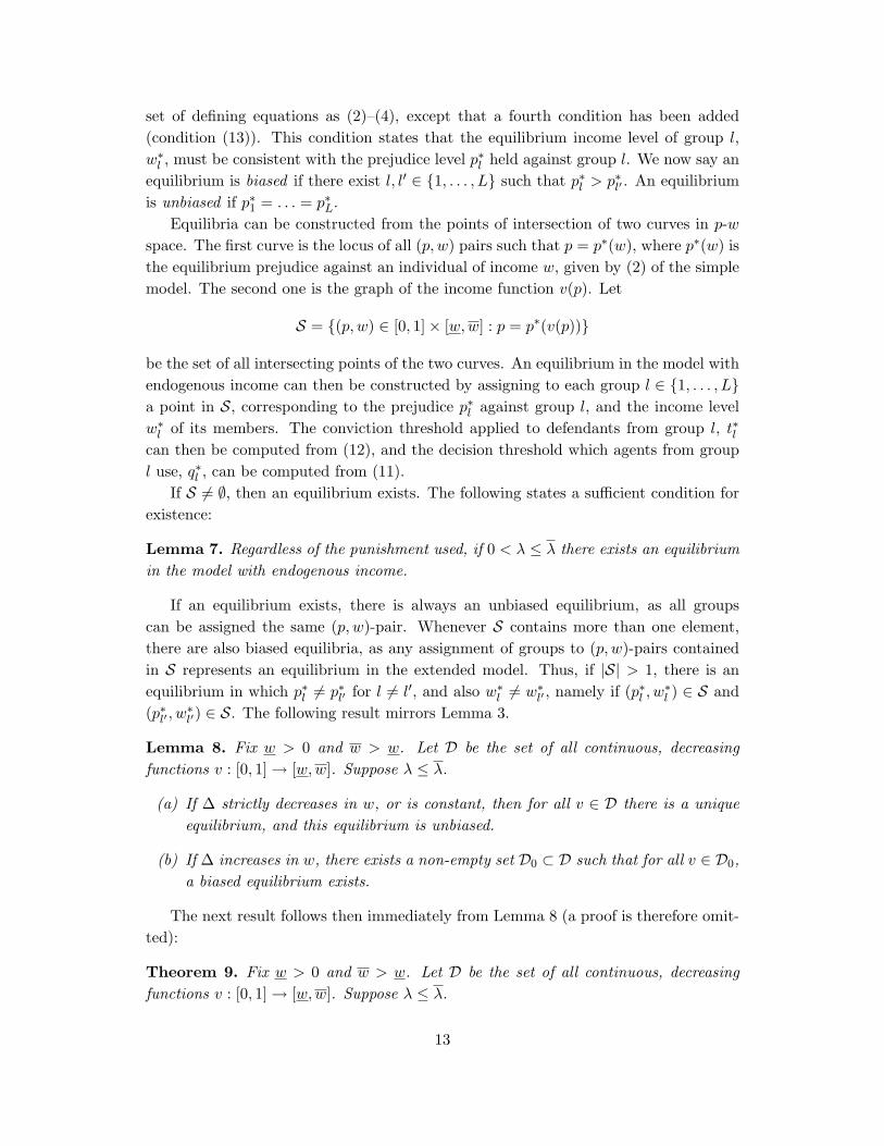
Figure 2 depicts the case of Theorem 9 (b), where v ∈ D0. It is worth mentioningthat there is nothing “special” about the function v depicted. That is, this resultdoes not rely on there being any points of tangency or discontinuities, and the set D0

could be loosely be regarded as “generic.”9 In general, there will be a relatively largenumber of functions v ∈ D0. With prison as punishment for convicted agents, thep∗-curve is increasing, and it is not hard to plot a continuous and decreasing v-curvewhich intersects the p∗-curve several times. In our example there are three intersections(|S| = 3), so that one can construct equilibria with up to three different endogenousincome levels. We depict an example with two groups: Group 1 earns a relatively highincome w∗

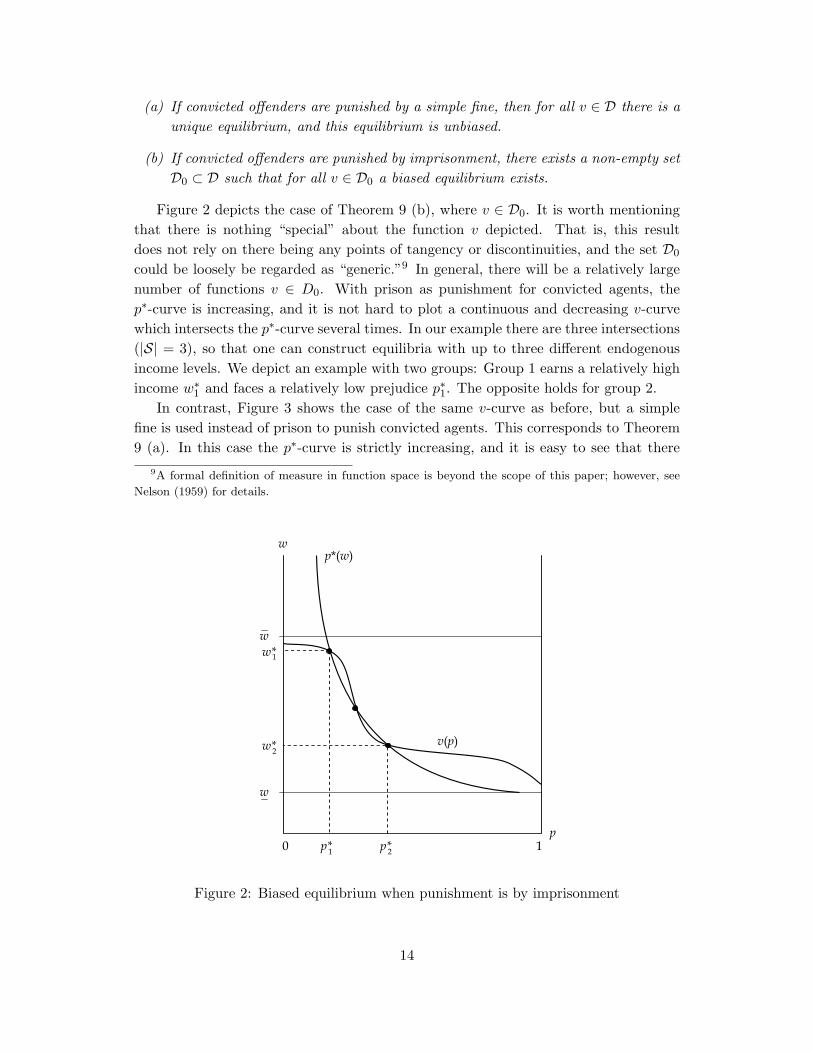
1 and faces a relatively low prejudice p∗1. The opposite holds for group 2.In contrast, Figure 3 shows the case of the same v-curve as before, but a simple

fine is used instead of prison to punish convicted agents. This corresponds to Theorem9 (a). In this case the p∗-curve is strictly increasing, and it is easy to see that there

9A formal definition of measure in function space is beyond the scope of this paper; however, see

Nelson (1959) for details.

0 1p

wp*(w)

v(p)w*

w*1

2

21 p*p*

w

w

Figure 2: Biased equilibrium when punishment is by imprisonment

14

cannot be multiple intersections of p∗ and v now. Thus the only equilibrium is anunbiased one, where both groups earn the same income and face the same prejudice.

21 =0 1

w

w

w

p*(w)

v(p)

w*2w*1 =

p*p*p

Figure 3: Unbiased equilibrium when simple fines are used

5 Extensions

In this section, we show how our model can be extended by introducing dynamics(Section 5.1) and the possibility of multiple offenses (Section 5.2). The merits of theseextensions are described in detail below.

5.1 A Dynamic Link from Prejudice to Income

When punishment is by imprisonment, we have shown that there exists a possibilityfor discriminatory equilibria, where racial groups differ in terms of their crime rates,but also in terms of their incomes. This required there to be some feedback from the(perceived) proclivity to crime of an individual to the individual’s income. We modeledthis feedback in “reduced form” by assuming there be a downward sloping function v

that mapped an individual’s perceived crime rate to income. In equilibrium of such amodel, both membership in a certain racial group, or an individual’s income, can thenexplain the likelihood that the individual is convicted of a crime. There is, however,empirical evidence (cited in the introduction) that race is a significant predictor ofcriminal activity after controlling for wages and a number of other economic variables.

15

In this section, we show that when introducing a temporal dimension to our model,this empirical observation can be reconciled. In particular, by using expected lifetimeearnings as the relevant income variable, we show that the sanctions imposed by thecourts on convicted criminals can be directly responsible for differences in lifetimeearnings.

Suppose employers offer (voluntarily or by law) the same wage to everybody, aslong as they possess the same economically relevant qualifications, such as academicdegrees or technical diplomas. However, members of one group are more likely to spendsome time of their lives in prison than others. They will hence receive the same wageas everybody else when they work, but over a stochastically shorter period of time. Forsimplicity, assume that only life sentences are given. Then individuals who face a strongprejudice on average will go to jail sooner—thus their expected lifetime earnings theystand to lose from the sentence are lower, compared to individuals who face a lesserprejudice. Consequently, they are less likely to be deterred by the threat of losing thisexpected future income, and more likely to commit crimes, making this an equilibriumagain. The difference is now that a worker’s per-period wage income has no predictivepower regarding criminal activity, but membership in racial groups has. Furthermore,it is not discrimination in the labor market, but the criminal justice system itself, thatprovides the causal link between prejudice and income. If wage differences exist thatare due to differential treatment by employers, affirmative action that mandates non-discriminatory treatment in the labor market could help eliminate this problem (similarto the argument made by Coate and Loury (1993)). However, in the case we considerhere, such policies will have no effect at best, as employers pay the same wage to allworkers already.

We assume that agents live for infinitely many periods. At the beginning of eachperiod, an agent will work and earn a fixed wage of y, unless he is in prison in whichcase he earns zero. There is no saving technology, and all income is consumed in theperiod it is earned. At the end of each period, the events described in Section 2 unfold:Agents observe their η-shocks and decide whether to commit the crime or not (theη-draws are assumed i.i.d. across agents and time), and must possibly stand trial. Atthe end of the period, the agent is then either a convicted criminal or not. If an agent isconvicted (rightfully or wrongfully), he is removed from employment and sentenced tolife in prison. This sentence represents a permanent reduction in income.10 Otherwise,the agent starts the next period as a working individual. In computing their expectedlifetime earnings, agents apply a common discount factor β < 1 and do not includethe future realizations of η. This is a behavioral assumption, of course, but unless η

is literally regarded as the material benefit from a crime (for instance money stolen),this assumption seems not unreasonable. For example, one interpretation of η is that

10We expect that the results we derive continue to hold for sufficiently long but finite prison sentences,

as the crucial feature of this penalty is not so much the duration of time over which it is applied, but

that it reduces the agent’s lifetime income to a fixed level.

16

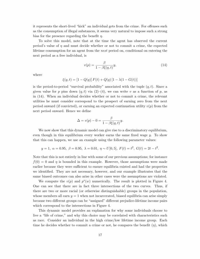
it represents the short-lived “kick” an individual gets from the crime. For offenses suchas the consumption of illegal substances, it seems very natural to impose such a strongbias for the presence regarding the benefit η.

To solve this model, note that at the time the agent has observed the currentperiod’s value of η and must decide whether or not to commit a crime, the expectedlifetime consumption for an agent from the next period on, conditional on entering thenext period as a free individual, is

v(p) =β

1− βξ(q, t)y, (14)

whereξ(q, t) = [1−Q(q)]F (t) + Q(q) [1− λ(1−G(t))]

is the period-to-period “survival probability” associated with the tuple (q, t). Since agiven value for p pins down (q, t) via (2)–(4), we can write v as a function of p, asin (14). When an individual decides whether or not to commit a crime, the relevantutilities he must consider correspond to the prospect of earning zero from the nextperiod onward (if convicted), or earning an expected continuation utility v(p) from thenext period onward. Hence we define

∆ = v(p)− 0 =β

1− βξ(q, t)y.

We now show that this dynamic model can give rise to a discriminatory equilibrium,even though in this equilibrium every worker earns the same fixed wage y. To showthat this can happen, we use an example using the following parameter values:

y = 1, α = 0.95, β = 0.95, λ = 0.01, η ∼ U [0, 5], F (t) = t2, G(t) = 2t− t2.

Note that this is not entirely in line with some of our previous assumptions; for instancef(0) = 0 and η is bounded in this example. However, those assumptions were madeearlier because they were sufficient to ensure equilibria existed and had the propertieswe identified. They are not necessary, however, and our example illustrates that thesame biased outcomes can also arise in other cases were the assumptions are violated.

We compute the v(p) and p∗(w) numerically. The result is plotted in Figure 4.One can see that there are in fact three intersections of the two curves. Thus, ifthere are two or more racial (or otherwise distinguishable) groups in the population,whose members all earn y = 1 when not incarcerated, biased equilibria can arise simplybecause two different groups can be “assigned” different prejudice-lifetime income pairswhich correspond to the intersections in Figure 4.

This dynamic model provides an explanation for why some individuals choose tolive a “life of crime,” and why this choice may be correlated with characteristics suchas race. Consider an individual in the high crime/low lifetime income group. Eachtime he decides whether to commit a crime or not, he compares the benefit (η), which

17

p

w

v(p)

p*(w)

Figure 4: Numerical example (v(p) is expected discounted lifetime income)

is distributed equally across the entire population, against the expected cost. Theexpected cost is that the individual (with some probability) loses his criminal careerand goes to jail. However, continuing a life of crime is not a very enticing prospecteither, because a career criminal expects to be jailed sooner or later anyways. Hence,such a person is less likely to be deterred by this prospect. The opposite holds for thechoice to live a low-crime life, and the usual stereotyping argument can be made tosort individuals into different such equilibria, based on their race or other observablecharacteristics. The crucial aspect here is that, because race is observable and cannotbe altered, it is not possible for individuals to break out of the high-crime equilibrium—they would be treated in an adverse manner by the courts even if they decided not tocommit crime ever. Note that this result relies on the difference in the deterrence effectthat long prison sentence have for members of the different subgroups. The same storycould not be told in an alternative framework where instead of the cost of crime thebenefit was different across groups (as would be the case, for example, if we focused onproperty crime and assumed that poorer individuals could gain more from stealing).

5.2 Multiple Offenses and Escalating Sanctions

In this section, we drop the interaction with the labor market. That is, we now considerindividuals without regard to their income or wealth. As in Section 4, we consider L ≥ 2subgroups of the population, where members of these subgroups do not differ in anymeaningful way. The timing is as before, with the exception that, when agents decide

18

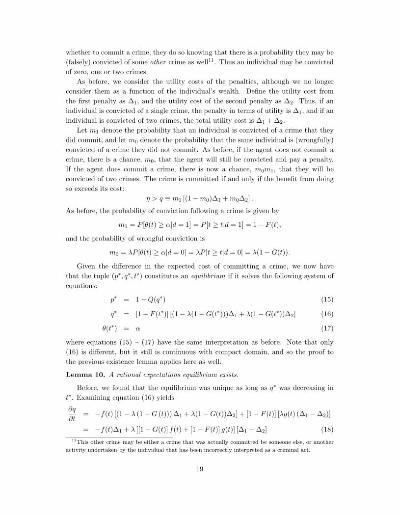
whether to commit a crime, they do so knowing that there is a probability they may be(falsely) convicted of some other crime as well11. Thus an individual may be convictedof zero, one or two crimes.

As before, we consider the utility costs of the penalties, although we no longerconsider them as a function of the individual’s wealth. Define the utility cost fromthe first penalty as ∆1, and the utility cost of the second penalty as ∆2. Thus, if anindividual is convicted of a single crime, the penalty in terms of utility is ∆1, and if anindividual is convicted of two crimes, the total utility cost is ∆1 + ∆2.

Let m1 denote the probability that an individual is convicted of a crime that theydid commit, and let m0 denote the probability that the same individual is (wrongfully)convicted of a crime they did not commit. As before, if the agent does not commit acrime, there is a chance, m0, that the agent will still be convicted and pay a penalty.If the agent does commit a crime, there is now a chance, m0m1, that they will beconvicted of two crimes. The crime is committed if and only if the benefit from doingso exceeds its cost:

η > q ≡ m1 [(1−m0)∆1 + m0∆2] .

As before, the probability of conviction following a crime is given by

m1 = P [θ(t) ≥ α|d = 1] = P [t ≥ t|d = 1] = 1− F (t),

and the probability of wrongful conviction is

m0 = λP [θ(t) ≥ α|d = 0] = λP [t ≥ t|d = 0] = λ(1−G(t)).

Given the difference in the expected cost of committing a crime, we now havethat the tuple (p∗, q∗, t∗) constitutes an equilibrium if it solves the following system ofequations:

p∗ = 1−Q(q∗) (15)

q∗ = [1− F (t∗)] [(1− λ(1−G(t∗)))∆1 + λ(1−G(t∗))∆2] (16)

θ(t∗) = α (17)

where equations (15) – (17) have the same interpretation as before. Note that only(16) is different, but it still is continuous with compact domain, and so the proof tothe previous existence lemma applies here as well.

Lemma 10. A rational expectations equilibrium exists.

Before, we found that the equilibrium was unique as long as q∗ was decreasing int∗. Examining equation (16) yields

∂q

∂t= −f(t) [(1− λ (1−G (t)))∆1 + λ(1−G(t))∆2] + [1− F (t)] [λg(t) (∆1 −∆2)]

= −f(t)∆1 + λ [[1−G(t)] f(t) + [1− F (t)] g(t)] [∆1 −∆2] (18)11This other crime may be either a crime that was actually committed be someone else, or another

activity undertaken by the individual that has been incorrectly interpreted as a criminal act.

19

and we have proved the following lemma:

Lemma 11. The rational expectations equilibrium is unique when ∆2 > ∆1.

When the equilibrium is not unique, stereotyping equilibria are possible, as wasdepicted previously in Figure 2. As long as second penalties are more severe in theirutility costs, crime rates are uniquely determined across subgroups and there will be nostereotyping equilibrium. It should be noted that, with respect to fines, the utility costof punishment is increasing (∆2 > ∆1) even when the amount of the fine is independentof the number of convictions because of diminishing marginal utility. However, withprison, the second conviction is likely to be less severe. Possible reasons for this includediscounting (a second penalty occurs after the first has been served) and a general loss ofsocial status, and perhaps employment and marital status as well, that occurs after thefirst conviction. As a result, if incarceration is used as punishment, prison terms thatincrease in the number of convictions would be desirable. Note that this provides anadditional rationale for increasing (or at least non-decreasing) penalties, to complementthe work of Emons (2006) and Stigler (1970). Note that even when the equilibrium isunique, it is still possible for groups that vary in non-economic characteristics (such asrace) to differ in their crime rates through the mechanism described in section 4.

6 Conclusion

We developed a model that tied jury prejudice, the decision to commit crime, andconviction standards into a single framework. Within this framework, we were able tocharacterize the effects of different penalty forms, such as prison sentences or mone-tary sanctions, on beliefs and thus also on behavior. Making prejudice (i.e. beliefs)endogenous in the model allowed us to develop from it a theory of discrimination basedon non-economic characteristics such as race. We now conclude the paper with a cou-ple of remarks, concerning the implications of the paper and possible areas of furtherresearch.

First, our results have implications for the design, or reform, of criminal justicesystems. We have compared the different effects of prison and monetary sentences onprejudice; the former being more likely to invite stereotyping than the latter. We donot intend to give a thorough survey of the advantages and disadvantages of fines vs.prison sentences here. Nevertheless, we think our model has something to say aboutthe various forms of penalizing felonies such as minor drug offenses. In the U.S. suchcrimes are routinely punished by incarceration, while European countries tend to usefines. The example of drug offenses is particularly interesting, as drug-related crimeis responsible for a large fraction of the U.S. prison population12. In addition, those

12About 55% of Federal inmates in 2003 and 25% of state level inmates were incarcerated for drug-

related offenses. Source: Bureau of Justice Statistics Prisoners in 2004, NCJ 210677, October 2005.

20

convicted for drug-related offenses are disproportionately Black or Hispanic13. If thepossibility of statistical discrimination is a concern to those who draft sentencing laws,then the relationship between different forms of penalties and the effects they have oncrime and prejudice should be taken seriously.

Second, note that our model (with prison sentences) produced two related phenom-ena: In the static version, sunspot equilibria could emerge in which people were treateddifferently by the courts based on their race. In such equilibria, the group which faceda less favorable judicial prejudice was also ex-post economically disadvantaged. In thedynamic version of Section 5.1, we constructed an example that possessed a similarsunspot equilibrium; however, the group with the less favorable prejudice was disad-vantaged only in terms of their lifetime earnings, and not in terms of their per-periodearnings when at work. Obviously, a more elaborate model can be conceived in whichboth aspects arise: The disadvantaged racial group has on average lower wages thanthe advantaged one, for the reasons mentioned in the text, but race has residual pre-dictive power of criminal activity. This pattern exists very clearly in the data (see thereferences cited in the introduction), and we regard the lifetime income model as apromising theoretical framework in which to explore this issue further.

Finally, we have shown that the model can be extended to multiple offenses andmore complex penalty schedules which are functions of the number of previous convic-tions. Examining the effects of escalating sanctions in the dynamic model is likely toproduce interesting results. One rationale for escalating sanctions is that convicted of-fenders can be of two types: Those who are corrigible (and deserve a “second chance”)and those who are not (and from which the public should be protected). A personconvicted of multiple offenses is more likely to belong to the second category; hence theincreasing sentences for repeat offenders.14 It appears that in a dynamic model, wherecrime decisions are based on lifetime expected income, the number of prior convictionscould serve a similar role as race in our model: If persons with prior convictions facean unfavorable prejudice in the legal system, then they may be more likely to commitcrimes, which may make them appear to be incorrigible. Exploring this possibility isanother question left for future research.

13Blacks and Hispanics represented 24% and 23% of those convicted for drug-related offenses in 2003,

compared to 14% Whites. Source: Prisoners in 2005, NCJ 215092, November 2006.14An alternative justification for escalating sanctions is given in Emons (2006).

21

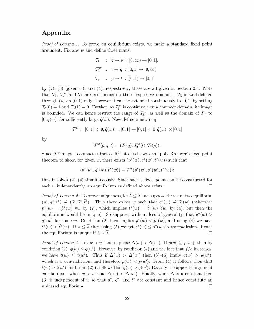
Appendix

Proof of Lemma 1. To prove an equilibrium exists, we make a standard fixed pointargument. Fix any w and define three maps,

T1 : q → p : [0,∞) → [0, 1],

T w2 : t → q : [0, 1] → [0,∞),

T3 : p → t : (0, 1) → [0, 1]

by (2), (3) (given w), and (4), respectively; these are all given in Section 2.5. Notethat T1, T w

2 and T3 are continuous on their respective domains. T3 is well-definedthrough (4) on (0, 1) only; however it can be extended continuously to [0, 1] by settingT3(0) = 1 and T3(1) = 0. Further, as T w

2 is continuous on a compact domain, its imageis bounded. We can hence restrict the range of T w

2 , as well as the domain of T1, to[0, q̂(w)] for sufficiently large q̂(w). Now define a new map

T w : [0, 1]× [0, q̂(w)]× [0, 1] → [0, 1]× [0, q̂(w)]× [0, 1]

byT w(p, q, t) = (T1(q), T w

2 (t), T3(p)).

Since T w maps a compact subset of R3 into itself, we can apply Brouwer’s fixed pointtheorem to show, for given w, there exists (p∗(w), q∗(w), t∗(w)) such that

(p∗(w), q∗(w), t∗(w)) = T w(p∗(w), q∗(w), t∗(w));

thus it solves (2)–(4) simultaneously. Since such a fixed point can be constructed foreach w independently, an equilibrium as defined above exists.

Proof of Lemma 2. To prove uniqueness, let λ ≤ λ and suppose there are two equilibria,(p∗, q∗, t∗) 6= (p̃∗, q̃∗, t̃∗). Thus there exists w such that q∗(w) 6= q̃∗(w) (otherwisep∗(w) = p̃∗(w) ∀w by (2), which implies t∗(w) = t̃∗(w) ∀w, by (4), but then theequilibrium would be unique). So suppose, without loss of generality, that q∗(w) >

q̃∗(w) for some w. Condition (2) then implies p∗(w) < p̃∗(w), and using (4) we havet∗(w) > t̃∗(w). If λ ≤ λ then using (5) we get q∗(w) ≤ q̃∗(w), a contradiction. Hencethe equilibrium is unique if λ ≤ λ.

Proof of Lemma 3. Let w > w′ and suppose ∆(w) > ∆(w′). If p(w) ≥ p(w′), then bycondition (2), q(w) ≤ q(w′). However, by condition (4) and the fact that f/g increases,we have t(w) ≤ t(w′). Thus if ∆(w) > ∆(w′) then (5)–(6) imply q(w) > q(w′),which is a contradiction, and therefore p(w) < p(w′). From (4) it follows then thatt(w) > t(w′), and from (2) it follows that q(w) > q(w′). Exactly the opposite argumentcan be made when w > w′ and ∆(w) < ∆(w′). Finally, when ∆ is a constant then(3) is independent of w so that p∗, q∗, and t∗ are constant and hence constitute anunbiased equilibrium.

22

Proof of Theorem 4. If u′′(w) = 0, then ∆′(w) = u′(w)− u′(w − δ) = 0, and Lemma 3(iii) implies (a). If ρ(w) = γw and u(w) = a lnw + b, then ∆′(w) = a/w − a/w = 0,and Lemma 3 (iii) implies (b) as well.

Proof of Theorem 5. In case of imprisonment, ∆(w) = u(w) − u0, which is strictlyincreasing in w since u′(w) > 0. Applying Lemma 3 (ii) yields (a). In case of a fine,∆(w) = u(w)− u(w − δ), which is strictly decreasing in w if u′′(w) < 0 ∀w. ApplyingLemma 3 (i) yields (b).

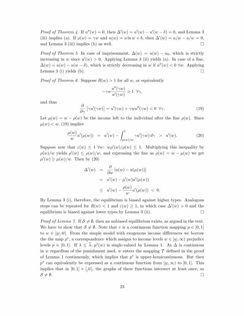
Proof of Theorem 6. Suppose R(w) > 1 for all w, or equivalently

−γwu′′(γw)u′(γw)

> 1 ∀γ,

and thus∂

∂γ

[γu′(γw)

]= u′(γw) + γwu′′(γw) < 0 ∀γ. (19)

Let µ(w) = w − ρ(w) be the income left to the individual after the fine ρ(w). Sinceµ(w) < w, (19) implies

µ(w)w

u′(µ(w)) = u′(w)−∫ 1

µ(w)/wγu′(γw) dγ > u′(w). (20)

Suppose now that ε(w) ≤ 1 ∀w: wρ′(w)/ρ(w) ≤ 1. Multiplying this inequality byρ(w)/w yields ρ′(w) ≤ ρ(w)/w, and expressing the fine as ρ(w) = w − µ(w) we getµ′(w) ≥ µ(w)/w. Then by (20)

∆′(w) =∂

∂w[u(w)− u(µ(w))]

= u′(w)− µ′(w)u′(µ(w))

≤ u′(w)− ρ(w)w

u′(µ(w)) < 0.

By Lemma 3 (i), therefore, the equilibrium is biased against higher types. Analogoussteps can be repeated for R(w) < 1 and ε(w) ≥ 1, in which case ∆′(w) > 0 and theequilibrium is biased against lower types by Lemma 3 (ii).

Proof of Lemma 7. If S 6= ∅, then an unbiased equilibrium exists, as argued in the text.We have to show that S 6= ∅. Note that v is a continuous function mapping p ∈ [0, 1]to w ∈ [w,w]. From the simple model with exogenous income differences we borrowthe the map p∗, a correspondence which assigns to income levels w ∈ [w,∞) prejudicelevels p ∈ [0, 1]. If λ ≤ λ, p∗(w) is single-valued by Lemma 1. As ∆ is continuousin w regardless of the punishment used, w enters the mapping T defined in the proofof Lemma 1 continuously, which implies that p∗ is upper-hemicontinuous. But thenp∗ can equivalently be expressed as a continuous function from [w,∞) to [0, 1]. Thisimplies that in [0, 1] × [,w], the graphs of these functions intersect at least once, soS 6= ∅.

23

Proof of Lemma 8. In the proof of Theorem 7 we already established that p∗ is a con-tinuous function from [w,∞) → [0, 1]. We first prove (a). Lemma 3 (i), p∗ strictlyincreases for strictly decreasing ∆. Therefore, for each v ∈ D there is exactly onew ∈ [0, 1] such that v(p∗(w)) = w. If ∆ is constant, then by Lemma 3 (iii) p∗ isconstant. It will hence become a vertical line in p-w space, which is intersected byany decreasing, continuous v exactly once. Hence |S| = 1 and a unique, unbiasedequilibrium exists. To prove (b), note that by Lemma 3 (ii) p∗ strictly decreases forstrictly increasing ∆. Therefore, there exists a non-empty set of continuous, decreasingfunctions v : [0, 1] → [w,w] for which the following holds: There exists w1, w2 ∈ [w,w],w1 6= w2, such that v(p∗(w1)) = w1 and v(p∗(w2)) = w2. For all such v, |S| > 1 and abiased equilibrium exists.

References

Alexeev, M. and J. Leitzel (2004): “Racial Profiling,”mimeo, Indiana University.

Arrow, K. (1973): “The Theory of Discrimination,” in: O. Ashenfelter and A. Rees(eds.): Discrimination in Labor Markets, Princeton University Press, 3–33.

Aumann, R. (1987): “Correlated Equilibrium as an Expression of Bayesian Rational-ity,” Econometrica, 55, 1–18.

Becker, G. (1957): The Economics of Discrimination, University of Chicago Press.

Becker, G. (1968): “Crime and Punishment: An Economic Approach,” Journal ofPolitical Economy, 76, 169–217.

Bjerk, D. (2006): “The Effects of Segregation on Crime Rates,” mimeo, McMasterUniversity.

Bjerk, D. (2007): “Racial Profiling, Statistical Discrimination, and the Effect of aColorblind Policy on the Crime Rate,” Journal of Public Economic Theory, forthcom-ing.

Burke, A. (2007): “Neutralizing Cognitive Bias: An Invitation to Prosecutors,”mimeo, Hofstra University School of Law.

Cartwright, E. and M. Wooders (2006): “Conformity, Correlation, and Equity,”mimeo, Vanderbilt University.

Cass, D. and K. Shell (1983): “Do Sunspots Matter?” Journal of Political Economy,91, 193–227.

24

Coate, S. and G. Loury (1993): “Will Affirmative-Action Policies Eliminate Nega-tive Stereotypes,” American Economic Review, 83, 1220–1240.

Emons, W. (2006): “Escalating Penalties for Repeat Offenders,” International Reviewof Law and Economics, forthcoming.

Forges, F. (1986): “An Approach to Communication Equilibria,” Econometrica, 54,1375–1385.

Georgakopoulos, N. (2004): “Self-fulfilling Impressions of Criminality: Uninten-tional Race Profiling,” International Review of Law and Economics, 24, 169–190.

Knowles, J., N. Persico, and P. Todd (2001): “Racial Bias in Motor-VehicleSearches: Theory and Evidence,” Journal of Political Economy, 109, 203–229.

Krivo, L. and R. Peterson (1996): “Extremely Disadvantaged Neighborhoods andUrban Crime,” Social Forces, 75, 619–650.

Levitt, S. (1997): “Incentive Compatibility Constraints as an Explanation for the Useof Prison Sentences Instead of Fines,” International Review of Law and Economics, 17,179–192.

Morris, N. and M. Tonry (1990): Between Prison and Probation, Oxford UniversityPress, Oxford.

Nelson, E. (1959): “Regular Probability Measure on Function Space,” Annals ofMathematics, 69, 630–643.

Persico, N. (2002): “Racial Profiling, Fairness, and Effectiveness of Policing,” Amer-ican Economic Review, 92, 1472–1497.

Phelps, E. (1972): “The Statistical Theory of Racism and Sexism,” American Eco-nomic Review, 62, 659–661.

Polinsky A. and S. Shavell (1984): “The Optimal Use of Fines and Imprisonment,”Journal of Public Economics, 24, 89–99.

Posner, R. (1992): Economic Analysis of Law, 4th Edition, Little, Brown and Com-pany, Boston.

Raphael, S. and R. Winter-Ebmer (2001): “Identifying the Effect of Unemploy-ment on Crime,” Journal of Law and Economics, 44, 259–283.

Sah, R. (1991): “Social Osmosis and Patterns of Crime,” Journal of Political Economy,99, 1272–1295.

25

Stigler, G. (1970): “The Optimum Enforcement of Laws,” Journal of Political Econ-omy, 78, 526–536.

Trumbull, W. (1989): “Estimations of the Economic Model of Crime Using Aggre-gate and Individual Level Data,” Southern Economic Journal, 56, 423–439.

Verdier, T. and Y. Zenou (2004): “Racial Beliefs, Location, and the Cause ofCrime,” International Economic Review, 45, 731–760.

26