data mining with mlps (and other methods) · great emphasis in using expert systems ... paulo...

Data Mining with Multilayer Perceptrons (and other methods)

Paulo [email protected]://www3.dsi.uminho.pt/pcortez

Department of Information Systems/Centro AlgoritmiUniversity of Minho - Campus de Azurem4800-058 Guimaraes - Portugal

Paulo Cortez Data Mining with MLPs (and other methods)

http://www3.dsi.uminho.pt/pcortez

About me: http://www3.dsi.uminho.pt/pcortez


http://www3.dsi.uminho.pt/pcortez

Motivation

World storage capacity in hard disk drives (in petabytes, source:http://www2.sims.berkeley.edu/research/projects/how-much-info-2003)

1995 1996 1997 1998 1999 2000 2001 2002 2003

050

0010

000

1500

0


http://www2.sims.berkeley.edu/research/projects/how-much-info-2003

Data Mining (DM)

Also known as Knowledge Discovery in Databases (KDD);

Definition [Fayyad et al., 1996]: “the overall process of discoveringuseful knowledge from data”;

In the Artificial Intelligence (AI) domain, in the 70s, there was agreat emphasis in using expert systems (mimic the expert);

The trend shifted in the 90s to intelligent systems and DM: learnfrom the data (i.e. data-driven models) or use hybrid approaches.


Business Intelligence (BI) and DM[Turban et al., 2010]

BI: “Umbrella term that includes architectures, tools, databases,applications and methodologies”. The goal of BI is to transform datainto information, then to decisions and finally actions;BI systems often use DM (for knowledge extraction andprediction).


DM Methodologies: CRISP-DM[Chapman et al., 2000]

Tool-neural process, developed to increase the success of DM projects(backed by SPSS and NCR). Consists of 6 iterative and interactive phases:

2. Data

−−??−−??? ....

....

....

1. BusinessUnderstanding

DataWarehouse/

Database

4. ModelingPreparation3. Data 5. Evaluation 6. Deployment

Predictive/Explanatory

Knowledge

Dataset Modelsprocessed

Pre−

Dataset

Understanding

Business Understanding: setting business goals, elaborating DMproject, selecting DM tool and personnel, ...;Data Understanding: merging data from multiple sources, checkingfor data integrity, data visualization, data statistics, ...;Data Preparation: handling missing data, outliers, selecting relevantattributes and examples, data transformation, ...;Modeling: model design, fitting and validation;Evaluation: assessing model impact in business;Deployment: real use of DM results, model maintenance, ...


DM goals [Fayyad et al., 1996]

Classification – labeling a data item into one of several predefinedclasses (e.g. classify the type of credit client, “good” or “bad”, giventhe status of her/his bank account, credit purpose and amount);

Regression – estimate a real-value (the dependent variable) fromseveral (independent) attributes (e.g. predict the price of a housebased on its number of rooms, age and other characteristics);

Clustering – searching for natural groupings of objects based onsimilarity measures (e.g. segmenting clients of a database marketingstudy);

Link analysis – identifying useful associations in transactional data(e.g. “64% of the shoppers who bought milk also purchased bread”).


DM methods

Several methods available, with the distinction being based on twoissues: model representation and search method used to fit themodel;

Each own with its advantages and disadvantages: predictiveperformance, computational effort and scalability, easy of use, easy toextract human understandable knowledge from, ...

Some examples:

Classification: Decision Tree, Random Forest, Classification Rules,Linear Discriminant Analysis, Naive Bayes, Logistic Regression, MLP,RBF, SVM, ...Regression: Regression Tree, Random Forest, Multiple Regression,MLP, RBF, SVM, ...Clustering: K-means, EM, Single linkage, Ward’s hierarchical method,DBSCAN, Kohonen SOM, ...


Multilayer Perceptrons (MLPs)[Bishop, 1995][Haykin, 2009]

Most popular neural network type;Uses feedforward connections and nodes are organized in layers;

1

2

3

4 6

7

8

5

Hidden

shortcut

LayerLayerInput Hidden

Layer LayerOutput

bias

shortcut


Why Data Mining with MLPs? [Sarle, 2002]

Popularity - the most used Neural Network, with several softwaretools available;

Universal Approximators - general-purpose models, with a hugenumber of applications (e.g. classification, regression, forecasting,control or reinforcement learning);

Nonlinearity - when compared to other data mining techniques (e.g.multiple regression) MLPs often present a higher predictive accuracy;

Robustness - good at ignoring irrelevant inputs and noise;

Explanatory Knowledge - Difficult to explain when compared withother algorithms (e.g. decision trees), but it is possible to extractknowledge from trained MLPs (e.g. if-then rules, sensitivity analysis);

Other methods can be tested (RBF, SVM, Random Forest,...)


MLPs vs Support Vector Machines (SVMs)

SVMs present theoretical advantages (e.g. absence of localminima) over MLPs and several comparative studies have reportedbetter predictive performances (in particular for classification)!

Some MLP vs SVM issues:

SVM algorithms can require more computational memory and effortfor large datasets;

Under reasonable assumptions, MLPs require the search of oneparameter (hidden nodes or weight decay) while SVMs require two ormore (C , γ, ε, ...);

MLPs can be applied in real-time, control & reinforcement ordynamic/changing environments;

If possible, use both and compare them!


rminer MLP vs SVM comparison [Cortez, 2010]

6 UCI classification (AUC% values) and regression tasks (RRSE%values):


The most used DM models?(www.kdnuggets.com/polls, Nov. 2011)


www.kdnuggets.com/polls

CRISP-DM phase 1 - Business Understanding?

? – more details about CRISP-DM and MLP/SVM are given in[Cortez, 2012].

This phase involves tasks such as: learning the business domain, goalsand success criteria, setting DM goals, project plan and inventory ofresources, including personnel and software tools.

Currently, there are dozens of software solutions that offer MLPcapabilities for DM tasks [Piatetsky-Shapiro, 2010];

Examples of commercial tools are: SAS Enterprise Miner (MLP),IBM SPSS Modeler (MLP, SVM), GhostMiner (MLP, SVM) andMatlab (MLP, SVM);

There are also open source tools: RapidMiner, WEKA and R (allimplement MLP and SVM).

Your own code: better control but take caution!


Most used DM Software (May 2012 poll) [Piatetsky-Shapiro, 2012]:


R statistical environment (www.r-project.org)

Free open source and high-level matrix programminglanguage;

Provides a powerful suite of tools for statistical andgraphical analysis;

The rminer library [Cortez, 2010] facilitates the use ofMLP and SVM in DM classification and regressiontasks (http://cran.r-project.org/web/packages/rminer/index.html).


http://cran.r-project.org/web/packages/rminer/index.html

http://cran.r-project.org/web/packages/rminer/index.html

CRISP-DM phase 2 - Data Understanding

This phase comprehends data collection, description, exploration andquality verification.

Data Collection - learning samples must be representative,hundred/thousand of examples are required;

Data collection may involve data loading and integration frommultiple sources;

The remaining phase tasks allow the identification of the data maincharacteristics (e.g. use of histograms) and data quality problems.


CRISP-DM phase 3 - Data Preparation

This phase includes data selection, cleaning and transformation[Pyle, 1999].

Data Selection

Using examples and attributes that are more related with the learninggoal will improve the DM project success;

Data selection can be guided by domain knowledge or statistics (e.g.for outlier removal) and includes selection of attributes (columns) andalso examples (rows).


Outliers

Due to errors in data collection or rare events;

Not related with the target variable, they prejudice the learning;

Solution: use of experts, data visualization, statistical analysis, ...

●

●●

●

●

●

●

●

●

●●●

●

●●

●

●

●

●●

●

●●●

●

●●

●

●

●

●

0 1 2 3 4 5

12

34

5

r=0.72

●

● ●

●

●

●

●

●●●

●

●

●

●

●

●

●●

●

●

●

●

●

●

●

●

●

●

●

●

0 1 2 3 4 5

−0.

50.

00.

51.

01.

52.

0

r=0.10


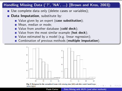
Handling Missing Data (’?’, ’NA’, ...) [Brown and Kros, 2003]:

Use complete data only (delete cases or variables);

Data Imputation, substitute by:

Value given by an expert (case substitution);Mean, median or mode;Value from another database (cold deck);Value from the most similar example (hot deck);Value estimated by a model (e.g. linear regression);Combination of previous methods (multiple imputation).


Non numerical variable remapping [Pyle, 1999]

Only numeric data can be fed into MLP, RBF, SVM, ...;

Binary attributes can be coded into 2 values (e.g. {-1, 1} or {0, 1});

Ordered attributes can be encoded by preserving the order (e.g. {low→ -1, medium → 0, high → 1});

Nominal (non-ordered with 3 or more classes) attributes:

One-of-NC remapping – use one binary variable per class (generic);Other remappings – requires domain knowledge (e.g. a state can becoded into 2 variables, the horizontal and vertical position in a 2Dmap).


Example of 1-of-NC remapping

x

bluered

yellow

Attribute color = {red, blue, yellow};With the linear mapping {red → -1 , blue → 0, yellow → 1} it isimpossible to describe X, which is orange (half red and half yellow);

With the 1-of-NC mapping {red →(1,0,0), blue→(0,1,0),yellow→(0,0,1)}, X could be represented by: (0.5,0,0.5).


Rescaling/Normalization [Sarle, 2002]

Several methods (MLP, SVM, ...) will improve learning if all Inputsare rescaled into the same range with a 0 mean:

x ′ = x−xs (standardization with mean 0 and standard deviation 1)

MLP: Outputs limited to the [0,1] range if logistic function is used([-1,1] if tanh):

y = (x−min)max−min (linear scaling with range [0, 1])


CRISP-DM phase 4 - Modeling

This stage involves selecting the learning models,estimation method, design strategy, building andassessing the models.

Estimation Method [Flexer, 1996]

Powerful learners (such as MLP and SVM) can easily overfit the data;

Thus, generalization capability needs to be assessed on unseen data;

This can be achieved using holdout or K-fold cross-validation;

Since the estimation method is stochastic (due to the randomtrain/test partition), R runs should be applied (common R values are5, 10, 20 or 30).


Holdout

Split the data into two exclusive sets, using random sampling:

training: used to fit the model (2/3);

test: used to measure the performance (1/3).

K-fold, works as above but uses rotation:

data is split into K exclusive folds of equal size (10-fold most used).

Test

1 2 3 4

1

1

2

2

2

3

3

3

4

4

41

1 2 3 4

Model 2

Model 3

Model 4

Model 1

Train


Design Strategy: initial configuration

Set initial model configuration details (e.g. number of hidden layersof MLP, SVM kernel type).

Common MLP setup (e.g. R tool):

Often, it is better to perform one classification/regression task permodel;

The number of input nodes is defined by the task;

Use of one hidden layer of H nodes with logistic functions;

Binary classification: one output node with logistic function;

Multi-class classification: NC output linear nodes (f (x) = x) andand the softmax function is used to transform these outputs into classprobabilities;

Regression: one linear output neuron.


Design Strategy: MLP training algorithm

Gradient-descent [Riedmiller, 1994]:

Backpropagation (BP) - most used, yet may be slow;

Other algorithms: Backpropagation with Momentum; QuickProp;RPROP; BGFS, Levenberg-Marquardt, ...

Evolutionary Computation [Rocha et al., 2007]

May overcome local minima problems;

Can be applied when no gradient information is available(reinforcement learning).


Design Strategy: local minima with MLP[Hastie et al., 2008]

The MLP weights are randomly initialized within small ranges (e.g.[-0.7;0.7]);

Each training may converge to a different (local) minima;

Solutions

Use of NR multiple trainings, selecting the MLP with lowest error;

Use an ensemble with NR MLPs, where the final output is given asthe average of the MLPs.


Design Strategy: model selection

Powerful learners (MLP, SVM) have several hyperparameters thatneed to be set/tuned;Such parameters can be set using: heuristic rules, simple grid-searchor more advanced optimization algorithms (e.g. EvolutionaryComputation) [Rocha et al., 2007];

Grid-Search

One (or more) parameters are scanned through a given range;

Range example for MLP hidden nodes: H ∈{0,2,4,. . .,20};Variants: two-level greedy grid-search (search at the first level andthen a second pass is taken, using a smaller range and step).

Error

Parameter value

Best value


Design Strategy: Variable Selection

Selection of the subset of relevant inputs. Why:

To facilitate data visualization/comprehension;Non relevant features/attributes will increase the model complexityand worst performances may be achieved;Ideally, model and (wrapper) variable selection should be performedsimultaneously;

Variable Selection methods [Witten and Frank, 2005]:

A priori knowledge (e.g. the use of experts);

Filter and Wrapper algorithms;

Trial-and-error blind search (e.g. test some subsets and select thesubset with the best performance);

Hill-climbing search (e.g. forward and backward selection);

Beam search (e.g. genetic algorithms).


Model Assessment: Classification Metrics

Confusion matrix [Kohavi and Provost, 1998]

Matches the predicted and actual values;

The 2× 2 confusion matrix:

↓ actual \ predicted → negative positivenegative TN FP

positive FN TP

Three accuracy measures can be defined:

the Accuracy = TN+TPTN+FP+FN+TP × 100 (%) (use if FP/FN costs are

equal);TPR or Sensitivity (Type II Error) = TP

FN+TP × 100 (%) ;

TNR or Specificity (Type I Error) ; = TNTN+FP × 100 (%)

The higher, the better (the ideal value is 100%);


Multi-class confusion matrix example [Cortez et al., 2009]:


Receiver Operating Characteristic (ROC) [Fawcett, 2006]

Shows the behavior of a 2 class classifier (y ∈ [0, 1]) when varying adecision parameter D ∈ [0, 1] (e.g. True if y > 0.5,D = 0.5);

The curve plots FPR = 1− TNR (x−axis) vs TPR (Sensitivity);

Global performance measured by the Area Under the Curve (AUC):

AUC =∫ 1

0 ROC dD (the perfect AUC value is 1.0).

0

1

1

D=1

D=0

Sensitivity

(TPR)

1−Specificity (FPR)

D=0.7

D=0.5

(AUC=0.5)Random classifier

Classifier(AUC=0.8) D=0.3


Model Assessment: Regression Metrics

y

i

global error

i

i

y

e

The error e is given by: e = y − y where y denotes the desired valueand the y estimated value (given by the model);


Given a dataset with the function pairs x1 → y1, · · · , xN → yN , we cancompute:

Error metrics

Mean Absolute Error/Deviation (MAE or MAD): MAD =PN

i=1|ei |N

Sum Squared Error (SSE): SSE =∑N

i=1 e2i

Mean Squared Error (MSE): MSE = SSEN

Root Mean Squared Error (RMSE): RMSE =√

MSE

Relative MAD (RMAD, scale independent):RMAD = MAD/MADbaseline × 100 (%), where baseline oftendenotes the average predictor.

Relative Root Mean Squared (RRMSE, scale independent):RRMSE = RMSE/RMSEbaseline × 100 (%)

The lower, the better (ideal value is 0).


Scatter plot: desired (x-axis) vs predicted (y-axis) values

Used to assess the prediction quality of a regression model;

The perfect fit is the diagonal line;

Civil engineering application example [Tinoco et al., 2009]:


Regression Error Characteristic (REC) curves[Bi and Bennett, 2003]

Used to compare several regression models;

The curve plots the error tolerance (absolute deviation, x-axis) versusthe percentage of points predicted within the tolerance (y -axis);


CRISP-DM phase 5 - Evaluation

The aim is to assess if the DM model meets thebusiness goals and if it is interesting.

Interestingness: does the model makes sense to thedomain experts and unveils useful or challenginginformation?

Business impact: by using such model, what is thegain achieved?


Business impact example: ROC Curve and benefit-cost analysis(FPR-TPR trade-off).


Interestingness: Explanatory Knowledge (MLP,RBF, SVM, ...), i.e. what has the model learned?

Sensitivity Analysis (SA) [Cortez and Embrechts, 2011]:

Allows a ranking of the inputs based on the amount of outputchanges when a given input is varied though its domain (i.e. with L levelsfor a 1-D SA).

Visualization techniques:

Input importances:

1 input SA - bar plot with the Ra importances, sorted from the highestto the lowest values.2 input SA - color matrix where a dark coloring, denoting aninteresting pair, was applied proportionally to the overall pair sensitivitymeasure.

Input Average Effect:

Variable Effect Characteristic Curve (VEC): to show the 1-D SAeffects of a given input variable on the model’s predictions.VEC Surface and Contour Plot: to show the 2-D SA effects.


Visualization of Input importance


Visualization of Input Effect: VEC curve (I)


Visualization of Input Effect: VEC curve (II)


Visualization of Input Effect: VEC surface andcontour


Extraction of rules from fitted models (MLP, SVM, ...)[Tickle et al., 1998, Setiono, 2003]

Pedagogical techniques extract the direct relationships between theinputs and outputs of the model;

By using a black-box point of view, less computation is required and asimpler set of rules may be achieved;

An example will be shown in the intensive care DM application.


CRISP-DM phase 6 - Deployment

The aim is to use the data mining results in the business or domainarea.

Deployment includes monitoring and maintenance: user feedback,checking if there have been changes in the environment (i.e. conceptdrift or shift) and if the DM model needs to be updated orredesigned;

The best model (MLP, SVM, ...) should be integrated into a friendlybusiness intelligence or decision support system;

The DM tool can export the best model into a standard format, suchas the predictive model markup language (PMML)[Grossman et al., 2002], and then the PMML model can be loadedinto a standalone program (e.g. written in C or Java).

The NN FAQ includes an extensive list of MLP software (e.g. writtenin C, C++ or Java) [Sarle, 2002].


rminer demo code: imports-85 UCI regression task

sample of rminer code:

# load datad=read.table(”imports-85.data”,sep=”,”,na.strings=”?”); d=na.omit(d)# model MLPNN=mining(V26 .,d,model=”mlpe”,Runs=5,method=c(”kfold”,3),search=”heuristic5”,f=”s”)# scatter plotmgraph(NN,graph=”RSC”,main=”MLP”,baseline=TRUE,Grid=TRUE)


Some DM application examples

Binary Classification (SVM): Spam Telescope Miner R&D project

Spam email detection using network-level properties[Cortez et al., 2010];


Binary Classification (SVM): Bank Marketing Data

The data is related with direct marketing campaigns (phone calls) ofa Portuguese banking institution. The classification goal is to predictif the client will subscribe a term deposit (variable y)[Moro et al., 2011];


Regression (MLP): Internet Traffic Forecasting [Cortez et al., 2012]

Hourly forecast of a private European ISP Internet traffic:


Ordinal Classification/Regression (MLP, SVM): Modeling winequality [Cortez et al., 2009]

Predicting vinho verde wine preferences based on physicochemicalproperties (e.g. pH, alcohol):


Detailed Application Example: Intensive CareMedicine (Classification) [Silva et al., 2008]


1. Business Understanding:

Intensive Care Units (ICU)

In the last decades, a worldwide expansion occurred in thenumber of Intensive Care Units (ICUs);

Scoring the severity of illness has become a daily practice, withseveral metrics available (e.g. SAPS II, SOFA);

These scores have been used to improve the quality of intensivecare and guide local planning of resources;

Most of these scores are static (i.e. use data collected only onthe first day);

More recently, dynamic (or daily updated) scores have beendesigned, such as the sequential organ failure assessment(SOFA).


Motivation (I)

SOFA score

Six organ systems (respiratory, coagulation, hepatic,cardiovascular, neurological and renal) are scored from 0 to 4,according to the degree of failure;

Expert-driven score: a panel of experts selected a set of variablesand rules based on their personal opinions;

Widely used in European ICUs;

Issues not yet solved:

It is not clear how many daily times some variables (e.g.platelets, bilirubin) should be measured;

No risk (i.e. probability) is provided for the outcome of interest(i.e. organ failure).


Motivation (II)

Bedside Monitoring Data

Universal and routinely registered during patient ICU stay;

The relationships within these biometrics are complex, nonlinear andnot fully understood;

Monitoring analysis is not standardized and mainly relies on thephysicians knowledge and experience;

The laboratory data usually depend on previous physiologicalimpairments, thus using only biometric data should allow a moreadequate evaluation and early therapeutic intervention

Yet, an high amount of data available (several biometrics with toomuch detail), generating alarms that need to be interpreted;

In previous work [Silva et al., 2006], it has been shown that adverseevents of four biometrics have an impact on the mortality outcomeof ICU patients.


Aim

The main goal is to explore the impact of the adverse events,during the last 24h, on the current day organ risk condition (i.e.normal, dysfunction or failure);

As a secondary goal, two DM techniques (i.e. Logistic Regressionand NN) are evaluated and compared.


2. Data Understanding

Data Collection

A EURICUS II derived database was adopted, with records takenfrom 9 EU countries and 42 ICUs, during 10 months, from 1998 until1999;

Data manually collected by the nursing staff (every hour);

The registered data was submitted to a double check, using bothlocal (i.e. ICU) and central levels (i.e. Health Services Research Unitof the Groningen University Hospital, the Netherlands);

The latter unit was used to gather the full database.


3. Data Preparation

Preprocessing

After a consult with ICU specialists, the patients with age lower than18, burned or bypass surgery were discarded;

Also, the last day of stay data entries were discarded, since the SOFAscore is only defined for a 24h time frame and several of thesepatients were discharged earlier;

Final database with 25215 daily records taken from 4425 patients.


Protocol for the out of range physiologicmeasurements

BP SpO2 HR URNormal Range 90− 180mmHg ≥ 90% 60− 120bpm ≥ 30ml/hEventa ≥ 10min. ≥ 10min. ≥ 10min. ≥ 1h

Eventb ≥ 10min. in 30min. ≥ 10min. in 30min. ≥ 10min. in 30min. –Critical Eventa ≥ 1h ≥ 1h ≥ 1h ≥ 2h

Critical Eventb ≥ 1h in 2h ≥ 1h in 2h ≥ 1h in 2h –Critical Eventc < 60mmHg < 80% < 30bpm ∨ > 180bpm ≤ 10ml/h

BP - blood pressure, HR - heart rate, SpO2 - pulse oximeter oxygensaturation, UR - urine output.

a Defined when continuously out of range.b Defined when intermittently out of range.c Defined anytime.


The intensive care variables

Attribute Description Min Max Meana

admtype admission type Categoricalb

admfrom admission origin Categoricalc

SAPS II SAPS II score 0 118 40.9±16.4age age of the patient 18 100 62.5±18.2NBP daily number of blood pressure events 0 24 0.8±1.9NHR daily number of heart rate events 0 24 0.6±2.3NSpO2 daily number of oxygen events 0 24 0.4±1.8NUR daily number of urine events 0 24 1.0±3.0NCRBP daily number of critical blood pressure events 0 10 0.3±0.7NCRHR daily number of critical heart rate events 0 10 0.2±0.6NCRSpO2 daily number of critical oxygen events 0 6 0.1±0.4NCRUR daily number of critical urine events 0 7 0.4±0.8TCRBP time of critical blood pressure events (% of 24h) 0 24.7 0.8±2.7TCRHR time of critical heart rate events (% of 24h) 0 24.7 1.0±3.4TCRSpO2 time of critical oxygen events (% of 24h) 0 24.7 0.4±2.1TCRUR time of critical urine events (% of 24h) 0 24.7 1.6±4.5

a mean and sample standard deviation.b 1 - unscheduled surgery, 2 - scheduled surgery, 3 - medical.c 1 - operating theatre, 2 - recovery room, 3 - emergency room, 4 - general ward,

5 - other ICU, 6 - other hospital, 7 - other sources.


Boxplots of Critical Events per Renal Condition


Organ condition prevalence (histograms)

Respiratory

0 1 2 3 4

0200

0400

0600

0800

0

Normal

Dysfunction

Failure

Coagulation

0 1 2 3 40

5000

10000

15000

Normal

Dysfunction

Failure

Hepatic

0 1 2 3 4

0500

0100

00150

00200

00 Normal

Dysfunction

Failure

Cardiovascular

0 1 2 3 4

0500

0100

00150

00

Normal

DysfunctionFailure

Neurological

0 1 2 3 4

0500

0100

00150

00 Normal

DysfunctionFailure

Renal

0 1 2 3 40

5000

10000

15000

Normal

Dysfunction

Failure


4. Modeling

Multinomial Logistic Regression (MLR)

The logistic regression is the most popular model within ICUphysicians;

The MLR is the extension to multi-class tasks:

pj =exp(ηj x)PNC

k=1 exp(ηkx)

ηj(x) =∑I

i=1 βj ,ixi

(1)

where βj ,0, . . . , βj ,I denotes the parameters of the model, andx1, . . . , xI the dependent variables;

This model requires that ηk(x) ≡ 0 for one ck ∈ C (the baselinegroup) and this assures that

∑NCj=1 pj = 1;


Neural Network (NN)

Fully connected MLPs with bias connections, one hidden layer of Hnodes and logistic activation functions;

Linear function used at the NC output nodes;

The final probability is given by:

pj =exp(yj )PNC

k=1 exp(yk )(softmax function)

yi = wi,0 +∑I+H

m=I+1 f (∑I

n=1 xnwm,n + wm,0)wi,n

(2)

where yi is the output of the network for the node i ; f = 11+exp(−x) is

the logistic function; I represents the number of input neurons; wd ,s

the weight of the connection between nodes s and d ; and wd ,0 is thebias.


MLR vs NN

/Σ

ΣΣ

Σ

Σ Σ

Σ

Σ

ΣΣ

exp

exp

exp

p

p

p

normal

dysfunction

failure

softmax

softmax

softmax

output node

SAPSII

age sum

weights

1

1+ e−sum

sum 1

1+ e−sum

dysfunctionsoftmax

coefficient

SAPSII

age

softmax pfailure

pnormal

probability hidden node probabilitysoftmax

p


Feature and Model selection

A backward feature selection based on the sensitivity analysis wasused;

H (hidden nodes) fixed to the median of the grid range during thefeature selection phase;

After feature selection, the number of hidden nodes (H) was tunedusing a simple grid search H ∈ {2, 4, 6, 8, 10};For both feature and H searches, the training data is randomly splitinto training (66.6%) and validation (33.3%) sets;

The model with the lowest validation error is selected and the finalmodel is retrained with all available data.


Experiments

The R (statistical tool, open source) environment and rminer library(nnet and kernlab packages) was used in all experiments[Cortez, 2010];

Training with the BGFS algorithm (quasi-newton method), set tomaximize the likelihood;

Continuous inputs were scaled into a zero mean and one standarddeviation range; the nominal inputs were encoded into 1-of-NC binaryvariables; Admtype example: 1 → (1, 0, 0); 2 → (0, 1, 0); and3 → (0, 0, 1).

To compare the learning models, 20 runs of a 5-fold cross-validation[Kohavi, 1995] were executed (in a total of 20× 5 simulations).

Paired statistical comparison using the Mann-Whitney non-parametrictest at the 95% confidence level.


5. Evaluation

Metrics:

Discrimination: AUC of ROC

Multi-class problem: one ROC per class and then compute a globalAUC value weighted by the class prevalence;

Calibration: Brier Score

The ROC measures the discrimination power, but in medicine it isalso important to have a good calibration: the predictions should beclose to the true probabilities of the event;

Calibration will be measured using the Brier score;

The Brier Score (also known as MSE) for a two-class scenario is:Brier(cj) = 1

N

∑Ni=1(pi

j − pij )

2

Inspired in the multi-class AUC metric, the global Brier score isdefined as: BrierGlobal =

∑ci∈C Brier(ci ) · prev(ci )


Discrimination Results (values of AUC>70% are inbold)

Normal Dysfunction Failure GlobalOrgan MLR NN MLR NN MLR NN MLR NNrespiratory 67.2 69.5 59.2 61.0 65.6 68.9 63.6 66.0coagulation 63.6 65.5 60.1 62.0 72.6 73.9 63.3 65.1hepatic 64.7 66.7 62.5 64.2 72.6 76.0 64.6 66.6cardiovascular 67.9 71.2 63.8 65.6 67.3 71.0 67.1 70.2neurological 70.0 72.1 58.8 61.2 74.7 76.7 68.8 70.9renal 69.4 70.7 66.0 66.8 73.5 76.1 69.1 70.4Average 67.1 69.3 61.7 63.5 71.0 73.8 66.1 68.2

In all cases, the NN/MLR differences are significant;

The median number of H is 8 for all organs (except neurologicalwhere H=10);

The feature selection discarded an average of two attributes.


Calibration Results (Brier score values)

Normal Dysfunction Failure GlobalOrgan MLR NN MLR NN MLR NN MLR NNrespiratory 0.213 0.204 0.233 0.230 0.171 0.166 0.211 0.205coagulation 0.173 0.171 0.155 0.154 0.038 0.038 0.134 0.133hepatic 0.132 0.130 0.116 0.116 0.026 0.025 0.101 0.100cardiovascular 0.205 0.197 0.132 0.130 0.138 0.133 0.160 0.155neurological 0.208 0.202 0.153 0.151 0.136 0.132 0.169 0.165renal 0.182 0.179 0.155 0.155 0.065 0.063 0.144 0.142Average 0.185 0.181 0.157 0.156 0.096 0.093 0.153 0.150

Values in bold denote statistical significance when compared with MLR.


Results: ROC (renal failure) and REC (respiratoryfailure)

Renal: failure

0 0.2 0.4 0.6 0.8 1

00.

20.

40.

60.

81 Respiratory: failure

020

4060

8010

0

0 0.2 0.4 0.6 0.8 1


Input Relevance (NN)

Organ admtype admfrom SAPS II age BP? HR? SpO2? UR?

respiratory 16.8 7.8 15.1 10.0 19.9 8.1 17.1 5.2coagulation 30.9 10.8 12.7 7.0 7.5 2.6 18.1 10.4hepatic 23.1 7.8 12.1 10.8 9.1 5.1 17.0 15.0cardiovascular 14.1 17.3 16.5 12.8 9.8 9.6 13.4 6.5neurological 31.2 10.2 15.6 7.5 17.3 3.5 10.4 4.3renal 2.3 13.6 26.6 9.9 5.1 6.4 19.8 16.3Average 19.7 11.3 16.4 9.7 11.4 5.9 16.0 9.6

? – All attributes related to the variable where summed (number of events, critical events andthe time).


Knowledge extraction (Decision Tree example forthe renal organ)

SAPSII<74NUR<15

NHR<2

dysfunc.NCRHR>0 SAPSII<47

admtype=3dysfunc.SAPSII<93

dysfunc.

failure

failure age<62

false

admfrom=5,6

split nodeleave

TCRUR<13.8true

false

false

true

normal

normalnormal

normal

normal

normal


6. Deployment (still future work)

This approach (and others) is being tested a real environment with anon-line learning (pilot project INTCare, Hospital S. Antonio, Porto,Portugal;


Conclusions

A data-driven analysis was performed on a large ICU database,with an emphasis on the use of daily adverse events, taken fromfour commonly monitored biometrics;

The obtained results show that adverse events are importantintermediate outcomes;

It is possible to use DM methods to get knowledge from easyobtainable data, thus opening room for the development ofintelligent clinical alarm monitoring;

With the same inputs, the NNs outperform the LogisticRegression;


”And Now for SomethingCompletely Different”: niceartificial life MLP demo


Bi, J. and Bennett, K. (2003).Regression Error Characteristic curves.In Fawcett, T. and Mishra, N., editors, Proceedings of 20th Int. Conf.on Machine Learning (ICML), Washington DC, USA, AAAI Press.

Bishop, C. (1995).Neural Networks for Pattern Recognition.Oxford University Press.

Brown, M. and Kros, J. (2003).Data mining and the impact of missing data.Industrial Management & Data Systems, 103(8):611–621.

Chapman, P., Clinton, J., Kerber, R., Khabaza, T., Reinartz, T.,Shearer, C., and Wirth, R. (2000).CRISP-DM 1.0: Step-by-step data mining guide.CRISP-DM consortium.

Cortez, P. (2010).Data Mining with Neural Networks and Support Vector Machinesusing the R/rminer Tool.


In Perner, P., editor, Advances in Data Mining – Applications andTheoretical Aspects, 10th Industrial Conference on Data Mining,pages 572–583, Berlin, Germany. LNAI 6171, Springer.

Cortez, P. (2012).Data Mining with Multilayer Perceptrons and Support VectorMachines, chapter 2, pages 9–25.Springer.

Cortez, P., Cerdeira, A., Almeida, F., Matos, T., and Reis, J. (2009).Modeling wine preferences by data mining from physicochemicalproperties.Decision Support Systems, 47(4):547–553.

Cortez, P., Correia, A., Sousa, P., Rocha, M., and Rio, M. (2010).Spam Email Filtering Using Network-Level Properties.In Perner, P., editor, Advances in Data Mining – Applications andTheoretical Aspects, 10th Industrial Conference on Data Mining,pages 476–489, Berlin, Germany. LNAI 6171, Springer.

Cortez, P. and Embrechts, M. (2011).


Opening black box data mining models using sensitivity analysis.In IEEE Symposium Series in Computational Intelligence 2011 (SSCI2011), pages 341–348, Paris, France.

Cortez, P., Rio, M., Rocha, M., and Sousa, P. (2012).Multi-scale internet traffic forecasting using neural networks and timeseries methods.Expert Systems, 29(2):143–155.

Fawcett, T. (2006).An introduction to ROC analysis.Pattern Recognition Letters, 27:861–874.

Fayyad, U., Piatetsky-Shapiro, G., and Smyth, P. (1996).Advances in Knowledge Discovery and Data Mining.MIT Press.

Flexer, A. (1996).Statistical Evaluation of Neural Networks Experiments: MinimumRequirements and Current Practice.


In Proceedings of the 13th European Meeting on Cybernetics andSystems Research, volume 2, pages 1005–1008, Vienna, Austria.

Grossman, R., Hornick, M., and Meyer, G. (2002).Data Mining Standards Initiatives.Communications of ACM, 45(8):59–61.

Hastie, T., Tibshirani, R., and Friedman, J. (2008).The Elements of Statistical Learning: Data Mining, Inference, andPrediction.Springer-Verlag, NY, USA, 2nd edition.

Haykin, S. (2009).Neural networks and learning machines.Prentice Hall.

Kohavi, R. (1995).A Study of Cross-Validation and Bootstrap for Accuracy Estimationand Model Selection.


In Proceedings of the International Joint Conference on ArtificialIntelligence (IJCAI), Volume 2, Montreal, Quebec, Canada, MorganKaufmann.

Kohavi, R. and Provost, F. (1998).Glossary of Terms.Machine Learning, 30(2/3):271–274.

Moro, S., Laureano, R., and Cortez, P. (2011).Using data mining for bank direct marketing: an application of thecrisp-dm methodology.In European Simulation and Modelling Conference - ESM’2011, pages117–121. Eurosis.

Piatetsky-Shapiro, G. (2010).Software Suites for Data Mining, Analytics, and Knowledge Discovery.http://www.kdnuggets.com/software/suites.html.

Piatetsky-Shapiro, G. (2012).Analytics, Data mining, Big Data software used.


http://www.kdnuggets.com/polls/2012/analytics-data-mining-big-data-software.html.

Pyle, D. (1999).Data Preparation for Data Mining.Morgan Kaufmann, S. Francisco CA, USA.

Riedmiller, M. (1994).Supervised Learning in Multilayer Perceptrons - from Backpropagationto Adaptive Learning Techniques.Computer Standards and Interfaces, 16.

Rocha, M., Cortez, P., and Neves, J. (2007).Evolution of Neural Networks for Classification and Regression.Neurocomputing, 70:2809–2816.

Sarle, W. (2002).Neural Network Frequently Asked Questions.Available at: ftp://ftp.sas.com/pub/neural/FAQ.html.

Setiono, R. (2003).


Techniques for Extracting Classification and Regression Rules fromArtificial Neural Networks.In Fogel, D. and Robinson, C., editors, Computational Intelligence:The Experts Speak, pages 99–114. Piscataway, NY, USA, IEEE.

Silva, A., Cortez, P., Santos, M. F., Gomes, L., and Neves, J. (2006).Mortality assessment in intensive care units via adverse events usingartificial neural networks.Artificial Intelligence in Medicine, 36:223–234.

Silva, A., Cortez, P., Santos, M. F., Gomes, L., and Neves, J. (2008).Rating organ failure via adverse events using data mining in theintensive care unit.Artificial Intelligence in Medicine, 43(3):179–193.

Tickle, A., Andrews, R., Golea, M., and Diederich, J. (1998).The Truth Will Come to Light: Directions and Challenges inExtracting the Knowledge Embedded Within Trained Artificial NeuralNetworks.IEEE Transactions on Neural Networks, 9(6):1057–1068.


Tinoco, J., Correia, A., and Cortez, P. (2009).A Data Mining Approach for Jet Grouting Uniaxial CompressiveStrength Prediction.In World Congress on Nature and Biologically Inspired Computing(NaBIC’09), pages 553–558, Coimbatore, India. IEEE.

Turban, E., Sharda, R., and Delen, D. (2010).Decision Support and Business Intelligence Systems.Prentice Hall, 9th edition.

Witten, I. and Frank, E. (2005).Data Mining: Practical Machine Learning Tools and Techniques withJava Implementations.Morgan Kaufmann, San Francisco, CA.


data mining with mlps (and other methods) · great emphasis in using expert systems ... paulo...

Documents