JMARVolume Ftve

Fall 1993

(D2.Economic Implications of Single Cost

Driver Systems

Rajiv D. BankerUniversity of Minnesota

andGordon Potter

University of Minnesota

Abstract: We subject claims about the benefits of activity-based costing sys-tems to the scrutiny of analytical models incorporating rational behavior by us-ers of product costing systems. We find that a monopolist Is almost always strictlybetter off using multiple cost drivers as in an activity-based costing (ABC) sys-tem even when the system makes measurement errors in assigning overheadcosts to activities. More importantly, we show that this result replicates for firmscompeting in an oligopoly when the cost and demand parameters are in steadystate. The firms are strictly better off using a direct labor based single cost driver(SCO) system, however, if the demand for the overcosted labor intensive prod-uct is expected to grow sufficiently relative to the demand for the undercostedsetup intensive product. This suggests that, facing imperfect competition, it issometimes optimal for firms to persist in using a single cost driver system ratherthan switching to an activity-based cost system.

• u> I. INTRODUCTION /

The recent management accounting literature provides several casestudies of multi-product Rrms whose product costs are distorted becausethey allocate overhead costs to products on the basis of a single volume-related variable. Johnson and Kaplan [19871 report that most of the firmsthat they have personally studied use simple cost accounting systems thatassign overhead costs to products based on the direct labor hours expendedon each product. Cooper and Kaplan [19871 describe three multi-productfirms with complex manufacturing processes that rely mainly on directlabor hours to allocate overhead costs to products. They document howthe apportionment of (long term) variable overhead costs on the basis of asingle cost driver led these firms to overcost some high-volume productsand undercost most low-volume products. Cooper [1987] argues that suchobsolete single cost driver based systems often lead to improper pricingand distort "the strategy selected by the flrm....tempting management tofocus incorrectly on low-volume, specialty business." Shank andGovlndarajan [1988] echo this, stating 'Volume-based costing can seriously

Helpful comments and suggestions Jixym an anonymous referee and seminar partici-pants at University ofCaltfornia (Berkeley). UniversUy of California (Los Angeles).Michigan State Uniuersity, University of Minnesota. Rice University. San Diego StateUniversity. Stanford University. UniversUy of Wisconsin (Madison), and the 1991Annual Management AccountiT^ Research Conference are gratefully acknowledged.

16 JcHimal of Management Accounting Research Fall 1993

distort the way a firm ... assesses the profit impact of its pricing and prod-uct emphasis decision." This assumption that It is sub-optimal for firms topersist In the use of single cost driver systems seems to be an axiom in thecost driver literature, but it has received little attention in the analyticalmanagement accounting literature.

A recent survey of 566 controllers by the National Association of Ac-countants [Schiff, 1991] indicated that 11 percent have implemented anactivity-based costing (ABC) system. 19 percent are considering it and 70percent of the firms are not currently considering switching to an activity-based costing system. Miller and Kim (1990] find that 22 percent of the2(X) large manufacturing firms they surveyed used ABC—but it was thesecond least effective action in terms of 1988-89 payoff. While this repre-sents a faster rate of adoption than that observed for previous innovationsin management accounting, such as the use of discounted cash fiow analysisfor capital budgeting, it Is not apparent that aU firms in all industries per-ceive that the benefits from using an ABC system outweigh the costs ofimplementing and operating it.

One explanation for the continued use of single cost driver (SCD) sys-tems may be the high cost of switching to an ABC system that recognizesmultiple cost drivers. Such costs may include personnel, consulting, train-ing and software costs for installing an ABC system, as well as organiza-tional costs resulting from consequent realignment of strategies espousedby managers based on information provided by SCD systems. Costs of com-puterizing and operating complex multi-purpose cost systems, however,have declined sharply in recent years. In any case, such costs must beweighed against the presumed benefits from a multiple cost driver sys-tem.^ In this paper therefore, we ask the questions whether and to whatextent a firm will benefit more if it switches from a SCD to an ABC systemfor its product mix decisions. We also identify conditions under which theuse of a SCD system leads to higher expected profits than an ABC systemeven when the costs of implementing an ABC system are negligible.

We consider two different possibilities. First, we recognize that a mul-tiple cost driver system may introduce errors because precise identifica-tion of the overhead costs associated with specific cost drivers may not bepossible. Such accounting inaccuracies introduced in multiple cost driversystems need to be traded off against the imprecision resulting from thepooling of all overhead costs into a single cost driver system. Second, we

'An Important empirical question Is whether overhead costs depend on activity variablesother than volume-related variables like direct labor. Cooper [1987], Johnson and Kaplan11987], Miller and Vollman (19851 and others assert that a significant portion of manufacturingoverheads varies with transactions such as setups, purchase orders, engineering changeorders and material movements. Using a sample of 37 plants owned by one firm, Foster andGupta I1990I, however, find that manufacturing overhead is more frequently significantlycorrelated with volume-related drivers than complexity or efndency-related drivers. Bankerand Johnston 11993] ftnd a similar highly significant relation between overheads and volumemeasures for a sample of airline firms, but they also find several operating strategy variablesto be significant drivers of overhead costs. Using a sample of 31 plants from firms in theelectronics, machinery and automobile components industries. Banker et al. 11992) confirmthe high correlation between manufacturing overheads and direct labor, but they find thatcomplexity variables representing transactions Identified by Miller and Vollmann are alsosignificant. This empirical question is important because If cost drivers other than directlabor-type volume measures are Insignificant, then any benefits from switching from a singlevolume-based cost driver system are likely to be minimal.

Banker and Potter 17

recognize the possibility that the implications of product costs for a firm'spricing and product mix decisions may be quite different when it competesin an oligopoly than when it operates as a monopolist. In particular, wenote that explicit collusion between firms is precluded by anti-trust stat-ute in most oligopolistic environments, and therefore, we examine whetherproduct mix decisions based on distorted product costs can lead to anequilibrium that is more favorable to all the firms in an oligopoly than thatattained when such decisions are based on accurate product costs.^

A standard result in oligopoly theory is that competitive prices are strictlyless than collusive prices; collusive prices yield higher profits for all ilrms.Equilibrium prices are increasing in the perceived product costs. An obvi-ous result, therefore, is that all firms are better off if they commit to usingcost systems that inflate aU product costs by some positive amount.^ Suchan observation, however, has little descriptive value in comparing actualproduct costing systems that are institutionally constrained to base prod-uct cost estimates on actual costs. That is, in SCD, ABC and most com-mon cost accounting systems, if the cost of one product is overstated thenit must be ofTset by understated costs for some other products. It is nolonger obvious, therefore, that distortion of product costs increases ex-pected profits. This analytical tension from both over- and understatementof product costs makes the problem of evaluating the expected profit im-pact of product costing systems interesting, and forms the focus of ourpaper.

The remainder of this paper has the following structure. The next sec-tion develops our basic model for a monopolist flrm producing two prod-ucts, and compares an imperfect activity-based costing system with a singlecost driver system. Section III extends our model to identify conditionsunder which the use of a single cost driver based system by all firms in anoligopoly dominates their use of a perfect activity-based costing system.Section IV concludes the paper.

n. PRODUCT MIX PROBLEM IN A MONOPOLYWe begin by considering a monopolist firm that produces two prod-

ucts. J= 1,2. The true expected (long term) variable cost c, fora unit of prod-uct j is represented as the sum of the expected direct cost v, and the ex-pected (long term) variable overhead h,:

Cj =Vj +hj • ( I )

where Cj = total expected (long term) variable cost per unit of product jVj = expected direct cost per unit of product Jhj =expected (long term) variable overhead cost per unit of product j

The activity-based costing literature [e.g.. Cooper and Kaplan, 1987]prescribes the use of long term variable costs for evaluating product profit-ability.'* In our model, the total actual (long term) variable overhead costs

A possibility that we do not consider in this paper Is whether the finer information providedby activity analysis is valuable for monitoring and Ineentive purposes.

^Alles 119911 also discovered this same result.^Banker and Hughes |19911 show that expected equilibrium product prices in imperfectly

competitive markets are functions of their corresponding "long term variable" costs.

18 Journal of Management Accounting ResearcK Fall 1993

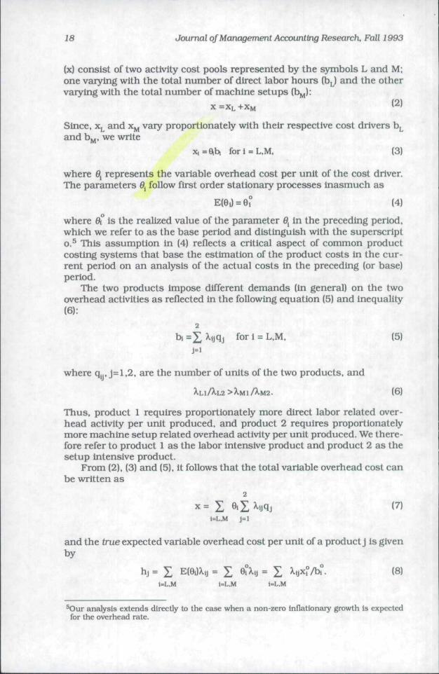
(x) consist of two activity cost pools represented by the symbols L and M;one varying with the total number of direct labor hours (bj and the othervaiying with the total number of machine setups (b^):

X = X L + X M

since, x^ and x^ vary proportionately with their respective cost drivers b^and b^. we write

x,=e,b, fori=L,M, (3)

where 9^ represents the variable overhead cost per unit of the cost driver.The parameters 6^ follow first order stationary processes inasmuch as

E(ei) = 6° (4)

where ft Is the realized value of the parameter 6^ in the preceding period,which we refer to as the base period and distinguish with the superscripto. This assumption in (4) reflects a critical aspect of common productcosting systems that base the estimation ofthe product costs in the cur-rent period on an analysis of the actual costs in the preceding (or base)period.

The two products impose different demands (in general) on the twooverhead activities as reflected in the following equation (5) and inequality(6):

2for i = L,M, (5)

where q,,. J=1.2, are the number of units ofthe two products, and

>XMI AM2- (6)

Thus, product 1 requires proportionately more direct labor related over-head activity per unit produced, and product 2 requires proportionatelymore machine setup related overhead activity per unit produced. We there-fore refer to product 1 as the labor intensive product and product 2 as thesetup Intensive product.

From (2), (3) and (5), it follows that the total variable overhead cost canbe written as

1=L.M J=l

and the true expected variable overhead cost per unit of a product j Is givenby

hj = X E(et)Xij = X ^^^i = S hix^/^. (8)f-L.M 1-L.M i-L.M

analysis extends directly to the case when a non-zero inflationary growth Is expectedfor the overhead rate.

Banker and Potter ifl

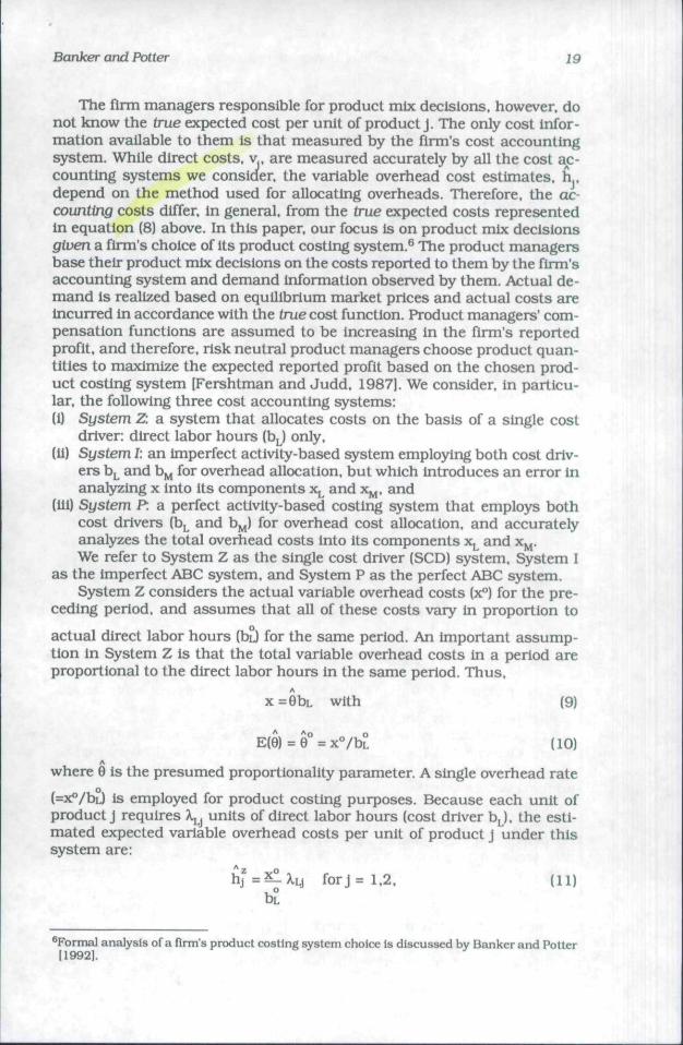
The firm managers responsible for product mix decisions, however, donot know the true expected cost per unit of product J. The only cost infor-mation available to them is that measured by the firm's cost accountingsystem. While direct costs, v,. are measured accurately by all the cost a c-countlng systems we consider, the variable overhead cost estimates, h,,depend on the method used for allocating overheads. Therefore, the ac-counting costs differ, in general, from the true expected costs representedin equation (8) above. In this paper, our focus is on product mix decisionsgiven a firm's choice of its product costing system.^ The product managersbase their product mix decisions on the costs reported to them by the firm'saccounting system and demand information observed by them. Actual de-mand is realized based on equilibrium market prices and actual costs areincurred in accordance with the true cost function. Product managers' com-pensation functions are assumed to be increasing in the firm's reportedprofit, and therefore, risk neutral product managers choose product quan-tities to maximize the expected reported profit based on the chosen prod-uct costing system [Fershtman and Judd, 1987], We consider, in particu-lar, the following three cost accounting systems:(i) System Z: a system that allocates costs on the basis of a single cost

driver: direct labor hours [hj only,(ii) System /: an imperfect activity-based system employing both cost driv-

ers b^ and b^ for overhead allocation, but which introduces an error inanalyzing x into its components x^ and x^. and

(iii) System R a perfect activity-based costing system that employs bothcost drivers (bL and b, ,) for overhead cost allocation, and accuratelyanalyzes the total overhead costs into its components x^^ and x^.We refer to System Z as the single cost driver (SCD) system. System I

as the imperfect ABC system, and System P as the perfect ABC system.System Z considers the actual variable overhead costs (x°) for the pre-

ceding period, and assumes that all of these costs vary in proportion to

actual direct labor hours (bU for the same period. An important assump-tion in System Z is that the total variable overhead costs in a period areproportional to the direct labor hours in the same period. Thus.

x=ebL with (9)

" (10)

where 9 is the presumed proportionality parameter. A single overhead rate

(=x°/bL) is employed for product costing purposes. Because each unit ofproduct j requires X j units of direct labor hours (cost driver b j , the esti-mated expected variable overhead costs per unit of product j under thissystem are:

hi=^X^ forj= 1,2, (11)

^Formal analysis of a firm's product costing system choice Is discussed by Banker and Potter[19921.

20 Journal of Management Acxx>imting ResearcK Fall 1993

where the superscript o. as before, represents the base period. It also fol-

lows immediately from (6) that product 1 is overcosted (hi > hj) and prod-

uct 2 is undercosted (h2 < hj).System I divides the total variable overhead costs into two activity-based

cost pools. While the total variable overhead costs (x°) for the base periodare observed accurately, we allow for the possibility that the division of thecosts into two pools introduces some measurement error [e°] randomlydistributed with mean e° and variance o^ <«*. Thus, the observed overhead

A

cost pools Xi, i = L.M, are equal to:XL - XL - e li^J

XM — X| + e I loj

The basic assumption in System I is that the observed overhead costsin each pool are proportional to the corresponding cost driver, so that

x= J e,bi with (14)1=L.M

E(6i) = 9i = Xj /bi for i = L,M. (15)

A

where 6, are the presumed proportionality parameters. Thus, two overheadcost rates (= xf'A)!, i = L.M) are employed for product costing purposes.This imperfect activity based costing system then estimates unit variableoverhead costs as:

hj = 21 ^ijx,/bi forj = 1,2. (16)

System I undercosts the labor intensive product 1 (and overcosts the setup

intensive product 2) if and only if e° > 0. Product managers observe only hj

if System I is in place, they do not know the actual e°. e° or of.The perfect activity based costing system. System P, operates just like

System I except that the actual measurement error e° is always equal tozero in this case, and hence it provides unbiased estimates of the truevariable overhead costs.

While the cost structures outlined above are abstractions, they cap-ture the most important difference between direct labor based (System Z)and activity-based (Systems I and P) costing systems. The true overheadcosts are driven by more than one factor, and this fact is captured accu-rately only by System P. System I reflects the potential for measurementerror in an accounting ^^tem that assigns costs to multiple overhead pools,and System Z reflects the observed phenomenon of firms allocating over-head costs to products based on direct labor alone.

The inverse demand functions for the monopolist firm in the two prod-uct markets are represented by the linear forms:

Banker and Potter 21

forJ = 1.2. (17)where Pj is the price of product J. Oj and pj > 0 are the estimated param-eters of the inverse demand function, and e, reflects the residual uncer-tainty when estimating the demand relation.^ It is also assumed implicitlyin the above expression that the values of q, are constrained to ensure thatp, remains positive.

The following equation then specifies the expected reported profit whena cost accounting system s. s = Z.I.P. is employed, and the product mixrepresented by the quantities q, and qj is chosen:

qj-f fors = Z.I.P. (18)

where f > 0 represents fixed costs and hj is the estimated unit variableoverhead cost for product j .

The flrm managers with the delegated responsibility for product mixdecisions, choose q, to maximize the expected reported profit in equation(18). The first order optimality condition yields the following perceived op-timal quantity:^

qj = (ttj -vj -hJ)/2Pj for s = Z.I.P.

The true expected profit when the quantities qj* are chosen is then givenby:

2

E(7c* ) = £ (ttj - pjqj - Vj - hj) q; - f for s = Z.I.P. ,, \m

Note that whereas the optimal quantity in (19) is based on the perceivedA

costs hj. the term hj in (20) represents the true expected unit variable over-"p

head costs. (In particular, of course, hj = h, because the perfect activitybased costing system yields unbiased estimates.)

Comparing the optimal expected profit under System Z or System Iwith that under System P. we obtain for s = Z.I.

i"4ft " '

hj'-hi) /4j3j > 0

-hJ) - 2(aj - +hj)]

(21)

'The residual G. IS assumed to be statlsUcally Independent of the corresponding randomvariable representing the uncertainty remaining when estimating the (long term) variablecosts of product J.

*rhe second order conditions for maximization are also satisfied, so that the first order condition

as in £19) always characterizes the optimal solution for a|-vj-hj'2 0.

22 Journal of Management Accounting ResearcK Fall 1993

We formalize this relation in the following:Proposition Ka): The monopolist firm is always strictly better off basingits product quantity choice on costs generated by System P rather thaneither System I or System Z.Next, we employ the expressions in (3), (8), (11) and (16) to compare the

estimated unit variable overhead costs hj. s=Z.I, J=l,2, with the true costshj. Thus

(22)

- h j = -

_ X M J

obM.

3

^4 ^MJ (23)

Therefore, using (21) and (23), and taking expectation over e°, we ob-tain

J [ ?'] [^ M > 0 (24)

Thus, the expected value of the imperfect ABC system is strictly de-creasing in the aprtorfbias e° and noise o?. While this result is intuitive fora single decision maker, we shali see in the next section that it holds in anoligopolistic environment only under specific conditions.

The difference between the optimal expected profits under the imper-fect activity based costing system. System I. and the direct labor basedsystem. System Z, is given by:

£ [(;,) ] \ \ (25)

The difference is positive provided (x , )^ - I e° I ><^. Thus, we haveProposition 1 (b): The monopolist firm is strictly better off using the costestimates generated by System I rather than by System Z if and only ifthe variance of the measurement error e° is less than the difference inthe squares of the true variable overhead cost x^ and the a priori biase°.

A

Since the measured overhead cost pool amount xy in (13) cannot benegative, we have - e° < x^. Therefore, a System I that systematically in-troduces a bias e° with certainty (< = 0) is preferred over System Z unlessthe bias is so large that it doubles the costs assigned to the overhead poolM. Such large bias might occur if cost pool x^ is veiy large relative to x^.Intuitively, System Z can be thought of as committing a 100 percent mea-surement error (e° = - x^) with certainty (ai = 0). and therefore it is strictly

Banker and Fitter 23

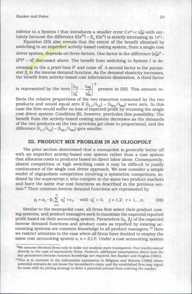
inferior to a System I that introduces a smaller error (I e" I < XM) with cer-tainty because the difference Ein^ - E E(7u*') is strictly increasing In I e° I.

Equation (25) also reveals that the extent of the benefit obtained byswitching to an imperfect activity-based costing system, from a single cost

driver system, depends on three factors. One factor is the difference (x^^ _(e°)2 - ai discussed above. The benefit from switching to System I is de-creasing In the a priori bias e° and noise a?. A second factor is the param-eter pj in the inverse demand function. As the demand elasticity increases,the benefit from activity-based cost information diminishes. A third factor

is represented by the term2

present in (25). This amount re-

fleets the relative proportions of the two resources consumed by the twoproducts and would equal zero if [\J\j^ - (^1/^^,2) were zero. In thiscase the firm would suffer no loss of expected profit by retaining the singlecost driver system. Condition (6). however, precludes this possibility. Thebenefit from the activity-based costing system decreases as the demandsof the two products on the two activities get close to proportional, and thedifference \\X^\Q\ - (^1/^2* S*® smaller.

in . PRODUCT MIX PROBLEM IN AN OLIGOPOLYThe prior section determined that a monopolist is generally better off

with an imperfect activity-based cost system rather than a cost systemthat allocates costs to products based on direct labor alone. Consequently,absent competition or high switching costs It may be difficult to justifycontinuance of the single cost driver approach. We now consider a simplemodel of oligopolistic competition involving n symmetric competitors, in-dexed by the superscript r. who compete in the same two product marketsand have the same true cost functions as described In the previous sec-tion.^ Their common inverse demand functions are represented by

wi thq ;>0 . J = 1.2: r=l , . . .n . (26)r=]

Similar to the monopolist case, all firms first select their product cost-Ing systems, and product managers seek to maximize the expected reportedprofit based on their accounting system. Parameters (a,, p.) of the expectedinverse demand functions and product costs as reported by existing ac-counting systems are common knowledge to all product managers. ° Herewe restrict attention to the case when aU firms have decided to employ thesame cost accounting system s. s = Z.I.P. Under a cost accounting system

^ e assume identical firms only to make our analysis more transparent. Our results extenddirectly to the case of asymmetric firms. However, additional assumptions about how thekey parameters become common knowledge are required. See Banker and Hughes [1991].

'^Thls Is in contrast to the information asymmetry in MUgnim and Roberts 11982] wherepotential entrants do not know the Incumbent's costs, and the established firm may signalits costs with its pricing strategy to deter a potential entrant from entering the market.

24 • Journal of Management Accounting Research, Fall 1993

that estimates the unit variable overhead costs to be hj. the expected re-ported profit of a firm r is given by:

E(n-)=X laj-ftX qj ' -Vj-h jV-f . r=l....n. (27)j=i p=i

First order conditions for the maximization of E(7i:") yield the followingCoumot-Nash equilibrium characterization of optimal quantities under asystem s:

qf = E! ^ . r = l....n. (28)2ft

Consistent conjectures equilibrium (CCE) is an alternative notion of equi-librium in oligopoly models, see e.g., Bresnahan (19811. In our model oflinear cost and Inverse demand functions, the unique CCE Is given by theBertrand-Nash equilibrium, which implies that the prices are set equal tothe (identical) marginal costs of the two firms. In the presence of (longterm) fixed costs, however, the firms cannot survive under such a pricingregime. We have chosen, therefore, to employ the Coumot-Nash criterionto characterize the oligopoly equilibrium concept. Based on the assumedequilibrium concept, the optimal quantity for each firm r under a productcosting system s, is obtained by solving the n equations in (27):''

qf = (aj-vj-hj')/(n+ 1)13,, r= l..,,n. (29)

In this setting, the prices p ' are:

2^ j j ; (30)n + 1 n + 1

Each firm's true expected profit under the optimal quantity choice in(29) is given by:

2

E(7c"-) =X laj - nI3i qf - Vj - hjl qf - f (31)

Comparing the optimal expected profit under a system s with that underSystem P reveals the following difference:

2

'P - S - Vj - hj)(qf - qf) -nft (qf - qf f f

_l( l)(a - Vj - hj) -

(n+

"In the present case, this expression follows immediately from (27) by appealing to thesymmetry resulting from identical firms.

Banker and Potter 25

It follows from (8) that the actual overhead costs x° In the base period

£ire equal to ^ hjq]1=1 I=L.M J=l

. By construction, the esti-

2

mated overhead costs hJ are also such that Y hjq[^ equals x°. This Is

verified easily by referring to the definition of hj. s=Z.I. In (11) and (16).Therefore, we have:

= 0.

We introduce next a concept of inter-perlod consistency of the cost ac-counting system to further simpliiy the expression In (32). In a steady statewhere the parameters . 9,. of the cost and demand functions donot change, the quantities produced of the two products also should re-

main unchanged.'2 That is, in a steady state, the quantity q|^ in the base

period is equal to the quantity qj* in the current period:

and therefore, we have

= qf = (ttj - Vj - h;)/(n +

(hj-hj)qf = 0.

(34)

That is, estimates of total overhead costs based on the (possibly distorted)

product cost estimates (hJ) from a system s are. in fact, unbiased esti-mates of the true total overhead costs in steady state.

We refer to the above conditions in (34) and (35) as the Axiom of Consis-tency in Steady State (ACSS).' Under ACSS. therefore, the second term in(32) vanishes^** and the expression reduces to

(36)2

= X (h; - hj) /(n - 1) PJ > 0j=i

and further, proceeding as in the monopoly case, we have

2(n + 1) ft

' It can be shown that the time series of optimal quantities converges exponentially If thedemand and cost functions do not ehange. Our simulation studies also indicate rapideonvergence (In two to three periods) to steady state following a perturbation in expectedInverse demand or true cost parameters.

' An anonymous referee noted that steady state for cost functions is the same as the commonstandard costing conditions where variances are charged directly against income.

I was not required in the previous section as n - 1 = 0 for a monopoly.

26 Journal of Man(^ement Accounting ResearcK Fall 1993

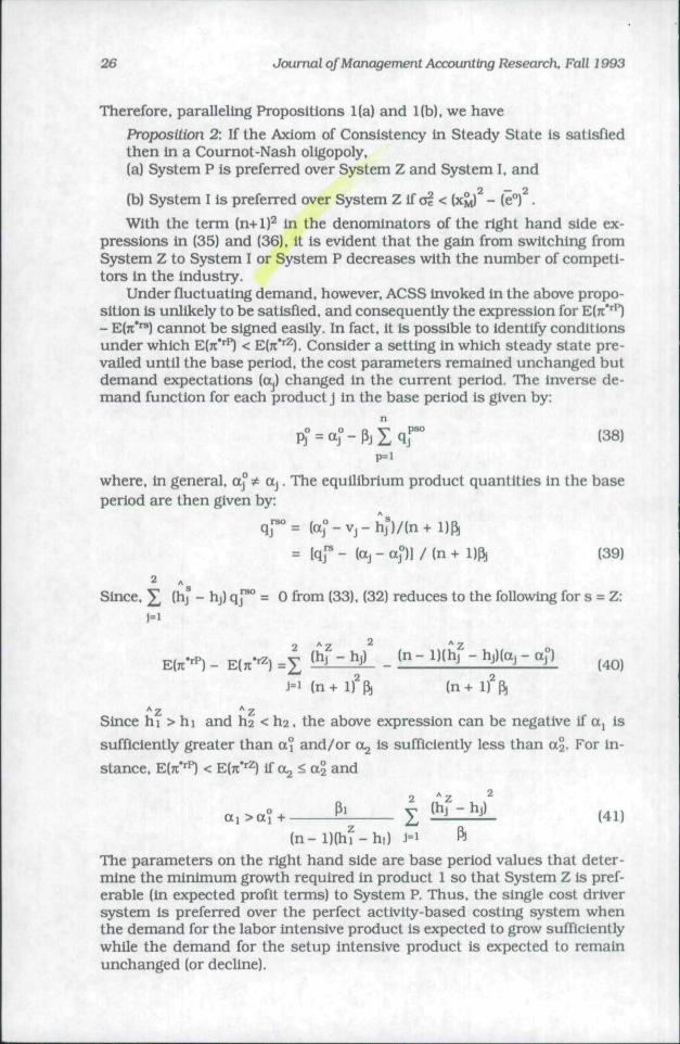
Therefore, paralleling Propositions Ka) and l(b). we have

Proposition 2: If the Axiom of Consistency in Steady State is satisfiedthen In a Cournot-Nash oligopoly,(a) System P Is preferred over System Z and System I, and

(b) System I is preferred over System Z if (^ < (x^ - (e°) .

With the term (n+l)^ in the denominators of the right hand side ex-pressions in (35) and (36), it is evident that the gain from switching fromSystem Z to System I or System P decreases with the number of competi-tors in the industry.

Under fluctuating demand, however. ACSS invoked in the above propo-sition is unlikely to be satisfied, and consequently the expression for E(7i''"n- Edt** ) cannot be signed easily. In fact, it is possible to identify conditionsunder which E(7r'''n < E(7t'' ). Consider a setting in which steady state pre-vailed until the base period, the cost parameters remained unchanged butdemand expectations (a,) changed in the current period. The inverse de-mand function for each product j in the base period is given by:

where, in general, a"^ aj. The equilibrium product quantities in the baseperiod are then given by:

= Iqf- (a j -a;)] / (n-f l)ft (39)

Since, X (hj* - hj) qf" = 0 from (33). (32) reduces to the following for s = Z:1=1

Since hi > hi and h2 < h2. the above expression can be negative if a, Is

sufficiently greater than a° and/or cc is sufficiently less than a2. For in-

stance. EITC"' ' < E(7c" ^ if O; < a2 and

(41)

The parameters on the right hand side are base period values that deter-mine the minimum growth required in product 1 so that System Z is pref-erable (in expected profit terms) to System P. Thus, the single cost driversystem is preferred over the perfect activity-based costing system whenthe demand for the labor intensive product is expected to grow sufilcientlywhile the demand for the setup intensive product is expected to remainunchanged (or decline).

Banker and Potter 27

Dividing the right hand side expression in (41) above by a°. we obtainthe required growth rate in product 1.

61= 1^ ^^ I 2i^-iiiL (42)

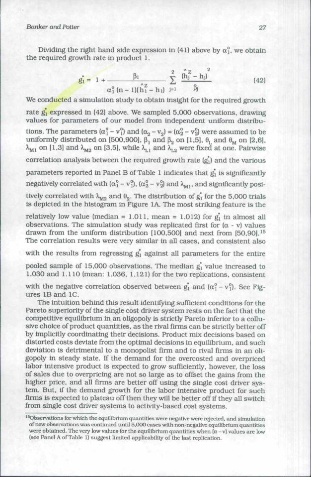
We conducted a simulation study to obtain insight for the required growth

rate g'l expressed in (42) above. We sampled 5.000 observations, drawingvalues for parameters of our model from independent uniform distribu-tions. The parameters (a? - v°) and {a^ - V2) = (a^ - v?) were assumed to beuniformly distributed on (500.9001. Pi and pj on [1.5], 6 and 9^ on [2.61.X i on (1.31 and X^^ °^ 13.51. while ^ , and > 2 ^ ^ fixed at one. Pairwise

correlation analysis between the required growth rate (g]) and the variousparameters reported in Panel B of Table 1 indicates that g, is significantlynegativelycorrelated with (a°-v°).(a2-v5) and Xj p and significantly posi-tively correlated with Xj^^ ^"^ ^2- ' ^ ^ distribution of g] for the 5.000 trialsis depicted in the histogram in Figure lA. The most striking feature is the

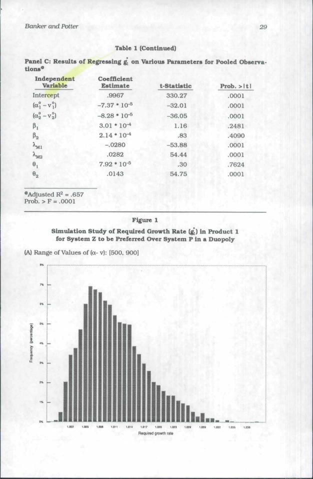
relatively low value (median = 1.011. mean = 1.012) for g, in almost allobservations. The simulation study was replicated first for (a - v) valuesdrawn from the uniform distribution (1OO.5CX)1 and next from [50.901.'^The correlation results were very similar in all cases, and consistent also

with the results from regressing gi against all parameters for the entire

pooled sample of 15.000 observations. The median g'l value increased to1.030 and 1.110 (mean: 1.036. 1.121) for the two replications, consistent

with the negative correlation observed between gj and (a? - v°). See Fig-ures IB and lC.

The intuition behind this result identifying sufficient conditions for thePareto superiority of the single cost driver system rests on the fact that thecompetitive equilibrium in an oligopoly is strictly Pareto inferior to a collu-sive choice of product quantities, as the rival firms can be strictly better offby implicitly coordinating their decisions. Product mix decisions based ondistorted costs deviate from the optimal decisions in equilibrium, and suchdeviation is detrimental to a monopolist firm and to rival firms in an oli-gopoly in steady state. If the demand for the overcosted and overpricedlabor intensive product is expected to grow sufficiently, however, the lossof sales due to overpricing are not so large as to offset the gains from thehigher price, and all firms are better off using the single cost driver sys-tem. But. if the demand growth for the labor intensive product for suchflrms is expected to plateau off then they will be better off if they all switchfrom single cost driver systems to activity-based cost systems.

^Observations for which the equilibrium quantities were negative were rejected, and simulationof new observations was continued until 5,000 cases with non-negative equilibrium quantitieswere obtained. The very low values for the equilibrium quantities when (a - v) values are low(see Panel A of Table 1) suggest limited applicabiliiy of the last replication.

28 Joumal of Management Accounting ResearcK Fall 1993

Table 1

Simulation Study to Examine Required Growth Rate g,

Panel A: Descriptive Statistics

& • •

qf:

qf:

qf:

qf:

MeanStd. Dev91Median93

MeanStd. Dev

MeanStd. Dev

MeanStd. Dev

MeanStd. Dev

Range of Values for (a*- T°) and (a^- V2)[500. 900]

1.012.0071.0071.0111.016

91.67047.863

89.78846.374

91.18647.779

90.27046.448

[100. BOO]

1.036.0251.0191.0301.047

39.57026.308

36.90724.816

39.08326.302

37.40024.810

[50. 90|

1.121.0671.0721.1101.159

8.2064.410

6.0673.515

7.7224.330

6.5473.545

Panel B: Pearson Correlation of gj with Various Parameters'

Range of Values for (a ' - v*) and (a*- v*)

P.

[5OO. 9OO]

-.1706(.0001)

-.1791(.0001)

-.0243(.0854)

.0192(.1748)

-.5462(.0001)

.5393(.0001)

-.0233(.0995)

.5452(.0001)

[100. 500]

-.2858(.0001)

-.3731(.0001)

.0121(.3911)

.0209(.1387)

-.4229(.0001)

.4196(.0001)

.0065(.6485)

.4228(.0001)

[50. 90]

-.1005(.0001)

-.2359(.0001)

.0142(.3147)

.0083(.3466)

-.5429(.0001)

.5276(.0001)

-.0058(.6816)

.5466(.0001)

•significance levels are ln parentheses

Banker and Potter 29

Table 1 (Continued)

Panel C: Results of Regressing g* on Various Parameters for Pooled Obserra-tions^

IndependentVariable

Intercept, O Oi

(cti-v,)(a^-v^)

P.P2

^ 1

^ 2

e,^ 2

•Adjusted R = .657Prob. > F = .0001

CoefficientEstimate

.9967-7.37 • 10-^

-8.28 * l a *3.01 • 10-*2.14* 10-^

-.0280.0282

7.92 • 10-*.0143

t Statistic330.27-32.01

-36.051.16.83

-53.8854.44

.30

54.75

Prob. >ltl.0001.0001

.0001

.2481

.4090

.0001

.0001

.7624

.0001

Figure 1

Simulation Study of Required Growth Rate (g*) in Product 1for System Z to be Preferred Over System P In a Duopoly

(A) Range of Values of (a- v): (500. 900]

I I.UI 1.0I&

Required giowrth rai»

30 Jourrwd of Management Accounting Research, Fall 1993

Figure 1 (Continued)

(B) Range of Values of (a - v): [100. 500]

I l l l lRequtrod gtmvth raM

(C) Range of Values of (a - v): [50. 90)

I l l l l III1.W i.M 1.11 vi> LM vn ' H

Required gmwth rate

Banker and Potter

IV. CONCLUDING REMARKSMany claims about the value of an activity-based costing system have

been made by Us advocates and opponents. These claims, however, havenot been subjected to the scrutiny of a rigorous model that reflects rationalbehavior by users of product costing systems. We take a step in this direc-tion by analytically examining how the inclusion of multiple cost driversalters the value of a product costing system. Our analysis evaluates theimpact a single cost driver and a multiple cost driver system have on theoptimal expected profits of a monopolist, and alternatively firms compet-ing in an oligopoly. We find that generally a monopolist firm can expecthigher profit if It selects its product mix using a multiple cost driver sys-tem even when the system is Imperfect in assigning overhead costs to thevarious activities. In particular, the value of an imperfect ABC system de-creases with Its noisiness. In an oligopoly setting, a similar result obtainsif the cost and demand parameters do not change.

While these results ordering the value of the cost systems are intu-itively appealing because they parallel those based on the coarseness ofinformation partitions, such simple interpretations do not extend to thegeneral competitive setting. In particular, we show that the equilibriumImplemented by the rival firms using a direct labor-based cost accountingsystem is Pareto superior to that implemented under an accurate activity-based cost accounting system when the demand for the overcosted laborintensive product is expected to grow sufficiently relative to the demandfor the undercosted setup intensive product. In other words, facing imper-fect competition, it is sometimes optimal for firms to persist in using asingle cost driver system rather than switching to an activity-based costsystem. Our analysis also indicates that the benefits from an ABC systemwill likely be more pronounced in industries ln which the demand growthfor traditional direct labor-Intensive products is small relative to that forproducts intensive in other cost drivers.

32 Journal of Management Accounting ResearcK Fall 1993

REFERENCESAlles, M., "A Model of Strategic Costing." Stanford University, working paper (1991).Banker. R D., and J. S. Hughes, "Product Costing and Pricing." University of Minnesota,

working paper (1991)., and H. H. Johnston, "An Empirical Study of Cost Drivers in the U.S. Airline Industry,"

The Acxxiunting Review [July 1993), pp. 576-6O1., G. Potter, and R Schroeder, "Empirical Analysis of Manufacturing Overhead Costs in

U.S. Plants." Unlversiiy of Minnesota, working paper (1992).-. and . "Strategic Choice of Produet Costing Systems." University of Minnesota,

working paper (1992).Bresnahan, T. F., "Duopoly Models with Consistent Conjectures." American Economic Review

(December 1981), pp. 934-945.Cooper, R, "Does Your Company Need a New Cost System?" Journal ojCost Management

(Spring 1987), pp. 45-49.. and R S. Kaplan, "How Cost Accounting Systematically Distorts Product Costa." Chapter

9 In W. Bruns and R Kaplan (Eds.), Accounting & Management Field Study Perspectives(Harvard Business School Press, 1987). pp. 204-228.

Fershtman. C, and K. Judd," E^quilibrium Incentives in Oligopoly." American Economic Re-view (December 1987), pp. 927-940.

Foster, G., and M. Gupta, "Manufacturing Overhead Cost Driver Analysis," Journal of Ac-counting and Ekxfnomics (January 1990). pp. 309-337.

Johnson. H. T., and R S. Kaplan, Relevance Lost, Harvard Business School Press, 1987.Mllgrom, P.. and J. Roberis. "Limit Pricing and Entiy Under Incomplete Infonnation: An Equi-

librium Analysis," Econometrica (March 1982), pp. 443-460.Miller, J. G., and J. Kim, "Beyond the Quality Revolution: U.S. Manufacturing Strategy in the

1990s" (Boston UniversUy. 1990).. and T. E. VoUmann, "The Hidden Factory," Harvard Business Review (September-

October 1985), pp. 142-150.Schiff, J. B., (Ed.), Cost Management Update, National Association of Accountants (January

1991), pp. 1-2.Shank. J. K.. and V. Govindarajan, "The Perils of Cost Allocation Based on Production Vol-

umes." Accounting Horizons (December 1988), pp. 71-79.