on the cost implications of technical energy losses on

International Journal of Science and Research (IJSR) ISSN (Online): 2319-7064

Index Copernicus Value (2013): 6.14 | Impact Factor (2014): 5.611

Volume 5 Issue 1, January 2016

www.ijsr.net Licensed Under Creative Commons Attribution CC BY

On The Cost Implications of Technical Energy

Losses on Nigerian 330-kV Transmission Grid

System

Ademola Abdulkareem1, Awosope Claudius

2, Ayokunle Awelewa

3

1,2,3 Electrical and Information Engineering Department, College of Engineering, Covenant University, Ota, Nigeria

Abstract: Base on the author’s result of power line losses obtained for low, medium and high current levels as 146.73MW, 322.24MW

and 738.28MW respectively, in his bid to evaluate the power line losses using symmetrical component theory of unbalanced fault, the

annual energy (MWH) losses for year 2013 was calculated and validated in this study. The annual technical energy losses due to the low,

medium and high power losses were respectively found to be 443.45GWH, 976.895GWH and 2231.230GWHbased on Load Factor and

Load Loss Factor amounting to N8.4 billion, N18.6 billion and N42.4 billion respectively. The low power loss (steady-state) result of this

work was validated by the result of load-flow obtained using the MATLAB and Power Word Simulator (PWS) while the annual MWH

for the high power loss level compares favourably well with the normal practice of utility operator’s monthly energy balance thereby

closing the gap between the practical information and the theoretical one.

Keywords: Power line losses, Current levels, Load Factor, Load Loss Factor, Load-Flow

1. Introduction

Power quality has become an important issue for

maximum efficiency operation of energy that is delivered

to transmission and distribution line. The more the power

that flows through the network, the more the current and

hence the voltage drop becomes more excessive and power

quality declines. The global problem of the lower power

availability to consumers is a consequence of power loss

and no matter how carefully the power system network is

designed, losses are inevitable. Loss of power on

transmission lines is a global problem and it is necessary

to state here that the losses on transmission lines can result

into line outages in the electric power system. The existing

transmission system in Nigeria is characterized by high

line losses and several outages leading to interruption of

systems and equipment. Nigerian electricity grid has a

large proportion of transmission and distribution losses,

and these amounts to a whopping 44.5% of generation [1].

Based on the Power Holding Company of Nigeria (PHCN)

annual reports for the 2004 and 2005, the transmission line

losses alone were estimated to be 9.2% [2]. Countries such

as China that have attached importance to loss

minimization to enhance efficiency have about 13%

transmission and distribution losses with India having

about 23% [3]. The losses in some other countries like

Iraq, Moldova, Sudan, Venezuelan RB, Syria, Korea

Republic, Yemen Republic, Pakistan, Tanzania, México,

Taiwan, U.S.A, and Japan are 42, 40, 28, 27, 26, 25, 22,

20, 16, 9, 6 and 5% respectively [4].

However, going by the available data and tools needed for

calculating technical losses in power system, current

techniques have certain drawbacks regarding such

calculations.Moreover, literature reveals different methods

of loss estimation but the existing approaches focus mainly

on theoretical calculation and probabilistic data that are

based on simple model data, insufficient to give a correct

evaluation assessment of losses [5]. Hence, there is still a

clear gap between practical information and the theoretical

one which tends to be poor and not precise [6] and the

reduction of system losses is analyzed on the accuracy of

the technical losses. To solve the challenging problems

inherent in designing future power systems to deliver

increasing amounts of electrical energy in a safe, clean and

economical manner [7], a regular and fairly accurate

description of power losses as a function of time to make a

reliable prediction of energy losses is required. The

objective of this study, therefore, is to evaluate the

technical losses in and its cost implication on Nigeria 330-

kV power transmission system.

2. Methodology

The methodology adopted for this study is the analysis of

the disturbances brought about by the faults followed by

the procedure for maximum line currents determination

that is used to calculate the power losses and the values are

used thereafter to evaluate the annual energy losses and its

cost implications in the Nigeria 330-kV power

transmission system. Results analysis of load-flows using

the code-based MATLAB and Power World Simulation

model-based software are presented and discussed.

2.1 Disturbances in Nigeria 330-kV Transmission

System

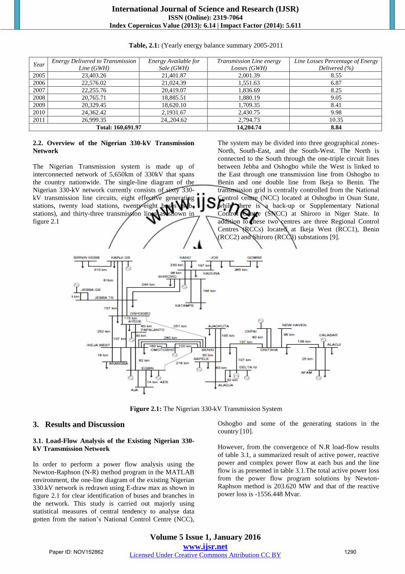
Table 2.1 gives the summary of the yearly energy balance

that reflects a total loss of 14204.74GWH from 2005 to

2011 as reported in the PHCN monthly energy balance

summary.. These transmission losses - calculated to be

approximately 10.05% of the energy fed into the grid [8],

clearly show that majority of the outages in NESI are

responsible for the problem in the transmission network.

Paper ID: NOV152862 1289





Table, 2.1: (Yearly energy balance summary 2005-2011

Year Energy Delivered to Transmission

Line (GWH)

Energy Available for

Sale (GWH)

Transmission Line energy

Losses (GWH)

Line Losses Percentage of Energy

Delivered (%)

2005 23,403.26 21,401.87 2,001.39 8.55

2006 22,576.02 21,024.39 1,551.63 6.87

2007 22,255.76 20,419.07 1,836.69 8.25

2008 20,765.71 18,885.51 1,880.19 9.05

2009 20,329.45 18,620.10 1,709.35 8.41

2010 24,362.42 2,1931.67 2,430.75 9.98

2011 26,999.35 24,,204.62 2,794.73 10.35

Total: 160,691.97 14,204.74 8.84

2.2. Overview of the Nigerian 330-kV Transmission

Network

The Nigerian Transmission system is made up of

interconnected network of 5,650km of 330kV that spans

the country nationwide. The single-line diagram of the

Nigerian 330-kV network currently consists of sixty 330-

kV transmission line circuits, eight effective generating

stations, twenty load stations, twenty-eight buses (sub-

stations), and thirty-three transmission lines as shown in

figure 2.1

The system may be divided into three geographical zones-

North, South-East, and the South-West. The North is

connected to the South through the one-triple circuit lines

between Jebba and Oshogbo while the West is linked to

the East through one transmission line from Oshogbo to

Benin and one double line from Ikeja to Benin. The

transmission grid is centrally controlled from the National

Control centre (NCC) located at Oshogbo in Osun State,

while there is a back-up or Supplementary National

Control Centre (SNCC) at Shiroro in Niger State. In

addition to these two centres are three Regional Control

Centres (RCCs) located at Ikeja West (RCC1), Benin

(RCC2) and Shiroro (RCC3) substations [9].

Figure 2.1: The Nigerian 330-kV Transmission System

3. Results and Discussion

3.1. Load-Flow Analysis of the Existing Nigerian 330-

kV Transmission Network

In order to perform a power flow analysis using the

Newton-Raphson (N-R) method program in the MATLAB

environment, the one-line diagram of the existing Nigerian

330.kV network is redrawn using E-draw max as shown in

figure 2.1 for clear identification of buses and branches in

the network. This study is carried out majorly using

statistical measures of central tendency to analyse data

gotten from the nation’s National Control Centre (NCC),

Oshogbo and some of the generating stations in the

country [10].

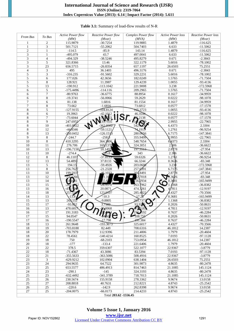
However, from the convergence of N.R load-flow results

of table 3.1, a summarized result of active power, reactive

power and complex power flow at each bus and the line

flow is as presented in table 3.1.The total active power loss

from the power flow program solutions by Newton-

Raphson method is 203.620 MW and that of the reactive

power loss is -1556.448 Mvar.






Table 3.1: Summary of load-flow results of N-R

From Bus To Bus Active Power flow

(MW)

Reactive Power flow

(Mvar)

Complex Power flow

(MVA)

Active Power loss

(MW)

Reactive Power loss

(Mvar)

1 2 115.9879 -30.7254 119.9885 1.4879 -116.625

1 3 501.7121 -55.2062 504.7403 6.633 -11.5062

2 1 -114.5 -85.9 143.14 1.4879 -116.625

3 1 -495.079 43.7 497.0041 6.633 -11.5062

3 4 -494.329 -38.5246 495.8279 0.671 -2.3843

3 5 321.8366 13.46 322.1179 5.6016 -78.1002

3 23 656.5715 -26.8354 657.1197 26.6503 75.2551

4 3 495 36.1403 496.3176 0.671 -2.3843

5 3 -316.235 -91.5602 329.2231 5.6016 -78.1002

5 6 177.026 42.3656 182.0249 1.5765 -71.7504

5 8 128.921 11.3987 129.4239 1.0055 -93.4136

5 13 -190.912 -113.1042 221.9008 3.238 -172.5968

6 5 -175.4496 -114.116 209.2965 1.5765 -71.7504

6 7 -80.9763 -36.6775 88.8954 0.1617 -34.9959

6 8 -19.3741 -56.0066 59.2629 0.0222 -98.1078

7 6 81.138 1.6816 81.1554 0.1617 -34.9959

7 8 73.662 -1.6816 73.6812 0.0577 -17.1578

8 5 -127.9155 -104.8124 165.3723 1.0055 -93.4136

8 6 19.3963 -42.1012 46.3544 0.0222 -98.1078

8 7 -73.6044 -15.4763 75.2138 0.0577 -17.1578

8 9 247.6955 235.7035 341.9199 2.9955 -22.7965

8 10 -403.8922 -362.0502 542.4106 6.4373 2.3304

8 12 -44.8346 -59.1121 74.1915 1.2761 -96.9254

8 13 -250.0452 -126.1513 280.0656 6.7175 -147.3841

9 8 -244.7 -258.5 355.9499 2.9955 -22.7965

10 8 410.3295 364.3806 548.7654 6.4373 2.3304

10 11 276.706 169.1378 324.3051 2.306 -36.6622

10 13 -196.7158 18.1493 197.5513 2.8778 -27.954

11 10 -274.4 -205.8 343 2.306 -36.6622

12 8 46.1107 -37.8133 59.6326 1.2761 -96.9254

12 13 54.4893 37.8133 66.3244 0.3626 -83.348

13 5 194.15 -59.4926 203.0606 3.238 -172.5968

13 8 256.7627 -21.2328 257.6391 6.7175 -147.3841

13 10 199.5937 -46.1033 204.8491 2.8778 -27.954

13 12 -54.1266 -121.1613 132.7018 0.3626 -83.348

13 14 14.1681 -155.6499 156.2934 0.3681 -165.9499

13 15 -262.4152 -26.9578 263.7962 1.1368 -36.8382

13 16 -473.9006 20.0871 474.3261 4.7811 -12.9197

13 18 -257.5321 123.0107 285.4022 4.4327 -70.3566

14 13 -13.8 -10.3 17.22 0.3681 -165.9499

15 13 263.552 -9.8805 263.7372 1.1368 -36.8382

15 17 -93.852 3.7389 93.9265 0.2026 -50.8631

16 13 478.6817 -33.0068 479.8183 4.7811 -12.9197

16 17 191.3183 -28.4304 193.4192 0.7637 -46.2284

17 15 94.0547 -54.602 108.755 0.2026 -50.8631

17 16 -190.5547 -17.798 191.384 0.7637 -46.2284

18 13 261.9648 -193.3673 325.6017 4.4327 -70.3566

18 19 -703.8188 82.449 708.6316 46.1812 14.2387

18 20 178.7979 112.9396 211.4806 1.7979 -20.4604

18 22 78.4561 -140.4214 160.8525 7.0193 -97.1128

19 18 750 -68.2103 753.0954 46.1812 14.2387

20 18 -177 -133.4 221.6406 1.7979 -20.4604

21 22 378.5 359.6307 522.1077 22.9367 -3.8779

22 18 -71.4367 43.3086 83.5394 7.0193 -97.1128

22 21 -355.5633 -363.5086 508.4916 22.9367 -3.8779

23 3 -629.9212 102.0904 638.1404 26.6503 75.2551

23 24 294.9635 64.7522 301.9873 4.8635 -80.2478

23 25 653.5577 486.4913 814.7463 21.1085 145.1124

24 23 -290.1 -145 324.3193 4.8635 -80.2478

25 23 -632.4492 -341.3789 718.7013 21.1085 145.1124

25 26 230.5674 155.9158 278.3362 9.9674 13.0158

25 27 208.8818 40.7631 212.8221 4.8743 -25.2542

26 25 -220.6 -142.9 262.8398 9.9674 13.0158

27 25 -204.0075 -66.0173 214.4233 4.8743 -25.2542

Total 203.62 -1556.45






Another load-flow analysis was carried out on the same

330-kV transmission network (for the purpose of

comparison) using the run mode of power world simulator

[11]. The line flows and power losses are as presented in

table 3.2. The load-flow is performed at a steady state and

therefore these results are obtained under normal

condition. The load-flow analysis was performed at a

steady state; the power-flow solution results obtained for

PWS and MATLAB software are compared with the

results of low power obtained from LC that is likened to

the current that flows under a steady-state condition for

validation.

Figure 3.1: The Simulation run Mode of Existing Nigerian 330-kV Transmission Network

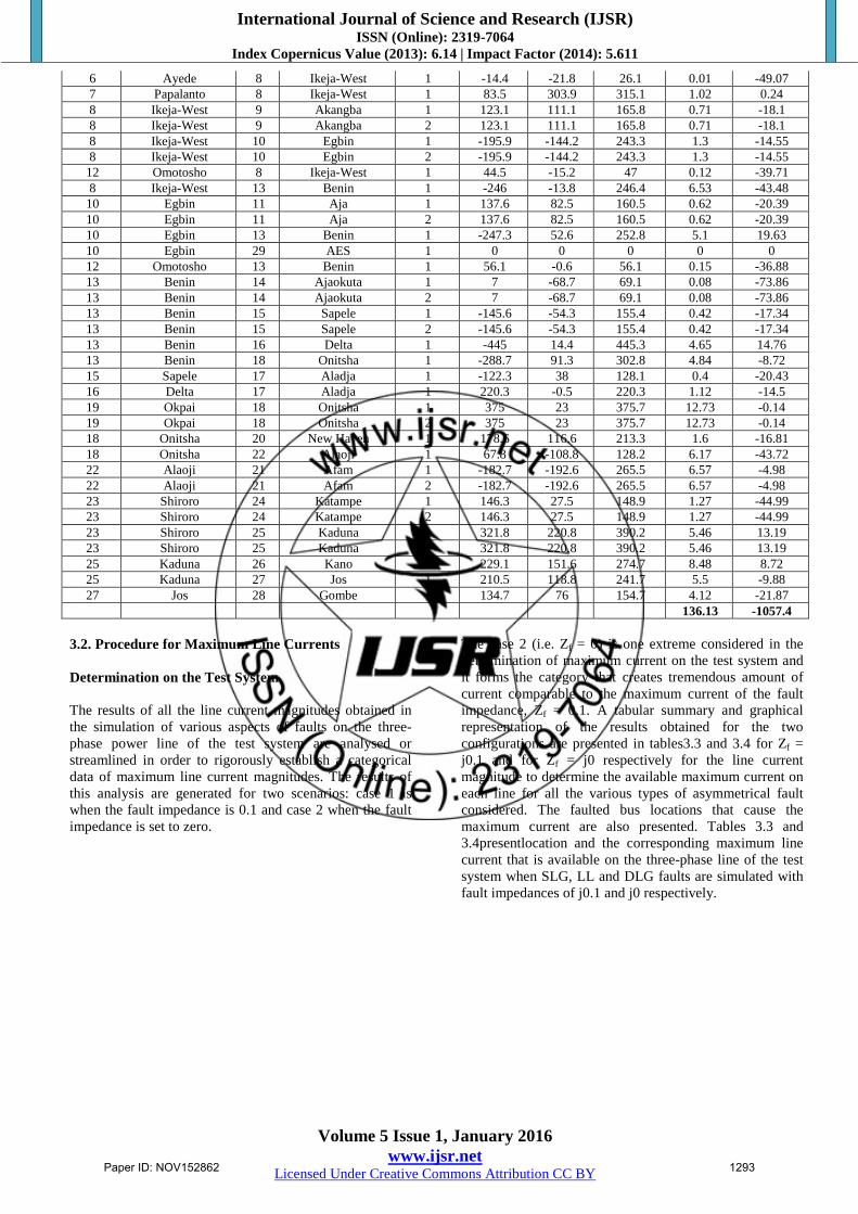
Table 3.2: Line-Flows and Power losses for PWS Model-Based Network

From

Bus No From Name

To

Bus

No

To Name Circuit MW From Mvar

From

MVA

From MW Loss Mvar Loss

1 Kainji 2 Birnin-Kebbi 1 116.7 48.5 126.4 2.2 -37.42

1 Kainji 3 Jebba TS 1 250.5 -36.7 253.2 1.83 -15.25

1 Kainji 3 Jebba TS 2 250.5 -36.7 253.2 1.83 -15.25

3 Jebba TS 4 Jebba GS 1 -247.3 31.8 249.4 0.19 -2.07

3 Jebba TS 4 Jebba GS 2 -247.3 31.8 249.4 0.19 -2.07

3 Jebba TS 5 Oshogbo 1 116.7 -10.7 117.2 0.78 -52.18

3 Jebba TS 5 Oshogbo 2 116.7 -10.7 117.2 0.78 -52.18

3 Jebba TS 5 Oshogbo 3 116.7 -10.7 117.2 0.78 -52.18

3 Jebba TS 23 Shiroro 1 315.5 -41.3 318.1 6.67 -22.81

3 Jebba TS 23 Shiroro 2 315.5 -41.3 318.1 6.67 -22.81

5 Oshogbo 6 Ayede 1 192.3 3.5 192.3 1.59 -28.35

5 Oshogbo 8 Ikeja-West 1 130 -9.9 130.4 1 -48.67

5 Oshogbo 13 Benin 1 -175.8 -20 176.9 2.89 -68.38

6 Ayede 7 Papalanto 1 -70.7 -153.2 168.7 0.6 -13.71






6 Ayede 8 Ikeja-West 1 -14.4 -21.8 26.1 0.01 -49.07

7 Papalanto 8 Ikeja-West 1 83.5 303.9 315.1 1.02 0.24

8 Ikeja-West 9 Akangba 1 123.1 111.1 165.8 0.71 -18.1

8 Ikeja-West 9 Akangba 2 123.1 111.1 165.8 0.71 -18.1

8 Ikeja-West 10 Egbin 1 -195.9 -144.2 243.3 1.3 -14.55

8 Ikeja-West 10 Egbin 2 -195.9 -144.2 243.3 1.3 -14.55

12 Omotosho 8 Ikeja-West 1 44.5 -15.2 47 0.12 -39.71

8 Ikeja-West 13 Benin 1 -246 -13.8 246.4 6.53 -43.48

10 Egbin 11 Aja 1 137.6 82.5 160.5 0.62 -20.39

10 Egbin 11 Aja 2 137.6 82.5 160.5 0.62 -20.39

10 Egbin 13 Benin 1 -247.3 52.6 252.8 5.1 19.63

10 Egbin 29 AES 1 0 0 0 0 0

12 Omotosho 13 Benin 1 56.1 -0.6 56.1 0.15 -36.88

13 Benin 14 Ajaokuta 1 7 -68.7 69.1 0.08 -73.86

13 Benin 14 Ajaokuta 2 7 -68.7 69.1 0.08 -73.86

13 Benin 15 Sapele 1 -145.6 -54.3 155.4 0.42 -17.34

13 Benin 15 Sapele 2 -145.6 -54.3 155.4 0.42 -17.34

13 Benin 16 Delta 1 -445 14.4 445.3 4.65 14.76

13 Benin 18 Onitsha 1 -288.7 91.3 302.8 4.84 -8.72

15 Sapele 17 Aladja 1 -122.3 38 128.1 0.4 -20.43

16 Delta 17 Aladja 1 220.3 -0.5 220.3 1.12 -14.5

19 Okpai 18 Onitsha 1 375 23 375.7 12.73 -0.14

19 Okpai 18 Onitsha 2 375 23 375.7 12.73 -0.14

18 Onitsha 20 New Haven 1 178.6 116.6 213.3 1.6 -16.81

18 Onitsha 22 Alaoji 1 67.8 -108.8 128.2 6.17 -43.72

22 Alaoji 21 Afam 1 -182.7 -192.6 265.5 6.57 -4.98

22 Alaoji 21 Afam 2 -182.7 -192.6 265.5 6.57 -4.98

23 Shiroro 24 Katampe 1 146.3 27.5 148.9 1.27 -44.99

23 Shiroro 24 Katampe 2 146.3 27.5 148.9 1.27 -44.99

23 Shiroro 25 Kaduna 1 321.8 220.8 390.2 5.46 13.19

23 Shiroro 25 Kaduna 2 321.8 220.8 390.2 5.46 13.19

25 Kaduna 26 Kano 1 229.1 151.6 274.7 8.48 8.72

25 Kaduna 27 Jos 1 210.5 118.8 241.7 5.5 -9.88

27 Jos 28 Gombe 1 134.7 76 154.7 4.12 -21.87

136.13 -1057.4

3.2. Procedure for Maximum Line Currents

Determination on the Test System

The results of all the line current magnitudes obtained in

the simulation of various aspects of faults on the three-

phase power line of the test system are analysed or

streamlined in order to rigorously establish a categorical

data of maximum line current magnitudes. The results of

this analysis are generated for two scenarios: case 1 is

when the fault impedance is 0.1 and case 2 when the fault

impedance is set to zero.

The case 2 (i.e. Zf = 0) is one extreme considered in the

determination of maximum current on the test system and

it forms the category that creates tremendous amount of

current comparable to the maximum current of the fault

impedance, Zf = 0.1. A tabular summary and graphical

representation of the results obtained for the two

configurations are presented in tables3.3 and 3.4 for Zf =

j0.1 and for Zf = j0 respectively for the line current

magnitude to determine the available maximum current on

each line for all the various types of asymmetrical fault

considered. The faulted bus locations that cause the

maximum current are also presented. Tables 3.3 and

3.4presentlocation and the corresponding maximum line

current that is available on the three-phase line of the test

system when SLG, LL and DLG faults are simulated with

fault impedances of j0.1 and j0 respectively.






Table 3.3: Maximum line current caused by SLG, LL, DLG and Location when Zf = j0.1

From - To

bus SLG (pu) Location L - L (pu) Location DLG (pu) Location

1-2 4.7596 BirninKebbi 7.1658 BirninKebbi 8.973 BirninKebbi

3-1 8.5218 JebbaTs 3.1828 Kainji 9.3828 Kainji

4-3 16.4165 Oshogbo 3.2043 JebbaTs 5.615 JebbaTs

5-3 10.3361 JebbaTs 3.7182 Kainji 3.7935 JebbaTs

6-5 11.4695 Papalanta 3.5445 Ayede 5.831 Ayede

7-6 7.5392 Akangba 1.4389 Papalanto 3.2273 Ikeja West

8-6 12.0213 Papalanto 3.5589 Ayede 5.6907 Ayede

8-7 7.6034 Papalanto 1.0787 Osogbo 3.6238 Ayede

8-5 23.9129 Ikeja West 6.2204 Papalanto 10.541 Papalanto

8-9 12.4105 Egbin 4.6204 Akangba 7.3992 Akangba

10-8 11.3709 Akangba 3.3964 Ikeja West 5.3705 Ikeja West

10-11 14.2855 Omotosho 4.7743 Aja 7.8635 Aja

12-8 2.1338 Sapele 8.3932 Ajaokuta 8.3932 Benin

12-13 4.3169 Benin 4.4479 Omotosho 4.3787 Ajaokuta

13-10 9.7498 Aja 7.7994 Ajaokuta 7.7994 Benin

13-8 4.2561 Akangba 1.0363 Ikeja West 3.6871 Omotosho

13-5 9.256 Ayede 12.3477 Ajaokuta 12.3477 Benin

13-18 9.8673 Sapele 13.8204 Sapele 22.6256 Sapele

14-13 7.1047 Aja 10.776 Ajaokuta 10.7761 Benin

15-13 2.6304 Ajaokuta 8.2326 Ajaokuta 8.23255 Benin

15-17 5.4213 Aja 3.4523 Sapele 24.0364 Aladja

16-13 4.6151 Aladja 8.6404 Aladja 21.9803 Aladja

16-17 1.5931 Aja 7.9062 Aladja 5.8227 Benin

18-20 7.0294 New Haven 10.6699 New Heaven 15.7524 Okpai

19-18 2.5873 Benin 2.5873 Benin 4.1100 Alaoji

21-22 3.8533 Onitsha 5.7873 Ajaokuta 6.8982 Onitsha

22-18 10.8159 Alaoji 13.9714 Alaoji 25.4175 Alaoji

23-3 4.1506 JebbaTs 2.496 Shiroro 5.2994 Shiroro

23-24 3.5248 Katampe 5.5056 Katampe 7.45595 Katampe

23-25 5.1388 Kaduna 5.1385 Kaduna 9.67325 Kaduna

25-26 4.8543 Kano 6.7731 Kano 7.7021 Kano

25-27 4.386 Jos 6.3477 Jos 7.695 Jos

27-28 2.9706 Gombe 4.022 Gombe 4.552 Gombe

Note: Black = Low current (LC), Blue = Medium current (MC); Yellow = High Current (HC)

Table 3.4: Maximum line current caused by SLG, LL, DLG and Location when Zf = j0

From - To bus SLG (pu) Location L - L (pu) Location DLG (pu) Location

1-2 5.7715 BirninKebbi 8.0049 BirninKebbi 8.521 BirninKebbi

3-1 7.638 Kainji 8.6994 Kainji 9.9115 Kainji

4-3 11.8103 JebbaTs 15.5621 JebbaTs 16.6508 JebbaTs

5-3 6.7635 Osogbo 9.876 Osogbo 10.3859 Osogbo

6-5 8.0217 Ayede 10.7309 Ayede 11.4168 Ayede

7-6 5.0456 Ikeja West 7.2605 Ikeja West 7.5195 Ikeja West



8-5 16.4218 Papalanto 22.3493 Papalanto 23.6863 Papalanto

8-9 8.5826 Akangba 11.5117 Akangba 12.184 Akangba


10-11 9.4079 Aja 13.2802 Aja 13.962 Aja

12-8 6.5397 Omotosho 8.2427 Benin 8.5784 Benin

12-13 7.0578 Benin 5.981 Omotosho 6.5929 Omotosho

13-10 6.4179 Egbin 9.3047 Egbin 9.759 Egbin


13-5 6.2546 Osogbo 8.7459 Osogbo 9.2419 Osogbo


14-13 7.2072 Benin 10.4319 Benin 10.8361 Benin

15-13 5.590 Benin 7.9602 Benin 8.2957 Benin









18-20 10.5221 Okpai 14.2337 Okpai 17.5902 Okpai


21-22 5.362 Onitsha 6.6105 Onitsha 6.83945 Onitsha


23-3 5.7098 JebbaTs 7.9588 JebbaTs 4.19125 JebbaTs

23-24 4.77465 Katampe 6.762 Katampe 7.10515 Katampe

23-25 7.0505 Kaduna 8.9056 Kaduna 9.29395 Kaduna

25-26 5.3429 Kano 7.1218 Kano 7.4349 Kano

25-27 5.1403 Jos 6.893 Jos 7.3189 Jos

27-28 3.2031 Gombe 4.1324 Gombe 4.386 Gombe

Red = Available maximum current (AMC)

3.3. Evaluation of Technical Power Loss on the Power

Line Test System

Here, the calculation of technical power losses is carried

out on the power line test system i.e the Nigerian 330-kV

transmission system, using the results obtained in tables3.3

and based on the established peak line currents for both

average (LC/MC) and maximum (HC/AMC) line current

magnitudes.

Typical Base Values at 100MVA Base for the Nigerian

330-kV System

𝑉𝑏 =𝑉𝐿

3=

330 × 103

3= 190.5255𝑘𝑉

Ι𝑏 =𝑀𝑉𝐴𝑏

3𝑉𝑏=

100 × 106

3 × 190.5255 × 103

= 174.9546𝐴 𝑜𝑟 0.175𝑘𝐴

𝑅𝑏 = 𝑉𝑏

Ι𝑏=

190.5255 ×103

174.9546= 1089Ω

Using the above base values, the pu line current magnitude

and line resistance are converted to their actual values.

Thus, the power losses for LC, MC, HC and AMC are

computed using equation 3.1.

P = I2R……………… (3.1);

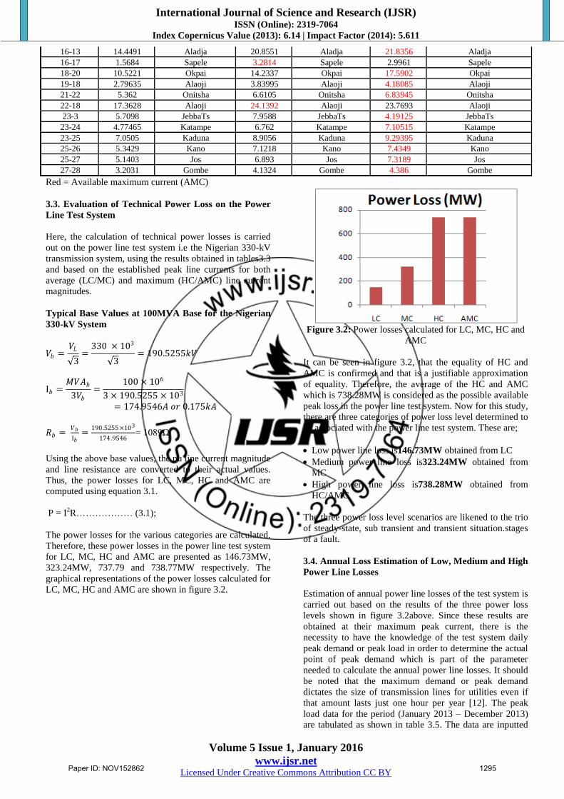
The power losses for the various categories are calculated.

Therefore, these power losses in the power line test system

for LC, MC, HC and AMC are presented as 146.73MW,

323.24MW, 737.79 and 738.77MW respectively. The

graphical representations of the power losses calculated for

LC, MC, HC and AMC are shown in figure 3.2.

Figure 3.2: Power losses calculated for LC, MC, HC and

AMC

It can be seen in figure 3.2, that the equality of HC and

AMC is confirmed and that is a justifiable approximation

of equality. Therefore, the average of the HC and AMC

which is 738.28MW is considered as the possible available

peak loss in the power line test system. Now for this study,

there are three categories of power loss level determined to

be associated with the power line test system. These are;

Low power line loss is146.73MW obtained from LC

Medium power line loss is323.24MW obtained from

MC

High power line loss is738.28MW obtained from

HC/AMC

The three power loss level scenarios are likened to the trio

of steady-state, sub transient and transient situation.stages

of a fault.

3.4. Annual Loss Estimation of Low, Medium and High

Power Line Losses

Estimation of annual power line losses of the test system is

carried out based on the results of the three power loss

levels shown in figure 3.2above. Since these results are

obtained at their maximum peak current, there is the

necessity to have the knowledge of the test system daily

peak demand or peak load in order to determine the actual

point of peak demand which is part of the parameter

needed to calculate the annual power line losses. It should

be noted that the maximum demand or peak demand

dictates the size of transmission lines for utilities even if

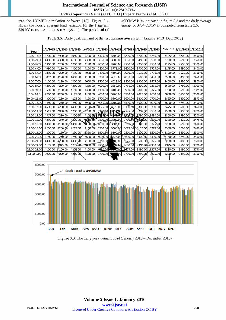
that amount lasts just one hour per year [12]. The peak

load data for the period (January 2013 – December 2013)

are tabulated as shown in table 3.5. The data are inputted






into the HOMER simulation software [13]. Figure 3.4

shows the hourly average load variation for the Nigerian

330-kV transmission lines (test system). The peak load of

4950MW is as indicated in figure 3.3 and the daily average

energy of 3754.69MW is computed from table 3.5.

Table 3.5: Daily peak demand of the test transmission system (January 2013–Dec. 2013)

Figure 3.3: The daily peak demand load (January 2013 – December 2013)

Hour1/1/2013 1/2/2013 1/3/2013 1/4/2013 1/5/2013 1/6/2013 1/7/2013 1/8/2013 1/9/2013 1/10/2013 1/11/2013 1/12/2013

0.00-1.00 4200.00 3900.00 4050.00 4200.00 4120.00 3700.00 3800.00 3700.00 3250.00 3425.00 3200.00 3450.00

1.00-2.00 4300.00 4350.00 4100.00 4350.00 3650.00 3600.00 3650.00 3450.00 3500.00 3200.00 3650.00 3650.00

2.00-3.00 4310.00 4200.00 4200.00 4170.00 3000.00 3700.00 3700.00 3250.00 3550.00 3275.00 3550.00 3500.00

3.00-4.00 4950.00 4150.00 4300.00 4100.00 2800.00 3775.00 3600.00 3500.00 3725.00 3175.00 3650.00 3400.00

4.00-5.00 3850.00 4250.00 4150.00 4050.00 3400.00 4100.00 3900.00 3575.00 3750.00 3400.00 3525.00 3500.00

5.00-6.00 3852.00 4170.00 4400.00 4100.00 3300.00 4025.00 4050.00 3600.00 3450.00 3500.00 3350.00 3450.00

6.00-7.00 4100.00 4120.00 4300.00 4070.00 3700.00 4025.00 3800.00 3900.00 3475.00 3400.00 3450.00 3300.00

7.00-8.00 4250.00 4200.00 4250.00 4250.00 4000.00 3850.00 3750.00 3800.00 3350.00 3600.00 3750.00 2900.00

8.00-9.00 3550.00 4150.00 4150.00 4350.00 4100.00 4100.00 3900.00 3800.00 3375.00 3700.00 3650.00 2875.00

9.0 - 10.0 4200.00 4290.00 4175.00 4100.00 4050.00 3700.00 3700.00 4025.00 2600.00 3800.00 3550.00 2900.00

10.00- 11.00 4300.00 4230.00 4275.00 4150.00 3700.00 3900.00 3600.00 3800.00 2700.00 3825.00 3450.00 2875.00

11.00-12.00 4450.00 4250.00 4250.00 3900.00 4050.00 3700.00 3500.00 3000.00 3000.00 3600.00 3750.00 3400.00

12.00-13.00 4500.00 4200.00 4400.00 4150.00 4075.00 4025.00 3100.00 3300.00 3300.00 3475.00 3500.00 3450.00

13.00-14.00 4517.60 4050.00 4200.00 4250.00 4200.00 3750.00 3725.00 3200.00 3550.00 3550.00 3850.00 3700.00

14.00-15.00 4517.00 4250.00 4300.00 4100.00 3850.00 4200.00 3500.00 3750.00 3450.00 3300.00 3650.00 3200.00

15.00-16.00 4250.00 4270.00 4100.00 3600.00 3800.00 3600.00 3700.00 3000.00 3500.00 3350.00 3825.00 3475.00

16.00-17.00 4300.00 4150.00 4350.00 4100.00 4000.00 3200.00 3750.00 3200.00 3325.00 3250.00 3650.00 3400.00

17.00-18.00 4250.00 4200.00 4275.00 4150.00 3700.00 3300.00 3675.00 3175.00 3275.00 3500.00 3700.00 3450.00

18.00-19.00 4220.00 4150.00 4250.00 3850.00 3900.00 3300.00 2500.00 3200.00 3500.00 3100.00 3450.00 3500.00

19.00-20.00 4150.00 4250.00 4250.00 3600.00 4000.00 3525.00 3600.00 3300.00 3400.00 3150.00 3750.00 3550.00

20.00-21.00 4300.00 4200.00 4300.00 4100.00 3750.00 3700.00 3525.00 3500.00 3375.00 3200.00 3900.00 3600.00

21.00-22.00 4125.00 4025.00 4225.00 4000.00 3800.00 3650.00 3600.00 3450.00 3350.00 3275.00 3600.00 3700.00

22.00-23.00 4100.00 4100.00 4275.00 4100.00 4050.00 3600.00 3675.00 3350.00 3375.00 3250.00 3350.00 3750.00

23.00-0.00 3900.00 4050.00 4200.00 4120.00 3700.00 3800.00 3700.00 3250.00 3425.00 3200.00 3450.00 3300.00






Figure 5: The monthly average load plot (January 2013 – December 2013)

From the result obtained in the simulation of peak load and

average load under peak transmission line (test system) for

January 2013 – December 2013, the total loss is obtained

as follows: The daily load factor is given based on hourly

load reading as

Daily load Factor (DLF) = 𝐴𝑣𝑒𝑟𝑎𝑔𝑒 𝑙𝑜𝑎𝑑 𝑖𝑛 24ℎ

𝑃𝑒𝑎𝑘 𝑙𝑜𝑎𝑑 𝑖𝑛 24ℎ 3.2

Load factor may be given for a day, a month, or a year.

The yearly or annual LF is the most useful since a year

represents a full cycle of time. Thus, the annual LF is

given as

Annual load Factor (ALF) = 𝑡𝑜𝑡𝑎𝑙 𝑎𝑛𝑛𝑢𝑎𝑙 𝑒𝑛𝑒𝑟𝑔𝑦

𝑃𝑒𝑎𝑘 𝑙𝑜𝑎𝑑 ×8760 ℎ𝑟3.3

In this study, the annual load factor (ALF) is estimated

from the average load by using the hourly average load

variation for January 2013 – December 2013.

Thus, the ALF is obtained as

ALF = DLF RAD RAM [14] 3.4 3.4

Where

ALF = Annual Load Factor

DLF = Daily load Factor

RAD = 𝐴𝑣𝑒𝑟𝑎𝑔𝑒 𝑑𝑎𝑖𝑙𝑦 𝑝𝑒𝑎𝑘 𝑙𝑜𝑎𝑑

𝑀𝑜𝑛𝑡 ℎ𝑙𝑦 𝑃𝑒𝑎𝑘 𝑙𝑜𝑎𝑑 3.5

RAM = 𝐴𝑣𝑒𝑟𝑎𝑔𝑒 𝑚𝑜𝑛𝑡 ℎ𝑙𝑦 𝑝𝑒𝑎𝑘 𝑙𝑜𝑎𝑑

𝐴𝑛𝑛𝑢𝑎𝑙 𝑃𝑒𝑎𝑘 𝑙𝑜𝑎𝑑 3.6

From the hourly readings of table 6, the peak load is

4950MW as indicated in figure 4 and daily average load is

3754.69 as calculated from table 3.5

Using equation 3.2 above, DLF is

DLF = 𝐴𝑣𝑒𝑟𝑎𝑔𝑒 𝑙𝑜𝑎𝑑 𝑖𝑛 24ℎ

𝑃𝑒𝑎𝑘 𝑙𝑜𝑎𝑑 𝑖𝑛 24ℎ =

3754 .69

4950= 0.759

The average daily peak load for January – December 2013

is 3812.08MW with monthly peak load of 4950MW in

January.

Thus, using equation 3.5

RAD = 3812.08/4950 = 0.770

Also from figure 3.4,

The average monthly peak load = 4400MW and the annual

peak load = 4950MW.

Thus, using equation 6; RAM = 4400/4950 = 0.889

Therefore, using equation 4.3, annual load factor (ALF) is

given as

ALF = 0.759 × 0.770 × 0.889 = 0.52

The Load Loss Factor (LLF) required for annual energy

calculation is given as

LLF = K ALF + (1−K) (ALF)2 [15] 3. 7

where K means proportioning multiplier in the LLF

equation 7;

where 0˂K˂ 1 and K is normally 0.3 for transmission line.






Using equation 3.7;

LLF = 0.3 (0.52) + 0.7 (0.52)2 = 0.345

Using the Loss Load Factor (LLF) of 0.345, the annual

energy for the three categories of power loss evaluated in

this study can be estimated as

Annual MWH Loss for 146.73MW (Low Power Loss

Level):

= LLF (peak loss in MW) 8760. 3. 8

Using the maximum power loss of 146.73MW obtained in

the course of this work; the total energy loss for year 2013

is estimated as

= 0.345 × 146.73 × 8760

= 443447.41MWH or 443.45GWH

Annual MWH Loss for 323.24MW (Medium Power

Loss Level):

Using equation 8 and the maximum power loss of

323.24MW obtained in the course of this work as medium

power loss level; the total energy loss for the year 2013 is

estimated as

= 0.345 × 323.24 × 8760

= 976895.93MWH or 976.895GWH

Annual MWH Loss for 738.28MW ( High Power

Loss Level):

Using equation 8 and the maximum power loss of

738.28MW obtained in the course of this work as high

power loss level; the total energy Loss for the year 2013 is

estimated as

= 0.345 × 738.28 × 8760

= 2231229.82MWH or 2231.230GWH

3.5. Cost Implications

The total amount of financial loss in the estimated annual

energy loss of section 3.4 is evaluated for each of the

power loss levels – Low, Medium and High power losses.

The cost evaluation is based on the Naira/KWH energy

rates for Eko district, under the new power tariff MYTO 2

for 2013/2014 [16]. The cost of energy is rated at N19 per

KWH or N19000/MWH, by taking the average of all the

tariff class energy unit costs (N/KWH). Using the

N19000/MWH, the annual financial loss due to each

power loss level associated with the 330-kV power lines is

estimated as follows:

For the Low Power Line Loss with annual loss of

443447.41MWH, the annual financial loss for the year

2013 is 443447.41MWH N19000/MWH

i.e. N8, 425,500,790; approximately amounted to 8.4

billion Naira

For the Medium Power Line Loss with annual loss of


2013 is 976895.93MWH N19000/MWH

i.e. N1.86 ×1010

; approximately amounted to18.6 billion

Naira

For the Low power line loss with annual loss of


2013 is 2231229.82MWH N19000MWH

i.e. N4.24 × 1010

; approximately amounted to 42.4 billion

Naira

4. Conclusion

In this study, the evaluation of technical losses-steady and

transient phenomena was captured successfully on Nigeria

330-kV transmission network. Three levels (i.e low,

medium and high) of maximum line current were

determined and used accordingly to calculate the three

categories of power loss level associated with the network

which in turn was used to estimate the annual power line

losses for the year 2013 using the peak load data for the

period (January2013 – December2013). The annual loss

energy for the year 2013 and the huge financial drain in

the network were identified and quantified;the low,

medium and high energy losses were respectively found to

be 443.45GWH, 976.895GWH and

2231.230GWHamounting to financial losses of N8.4

billion, N18.6 billion and N42.4 billion respectively.

The results of the load-flow analysis that were performed

using MATLAB and PWS compared favourably well with

the 146.73MW power loss obtained at steady-state in this

work. Also, it validated the results of 2231.23GWH losses

obtained in the work with the normal practice of PHCN

energy balance (as shown in table 2.1)thereby closing the

gap between the practical information and the theoretical

one and also it optimizes the loss level which results in a

high degree of accuracy.

Acknowledgement

The author is highly indebted to Power Holding Company

of Nigeria (PHCN) for providing relevant data necessary

for power-flow study and the peak load demand data for

the period (January 2013-December 2013.

References

[1] PHCH, 2003National Control Centre Oshogbo.(2004).

Generation and Transmission GridOperations.

AnnualTechnical Report for 2003.

[2] PHCN National Control Centre Oshogbo.

(2005).Generation and Transmission Grid

Operations.Annual Technical for Report 2004.

[3] Pabia, A. S., 2013. Electric Power Distribution (4th

Edition), 6th; Reprint, Tata McGraw-Hill Publication

Com. Ltd. New Delhi

[4] IEA (2013), Key World Energy Statistics

s2013[online] available:






http://www.iea.org/publications/freepublications/publi

cation/KeyWorld2013.pdfaccessed 31/05/2014

[5] Gaspar, Viera (2011). "Electrical Annual

EnergyLosses Determination in Low Voltage -

ACaseStudy". RevistaEletronica Sistemas &

Gestao,91-116 vol. 6.

[6] Wadwah, C. (2006). Electric Power system.Chennai:

New Age International Publisher Limited.

[7] Glover, J. D and Sarma, 2002. Power System Analysis

and Design. (3rd

Edition), Wadsworth Group, Brooks

Cole,a division of Thomson Learning Centre

[8] ONEM. (2011). "The Electricity market Operations,

January - December 2010" theMarketOperations

report. Transmission Company of Nigeria.

[9] PHCN NCC ANNUAL REPORT. (2009). Generation,

Transmission and Distribution Grid Operations.

National Control Centre (NCC) Oshogbo.

[10] Power Holding Company of Nigeria (PHCN). (2013).

"Network Data of the Nigerian 28-bus Power System;

National Control Centre (NCC)". Oshogbo.

[11] Power World Co-operation. ((2014 Version)). Power

World Simulator, Version 18 Glover/Sarma

Build11/02/01, Licensed only forEvaluation and

University Education use.

[12] Lowel. (2006). Energy Utility Rate Setting . Retrieved

June 25th, 2013, from ulu.com.p.66.ISBN

1411689593 :

[13] HOMER Pro 3.1. (n.d.). National Renewable Energy

Laboratory (NREL)Retrieved from617 Cole

Boulevard Golden, CO 80401-3393:

http:/www.nrel.gov/homer

[14] IEEE Standard Board. (1997). "IEEE

RecommendedPractice for Industrial and Commercial

Power SystemsAnalysis". Approved by American

National Standard Institute, (IEEE Std 399-1991).

[15] Electricity Authority, Te Mana Hiko. (2013).Annual

Energy Report .www.parliament.nz/.../electricity-

authority-te-mana-hiko-annual-report-2...

[16] PHCN Eko Distribution Company. (2013/2014,

February 3rd). 2013 New Energy Tariff &Cost for

EkoDistrict. Retrieved February 16th, 2014, from

Power Tariff under MYTO 2 for 2013/2014


on the cost implications of technical energy losses on

Documents