Real-Time Human Pose Recognition in Parts from Single Depth Images

Jamie Shotton Andrew Fitzgibbon Mat Cook Toby Sharp Mark FinocchioRichard Moore Alex Kipman Andrew Blake

Microsoft Research Cambridge & Xbox Incubation

AbstractWe propose a new method to quickly and accurately pre-

dict 3D positions of body joints from a single depth image,using no temporal information. We take an object recog-nition approach, designing an intermediate body parts rep-resentation that maps the difficult pose estimation probleminto a simpler per-pixel classification problem. Our largeand highly varied training dataset allows the classifier toestimate body parts invariant to pose, body shape, clothing,etc. Finally we generate confidence-scored 3D proposals ofseveral body joints by reprojecting the classification resultand finding local modes.

The system runs at 200 frames per second on consumerhardware. Our evaluation shows high accuracy on bothsynthetic and real test sets, and investigates the effect of sev-eral training parameters. We achieve state of the art accu-racy in our comparison with related work and demonstrateimproved generalization over exact whole-skeleton nearestneighbor matching.

1. IntroductionRobust interactive human body tracking has applica-

tions including gaming, human-computer interaction, secu-rity, telepresence, and even health-care. The task has re-cently been greatly simplified by the introduction of real-time depth cameras [16, 19, 44, 37, 28, 13]. However, eventhe best existing systems still exhibit limitations. In partic-ular, until the launch of Kinect [21], none ran at interactiverates on consumer hardware while handling a full range ofhuman body shapes and sizes undergoing general body mo-tions. Some systems achieve high speeds by tracking fromframe to frame but struggle to re-initialize quickly and soare not robust. In this paper, we focus on pose recognitionin parts: detecting from a single depth image a small set of3D position candidates for each skeletal joint. Our focus onper-frame initialization and recovery is designed to comple-ment any appropriate tracking algorithm [7, 39, 16, 42, 13]that might further incorporate temporal and kinematic co-herence. The algorithm presented here forms a core com-ponent of the Kinect gaming platform [21].

Illustrated in Fig. 1 and inspired by recent object recog-nition work that divides objects into parts (e.g. [12, 43]),our approach is driven by two key design goals: computa-tional efficiency and robustness. A single input depth imageis segmented into a dense probabilistic body part labeling,with the parts defined to be spatially localized near skeletal

CVPR Teaser seq 1: frame 15

seq 2: frame 236 seq 5: take 1, 72

depth image body parts 3D joint proposals

Figure 1. Overview. From an single input depth image, a per-pixelbody part distribution is inferred. (Colors indicate the most likelypart labels at each pixel, and correspond in the joint proposals).Local modes of this signal are estimated to give high-quality pro-posals for the 3D locations of body joints, even for multiple users.

joints of interest. Reprojecting the inferred parts into worldspace, we localize spatial modes of each part distributionand thus generate (possibly several) confidence-weightedproposals for the 3D locations of each skeletal joint.

We treat the segmentation into body parts as a per-pixelclassification task (no pairwise terms or CRF have provednecessary). Evaluating each pixel separately avoids a com-binatorial search over the different body joints, althoughwithin a single part there are of course still dramatic dif-ferences in the contextual appearance. For training data,we generate realistic synthetic depth images of humans ofmany shapes and sizes in highly varied poses sampled froma large motion capture database. We train a deep ran-domized decision forest classifier which avoids overfittingby using hundreds of thousands of training images. Sim-ple, discriminative depth comparison image features yield3D translation invariance while maintaining high computa-tional efficiency. For further speed, the classifier can be runin parallel on each pixel on a GPU [34]. Finally, spatialmodes of the inferred per-pixel distributions are computedusing mean shift [10] resulting in the 3D joint proposals.

An optimized implementation of our algorithm runs inunder 5ms per frame (200 frames per second) on the Xbox360 GPU, at least one order of magnitude faster than exist-ing approaches. It works frame-by-frame across dramati-cally differing body shapes and sizes, and the learned dis-criminative approach naturally handles self-occlusions and

1

poses cropped by the image frame. We evaluate on both realand synthetic depth images, containing challenging poses ofa varied set of subjects. Even without exploiting temporalor kinematic constraints, the 3D joint proposals are both ac-curate and stable. We investigate the effect of several train-ing parameters and show how very deep trees can still avoidoverfitting due to the large training set. We demonstratethat our part proposals generalize at least as well as exactnearest-neighbor in both an idealized and realistic setting,and show a substantial improvement over the state of theart. Further, results on silhouette images suggest more gen-eral applicability of our approach.

Our main contribution is to treat pose estimation as ob-ject recognition using a novel intermediate body parts rep-resentation designed to spatially localize joints of interestat low computational cost and high accuracy. Our experi-ments also carry several insights: (i) synthetic depth train-ing data is an excellent proxy for real data; (ii) scaling upthe learning problem with varied synthetic data is importantfor high accuracy; and (iii) our parts-based approach gener-alizes better than even an oracular exact nearest neighbor.

Related Work. Human pose estimation has generated avast literature (surveyed in [22, 29]). The recent availabilityof depth cameras has spurred further progress [16, 19, 28].Grest et al. [16] use Iterated Closest Point to track a skele-ton of a known size and starting position. Anguelov et al.[3] segment puppets in 3D range scan data into head, limbs,torso, and background using spin images and a MRF. In[44], Zhu & Fujimura build heuristic detectors for coarseupper body parts (head, torso, arms) using a linear program-ming relaxation, but require a T-pose initialization to sizethe model. Siddiqui & Medioni [37] hand craft head, hand,and forearm detectors, and show data-driven MCMC modelfitting outperforms ICP. Kalogerakis et al. [18] classify andsegment vertices in a full closed 3D mesh into differentparts, but do not deal with occlusions and are sensitive tomesh topology. Most similar to our approach, Plagemannet al. [28] build a 3D mesh to find geodesic extrema inter-est points which are classified into 3 parts: head, hand, andfoot. Their method provides both a location and orientationestimate of these parts, but does not distinguish left fromright and the use of interest points limits the choice of parts.

Advances have also been made using conventional in-tensity cameras, though typically at much higher computa-tional cost. Bregler & Malik [7] track humans using twistsand exponential maps from a known initial pose. Ioffe &Forsyth [17] group parallel edges as candidate body seg-ments and prune combinations of segments using a pro-jected classifier. Mori & Malik [24] use the shape con-text descriptor to match exemplars. Ramanan & Forsyth[31] find candidate body segments as pairs of parallel lines,clustering appearances across frames. Shakhnarovich et al.[33] estimate upper body pose, interpolating k-NN poses

matched by parameter sensitive hashing. Agarwal & Triggs[1] learn a regression from kernelized image silhouettes fea-tures to pose. Sigal et al. [39] use eigen-appearance tem-plate detectors for head, upper arms and lower legs pro-posals. Felzenszwalb & Huttenlocher [11] apply pictorialstructures to estimate pose efficiently. Navaratnam et al.[25] use the marginal statistics of unlabeled data to im-prove pose estimation. Urtasun & Darrel [41] proposed alocal mixture of Gaussian Processes to regress human pose.Auto-context was used in [40] to obtain a coarse body partlabeling but this was not defined to localize joints and clas-sifying each frame took about 40 seconds. Rogez et al. [32]train randomized decision forests on a hierarchy of classesdefined on a torus of cyclic human motion patterns and cam-era angles. Wang & Popovic [42] track a hand clothed in acolored glove. Our system could be seen as automaticallyinferring the colors of an virtual colored suit from a depthimage. Bourdev & Malik [6] present ‘poselets’ that formtight clusters in both 3D pose and 2D image appearance,detectable using SVMs.

2. DataPose estimation research has often focused on techniques

to overcome lack of training data [25], because of two prob-lems. First, generating realistic intensity images using com-puter graphics techniques [33, 27, 26] is hampered by thehuge color and texture variability induced by clothing, hair,and skin, often meaning that the data are reduced to 2D sil-houettes [1]. Although depth cameras significantly reducethis difficulty, considerable variation in body and clothingshape remains. The second limitation is that synthetic bodypose images are of necessity fed by motion-capture (mocap)data. Although techniques exist to simulate human motion(e.g. [38]) they do not yet produce the range of volitionalmotions of a human subject.

In this section we review depth imaging and show howwe use real mocap data, retargetted to a variety of base char-acter models, to synthesize a large, varied dataset. We be-lieve this dataset to considerably advance the state of the artin both scale and variety, and demonstrate the importanceof such a large dataset in our evaluation.2.1. Depth imaging

Depth imaging technology has advanced dramaticallyover the last few years, finally reaching a consumer pricepoint with the launch of Kinect [21]. Pixels in a depth imageindicate calibrated depth in the scene, rather than a measureof intensity or color. We employ the Kinect camera whichgives a 640x480 image at 30 frames per second with depthresolution of a few centimeters.

Depth cameras offer several advantages over traditionalintensity sensors, working in low light levels, giving a cali-brated scale estimate, being color and texture invariant, andresolving silhouette ambiguities in pose. They also greatly

Training & Test Data

syn

thet

ic (

trai

n &

te

st)

real

(te

st)

syn

thet

ic (

trai

n &

te

st)

real

(te

st)

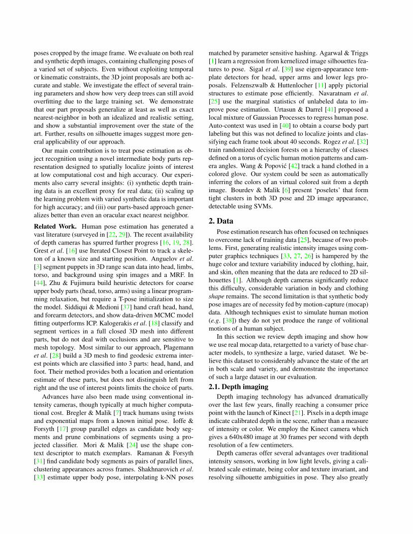
Figure 2. Synthetic and real data. Pairs of depth image and ground truth body parts. Note wide variety in pose, shape, clothing, and crop.

simplify the task of background subtraction which we as-sume in this work. But most importantly for our approach,it is straightforward to synthesize realistic depth images ofpeople and thus build a large training dataset cheaply.

2.2. Motion capture dataThe human body is capable of an enormous range of

poses which are difficult to simulate. Instead, we capture alarge database of motion capture (mocap) of human actions.Our aim was to span the wide variety of poses people wouldmake in an entertainment scenario. The database consists ofapproximately 500k frames in a few hundred sequences ofdriving, dancing, kicking, running, navigating menus, etc.

We expect our semi-local body part classifier to gener-alize somewhat to unseen poses. In particular, we need notrecord all possible combinations of the different limbs; inpractice, a wide range of poses proves sufficient. Further,we need not record mocap with variation in rotation aboutthe vertical axis, mirroring left-right, scene position, bodyshape and size, or camera pose, all of which can be addedin (semi-)automatically.

Since the classifier uses no temporal information, weare interested only in static poses and not motion. Often,changes in pose from one mocap frame to the next are sosmall as to be insignificant. We thus discard many similar,redundant poses from the initial mocap data using ‘furthestneighbor’ clustering [15] where the distance between posesp1 and p2 is defined as maxj ‖pj1−p

j2‖2, the maximum Eu-

clidean distance over body joints j. We use a subset of 100kposes such that no two poses are closer than 5cm.

We have found it necessary to iterate the process of mo-tion capture, sampling from our model, training the classi-fier, and testing joint prediction accuracy in order to refinethe mocap database with regions of pose space that had beenpreviously missed out. Our early experiments employedthe CMU mocap database [9] which gave acceptable resultsthough covered far less of pose space.

2.3. Generating synthetic dataWe build a randomized rendering pipeline from which

we can sample fully labeled training images. Our goals inbuilding this pipeline were twofold: realism and variety. Forthe learned model to work well, the samples must closelyresemble real camera images, and contain good coverage of

the appearance variations we hope to recognize at test time.While depth/scale and translation variations are handled ex-plicitly in our features (see below), other invariances cannotbe encoded efficiently. Instead we learn invariance from thedata to camera pose, body pose, and body size and shape.

The synthesis pipeline first randomly samples a set ofparameters, and then uses standard computer graphics tech-niques to render depth and (see below) body part imagesfrom texture mapped 3D meshes. The mocap is retarget-ting to each of 15 base meshes spanning the range of bodyshapes and sizes, using [4]. Further slight random vari-ation in height and weight give extra coverage of bodyshapes. Other randomized parameters include the mocapframe, camera pose, camera noise, clothing and hairstyle.We provide more details of these variations in the supple-mentary material. Fig. 2 compares the varied output of thepipeline to hand-labeled real camera images.

3. Body Part Inference and Joint ProposalsIn this section we describe our intermediate body parts

representation, detail the discriminative depth image fea-tures, review decision forests and their application to bodypart recognition, and finally discuss how a mode finding al-gorithm is used to generate joint position proposals.

3.1. Body part labelingA key contribution of this work is our intermediate body

part representation. We define several localized body partlabels that densely cover the body, as color-coded in Fig. 2.Some of these parts are defined to directly localize partic-ular skeletal joints of interest, while others fill the gaps orcould be used in combination to predict other joints. Our in-termediate representation transforms the problem into onethat can readily be solved by efficient classification algo-rithms; we show in Sec. 4.3 that the penalty paid for thistransformation is small.

The parts are specified in a texture map that is retargettedto skin the various characters during rendering. The pairs ofdepth and body part images are used as fully labeled data forlearning the classifier (see below). For the experiments inthis paper, we use 31 body parts: LU/RU/LW/RW head, neck,L/R shoulder, LU/RU/LW/RW arm, L/R elbow, L/R wrist, L/Rhand, LU/RU/LW/RW torso, LU/RU/LW/RW leg, L/R knee,L/R ankle, L/R foot (Left, Right, Upper, loWer). Distinct

(a)

body parts

Image Features

(b)

𝜃2

𝜃1

𝜃2

𝜃2

𝜃1

𝜃2

Figure 3. Depth image features. The yellow crosses indicates thepixel x being classified. The red circles indicate the offset pixelsas defined in Eq. 1. In (a), the two example features give a largedepth difference response. In (b), the same two features at newimage locations give a much smaller response.

parts for left and right allow the classifier to disambiguatethe left and right sides of the body.

Of course, the precise definition of these parts could bechanged to suit a particular application. For example, in anupper body tracking scenario, all the lower body parts couldbe merged. Parts should be sufficiently small to accuratelylocalize body joints, but not too numerous as to waste ca-pacity of the classifier.

3.2. Depth image featuresWe employ simple depth comparison features, inspired

by those in [20]. At a given pixel x, the features compute

fθ(I,x) = dI

(x+

u

dI(x)

)− dI

(x+

v

dI(x)

), (1)

where dI(x) is the depth at pixel x in image I , and parame-ters θ = (u,v) describe offsets u and v. The normalizationof the offsets by 1

dI(x)ensures the features are depth invari-

ant: at a given point on the body, a fixed world space offsetwill result whether the pixel is close or far from the camera.The features are thus 3D translation invariant (modulo per-spective effects). If an offset pixel lies on the backgroundor outside the bounds of the image, the depth probe dI(x′)is given a large positive constant value.

Fig. 3 illustrates two features at different pixel locationsx. Feature fθ1 looks upwards: Eq. 1 will give a large pos-itive response for pixels x near the top of the body, but avalue close to zero for pixels x lower down the body. Fea-ture fθ2 may instead help find thin vertical structures suchas the arm.

Individually these features provide only a weak signalabout which part of the body the pixel belongs to, but incombination in a decision forest they are sufficient to accu-rately disambiguate all trained parts. The design of thesefeatures was strongly motivated by their computational effi-ciency: no preprocessing is needed; each feature need onlyread at most 3 image pixels and perform at most 5 arithmeticoperations; and the features can be straightforwardly imple-mented on the GPU. Given a larger computational budget,one could employ potentially more powerful features basedon, for example, depth integrals over regions, curvature, orlocal descriptors e.g. [5].

Random Forests

… tree 1 tree 𝑇

(𝐼, x) (𝐼, x)

𝑃𝑇(𝑐) 𝑃1(𝑐)

Figure 4. Randomized Decision Forests. A forest is an ensembleof trees. Each tree consists of split nodes (blue) and leaf nodes(green). The red arrows indicate the different paths that might betaken by different trees for a particular input.

3.3. Randomized decision forestsRandomized decision trees and forests [35, 30, 2, 8] have

proven fast and effective multi-class classifiers for manytasks [20, 23, 36], and can be implemented efficiently on theGPU [34]. As illustrated in Fig. 4, a forest is an ensembleof T decision trees, each consisting of split and leaf nodes.Each split node consists of a feature fθ and a threshold τ .To classify pixel x in image I , one starts at the root and re-peatedly evaluates Eq. 1, branching left or right accordingto the comparison to threshold τ . At the leaf node reachedin tree t, a learned distribution Pt(c|I,x) over body part la-bels c is stored. The distributions are averaged together forall trees in the forest to give the final classification

P (c|I,x) = 1

T

T∑t=1

Pt(c|I,x) . (2)

Training. Each tree is trained on a different set of randomlysynthesized images. A random subset of 2000 example pix-els from each image is chosen to ensure a roughly even dis-tribution across body parts. Each tree is trained using thefollowing algorithm [20]:

1. Randomly propose a set of splitting candidates φ =(θ, τ) (feature parameters θ and thresholds τ ).

2. Partition the set of examples Q = {(I,x)} into leftand right subsets by each φ:

Ql(φ) = { (I,x) | fθ(I,x) < τ } (3)Qr(φ) = Q \Ql(φ) (4)

3. Compute the φ giving the largest gain in information:

φ? = argmaxφ

G(φ) (5)

G(φ) = H(Q)−∑

s∈{l,r}

|Qs(φ)||Q|

H(Qs(φ)) (6)

where Shannon entropyH(Q) is computed on the nor-malized histogram of body part labels lI(x) for all(I,x) ∈ Q.

4. If the largest gain G(φ?) is sufficient, and the depth inthe tree is below a maximum, then recurse for left andright subsets Ql(φ

?) and Qr(φ?).

• depth, map, front/right/top • pose, distances, cropping, camera angles, body size and shape (e.g. small child, thin/fat), • failure modes: underlying probability correct, can detect failures with confidence • synthetic / real / failures

Example inferences

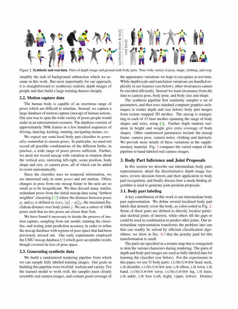
Figure 5. Example inferences. Synthetic (top row); real (middle); failure modes (bottom). Left column: ground truth for a neutral pose asa reference. In each example we see the depth image, the inferred most likely body part labels, and the joint proposals show as front, right,and top views (overlaid on a depth point cloud). Only the most confident proposal for each joint above a fixed, shared threshold is shown.

To keep the training times down we employ a distributedimplementation. Training 3 trees to depth 20 from 1 millionimages takes about a day on a 1000 core cluster.

3.4. Joint position proposalsBody part recognition as described above infers per-pixel

information. This information must now be pooled acrosspixels to generate reliable proposals for the positions of 3Dskeletal joints. These proposals are the final output of ouralgorithm, and could be used by a tracking algorithm to self-initialize and recover from failure.

A simple option is to accumulate the global 3D centersof probability mass for each part, using the known cali-brated depth. However, outlying pixels severely degradethe quality of such a global estimate. Instead we employ alocal mode-finding approach based on mean shift [10] witha weighted Gaussian kernel.

We define a density estimator per body part as

fc(x) ∝N∑i=1

wic exp

(−∥∥∥∥ x− xi

bc

∥∥∥∥2), (7)

where x is a coordinate in 3D world space, N is the numberof image pixels, wic is a pixel weighting, xi is the reprojec-tion of image pixel xi into world space given depth dI(xi),and bc is a learned per-part bandwidth. The pixel weightingwic considers both the inferred body part probability at thepixel and the world surface area of the pixel:

wic = P (c|I,xi) · dI(xi)2 . (8)

This ensures density estimates are depth invariant and gavea small but significant improvement in joint prediction ac-curacy. Depending on the definition of body parts, the pos-terior P (c|I,x) can be pre-accumulated over a small set ofparts. For example, in our experiments the four body partscovering the head are merged to localize the head joint.

Mean shift is used to find modes in this density effi-ciently. All pixels above a learned probability threshold λcare used as starting points for part c. A final confidence es-timate is given as a sum of the pixel weights reaching eachmode. This proved more reliable than taking the modal den-sity estimate.

The detected modes lie on the surface of the body. Eachmode is therefore pushed back into the scene by a learnedz offset ζc to produce a final joint position proposal. Thissimple, efficient approach works well in practice. The band-widths bc, probability threshold λc, and surface-to-interiorz offset ζc are optimized per-part on a hold-out validationset of 5000 images by grid search. (As an indication, thisresulted in mean bandwidth 0.065m, probability threshold0.14, and z offset 0.039m).

4. ExperimentsIn this section we describe the experiments performed to

evaluate our method. We show both qualitative and quan-titative results on several challenging datasets, and com-pare with both nearest-neighbor approaches and the stateof the art [13]. We provide further results in the supple-mentary material. Unless otherwise specified, parametersbelow were set as: 3 trees, 20 deep, 300k training imagesper tree, 2000 training example pixels per image, 2000 can-didate features θ, and 50 candidate thresholds τ per feature.Test data. We use challenging synthetic and real depth im-ages to evaluate our approach. For our synthetic test set,we synthesize 5000 depth images, together with the groundtruth body part labels and joint positions. The original mo-cap poses used to generate these images are held out fromthe training data. Our real test set consists of 8808 frames ofreal depth images over 15 different subjects, hand-labeledwith dense body parts and 7 upper body joint positions. Wealso evaluate on the real depth data from [13]. The resultssuggest that effects seen on synthetic data are mirrored inthe real data, and further that our synthetic test set is by farthe ‘hardest’ due to the extreme variability in pose and bodyshape. For most experiments we limit the rotation of theuser to ±120◦ in both training and synthetic test data sincethe user is facing the camera (0◦) in our main entertainmentscenario, though we also evaluate the full 360◦ scenario.Error metrics. We quantify both classification and jointprediction accuracy. For classification, we report the av-erage per-class accuracy, i.e. the average of the diagonal ofthe confusion matrix between the ground truth part label andthe most likely inferred part label. This metric weights each

30%

35%

40%

45%

50%

55%

60%

0 100 200 300

Ave

rage

per

-cla

ss a

ccu

racy

Maximum probe offset (pixel meters)

Real test data

Synthetic test data

Combined Results

30%

35%

40%

45%

50%

55%

60%

5 10 15 20Depth of trees

Real Test Set

900k training images

15k training images

(a) (b) (c)

10%

20%

30%

40%

50%

60%

10 1000 100000

Ave

rage

per

-cla

ss a

ccu

racy

Num. training images (log scale)

Synthetic test setReal test setSilhouette (scale)Silhouette (no scale)

30%

35%

40%

45%

50%

55%

60%

8 12 16 20

Ave

rage

per

-cla

ss a

ccu

racy

Depth of trees

Synthetic Test Set

900k training images

15k training images

Figure 6. Training parameters vs. classification accuracy. (a) Number of training images. (b) Depth of trees. (c) Maximum probe offset.

body part equally despite their varying sizes, though misla-belings on the part boundaries reduce the absolute numbers.

For joint proposals, we generate recall-precision curvesas a function of confidence threshold. We quantify accuracyas average precision per joint, or mean average precision(mAP) over all joints.The first joint proposal within D me-ters of the ground truth position is taken as a true positive,while other proposals also within D meters count as falsepositives. This penalizes multiple spurious detections nearthe correct position which might slow a downstream track-ing algorithm. Any joint proposals outside D meters alsocount as false positives. Note that all proposals (not just themost confident) are counted in this metric. Joints invisiblein the image are not penalized as false negatives. We setD = 0.1m below, approximately the accuracy of the hand-labeled real test data ground truth. The strong correlationof classification and joint prediction accuracy (c.f . the bluecurves in Figs. 6(a) and 8(a)) suggests the trends observedbelow for one also apply for the other.

4.1. Qualitative resultsFig. 5 shows example inferences of our algorithm. Note

high accuracy of both classification and joint predictionacross large variations in body and camera pose, depth inscene, cropping, and body size and shape (e.g. small childvs. heavy adult). The bottom row shows some failure modesof the body part classification. The first example showsa failure to distinguish subtle changes in the depth imagesuch as the crossed arms. Often (as with the second andthird failure examples) the most likely body part is incor-rect, but there is still sufficient correct probability mass indistribution P (c|I,x) that an accurate proposal can still begenerated. The fourth example shows a failure to generalizewell to an unseen pose, but the confidence gates bad propos-als, maintaining high precision at the expense of recall.

Note that no temporal or kinematic constraints (otherthan those implicit in the training data) are used for anyof our results. Despite this, per-frame results on video se-quences in the supplementary material show almost everyjoint accurately predicted with remarkably little jitter.

4.2. Classification accuracyWe investigate the effect of several training parameters

on classification accuracy. The trends are highly correlatedbetween the synthetic and real test sets, and the real testset appears consistently ‘easier’ than the synthetic test set,probably due to the less varied poses present.Number of training images. In Fig. 6(a) we show howtest accuracy increases approximately logarithmically withthe number of randomly generated training images, thoughstarts to tail off around 100k images. As shown below, thissaturation is likely due to the limited model capacity of a 3tree, 20 deep decision forest.Silhouette images. We also show in Fig. 6(a) the qualityof our approach on synthetic silhouette images, where thefeatures in Eq. 1 are either given scale (as the mean depth)or not (a fixed constant depth). For the corresponding jointprediction using a 2D metric with a 10 pixel true positivethreshold, we got 0.539 mAP with scale and 0.465 mAPwithout. While clearly a harder task due to depth ambigui-ties, these results suggest the applicability of our approachto other imaging modalities.Depth of trees. Fig. 6(b) shows how the depth of trees af-fects test accuracy using either 15k or 900k images. Of allthe training parameters, depth appears to have the most sig-nificant effect as it directly impacts the model capacity ofthe classifier. Using only 15k images we observe overfittingbeginning around depth 17, but the enlarged 900k trainingset avoids this. The high accuracy gradient at depth 20 sug-gests even better results can be achieved by training stilldeeper trees, at a small extra run-time computational costand a large extra memory penalty. Of practical interest isthat, until about depth 10, the training set size matters little,suggesting an efficient training strategy.Maximum probe offset. The range of depth probe offsetsallowed during training has a large effect on accuracy. Weshow this in Fig. 6(c) for 5k training images, where ‘maxi-mum probe offset’ means the max. absolute value proposedfor both x and y coordinates of u and v in Eq. 1. The con-centric boxes on the right show the 5 tested maximum off-

Joint prediction accuracy

0.00.10.20.30.40.50.60.70.80.91.0

Cen

ter

Hea

d

Cen

ter

Nec

k

Left

Sh

ou

lde

r

Rig

ht

Sho

uld

er

Left

Elb

ow

Rig

ht

Elb

ow

Left

Wri

st

Rig

ht

Wri

st

Left

Han

d

Rig

ht

Han

d

Left

Kn

ee

Rig

ht

Kn

ee

Left

An

kle

Rig

ht

An

kle

Left

Fo

ot

Rig

ht

Foo

t

Mea

n A

P

Ave

rage

pre

cisi

on

Joint prediction from ground truth body parts

Joint prediction from inferred body parts 0.3

0.4

0.5

0.6

0.7

0.8

0.9

1.0

Hea

d

Ne

ck

L. S

ho

uld

er

R. S

ho

uld

er

L. E

lbo

w

R. E

lbo

w

L. W

rist

R. W

rist

L. H

and

R. H

and

L. K

nee

R. K

nee

L. A

nkl

e

R. A

nkl

e

L. F

oo

t

R. F

oo

t

Mea

n A

P

Ave

rage

pre

cisi

on

Joint prediction from ground truth body parts

Joint prediction from inferred body parts

Figure 7. Joint prediction accuracy. We compare the actual per-formance of our system (red) with the best achievable result (blue)given the ground truth body part labels.

sets calibrated for a left shoulder pixel in that image; thelargest offset covers almost all the body. (Recall that thismaximum offset scales with world depth of the pixel). Asthe maximum probe offset is increased, the classifier is ableto use more spatial context to make its decisions, thoughwithout enough data would eventually risk overfitting to thiscontext. Accuracy increases with the maximum probe off-set, though levels off around 129 pixel meters.

4.3. Joint prediction accuracyIn Fig. 7 we show average precision results on the syn-

thetic test set, achieving 0.731 mAP. We compare an ide-alized setup that is given the ground truth body part labelsto the real setup using inferred body parts. While we dopay a small penalty for using our intermediate body partsrepresentation, for many joints the inferred results are bothhighly accurate and close to this upper bound. On the realtest set, we have ground truth labels for head, shoulders, el-bows, and hands. An mAP of 0.984 is achieved on thoseparts given the ground truth body part labels, while 0.914mAP is achieved using the inferred body parts. As expected,these numbers are considerably higher on this easier test set.Comparison with nearest neighbor. To highlight the needto treat pose recognition in parts, and to calibrate the dif-ficulty of our test set for the reader, we compare withtwo variants of exact nearest-neighbor whole-body match-ing in Fig. 8(a). The first, idealized, variant matches theground truth test skeleton to a set of training exemplar skele-tons with optimal rigid translational alignment in 3D worldspace. Of course, in practice one has no access to the testskeleton. As an example of a realizable system, the secondvariant uses chamfer matching [14] to compare the test im-age to the training exemplars. This is computed using depthedges and 12 orientation bins. To make the chamfer taskeasier, we throw out any cropped training or test images.We align images using the 3D center of mass, and foundthat further local rigid translation only reduced accuracy.

Our algorithm, recognizing in parts, generalizes betterthan even the idealized skeleton matching until about 150ktraining images are reached. As noted above, our resultsmay get even better with deeper trees, but already we ro-

bustly infer 3D body joint positions and cope naturally withcropping and translation. The speed of nearest neighborchamfer matching is also drastically slower (2 fps) than ouralgorithm. While hierarchical matching [14] is faster, onewould still need a massive exemplar set to achieve compa-rable accuracy.Comparison with [13]. The authors of [13] provided theirtest data and results for direct comparison. Their algorithmuses body part proposals from [28] and further tracks theskeleton with kinematic and temporal information. Theirdata comes from a time-of-flight depth camera with verydifferent noise characteristics to our structured light sen-sor. Without any changes to our training data or algorithm,Fig. 8(b) shows considerably improved joint prediction av-erage precision. Our algorithm also runs at least 10x faster.Full rotations and multiple people. To evaluate the full360◦ rotation scenario, we trained a forest on 900k imagescontaining full rotations and tested on 5k synthetic full ro-tation images (with held out poses). Despite the massiveincrease in left-right ambiguity, our system was still ableto achieve an mAP of 0.655, indicating that our classifiercan accurately learn the subtle visual cues that distinguishfront and back facing poses. Residual left-right uncertaintyafter classification can naturally be propagated to a track-ing algorithm through multiple hypotheses. Our approachcan propose joint positions for multiple people in the image,since the per-pixel classifier generalizes well even withoutexplicit training for this scenario. Results are given in Fig. 1and the supplementary material.Faster proposals. We also implemented a faster alterna-tive approach to generating the proposals based on simplebottom-up clustering. Combined with body part classifica-tion, this runs at ∼ 200 fps on the Xbox GPU, vs. ∼ 50 fpsusing mean shift on a modern 8 core desktop CPU. Giventhe computational savings, the 0.677 mAP achieved on thesynthetic test set compares favorably to the 0.731 mAP ofthe mean shift approach.

5. DiscussionWe have seen how accurate proposals for the 3D loca-

tions of body joints can be estimated in super real-time fromsingle depth images. We introduced body part recognitionas an intermediate representation for human pose estima-tion. Using a highly varied synthetic training set allowedus to train very deep decision forests using simple depth-invariant features without overfitting, learning invariance toboth pose and shape. Detecting modes in a density functiongives the final set of confidence-weighted 3D joint propos-als. Our results show high correlation between real and syn-thetic data, and between the intermediate classification andthe final joint proposal accuracy. We have highlighted theimportance of breaking the whole skeleton into parts, andshow state of the art accuracy on a competitive test set.

As future work, we plan further study of the variability

0.0

0.1

0.2

0.3

0.4

0.5

0.6

0.7

0.8

30 300 3000 30000 300000

Me

an a

vera

ge p

reci

sio

n

Number of training images (log scale)

Ground truth skeleton NN

Chamfer NN

Our algorithm

0.5

0.6

0.7

0.8

0.9

1.0

Hea

d

Nec

k

L. S

ho

uld

er

R. S

ho

uld

er

L. E

lbo

w

R. E

lbo

w

L. W

rist

R. W

rist

L. H

and

R. H

and

L. K

nee

R. K

nee

L. A

nkl

e

R. A

nkl

e

L. F

oo

t

R. F

oo

t

Mea

n A

P

Ave

rage

pre

cisi

on

Our result (per frame)

Ganapathi et al. (tracking)

Combined Comparisons

(a) (b)

Figure 8. Comparisons. (a) Comparison with nearest neighbor matching. (b) Comparison with [13]. Even without the kinematic andtemporal constraints exploited by [13], our algorithm is able to more accurately localize body joints.

in the source mocap data, the properties of the generativemodel underlying the synthesis pipeline, and the particularpart definitions. Whether a similarly efficient approach thatcan directly regress joint positions is also an open question.Perhaps a global estimate of latent variables such as coarseperson orientation could be used to condition the body partinference and remove ambiguities in local pose estimates.Acknowledgements. We thank the many skilled engineers inXbox, particularly Robert Craig, Matt Bronder, Craig Peeper, Momin Al-Ghosien, and Ryan Geiss, who built the Kinect tracking system on topof this research. We also thank John Winn, Duncan Robertson, AntonioCriminisi, Shahram Izadi, Ollie Williams, and Mihai Budiu for help andvaluable discussions, and Varun Ganapathi and Christian Plagemann forproviding their test data.

References[1] A. Agarwal and B. Triggs. 3D human pose from silhouettes by rele-

vance vector regression. In Proc. CVPR, 2004. 2[2] Y. Amit and D. Geman. Shape quantization and recognition with

randomized trees. Neural Computation, 9(7):1545–1588, 1997. 4[3] D. Anguelov, B. Taskar, V. Chatalbashev, D. Koller, D. Gupta, and

A. Ng. Discriminative learning of markov random fields for segmen-tation of 3D scan data. In Proc. CVPR, 2005. 2

[4] Autodesk MotionBuilder. 3[5] S. Belongie, J. Malik, and J. Puzicha. Shape matching and object

recognition using shape contexts. IEEE Trans. PAMI, 24, 2002. 4[6] L. Bourdev and J. Malik. Poselets: Body part detectors trained using

3D human pose annotations. In Proc. ICCV, 2009. 2[7] C. Bregler and J. Malik. Tracking people with twists and exponential

maps. In Proc. CVPR, 1998. 1, 2[8] L. Breiman. Random forests. Mach. Learning, 45(1):5–32, 2001. 4[9] CMU Mocap Database. http://mocap.cs.cmu.edu/. 3

[10] D. Comaniciu and P. Meer. Mean shift: A robust approach towardfeature space analysis. IEEE Trans. PAMI, 24(5), 2002. 1, 5

[11] P. Felzenszwalb and D. Huttenlocher. Pictorial structures for objectrecognition. IJCV, 61(1):55–79, Jan. 2005. 2

[12] R. Fergus, P. Perona, and A. Zisserman. Object class recognition byunsupervised scale-invariant learning. In Proc. CVPR, 2003. 1

[13] V. Ganapathi, C. Plagemann, D. Koller, and S. Thrun. Real timemotion capture using a single time-of-flight camera. In Proc. CVPR,2010. 1, 5, 7, 8

[14] D. Gavrila. Pedestrian detection from a moving vehicle. In Proc.ECCV, June 2000. 7

[15] T. Gonzalez. Clustering to minimize the maximum intercluster dis-tance. Theor. Comp. Sci., 38, 1985. 3

[16] D. Grest, J. Woetzel, and R. Koch. Nonlinear body pose estimationfrom depth images. In In Proc. DAGM, 2005. 1, 2

[17] S. Ioffe and D. Forsyth. Probabilistic methods for finding people.IJCV, 43(1):45–68, 2001. 2

[18] E. Kalogerakis, A. Hertzmann, and K. Singh. Learning 3D meshsegmentation and labeling. ACM Trans. Graphics, 29(3), 2010. 2

[19] S. Knoop, S. Vacek, and R. Dillmann. Sensor fusion for 3D humanbody tracking with an articulated 3D body model. In Proc. ICRA,2006. 1, 2

[20] V. Lepetit, P. Lagger, and P. Fua. Randomized trees for real-timekeypoint recognition. In Proc. CVPR, pages 2:775–781, 2005. 4

[21] Microsoft Corp. Redmond WA. Kinect for Xbox 360. 1, 2[22] T. Moeslund, A. Hilton, and V. Kruger. A survey of advances in

vision-based human motion capture and analysis. CVIU, 2006. 2[23] F. Moosmann, B. Triggs, and F. Jurie. Fast discriminative visual

codebooks using randomized clustering forests. In NIPS, 2006. 4[24] G. Mori and J. Malik. Estimating human body configurations using

shape context matching. In Proc. ICCV, 2003. 2[25] R. Navaratnam, A. W. Fitzgibbon, and R. Cipolla. The joint manifold

model for semi-supervised multi-valued regression. In Proc. ICCV,2007. 2

[26] H. Ning, W. Xu, Y. Gong, and T. S. Huang. Discriminative learningof visual words for 3D human pose estimation. In Proc. CVPR, 2008.2

[27] R. Okada and S. Soatto. Relevant feature selection for human poseestimation and localization in cluttered images. In Proc. ECCV,2008. 2

[28] C. Plagemann, V. Ganapathi, D. Koller, and S. Thrun. Real-timeidentification and localization of body parts from depth images. InProc. ICRA, 2010. 1, 2, 7

[29] R. Poppe. Vision-based human motion analysis: An overview. CVIU,108, 2007. 2

[30] J. R. Quinlan. Induction of decision trees. Mach. Learn, 1986. 4[31] D. Ramanan and D. Forsyth. Finding and tracking people from the

bottom up. In Proc. CVPR, 2003. 2[32] G. Rogez, J. Rihan, S. Ramalingam, C. Orrite, and P. Torr. Random-

ized trees for human pose detection. In Proc. CVPR, 2008. 2[33] G. Shakhnarovich, P. Viola, and T. Darrell. Fast pose estimation with

parameter sensitive hashing. In Proc. ICCV, 2003. 2[34] T. Sharp. Implementing decision trees and forests on a GPU. In Proc.

ECCV, 2008. 1, 4[35] B. Shepherd. An appraisal of a decision tree approach to image clas-

sification. In IJCAI, 1983. 4[36] J. Shotton, M. Johnson, and R. Cipolla. Semantic texton forests for

image categorization and segmentation. In Proc. CVPR, 2008. 4[37] M. Siddiqui and G. Medioni. Human pose estimation from a single

view point, real-time range sensor. In CVCG at CVPR, 2010. 1, 2[38] H. Sidenbladh, M. Black, and L. Sigal. Implicit probabilistic models

of human motion for synthesis and tracking. In ECCV, 2002. 2[39] L. Sigal, S. Bhatia, S. Roth, M. Black, and M. Isard. Tracking loose-

limbed people. In Proc. CVPR, 2004. 1, 2[40] Z. Tu. Auto-context and its application to high-level vision tasks. In

Proc. CVPR, 2008. 2[41] R. Urtasun and T. Darrell. Local probabilistic regression for activity-

independent human pose inference. In Proc. CVPR, 2008. 2[42] R. Wang and J. Popovic. Real-time hand-tracking with a color glove.

In Proc. ACM SIGGRAPH, 2009. 1, 2[43] J. Winn and J. Shotton. The layout consistent random field for rec-

ognizing and segmenting partially occluded objects. In Proc. CVPR,2006. 1

[44] Y. Zhu and K. Fujimura. Constrained optimization for human poseestimation from depth sequences. In Proc. ACCV, 2007. 1, 2