Consumption Volatility, Liquidity Constraints and

Household Welfare∗

Keshav Dogra†and Olga Gorbachev‡

October 2, 2014

Abstract

We evaluate the impact of increased income uncertainty and financial lib-eralisation in the US on consumption volatility and household welfare. Weestimate Euler equations and measure the volatility of unpredictable changesin consumption as the squared residuals. We directly control for liquidityconstraints using SCF data on access to credit, and document that despitethe increase in household debt between 1983 and 2007, there was no declinein the proportion of liquidity constrained households. Consumption volatil-ity increased significantly over this period, especially for liquidity constrainedhouseholds, indicating substantial welfare losses.

JEL D12, D91, E21, J15.Keywords: liquidity constraints, consumption, income, volatility, welfare

The increase in family income volatility in the United States since the 1970s hasbeen widely documented. Most recently, DeBacker et al. [2013] use a confidentialpanel of tax returns from the IRS to show that family income volatility increased

∗We thank Orazio Attanasio, Tatiana Kornienko, Costas Meghir, Michael Mueller-Smith, EmiNakamura, Brendan O’Flaherty, Bernard Salanie, Stephen H. Shore, Frederic Vermeulen, twoanonymous referees, and participants in seminars at the 2010 Econometric Society World Congress,the 2010 EEA Annual Conference, the 2011 RES Annual Conference, the RAND Corporation, theFederal Reserve Bank of New York, the University of Edinburgh, Rutgers University, the Universityof Delaware, Columbia University, Lafayette College, and the Federal Reserve Bank of Philadelphiafor their helpful comments and suggestions. We gratefully acknowledge the financial support of theUniversity of Edinburgh, the University of Delaware, and Columbia University.

†Department of Economics, Columbia University, New York, NY, USA;‡Department of Economics, Alfred Lerner School of Business and Economics, University of

Delaware, Newark, DE, USA, corresponding author: email olgag@udel.edu.

1

between 1987 and 2009. This reinforces the finding in earlier studies (Dynan et al.[2012], Keys [2008], Gottschalk and Moffitt [2009], and Gorbachev [2011]), basedon PSID data, that household income volatility increased between 1970 and 2006.1

Whether this increase in income volatility affected household welfare, however, de-pends on whether it led to a comparable increase in consumption volatility. A priori,households may have been able to use credit markets to smooth consumption, despiteincreasingly volatile income shocks.

We estimate whether consumption volatility increased for US households between1980 and 2004. Building on Gorbachev [2011]’s work, which uses an Euler equationapproach to separate unpredictable changes in consumption from predictable changesstemming from observable taste shifters, interest rates, and life-cycle factors; we es-timate consumption volatility as the square of the Euler equation residuals. Gor-bachev [2011] addressed liquidity constraints only by estimating Euler equations ona sample of households with positive net worth, assuming that these households areunconstrained while those with zero or negative net worth are constrained.2

In this paper, we use direct information on household access to credit from theSurvey of Consumer Finances (SCF) to identify the degree to which households areliquidity constrained, and predict the likelihood that individuals are constrained inour PSID sample. By using direct information about credit constraints, our approachimproves on Gorbachev [2011] in three respects. First, it provides a more precisemeasure of liquidity constraints, since some positive net worth households may beliquidity constrained. Indeed, based on our SCF measure, 15 to 20 percent of positivenet worth households are liquidity constrained. Second, it allows us to document howhousehold access to credit changed over time, which is of independent interest. Third,it enables us to study how volatility of consumption evolved for the most vulnerablegroups in society, liquidity constrained and wealth-poor households.

We find that consumption volatility increased by around 19 percent between 1980and 2004, or by 3 volatility points for an average household, where as volatility ofincome went up by 14 volatility points, or 44 percent. Since unconstrained householdscan smooth temporary income shocks, this suggests that either a significant fractionof households were liquidity constrained, or that permanent income shocks becamemore volatile over this period, (or a combination of the two). In fact, consistent with

1This increase in family income volatility contrasts with recent evidence, based on confidentialadministrative data from Social Security Administration and IRS, that male earnings volatilityremained constant or even decreased since the 1980s. See Dahl et al. [2008], Sabelhaus and Song[2009], Guvenen et al. [2012], and DeBacker et al. [2013].

2Since Euler equations for constrained households contain an additional term, the Lagrangemultiplier on the borrowing constraint, it is necessary to either have an estimate of the Lagrangemultiplier, or to drop liquidity constrained households.

2

our findings, a number of studies observe that the volatility of permanent shockscontinued to increase into the 1990s.3 Despite financial liberalisation and the near-tripling of household debt between 1983 and 2007, we find that the proportion ofliquidity constrained households slightly increased during this period. In all years,poorer households and those headed by single parents, black or Hispanic individuals,or individuals with low education, were the most likely to be liquidity constrained.In fact, these gaps in access to credit (between rich and poor, white and blackindividuals, and so on) widened over time.

Households’ inability to borrow and smooth consumption has a significant welfarecost. We find that the probability of being denied credit has an independent andstrongly significant effect on consumption volatility beyond the effect of volatilityof income. Consumption volatility was around 50 percent higher for the quarter ofPSID households who were most likely to be constrained than for the quarter whowere least likely to be constrained. Not surprisingly, households headed by blackor Hispanic individuals, single parents or those with less than 13 years of educationexperienced the highest level of consumption volatility, and were the most likely tobe liquidity constrained and to have very low wealth holdings.

Our work relates to a large theoretical and empirical literature on the response ofhousehold consumption to income shocks. The standard incomplete markets modelpredicts that consumption should move almost one-for-one with shocks to perma-nent income, while shocks to transitory income should have only small effects onconsumption. A substantial empirical literature, surveyed by Jappelli and Pistaferri[2010] and Meghir and Pistaferri [2011], finds evidence against both predictions: con-sumption reacts too much to transitory shocks, and not enough to permanent shocks.Consequently, research has explored a variety of mechanisms which allow householdsto partially insure against both permanent and transitory shocks. In particular, thereis some evidence that borrowing constraints prevent certain households from smooth-ing consumption in response to transitory shocks.4 Moreover, according to Blundellet al. [2008], households’ ability to insure against transitory shocks did not changebetween 1980 and 1993. Our goal is to add to these findings by examine how thepartial insurance mechanisms available to households have allowed them to smoothconsumption in the face of increasingly volatile income shocks (both permanent andtransitory) between 1980 and 2004.

3Moffitt and Gottschalk [2011] and Jensen and Shore [2008] find that the volatility of permanentshocks to men’s labour income increased since the mid 1970s; Keys [2008] finds that the variance ofpermanent shocks to family income (but not individual income) increased between the 1980s and1990s.

4See for example Zeldes [1989a], Jappelli [1990], Blundell et al. [2008].

3

Our results are also relevant to the literature on consumption inequality: incomevolatility is an important factor contributing to income inequality, and the samepartial insurance mechanisms affecting the mapping from income to consumptioninequality also affect the mapping from income to consumption volatility. Mostrecently, Attanasio et al. [2013] using Consumer Expenditure Survey and PSID datafind that consumption inequality increased by almost as much as income inequality inthe US between 1980 and 2010.5 This is consistent with our finding that consumptionvolatility significantly increased between 1980 and 2004.6

The rest of the paper is organised as follows. In Section I we present a con-sumption model and explain how we proxy for the effect of liquidity constraints andprecautionary savings on the Euler equation. In Section II we discuss our estimationof consumption volatility and results. Section III concludes with estimates of thewelfare cost of increased consumption volatility and unequal access to credit.

1 Consumption Model

In order to construct a measure of consumption volatility, we first estimate Eulerequations, which give us an estimate of expected household consumption growth.We then compute unpredictable shocks to consumption as the difference betweenactual and expected consumption growth, the Euler equation residuals. We estimateconsumption volatility as the square of these residuals. While the raw volatility ofchanges in household consumption would be easier to calculate, it is not an appro-priate measure of welfare. Predictable changes in household consumption, (due, forexample, to changes in household preferences) have different welfare implicationsfrom unpredictable changes in consumption, which arise due to households’ inabil-ity to completely insure against shocks. An increase in the variance of predictablechanges in consumption might not reduce household welfare, whereas an increase inthe variance of unpredictable changes in consumption unambiguously reduces wel-fare, other things being equal.

We derive the household Euler equation from a relatively standard incompletemarkets consumption model, building on Gorbachev [2011]. In particular, we allowfor endogenous income and binding liquidity constraints.

5See also Aguiar and Bils [2011], Browning and Crossley [2009], Primiceri and vanRens [2009],Davis and Kahn [2008], Blundell et al. [2008], Krueger and Perri [2006] among many others.

6Evaluating the welfare cost of inequality depends on interpersonal comparisons of utility. Sen[1980] describes the difficulties this raises. The variance of unpredictable changes in consumption,however, has a direct welfare cost: risk-averse households would be willing to reduce their averageconsumption in return for a reduction in consumption volatility.

4

At time t, household h solves:

max{Ah,s,Ch,s,N

Wh,s

,NHh,s

}Ts=t

Et

{

T∑

s=t

eδh(s−t)exp{ηWNW

h,s + ηHNHh,s + θ′Zh,s + υh,s}C

1−γh,s

1− γ

}

s.t. Ah,s+1 = (1 + rh,s,s+1)Ah,s + wWh,sN

Wh,s + wH

h,sNHh,s + Yh,s − Ch,s

Ah,s+1 ≥ −Lh,s

where δh is the household-specific annual discount rate, Ch,t non-durable consump-tion, and 1/γ the intertemporal elasticity of substitution. Our specification of pref-erences follows Attanasio [1999]: NW

h,t and NHh,t are hours worked by the wife and

husband respectively, wWh,t, w

Hh,t are their respective real wages, Zh,s is a vector of

other observable variables affecting preferences such as age, number of adults andchildren, marital status, and information on the household’s housing status, and υh,tan unobservable preference shock.7 Ah,t+1 are household assets at the end of periodt, rh,t,t+1 is the household-specific risk free interest rate on loans taken out between tand t+1, which depends on a household’s marginal tax rate and on the local inflationrate; Yh,t is non-labour income; and Lh,t is the household-specific and time-varyingborrowing limit.

The PSID became biennial in 1997, so we have no data on annual changes inconsumption after this date. To preserve the length of our sample, we consider two-year consumption growth rates. Throughout the paper, ∆ denotes two-year changesin a variable: ∆Xt = Xt − Xt−2. After taking first order conditions, rearrangingterms and using the assumption that households have rational expectations, we canrewrite the Euler equation between periods t− 2 and t as:

Et−2

[

(1 + rh,t)e∆θh,t−2δh

(

Ch,t

Ch,t−2

)−γ]

(1 + λh,t−2) = 1 (1)

where for convenience, we define θh,s = ηWNWh,s + ηHN

Hh,s + θ′Zh,s + υh,s; (1 + rh,t) =

(1+ rh,t−2,t−1)(1 + rh,t−1,t) is the ex post gross real interest rate on 2-year loans; andλh,t−2 is the Lagrange multiplier on the household’s borrowing constraint, normalised

7Note that hours worked is an endogenous variable. In particular, households may change theirlabor supply as an insurance mechanism against unexpected income shocks (Blundell et al. [2012]).It is not necessary to model labor supply explicitly: the Euler equation for consumption is anequilibrium relationship that holds at the optimal values of NW

h,t, NHh,t, however they are determined

(Attanasio [1999]). We will control for the endogeneity of hours using instrumental variables, as wedescribe below.

5

by a constant that is known at time t−2.8 For unconstrained households, λh,t−2 = 0.Rational expectations implies that

(1 + rh,t)e∆θh,t−2δh

(

Ch,t

Ch,t−2

)−γ

(1 + λh,t−2) = 1 + eh,t (2)

where eh,t is an expectational error with Et−2eh,t = 0. Taking logs of both sides andrearranging:

∆ lnCh,t =1

γ[ln(1 + rh,t)− 2δh +∆θh,t + ln(1 + λh,t−2)− ln(1 + eh,t)] (3)

Since eh,t has conditional mean zero, ln(1+eh,t) does not. Taking a Taylor expansion,we have

ln(1 + eh,t) = eh,t −1

2e2h,t +Rh,t (4)

where Rh,t is a remainder containing third and higher order terms. We assumehouseholds never receive any news about third and higher order moments:9 Rh,t =Rh + eRh,t, where Et−2e

Rh,t = 0. Let σ2

h,t−2 = Et−2[e2h,t] be the year t − 2 conditional

variance of the year t expectational error, and let νh,t = 12(e2h,t − σ2

h,t−2) be thehousehold’s expectational error concerning e2h,t, which has conditional mean zero.Substituting back into the Euler equation, we have:

∆ lnCh,t =1

γ

[

ln(1 + rh,t)− 2δh +∆θh,t]

(5)

+1

γ

[

ln(1 + λh,t−2) +1

2σ2h,t−2 −Rh − eRh,t + νh,t − eh,t

]

Because the PSID has data on food consumption, we need an Euler equationfor food consumption, not total non-durable consumption. Following Blundell et al.[2008], we assume the demand for food consumption has the form

lnFh,t = α0 + α1 ln pFt + α2 ln p

Ot + β lnCh,t + θ′FZh,t + ιh,t (6)

where pFt is the price of food, pOt is the price of other non-durables, Zh,t is the vectorof demographic variables discussed above, and ιh,t is an unobservable preference

8Following Zeldes [1989a],we define λh,t−2 by ψh,t−2 = λh,t−2Et−2

{

(

(1 + rh,t)e−δh

)

eθh,tC−γh,t

}

,

where ψh,t−2 is the actual Lagrange multiplier on the borrowing constraint.9This is a standard assumption, see for example Attanasio [1999].

6

shock.10 If β = 1, this is a standard homothetic demand function. If β 6= 1, itis a log-linear approximation to an arbitrary non-homothetic demand system, andιh,t will also contain higher-order terms relating to the error in this approximation.11

Our specification also allows for non-separability of preferences between consumptionof food and other non-durables.12 Taking two-year differences of this equation andsubstituting into equation (5), we obtain our estimating equation:

∆ lnFh,t =β

γ

[

ln(1 + rh,t)− 2δh]

+ α1∆ ln pFt + α2∆ ln pOt + µ∆Zh,t (7)

+β

γ

[

ηW∆NWh,t + ηH∆NH

h,t + ln(1 + λh,t−2) +1

2σ2h,t−2 −Rh

]

+ ςh,t

where µ = β

γθ+ θF , and we combine the expectational errors and the two preference

shocks into a single term:

ςh,t =β

γ(νh,t − eh,t − eRh,t +∆υh,t) + ∆ιh,t (8)

Euler equations such as (7) are typically estimated using instrumental variables tech-niques. We discuss our estimation strategy in section II; here it suffices to say thatwe assume that Et−sςh,t = 0, and use variables dated t− 4 and earlier as our instru-ments. While the expectational errors which enter ςh,t have mean zero conditionalon year t− 2 information, ∆υh,t and ∆ιh,t will not, if υh,t and ιh,t are i.i.d., but theywill have mean zero conditional on year t− 4 information. We consider consumptionvolatility to be the variance of household expectational errors, Et−2[e

2h,t]. We will

estimate volatility as the squared residuals, ς2h,t.It is well known that consumption is measured with error. Following Alan et al.

[2009], we assume measurement error is stationary and independent of all the re-gressors, including lagged values of the measurement error and expectations error,

10Unlike Blundell et al. [2008], we restrict β, the budget elasticity of food consumption, to be thesame across all households.

11Crossley and Low [2011] show that the assumption of a constant intertemporal elasticity ofsubstitution imposes strong restrictions on within-period demand. In particular, it rules out thedemand system specified here unless β = 1. We consider it worthwhile to allow for more generalpreferences in (6), even though they can only be an approximation to the true demand system,since it is well known that food is a necessary good. All our results go through if we assume β = 1.

12As pointed out by, for example, Attanasio and Weber [1995], Meghir and Weber [1996], Bankset al. [1997] it is important to control for non-separability of food consumption relative to consump-tion of other goods.

7

consumption levels and interest rates.13 Since the residual ςh,t also contains this mea-surement error, our measure of consumption volatility, ς2h,t, will mis-measure the levelof the variance of household expectational errors. However, as long as the varianceof measurement error and the variance of preference shocks are constant over time,we can accurately estimate the changes in the variance of household expectationalerrors.

We estimate the log-linearised Euler equation (7), rather than the non-linear Eu-ler equation (2), since measurement error makes non-linear GMM estimation (butnot linear estimators) inconsistent. There is considerable debate in the literatureover whether the elasticity of intertemporal substitution (EIS) can be consistentlyestimated from log-linearised Euler equation on micro data (Carroll [2001]). Attana-sio and Low [2004] perform Monte Carlo studies, and find that consistent estimatescan be obtained with long panels (at least 30 quarters), given sufficient variation inreal interest rates. Alan et al. [2012] find that even with a short panel (14 years), esti-mates of the EIS are relatively accurate, even though standard instrument exogeneityand relevance conditions are not satisfied. Both studies conclude that non-linear Eu-ler equation estimation is more likely to be biased. We have data spanning 24 years,over a period which saw large variations in interest rates (1980 to 2004). Impor-tantly, ex post real interest rates in our sample are household specific, since theydepend on a household’s marginal tax rate and on the local inflation rate. Thus, wehave substantially more variation in interest rates than in the Monte Carlo studiesdescribed above, which allows us to estimate the EIS more precisely.

Our ultimate goal is to estimate consumption volatility as the squared residualsin equation (7). In order to obtain these residuals, we need to consistently estimateall the parameters in this equation. This Euler equation, however, contains twounobserved terms. We now explain how we proxy for these two terms: ln(1+λh,t−2),the normalised Lagrange multiplier on the borrowing constraint, and σ2

h,t−2, theprecautionary savings term.

1.1 Liquidity Constraints

The normalised Lagrange multiplier on the household’s borrowing constraint, ln(1+λh,t−2), is unobserved but enters the Euler equation. If we did not control for this

13If food consumption was subject to mean reverting error, as is true for income (see section 1.2.1“Estimating Volatility of Family Income”), our parameters would all be biased downward, and wewould need to adjust for this mean reversion to recover the true parameters. However, since to ourknowledge there are no studies suggesting mean-reverting measurement error in consumption, weprefer to follow current literature and assume classical measurement error.

8

term, it would enter the residual, potentially biasing our estimates. This term wouldalso enter our measure of consumption volatility, the squared Euler equation residual:if the cross-sectional variance of ln(1+λh,t−2) has been, e.g., increasing over time, wewould wrongly identify this as an increase in consumption volatility. We control forln(1 + λh,t−2) by using information on households’ access to credit from the Surveyof Consumer Finances. The SCF directly measures whether households have beendenied credit or discouraged from applying. We regress this variable on explanatoryvariables common to both PSID and SCF, and use our estimates to compute fittedvalues for the PSID sample representing their estimated probability of being deniedcredit. We then proxy for ln(1+λh,t−2) with a polynomial in the estimated probabilityof being denied credit in our Euler equation regressions.

Researchers have used several methods to identify liquidity constrained house-holds.14 Jappelli et al. [1998] regress the probability of being constrained, constructedusing 1983 SCF data on variables common to both SCF and PSID, and use the co-efficients to estimate the probability of being constrained for PSID households. Wecombine SCF and PSID data in a similar way, with two important differences. First,we combine SCF data from all the eight surveys between 1983 and 2007 when re-gressing the liquidity constraints indicator on explanatory variables, thus allowingthe relationship between household characteristics and access to credit to changeover time. Second, while Jappelli et al. [1998] use the liquidity constraints variableto estimate switching regression models of the Euler equation, we use it to proxy forthe Lagrange multiplier.

The SCF asks the following questions:

1. “In the past five years, has a particular lender or creditor turned down anyrequest you (or your [husband/wife]) made for credit, or not given you as muchcredit as you applied for?”

2. “Were you later able to obtain the full amount you (or your husband/wife)requested by reapplying to the same institution or by applying elsewhere?”

3. “Was there any time in the past five years that you (or your [husband/wife])thought of applying for credit at a particular place, but changed your mindbecause you thought you might be turned down?”

Following Jappelli et al. [1998], we count a household as liquidity constrained ifthe head answers “yes” to question 1 and “no” to question 2, or if she answers “yes”

14Zeldes [1989b], Runkle [1991] and later Gorbachev [2011], used wealth information containedin PSID, Gross and Souleles [2002] credit card data, and Attanasio et al. [2008] data on auto loans;whereas Jappelli [1990] used direct data on liquidity constraints in SCF.

9

to question 3. That is, a household is constrained if it had an application for creditrejected, or if household members were discouraged from applying for credit becausethey thought they might be rejected.

.1.1

5.2

.25

1980 1990 2000 2010year

% constrained% turned down% discouraged

Figure 1: Proportion of liquidity constrained households

Note: ‘rejected’ households are those that had a request for credit turned down and were not laterable to obtain the full amount; ‘discouraged’ households are those that thought of applying butdid not because they thought they might be turned down; and ‘constrained’ households are thosewho were either ‘discouraged’ or ‘rejected’.

Source: Survey of Consumer Finances.

Figure 1 plots the proportion of liquidity constrained, ‘rejected’ and ‘discouraged’households between 1983 and 2007. This figure shows that the proportion of liquid-ity constrained households increased by 3 percentage points over this period, from18 percent to 21 percent. This was driven by an increase in the proportion of dis-couraged households; the proportion of households with a loan application rejectedstayed roughly constant. Poorer households and those headed by a single parent ora black individual, particularly those with low education, were the most likely to beconstrained throughout this period, and this inequality in access to credit increasedover time. Between 1989 and 1995, the probability of being denied credit increasedfor all households. But after 1995, this probability increased more for households

10

with income below the 40th percentile, and for those with less than 12 years ofeducation; for households with a college degree and those above the 40th incomepercentile, the percentage denied credit decreased.

Increased inequality in access to credit seems to be driven by changes in the sup-ply of credit between different groups, not by changes in demand. From 1995, theSCF asked households whether they have applied for a loan in the last 5 years. Wefind that higher educated households are, in general, more likely to apply for a loan.However, the percentage of applicants denied a loan increased for households withless than 12 years of education, and decreased for college graduates. We test whetherthese changes in access to credit are due to differences in income between differentlyeducated households, and reject this hypothesis, although it remains possible thatsome other characteristic of high-education households - future income, credit history- improved relative to that of low-education households. A complementary explana-tion is that lenders became increasingly able to identify borrowers’ characteristics,and so could deny more loans to households with poor earnings prospects and credithistories, who are likely to have less education.15

Household debt increased over the same period. In 2007, 77 percent of householdsheld some debt, compared to 70 percent in 1983; average real debt, in 1983 dollars,increased from $17,000 to $47,000.16 It might seem surprising that household debtincreased, while more households were unable to borrow as much as they want. Onepossible explanation is that demand for credit increased, and households applied formore loans. Consistent with this explanation, the percentage of SCF householdsapplying for a loan increased from 64 to 66 percent between 1995 and 2007.

1.1.1 Estimating Constraints in the PSID

We estimate a probit regression model using the SCF sample, with the liquidity con-straints dummy as our dependent variable, using explanatory variables common toPSID and SCF. Our explanatory variables include demographics, income, informa-tion on home value and mortgages, and a quadratic time trend.17 A cubic in age isincluded to allow for variation in demand for debt over the life cycle. In additionto current income, the demand for debt should depend on a household’s permanentincome; since the SCF has no panel dimension, we proxy for permanent income using

15See Figures A.8 and Table A.1 in the Appendix for details.16See Appendix Table A.2. These figures include mortgage debt, which may not always be useful

for smoothing consumption in response to income shocks. Mortgage debt can be used to extractequity, but it does not help smooth consumption for a household with no equity. We thank ananonymous referee for this observation.

17See Appendix A.3 for a full description.

11

dummies for the head of household’s years of education, interacted with the head’srace. We also include financial variables common to both PSID and SCF - a cubicin households’ house value, and quadratics in mortgage, annual mortgage payment,and asset income - since these variables are especially useful in predicting a house-hold’s access to credit (having a mortgage is prima facie evidence that a householdhas had access to credit in the past). Household demand for debt is further proxiedusing number of children, number of adults, marital status, a dummy for being asingle parent. Finally, we allow for changes in access to credit over time. We usea quadratic trend, rather than a full set of time dummies, because we need to usethe coefficient estimates to impute fitted values in our PSID sample, which containsdifferent years of data than the SCF sample. We also interact income, mortgage,home value, and the dummy for positive asset income with a linear time trend.

Table 1 presents our estimation results. Since the model we estimate is onlya reduced-form expression which does not distinguish factors affecting the demandand supply of credit, the estimated coefficients presented here do not have a straight-forward interpretation: here we are more concerned with accurately predicting theprobability of being constrained in the PSID. Nonetheless, our estimation resultsare broadly consistent with economic theory and previous studies (Jappelli [1990]).Single parents and black or Hispanic, working heads of household with low educationare more likely to be constrained. Individuals with only a high school degree weresignificantly more likely to be constrained than those with a college degree, whereasthose with more than 16 years of education were much less likely to be constrained.Higher family income decreases the probability of being constrained. This concurswith previous studies (although it is not obvious a priori, because our model doesnot distinguish increases in transitory income, which should unambiguously decreasethe probability of being constrained, from changes in permanent income, which hasan ambiguous effect).

Since our goal is to predict the probability that a household is constrained, andnot to estimate the causal effect of household characteristics on the probability ofbeing constrained, the fact that several of our explanatory variables may be endoge-nous is irrelevant. What is important to us is that our prediction is as accurateas possible. We compute the accuracy of our predictions as follows. We label anSCF household as ‘constrained’ if their estimated probability of being constrainedis greater than the average probability in that year, and label them ‘unconstrained’otherwise. We find that we correctly classify 74 percent of constrained householdsand 66 percent of unconstrained households. That is, given that a household is trulyconstrained (respectively, unconstrained), we have a 74 percent (66 percent) chanceof correctly identifying it as constrained (unconstrained).

12

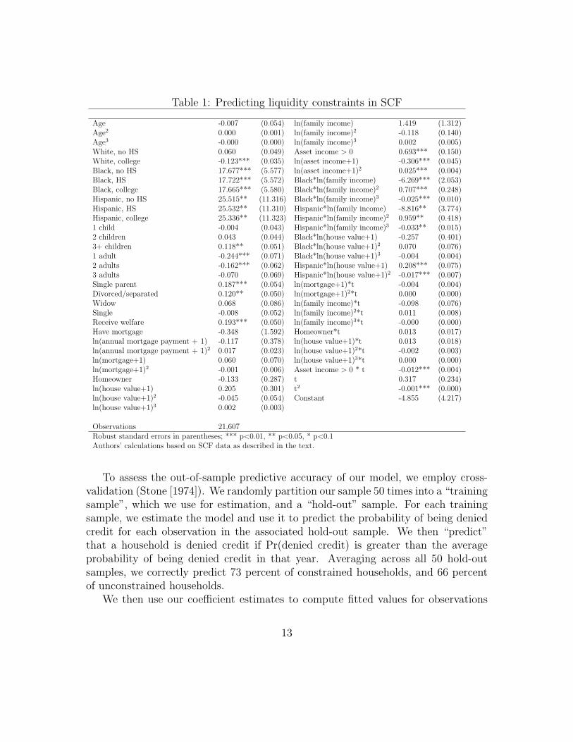
Table 1: Predicting liquidity constraints in SCF

Age -0.007 (0.054) ln(family income) 1.419 (1.312)Age2 0.000 (0.001) ln(family income)2 -0.118 (0.140)Age3 -0.000 (0.000) ln(family income)3 0.002 (0.005)White, no HS 0.060 (0.049) Asset income > 0 0.693*** (0.150)White, college -0.123*** (0.035) ln(asset income+1) -0.306*** (0.045)Black, no HS 17.677*** (5.577) ln(asset income+1)2 0.025*** (0.004)Black, HS 17.722*** (5.572) Black*ln(family income) -6.269*** (2.053)Black, college 17.665*** (5.580) Black*ln(family income)2 0.707*** (0.248)Hispanic, no HS 25.515** (11.316) Black*ln(family income)3 -0.025*** (0.010)Hispanic, HS 25.532** (11.310) Hispanic*ln(family income) -8.816** (3.774)Hispanic, college 25.336** (11.323) Hispanic*ln(family income)2 0.959** (0.418)1 child -0.004 (0.043) Hispanic*ln(family income)3 -0.033** (0.015)2 children 0.043 (0.044) Black*ln(house value+1) -0.257 (0.401)3+ children 0.118** (0.051) Black*ln(house value+1)2 0.070 (0.076)1 adult -0.244*** (0.071) Black*ln(house value+1)3 -0.004 (0.004)2 adults -0.162*** (0.062) Hispanic*ln(house value+1) 0.208*** (0.075)3 adults -0.070 (0.069) Hispanic*ln(house value+1)2 -0.017*** (0.007)Single parent 0.187*** (0.054) ln(mortgage+1)*t -0.004 (0.004)Divorced/separated 0.120** (0.050) ln(mortgage+1)2*t 0.000 (0.000)Widow 0.068 (0.086) ln(family income)*t -0.098 (0.076)Single -0.008 (0.052) ln(family income)2*t 0.011 (0.008)Receive welfare 0.193*** (0.050) ln(family income)3*t -0.000 (0.000)Have mortgage -0.348 (1.592) Homeowner*t 0.013 (0.017)ln(annual mortgage payment + 1) -0.117 (0.378) ln(house value+1)*t 0.013 (0.018)ln(annual mortgage payment + 1)2 0.017 (0.023) ln(house value+1)2*t -0.002 (0.003)ln(mortgage+1) 0.060 (0.070) ln(house value+1)3*t 0.000 (0.000)ln(mortgage+1)2 -0.001 (0.006) Asset income > 0 * t -0.012*** (0.004)Homeowner -0.133 (0.287) t 0.317 (0.234)ln(house value+1) 0.205 (0.301) t2 -0.001*** (0.000)ln(house value+1)2 -0.045 (0.054) Constant -4.855 (4.217)ln(house value+1)3 0.002 (0.003)

Observations 21,607Robust standard errors in parentheses; *** p<0.01, ** p<0.05, * p<0.1Authors’ calculations based on SCF data as described in the text.

To assess the out-of-sample predictive accuracy of our model, we employ cross-validation (Stone [1974]). We randomly partition our sample 50 times into a “trainingsample”, which we use for estimation, and a “hold-out” sample. For each trainingsample, we estimate the model and use it to predict the probability of being deniedcredit for each observation in the associated hold-out sample. We then “predict”that a household is denied credit if Pr(denied credit) is greater than the averageprobability of being denied credit in that year. Averaging across all 50 hold-outsamples, we correctly predict 73 percent of constrained households, and 66 percentof unconstrained households.

We then use our coefficient estimates to compute fitted values for observations

13

in the PSID sample, and interpret these fitted values as the probability that PSIDhouseholds are liquidity constrained. Starting in 1992, relative to SCF households,PSID households are about 2 percentage points less likely to be constrained, mostlikely because our SCF households include more welfare recipients and householdsheaded by Black and Hispanic individuals, and have lower average income. As longas the relationship between the probability of being constrained and the explanatoryvariables is the same in both samples, these differences should not matter.

We use the predicted probability of being constrained to proxy for the normalisedLagrange multiplier ln(1+λh,t−2) in the household’s Euler equation. We assume that

ln(1 + λh,t−2) = φ(Pr( denied credit)h,t−2) + uh,t−2 (9)

where φ is a polynomial function whose coefficients we estimate, Pr( denied credit)h,t−2

is the predicted probability that the household is liquidity constrained, and uh,t−2 isorthogonal to our instrument set.

1.2 Precautionary Savings

The variance of the household’s expectational errors, σ2h,t−2, appears in the Euler

equation because of the precautionary savings motive (Carroll [1992]). Precautionarysavings will be higher for households who are more uncertain about future income,and for households with lower wealth (Browning and Lusardi [1996]). We thereforeassume that the variance of household expectational errors can be approximated asa linear function of the variance of income volatility and the probability that thehousehold has positive wealth:

σ2h,t−2 = γh + γ1Et−2[(σ

Yh,t)

2] + γ2Pr(Wh,t > 0) + eσh,t−2 (10)

We allow the constant term γh to vary across households, since some households facesystematically higher uncertainty, regardless of their income volatility and wealth.In some specifications, we restrict γ2 to be zero. We assume the approximation erroreσh,t−2 is orthogonal to our instruments set.

1.2.1 Estimating Volatility of Family Income

To construct our measure of family income volatility, we estimate a standard modelof the household income process, and measure volatility as the square of changes inresiduals. Our model is:

ln(Yh,t) = X ′h,tϑt + uh,t (11)

14

Yh,t is real family income, and Xh,t is a set of household characteristics affect-ing income, which are observable, anticipated by consumers, and potentially time-varying.18 Standard models of the income process (MaCurdy [1982]) assume thatthe residual uh,t can be decomposed into a permanent and a transitory component;19

we do not make any particular assumption about uh,t, and do not attempt to distin-guish between permanent and transitory shocks in our main specification.We defineincome volatility, σ2

∆u,t, to be the variance of (uh,t − uh,t−2).Income is measured with error, and this measurement error appears to be non-

classical. While the textbook errors-in-variables model assumes that measurementerror is independent of true values, Kim and Solon [2005] find that measurementerror in survey data on earnings is mean-reverting and is negatively correlated withtrue values. Following Kim and Solon [2005], we assume observed household incomelnY ∗

h,t is a function of true income lnYh,t:

lnY ∗h,t = αh + λ lnYh,t + ϕh,t (12)

where αh is a household-specific fixed effect for reporting error, ϕh,t is white noisewith variance σ2

m, and 0 < λ < 1. Substituting this into our model of the incomeprocess, observed family income is:

ln(Y ∗h,t) = αh +X ′

h,tϑtλ+ uh,tλ+ ϕh,t (13)

Squared residuals from this equation will be consistent estimates of λ2σ2∆u,t+σ2

m,

rather than σ2∆u,t. We compute income volatility as

(∆uh,t)2

λ2, where λ = 0.67 as

estimated by Bound et al. [1994]. Notice that dividing observed income volatility by0.672 more than doubles the level of volatility and its change over time. The presenceof σ2

m biases our estimate of the level of income volatility, but as long as this variancedoes not vary over time, it does not bias our estimate of the trend.20

Figure 2 illustrates average household income volatility over the period 1980-2004 in deviations from its 1980 mean and after the effect of change in the surveymethodology (the effect of dummy for year > 1992) is corrected for, and its linear

18See Appendix A.3 for details.19A recent literature, following Guvenen [2007], has examined models with more heterogeneous

life-cycle income profiles and less persistent income shocks.20Since in 1993, the PSID converted the questionnaire to electronic form. Kim and Stafford [2000]

describe the changes PSID underwent. We therefore allow σ2m to be different before and after the

change in the survey. We remove the change in the variance of measurement error, by regressingincome volatility on a time trend and a dummy for year > 1992, and subtracting out the effect ofthe dummy.

15

−.0

50

.05

.1.1

5.2

mea

n v

olat

ility

1980 1985 1990 1995 2000 2005year

income volatility Fitted values

Figure 2: Mean Volatility of Household Income Shocks: deviations from 1980 mean.

Note: as (∆uh,t)2/λ2, where u2h,t is the squared residual from the family income regression (13)

and λ2 = 0.672 is the mean reversion correction as described in the text. Volatility is presented indeviations from the 1980 mean to correct for the presence of the measurement error, σ2

m, and afterthe effect of year > 1992 dummy is taken out, to correct for the change in the PSID surveymethodology.Source: Panel Study of Income Dynamics.

trend. Volatility of family income increased significantly between 1980 and 2004for an average household. This finding is consistent with the most recent study byDeBacker et al. [2013], who use a confidential panel of tax returns from the IRSto show that family income volatility increased between 1987 and 2009, as well asearlier studies (Dynan et al. [2012], Keys [2008], Gottschalk and Moffitt [2009], andGorbachev [2011]), based on PSID data, who find that household income volatilityincreased between 1970 and 2006.

1.2.2 Net Wealth

To measure cash on hand, we use information on households’ non-housing wealth.Information on wealth holdings in PSID is available for 1984, 1989, 1994, 1999, andbiennially thereafter. To fill in for the missing years and to reduce mis-measurement,we estimate the probability that the household had positive net non-housing wealth,

16

Pr(Wh,t > 0), based on other variables available in all years.21 We then predict theprobability of having positive non-housing net wealth for this and 4 previous years,

and use these predicted values as our proxy for cash on hand, Pr(Wh,t > 0).

2 Estimating Consumption Volatility

We are now ready to estimate our Euler equation 7. Due to presence of second andhigher order terms in the residual, it is typical to estimate the Euler equation usinginstrumental variable techniques or GMM. By rational expectations, any variablesknown at time t−2 will be orthogonal to the expectational errors. However, since thesecond-differenced preference shocks may not be orthogonal to time t− 2 variables,we use time t− s variables as instruments, where s ≥ 4.

If Xh,t−s is our set of instruments, then our identifying assumptions are

E

[

ςh,t

∣

∣

∣Xh,t−s

]

= 0 (14)

E

[

ln(1 + λh,t−2)− φ(Pr( denied credit)h,t−2)|Xh,t−s

]

= 0 (15)

E

[

σ2h,t−2 − γh − γ1(σ

Yh,t)

2 − γ2Pr(Wh,t > 0)|Xh,t−s

]

= 0 (16)

Restrictions (15) and (16) are necessary because we use proxy variables to esti-mate the effects of ln(1 + λh,t−2) and σ2

h,t−2, which are unobserved, on the growthrate of consumption. Using proxy variables introduces approximation errors. Theconsistency of our estimates requires that the instruments we choose are orthogonalto these approximation errors. In practice, we may under predict or over predict theLagrange multiplier or σ2

h,t−2; what is crucial is that this error is not correlated withthe characteristics of the household s years ago.

Combining household fixed effects into a single term, κh =β

γ(γh− 2δh−Rh), the

21See Appendix A.3 for details.

17

equation we estimate is:

∆ lnFh,t =κh +β

γln(1 + rh,t) + α1∆ ln pFt + α2∆ ln pOt (17)

+β

γ

[

ηW∆NWh,t + ηH∆NH

h,t

]

+ µ∆Zh,t

+β

γ

[

φ(Pr( denied credit)h,t−2) + γ1(σYh,t)

2 + γ2Pr(Wh,t > 0)]

+ ςh,t (18)

The standard fixed effects estimator is inconsistent in a dynamic panel data model(Nickell [1981]). We therefore estimate (17) using the Arellano and Bover [1995]two-step GMM estimator, which uses forward orthogonal transformations to removethe fixed effects. The forward orthogonal transformation subtracts the average of allfuture available observations of a variable, thus preserving the length of the sample.22

The observable variables affecting preferences, ∆Zh,t, include age, age squared,change in number of adults, change in number of children, change in marital status,and an indicator variable for change in home ownership.23 After testing for autocor-relation in the residuals we find that it is present up to the third lag. We thereforeuse variables dated t − 4 and t − 5 as instruments. We limit the number of instru-ments to two lags and “collapse” our instruments to a single column to reduce theefficiency loss caused by too many instruments.24 We allow for heteroskedasticity andintra-group correlation, and make the Windmeijer [2005] finite-sample correction toour standard errors.

Table 2 reports our estimation results. In column (1), we report results from ourbasic specification of the Euler equation in which we assume separable preferencesbetween food, other non-durables, labour supply and housing. In Columns (2) to(4), we progressively relax these assumptions. Column (2) allows for non-separablepreferences for food, other non-durables and labour supply, by including prices andthe change in hours worked by both the spouse and head of the household.25 In

22If wh,t is a variable, its forward orthogonal transform is

√

Th,tTh,t+1

(wh,t −1

Th,t

∑

s>t wh,s).

23This variable equals 1 when the household goes from renting to owning, equals 2 when thehousehold moves from public housing to owning, is negative if the direction is reversed, and equalszero when there is no change.

24Roodman [2009] describes the problems too many instruments could cause this type of GMMestimator.

25As discussed above, while hours worked are endogenous - in particular, because householdmembers adjust labor supply to insure against shocks (Blundell et al. [2012]) - we deal with thisendogeneity problem by using variables known at date t−4 or earlier as instruments. Our identifying

18

Table 2: Euler Equation Estimation, biennial sample, 1980 to 2004.(1) (2) (3) (4)

ln(1 + rh,t) 0.570** 0.609** 0.704** 0.513*(0.266) (0.257) (0.289) (0.293)

(σYh,t)

2 0.054 0.039 0.093 0.069(0.076) (0.051) (0.062) (0.063)

Pr( denied credit) 2.389 2.145* 2.741* 1.467(1.769) (1.277) (1.642) (1.597)

Pr( denied credit)2 -9.671* -8.282* -12.654* -7.708(5.825) (4.774) (7.077) (6.749)

Pr( denied credit)3 10.818* 9.243* 14.837* 9.938(6.367) (5.473) (8.045) (7.706)

∆ ln pO 0.266 0.208 0.397*(0.197) (0.211) (0.236)

∆ ln pF -0.334 -0.244 -0.890(0.458) (0.484) (0.640)

Age -0.008 -0.008 -0.007 -0.010(0.009) (0.006) (0.007) (0.013)

Age2 0.000 0.000 0.000 0.000(0.000) (0.000) (0.000) (0.000)

Change in number of adults 0.127** 0.104** 0.065 0.114*(0.055) (0.051) (0.064) (0.066)

Change in number of kids 0.052 0.066 0.108** 0.097(0.049) (0.044) (0.046) (0.065)

Change in marital status 0.059 0.045 0.160 0.048(0.178) (0.135) (0.162) (0.152)

Change in house ownership -0.007 -0.001(0.101) (0.109)

Change in number of hours worked, spouse 0.015* 0.018** 0.016(0.008) (0.009) (0.010)

Change in number of hours worked, head -0.008 -0.025 0.023(0.045) (0.047) (0.050)

Pr(Wh > 0) 0.221(0.284)

Number of observations 34,002 34,002 34,002 30,524Number of households 5,514 5,514 5,514 5,102Number of Instruments 24 36 30 32F-stat 32.13 30.14 25.31 20.72Prob>F 0 0 0 0Sargan test of overid 16.12 21.20 18.13 15.56df 14 22 15 16Prob> χ2 0.306 0.710 0.478 0.484Hansen test of overid 13.06 17.93 14.63 13.49df 14 22 15 16Prob> χ2 0.522 0.508 0.256 0.637Robust standard errors in parentheses; *** p<0.01, ** p<0.05, * p<0.1

Note: we instrument: ln(1 + rh,t), Pr( denied credit) and its polynomial, Pr(Wh > 0) ,(σY

h )2, ∆ ln pO, ∆ ln pF , change in the number of adults, change in the number of kids,

change in marital status, change in the number of hours worked by head and spouse,with t− 4 and t− 5 lags of these variables, time dummies, and marginal tax rates.Authors’ calculations based on PSID and SCF data as described in the text.

19

column (3), we also allow for non-separable preferences over housing by includingthe indicator variable for change in homeownership. In column (4) we add theprobability that the household has positive wealth as a proxy for cash on hand inthe precautionary savings term.

We report the results of the Hansen and Sargan tests for overidentifying restric-tions. Unlike the Sargan test, the Hansen J test is robust to non-spherical errors butcan be weakened by too many instruments. In all cases, we fail to reject the hypoth-esis that the overidentifying restrictions are valid. In addition, our set of explanatoryvariables is highly statistically significant in all specifications, according to the jointsignificance test.

In all specifications the coefficient on the interest rate is statistically significantat the 5 percent level. If we assume preferences over food are homothetic (β = 1), weestimate the intertemporal elasticity of substitution, 1

γ, to be between 0.57 and 0.7.

If we allow preferences to be non-homothetic (β 6= 1), because we believe that food isa necessity, then this coefficient cannot be interpreted as the intertemporal elasticityof substitution; rather, it equals the IES multiplied by the budget elasticity of foodconsumption with respect to total non-durable expenditure, β. Using Consumer Ex-penditure Survey data for 1980-1992 period, Blundell et al. [2008] estimated β = 0.85,and found that the budget elasticity fell during that time period. We re-estimateBlundell et al. [2008]-type regressions on PSID data using the newly available infor-mation on non-durable expenditure for 2005-2009 data. We find β = 0.78.26 Usingthis estimate, our results imply an IES of between 0.73 and 0.9, which is in line withevidence from other studies using microeconomic data (Attanasio [1999]).

Consumption growth should be larger for liquidity constrained households andhouseholds experiencing higher income volatility, who have a higher precautionary

saving motive. Our coefficients on the polynomial in Pr( denied credit) imply a non-monotonic relationship between the probability of being constrained and consump-tion growth. The effect of (σY

h )2 is always positive, though it is never statistically

assumption is that unexpected shocks to consumption growth are not correlated with predictablechanges in hours worked. This is true under our maintained assumption that households haverational expectations.

26In addition to expenditure on food at home and away from home, starting in 1999, the PSIDadded information on the following non-durable (and services) categories: childcare (for workingand non working spouses), utilities, gasoline, transportation, home and auto insurance, and vehiclerepair. Moreover, in 2005, additional categories for non-durable consumption were added. Theseinclude expenditure on clothing, home repair, furniture, trips, and other recreation activities. Wedefine non-durable consumption based on the information available starting 2005. We use dataon detailed consumption categories kindly provided to us by Geng Li of Federal Reserve Board.Details of our estimation are described in the Appendix, section A.4.

20

−.0

50

.05

.1.1

5.2

mea

n v

olat

ility

1980 1985 1990 1995 2000 2005year

income volatility consumption volatilityFitted values Fitted values

Figure 3: Mean income volatility and consumption volatility for 1980 to 2004

Note: Household income volatility is computed as (∆uh,t)2/λ2, where u2h,t is the squared residual

from the family income regression (13) and λ2 = 0.672 is the mean reversion correction asdescribed in the text. Consumption volatility is computed as (ςh,t − κh)

2, where ςh,t is theresidual and κh is the household fixed effect from the Euler equation (18). Volatility ofconsumption and of income are presented in deviations from their respective 1980 means tocorrect for the presence of measurement error, and after the effect of year> 1992 dummy wastaken out, to correct for the change in the PSID survey methodology.Source: Panel Study of Income Dynamics.

significant.

2.1 Evolution of Consumption Volatility

To compute volatility of household consumption, we first predict residuals, ςh,t, fromthe above Euler equation, using our preferred specification, that in column 3 of the

table 2. We then subtract out household fixed effects κh =β

γ(γh − 2δh − Rh), that

are not directly computed by the AB-GMM estimator. Our measure of consumptionvolatility is (ςh,t − κh)

2. Recall that our measure of consumption volatility containsother terms, such as variances of measurement error, second and higher order termsand second-differenced preference shocks, which we are not directly interested in

21

computing, but cannot estimate separately. Since our goal is to measure the changein consumption volatility over time, this is not a problem, assuming these other termsdo not vary over time.27

Figure 3 shows deviations from the 1980 mean for income and consumptionvolatilities between 1980 and 2004, and their respective linear trends. As in Fig-ure 2, the volatility series presented in deviations from their respective 1980 meansto correct for the presence of measurement error. The graph in the figure is also cor-rected for the change in the survey methodology. Consumption volatility increased3 volatility points, from an average of 14.6 in 1980-1984 to an average of 17.5 in2000-2004, or by 19 percent. However, income volatility rose by 44 percent, or by14 volatility points, over the same period. We should note that our estimate of thepercentage point change in income volatility is highly sensitive to the mean-reversioncorrection, λ2 = 0.672, though the estimate of the percentage change in volatility ofincome is not affected by this correction. However, since measurement error causes usto overestimate the level of consumption and income volatilities, it biases downwardsour estimates of their percentage change. Our estimate of a 19 percent increase involatility of food consumption is therefore a lower bound.

Figure 4 shows consumption and income volatility for particular demographicgroups. The levels of consumption and income volatility were around 7 and 10volatility points higher, respectively, for black or Hispanic households relative towhite households. Consistent with previous studies, income volatility was higherfor less educated than for more educated households, though the trends in incomevolatility for these two groups have been converging over the sample period. Con-sumption volatility disaggregated by education, exhibited similar trends to those ofincome volatility, though the differences were not as pronounced.

To test whether the increase in volatility and the differences in the levels ofvolatility across households are statistically significant, we regress our squared Eulerequation residuals on a time trend, change in survey methodology correction term

27To allow for the possibility that the variance of measurement error in consumption also changedfollowing the move to electronic surveys in 1992, we regress consumption volatility on a time trendand a dummy for year > 1992, and subtract the effect of the dummy from our estimate, followingthe strategy we used for correcting volatility of income, described earlier.Moreover, our Euler residuals also contain the error ut, the difference between the Lagrange

multiplier and the polynomial in the predicted probability of being denied credit, equation (9). Inprinciple, the variance of ut could trend over time, if for example, our probit estimates becomemore or less accurate over time, biasing our estimates of the trend in consumption volatility. Inpractice, the variance of our probit errors (within the SCF sample) has only a moderate trendover time, increasing from 0.13 in 1983 to 0.14 in 2007. If we attempt to purge our consumptionvolatility estimates of these errors, the trend in volatility remains positive, significant, and of thesame magnitude (results are available upon request).

22

.3.4

.5.6

.7m

ean

vola

tility

1980 1985 1990 1995 2000 2005year

White Black\Hispanic

Fitted values Fitted values

.3.4

.5.6

.7m

ean

vola

tility

1980 1985 1990 1995 2000 2005year

Edu<13 Edu>12

Fitted values Fitted values

Income Volatility.1

.15

.2.2

5.3

mea

n vo

latil

ity

1980 1985 1990 1995 2000 2005year

White Black\Hispanic

Fitted values Fitted values

.1.1

5.2

.25

.3m

ean

vola

tility

1980 1985 1990 1995 2000 2005year

Edu<13 Edu>12

Fitted values Fitted values

Consumption Volatility

Figure 4: Mean income volatility and consumption volatility for 1980 to 2004

Note: Household income volatility is computed as (∆uh,t)2/λ2, where u2h,t is the squared residual

from the family income regression (13) and λ2 = 0.672 is the mean reversion correction asdescribed in the text. Consumption volatility is computed as (ςh,t − κh)

2, where ςh,t is theresidual and κh is the household fixed effect from the Euler equation (18).Source: Panel Study of Income Dynamics.

(year> 1992 dummy), and demographic controls. For comparison, we run the sameregressions using income volatility. Table 3 reports these results. Columns (1) and(2) provide results from a regression on a linear time trend. Volatility of consumptionincreased by 1.5 points every 10 years, or by 3.5 points between 1980 and 2004. Incontrast, volatility of income rose by 7 points every 10 years, or 17 percentage pointsbetween 1980 and 2004. Both trends are statistically significant at the 1 percentlevel. In columns (3) and (4) we allow for differential levels in volatility by race

23

Table 3: Evolution of Food Consumption and Income Volatility, biennial sample, 1980 to 2004.(1) (2) (3) (4) (5) (6)food income food income food income

Year/1000 1.464*** 6.971*** 1.585*** 7.419*** 1.652*** 8.510***(0.509) (1.490) (0.507) (1.494) (0.566) (1.742)

Year > 1992 -0.007 0.060*** -0.006 0.063*** -0.006 0.063***(0.007) (0.022) (0.007) (0.022) (0.007) (0.022)

Black/Hispanic 0.067*** 0.095*** -2.276 -4.030(0.010) (0.027) (2.206) (6.038)

Education< 13 0.015*** 0.046*** 0.814 5.773*(0.005) (0.016) (1.215) (3.488)

Black/Hispanic × year/1000 1.176 2.070(1.107) (3.035)

Education< 13 × year/1000 -0.401 -2.875(0.610) (1.753)

Age -0.004** -0.028*** -0.004* -0.028***(0.002) (0.006) (0.002) (0.006)

Age2 0.000* 0.000*** 0.000* 0.000***(0.000) (0.000) (0.000) (0.000)

Constant -2.755*** -13.507*** -2.921*** -13.840*** -3.054*** -16.015***(1.010) (2.958) (1.007) (2.958) (1.124) (3.456)

Number of observations 33,652 33,652 33,652 33,652 33,652 33,652Adj. R2 0.001 0.006 0.005 0.008 0.005 0.008Robust, clustered at household level, standard errors in parentheses;*** p<0.01, ** p<0.05, * p<0.1Note: in columns (3) to (6) other controls, not shown to conserve space, include change in maritalstatus, change in the number of kids and the number of adults.Source: Authors’ calculations based on PSID and SCF data as described in the text.

and education, and in columns (4) and (5) also for different trends, and a quadraticpolynomial in age. These results confirm that the differences between demographicgroups shown in Figure 4 are statistically significant: consumption volatility is 7points higher for Black and Hispanic households than for white households, and is 1.5points higher for households whose head had less than 13 years of education. UnlikeGorbachev [2011], we do not find a statistically significant difference in the trendsof income and consumption volatility for white and black or Hispanic households.We find support of previous findings that income volatility is u-shaped: it is high ata young age, falls during the mid-years, and rises again later in life. Consumptionvolatility follows a similar pattern. Nevertheless, controlling for age does not reducethe magnitude of the increase in income or consumption volatility, indicating thatthe increase in volatility is not explained by the ageing of our sample or by its life-cycle properties. In regressions not shown, but available in the Appendix, TableA.4, we also control for changes in marital status, and changes in the number ofadults and children in the household. We find that marital status changes have asignificant and positive impact on volatility of consumption and income (i.e. they

24

Table 4: Effect of Liquidity Constraints and Income Uncertainty on Volatility of Consumption,biennial sample, 1980 to 2004.

(1) (2) (3) (4) (5) (6)OLS OLS OLS OLS IV IV

Year/1000 1.145** 0.532 0.323 0.266 0.259 0.159(0.496) (0.512) (0.504) (0.501) (0.498) (0.507)

Year > 1992 -0.010 -0.007 -0.010 -0.010 -0.011 -0.011(0.007) (0.007) (0.007) (0.007) (0.007) (0.007)

(σYh,t)

2 0.052*** 0.050*** 0.062*** 0.071*** 0.088***(0.004) (0.004) (0.008) (0.009) (0.019)

Pr( denied credith,t−2) 0.221*** 0.186*** 0.216*** 0.167*** 0.220***(0.024) (0.024) (0.025) (0.050) (0.066)

Pr( denied credith,t−2)× (σYh,t)

2 -0.051** -0.081(0.024) (0.077)

Black/Hispanic 0.061*** 0.024** 0.026** 0.025** 0.028** 0.025**(0.010) (0.011) (0.011) (0.011) (0.012) (0.012)

Education< 13 0.012** -0.000 -0.000 -0.000 0.000 -0.000(0.005) (0.005) (0.005) (0.005) (0.005) (0.005)

Age -0.002 0.000 0.001*** 0.001*** 0.001** 0.001***(0.002) (0.002) (0.000) (0.000) (0.000) (0.000)

Change in Marital Status 0.092*** 0.096*** 0.085*** 0.085*** 0.081*** 0.080***(0.011) (0.012) (0.011) (0.011) (0.011) (0.011)

Constant -2.119** -0.987 -0.595 -0.488 -0.279 -1.310(0.985) (1.015) (0.999) (0.994) (0.999) (2.613)

Number of Observations 33,652 33,652 33,652 33,652 33,652 33,652Adj. R2 0.036 0.015 0.040 0.040 0.035 0.036Number of excluded instruments 3 3Kleibergen-Paap rk LM statistic 135.4 69.97Prob > χ2 0 0weak id Kleibergen-Paap rk Wald F statistic 167.7 29.38Hansen J statistic 1.147 -p-value 0.284 -Robust, clustered at household level, standard errors in parentheses;*** p<0.01, ** p<0.05, * p<0.1

Note: Columns (5) and (6) instrument Pr( denied credit) and (σYh,t)

2 with cohort-year-industry averages

of (σYh,t)

2, and Pr( denied credit) with cohort-year-state averages of Pr( denied credit), and their interaction,with the interacted instruments.Source: Authors’ calculations based on PSID and SCF data as described in the text.

increase volatility). However, changes in the size of the household appear to beunimportant. In addition, inclusion of cohort and state fixed effects, to account forcompositional changes and for differential levels of volatility that are cohort and/orgeography specific, do not change our main results.

Next we investigate the relation between liquidity constraints, income volatility

25

and consumption volatility. Table 4 presents these results. Columns (1) and (2)illustrate the individual effects of income volatility or liquidity constraints, respec-tively, on volatility of consumption; column (3) includes both variables, and column(4) adds an interaction between them. Each of these variables, volatility of incomeand our proxy for liquidity constraints, has a positive and significant effect on con-sumption volatility. The interaction term has a negative sign; this is surprising,since in theory income shocks should have a larger effect on consumption volatilityfor liquidity constrained households. This appears to be driven by a nonlinear rela-tion between income volatility and consumption volatility when income volatility isextremely high.28 We find that the trend in consumption volatility is completely ex-plained by the trend in liquidity constraints, either alone or together with the trendin income volatility. A household which is 10 percentage points more likely to beliquidity constrained has, on average, between 1.9 and 2.2 points higher consump-tion volatility. Reducing volatility of income by 10 points would reduce volatility ofconsumption by between 0.5 and 0.6 points. These results remain unchanged withthe inclusion of state and cohort fixed effects.

To deal with potential mis-measurement of true liquidity constraints and incomeuncertainty, we instrument for income volatility and the probability of being deniedcredit. Columns (5) and (6) report these results. To instrument for income volatilitywe construct industry-time-cohort specific averages of income volatility. Althoughthe choice of industry in itself is endogenous, the level of volatility for a specificyear-cohort pair within an industry will be a good indicator of the level of volatilityexperienced by individuals working in that sector, and will be subject to less variationthan an individual specific measure, alleviating the problem of mis-measurement. Toinstrument for liquidity constraints, we construct state-time-cohort averages of theprobability of being denied credit. This instrument will pick up state level lendingdifferences as well as differences within state and over time for a specific cohort ofindividuals. We interact these averaged effects to instrument for the interaction ofliquidity constraint and income volatility term. In column (5) we drop the interac-tion term and use all three instruments, and in column (6) we also instrument theinteraction term. In both cases, the effect of income volatility and the probability of

28Income volatility occasionally takes extremely large values, whereas this is not true for con-sumption volatility. Thus when income volatility is high, consumption volatility is likely to be aconcave function of income volatility, even if there is generally a linear relation between the twovariables. Since income volatility and liquidity constraints are correlated, the negative interactionterm may, in part, be proxying for a nonlinear relation between income and consumption volatility.Consistent with this observation, we find that if we omit observations with income volatility in thetop 1 percent of the income volatility distribution, the interaction term falls to zero, while the othercoefficients remain similar. These results are available upon request.

26

being denied credit remains positive, and of a similar size as in our OLS specifica-tion (columns (3) and (4)), although the effect of income volatility is slightly larger.When instrumenting, we loose the significance of the interaction term. In both spec-ifications, the tests of the validity of our instruments are passed with high statisticalsignificance. Moreover, our instruments do not suffer from the problems caused byweak identification, as the F-statistics are large for both regressions, especially forthe overidentified case in column (5).

Households with higher transitory income volatility will find it harder to smoothconsumption, and will be more likely to be denied credit. Thus although householdswho are more likely to be denied credit have higher consumption volatility, thismight not be because they have less access to credit; instead, it might be becausethese households might have higher transitory income volatility. It is hard to addressthis concern directly: since the SCF has essentially no panel dimension, we cannotseparately estimate temporary and permanent income shocks. One approach is tosplit our sample by education. It is well known that individuals with less educa-tion face more volatile transitory income shocks, and less volatile permanent shocks(Gundersen and Ziliak [2008]). If we find that splitting the sample by education re-duces the effect of liquidity constraints on consumption volatility, that would suggestthat what we call an “access to credit” affect merely reflects differences in transitoryvolatility. We do not find this to be true.29 The effect of liquidity constraints islarger for the less educated than for the better educated group, 0.24 vs. 0.18, butthis difference is statistically insignificant; more importantly, the average effect ofliquidity constraints is similar to the effect in our whole sample. This suggests thatthe endogeneity problem described here is not of great concern in practice.

Our results indicate that if we took an average household in the 25th percentile

of the Pr( denied credit) distribution, with a 9 percent probability of being liquidityconstrained, and moved this household to the 75th percentile with a 31 percent prob-ability of being constrained, while holding the size of their income shock constant,we would raise their consumption volatility by 5 points, or around 40 percent. Notethat when we control for both volatility of income and probability of being deniedcredit, the time trend becomes insignificant. This suggests that if these key variablesremained unchanged during this period, volatility of consumption would have alsoremained constant. In all specifications, our main conclusion remained unchanged:liquidity constraints play a crucial role in propagating income shocks.

These results are important given the substantial inequality in households’ accessto credit. In our SCF sample, around 40 percent of households with a black orHispanic head of household were liquidity constrained, compared to 20 percent of

29These results are available in Appendix Table A.5.

27

households headed by a white individual; around 30 percent of households whosehead had less than 13 years of education were constrained, compared to 20 percentof households with at least 13 years of education. There is no evidence that thesegroups are more likely to apply for loans. In fact, according to SCF data, blackindividuals and less educated individuals were less likely to apply for loans thanwhite or highly educated individuals between 1995 and 2007 (although they weresignificantly more likely to be discouraged from applying because they thought theywould be denied). It remains unclear whether lenders are less willing to extendcredit to these households because they have more volatile incomes and a higher riskof default, or because of other reasons, such as discrimination.

Wealth inequality can also explain differences in consumption volatility betweenhouseholds. According to SCF data, asset poverty (defined as households with netassets less than two months’ income) among blacks and Hispanics fell by a quarterbetween 1983 and 2007, nevertheless, blacks and Hispanics remain twice as likelyto be asset poor as whites. College educated households are significantly less likelyto be asset poor. Although we do not attempt to identify the causal affect of assetpoverty on consumption volatility, it seems likely that wealth inequality, in additionto inequalities in access to credit markets, contributed to disparities in households’ability to smooth consumption.30

3 Conclusion

The volatility of US household income increased by 44 percent between 1980 and2004. Households were not able to completely smooth consumption in response totheir increasingly volatile income shocks: over the same period, the volatility of un-predictable changes in household consumption increased by around 19 percent. Onefactor limiting households’ ability to smooth was limited access to credit. Between1983 and 2007, around 1 in 5 households were denied a loan or were discouraged fromapplying for a loan in the past 5 years, and the proportion of liquidity constrainedhouseholds increased slightly over time. While financial sector innovations such ascredit scoring and risk-based pricing may have increased lenders’ willingness to lend,it seems that households’ demand for credit has increased by the same amount, sothat the fraction of households unable to borrow as much as they would like re-

30Another partial insurance mechanism, which we do not explore in this paper, is risk-sharingwithin family networks. Our measure of income volatility is post-transfers (both private and public)but pre-tax. Thus, the income volatility process is smoother than it would have been if transferswere excluded. A proper investigation into the effect of household risk sharing on consumptionvolatility is left for future research.

28

mained unchanged. Differences in households’ net wealth and access to credit led tosignificant differences in their ability to smooth consumption.

The increase in the volatility of household consumption has a significant welfarecost. Accurately estimating this welfare cost is beyond the scope of this paper. Toshow that the welfare cost is likely to be substantial, we use Lucas [1987]’s formula forthe cost of consumption fluctuations to obtain a rough estimate. Lucas [1987] consid-ered a representative consumer with isoelastic, time separable utility, and assumedthat log consumption is normally distributed with variance σ2

c around a linear trend.Under these assumptions, eliminating all consumption volatility would provide thesame welfare benefit as increasing annual consumption by µ = 1

2γσ2

c percent. UnlikeLucas, we are considering the variance of unpredictable changes in household con-sumption, not the variance of deviations of aggregate consumption from a trend.31

Since the elasticity of food consumption with respect to total non-durable consump-tion is β, shocks to food consumption growth will be β times as large as shocks to totalconsumption growth, and the variance of shocks to food consumption growth (ourmeasure of consumption volatility) will be β2 times as large as the variance of shocksto total consumption growth. We therefore divide our measure of food consumptionvolatility by β2, using our estimate of β = 0.78. In our Euler equations, we estimateβ/γ = 0.6; we therefore take γ = 0.78/0.6 = 1.3. Under these assumptions, reducingconsumption volatility by 2.8 points from its 2000-2004 level to its 1980-1984 levelwould produce the same welfare gain as increasing annual non-durable consumptionby 3 percent.32 While this number is only a back of the envelope estimate, and issensitive to assumptions, it is clear that the rise in consumption volatility is of firstorder importance for household welfare.

Similarly, since disadvantaged groups face higher levels of consumption volatil-ity, driven in part by differences in access to credit, decreasing their consumptionvolatility would have a clear welfare benefit. Households headed by a black or His-panic individual have on average 7 points higher consumption volatility than whites.Reducing consumption volatility for the average black or Hispanic household to thelevel experienced by the average white household would provide the same welfare

31In our model consumption is close to a random walk with drift, rather than trend-stationary.Reis [2009] shows that this change in assumptions can increase the welfare cost of fluctuations byan order of 50. Our welfare cost estimate should therefore be considered a lower bound. Our resultsare of the same order of magnitude as Hai et al. [2013], who calculate the welfare cost of fluctuationsin a structural model with memorable goods, fitted to CEX data.

32We compute welfare cost as 1

2γ(σ2

c,2000−2004−σ2c,1980−1984) =

1

2γ(σ2

f,2000−2004− σ2

f,1980−1984)

β2=

1

2∗ 1.3 ∗

0.028

0.782= 0.03.

29

gain as increasing annual consumption by around 7.3 percent. The difference be-tween consumption volatility for the quarter of households most likely to be liquidityconstrained and the quarter of households least likely to be constrained is of the samemagnitude. This suggests that improving access to credit for disadvantaged groups,or providing them with other ways to smooth consumption, could significantly im-prove household welfare.

30

A Web Appendix

A.1 Data Sample: Panel Study of Income Dynamics

The Panel Study of Income Dynamics (PSID), which began in 1968, is a longitudinalstudy of a representative sample of U.S. individuals (men, women, and children) andthe family units in which they reside, and is conducted by the University of Michigan.The PSID’s sample size has grown from 4,800 families in 1968 to more than 7,000families (and over 60,000 individuals) in 2001. Some families are followed for as muchas 36 consecutive years.

Consumption data in PSID are limited to food and shelter. We compute all theconsumption volatility measures on food consumption calculated as a sum of foodconsumed at home plus away from home plus food stamps received. The core samplecontains data from 1968 to 2005, and consists of heads of households (both femaleand male) who are not students and are not retired. We keep households whose headis at least 25 years old but less than 65. We drop all the households that belongedto the Latino or Immigrant samples, and those that were drawn from the Survey ofEconomic Opportunity (SEO). Households that report negative or zero total foodconsumption levels are also eliminated. In order to minimise effects of outliers on theresults, we follow the literature by dropping households who report more than 500percent change in family income or food consumption over a one year period as wellas those whose income or consumption fall by more than 95 percent (see for exampleZeldes [1989b] or Blundell et al. [2008]).

The most important issue to note regarding the data is that it became biennialafter 1997. We construct a hypothetical biennial sample to study the evolution ofconsumption volatility up to 2004. Since income and consumption data is collectedfor the previous year, the biennial sample has data for even years from 1976 to2004. In addition, food consumption data was not collected in 1973, 1988 and 1989.We do not impute for the missing years in order to keep measurement error andmisidentification to a minimum.

At the time of the interview, the respondent is asked questions about income,transfers, wealth and expenditures on food and shelter. The families are asked toreport income and transfers received during the previous year. We use total familyincome to compute income uncertainty. We adjust income data by one period tocorrespond to the appropriate demographic characteristics for each household. Thetiming of consumption data is more ambiguous. We follow Blundell et al. [2008],among many others, and assume that the respondent provided information on foodexpenditures for the previous year. We use interest rates on two-year constant ma-

31

turity Treasury bills.All the income, expenditure, wealth, and interest rate data are expressed in real

terms. Nominal data are converted into real using item specific regional not season-ally adjusted all urban Consumers Consumer Price Index (CPI-U) with base periodof 1982-1984=100. Thus, food expenditures are deflated using the Food and Bever-ages CPI; housing expenditures, using the Housing CPI; and all income, wealth andinterest rate series, using All-Items CPI.

A.2 Data Sample: Survey of Consumer Finances

The 1983, 1989, 1992, 1995, 1998, 2001, 2004 and 2007 Surveys of Consumer Finances(SCF), sponsored by the Board of Governors of the Federal Reserve System, arecross-sectional surveys of the balance sheet, pension, income, and other demographiccharacteristics of U.S. families. The SCF collects data from two samples: a standardmulti-stage area-probability sample selected from the 48 contiguous US states, anda list sample designed to disproportionately sample wealthy families. For example,3,007 of the 4,522 interviews for the 2004 SCF were from the area probability sample,and 1,515 were from the list sample, therefore the total sample is not representative ofUS households. The SCF provides probability weights which account for the sampledesign, and also for differential patterns of non-response among families with differentcharacteristics; unless otherwise noted, all SCF data presented here is weighted.

Over 1989-2007, the SCF uses a multiple imputation method to account for miss-ing data. For each piece of missing data, the SCF provides 5, possibly different,responses (referred to as “implicates”), resulting in a data set with 5 times theactual number of households. We average across all five implicates to reduce thelikelihood of biasing our results. Lindamood et al. [2007] report that using only oneimplicate may bias results; ideally, all implicates should be used according to the“repeated-imputation inference” method.

A.3 Variables Used in Regressions

In our probit regression model for the probability of being denied credit in SCFdata, our explanatory variables are: a cubic in age, categorical variables for a femalehead of household, a single parent, marital status, receiving welfare payments, havingpositive asset income; cubics in log income and house value, quadratic functions of logannual mortgage payments, mortgage, and asset income; and interactions betweenrace, education (no high school, high school, or college), and the cubic in log housevalue. We test for coefficient stability by interacting these variables with linear and

32

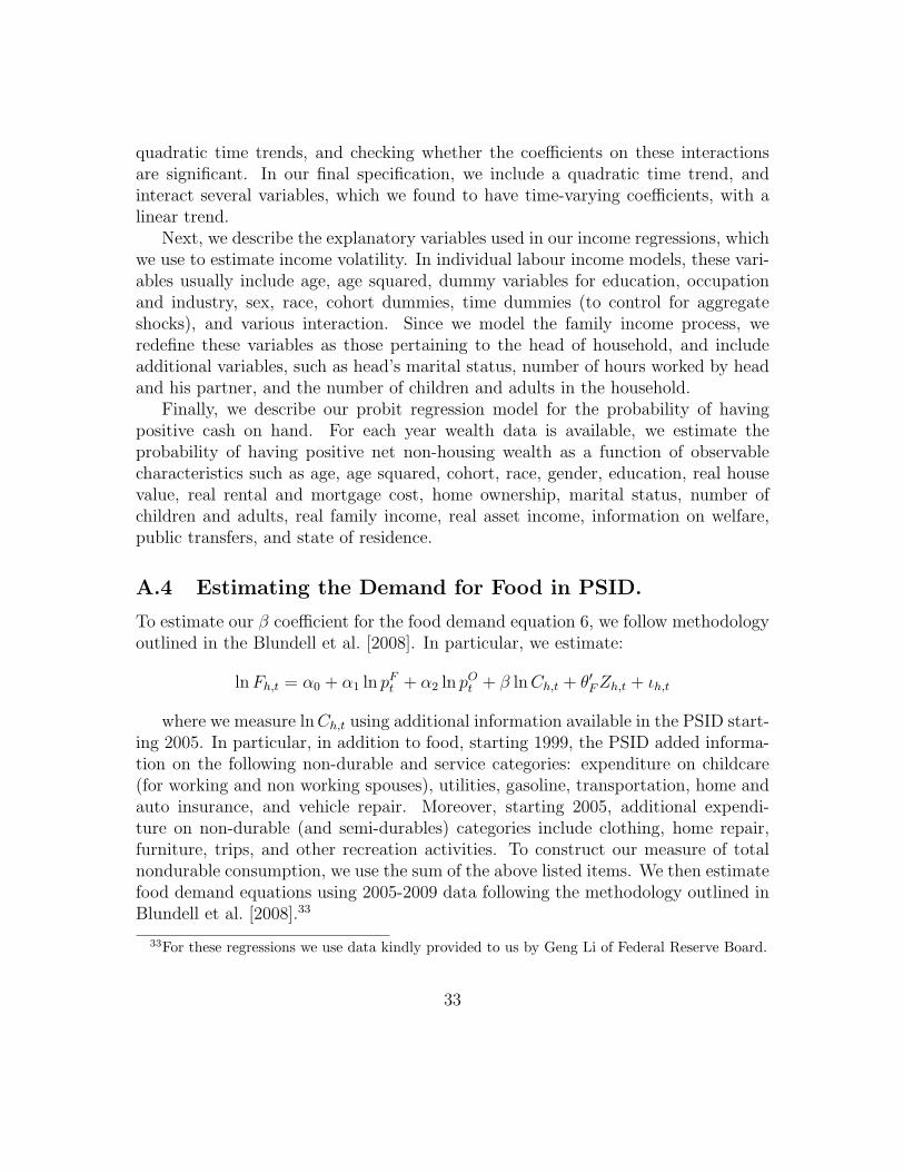
quadratic time trends, and checking whether the coefficients on these interactionsare significant. In our final specification, we include a quadratic time trend, andinteract several variables, which we found to have time-varying coefficients, with alinear trend.

Next, we describe the explanatory variables used in our income regressions, whichwe use to estimate income volatility. In individual labour income models, these vari-ables usually include age, age squared, dummy variables for education, occupationand industry, sex, race, cohort dummies, time dummies (to control for aggregateshocks), and various interaction. Since we model the family income process, weredefine these variables as those pertaining to the head of household, and includeadditional variables, such as head’s marital status, number of hours worked by headand his partner, and the number of children and adults in the household.

Finally, we describe our probit regression model for the probability of havingpositive cash on hand. For each year wealth data is available, we estimate theprobability of having positive net non-housing wealth as a function of observablecharacteristics such as age, age squared, cohort, race, gender, education, real housevalue, real rental and mortgage cost, home ownership, marital status, number ofchildren and adults, real family income, real asset income, information on welfare,public transfers, and state of residence.

A.4 Estimating the Demand for Food in PSID.

To estimate our β coefficient for the food demand equation 6, we follow methodologyoutlined in the Blundell et al. [2008]. In particular, we estimate:

lnFh,t = α0 + α1 ln pFt + α2 ln p

Ot + β lnCh,t + θ′FZh,t + ιh,t

where we measure lnCh,t using additional information available in the PSID start-ing 2005. In particular, in addition to food, starting 1999, the PSID added informa-tion on the following non-durable and service categories: expenditure on childcare(for working and non working spouses), utilities, gasoline, transportation, home andauto insurance, and vehicle repair. Moreover, starting 2005, additional expendi-ture on non-durable (and semi-durables) categories include clothing, home repair,furniture, trips, and other recreation activities. To construct our measure of totalnondurable consumption, we use the sum of the above listed items. We then estimatefood demand equations using 2005-2009 data following the methodology outlined inBlundell et al. [2008].33

33For these regressions we use data kindly provided to us by Geng Li of Federal Reserve Board.

33

Table A.6 provides the results of our estimation. This table reports IV estimatesof the demand equation for (the logarithm of) food spending in PSID. We instrumentthe log of total nondurable expenditure, defined above, (and its interactions withtime, education, and kids dummies) with the cohort-education-year specific averageof the log of the husband’s hourly wage and the cohort-education-year specific averageof the log of the wife’s hourly wage (and their interactions with time, education,and kids dummies). Other controls in this regression include a polynomial in age,education and cohort dummies, dummies for the number of kids, race, gender, maritalstatus, region, and (the logarithm of) prices for food, tobacco and alcohol, prices fortransportation, and prices for utilities. The estimates of the coefficients on thesecontrols are not shown in the table to preserve space, but are available upon request.

The first 5 columns of the table present results of the estimation for a narrowerdefinition of nondurables, that based on the available categories as of 1999 inter-view. In column 5, we restrict the time span to 2005-2009, to be comparable tothe regression results in columns (6)-(8) that are estimated using 2005 definitions.In the first column of the table, we allow the elasticity to vary over time, by edu-cation, and with the number of kids. This specification does not pass the validityof instruments tests. Moreover, we find that the elasticity does not vary with thenumber of kids. The next columns restrict the elasticity to be invariant in time, byeducation, and/or the number of kids. Finally in column (4), we find that the bestspecification using 1999 definition, gives us an estimate of β = 0.73. Looking at thewider set of categories available from 2005 onward, results shown in column (6), weagain allow the elasticity to vary with time, education and the number of kids. Weagain reject that the elasticity varies across all of these dimensions. Finally, in ourpreferred specification, results in column (8), we allow the elasticity to vary with thenumber of kids, but not over time or with education. This regression passes all theover- and under-identification tests. We estimate β = 0.78. Not surprisingly, if wecompare beta estimate from column (5) and that of colum (8), we see that the betaon a narrower definition of non-durables (1999) is larger (β = 0.85) than beta using2005 definition (β = 0.78).

34

A.4.1 Supplementary Tables and Figures

Table A.1: Regression of the liquidity constraint dummy on demographic variablesand current income, interacted with a time trend.

Coefficient Standard errorsage 0.024 ** (0.012)age2 -0.000 ** (0.000)female 0.099 (0.091)white, no HS 0.403 *** (0.100)white, college -0.389 *** (0.081)black, no HS 0.037 (0.212)black, HS 0.138 (0.175)black, college -0.417 (0.297)lowest income quartile -0.220 * (0.121)second income quartile -0.002 (0.104)highest income quartile -0.118 (0.088)single parent 0.070 (0.161)on welfare 0.063 (0.163)time trend -0.207 (0.320)

Observations 30,152R-squared 0.161Coefficients on interactions with the trend, coefficients are multiplied by 100Robust standard errors in parentheses: *** p<0.01, ** p<0.05, * p<0.1

35

Table A.2: Summary statistics: PSID vs. SCF samplesYear Age percent Black percent Hispanic Family size

PSID SCF PSID SCF PSID SCF PSID SCF1983 39.17 41.60 0.08 0.13 0.02 0.04 3.02 3.051989 39.71 41.40 0.08 0.12 0.02 0.10 2.97 3.051992 40.34 41.53 0.08 0.13 0.02 0.09 2.98 2.981995 40.83 41.66 0.08 0.14 0.02 0.06 2.93 2.891998 41.41 42.18 0.08 0.12 0.03 0.09 2.87 2.912000 41.53 0.08 0.03 2.862001 42.85 0.14 0.09 2.912002 41.92 0.08 0.03 2.802004 41.96 43.23 0.09 0.14 0.03 0.11 2.80 2.88

Year Education percent on welfare percent unemployed Family incomePSID SCF PSID SCF PSID SCF PSID SCF

1983 13.49 12.86 0.07 0.08 0.04 0.07 34,218 31,5511989 13.64 13.20 0.04 0.08 0.03 0.04 39,442 37,8691992 13.69 13.52 0.05 0.07 0.05 0.06 39,714 33,6231995 13.73 13.47 0.05 0.08 0.02 0.03 40,416 32,5501998 13.73 13.49 0.03 0.05 0.03 0.04 43,035 37,1802000 13.69 0.04 0.04 45,8052001 13.58 0.04 0.03 43,8092002 13.69 0.04 0.05 42,3912004 13.75 13.63 0.06 0.06 0.03 0.04 46,071 41,929Source: SCF and PSID

36

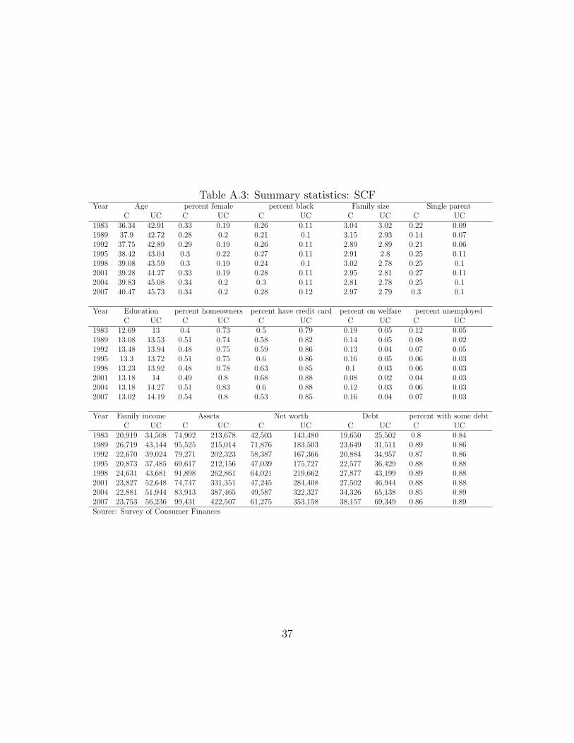
Table A.3: Summary statistics: SCFYear Age percent female percent black Family size Single parent

C UC C UC C UC C UC C UC1983 36.34 42.91 0.33 0.19 0.26 0.11 3.04 3.02 0.22 0.091989 37.9 42.72 0.28 0.2 0.21 0.1 3.15 2.93 0.14 0.071992 37.75 42.89 0.29 0.19 0.26 0.11 2.89 2.89 0.21 0.061995 38.42 43.04 0.3 0.22 0.27 0.11 2.91 2.8 0.25 0.111998 39.08 43.59 0.3 0.19 0.24 0.1 3.02 2.78 0.25 0.12001 39.28 44.27 0.33 0.19 0.28 0.11 2.95 2.81 0.27 0.112004 39.83 45.08 0.34 0.2 0.3 0.11 2.81 2.78 0.25 0.12007 40.47 45.73 0.34 0.2 0.28 0.12 2.97 2.79 0.3 0.1

Year Education percent homeowners percent have credit card percent on welfare percent unemployedC UC C UC C UC C UC C UC

1983 12.69 13 0.4 0.73 0.5 0.79 0.19 0.05 0.12 0.051989 13.08 13.53 0.51 0.74 0.58 0.82 0.14 0.05 0.08 0.021992 13.48 13.94 0.48 0.75 0.59 0.86 0.13 0.04 0.07 0.051995 13.3 13.72 0.51 0.75 0.6 0.86 0.16 0.05 0.06 0.031998 13.23 13.92 0.48 0.78 0.63 0.85 0.1 0.03 0.06 0.032001 13.18 14 0.49 0.8 0.68 0.88 0.08 0.02 0.04 0.032004 13.18 14.27 0.51 0.83 0.6 0.88 0.12 0.03 0.06 0.032007 13.02 14.19 0.54 0.8 0.53 0.85 0.16 0.04 0.07 0.03

Year Family income Assets Net worth Debt percent with some debtC UC C UC C UC C UC C UC

1983 20,919 34,508 74,902 213,678 42,503 143,480 19,650 25,502 0.8 0.841989 26,719 43,144 95,525 215,014 71,876 183,503 23,649 31,511 0.89 0.861992 22,670 39,024 79,271 202,323 58,387 167,366 20,884 34,957 0.87 0.861995 20,873 37,485 69,617 212,156 47,039 175,727 22,577 36,429 0.88 0.881998 24,631 43,681 91,898 262,861 64,021 219,662 27,877 43,199 0.89 0.882001 23,827 52,648 74,747 331,351 47,245 284,408 27,502 46,944 0.88 0.882004 22,881 51,944 83,913 387,465 49,587 322,327 34,326 65,138 0.85 0.892007 23,753 56,236 99,431 422,507 61,275 353,158 38,157 69,349 0.86 0.89Source: Survey of Consumer Finances

37

Table A.4: Evolution of Food Consumption and Income Volatility, allowing for state fixed effectsand cohort dummies, biennial sample, 1980 to 2004.

(1) (2) (3) (4) (5) (6) (7)food income food food income food income

Year/1000 1.525*** 7.295*** 1.520*** 1.448*** 6.867*** 2.876* 13.948***(0.504) (1.486) (0.505) (0.505) (1.482) (1.696) (5.157)

Year > 1992 -0.006 0.064*** -0.006 -0.006 0.065*** -0.010 0.062***(0.007) (0.022) (0.007) (0.007) (0.022) (0.007) (0.022)

Black/Hispanic 0.066*** 0.092*** 0.066*** 0.064*** 0.086*** 0.065*** 0.085***(0.010) (0.027) (0.010) (0.010) (0.027) (0.010) (0.027)

Education< 13 0.014*** 0.044*** 0.014*** 0.014*** 0.045*** 0.017*** 0.050***(0.005) (0.016) (0.005) (0.005) (0.016) (0.005) (0.016)

Age -0.003 -0.027*** -0.003 -0.003 -0.026*** -0.009*** -0.040***(0.002) (0.006) (0.002) (0.002) (0.006) (0.003) (0.009)

Age2 0.000 0.000*** 0.000 0.000 0.000*** 0.000*** 0.000***(0.000) (0.000) (0.000) (0.000) (0.000) (0.000) (0.000)

Change in marital status 0.104*** 0.240*** 0.104*** 0.104*** 0.234*** 0.104*** 0.234***(0.012) (0.030) (0.012) (0.012) (0.030) (0.012) (0.030)

Change in number of adults -0.005 -0.012(0.005) (0.011)

Change in number of kids -0.001 -0.007(0.004) (0.011)

Constant -2.830*** -13.646*** -2.820*** -2.679*** -12.821*** -5.598* -26.797***(1.003) (2.943) (1.003) (1.003) (2.933) (3.353) (10.191)

Observations 33,652 33,652 33,652 33,594 33,594 33,594 33,594State FE No No No Yes Yes Yes YesCohort dummies No No No No No Yes YesAdjusted R2 0.0104 0.0108 0.0104 0.0126 0.0142 0.0152 0.0148Robust, clustered at household level, standard errors in parentheses;*** p<0.01, ** p<0.05, * p<0.1Source: Authors’ calculations based on PSID and SCF data as described in the text.

38

Table A.5: Effect of Liquidity Constraints and Income Uncertainty on Volatility of Consumption,by education, biennial sample, 1980 to 2004.

(1) (2) (3) (4) (5) (6) (7) (8) (9)all ed < 13 ed ≥ 13 all ed < 13 ed ≥ 13 all ed < 13 ed ≥ 13

Year/1000 1.128** 1.174 1.039* 0.514 -0.101 0.934 0.268 -0.135 0.522(0.496) (0.798) (0.628) (0.512) (0.830) (0.650) (0.501) (0.820) (0.630)

Year > 1992 -0.010 -0.012 -0.008 -0.007 -0.008 -0.006 -0.010 -0.011 -0.008(0.007) (0.011) (0.009) (0.007) (0.011) (0.009) (0.007) (0.011) (0.009)

(σYh,t)

2 0.052*** 0.046*** 0.056*** 0.062*** 0.051*** 0.068***(0.004) (0.005) (0.007) (0.008) (0.009) (0.011)

Pr( denied credit) 0.222*** 0.265*** 0.181*** 0.215*** 0.242*** 0.187***(0.024) (0.036) (0.032) (0.025) (0.036) (0.034)

Pr( denied credit)× (σYh,t)

2 -0.051** -0.023 -0.075**(0.024) (0.029) (0.035)

Black/Hispanic 0.061*** 0.066*** 0.055*** 0.024** 0.025 0.019 0.025** 0.025 0.023(0.010) (0.014) (0.012) (0.011) (0.016) (0.015) (0.011) (0.015) (0.014)

Education<13 0.012** 0.000 -0.000(0.005) (0.005) (0.005)

Constant -2.116** -2.178 -1.952 -0.977 0.238 -1.804 -0.493 0.303 -0.991(0.985) (1.585) (1.246) (1.016) (1.644) (1.290) (0.994) (1.625) (1.249)

Observations 33,652 14,683 18,969 33,652 14,683 18,969 33,652 14,683 18,969Adjusted R2 0.036 0.029 0.043 0.015 0.016 0.013 0.040 0.034 0.046

The effect of (σYh,t)

2 is the same across groups (p-value) 0.229

The effect of Pr( denied credit) is the same across groups (p-value) 0.269

The effect of Pr( denied credit× (σYh,t)

2 is the same across groups (p-value) 0.249

Robust, clustered at household level, standard errors in parentheses;*** p<0.01, ** p<0.05, * p<0.1Source: Authors’ calculations based on PSID and SCF data as described in the text.

39

Table A.6: Estimating the Demand for Food in the PSID: The budget elasticity of Food with respect to total NondurableConsumption.

(1) (2) (3) (4) (5) (6) (7) (8)years of data used: 1999-2009 1999-2009 1999-2009 1999-2009 2005-2009 2005-2009 2005-2009 2005-2009

ln(ND1999) 0.741*** 0.681** 0.810*** 0.734*** 0.850***(0.260) (0.280) (0.254) (0.236) (0.201)

ln(ND2005) 0.516*** 0.863*** 0.783***(0.155) (0.268) (0.255)

Observations 20,853 20,853 20,853 20,853 10,718 10,718 10,718 10,718R-squared 0.606 0.595 0.614 0.613 0.609 0.477 0.415 0.436Underid test 8.351 7.654 9.697 9.075 16.72 15.69 9.481 9.843p-value 0.820 0.663 0.406 0.028 0.001 0.109 0.009 0.020Hansen J overid test 10.80 6.262 7.221 2.207 0.227 9.830 0.00484 1.688p-value 0.546 0.713 0.287 0.332 0.893 0.364 0.945 0.430weak id Cragg-Donald Wald F statistic 0.471 0.612 1.115 4.461 4.689 0.754 5.384 2.768elastcity is time invariant (p-value) 0.0796 0.0639 0.0917 - - 0.592 - -elastcity is edu invariant (p-value) 0.0423 0.0456 - - - 0.117 - -elastcity is kid invariant (p-value) 0.215 - - - - 0.408 - -time varying elasticity Yes Yes Yes No No Yes No Noelasticity varies with education Yes Yes No Yes Yes Yes No Noelasticity varies with number of children Yes No No No No Yes No Yes

Note 1: This table reports IV estimates of the demand equation for (the logarithm of) food spending in PSID. We instrument the logof total nondurable expenditure, defined below, (and its interactions with time, education, and kids dummies) with the cohort-education-yearspecific average of the log of the husband’s hourly wage and the cohort-education-year specific average of the log of the wife’s hourly wage(and their interactions with time, education, and kids dummies). Robust, clustered at household level, standard errors in parentheses;*** p<0.01, ** p<0.05, * p<0.1.Note 2: ln(ND1999) is defined as ND expenditure, given available expenditure data as of 1999 forward, on the following categories:expenditure on food at home and away from home, food stamps, childcare, utilities, gasoline, transportation, home and auto insurance,and vehicle repair.ln(ND2005) includes ND expenditure given available expenditure data as of 2005 forward. It includes categories in 1999 definition, plusexpenditure on clothing, home repair, furniture, trips, and other recreation activities.

40

Figure A.1: Proportion of liquidity constrained households, by wealth

.1.2

.3.4

.5

1980 1990 2000 2010year

net non−housing wealth>0 net non−housing wealth<=0

Source: Survey of Consumer Finances.

41

Figure A.2: Increase in average and median debt, in thousands, 1983 dollars

1020

3040

50

1980 1990 2000 2010year

mean debt median debt if debt>0

Source: Survey of Consumer Finances.

Figure A.3: Evolution of Financial Net Worth, in thousands, 1983 dollars

020

000

4000

060

000

1980 1990 2000 2010year

25th percentile 50th percentile75th percentile

Source: Survey of Consumer Finances.

42

Figure A.4: Evolution of Nonfinancial Net Worth, in thousands, 1983 dollars

050

000

1000

00

1980 1990 2000 2010year

25th percentile 50th percentile75th percentile

Source: Survey of Consumer Finances.

Figure A.5: Percent of Households with net assets less than two months of income.

.1.2

.3.4

1980 1990 2000 2010year

white nonwhite

Source: Survey of Consumer Finances.

43

Figure A.6: Average mortgage vs. non-mortgage debt, in 1983 dollars

010

2030

40

1980 1990 2000 2010year

mortgage non−mortgage

Source: Survey of Consumer Finances.

Figure A.7: Proportion of liquidity constrained households, by race and education

.1.2

.3.4

.5

1980 1990 2000 2010year

white, <12 years

white, 12−15 years

white, 16+ years

.1.2

.3.4

.5

1980 1990 2000 2010year

black, <12 years

black, 12−15 years

black, 16+ years

Source: Survey of Consumer Finances.

44

Figure A.8: Proportion of households applying for credit and rejected, by race andeducation

0.2

.4.6

.8

1980 1990 2000 2010year

% applied, black

% applied, white

% rejected, black

% rejected, white

<12 years

0.2

.4.6

.8

1980 1990 2000 2010year

% applied, black

% applied, white

% rejected, black

% rejected, white

12−15 years

0.2

.4.6

.8

1980 1990 2000 2010year

% applied, black

% applied, white

% rejected, black

% rejected, white

16+ years

Source: Survey of Consumer Finances.

Figure A.9: Proportion of constrained household, by income quintile

.05

.1.1

5.2

.25

.3

1980 1990 2000 2010year

Lowest 2nd3rd 4thHighest

Source: Survey of Consumer Finances.

45

Figure A.10: Proportion of constrained households, by demographic group

.1.2

.3.4

.5

1980 1990 2000 2010year

all households

.1.2

.3.4

.5

1980 1990 2000 2010year

married single parent

.1.2

.3.4

.5

1980 1990 2000 2010year

white black/Hispanic.1

.2.3

.4.5

1980 1990 2000 2010year

college no college

Source: Survey of Consumer Finances.

Figure A.11: Percentage with net assets less than two months’ income, by demo-graphic group

.1.2

.3.4

.5

1980 1990 2000 2010year

all households

.1.2

.3.4

.5

1980 1990 2000 2010year

married single parent

.1.2

.3.4

.5

1980 1990 2000 2010year

white black/Hispanic

.1.2

.3.4

.5

1980 1990 2000 2010year

college no college

Source: Survey of Consumer Finances.

46

Figure A.12: Median net assets to income ratio, by demographic group

0.2

.4.6

.81

1980 1990 2000 2010year

all households

0.2

.4.6

.81

1980 1990 2000 2010year

married single parent

0.2

.4.6

.81

1980 1990 2000 2010year

white black/Hispanic0

.2.4

.6.8

1

1980 1990 2000 2010year

college no college

Source: Survey of Consumer Finances.

Figure A.13: Mean Estimated Probabilities in the SCF and the PSID

.18

.2.2

2.2

4.2

6.2

8

1982 1986 1990 1994 1998 2002year

PSID SCF

Source: Author estimates from Survey of the Consumer Finances and the Panel Study of IncomeDynamics.

47

Figure A.14: Proportion of constrained household, by demographic group in PSID

.1.2

.3.4

.5.6

1982 1986 1990 1994 1998 2002year

white, <12 years

white, 12−15 years

white, 16+ years

.1.2

.3.4

.5.6

1982 1986 1990 1994 1998 2002year

black, <12 years

black, 12−15 years

black, 16+ years

Source: Panel Study of Income Dynamics.

48

References

Mark A. Aguiar and Mark Bils. Has Consumption Inequality Mirrored Income In-equality? NBER working papers, National Bureau of Economic Research, Inc,February 2011.

Sule Alan, Orazio Attanasio, and Martin Browning. Estimating Euler Equationswith Noisy Data: Two Exact GMM Estimators. Journal of Applied Econometrics,24(2):309–324, 2009.

Sule Alan, Kadir Atalay, and Thomas F. Crossley. Euler Equation Estimation onMicro Data. Ko University-TUSIAD Economic Research Forum Working Papers1221, Koc University-TUSIAD Economic Research Forum, Aug 2012.

Manuel Arellano and Olympia Bover. Another Look at the Instrumental VariablesEstimation of Errorcomponents Models. Journal of Econometrics, 68:29–51, 1995.

Orazio Attanasio. Consumption. In J.B. Taylor and M. Woodford, editors, Handbookof Macroeconomics, Vol. 1, pages 741–812. Elsevier Science B.V., 1999.

Orazio Attanasio and Hamish Low. Estimating Euler Equations. Review of EconomicDynamics, 7:406–435, 2004.

Orazio Attanasio and Guglielmo Weber. Is Consumption Growth Consistent withIntertemporal Optimization? Evidence from the Consumer Expenditure Survey.Journal of Political Economy, 103(6):1121–1157, 1995.

Orazio Attanasio, Pinelopi K. Goldberg, and Ekaterini Kyriazidou. Credit Con-straints in the Market for Consumer Durables: Evidence from Micro Data on CarLoans. International Economic Review, 49(2), 2008.

Orazio Attanasio, Erik Hurst, and Luigi Pistaferr. The evolution of income, consump-tion, and leisure inequality in the us, 1980-2010. In Improving the Measurementof Consumer Expenditures. 2013.

James Banks, Richard Blundell, and Arthur Lewbel. Quadratic Engel Curves andConsumer Demand. The Review of Economics and Statistics, LXXIX(4):527–539,1997.

Richard Blundell, Luigi Pistaferri, and Ian Preston. Consumption inequality andpartial insurance. American Economic Review, 98(5):1887–1921, 2008.

49

Richard Blundell, Luigi Pistaferri, and Itay Saporta-Eksten. Consumption inequalityand family labor supply. NBER Working Papers, 2012.

John Bound, Charles Brown, Greg J. Duncan, and Willard Rodgers. Evidence onthe Validity of Cross-Sectional and Longitudinal Labor Market Data. Journal ofLabor Economics, 12:345–368, 1994.

Martin Browning and Thomas Crossley. Are two cheap, noisy measures better thanone expensive. American Economic Review, 2009.

Martin Browning and Annamaria Lusardi. Household Saving: Micro Theories andMicro Facts. Journal of Economic Literature, 34:1797–1855, 1996.

Christopher Carroll. The Buffer-Stock Theory of Saving: Some MacroeconomicEvidence. Brookings Papers on Economic Activity, (2):61–135, 1992.

Christopher Carroll. Death to the log-linearized consumption Euler equation! 2001.

Thomas F. Crossley and Hamish W. Low. Is The Elasticity Of Intertemporal Sub-stitution Constant? Journal of the European Economic Association, 9(1):87–105,02 2011.

Molly Dahl, Thomas DeLeire, and Jonathan Schwabish. Year-to-year variability inworker earnings and in household incomes: Estimates from administrative data.Technical report, Congressional Budget Office, 2008.

Steven Davis and James Kahn. Interpreting the Great Moderation: Changes inVolatility of Economic Activity at the Macro and Micro Levels. The Journal ofEconomic Perspectives, 22(4):155–180, 2008.

Jason DeBacker, Bradley Heim, Vasia Panousi, Shanthi Ramnath, and Ivan Vidan-gos. Rising inequality: Transitory or permanent? New evidence from a panel ofU.S. tax returns. Brookings Papers on Economic Activity, Spring 2013.

Karen Dynan, Douglas Elmendorf, and Daniel Sichel. The Evolution of HouseholdIncome Volatility. The B.E. Journal of Economic Analysis and Policy: Advances,December 2012.

Olga Gorbachev. Did household consumption become more volatile? AmericanEconomic Review, 101, 2011.

Peter Gottschalk and Robert Moffitt. The Rising Instability of U.S. Earnings. Journalof Economic Perspectives, 23(4):3–24, 2009.

50

David B. Gross and Nicholas S. Souleles. Do Liquidity Constraints and InterestRates Matter for Consumer Behavior? Evidence from Credit Card Data. QuarterlyJournal of Economics, 117(1):149–185, 2002.

Craig Gundersen and James P. Ziliak. The age gradient in food stamp programparticipation: Does income volatility matter? In D. Joliffe and J. Ziliak, editors,Trends in Income and Consumption Volatility, 1970-2000. Upjohn Institute forEmployment Research, 2008.

Fatih Guvenen. Learning Your Earning: Are Labor Income Shocks Really VeryPersistent? American Economic Review, 97(3):687–712, June 2007.

Fatih Guvenen, Serdar Ozkan, and Jae Song. The nature of countercyclical incomerisk. NBER Working Paper Series, 2012.

Rong Hai, Dirk Krueger, and Andrew Postlewaite. On the Welfare Cost of Consump-tion Fluctuations in the Presence of Memorable Goods. NBER Working Papers19386, National Bureau of Economic Research, Inc, August 2013.

Tullio Jappelli. Who is Credit Constrained in the U. S. Economy? Quarterly Journalof Economics, 105(1):219–234, 1990.

Tullio Jappelli and Luigi Pistaferri. The Consumption Response to Income Changes.NBER Working Paper Series, WP15739, 2010.

Tullio Jappelli, Jorn-Steffen Pischke, and Nicholas S. Souleles. Testing for LiquidityConstraints in Euler Equations with Complementary Data Sources. The Reviewof Economics and Statistics, 80(2):251–262, 1998.

Shane T. Jensen and Stephen H. Shore. Changes in the distribution of incomevolatility. http://www.econ.jhu.edu/People/Shore/Research/jensenshore_

econ.pdf, 2008.

Benjamin Keys. Income volatility and food assistance in the united states. In D. Jo-liffe and J. Ziliak, editors, Trends in Income and Consumption Volatility, 1970-2000. Upjohn Institute for Employment Research, 2008.

Bonggeun Kim and Gary Solon. Implications of Mean-Reverting Measurement Errorfor longitudinal studies of wages and employment. The Review of Economics andStatistics, 87(1):193–196, 2005.

51

Yong-Seong Kim and Frank P. Stafford. The quality of PSID income data in the1990’s and beyond. PSID Technical Series, 2000.

Dirk Krueger and Fabrizio Perri. Does Income Inequality Lead to ConsumptionInequality? Evidence and Theory. Review of Economic Studies, 73(1):163–193,2006.

Suzanne Lindamood, Sherman D. Hanna, and Lan Bi. Using the Survey of ConsumerFinances: Methodological Considerations and Issues. Journal of Consumer Affairs,41(2):195–214, 2007.

Robert Lucas. Models of Business Cycle. Oxford: Basil Blackwell, 1987.

Thomas E. MaCurdy. The Use of the Time-Series Processes to Model the ErrorStructure of Earnings in a Longitudinal Data-Analysis. Journal of Econometrics,18(1):83–114, 1982.

Costas Meghir and Luigi Pistaferri. Chapter 9 - earnings, consumption and life cyclechoices. volume 4, Part B of Handbook of Labor Economics, pages 773 – 854.Elsevier, 2011.

Costas Meghir and Guglielmo Weber. Intertemporal nonseparability or borrowingrestrictions? a disaggregate analysis using a u.s. consumption panel. Econometrica,64(5):1151–1181, 1996.

Robert A. Moffitt and Peter Gottschalk. Trends in the Transitory Variance of MaleEarnings in the U.S., 1970-2004. Working Paper 16833, National Bureau of Eco-nomic Research, February 2011.

Stephen J. Nickell. Biases in Dynamic Models with Fixed Effects. Econometrica, 49(6):1417–26, 1981.

Giorgio Primiceri and Thijs vanRens. Heterogeneous Life-Cycle Profiles, IncomeRisk and Consumption Inequality. Journal of Monetary Economics, 56(1):20–39,2009.

Ricardo Reis. The time-series properties of aggregate consumption: Implications forthe costs of fluctuations. Journal of the European Economic Association, 7(4):722–753, 06 2009.

David M. Roodman. A Note on the Theme of Too Many Instruments. OxfordBulletin of Economics and Statistics, 71(1):135–158, 2009.

52

David Runkle. Liquidity Constraints and the Permanent-Income Hypothesis. Journalof Monetary Economics, 27:73–98, 1991.

John Sabelhaus and Jae Song. Earnings volatility across groups and time. NationalTax Journal, June 2009.

Amartya Sen. Equality of what? In S. McMurrin, editor, The Tanner Lectures onHuman Values, number 8. Cambridge: Cambridge University Press, 1980.

M. Stone. Cross-validatory choice and assessment of statistical predictions. Journalof the Royal Statistical Society. Series B (Methodological), 36(2):pp. 111–147, 1974.

Frank Windmeijer. A finite sample correction for the variance of linear efficienttwo-step GMM estimators. Journal of Econometrics, 2005.

Stephen Zeldes. Optimal Consumption with Stochastic Income: Deviations fromCertainty Equivalence. Quarterly Journal of Economics, 104(2):275–298, 1989a.

Stephen Zeldes. Consumption and Liquidity Constraints: An Empirical Investiga-tion. Journal of Political Economy, 97(2):305–346, 1989b.

53