cranfield university, silsoe, institute of water and the
TRANSCRIPT

Cranfield University, Silsoe, Institute of Water and the Environment
MSc Thesis
Academic Year: 2005-2006
Manuel Beltrán Miralles
DEVELOPMENT OF WATER BALANCE MODELS OF
DOÑANA MARSHES USING REMOTE SENSING
DETERMINATION OF THEIR FLOOD EXTENT.
Supervisors: Professor Sue White
Professor Javier Bustamante Díaz
Word Length: 9,993
Date of Presentation: 6th September 2006
This thesis is submitted in partial fulfillment of the requirements for the Degree of Master of Science
© Cranfield University (2006). All rights reserved. No part of this publication may be reproduced without
the written permission of the copyright holder.
brought to you by COREView metadata, citation and similar papers at core.ac.uk
provided by Digital.CSIC

ii
iii
ABSTRACT
The Doñana Biological Station monitors the flood extent of Doñana marshes, in
Southwestern Spain, using Landsat images. These data have been used to develop
different models that permit simulation of the variation in the flood extent in the
marshes throughout the hydrologic year, the models being based on a daily balance of
water inputs and outputs. Five different models were developed using data for the
period 1994-2004. Direct precipitation and evaporation were estimated using climate
data. The absorption of water by the marshes at the beginning of the hydrologic year
(Absmax) was calibrated in one model (model A) and estimated in the others (models B-
156, B-420, C-156 and C-420). River flow inputs were modeled using a conceptual
rainfall-runoff model (Témez model). The Témez model parameters were calibrated in
two models (B-156 and B-420) without using runoff records. River flow inputs in the
other models were estimated using runoff parameters from a nearby catchment (the
Meca River) for model A and not considered for models C-156 and C-420. The
goodness of fit of the models was assessed using a weighted R2 (wR
2). The analyses
indicate that the calibration of the Témez model without using runoff records does not
provide the best results, although it must be possible to obtain reasonable results with a
longer and more homogeneous period of study. The use of Témez model parameters
calibrated for the Meca River catchment does not permit an accurate calibration of
Absmax. In addition, the analyses indicate that it is possible to develop a model with a
high goodness of fit using data from a single meteorological station located in the
marshes (station 5858) and considering runoff as null, although further analyses are
required to asses how this model would simulate the different phases of the hydrologic
cycle of the marshes.

iv

v
ACKNOWLEDGEMENTS
This MSc thesis could not have been possible without many different people whose
support and help I would like to acknowledge.
To Sue White and Javier Bustamante, my supervisors in, respectively, Cranfield
University and the Doñana Biological Station (EBD), whose help and knowledge have
made possible this thesis.
To the people of the GIS and Remote Sensing Laboratory of the EBD: Ricardo Diaz-
Delgado, Fernando Pacios and, especially, David Aragonés, to whom I will always be
grateful for his pieces of advice and for his huge patience and support.
Thanks to Christophe Sannier, from Cranfield University, for his advice in GIS-related
issues. To Tim Hess, from Cranfield University, Inmaculada Bautista, from the
Polytechnic University of Valencia, and Francisco Domingo, from CSIC, for their
advice in topics regarding evapotranspiration. To Rafael García, from the Polytechnic
University of Valencia, and Victor Castillo, from CSIC, thanks for their information
about hydrological models employed in Spain.
Thanks to Ramon Soriguer for showing me that incredible place Doñana is, and to Juan
José Chans and Carlos Urdiales, who answered my doubts about the hydrology of the
area.
To my family: Susi, Mano and Vicente. There are so many things I want to thank you
for!
And finally, to those butterflies that flapping their wings have prompted in one way or
another this project and my stay in Seville during these three months.

vi

vii
TABLE OF CONTENTS
ABSTRACT
ACKNOWLEDGEMENTS
TABLE OF CONTENTS
LIST OF TABLES
LIST OF FIGURES
LIST OF SYMBOLS
1. INTRODUCTION
1.1. Aim and objectives
2. LITERATURE REVIEW
2.1. Black-box and water balance models
2.2. Selection of the Rainfall-Runoff model
2.3. Potential Evapotranspiration.
2.4. Model calibration and assessment
3. THE STUDY AREA AND AVAILABLE DATA
3.1. Study area
3.2. Available data
3.2.1. Flood extent data
3.2.2. Meteorological data
3.2.3. Digital Elevation Models
3.2.4. Watercourses coverage
3.2.5. Catchment area
3.2.6. Lithology maps
3.2.7. Land Use/ Land Cover map
4. METHODOLOGY
4.1. Infilling of climate data gaps
4.2. Water volume calculation
iii
v
vii
xi
xiii
xvii
1
2
3
3
3
5
6
9
9
12
12
12
12
13
13
13
13
15
19
20

viii
4.3. Absmax calculation.
4.4. Estimation of Témez model inputs.
4.5. Time of concentration calculation.
4.6. Data distribution for calibration and validation.
5. CALIBRATION
5.1. Model A calibration
5.2. Models B calibration
5.2.1. Absmax calculation
5.2.2. Rainfall-Runoff model parameters calculation
a) Maximum soil moisture storage capacity (Smax)
b) Maximum infiltration capacity (Imax)
c) Aquifer discharge parameter (α)
5.2.3. Calibration and sensitivity analysis.
5.2.4. Final parameter values selected
6. RESULTS
6.1. Relationship “flood extent-water volume”
6.2. Time of concentration
6.3. Models validation
6.3.1. Model A
6.3.2. Model B-156
6.3.3. Model B-420
6.3.4. Model C-156
6.3.5. Model C-420
6.3.6. Phases of the marshes annual hydrological cycle
7. DISCUSSION
7.1. Model A
7.2. Models B
7.3. Models C
21
22
22
24
25
25
28
29
30
30
32
33
33
34
35
35
37
38
39
40
41
42
43
44
47
48
50
51

ix
7.4. Analysis of the residuals in relation to the phases of the
marshes annual hydrological cycle.
7.5. Estimation of other variables.
8. CONCLUSION AND RECOMMENDATIONS
9. REFERENCES
10. APPENDICES
A. Témez Model Equations
B. Hargreaves Equation
C. Relief Of The Catchment Of Doñana Marshes
D. Lithology Map Of The Catchment Of Doñana Marshes
E. Land Use/Land Cover Map Of The Catchment Of
Doñana Marshes
F. Procedure Followed For The Infilling Of The
Meteorological Data Gaps
G. Watercourses Employed For The Calculation Of The
Time Of Concentration
H. Data Employed And Calculations Conducted For The
Estimation Of Smax From Published Soil Analyses
I. Thiessen Calculations
J. Simulation Of The Daily Flood Extent For The Different
Models Developed.
K. Cd Contents Description
52
52
55
57
63
65
66
67
68
69
74
75
77
78
88

x

xi
LIST OF TABLES
Table 2.1- Parameters employed by the Témez model
Table 4.1- Daily water balance used to simulate the variation in the
volume of water contained in the marshes throughout the
hydrologic year.
Table 4. 2- Dates for which the volume was calculated from satellite
images. The number contained in each cell indicates the
day the image was taken for a certain month (columns) and
year (row).
Table 4.3- Meteorological stations and Thiessen coefficients obtained
for the catchment existing before 25th April 1998.
Table 4.4- Meteorological stations and Thiessen coefficients for the
catchment existing after 25th April 1998.
Table 4.5- Precipitation of each hydrologic year and set to which it
was assigned (calibration or validation).
Table 5.1- Values of Témez parameters calibrated for the Meca River
by Verdú (2004).
Table 5.2- Sequences employed for the calibration of models B-156
and B-420.
Table 5.3- Possible range of values selected for the estimation of the
Témez parameters in model B-156 and B-420 calibration,
and values selected prior to the sensitivity analysis.
Table 5.4- Value of Smax assigned to each land use present in the
catchment.
Table 5.5- Smax values estimated for the catchment.
Table 5.6- Values of Imax assigned to each lithology class present in
the area.
Table 5.7- Imax values estimated for the catchment.
Table 5. 8- Values of Absmax and Témez parameters employed in the
calibration of models B-156 and B-420 and sum of squares
of the residuals obtained.
5
16
20
23
23
24
26
29
30
31
32
32
32
34

xii
Table 6.1- Data used in the calculation of the time of concentration of
the main watercourses using Kirpich equation.
Table 6.2- Results from model A validation.
Table 6.3- Results from model B-156 validation.
Table 6.4- Results from model B-420 validation.
Table 6.5- Results from model C-156 validation.
Table 6.6- Results from model C-420 validation.
Table 6.7- Results obtained from the analysis of each of the phases of
hydrological cycle of the marshes for models A, B-156 and
B-420.
Table 6.8- Results obtained from the analysis of each of the phases of
hydrological cycle of the marshes for models C-156 and C-
420
Table 7.1- Summary of the characteristics of the models developed.
Table 7.2- Summary of the results obtained from the validation of the
different models.
Table 7.3- Values of the Témez parameters used in models A, B-156
and B-420.
Table F.1- Characteristics of all pluviometric stations from which data
was acquired.
Table F.2- Characteristics of all thermometric stations from which
data was acquired.
Table H.1- Soil properties used for Smax calculation (1/2).
Table H.2- Soil properties used for Smax calculation (2/2).
Table I.1- Thiessen calculations for Pluviometric stations in the
catchment before 25/08/1998.
Table I.2- Thiessen calculations for Pluviometric stations in the
catchment after 25/08/1998.
Table I.3- Thiessen calculations for Thermometric stations in the
catchment before 25/08/1998.
Table I.4- Thiessen calculations for Thermometric stations in the
catchment before 25/08/1998.
37
39
40
41
42
43
44
45
47
47
50
69
70
75
76
77
77
77
77

xiii
LIST OF FIGURES
Figure 1.1- Example of a situation of minimum flood extent (left) and
maximum flood extent (right) in Doñana marshes.
Figure 2.1- Témez model diagram (modified from Oliveira, 1998).
Figure 3.1- Location of Doñana National Park.
Figure 3.2- Areas designated as National Park and Natural Park and
marshes location.
Figure 3.3- Catchments of the main runoff contributors to Doñana
marshes.
Figure 4.1- Water balance and main variables employed in the models.
Figure 4.2- Area considered as marshes in the study and areas flooded
during the hydrologic year 2002-2003.
Figure 4.3- Location, altitude and code of the meteorological stations
employed.
Figure 5.1- Location of the Meca River and Doñana.
Figure 5.2- Correlation between observed and simulated flood extents
obtained from the calibration of model A.
Figure 5.3- Distribution of the residuals obtained from the calibration
of model A.
Figure 5.4- Maximum soil moisture storage capacity (mm) in the
catchment.
Figure 5.5- Maximum infiltration capacity (mm) in the catchment.
Figure 6.1- Linear function showing the relationship between S3/2 and
V from which the function S=f (V2/3) was derived.
Figure 6.2- Third degree polynomial function showing the extension
of the area flooded in the marshes in function of the
volume of water contained by them.
Figure 6.3- Distribution of the residuals of the linear and polynomial
functions.
Figure 6.4- Correlation obtained from model A validation.
Figure 6.5- Residual plot obtained from the validation of model A.
Figure 6.6- Correlation obtained from model B-156 validation.
1
4
9
9
11
17
18
19
25
27
27
31
33
35
36
37
39
39
40

xiv
Figure 6.7- Residual plot obtained from the validation of model
B-156.
Figure 6.8- Correlation obtained from model B-420 validation.
Figure 6.9- Residual plot obtained from the validation of model
B-420.
Figure 6.10- Correlation obtained from model C-156 validation.
Figure 6.11- Residual plot obtained from the validation of model
C-156.
Figure 6.12- Correlation obtained from model C-420 validation.
Figure 6.13- Residual plot obtained from the validation of model
C-420.
Figure 7.1- Maximum flood extent occurred during the hydrologic
year 1998-1999.
Figure 7.2- Flood extents simulated by the model B-156 and observed
(estimated from the satellite images) for the hydrologic
year 1998-1999.
Figure 7.3- Flood extents simulated by the model B-420 and observed
(estimated from the satellite images) for the hydrologic
year 1998-1999.
Figure F.1- Location of the thirteen pluviometric stations.
Figure F.2- Location of the eight thermometric stations.
Figure F.3- Degree of data completeness of the meteorological
stations during the period 1994-1999. Periods in white
represent data gaps in the acquired data of at least one
month.
Figure F.4- Degree of data completeness of the meteorological
stations during the period 2000-2004. Periods in white
represent data gaps in the acquired data of at least one
month.
Figure J.1- Flood extent simulated by model A for the hydrologic year
1996-1997.
40
41
41
42
42
43
43
48
49
49
71
71
72
73
78
xv
Figure J.2- Flood extent simulated by model A for the hydrologic year
1998-1999.
Figure J.3- Model A flood extent simulation for the hydrologic year
2000-2001.
Figure J.4- Model A flood extent simulation for the hydrologic year
2002-2003.
Figure J.5- Model A flood extent simulation for the hydrologic year
2003-2004.
Figure J.6- Model B-156 flood extent simulation for the hydrologic
year 1996-1997.
Figure J.7- Model B-156 flood extent simulation for the hydrologic
year 1998-1999.
Figure J.8- Model B-156 flood extent simulation for the hydrologic
year 2000-2001.
Figure J.9- Model B-156 flood extent simulation for the hydrologic
year 2002-2003.
Figure J.10- Model B-156 flood extent simulation for the hydrologic
year 2003-2004.
Figure J.11- Model B-420 flood extent simulation for the hydrologic
year 1996-1997.
Figure J.12- Model B-420 flood extent simulation for the hydrologic
year 1998-1999.
Figure J.13- Model B-420 flood extent simulation for the hydrologic
year 2000-2001.
Figure J.14- Model B-420 flood extent simulation for the hydrologic
year 2002-2003.
Figure J.15- Model B-420 flood extent simulation for the hydrologic
year 2003-2004.
Figure J.16- Model C-156 flood extent simulation for the hydrologic
year 1996-1997.
Figure J.17- Model C-156 flood extent simulation for the hydrologic
year 1998-1999.
78
79
79
79
80
80
80
81
81
82
82
82
83
83
84
84

xvi
Figure J.18- Model C-156 flood extent simulation for the hydrologic
year 2000-2001.
Figure J.19- Model C-156 flood extent simulation for the hydrologic
year 2002-2003.
Figure J.20- Model C-156 flood extent simulation for the hydrologic
year 2003-2004.
Figure J.21- Model C-420 flood extent simulation for the hydrologic
year 1996-1997.
Figure J.22- Model C-420 flood extent simulation for the hydrologic
year 1998-1999.
Figure J.23- Model C-420 flood extent simulation for the hydrologic
year 2000-2001.
Figure J.24- Model C-420 flood extent simulation for the hydrologic
year 2002-2003.
Figure J.25- Model C-420 flood extent simulation for the hydrologic
year 2003-2004.
84
85
85
86
86
86
87
87

xvii
LIST OF SYMBOLS
α Aquifer discharge parameter
A Surface runoff
Absmax Maximum amount of water the marshes’ soils can absorb at the
beginning of the hydrologic year
B Baseflow
Bo Initial baseflow
c Surplus parameter
DEM Digital Elevation Model
E Actual evapotranspiration
EP Potential evapotranspiration
ETo Reference evapotranspiration
EU European Union
FAO Food and Agriculture Organization
GIS Geographic Information System
Ii Infiltration in the day i
I Inputs of water to the marshes
Imax Maximum infiltration capacity
IGME Spanish Geological Survey
JPEG Joint Photographic Experts Groups
Kc Crop coefficient
LAST-EBD GIS and Remote Sensing Laboratory of the Doñana Biological
Station
LIDAR Light Detection and Ranging
O Outputs of water from the marshes
P Precipitation
R Total runoff
Rr Runoff required
R2 Coefficient of determination
S Size of the flood extent in the marshes
Si Available moisture in the soil during the day i
Smax Maximum soil moisture storage capacity

xviii
So Initial soil moisture storage capacity
tc Time of concentration
Tmax Maximum temperature
Tmin Minimum temperature
V Volume of water contained in the marshes
Vmax Maximum volume of water the marshes can contain.
w R2 Weighted coefficient of determination
X Surplus flow
Cranfield University at Silsoe Manuel Beltrán Miralles, 2006 1
1. INTRODUCTION
Doñana National Park, located in Southwestern Spain, is a site of international
importance in terms of conservation, designated as a Ramsar Site, a UNESCO Man and
Biosphere Reserve and an EU Special Protection Area for birds. In addition, part of its
adjacent area is designated as Natural Park. These designations have been motivated to
a large extent by the important role that the marshes, largely included within the
National Park boundaries, play in the breeding, staging and wintering of birds (Ramsar,
2002).
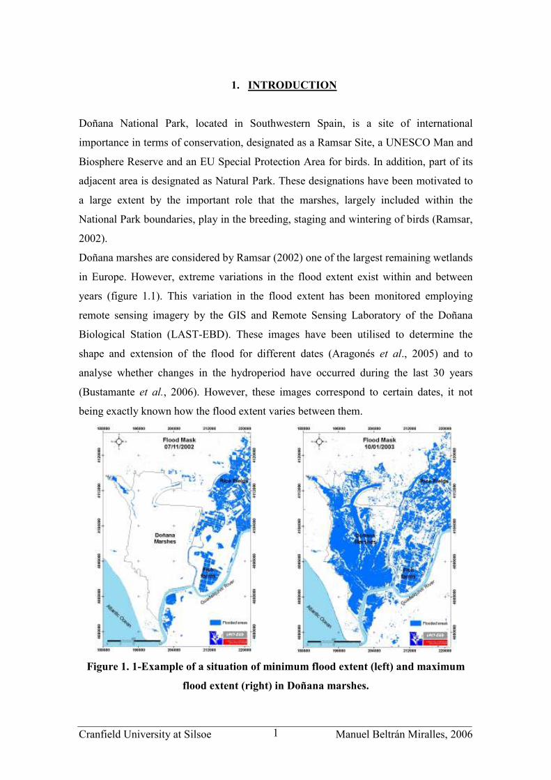
Doñana marshes are considered by Ramsar (2002) one of the largest remaining wetlands
in Europe. However, extreme variations in the flood extent exist within and between
years (figure 1.1). This variation in the flood extent has been monitored employing
remote sensing imagery by the GIS and Remote Sensing Laboratory of the Doñana
Biological Station (LAST-EBD). These images have been utilised to determine the
shape and extension of the flood for different dates (Aragonés et al., 2005) and to
analyse whether changes in the hydroperiod have occurred during the last 30 years
(Bustamante et al., 2006). However, these images correspond to certain dates, it not
being exactly known how the flood extent varies between them.
Figure 1. 1-Example of a situation of minimum flood extent (left) and maximum
flood extent (right) in Doñana marshes.

Cranfield University at Silsoe Manuel Beltrán Miralles, 2006 2
Due to the role the marshes play in the ecology of Doñana, it is important to develop a
model that simulates the variation in the flood extent throughout the year. This can be
obtained employing tools that statistically relate the flood extent to variables such as the
accumulated rainfall, the model developed this way being called a black-box model.
Although these models might provide high accuracy levels, they might poorly simulate
responses to climatic conditions different than those used for their calibration. This is
important in the case of Doñana marshes, since changes in the climatic conditions in the
area for the current century have been predicted (WWF/Adena, 2006). Therefore, a
black-box model calibrated with current climate data may not be applicable in the mid
to long term.
An alternative approach described in the literature is the use of a water balance model,
which requires the calculation of the main inputs and outputs of water to the marshes,
such as precipitation or runoff. The estimation of the latter is carried out by means of a
rainfall-runoff model, generally calibrated with runoff records. In the case of Doñana,
runoff records cannot be employed as they have a low reliability and many data gaps
and because not all runoff inputs to the marshes are measured. These factors would
hinder the accuracy of the rainfall-runoff model that would be calibrated and, therefore,
of the water balance model that would be obtained. However, it might be possible to use
the determination of the flood extent in the marshes by means of satellite images to
calibrate the model, runoff records not being required and an important constraint being
removed in this way.
1.1 Aim and objectives
This paper aims to analyse the feasibility of developing a model for simulating the flood
extent of Doñana marshes using for its calibration flood extent data obtained from
satellite images.
The objectives of the study are:
- Assess the goodness of fit of the models developed for different phases of the
marshes annual hydrological cycle.
- Indicate recommendations for future studies to improve the results obtained in
the paper.

Cranfield University at Silsoe Manuel Beltrán Miralles, 2006 3
2 LITERATURE REVIEW
2.1 Black-box and water balance models.
Some studies exist in the published literature aiming to predict the spatial extent of the
flood in different kinds of wetlands. Gumbritch et al. (2004) developed a statistical
model that permitted the prediction of the maximum area of flooding in the Okavango
delta (Botswana). Roshier et al. (2001) developed models for seven large regions of
Australia relating weather patterns to wetland filling. Liu et al. (2003) developed a
model for predicting the inundation area in the Pantanal wetland (Brazil). All the three
studies used remote sensing applications to determine the flood extent of the different
study sites and were based on the use of black-box models.
Different water balance models have been applied to rivers and wetlands and can be
found in the published literature. Delgado (2005) applied a similar model to the Caroní
River, in Bolivia. Casas and Urdiales (1995) developed a water balance model of
Doñana marshes. This model was based on the estimation of monthly inputs and outputs
and was not calibrated or validated; however, it provides an estimation of the variation
in the volume of water contained in the marshes for different months. In addition,
García et al. (2005) provided a conceptual model of the hydrologic regime of the
marshes and linked it to the vegetation communities present in the area.
2.2 Selection of the Rainfall-Runoff model
A review of different rainfall-runoff models was carried out in order to select a suitable
model for the area. Physically-based models were rejected due to time and data
constraints that made the calibration and estimation of their large number of parameters
unfeasible. Black-box models were not utilised due to the short period of data available
for their calibration and validation (ten years) and due to predicted changes in the future
climatic conditions in the area. A conceptual model was considered the most suitable
option.
Different conceptual models were reviewed from Beven (2001) and from different
studies in Spain. TOPMODEL (see Beven, 2001) was an interesting option due to its
GIS implementation; however, it is not applicable in catchments “subject to strong

Cranfield University at Silsoe Manuel Beltrán Miralles, 2006 4
seasonal drying” (Beven, 2001). Other models, such as the Palmer model (Palmer,
1965), were not suitable since they do not consider baseflow, which is an important
input in this case.
Finally, the Témez model was selected, which is a lumped and deterministic model
developed by Témez (1977) that has been commonly used in Spain and Portugal
(Verdú, 2004; Oliveira, 1998; Ruíz, 2000). The model divides the subsoil of the
catchment into two stores: one unsaturated and superficial and other saturated and
subterranean (Oliveira, 1998).
Figure 2.1 - Témez model diagram (modified from Oliveira, 1998).
The model suits the hydrological situation of the marshes as groundwater emerges to the
surface upstream of the marshes, combining with the surface runoff in the catchment
and reaching the marshes as runoff (figure 2.1).
The Témez model requires setting two initial conditions: the initial soil moisture storage
capacity (So) and initial baseflow (Bo). It also includes four parameters, which normally
need to be calibrated (table 2.1). The model uses precipitation and potential
evapotranspiration as inputs. The model equations are included in the Appendix A.

Cranfield University at Silsoe Manuel Beltrán Miralles, 2006 5
Table 2.1 – Parameters employed by the Témez model.
Parameter Description
Smax Maximum soil moisture storage capacity (mm)
c Surplus parameter
α Aquifer discharge parameter (day-1)
Imax Maximum infiltration capacity (mm)
2.3 Potential Evapotranspiration
Potential evapotranspiration (EP) is defined as: “the amount of water transpired in a
given time by a short green crop, completely shading the ground, of uniform height and
with adequate water status in the soil profile” (Irmak & Haman, 2003). Air temperature
values were the only data available for its calculation, hence the selection of the method
had to be restricted to the so-called air temperature-based methods. Among them, the
Thornwaite equation has been employed before in the area (Casas & Urdiales, 1995;
García et al., 2005). However, this method tends to underestimate EP (García et al.,
2005), underestimation being in some cases close to 40% (Oliveira, 1998).
Many different crops fit into the description of short green crop given in the EP
definition (Irmak & Haman, 2003). To avoid this ambiguity, the concept of reference
evapotranspiration (ETo) was suggested in the late 1970s, it being defined as “the rate of
evapotranspiration from a hypothetical reference crop with an assumed crop height of
0.12 m (4.72 in), a fixed surface resistance of 70 sec m-1 (70 sec 3.2ft
-1) and an albedo
of 0.23, closely resembling the evapotranspiration from an extensive surface of green
grass of uniform height, actively growing, well-watered, and completely shading the
ground” (Irmak & Haman, 2003). Therefore, EP and ETo are similar concepts with the
main difference that the crop of reference is more detailed in the ETo definition.
According to Irmak and Haman (2003), the ETo concept makes easier the calibration of
evapotranspiration equations for a given local climate. Gavilán et al. (2005) conducted
for different areas in Southern Spain a regional calibration of the Hargreaves equation
(Hargreaves & Samani, 1985), which is recommended by the FAO (Allen et al., 1998)
to estimate ETo when air temperature is the only data available. Gavilán et al. (2005)

Cranfield University at Silsoe Manuel Beltrán Miralles, 2006 6
concluded that accurate results can be obtained in the region where Doñana is located
with the Hargreaves equation (1).
ao RTTTT
ET ⋅−⋅++
= 5.0
minmaxminmax )()8.17
2(0023.0 (1)
where ETo is expressed in mm day-1, Tmax and Tmin are, respectively, the maximum and
minimum temperatures, both expressed in ºC and Ra is the water equivalent of the
extraterrestrial radiation in mm day-1 (calculation steps included in Appendix B).
Due to the similarity between the concepts ETo and EP, it was decided to use the
Hargreaves equation to estimate daily ETo and use it as input to the Témez model
instead of EP.
2.4 Model calibration and assessment
According to Krause et al. (2005), the visual assessment of a model performance entails
a certain degree of subjectivity. Objectivity can be achieved through the use of
mathematical estimations of the error, a large number of them having been described for
hydrological models calibration and assessment (Xu, 2003; Krause et al., 2005). In this
case, observed data for calibration and validation are not streamflow hydrographs but
punctual measures of the flood extent in the marshes for certain dates. Therefore,
methods playing special attention to the simulation of peak or low flows are not
required, and functions such as the Simple Least Squares (SLS) or the coefficient of
determination (R2) are a suitable option.
∑=
−=n
i
ii SOSLS1º
2)( (2)
2
2
1º
2
1º
1º2
)()(
))((
−−
−−=
∑∑
∑
=
−
=
−
=
−−
n
i
i
n
i
i
n
i
ii
SSOO
SSOO
R (3)
with O observed and S simulated values

Cranfield University at Silsoe Manuel Beltrán Miralles, 2006 7
The main problem associated with R2 is that “a model which systematically over- or
underpredicts all the time will still result in good R2 values close to 1.0 even if all
predictions were wrong” (Krause et al., 2005). To solve this problem, Krause et al.
(2005) suggest the analysis of the b and a coefficients of the regression:
SbaO ⋅+= (4)
Furthermore, they recommend the use of a weighted R2 (w R
2):
22 RbwR ⋅= for 1≤b (5)
212 RbwR ⋅=−
for 1>b (6)
By weighting R2 “under- or overpredictions are quantified together with the dynamics
which results in a more comprehensive reflection of model results” (Krause et al.,
2005).

Cranfield University at Silsoe Manuel Beltrán Miralles, 2006 8
Cranfield University at Silsoe Manuel Beltrán Miralles, 2006 9
3 THE STUDY AREA AND AVAILABLE DATA
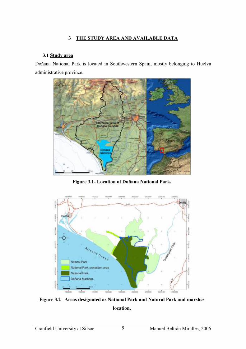
3.1 Study area
Doñana National Park is located in Southwestern Spain, mostly belonging to Huelva
administrative province.
Figure 3.1- Location of Doñana National Park.
Figure 3.2 –Areas designated as National Park and Natural Park and marshes
location.
Cranfield University at Silsoe Manuel Beltrán Miralles, 2006 10
Climate in the marshes is classified as subhumid Mediterranean with Atlantic influences
(Sahuquillo et al., 1991). The annual average precipitation in the area is 575 mm with
20% falling during spring, 5% during summer, 35% during autumn and 40% during
winter (García & Martín, 2005). Annual actual evapotranspiration in the area has been
estimated at 400-500 mm (Bayán, 2005).
According to the Spanish Geological Survey, the annual hydrological cycle in the
marshes generally starts in October with the filling up of the marshes as a response to
the first rains. The filling up continues progressively until the area flooded reaches its
annual maximum, between December and April. From April onwards, the area flooded
gradually decreases towards its minimum size, with small water bodies generated
artificially or by groundwater emerging in the marshes.
The hydrologic functioning of Doñana marshes has suffered from several modifications
in the last 50 years due to human activities. Therefore, the description below has been
reduced to the description of the conditions during the period of study, from 1994 until
2004.
There are three main inputs of water to Doñana marshes: direct precipitation, runoff and
groundwater. Main groundwater inputs, coming from the “Almonte-Marismas” aquifer,
emerge to the surface prior to their arrival at the marshes, flowing into them merged
with the river flow. Runoff is mainly concentrated in creeks. Until April 1998, the
catchment covered 2,562 square kilometres and the marshes also received additional
water inputs from the Guadiamar River when it was in spate. On the 25th of April 1998,
the Guadiamar River was polluted with heavy metals coming from a toxic spill and
actions were taken to prevent the pollutants getting into the National Park. Since then,
the Guadiamar River no longer contributes to Doñana’s hydrology, the catchment being
reduced to 1,071 square kilometres.

Cranfield University at Silsoe Manuel Beltrán Miralles, 2006 11
Figure 3.3– Catchments of the main runoff contributors to Doñana marshes
Main water outputs are evapotranspiration and discharge to the Guadalquivir River.
According to Casas and Urdiales (1995), the losses of water by infiltration in the
marshes can be considered negligible due to the clay texture of their soils. The
discharge to the Guadalquivir River is generally controlled by the Park managers by
means of gates that are opened at those moments with an excessive level of water.
Marsh soils in Doñana are mainly clay and clay-loam textured soils classified as
Entisols and Aridisols (Clemente et al. 1998). The catchments of El Partido Creek and
La Rocina Creek are mainly characterised by sandy soils, whereas catchments of the
Cañada Mayor Creek and the Guadiamar River are more heterogeneous, slates, marls,
granites and volcanic materials being present (lithology map included in Appendix D).

Cranfield University at Silsoe Manuel Beltrán Miralles, 2006 12
3.2 Available data
The period 1994-2004 was selected for the calibration and validation of the model due
to the large amount of meteorological data and Landsat images available at the Doñana
Biological Station for that period.
3.2.1 Flood extent data
GIS coverages representing the shape and size of the flooded area in the marshes with a
spatial resolution of 30 metres for 88 dates from the period 1994-2004 were provided by
LAST-EBD. The process by which the coverages were obtained is described by
Aragonés et al. (2005) and consisted firstly in the geometric correction, radiometric
correction and radiometric normalisation of Landsat (TM and ETM+) images. Then, the
flooded areas for each image were determined using the waveband 5 of the sensors. The
overall accuracy of the results obtained was 99%, using 204 field observations as
control points.
3.2.2 Meteorological data
Daily data from meteorological stations in the catchment for the period 1994-2004,
acquired from the Spanish Meteorological Institute by LAST-EBD, were employed.
The data acquired consisted of daily values for thirteen pluviometric and eight
thermometric stations. A more detailed description of the climate data employed is
contained in section 4.1.
3.2.3 Digital Elevation Models
A Digital Elevation Model (DEM) of the Doñana marshes obtained using LIDAR
technology in September 2002 was employed. The DEM had a vertical spatial
resolution of 1 centimetre and a horizontal spatial resolution of 2 metres, and it was
provided by LAST-EBD.
A DEM of the catchment with vertical spatial resolution of 10 centimetres and
horizontal spatial resolution of 10 metres was obtained from the DEM of Andalusia
“MDT 10x10 de Andalucía, vuelo 2001-2002” (Junta de Andalucía, 2002), provided by
LAST-EBD. The DEM had been developed by the Andalusian Government from aerial
Cranfield University at Silsoe Manuel Beltrán Miralles, 2006 13
photographs at 1:5,000 scale taken during the years 2001 and 2002. A figure showing
the variations in the relief of the catchment is included in Appendix C.
3.2.4 Watercourses coverage
A GIS coverage representing the network of watercourses in the area in 2004 at
1:100,000 scale was provided by LAST-EBD (Junta de Andalucía, 2004).
3.2.5 Catchment area
The catchment was manually delimited with ArcGIS using the catchment DEM and the
watercourses coverage for the area. The catchment prior to 25th April 1998 and the
catchment after that date were delineated.
3.2.6 Lithology maps
The MAGNA series of geologic maps for the area, at 1:50,000 scale, developed by the
Spanish Geological Survey (IGME) in 1972, were obtained as scanned maps in JPEG
format from the IGME web page. These pictures were georeferenced and vectorised,
creating a vector geologic map in shapefile format. The different soil classes were then
merged according to their lithology, and a lithology map for the catchment in shapefile
format was obtained. (Appendix D).
3.2.7 Land Use/ Land Cover map.
A Land Use/Land Cover map for the area, at 1:50,000 scale, was obtained from the
digital map “Usos y coberturas vegetales del suelo, 1999” (Junta de Andalucía, 1999),
created for Andalusia using photointerpretation of Landsat and IRS images and aerial
photographs taken during July 1999. (Land Use/ Land Cover map for the area included
in Appendix E)

Cranfield University at Silsoe Manuel Beltrán Miralles, 2006 14

Cranfield University at Silsoe Manuel Beltrán Miralles, 2006 15
4 METHODOLOGY
The model developed was based in a water balance, in which the variation in the
volume of water in the marshes between two different dates can be explained using
equation (1):
∑ ∑= =
−=−y
xi
y
xi
iixy OIVV (1)
where:
- yV : Water volume on the day y
- xV : Water volume on the day x
- ∑=
y
xi
iI : Sum of water inputs between days x and y
- ∑=
y
xi
iO : Sum of water outputs between days x and y
The inputs considered for the study were precipitation and runoff. The only output
considered was evaporation, infiltration losses and discharges to the Guadalquivir River
not being included in the balance. Equation (1) turns then into equation (2).
∑∑∑===
−+=−y
xi
i
y
xi
i
y
xi
ixy ERPVV (2)
where:
- ∑=
y
xi
iP : Accumulated precipitation directly falling on the marshes between days
x and y.
- ∑=
y
xi
iR : Accumulated runoff reaching the marshes between days x and y.
- ∑=
y
xi
iE : Accumulated evaporation from the marshes between days x and y.
Knowing the daily inputs and outputs of water throughout the whole hydrologic year
and establishing an initial volume, the volume of water contained in the marshes for
each day of the hydrologic year can therefore be simulated (table 4.1). The initial day of

Cranfield University at Silsoe Manuel Beltrán Miralles, 2006 16
the model was set as the 1st of September, date that has been considered in this study as
the initial day of the hydrologic year due to practical reasons. The initial volume of
water at the beginning of the hydrologic year was considered negative: marsh soils are
dry after the summer and the first amounts of water reaching the marshes will be
absorbed, not causing an increase in the flood extent. The amount of water absorbed by
the marsh soils between two images was introduced in the balance by means of the
variable Abs. It was assumed that soil dryness at the beginning of the hydrologic year
would be maximum. Therefore, the initial volume of water the first of September was
then defined by the value Absmax, which stands for the maximum amount of water the
marshes’ soils can absorb at the beginning of the hydrologic year.
Table 4.1- Daily water balance used to simulate the variation in
the volume of water contained in the marshes throughout the
hydrologic year.
Date Day Volume
1st September 0
maxAbsVo −=
2nd September 1
max1111 AbsERPV −−+=
3rd September 2
12222 VERPV +−+=
……………… ……… ..............................................
i 1−+−+= iiiii VERPV
Discharges to the Guadalquivir River limit the water volume the marshes can contain. A
maximum volume of 85,584,608 cubic metres (Vmax) was considered for the model
(maximum volume of water contained in the marshes during the period 1994-2004,
calculated from the satellite images). If the volume calculated by the balance for the day
i was higher than Vmax,, then Vi was given the value 85,584,608 m3, this also being the
value of Vi used for the calculation of Vi+1. For the calibration and validation of the
models, the volume simulated was considered zero for those days with negative V.
In this way, it was possible to calculate the volume of water contained in the marshes
for each day of the hydrologic year (calculations included in Appendix K). At the same
Cranfield University at Silsoe Manuel Beltrán Miralles, 2006 17
time, an expression relating flood extent to water volume was empirically obtained (see
section 4.2) and hence the variation in the flood extent throughout the hydrologic year
was calculated.
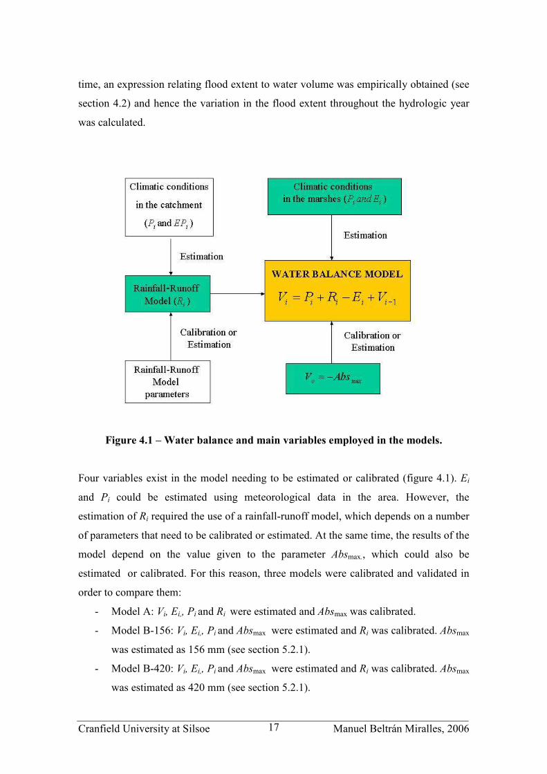
Figure 4.1 – Water balance and main variables employed in the models.
Four variables exist in the model needing to be estimated or calibrated (figure 4.1). Ei
and Pi could be estimated using meteorological data in the area. However, the
estimation of Ri required the use of a rainfall-runoff model, which depends on a number
of parameters that need to be calibrated or estimated. At the same time, the results of the
model depend on the value given to the parameter Absmax., which could also be
estimated or calibrated. For this reason, three models were calibrated and validated in
order to compare them:
- Model A: Vi, Ei,, Pi and Ri were estimated and Absmax was calibrated.
- Model B-156: Vi, Ei,, Pi and Absmax were estimated and Ri was calibrated. Absmax
was estimated as 156 mm (see section 5.2.1).
- Model B-420: Vi, Ei,, Pi and Absmax were estimated and Ri was calibrated. Absmax
was estimated as 420 mm (see section 5.2.1).

Cranfield University at Silsoe Manuel Beltrán Miralles, 2006 18
Two additional models were developed to be used as controls. In both models, runoff
was considered null and all variables were estimated, calibration not being required.
- Model C-156: Absmax estimated equal to 156 mm.
- Model C-420: Absmax estimated equal to 420 mm.
The area considered as marshes in the study was 354,812,630 m2, larger than the
marshes contained within the National Park, it including other surrounding areas that
flood naturally (figure 4.2)
Figure 4. 2 – Area considered as marshes in the study and areas flooded during the
hydrologic year 2002-2003
The steps conducted prior to the calibration were:
1. Infilling of climate data gaps.
2. Calculation of the relationship “water volume-flood extent”.
3. Estimation of direct rainfall falling on the marshes.
4. Estimation of the evaporation from the marshes.

Cranfield University at Silsoe Manuel Beltrán Miralles, 2006 19
5. Calculation of the time of concentration.
6. Calculation of Absmax (only required for model B).
7. Estimation of Témez model inputs.
8. Distribution of data for calibration and validation.
4.1 Infilling of climate data gaps.
As a first step, data from thirteen pluviometric and eight thermometric stations were
acquired. As the degree of data completeness of many of these stations was rather low,
six pluviometric and three thermometric stations were finally selected (figure 4.3). Data
completeness was the main criterion employed in the final selection, but differences in
altitude and location of the stations were also considered. The other stations were used
to infill data gaps of the stations selected (see Appendix F for a detailed description of
the process conducted).
Figure 4.3 – Location, altitude and code of the meteorological stations employed.

Cranfield University at Silsoe Manuel Beltrán Miralles, 2006 20
4.2 Water volume calculation
The volume of water contained in the marshes was calculated for 87 of the 88 dates with
satellite data providing the flood extension and shape obtained from satellite images
(table 4.2). For this purpose, the DEM of the marshes and the flood extent coverage
files were used. Each image contained different water bodies that form the marshes. The
average water surface level of each of the water bodies was obtained by calculating the
average altitude of the pixels in the perimeter of the water body. The DEM and the GIS
coverage of the date were combined for this purpose. Each pixel flooded was assigned
the average water surface level of the water body it belonged to, and the depth of the
water was then calculated subtracting the level of each pixel in the DEM. The volume of
water contained in each pixel was obtained by considering the pixel surface of 900 m2,
and these volumes were added to obtain the total amount of water in the marshes for
that date. This way, the volumes of water in the marshes for the 87 dates were obtained.
Table 4. 2 - Dates for which the volume was calculated from satellite images.
The number contained in each cell indicates the day the image was taken for
a certain month (columns) and year (row).
Jan Feb Mar Apr May June July Aug Sept Oct Nov Dec1994 6 25 11
1995 12 2 18 20 21 23 24 9
1996 3 22 23 9 10 26 27 30
1997 18 6 9 26 12 28 13 29 16 17
1998 9 25 13 15 16 3 19 6 22
1999 7 8 13 31 16 27 12 7 23
2000 18 3 19 2 12 13 6 22 8 1
2001 20 21 10 28 13 29
2002 7 24 29 31 16 2 18 3 19 22 7
2003 10 11 16 18 27 13 14 12
2004 21 25 26 13 15
An equation estimating the extension of the area flooded (S) as a function of the volume
of water contained in the marshes (V) was necessary for the model. Due to the
geometric relationship between volume and surface, it was assumed that a linear
relationship should exist between V1/3
and S1/2,
, hence between V and S3/2. A third

Cranfield University at Silsoe Manuel Beltrán Miralles, 2006 21
degree polynomial function was fitted and compared with the linear relationship in
order to determine which provided the best results. (Data employed included in
Appendix K)
4.3 Direct rainfall calculation
The amount of rainfall falling directly on the marshes was calculated using daily data
from the meteorological station closest to the marshes (station 5858, “Almonte-
Doñana”). The conversion from mm of rainfall to water volume was carried out
considering a constant catchment area equal to the size of the marshes.
4.4 Evaporation calculation
Daily evaporation was calculated as the reference evapotranspiration (ETo, estimated
with the Hargreaves equation) multiplied by 1.05, which is the Kc coefficient for open
water with less than 2 metres depth suggested in the FAO Irrigation and Drainage Paper
No.56 (Allen et al., 1998). Evaporation in mm was multiplied by the daily flood extent
to obtain evaporation expressed in volume. Daily flood extent was estimated from the
daily water volume calculated by the balance using the equation S = f (V) explained in
section 4.2 (see section 6.1 for the equation).
4.5 Time of concentration calculation
The time of concentration was calculated for the main surface water contributors to the
marshes. The calculation was carried out using the equation calibrated by Kirpich
(1940):
385.077.00078.0 −⋅⋅⋅= SLCtc (3)
where:
- tc: time of concentration in minutes
- C: coefficient whose value varies depending on the characteristics of the flow
- L: maximum length of the channel in feet
- S: average slope of the catchment in feet/feet.
Parameter C is set to a value lower than 1 for flows in concrete surfaces or channels.
This not being the case of the Doñana’s rivers and creeks, C value was set to 1. L and S

Cranfield University at Silsoe Manuel Beltrán Miralles, 2006 22
for each contributor were calculated by means of the watercourses coverage and the
DEM respectively (see Appendix G).
4.6 Absmax calculation
Absmax was estimated as:
)()()( 2
maxmax mAreammSlAbs ⋅= (4)
where Smax is the maximum moisture storage capacity of the marshes’ soils, which was
calculated using equation (5)
)()()(max mmdepthmmS rs ⋅−= θθ (5)
where θs stands for the saturated water content and θr for the residual water content,
both expressed in cm3 water/cm
3 soil.
The data necessary to calculate the different parameters were obtained from Doñana
soils analyses published by Clemente et al. (1998). Texture data of different soil profiles
was introduced in the Rosetta software (Schaap et al., 2001) developed by the United
States Salinity Laboratory, which returned the θr and θs for its different horizons. Then,
knowing the depth of each horizon, the Smax for each of them was calculated. The
published data indicated the depth of the water table at the end of the dry season for the
soil profiles employed. Smax for each profile was calculated as the sum of the Smax of the
horizons located above the water table. (Appendix H)
4.7 Estimation of Témez model inputs.
A single value for daily precipitation and daily reference evapotranspiration in the
whole catchment (inputs to the Témez model) were obtained from the different stations
through the use of Thiessen polygons (results included in tables 4.3 and 4.4,
calculations in Appendix I). Daily reference evapotranspiration was estimated using the
Hargreaves equation and it was used as input to the model.

Cranfield University at Silsoe Manuel Beltrán Miralles, 2006 23
Table 4.3 - Meteorological stations and Thiessen coefficients obtained for the
catchment existing before 25th April 1998.
Precipitation Evapotranspiration
Station Thiessen coefficient Station Thiessen coefficient
4622 0.1576 4609F 0.1175
4628 0.1072 5835E 0.5142
5822 0.2393 5858 0.3683
5826 0.0980
5843 0.2931
5858 0.1048
Table 4.4 - Meteorological stations and Thiessen coefficients for the catchment
existing after 25th April 1998.
Precipitation Evapotranspiration
Station Thiessen coefficient Station Thiessen coefficient
4622 0.3579 4609F 0
4628 0.2563 5835E 0.1073
5822 0 5858 0.8927
5826 0
5843 0.1353
5858 0.2505
The initial conditions of the Témez model (Bo and So,) were both established as 0.01
mm. Daily reference evapotranspiration was estimated using the Hargreaves equation
and used as input to the Témez model. The conversion of runoff from millimetres to
cubic metres took into account the change in the catchment area which occurred after
the 25th of April 1998. The catchment sizes were calculated using ArcGIS:
- Before 25/04/1998: 2,562,375,072 m2
- After 25/04/1998: 1,071,852,914 m2

Cranfield University at Silsoe Manuel Beltrán Miralles, 2006 24
4.8 Data distribution for calibration and validation
The ten hydrologic years available (from 1994-1995 to 2003-2004) were sorted out into
two sets: calibration and validation, each containing five years. Accumulated reference
evapotranspiration and rainfall values during each year were previously analysed. Little
variation was observed in accumulated evapotranspiration values, precipitation being
the key element considered for the allocation of the hydrologic years. At the same time,
each set should include years before and after April 1998. The ten years were allocated
as indicated in table 4.5
Table 4.5 –Precipitation of each hydrologic year and set to which it was assigned (calibration or validation).
Hydrologic year Precipitation
(mm) Set 1994-1995 253 Calibration
1995-1996 1,032 Calibration
1996-1997 885 Validation
1997-1998 722 Calibration
1998-1999 253 Validation
1999-2000 514 Calibration
2000-2001 681 Validation
2001-2002 582 Calibration
2002-2003 550 Validation
2003-2004 775 Validation

Cranfield University at Silsoe Manuel Beltrán Miralles, 2006 25
5 CALIBRATION
There were two variables of the water balance model that needed to be calibrated: Ri
and Absmax. Both variables could not be calibrated at the same time, so it was required to
estimate one of them in order to calibrate the other. Absmax was the variable calibrated
for model A, whereas runoff was the variable calibrated for models B. Not only the
variables calibrated but also the approaches employed for the calibration were different
and are described in this chapter.
5.1 Model A calibration
The Témez model parameters were estimated using the values obtained by Verdú
(2004), who calibrated the Témez model for the Meca River catchment using runoff
records of the river. The Meca River is located in Southwestern Spain and it is
contained in the same political region as Doñana (figure 5.1). Therefore, it was assumed
that the parameters calibrated for this river might be applicable to Doñana catchment, an
assumption that will be tested with the validation of the model.
Figure 5.1 –Location of the Meca River and Doñana.

Cranfield University at Silsoe Manuel Beltrán Miralles, 2006 26
The work of Verdú provides different parameter values depending on the calibration
criterion employed (“events”, “peak flow criterion” or “all data”). The set of values
selected was that obtained when calibrating against “all data” (table 5.1).
Table 5.1 – Values of Témez parameters calibrated for the Meca River
by Verdú (2004).
Parameter Value Description
Smax 122 Maximum soil moisture storage capacity (mm)
Imax 190 Maximum infiltration (mm)
α 0.95 Aquifer discharge parameter (day-1)
c 0.6 Surplus parameter
Témez model was run employing these values and the daily precipitation and reference
evapotranspiration in the catchment. Daily runoff values were then obtained and
introduced into the water balance model in order to calibrate the variable Absmax.
The value given to Absmax determines the moment when the marshes start flooding. This
process happens in a short time lapse, generally in less than the 16 days between two
consecutive Landsat images. The Absmax value returned was the one that fulfilled the
following requirements:
- The flooding simulated started in the interval indicated by the satellite images;
and
- The R2 of the correlation between the simulated (calculated by the model) and
observed (calculated from the satellite images) flood extents was maximum.
The Absmax value returned from the calibration was 156 mm, with a R2 equal to 0.8193
(p<0.05).

Cranfield University at Silsoe Manuel Beltrán Miralles, 2006 27
0.0E+00
5.0E+07
1.0E+08
1.5E+08
2.0E+08
2.5E+08
3.0E+08
3.5E+08
0.0E+00 5.0E+07 1.0E+08 1.5E+08 2.0E+08 2.5E+08 3.0E+08
Observed area (m2)
Sim
ulated area (m
2 )
Figure 5.2 – Correlation between observed and simulated flood extents obtained
from the calibration of model A.
-1.8E+08
-1.6E+08
-1.4E+08
-1.2E+08
-1.0E+08
-8.0E+07
-6.0E+07
-4.0E+07
-2.0E+07
0.0E+00
2.0E+07
0.0E+00 5.0E+07 1.0E+08 1.5E+08 2.0E+08 2.5E+08 3.0E+08
Simulated area ( m2)
Residual (m
2 )
Figure 5.3 – Distribution of the residuals obtained from the calibration of model A.

Cranfield University at Silsoe Manuel Beltrán Miralles, 2006 28
5.2 Models B calibration
Taking a period of sixteen days between two consecutive Landsat images as an example
to explain the calibration approach followed.
∑∑∑===
−+=−16
1
16
1
16
1 i
i
i
i
i
ifo ERPVV (1)
From the balance (1), it is possible to calculate the accumulated runoff that explains the
variation in the volume of water in the marshes for the time between the two images
(Rrequired, or Rr):
∑∑∑===
+−−==16
1
16
1
16
1 i
i
i
ifo
i
ir EPVVRR (2)
with Vo and Vf determined from the satellite images and ∑=
16
1i
iP and∑=
16
1i
iE estimated
from meteorological data. Rr can be calculated for several sequences between Landsat
images, and the Témez model parameters can be then calibrated adjusting the
accumulated runoff simulated for the sequences to the Rr values calculated for them.
The calculations conducted during the calibration are included in Appendix K.
Three constraints limit the periods of data that can be used for the model calibration:
1. The conversion from mm to volume requires the multiplication by the area in
which each process occurs. The area is constant and equal to the size of the
marshes for precipitation. In contrast, the evaporation process depends on the
area of the marshes flooded at a moment, which is only known for the initial
and final day of the sequence. It is necessary then to estimate the flood extent
for each day. It was supposed that the flood extent increased linearly between
two pictures. This not being real, it is necessary to use short time lapses for the
calibration in order to reduce the errors associated with the process.
2. The values for the initial conditions of the Témez model (So and Bo) are
unknown but, if the initial date is set to a dry moment, they can be estimated as
close to zero. Setting the initial image in a dry period makes necessary the
introduction of the Absmax variable in the expression (2):

Cranfield University at Silsoe Manuel Beltrán Miralles, 2006 29
max
16
1
16
1
16
1
AbsEPVVRRi
i
i
ifo
i
ir ++−−== ∑∑∑===
(3)
3. When the amount of water in the marshes reaches a certain level, discharges to
the Guadalquivir River occur and balance (3) will not be fulfilled. Hence, the
final image cannot be a situation of maximum flood. However, it must be
flooded to a large extent, as the soils must have absorbed enough water to
consider the absorption as maximum (Absmax). Otherwise, the amount of water
absorbed will be lower than Absmax and unknown.
These restrictions reduce considerably the number of satellite image intervals that can
be employed for the calibration process. Only 7 sequences, using 14 satellite images,
fulfilled these requirements (table 5.2).
Table 5.2 – Sequences employed for the calibration of models B-156 and B-420.
Sequence Initial Date
Final Date
V initial (m3)
V final (m3)
S initial (m2)
S final (m2)
1 06/09/1994 25/11/1994 54,389 679,399 1,130,400 5,450,400
2 27/09/1996 30/11/1996 516,781 1,997,866 3,563,252 22,542,396
3 16/10/1997 17/11/1997 393,691 12,188,929 3,142,800 77,831,102
4 22/12/1998 08/02/1999 475,387 1,237,145 4,359,600 12,852,000
5 12/09/1999 07/11/1999 89,706 15,021,307 1,111,188 121,602,597
6 29/06/2001 07/01/2002 4,317,815 31,012,908 37,952,099 175,188,597
7 07/11/2002 10/01/2003 667,372 52,915,496 6,258,600 227,647,794
The process followed was:
1. Selection of a value for Absmax.
2. Calculation of the most–likely values for Témez parameters.
3. Calibration and sensitivity analysis.
4. Final parameter values selection
5.2.1 Absmax calculation
Model B required the estimation of Absmax , which was given two different values:
- Model B-156. The model was calibrated assuming Absmax equal to 156 mm, the
value obtained from the calibration of model A.
Cranfield University at Silsoe Manuel Beltrán Miralles, 2006 30
- Model B-420. The model was calibrated setting Absmax equal to the value
calculated from the published data on the marshes’ soils: 420 mm. Although the
Smax of the different soils varied between 265 and 566 mm, these were extreme
values and not too frequent. The calculated value for the most common soils in
the marshes (Salorthids and Aeric Fluvaquents; Clemente et al., 1998) varied
between 374 and 446 mm. The average of the values obtained for the most
frequent soils was 420mm, and it was the value selected for model B-420.
(Calculation included in Appendix H).
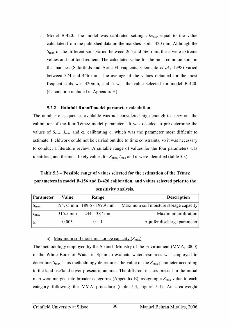
5.2.2 Rainfall-Runoff model parameter calculation
The number of sequences available was not considered high enough to carry out the
calibration of the four Témez model parameters. It was decided to pre-determine the
values of Smax, Imax and α, calibrating c, which was the parameter most difficult to
estimate. Fieldwork could not be carried out due to time constraints, so it was necessary
to conduct a literature review. A suitable range of values for the four parameters was
identified, and the most likely values for Smax, Imax and α were identified (table 5.3).
Table 5.3 – Possible range of values selected for the estimation of the Témez
parameters in model B-156 and B-420 calibration, and values selected prior to the
sensitivity analysis.
Parameter Value Range Description
Smax 194.75 mm 189.6 - 199.9 mm Maximum soil moisture storage capacity
Imax 315.5 mm 244 – 387 mm Maximum infiltration
α 0.003 0 – 1 Aquifer discharge parameter
a) Maximum soil moisture storage capacity (Smax)
The methodology employed by the Spanish Ministry of the Environment (MMA, 2000)
in the White Book of Water in Spain to evaluate water resources was employed to
determine Smax. This methodology determines the value of the Smax parameter according
to the land use/land cover present in an area. The different classes present in the initial
map were merged into broader categories (Appendix E), assigning a Smax value to each
category following the MMA procedure (table 5.4, figure 5.4). An area-weight

Cranfield University at Silsoe Manuel Beltrán Miralles, 2006 31
adjustment was used to determine the overall value for the parameter in the catchment
before and after April 1998 (table 5.5). The average value of 194.75 mm was used in the
model.
Table 5.4 – Value of Smax assigned to each land use
present in the catchment.
Landcover/Landuse Smax (mm)
Artificial surfaces 40
Areas with sparse vegetation 100
Unirrigated land 155
Irrigated land 210
Pasture land 150
Heterogeneous agronomic fields 195
Permanent crops 210
Scrub 135
Woodland 225
Wetlands 300
Figure 5.4- Maximum soil moisture storage capacity (mm) in the catchment.

Cranfield University at Silsoe Manuel Beltrán Miralles, 2006 32
Table 5.5 – Smax values estimated for the catchment.
Before 25/04/1998 After 25/04/1998 Average
Smax (mm) 199.9 189.6 194.75
b) Maximum infiltration capacity (Imax)
Imax was also determined employing the methodology used by the Spanish Ministry of
the Environment (MMA, 2000) in the White Book of Water in Spain. This methodology
determines the value of Imax according to lithology. A value for Imax was assigned to
each lithology class present in the area following the values described by the MMA
(2000). (table 5.6).
Imax for the catchment was then obtained (figure 5.5) using an area-weight adjustment
for the catchment prior to April 1998 and after April 1998 (table 5.7). The average value
of 315.5 mm was selected for the model
Table 5.7 – Imax values estimated for the catchment.
Before 25/04/1998 After 25/04/1998 Average
Imax (mm) 244 387 315.5
Table 5.6 – Values of Imax assigned to
each lithology class present in the area.
Lithology Imax (mm)
Sands 450
Marls 85
Slate 40
Alluvium 400
Volcanic materials 275
Granites 65
Clastic Limestones 250

Cranfield University at Silsoe Manuel Beltrán Miralles, 2006 33
Figure 5.5 - Maximum infiltration capacity (mm) in the catchment.
c) Aquifer discharge parameter (α)
The range of values of the aquifer discharge parameter for the area was identified from
the White Book of Water in Spain (MMA, 2000). This work calculates the aquifer
discharge parameter according to the lithology in the area, the α provided for the
Almonte-Marismas being included within the range 0.001 - 0.005 day-1. An
intermediate value of 0.003 day-1 was selected.
5.2.3 Calibration and sensitivity analysis.
The criterion employed for the calibration was to minimise the sum of the square of the
residuals (Rrequired - Rsimulated). Models B-156 and B-420 were calibrated, obtaining
different parameter values.
For each model, the same methodology was conducted; firstly, Smax, Imax and α were set
to the values calculated in section 5.2.2. A c value was then calibrated. Establishing this
value as fixed, a sensitivity analysis of the other parameters was carried out. The
sensitivity analysis indicated α as the most influential parameter, and thus its value was
modified between 0 and 1 to obtain the best results. Smax and Imax were calculated as the

Cranfield University at Silsoe Manuel Beltrán Miralles, 2006 34
average of two situations (before and after 25th of April 1998). Therefore, the
modification of these values would, theoretically, provide better results for one situation
and worse for other. For this reason, Smax and Imax were not included in the sensitivity
analysis.
5.2.4 Final parameter values selected
The values obtained from the calibration process and employed for the validation of the
models are described in table 5.8.
Table 5. 8 – Values of Absmax and Témez parameters
employed in the calibration of models B-156 and B-420
and sum of squares of the residuals obtained.
Variable Model B-156 Model B-420
Absmax (mm) 156 420
Smax (mm) 194.75 194.75
Imax (mm) 315.5 315.5
α (day-1) 0.03 0.99
c 0.99 0.01
Sum of squares of
the residuals (mm2)
641 12,796

Cranfield University at Silsoe Manuel Beltrán Miralles, 2006 35
6 RESULTS
6.1 Relationship “flood extent-water volume”
A linear regression to observed data was fitted, obtaining the equation (1):
2/351060601.1 SV ⋅⋅= − ; R2 = 0.9839 (1)
V expressed in m3 and S in m
2.
V was determined from S data and therefore V should not be treated as an independent
variable in the regression. For this reason, a linear regression considering S = f (V2/3)
was not directly obtained and the equation estimating S as a function of V was obtained
as the inverse of equation (1):
3/297.1570 VS ⋅= ; R2 = 0.9839 (2)
V expressed in m3 and S in m
2.
0.E+00
1.E+07
2.E+07
3.E+07
4.E+07
5.E+07
6.E+07
7.E+07
8.E+07
9.E+07
1.E+08
0.0E+00 7.0E+11 1.4E+12 2.1E+12 2.8E+12 3.5E+12 4.2E+12 4.9E+12
(Surface (m2))3/2
Volume (m3 )
Figure 6.1 – Linear function showing the relationship between S3/2 and V from
which the function S=f (V2/3) was derived.
A 3rd degree polynomial regression S = f (V) was also fitted to the data:
VVVS ⋅+⋅⋅−⋅⋅= −− 1358664.9103440526.1108761431.7 27316 ; R2 = 0.9958 (3)

Cranfield University at Silsoe Manuel Beltrán Miralles, 2006 36
0.0E+00
4.0E+07
8.0E+07
1.2E+08
1.6E+08
2.0E+08
2.4E+08
2.8E+08
3.2E+08
0.0E+00 1.0E+07 2.0E+07 3.0E+07 4.0E+07 5.0E+07 6.0E+07 7.0E+07 8.0E+07 9.0E+07
Volume (m3)
Area (m
2 )
Figure 6.2 – Third degree polynomial function showing the extension of the area
flooded in the marshes in function of the volume of water contained by them.
In this case, V was used as independent variable due to the difficulty of obtaining the
inverse of the polynomial function V= f (S)
The distribution of the residuals for both equations was analysed (figure 6.3). Whereas
the distribution of the residuals of the polynomial function showed no clear pattern, the
linear function was clearly biased, underestimating surfaces corresponding to
intermediate volume values and overestimating those corresponding to high volumes.
The reason is that the marshes, not being a perfect geometric model, would not
necessarily follow a linear relationship between surface and volume. Hence, the
polynomial equation was utilised due to its higher R2 value and its unbiased residuals
distribution of errors.

Cranfield University at Silsoe Manuel Beltrán Miralles, 2006 37
-4.E+07
-3.E+07
-2.E+07
-1.E+07
0.E+00
1.E+07
2.E+07
3.E+07
4.E+07
0.E+00 1.E+07 2.E+07 3.E+07 4.E+07 5.E+07 6.E+07 7.E+07 8.E+07 9.E+07
Volume (m3)
Residuals (m
2 )Linear function Polynomial function
Figure 6.3 – Distribution of the residuals of the linear and polynomial functions.
6.2 Time of concentration
The times of concentration calculated for the main water contributors to the marshes
and the data used for its calculation are included in table 6.1. See Appendix G for visual
identification of the watercourses employed in the calculation.
Table 6.1 – Data used in the calculation of the time of concentration of the main
watercourses using Kirpich equation.
Watercourse L(m) H(m) L(feet) H(feet) C Tc min Tc (days) Guadiamar
River 126,351.2 502.9 414,538.2 1650.0 1.0 1385.6 0.96 Cañada Mayor Creek 78,473.8 173.0 257,460.0 567.6 1.0 1205.5 0.84
El Partido Creek 33,068.8 127.8 108,493.3 419.3 1.0 499.2 0.35
La Rocina Creek 35,996.0 70.5 118,097.1 231.3 1.0 692.3 0.48
The results obtained for the time of concentration are, in every case, lower than one day.
Therefore, it can be assumed that the runoff reaching the marshes in one day was
generated by the meteorological conditions of the same day, no modification in the
water balance being required.

Cranfield University at Silsoe Manuel Beltrán Miralles, 2006 38
6.3 Models validation
The models were validated against the flood extent calculated from the satellite images
for the hydrologic years 1996-1997, 1998-1999, 2000-2001, 2002-2003 and 2003-2004.
The final dates of the sequences used for the calibration of model B and included in
these years were excluded from the validation data. The different models were assessed
using as criteria:
- Coefficient of determination (R2) of the correlation between the simulated and
the observed flood extent.
- Visual analysis of the distribution of the residuals.
- a and b from the correlation:
o )()( 22 mSbamS simulatedobserved ⋅+=
- Weighted R2 (w R
2), as defined in section 2.4.
The figures displayed in this chapter show the correlations and the residuals plot of each
model. The figures showing the daily flood extent simulated by each model for the
validation period have been included in the Appendix J due to the large number of
graphs produced.

Cranfield University at Silsoe Manuel Beltrán Miralles, 2006 39
6.3.1 Model A
0.0E+00
5.0E+07
1.0E+08
1.5E+08
2.0E+08
2.5E+08
3.0E+08
3.5E+08
0.0E+00 5.0E+07 1.0E+08 1.5E+08 2.0E+08 2.5E+08 3.0E+08
Observed area (m2)
Sim
ulated area (m
2 )
Figure 6.4 - Correlation obtained from model A validation.
-2.0E+08
-1.6E+08
-1.2E+08
-8.0E+07
-4.0E+07
0.0E+00
4.0E+07
8.0E+07
1.2E+08
1.6E+08
2.0E+08
2.4E+08
0.0E+00 5.0E+07 1.0E+08 1.5E+08 2.0E+08 2.5E+08 3.0E+08
Simulated area (m2)
Residual (m
2)
Figure 6.5 - Residual plot obtained from the validation of model A.
Table 6.2 – Results from model A validation.
Equation 7459982)(912613.0)( 22 −⋅= mSmS simulatedobserved
R2 (probability) 0.96 (<0.05)
w R2 0.88

Cranfield University at Silsoe Manuel Beltrán Miralles, 2006 40
6.3.2 Model B-156
0.0E+00
5.0E+07
1.0E+08
1.5E+08
2.0E+08
2.5E+08
3.0E+08
3.5E+08
0.0E+00 5.0E+07 1.0E+08 1.5E+08 2.0E+08 2.5E+08 3.0E+08
Observed area (m2)
Simulated area (m
2 )
Figure 6.6 - Correlation obtained from model B-156 validation.
-2.0E+08
-1.6E+08
-1.2E+08
-8.0E+07
-4.0E+07
0.0E+00
4.0E+07
8.0E+07
1.2E+08
1.6E+08
2.0E+08
2.4E+08
0.0E+00 5.0E+07 1.0E+08 1.5E+08 2.0E+08 2.5E+08 3.0E+08
Simulated area (m2)
Residual (m
2)
Figure 6.7 - Residual plot obtained from the validation of model B-156.
Table 6.3 – Results from model B-156 validation.
Equation 16163224)(768840.0)( 22 −⋅= mSmS simulatedobserved
R2 (probability) 0.82 (<0.05)
w R2 0.63
Cranfield University at Silsoe Manuel Beltrán Miralles, 2006 41
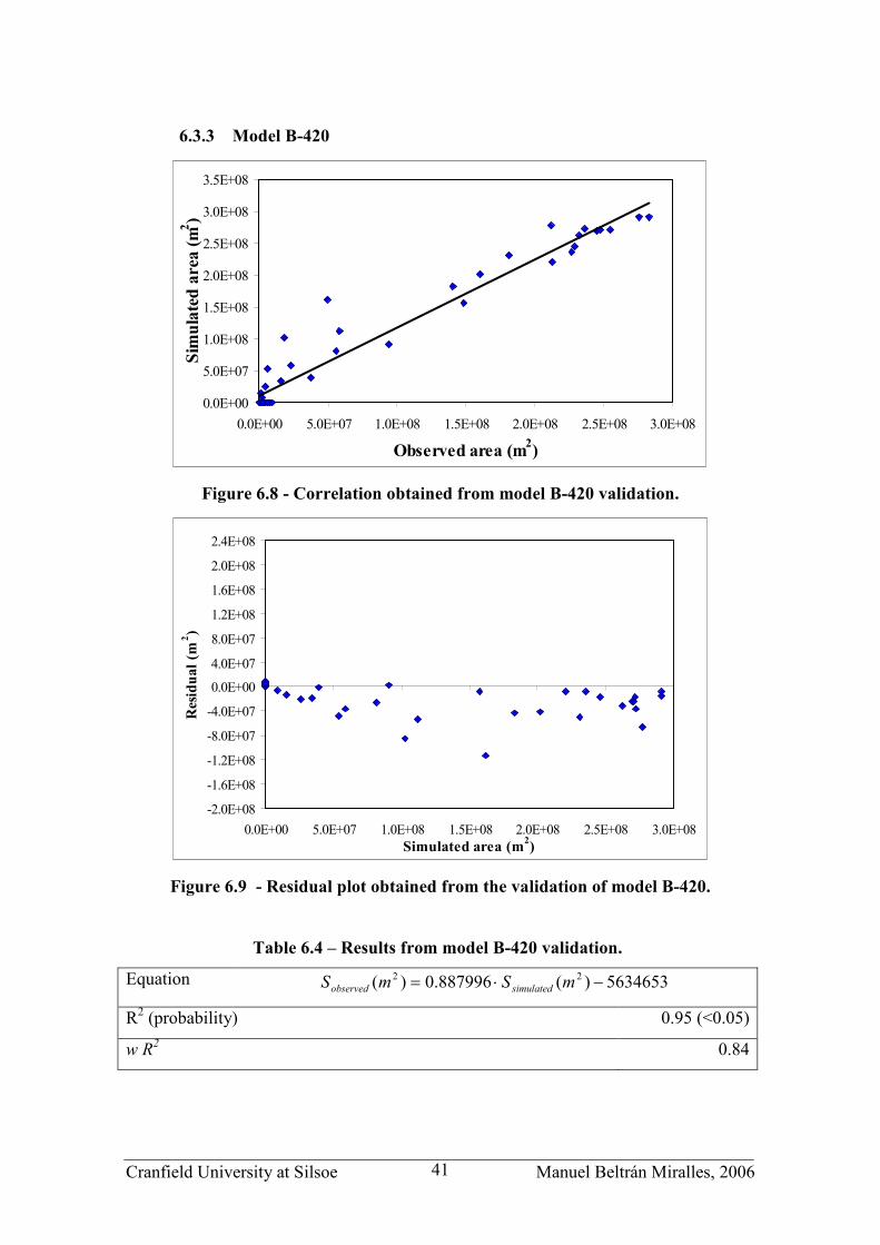
6.3.3 Model B-420
0.0E+00
5.0E+07
1.0E+08
1.5E+08
2.0E+08
2.5E+08
3.0E+08
3.5E+08
0.0E+00 5.0E+07 1.0E+08 1.5E+08 2.0E+08 2.5E+08 3.0E+08
Observed area (m2)
Sim
ulated area (m
2 )
Figure 6.8 - Correlation obtained from model B-420 validation.
-2.0E+08
-1.6E+08
-1.2E+08
-8.0E+07
-4.0E+07
0.0E+00
4.0E+07
8.0E+07
1.2E+08
1.6E+08
2.0E+08
2.4E+08
0.0E+00 5.0E+07 1.0E+08 1.5E+08 2.0E+08 2.5E+08 3.0E+08
Simulated area (m2)
Residual (m
2)
Figure 6.9 - Residual plot obtained from the validation of model B-420.
Table 6.4 – Results from model B-420 validation.
Equation 5634653)(887996.0)( 22 −⋅= mSmS simulatedobserved
R2 (probability) 0.95 (<0.05)
w R2 0.84

Cranfield University at Silsoe Manuel Beltrán Miralles, 2006 42
6.3.4 Model C-156
0.0E+00
5.0E+07
1.0E+08
1.5E+08
2.0E+08
2.5E+08
3.0E+08
3.5E+08
0.0E+00 5.0E+07 1.0E+08 1.5E+08 2.0E+08 2.5E+08 3.0E+08
Observed area (m2)
Sim
ulated area (m
2 )
Figure 6.10 - Correlation obtained from model C-156 validation.
-2.0E+08
-1.6E+08
-1.2E+08
-8.0E+07
-4.0E+07
0.0E+00
4.0E+07
8.0E+07
1.2E+08
1.6E+08
2.0E+08
2.4E+08
0.0E+00 5.0E+07 1.0E+08 1.5E+08 2.0E+08 2.5E+08 3.0E+08
Simulated area (m2)
Residua
l (m
2 )
Figure 6.11 - Residual plot obtained from the validation of model C-156.
Table 6.5 – Results from model C-156 validation.
Equation 6766361)(93695.0)( 22 −⋅= mSmS simulatedobserved
R2 (probability) 0.97 (<0.05)
w R2 0.91

Cranfield University at Silsoe Manuel Beltrán Miralles, 2006 43
6.3.5 Model C-420
0.0E+00
5.0E+07
1.0E+08
1.5E+08
2.0E+08
2.5E+08
3.0E+08
3.5E+08
0.0E+00 5.0E+07 1.0E+08 1.5E+08 2.0E+08 2.5E+08 3.0E+08
Observed area (m2)
Sim
ulated area (m
2 )
Figure 6.12 - Correlation obtained from model C-420 validation.
-2.0E+08
-1.6E+08
-1.2E+08
-8.0E+07
-4.0E+07
0.0E+00
4.0E+07
8.0E+07
1.2E+08
1.6E+08
2.0E+08
2.4E+08
0.0E+00 5.0E+07 1.0E+08 1.5E+08 2.0E+08 2.5E+08 3.0E+08
Simulated area (m2)
Residual (m
2)
Figure 6.13 - Residual plot obtained from the validation of model C-420.
Table 6.6 – Results from model C-420 validation.
Equation 14215541)(01246.1)( 22 +⋅= mSmS simulatedobserved
R2 (probability) 0.77 (<0.05)
w R2 0.76

Cranfield University at Silsoe Manuel Beltrán Miralles, 2006 44
6.3.6 Phases of the marshes annual hydrological cycle
In order to extend the analysis conducted, the variation in the flood extent throughout
the year was sorted out into five phases according to visual interpretation of the marshes
annual hydrological cycle:
1. Dry marshes prior to the flooding, at the beginning of the hydrologic year.
2. Filling up of the marshes.
3. Maximum flood extent.
4. Drying up of the marshes.
5. Dry marshes after the flooding, at the end of the hydrologic year.
The phases were analysed following the same criteria as for the whole hydrologic cycle.
Tables 6.7 and 6.8 show the results obtained. No images were available for the phase 2,
so no analysis could be conducted and it has been excluded from the tables.
Table 6.7- Results obtained from the analysis of each of the phases of hydrological
cycle of the marshes for models A, B-156 and B-420.
Model Criteria Overall Phase 1
(n=16)
Phase 3
(n=6)
Phase 4
(n=12)
Phase 5
(n=9)
A w R2 0.88 0.01 0.33 0.84 0.95
R2 0.96* 0.12 0.40 0.89* 0.96*
b 0.91 0.06 1.2 1.06 1.01
a -7,459,982 3,714,013 - 88,259,022 -34,674,982 -19,271,923
B-156 w R2 0.63 0.01 0.14 0.67 0.44
R2 0.82* 0.12 0.18 0.68* 0.56*
b 0.77 0.06 1.25 1.02 0.78
a -16,163,224 3,715,342 -120,495,200 -83,948,027 -54,912,108
B-420 w R2 0.84 (-) 0.27 0.81 0.91
R2 0.95* (-) 0.42 0.84* 0.92*
b 0.89 (-) 0.65 1.04 0.99
a -5,634,653 (-) 63,753,367 -40,366,509 -25,370,382

Cranfield University at Silsoe Manuel Beltrán Miralles, 2006 45
Table 6.8- Results obtained from the analysis of each of the phases of hydrological
cycle of the marshes for models C-156 and C-420.
Model Criteria Overall Phase 1
(n=16)
Phase 3
(n=6)
Phase 4
(n=12)
Phase 5
(n=9)
C-156 w R2 0.91 0.01 0.73 0.87 0.97
R2 0.97* 0.12 0.91 0.91* 0.97*
b 0.94 0.06 1.25 1.04 1
a -6,766,361 3,714,013 -90,211,052 -26,628,645 -16,381,286
C-420 w R2 0.76 (-) 0.05 0.63 0.40
R2 0.77* (-) 0.29 0.72* 0.75*
b 1.01 (-) 0.16 0.87 1.88
a 14,215,541 (-) 212,851,446 35,445,359 -21,329,851
* Probability < 0.05 n= number of images available for each phase
(-) Not calculated: all Ssimulated equal to zero

Cranfield University at Silsoe Manuel Beltrán Miralles, 2006 46
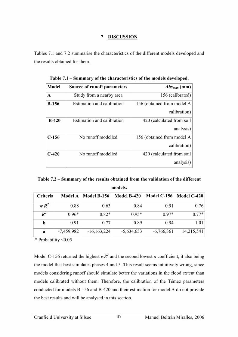
Cranfield University at Silsoe Manuel Beltrán Miralles, 2006 47
7 DISCUSSION
Tables 7.1 and 7.2 summarise the characteristics of the different models developed and
the results obtained for them.
Table 7.1 – Summary of the characteristics of the models developed.
Model Source of runoff parameters Absmax (mm)
A Study from a nearby area 156 (calibrated)
B-156 Estimation and calibration 156 (obtained from model A
calibration)
B-420 Estimation and calibration 420 (calculated from soil
analysis)
C-156 No runoff modelled 156 (obtained from model A
calibration)
C-420 No runoff modelled 420 (calculated from soil
analysis)
Table 7.2 – Summary of the results obtained from the validation of the different
models.
Criteria Model A Model B-156 Model B-420 Model C-156 Model C-420
w R2 0.88 0.63 0.84 0.91 0.76
R2 0.96* 0.82* 0.95* 0.97* 0.77*
b 0.91 0.77 0.89 0.94 1.01
a -7,459,982 -16,163,224 -5,634,653 -6,766,361 14,215,541
* Probability <0.05
Model C-156 returned the highest wR2 and the second lowest a coefficient, it also being
the model that best simulates phases 4 and 5. This result seems intuitively wrong, since
models considering runoff should simulate better the variations in the flood extent than
models calibrated without them. Therefore, the calibration of the Témez parameters
conducted for models B-156 and B-420 and their estimation for model A do not provide
the best results and will be analysed in this section.

Cranfield University at Silsoe Manuel Beltrán Miralles, 2006 48
7.1 Model A
The high wR2 obtained for model A may lead to the conclusion that Absmax can be
properly calibrated using runoff parameters from a nearby catchment. However a high
wR2 is obtained for Absmax equal to 156 mm even when daily runoff is considered null
(model C-156). Furthermore, the comparison between models B-156 and B-420 shows
that worse results have been obtained by previously calibrating Absmax with the
parameters of the Meca River catchment. Therefore, Témez parameters calibrated for
the Meca River are not applicable to Doñana catchment, and cannot be used to calibrate
Absmax. This is confirmed by the analysis of the simulated flood extents for the
hydrologic year 1998-1999, with only 253 mm of accumulated precipitation. Although
some flooding occurred in the marshes during that year, it was localised in small areas,
no important flooded areas appearing. Figure 7.1 shows the maximum flood extent
occurring during the hydrologic year 1998-1999.
Figure 7.1 – Maximum flood extent occurred during the hydrologic year 1998-1999

Cranfield University at Silsoe Manuel Beltrán Miralles, 2006 49
Figures 7.2 and 7.3 show the variation in the flood extent simulated by models B-156
and B-420 and that observed from the satellite images for the year 1998-1999.
1998-1999
0.0E+00
2.0E+07
4.0E+07
6.0E+07
8.0E+07
1.0E+08
1.2E+08
01/09/1998
21/09/1998
11/10/1998
31/10/1998
20/11/1998
10/12/1998
30/12/1998
19/01/1999
08/02/1999
28/02/1999
20/03/1999
09/04/1999
29/04/1999
19/05/1999
08/06/1999
28/06/1999
18/07/1999
07/08/1999
27/08/1999
Date
Flood
extent (m
2 )
Simulated
Observed
Figure 7.2 – Flood extents simulated by the model B-156 and observed (estimated
from the satellite images) for the hydrologic year 1998-1999.
1998-1999
0.0E+00
2.0E+07
4.0E+07
6.0E+07
8.0E+07
1.0E+08
1.2E+08
01/09/1998
21/09/1998
11/10/1998
31/10/1998
20/11/1998
10/12/1998
30/12/1998
19/01/1999
08/02/1999
28/02/1999
20/03/1999
09/04/1999
29/04/1999
19/05/1999
08/06/1999
28/06/1999
18/07/1999
07/08/1999
27/08/1999
Date
Flood
extent (m
2 )
Simulated
Observed
Figure 7.3 – Flood extents simulated by the model B-420 and observed (estimated
from the satellite images) for the hydrologic year 1998-1999.
Model B-420 simulates no flooding during the year, whereas model B-156 simulates an
important increase in the flood extent in January. This occurs because the value given to
Absmax determines the moment when the flooding occurs. These results indicate that
156mm is not a suitable value for Absmax, and corroborate that Absmax cannot be
properly calibrated using data from the Meca River.

Cranfield University at Silsoe Manuel Beltrán Miralles, 2006 50
It may be possible to use parameters calibrated for other catchments and obtain accurate
results. However, the process entails many difficulties, since parameters such as α do
not only depend on physical properties of the catchment, but also on human activities
involved (for instance, groundwater extractions for irrigation). Therefore, although two
catchments may have similar physical properties, the parameters calibrated for them are
likely to be different.
7.2 Models B
Several factors hinder the methodology developed in this study for the calibration of
Témez parameters in models B-156 and B-420 and explain why it does not provide the
best possible results. Only 7 sequences fulfilled the conditions required, which is a
number too small to obtain a suitable calibration. As a consequence, the parameters had
to be estimated instead of calibrated, a process that entailed a large number of errors as
the comparison with the Meca River values suggest (table 7.3).
Table 7.3 – Values of the Témez parameters used in models A, B-156 and B-420.
Model Smax Imax α c
A 122 190 0.95 0.60
B-156 194.75 315.50 0.03 0.99
B-420 194.75 315.50 0.99 0.01
Both α and c were varied within their defined range (between 0 and 1 in both cases) in
the calibration and sensitivity analysis of models B-156 and B-420. The highest R2
values returned in the calibration were obtained for both models with parameter values
close to the extremes of the range, indicating that the values estimated for Smax and Imax
are not the most suitable ones.
The calibration used lapses between images with specific conditions at the beginning of
the marshes hydrological cycle, meaning that the model developed may poorly simulate
the situations for the rest of the cycle. However, the best goodness of fit results are
those obtained for phases 4 and 5 (see section 7.4 for a more detailed analysis).
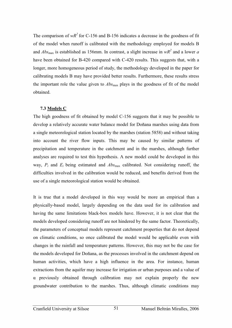
Cranfield University at Silsoe Manuel Beltrán Miralles, 2006 51
The comparison of wR2 for C-156 and B-156 indicates a decrease in the goodness of fit
of the model when runoff is calibrated with the methodology employed for models B
and Absmax is established as 156mm. In contrast, a slight increase in wR2 and a lower a
have been obtained for B-420 compared with C-420 results. This suggests that, with a
longer, more homogeneous period of study, the methodology developed in the paper for
calibrating models B may have provided better results. Furthermore, these results stress
the important role the value given to Absmax plays in the goodness of fit of the model
obtained.
7.3 Models C
The high goodness of fit obtained by model C-156 suggests that it may be possible to
develop a relatively accurate water balance model for Doñana marshes using data from
a single meteorological station located by the marshes (station 5858) and without taking
into account the river flow inputs. This may be caused by similar patterns of
precipitation and temperature in the catchment and in the marshes, although further
analyses are required to test this hypothesis. A new model could be developed in this
way, Pi and Ei being estimated and Absmax calibrated. Not considering runoff, the
difficulties involved in the calibration would be reduced, and benefits derived from the
use of a single meteorological station would be obtained.
It is true that a model developed in this way would be more an empirical than a
physically-based model, largely depending on the data used for its calibration and
having the same limitations black-box models have. However, it is not clear that the
models developed considering runoff are not hindered by the same factor. Theoretically,
the parameters of conceptual models represent catchment properties that do not depend
on climatic conditions, so once calibrated the model would be applicable even with
changes in the rainfall and temperature patterns. However, this may not be the case for
the models developed for Doñana, as the processes involved in the catchment depend on
human activities, which have a high influence in the area. For instance, human
extractions from the aquifer may increase for irrigation or urban purposes and a value of
α previously obtained through calibration may not explain properly the new
groundwater contribution to the marshes. Thus, although climatic conditions may

Cranfield University at Silsoe Manuel Beltrán Miralles, 2006 52
remain constant, the parameters calibrated may not be successfully employed in the
middle term due to changes in human activities, a factor that affects all the models
developed in this paper, not only models C.
7.4 Analysis of the residuals in relation to the phases of the marshes annual
hydrological cycle.
The goodness of fit of the models developed is higher in all cases for the final phases of
the cycle (phases 4 and 5), with a low wR2 returned for phases 1 and 3. The poor
performance of the models for phase 1 is caused by the difficulties involved in the
simulation of the flood extent when only small areas are flooded. Water inputs
(especially runoff) are not homogeneously distributed within the marshes and certain
areas flood before others; furthermore, some areas are artificially irrigated, all these
influences not being considered by the model. Regarding phase 3, the reasons for the
low wR2 are not clear, but may be related to human actions influencing discharges to the
Guadalquivir River or to the value given to the maximum possible flood extent.
7.5 Estimation of other variables
The visual analysis of the residuals plots (figures 6.5, 6.7, 6.9, 6.11 and 6.13) indicates
that the models developed, except for C-420, tend to overestimate the flood extent, a
trend confirmed by the analysis of the b and a coefficients of the regression: except for
model C-420, b is lower than 1 and a is negative. This general overestimation might be
caused by an underestimation of the evaporation values. Evaporation estimation
assigned a Kc value of 1.05 to the marshes, value for open water shallower than two
metres, although some areas of the marshes are covered with vegetation, which can
influence the evapotranspiration process. Data from evaporation pans exist for the area
from 2004 onwards. It should be determined whether these data could be used to
calibrate the Kc coefficient and obtain a more accurate estimation of the evaporation in
the marshes.
The calculation of tc employed the Kirpich equation, which is an empirical equation
calibrated for seven rural catchments in Tennessee (U.S.). Although this equation has

Cranfield University at Silsoe Manuel Beltrán Miralles, 2006 53
been employed in different catchments, it may not provide accurate results in the case of
Doñana, and other methods should be used in order to validate the results obtained.
Certain areas of the marshes are artificially flooded during some parts of the year,
increasing the errors of the model. Furthermore, the discharge from the marshes to the
Guadalquivir River is a difficult process to model. In addition, the model assumes that
the soils are completely dry at the beginning of the hydrologic year, although summer
storms may occur.
Smax and Imax were estimated as an average of their values before and after 25th April
1998. However, different values could have been used for the two periods and in this
way the goodness of fit of the model might have increased, a fact that stresses the
difficulties involved in the estimation of the Témez parameters.
Calibration and sensitivity analysis were manually conducted. Slight improvements in
the results obtained might be achieved by using tools such as Excel “Solver”.
Sensitivity analysis of model B-420 could have been expanded to Absmax, varying it
within its possible range 374-476 mm.
Finally, the calibration of model A was conducted following as criterion the
maximisation of R2, whereas calibration of models B-156 and B-420 was based on the
minimisation of the sum of squares of the residuals. Although both criteria are correct
and used in hydrology, it would have been a more consistent approach to use the
weighted R2 in both cases, since it is the efficiency criterion used for the assessment of
the models. In this way, it might have been possible to obtain a better estimation of
Absmax using the River Meca parameters.

Cranfield University at Silsoe Manuel Beltrán Miralles, 2006 54

Cranfield University at Silsoe Manuel Beltrán Miralles, 2006 55
8 CONCLUSIONS AND RECOMMENDATIONS
The analyses conducted show that it is possible to develop a model for simulating the
variation in the flood extent of Doñana marshes using for its calibration flood extent
data obtained from satellite images. The goodness of fit achieved is variable between
models, it largely depending on the variables calibrated and on the values given to the
other variables.
The calibration of either Absmax or rainfall-runoff model parameters involves difficulties
due to the need of estimating the other variables, a process that leads to inaccuracies in
the model obtained. On the one hand, the calibration of the rainfall-runoff model for
Doñana is difficult due to the lack of reliable and complete runoff data. The
methodology employed for its calibration offers the potential to calibrate runoff
parameters properly, but requires a longer period of study than used in this study.
Otherwise, some of the parameters must be estimated, a process that introduces errors in
the model. In addition, the results largely depend on the value estimated for Absmax. On
the other hand, the calibration of Absmax is a difficult process as it involves estimating
Témez parameters. In this case, the use of parameters calibrated for the Meca River has
not led to the calibration of a suitable Absmax value. Parameters calibrated for other
catchments may be applicable, but it might be difficult to find a useful catchment for
this purpose as these parameters are influenced not only by physical properties but also
by human activities in the catchment.
In addition, the analyses suggest that accurate results may be obtained through a model
that considers climate data from a single meteorological station located by the marshes
(station 5858) and does not take into account river flow inputs. It is recommended to
develop and calibrate a new model using this methodology and assess its performance
against the models developed in this study, assessing especially the way it simulates the
different phases of the marshes annual hydrological cycle. Special attention should be
played in future studies to the estimation of the evaporation, a difficult variable to
estimate that might have been underestimated in this study.

Cranfield University at Silsoe Manuel Beltrán Miralles, 2006 56

Cranfield University at Silsoe Manuel Beltrán Miralles, 2006 57
9 REFERENCES
Allen, R.G., Pereira, L.S., Raes, D. & Smith, M. (1998). Crop Evapotranspiration:
Guidelines for Computing Crop Water Requirements. FAO Irrigation and Drainage
Paper 56. Rome: FAO.
Aragonés D., Diaz-Delgado, R., Bustamante, J. (2005). Tratamiento de una serie
temporal larga de imágenes Landsat para la cartografia de inundación histórica de las
marismas de Doñana. Actas del XI Congreso Nacional de Teledetección. Tenerife, 21-
23 septiembre 2005.
Bayán, B.J. (2005) Los caminos del agua en la Marisma: los cambios en la red
hidrológica. In: García, F. & Martín, C. (Eds) (2005). Doñana: Agua y Biosfera.
Madrid: Confederación Hidrográfica del Guadalquivir, Ministerio de Medio Ambiente,
143-150
Beven, K.J., (2001) Rainfall-Runoff modeling: The primer. Chichester: Wiley.
Bustamante, J., Diaz-Delgado, R., Aragonés, D. & Pacios, F. (2006). Cambios en la
dinámica hídrica de la marisma de Doñana, In: Aguilera, E. Reconstrucción de las
fluctuaciones poblacionales de las aves de Doñana a lo largo de las últimas tres
decadas. Sevilla, Estación Biológica de Doñana, Consejo Superior de Investigaciones
Científicas.
Casas, J. & Urdiales, C. (1995). Introducción a la gestión hidraúlica de las marismas
del Parque Nacional de Doñana (SO de España). In: "Bases ecológicas para la
restauración de humedales en la cuenca mediterránea". Sevilla, Consejería de Medio
Ambiente, Junta de Andalucía, 165-189
Clemente, L., García, L.V. & Siljestrom, P. (1998). Los suelos del Parque Nacional de
Doñana. Madrid: Organismo Autónomo Parques Nacionales, Ministerio de Medio
Ambiente.

Cranfield University at Silsoe Manuel Beltrán Miralles, 2006 58
Delgado, M.D. (2005). Estimación del balance hídrico de la cuenca del río Caroní
mediante un modelo conceptual. Ph.D. thesis, Universidad Simón Bolivar. (Accessed: 9
June 2006)
http://www.cesma.usb.ve/reportes/2005-02.pdf
García, F. & Martín, C. (Eds) (2005). Doñana: Agua y Biosfera. Madrid: Confederación
Hidrográfica del Guadalquivir, Ministerio de Medio Ambiente.
García, J.I., Mintegui, J.A. & Robredo, J.C. (2005) La vegetación en la marisma del
Parque Nacional de Doñana en relación con sun régimen hidráulico. Madrid:
Organismo Autónomo Parques Nacionales, Ministerio de Medio Ambiente.
Gavilán, P., Lorite, I.J., Tornero, S. & Berenjena, J. (2005). Regional calibration of
Hargreaves equation for estimating referente ET in a semiarid environment.
Agricultural Water Management 81 (2006) 257-281
Gumbritch, T., Wolski, P., Frost, P. & McCarthy, T.S. (2004). Forecasting the spatial
extent of the annual flood in the Okavango delta, Botswana. Journal of Hydrology 290
(2004) 178–191
Hargreaves G.H. & Samani, Z.A. (1985). Reference crop evapotranspiration from
temperature. Applied Engineering in Agriculture 1(2), 96-97 As cited in Gavilán, P.,
Lorite, I.J., Tornero, S. & Berenjena, J. (2005). Regional calibration of Hargreaves
equation for estimating referente ET in a semiarid environment. Agricultural Water
Management 81 (2006) 257-281
Irmak S. & Haman, D.Z. (2003). Evapotranspiration: Potential or Reference? ABE 343
Agricultural and Biological Engineering Department, Florida Cooperative Extension
Service, Institute of Food and Agricultural Sciences, University of Florida. (Accessed:
15 June 2006)
http://edis.ifas.ufl.edu/pdffiles/AE/AE25600.pdf

Cranfield University at Silsoe Manuel Beltrán Miralles, 2006 59
Junta de Andalucía, (1999). Usos y coberturas vegetales del suelo. Sevilla: Consejería
de Medio Ambiente, Junta de Andalucía.
Junta de Andalucía, (2002). MDT 10x10 de Andalucía, vuelo 2001-2002.Sevilla:
Consejería de Agricultura y Pesca, Consejería de Medio Ambiente y Consejería de
Obras Públicas y Transporte, Junta de Andalucía.
Junta de Andalucía, (2004). Ortofotografía digital en color. Provincia de Huelva.
Sevilla: Consejería de Obras Públicas y Transporte, Junta de Andalucía.
Kirpich Z.P., (1940) Time of concentration of small agricultural watersheds, Civil
Engineering, 10(6):362. As cited in Verstraeten, G. & Poesen, J. (2001). Modelling the
long-term sediment trap efficiency of small ponds. Hydrological Processes 15 (2001)
2797-2819
Krause, P., Boyle, D.P. & Bäse, F. (2005). Comparison of different criteria for
hydrological model assessment. Advances in Geosciences 5 (2005) 89-97
Liu, W.T.H., Ayres, F.M., Santiami, E.L. & Kanazawa, P.J. (2003). Pantanal inundation
area prediction from space. Anais XI SBSR, Belo Horizonte, Brasil, 05 - 10 abril 2003,
INPE, 2523 - 2530.
MMA (Ministerio de Medio Ambiente), (2000). Libro Blanco del Agua en España.
Madrid: Ministerio de Medio Ambiente
Oliveira, R. (1998). Modelo hidrológico de precipitação-escoamento. (Accessed: 14
May 2006)
http://www.gesaq.org/documents/GESAQ_RH_Temez.pdf
Palmer, W. C., (1965). Meteorologic Drought. Res pap.45, U.S. Weather Bureau. As
cited in Verdú, J. (2004) Water balance modeling of the river Meca at Huelva, Spain.
MSc thesis, Cranfield University at Silsoe.

Cranfield University at Silsoe Manuel Beltrán Miralles, 2006 60
Ramsar (2002). Ramsar Site Information Sheet. (Accessed: 12 June 2006)
http://www.wetlands.org/RSDB/_COP9Directory/Directory/6cr006.html
Roshier, D.A., Whetton, P. H., Allan, R.J. & Robertson, A.I. (2001). Distribution and
persistence of temporary wetland habitats in arid Australia in relation to climate. Austral
Ecology 26, 371-384
Ruíz, J.M. (2000). Modelo distribuido para la evaluación de recursos hídricos. Madrid:
CEDEX. As cited in: Verdú, J. (2004) Water balance modeling of the river Meca at
Huelva, Spain. MSc thesis, Cranfield University at Silsoe.
Sahuquillo, A., Carrera, J., Samper, J., & Custodio, E. (1991) Revisión crítica de los
trabajos existentes de modelación del flujo subterráneo en el acuífero circundante al
Parque Nacional de Doñana. In: Curso Internacional de Hidrología Subterránea.
Barcelona: September 1991.
Schaap, M.G., Leij, F.J. & van Genuchten, M. T. (2001). Rosetta: a computer program
for estimating soil hydraulic parameters with hierarchical pedotransfer functions.
Journal of Hydroogy. 251:163-176.
Spanish Geological Survey, (?). Medio Físico del Parque Nacional de Doñana:
Hidrología e Hidrogeología. (Accessed: 8 April 2006)
http://aguas.igme.es/zonas_humedas/donana/medio_fisico/hidrologia.htm
Témez, J.R. (1977) Modelo Matemático de Transformación Precipitación-Aportación.
As cited in Verdú-Vazquez, J. (2004) Water balance modeling of the river Meca at
Huelva, Spain. MSc thesis, Cranfield University at Silsoe.
Verdú, J. (2004) Water balance modeling of the river Meca at Huelva, Spain. MSc
thesis, Cranfield University at Silsoe.

Cranfield University at Silsoe Manuel Beltrán Miralles, 2006 61
Xu, C. (2003) Hydrologic models. Department of Earth Sciences, Uppsala University.
(Accessed: 6 June 2006) http://folk.uio.no/chongyux/papers/CHAPTER-6.pdf
WWF/Adena (2006). Doñana y Cambio Climático: propuestas para la mitigación de
los efectos. (Accessed: 19 May 2006)
http://www.wwf.es/descarga/descarga_genetsis/INFORMECOMPLETO.pdf

Cranfield University at Silsoe Manuel Beltrán Miralles, 2006 62

Cranfield University at Silsoe Manuel Beltrán Miralles, 2006 63
APPENDIX A
TÉMEZ MODEL EQUATIONS
The following lines show the equations employed by the Témez model, as described by
Verdú (2004) and Oliveira (1998).
The surplus flow in the day i (Xi) is calculated as:
- 0=iX if oi PP ≤ (1)
-
oi
oii
PP
PPX
⋅−+
−=
2
)( 2
δ if oi PP > (2)
with δ calculated as:
- ii EPSS +−= −1maxδ
where Smax is the maximum moisture storage capacity of the soil in mm, Si-1 is the
available moisture in the soil during the day I-1 in mm and EPi is the potential
evapotranspiration in the catchment during the day i.
Therefore, runoff is only generated when rainfall is higher than Po,, which is calculated
as:
- )( 1max −−⋅= io SScP (3)
where c is a surplus parameter.
The actual evapotranspiration in the catchment (Ei, in mm) is limited by the potential
evapotranspiration (EPi) and by the water available in the unsaturated area
- ),(min 1 iiiii EPXPSE −+⋅= − (4)
The available moisture in the soils (Si, in mm) can be obtained as:
- ),0(max 1 iiiii EPXPSS −−+⋅= − (5)
The surplus flow generated is divided into surface runoff (Ai, in mm) and infiltration (Ii,
in mm), the latter depending on the maximum infiltration parameter (Imax, in mm)

Cranfield University at Silsoe Manuel Beltrán Miralles, 2006 64
-
max
maxIX
XII
i
i
i +⋅= (6)
- iii IXA −= (7)
Baseflow calculation is based on two hypotheses:
- The aquifer discharge is exponential
- Infiltration is concentrated during the midday.
Baseflow (Bi, in mm) is then calculated as:
- 2/
1
αε α −−− ⋅⋅+⋅= eIeBB iii (8)
At last, the total runoff generated (Ri, in mm) is calculated as:
- iii BAR += (9)
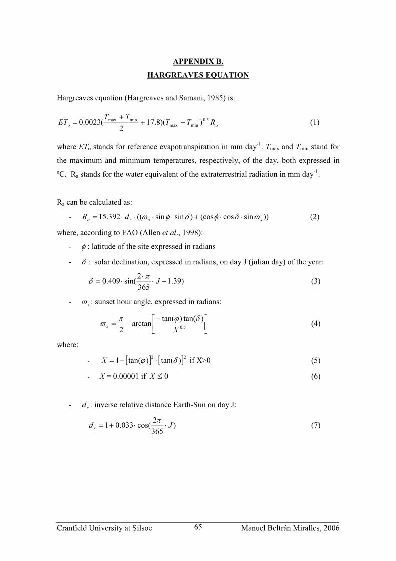
Cranfield University at Silsoe Manuel Beltrán Miralles, 2006 65
APPENDIX B.
HARGREAVES EQUATION
Hargreaves equation (Hargreaves and Samani, 1985) is:
ao RTTTT
ET 5.0
minmax
minmax ))(8.172
(0023.0 −++
= (1)
where ETo stands for reference evapotranspiration in mm day-1. Tmax and Tmin stand for
the maximum and minimum temperatures, respectively, of the day, both expressed in
ºC. Ra stands for the water equivalent of the extraterrestrial radiation in mm day-1.
Ra can be calculated as:
- ))sincos(cos)sinsin((392.15 ssra dR ωδφδφω ⋅⋅+⋅⋅⋅⋅= (2)
where, according to FAO (Allen et al., 1998):
- φ : latitude of the site expressed in radians
- δ : solar declination, expressed in radians, on day J (julian day) of the year:
)39.1365
2sin(409.0 −⋅
⋅⋅= J
πδ (3)
- sω : sunset hour angle, expressed in radians:
−−=5.0
)tan()tan(arctan
2 Xs
δϕπϖ (4)
where:
- [ ] [ ]22)tan()tan(1 δϕ ⋅−=X if X>0 (5)
- X = 0.00001 if 0≤X (6)
- rd : inverse relative distance Earth-Sun on day J:
)365
2cos(033.01 Jd r ⋅⋅+=
π (7)

Cranfield University at Silsoe Manuel Beltrán Miralles, 2006 66
APPENDIX C
RELIEF OF THE CATCHMENT OF DOÑANA MARSHES
Derived from the “MDT 10x10 de Andalucía, vuelo 2001-2002” (Junta de Andalucía,
2002).

Cranfield University at Silsoe Manuel Beltrán Miralles, 2006 67
APPENDIX D
LITHOLOGY MAP OF THE CATCHMENT OF DOÑANA MARSHES
Derived from the MAGNA series of geologic maps for the area of the Spanish
Geological Survey.

Cranfield University at Silsoe Manuel Beltrán Miralles, 2006 68
APPENDIX E
LAND USE/LAND COVER MAP OF THE CATCHMENT OF DOÑANA
MARSHES
Derived from the “Usos y coberturas vegetales del suelo” map (Junta de Andalucía,
1999)

Cranfield University at Silsoe Manuel Beltrán Miralles, 2006 69
APPENDIX F.
PROCEDURE FOLLOWED FOR THE INFILLING OF THE
METEOROLOGICAL DATA GAPS
Data from thirteen pluviometric and eight thermometric stations were acquired in a first
step (tables F.1 and F.2), following as main criteria their location and data
completeness.
F.1 Pluviometric stations
Table F.1 - Characteristics of all pluviometric stations from which data was acquired.
Code Name Initial Year
Final Year
Altitude (m)
Longer Complete Sequence
2nd Longer Complete Sequence
4 622* La Palma Condado 1955 2004 92 1967-2004 1956-1965
4 628* Lucena Del Puerto 1964 2004 80 1967-1984 1986-1999
5 822* Castillo Guardas 1985 2004 351 1997-2004 1993-1995
5 824
Gerena ‘Aforos
Guadiamar’ 1986 2004 130 1996-2004 1993-1993
5 826*
Escacena Campo
‘Las Contiendas’ 1948 2004 417 1953-1961 1997-2004
5 831
Escacena Campo
‘Hytasa’ 1954 2004 130 1997-2002 1991-1994
5 833O
Aznalcazar ‘La
Juncosa’ 1976 2004 20 1977-1997 1999-2004
5 842 Hinojos ‘La Calera’ 1986 2004 41 1997-1999 2002-2004
5 843*
Villamanrique
Cond.'Juncosilla 1949 2004 20 1986-1989 1996-1999
5 858* Almonte ‘Doñana’ 1967 2004 5 1993-1997 1982-1985
5 859C
Aznalcazar ‘Casilla
Brenes’ 1985 2004 4 1992-1995 1997-2000
5 859E
Almonte
‘Marismillas’ 1984 2001 10 1995-1998 1992-1993
5 860G
Almonte
‘Acebuche’ 1984 2004 47 1992-1995 1997-1999
* Stations finally employed in the model.
Precipitation data gaps of the six pluviometric stations finally selected were infilled
trough the following process. Firstly, the average precipitation for each day was
calculated using the thirteen pluviometric stations. For each of the six selected stations
was then calculated the R2 of the correlation between:
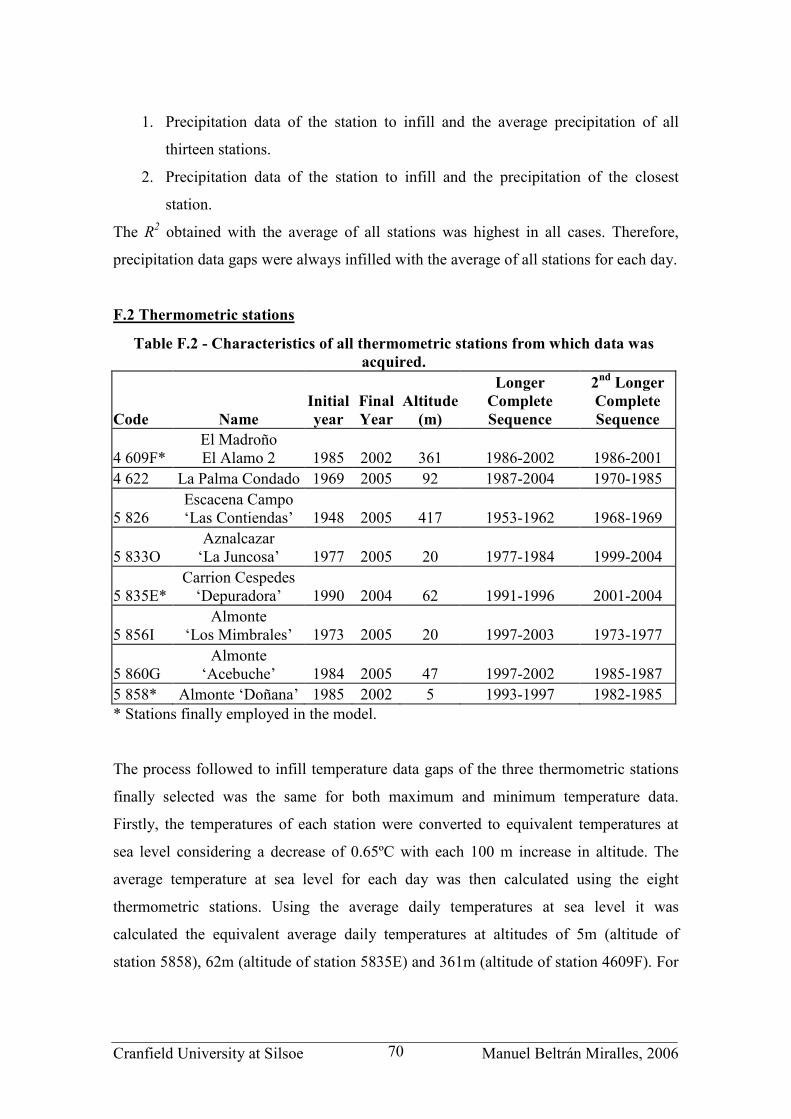
Cranfield University at Silsoe Manuel Beltrán Miralles, 2006 70
1. Precipitation data of the station to infill and the average precipitation of all
thirteen stations.
2. Precipitation data of the station to infill and the precipitation of the closest
station.
The R2 obtained with the average of all stations was highest in all cases. Therefore,
precipitation data gaps were always infilled with the average of all stations for each day.
F.2 Thermometric stations
Table F.2 - Characteristics of all thermometric stations from which data was acquired.
Code Name Initial year
Final Year
Altitude (m)
Longer Complete Sequence
2nd Longer Complete Sequence
4 609F*
El Madroño
El Alamo 2 1985 2002 361 1986-2002 1986-2001
4 622 La Palma Condado 1969 2005 92 1987-2004 1970-1985
5 826
Escacena Campo
‘Las Contiendas’ 1948 2005 417 1953-1962 1968-1969
5 833O
Aznalcazar
‘La Juncosa’ 1977 2005 20 1977-1984 1999-2004
5 835E*
Carrion Cespedes
‘Depuradora’ 1990 2004 62 1991-1996 2001-2004
5 856I
Almonte
‘Los Mimbrales’ 1973 2005 20 1997-2003 1973-1977
5 860G
Almonte
‘Acebuche’ 1984 2005 47 1997-2002 1985-1987
5 858* Almonte ‘Doñana’ 1985 2002 5 1993-1997 1982-1985
* Stations finally employed in the model.
The process followed to infill temperature data gaps of the three thermometric stations
finally selected was the same for both maximum and minimum temperature data.
Firstly, the temperatures of each station were converted to equivalent temperatures at
sea level considering a decrease of 0.65ºC with each 100 m increase in altitude. The
average temperature at sea level for each day was then calculated using the eight
thermometric stations. Using the average daily temperatures at sea level it was
calculated the equivalent average daily temperatures at altitudes of 5m (altitude of
station 5858), 62m (altitude of station 5835E) and 361m (altitude of station 4609F). For

Cranfield University at Silsoe Manuel Beltrán Miralles, 2006 71
each of the three stations it was calculated the R2 of the correlations between
temperature data of:
1. Each station and the closest thermometric stations, the latter being corrected to
the equivalent altitude.
2. Each station and the equivalent average temperature at the station altitude.
Station 4609F gaps were infilled using the average of all thermometric stations in the
catchment for each. Station 5835E was infilled using the equivalent at 62m altitude of
the daily data from station 5833O. The data gaps still existing after this process were
infilled using the average of all thermometric stations in the catchment for the day.
Station 5858 was infilled using the equivalent at 5m altitude of the average of the
temperatures of the stations 5856I and 5860 G for the day.
Figure F.1 Location of the thirteen
pluviometric stations.
Figure F.2 Location of the eight
thermometric stations.
Figure F.3 represent the degree of completeness of the different stations for which data
was available. Gaps in the color line represent data gaps of at least one month.

Cranfield University at Silsoe Manuel Beltrán Miralles, 2006 72
Year 1994 1995 1996
Month J F M A M J J A S O N D J F M A M J J A S O N D J F M A M J J A S O N D
Station
4622
4628
5822
5824
5826
5831
5833O
5842
5843
5858
5859C
5859E
5860G
Year 1997 1998 1999
Month J F M A M J J A S O N D J F M A M J J A S O N D J F M A M J J A S O N D
Station
4622
4628
5822
5824
5826
5831
5833O
5842
5843
5858
5859C
5859E
5860G
Figure F.3- Degree of data completeness of the meteorological stations during the
period 1994-1999. Periods in white represent data gaps in the acquired data of at
least one month.

Cranfield University at Silsoe Manuel Beltrán Miralles, 2006 73
Year 2000 2001 2002
Month J F M A M J J A S O N D J F M A M J J A S O N D J F M A M J J A S O N D
Station
4622
4628
5822
5824
5826
5831
5833O
5842
5843
5858
5859C
5859E
5860G
Year 2003 2004
Month J F M A M J J A S O N D J F M A M J J A S O N D
Station
4622
4628
5822
5824
5826
5831
5833O
5842
5843
5858
5859C
5859E
5860G
Figure F.4- Degree of data completeness of the meteorological stations during the
period 2000-2004. Periods in white represent data gaps in the acquired data of at
least one month.

Cranfield University at Silsoe Manuel Beltrán Miralles, 2006 74
APPENDIX G
WATERCOURSES EMPLOYED FOR THE CALCULATION OF THE TIME
OF CONCENTRATION
Derived from the “Ortofotografía Digital en Color. Provincia de Huelva” (Junta de
Andalucía, 2004).

Cranfield University at Silsoe Manuel Beltrán Miralles, 2006 75
APPENDIX H.
DATA EMPLOYED AND CALCULATIONS CONDUCTED FOR THE
ESTIMATION OF SMAX FROM PUBLISHED SOIL ANALYSES
Data necessary for the Smax calculation was obtained from soil analysis published by
Clemente et al. (1998). From these analyses it was obtained the % sands, % silt and %
clay for seven soils included within the Doñana marshes from the most common soils
classifications: Salorthids and Aeric Fluvaquents. It was also obtained the depth of the
water table at the end of the dry season. Smax was calculated for each horizon located
above the water table at the end of the dry season using equation (1):
)()()(max mmdepthmmS rs ⋅−= θθ (1)
θr and θs were obtained through a pedotransfer function that uses soil texture data as
predictor (Schaap et al., 2001). The pedotransfer function was run through the Rosetta
software, free software developed by the United States Salinity Laboratory that can be
downloaded from http://www.ars.usda.gov/Services/docs.htm?docid=8953.
The numeration employed by Clemente et al. (1998) for designating the different
profiles and horizons has been kept.
Table H.1- Soil properties used for Smax calculation (1/2). Profile
Horizon
Sands (%)
Silt (%)
Clay (%)
θθθθr (cm3/cm3
θθθθs (cm3/cm3)
Depth (m)
Smax (mm)
Soil Class
38 1.40 566 S
38.1 0.4 68.5 31.1 0.0912 0.4827 0.15 59
38.2 0.3 34.2 65.6 0.1079 0.5274 0.15 63
38.3 0.1 52.6 47.3 0.1060 0.5175 0.15 62
38.4 0.2 47.2 52.6 0.1075 0.5214 0.20 83
38.5 0.1 68.1 31.8 0.0921 0.4848 0.30 118
38.6 0.2 51.9 48.0 0.1063 0.5183 0.30 124
38.7 0.3 71.2 28.6 0.0887 0.4779 0.15 58
39 1.10 409 S
39.1 0.9 45.9 53.1 0.1071 0.5199 0.10 41
39.2 0.3 49 50.6 0.1070 0.5195 0.20 83
39.3 0.9 46 53.1 0.1071 0.5203 0.10 41
39.4 0.4 56.4 43.1 0.1034 0.5111 0.15 61
39.5 1.3 53.1 45.6 0.1045 0.5133 0.25 102
39.6 0.3 61.6 38.1 0.0986 0.5007 0.20 80 S: Salorthids AF: Aeric Fluvaquents

Cranfield University at Silsoe Manuel Beltrán Miralles, 2006 76
Table H.2- Soil properties used for Smax calculation (2/2). Profile
Horizon
Sands (%)
Silt (%)
Clay (%)
θθθθr (cm3/cm3
θθθθs (cm3/cm3)
Depth (m)
Smax (mm)
Soil Class
40 1.00 454 S
40.1 0.7 36.2 63.1 0.1076 0.5257 0.15 63
40.2 1.4 53 45.6 0.1045 0.5131 0.20 82
40.3 0.4 49 50.6 0.1070 0.5196 0.65 268
40.4 0.8 53.6 45.6 0.1048 0.5143 0.10 41
41 1.00 446 S
41.1 3.8 43.1 53.1 0.1052 0.5143 0.03 12
41.2 3.5 60.9 35.6 0.0948 0.4898 0.10 39
41.3 0.3 44.1 55.6 0.1078 0.5230 0.27 112
41.4 0.2 54.2 45.6 0.1051 0.5154 0.25 103
41.5 0.6 56.3 43.1 0.1033 0.5111 0.15 61
41.6 0.4 66.5 33.1 0.0933 0.4876 0.30 118
45 0.90 373 AF
45.1 2.6 34.2 63.3 0.1063 0.5223 0.05 21
45.2 1.1 30.9 68.0 0.1072 0.5258 0.15 63
45.3 2.0 40.3 57.8 0.1068 0.5212 0.15 62
45.4 2.0 41.4 56.6 0.1067 0.5202 0.15 62
45.4 1.3 43.4 55.4 0.1072 0.5212 0.30 124
45.5 1.6 44.2 54.2 0.1068 0.5195 0.10 41
46 1.00 416 AF
46.1 1.1 60.1 38.8 0.0991 0.5013 0.05 20
46.2 1.7 26.3 72.1 0.1067 0.5247 0.15 63
46.3 1.0 35.7 63.3 0.1074 0.5252 0.30 125
46.4 1.0 41.0 58.0 0.1074 0.5230 0.30 125
46.5 0.2 44.0 55.8 0.1079 0.5233 0.20 83
47 0.50 266 S
47.1 4.6 57.3 38.1 0.0972 0.4945 0.10 40
47.2 1.3 50.6 48.1 0.1056 0.5158 0.35 144
47.3 0.3 46.6 53.1 0.1060 0.5175 0.20 82
S: Salorthids AF: Aeric Fluvaquents
Smax for most soils varies between 373 mm and 446 mm. Values of 566 mm and 266
mm corresponded to soils were the water table at the end of the dry season was,
respectively, particularly low (1.4m) or high (0.50m). These water table levels were
infrequent in the analyses reviewed, so were excluded from the Smax calculation, which
was conducted as the average of the values obtained for the others soil profiles:
mmS 4205
416373446454409max =
++++=
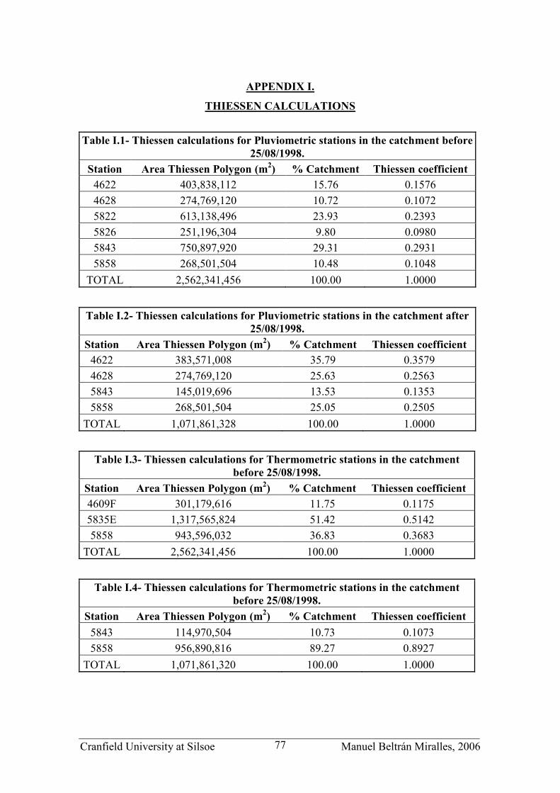
Cranfield University at Silsoe Manuel Beltrán Miralles, 2006 77
APPENDIX I.
THIESSEN CALCULATIONS
Table I.1- Thiessen calculations for Pluviometric stations in the catchment before 25/08/1998.
Station Area Thiessen Polygon (m2) % Catchment Thiessen coefficient
4622 403,838,112 15.76 0.1576
4628 274,769,120 10.72 0.1072
5822 613,138,496 23.93 0.2393
5826 251,196,304 9.80 0.0980
5843 750,897,920 29.31 0.2931
5858 268,501,504 10.48 0.1048
TOTAL 2,562,341,456 100.00 1.0000
Table I.2- Thiessen calculations for Pluviometric stations in the catchment after 25/08/1998.
Station Area Thiessen Polygon (m2) % Catchment Thiessen coefficient
4622 383,571,008 35.79 0.3579
4628 274,769,120 25.63 0.2563
5843 145,019,696 13.53 0.1353
5858 268,501,504 25.05 0.2505
TOTAL 1,071,861,328 100.00 1.0000
Table I.3- Thiessen calculations for Thermometric stations in the catchment before 25/08/1998.
Station Area Thiessen Polygon (m2) % Catchment Thiessen coefficient
4609F 301,179,616 11.75 0.1175
5835E 1,317,565,824 51.42 0.5142
5858 943,596,032 36.83 0.3683
TOTAL 2,562,341,456 100.00 1.0000
Table I.4- Thiessen calculations for Thermometric stations in the catchment before 25/08/1998.
Station Area Thiessen Polygon (m2) % Catchment Thiessen coefficient
5843 114,970,504 10.73 0.1073
5858 956,890,816 89.27 0.8927
TOTAL 1,071,861,320 100.00 1.0000

Cranfield University at Silsoe Manuel Beltrán Miralles, 2006 78
APPENDIX J
SIMULATION OF THE DAILY FLOOD EXTENT FOR THE DIFFERENT
MODELS DEVELOPED.
Model A
1996-1997
0.0E+00
5.0E+07
1.0E+08
1.5E+08
2.0E+08
2.5E+08
3.0E+08
3.5E+08
01/09/1996
21/09/1996
11/10/1996
31/10/1996
20/11/1996
10/12/1996
30/12/1996
19/01/1997
08/02/1997
28/02/1997
20/03/1997
09/04/1997
29/04/1997
19/05/1997
08/06/1997
28/06/1997
18/07/1997
07/08/1997
27/08/1997
Date
Flood
exten
t (m2 )
Simulated
Observed
Figure J.1- Flood extent simulated by model A for the hydrologic year 1996-1997.
1998-1999
0.0E+00
5.0E+07
1.0E+08
1.5E+08
2.0E+08
2.5E+08
3.0E+08
3.5E+08
01/09/1998
21/09/1998
11/10/1998
31/10/1998
20/11/1998
10/12/1998
30/12/1998
19/01/1999
08/02/1999
28/02/1999
20/03/1999
09/04/1999
29/04/1999
19/05/1999
08/06/1999
28/06/1999
18/07/1999
07/08/1999
27/08/1999
Date
Flood
extent (m
2 )
Simulated
Observed
Figure J.2- Flood extent simulated by model A for the hydrologic year 1998-1999.

Cranfield University at Silsoe Manuel Beltrán Miralles, 2006 79
2000-2001
0.0E+00
5.0E+07
1.0E+08
1.5E+08
2.0E+08
2.5E+08
3.0E+08
3.5E+08
01/09/2000
21/09/2000
11/10/2000
31/10/2000
20/11/2000
10/12/2000
30/12/2000
19/01/2001
08/02/2001
28/02/2001
20/03/2001
09/04/2001
29/04/2001
19/05/2001
08/06/2001
28/06/2001
18/07/2001
07/08/2001
27/08/2001
Date
Flood extent (m2 )
Simulated
Observed
Figure J.3- Model A flood extent simulation for the hydrologic year 2000-2001.
2002-2003
0.0E+00
5.0E+07
1.0E+08
1.5E+08
2.0E+08
2.5E+08
3.0E+08
3.5E+08
01/09/2002
21/09/2002
11/10/2002
31/10/2002
20/11/2002
10/12/2002
30/12/2002
19/01/2003
08/02/2003
28/02/2003
20/03/2003
09/04/2003
29/04/2003
19/05/2003
08/06/2003
28/06/2003
18/07/2003
07/08/2003
27/08/2003
Date
Flood
exten
t (m2 )
Simulated
Observed
Figure J.4- Model A flood extent simulation for the hydrologic year 2002-2003.
2003-2004
0.0E+00
5.0E+07
1.0E+08
1.5E+08
2.0E+08
2.5E+08
3.0E+08
3.5E+08
01/09/2003
21/09/2003
11/10/2003
31/10/2003
20/11/2003
10/12/2003
30/12/2003
19/01/2004
08/02/2004
28/02/2004
19/03/2004
08/04/2004
28/04/2004
18/05/2004
07/06/2004
27/06/2004
17/07/2004
06/08/2004
26/08/2004
Date
Flood
extent (m2 )
Simulated
Observed
Figure J.5- Model A flood extent simulation for the hydrologic year 2003-2004.

Cranfield University at Silsoe Manuel Beltrán Miralles, 2006 80
Model B-156
1996-1997
0.0E+00
5.0E+07
1.0E+08
1.5E+08
2.0E+08
2.5E+08
3.0E+08
3.5E+08
01/09/1996
21/09/1996
11/10/1996
31/10/1996
20/11/1996
10/12/1996
30/12/1996
19/01/1997
08/02/1997
28/02/1997
20/03/1997
09/04/1997
29/04/1997
19/05/1997
08/06/1997
28/06/1997
18/07/1997
07/08/1997
27/08/1997
Date
Flood
extent (m2 )
Simulated
Observed
Figure J.6- Model B-156 flood extent simulation for the hydrologic year 1996-1997.
1998-1999
0.0E+00
5.0E+07
1.0E+08
1.5E+08
2.0E+08
2.5E+08
3.0E+08
3.5E+08
01/09/1998
21/09/1998
11/10/1998
31/10/1998
20/11/1998
10/12/1998
30/12/1998
19/01/1999
08/02/1999
28/02/1999
20/03/1999
09/04/1999
29/04/1999
19/05/1999
08/06/1999
28/06/1999
18/07/1999
07/08/1999
27/08/1999
Date
Flood
exten
t (m
2 )
Simulated
Observed
Figure J.7- Model B-156 flood extent simulation for the hydrologic year 1998-1999.
2000-2001
0.0E+00
5.0E+07
1.0E+08
1.5E+08
2.0E+08
2.5E+08
3.0E+08
3.5E+08
01/09/2000
21/09/2000
11/10/2000
31/10/2000
20/11/2000
10/12/2000
30/12/2000
19/01/2001
08/02/2001
28/02/2001
20/03/2001
09/04/2001
29/04/2001
19/05/2001
08/06/2001
28/06/2001
18/07/2001
07/08/2001
27/08/2001
Date
Flood
exten
t (m
2 )
Simulated
Observed
Figure J.8- Model B-156 flood extent simulation for the hydrologic year 2000-2001.

Cranfield University at Silsoe Manuel Beltrán Miralles, 2006 81
2002-2003
0.0E+00
5.0E+07
1.0E+08
1.5E+08
2.0E+08
2.5E+08
3.0E+08
3.5E+08
01/09/2002
21/09/2002
11/10/2002
31/10/2002
20/11/2002
10/12/2002
30/12/2002
19/01/2003
08/02/2003
28/02/2003
20/03/2003
09/04/2003
29/04/2003
19/05/2003
08/06/2003
28/06/2003
18/07/2003
07/08/2003
27/08/2003
Date
Flood
extent (m2 )
Simulated
Observed
Figure J.9- Model B-156 flood extent simulation for the hydrologic year 2002-2003.
2003-2004
0.0E+00
5.0E+07
1.0E+08
1.5E+08
2.0E+08
2.5E+08
3.0E+08
3.5E+08
01/09/2003
21/09/2003
11/10/2003
31/10/2003
20/11/2003
10/12/2003
30/12/2003
19/01/2004
08/02/2004
28/02/2004
19/03/2004
08/04/2004
28/04/2004
18/05/2004
07/06/2004
27/06/2004
17/07/2004
06/08/2004
26/08/2004
Date
Flood
extent (m2 )
Simulated
Observed
Figure J.10- Model B-156 flood extent simulation for the hydrologic year
2003-2004.
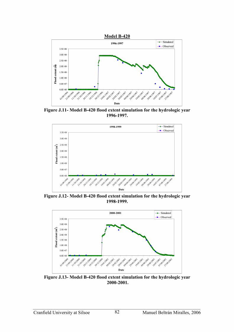
Cranfield University at Silsoe Manuel Beltrán Miralles, 2006 82
Model B-420
1996-1997
0.0E+00
5.0E+07
1.0E+08
1.5E+08
2.0E+08
2.5E+08
3.0E+08
3.5E+08
01/09/1996
21/09/1996
11/10/1996
31/10/1996
20/11/1996
10/12/1996
30/12/1996
19/01/1997
08/02/1997
28/02/1997
20/03/1997
09/04/1997
29/04/1997
19/05/1997
08/06/1997
28/06/1997
18/07/1997
07/08/1997
27/08/1997
Date
Flood extent (m2)
Simulated
Observed
Figure J.11- Model B-420 flood extent simulation for the hydrologic year
1996-1997.
1998-1999
0.0E+00
5.0E+07
1.0E+08
1.5E+08
2.0E+08
2.5E+08
3.0E+08
3.5E+08
01/09/1998
21/09/1998
11/10/1998
31/10/1998
20/11/1998
10/12/1998
30/12/1998
19/01/1999
08/02/1999
28/02/1999
20/03/1999
09/04/1999
29/04/1999
19/05/1999
08/06/1999
28/06/1999
18/07/1999
07/08/1999
27/08/1999
Date
Flood
exten
t (m
2)
Simulated
Observed
Figure J.12- Model B-420 flood extent simulation for the hydrologic year
1998-1999.
2000-2001
0.0E+00
5.0E+07
1.0E+08
1.5E+08
2.0E+08
2.5E+08
3.0E+08
3.5E+08
01/09/2000
21/09/2000
11/10/2000
31/10/2000
20/11/2000
10/12/2000
30/12/2000
19/01/2001
08/02/2001
28/02/2001
20/03/2001
09/04/2001
29/04/2001
19/05/2001
08/06/2001
28/06/2001
18/07/2001
07/08/2001
27/08/2001
Date
Flood
exten
t (m
2 )
Simulated
Observed
Figure J.13- Model B-420 flood extent simulation for the hydrologic year
2000-2001.

Cranfield University at Silsoe Manuel Beltrán Miralles, 2006 83
2002-2003
0.0E+00
5.0E+07
1.0E+08
1.5E+08
2.0E+08
2.5E+08
3.0E+08
3.5E+08
01/09/2002
21/09/2002
11/10/2002
31/10/2002
20/11/2002
10/12/2002
30/12/2002
19/01/2003
08/02/2003
28/02/2003
20/03/2003
09/04/2003
29/04/2003
19/05/2003
08/06/2003
28/06/2003
18/07/2003
07/08/2003
27/08/2003
Date
Flood
extent (m2 )
Simulated
Observed
Figure J.14- Model B-420 flood extent simulation for the hydrologic year
2002-2003.
2003-2004
0.0E+00
5.0E+07
1.0E+08
1.5E+08
2.0E+08
2.5E+08
3.0E+08
3.5E+08
01/09/2003
21/09/2003
11/10/2003
31/10/2003
20/11/2003
10/12/2003
30/12/2003
19/01/2004
08/02/2004
28/02/2004
19/03/2004
08/04/2004
28/04/2004
18/05/2004
07/06/2004
27/06/2004
17/07/2004
06/08/2004
26/08/2004
Date
Flood
extent (m2 )
Simulated
Observed
Figure J.15- Model B-420 flood extent simulation for the hydrologic year
2003-2004.

Cranfield University at Silsoe Manuel Beltrán Miralles, 2006 84
Model C-156
1996-1997
0.0E+00
5.0E+07
1.0E+08
1.5E+08
2.0E+08
2.5E+08
3.0E+08
3.5E+08
01/09/1996
21/09/1996
11/10/1996
31/10/1996
20/11/1996
10/12/1996
30/12/1996
19/01/1997
08/02/1997
28/02/1997
20/03/1997
09/04/1997
29/04/1997
19/05/1997
08/06/1997
28/06/1997
18/07/1997
07/08/1997
27/08/1997
Date
Flood
extent (m2)
Simulated
Observed
Figure J.16- Model C-156 flood extent simulation for the hydrologic year
1996-1997.
1998-1999
0.0E+00
5.0E+07
1.0E+08
1.5E+08
2.0E+08
2.5E+08
3.0E+08
3.5E+08
01/09/1998
21/09/1998
11/10/1998
31/10/1998
20/11/1998
10/12/1998
30/12/1998
19/01/1999
08/02/1999
28/02/1999
20/03/1999
09/04/1999
29/04/1999
19/05/1999
08/06/1999
28/06/1999
18/07/1999
07/08/1999
27/08/1999
Date
Flood
exten
t (m
2 )
Simulated
Observed
Figure J.17- Model C-156 flood extent simulation for the hydrologic year
1998-1999.
2000-2001
0.0E+00
5.0E+07
1.0E+08
1.5E+08
2.0E+08
2.5E+08
3.0E+08
3.5E+08
01/09/2000
21/09/2000
11/10/2000
31/10/2000
20/11/2000
10/12/2000
30/12/2000
19/01/2001
08/02/2001
28/02/2001
20/03/2001
09/04/2001
29/04/2001
19/05/2001
08/06/2001
28/06/2001
18/07/2001
07/08/2001
27/08/2001
Date
Flood
exten
t (m
2 )
Simulated
Observed
Figure J.18- Model C-156 flood extent simulation for the hydrologic year
2000-2001.

Cranfield University at Silsoe Manuel Beltrán Miralles, 2006 85
2002-2003
0.0E+00
5.0E+07
1.0E+08
1.5E+08
2.0E+08
2.5E+08
3.0E+08
3.5E+08
01/09/2002
21/09/2002
11/10/2002
31/10/2002
20/11/2002
10/12/2002
30/12/2002
19/01/2003
08/02/2003
28/02/2003
20/03/2003
09/04/2003
29/04/2003
19/05/2003
08/06/2003
28/06/2003
18/07/2003
07/08/2003
27/08/2003
Date
Flood
exten
t (m
2 )
Simulated
Observed
Figure J.19- Model C-156 flood extent simulation for the hydrologic year
2002-2003.
2003-2004
0.0E+00
5.0E+07
1.0E+08
1.5E+08
2.0E+08
2.5E+08
3.0E+08
3.5E+08
01/09/2003
21/09/2003
11/10/2003
31/10/2003
20/11/2003
10/12/2003
30/12/2003
19/01/2004
08/02/2004
28/02/2004
19/03/2004
08/04/2004
28/04/2004
18/05/2004
07/06/2004
27/06/2004
17/07/2004
06/08/2004
26/08/2004
Date
Flood
extent (m2 )
Simulated
Observed
Figure J.20- Model C-156 flood extent simulation for the hydrologic year
2003-2004.

Cranfield University at Silsoe Manuel Beltrán Miralles, 2006 86
Model C-420
1996-1997
0.0E+00
5.0E+07
1.0E+08
1.5E+08
2.0E+08
2.5E+08
3.0E+08
3.5E+08
01/09/1996
21/09/1996
11/10/1996
31/10/1996
20/11/1996
10/12/1996
30/12/1996
19/01/1997
08/02/1997
28/02/1997
20/03/1997
09/04/1997
29/04/1997
19/05/1997
08/06/1997
28/06/1997
18/07/1997
07/08/1997
27/08/1997
Date
Flood
extent (m2 )
Simulated
Observed
Figure J.21- Model C-420 flood extent simulation for the hydrologic year
1996-1997.
1998-1999
0.0E+00
5.0E+07
1.0E+08
1.5E+08
2.0E+08
2.5E+08
3.0E+08
3.5E+08
01/09/1998
21/09/1998
11/10/1998
31/10/1998
20/11/1998
10/12/1998
30/12/1998
19/01/1999
08/02/1999
28/02/1999
20/03/1999
09/04/1999
29/04/1999
19/05/1999
08/06/1999
28/06/1999
18/07/1999
07/08/1999
27/08/1999
Date
Flood
exten
t (m
2 )
Simulated
Observed
Figure J.22- Model C-420 flood extent simulation for the hydrologic year
1998-1999.
2000-2001
0.0E+00
5.0E+07
1.0E+08
1.5E+08
2.0E+08
2.5E+08
3.0E+08
3.5E+08
01/09/2000
21/09/2000
11/10/2000
31/10/2000
20/11/2000
10/12/2000
30/12/2000
19/01/2001
08/02/2001
28/02/2001
20/03/2001
09/04/2001
29/04/2001
19/05/2001
08/06/2001
28/06/2001
18/07/2001
07/08/2001
27/08/2001
Date
Flood
exten
t (m
2 )
Simulated
Observed
Figure J.23- Model C-420 flood extent simulation for the hydrologic year
2000-2001.

Cranfield University at Silsoe Manuel Beltrán Miralles, 2006 87
2002-2003
0.0E+00
5.0E+07
1.0E+08
1.5E+08
2.0E+08
2.5E+08
3.0E+08
3.5E+08
01/09/2002
21/09/2002
11/10/2002
31/10/2002
20/11/2002
10/12/2002
30/12/2002
19/01/2003
08/02/2003
28/02/2003
20/03/2003
09/04/2003
29/04/2003
19/05/2003
08/06/2003
28/06/2003
18/07/2003
07/08/2003
27/08/2003
Date
Flood
exten
t (m
2 )
Simulated
Observed
Figure J.24- Model C-420 flood extent simulation for the hydrologic year
2002-2003.
2003-2004
0.0E+00
5.0E+07
1.0E+08
1.5E+08
2.0E+08
2.5E+08
3.0E+08
3.5E+08
01/09/2003
21/09/2003
11/10/2003
31/10/2003
20/11/2003
10/12/2003
30/12/2003
19/01/2004
08/02/2004
28/02/2004
19/03/2004
08/04/2004
28/04/2004
18/05/2004
07/06/2004
27/06/2004
17/07/2004
06/08/2004
26/08/2004
Date
Flood
exten
t (m
2 )
Simulated
Observed
Figure J.25- Model C-420 flood extent simulation for the hydrologic year
2003-2004.

Cranfield University at Silsoe Manuel Beltrán Miralles, 2006 88
APPENDIX K
CD CONTENTS DESCRIPTION
Title of the files and description of the material contained in each folder included in the
cd:
Folder “Calibration”:
- Model A calibration.xls: Spreadsheet employed for the calibration of model A
- Model B-156 calibration.xls: Spreadsheet employed for the calibration of model
B-156
- Model B-420 calibration.xls: Spreadsheet employed for the calibration of model
B-420
Folder “Validation”:
- Model A Validation.xls: Spreadsheet employed for the calibration of model A
- Model B-156 Validation.xls: Spreadsheet employed for the calibration of model
B-156
- Model B-420 Validation.xls: Spreadsheet employed for the calibration of model
B-420
- Model C-156 Validation.xls: Spreadsheet employed for the calibration of model
C-156
- Model C-420 Validation.xls: Spreadsheet employed for the calibration of model
C-420
Folder “Volume”
- Volume.xls: Spreadsheet containing the volumes of water
Folder “Thesis”
- Mbeltran_thesis.pdf: Thesis in pdf format