course notes on computational financeseydel/cfcoursenotes2beam.pdf · seydel: course notes on...

Seydel: Course Notes on Computational Finan e, Chapter 2 (Version 2015) 200

Course Notes on

Computational Finance

2Random Numbers


2. Computation of Random Numbers

Definition (sample from a distribution)

A sequence of numbers is called sample from a distribution function F , if thenumbers are independent realizations of a random variable with distribution F .

Examples

If F is the uniform distribution on the interval [0, 1], then we call the samples fromF uniform deviates. Notation: ∼ U [0, 1].

If F is the standard normal distribution, then we call the samples from F standard

normal deviates. Notation: ∼ N (0, 1).

The basis of random number generation is to draw numbers ∼ U [0, 1].


2.1 Uniform Deviates

A. Linear Congruential Generators

Choose a, b,M ∈ IN, a 6= 0, a, b < M , and define for N0 ∈ IN (“seed”) a sequence ofnumbers by

Algorithm (linear congruential generator)

choose N0 .

For i = 1, 2, ... calculate

Ni = (aNi−1 + b) mod M

Define Ui ∈ [0, 1) by

Ui =Ni

M.

The numbers Ui are used as uniform deviates.


Obvious Properties

(a) Ni ∈ {0, 1, . . . ,M − 1}(b) The sequence of Ni is periodic with a period p ≤ M .

(because there are not M+1 distinct numbers Ni. Hence two out of {N0, . . . , NM}must be equal, Ni = Ni+p with p ≤ M . p-periodicity follows.)

Literature: [D.Knuth: The Art of Computer Programming, Volume 2]

The above numbers Ui are no real random numbers, but are deterministically definedand reproducible. We call such numbers pseudo random. In this chapter, we omit themodifier “pseudo” because it is clear from the context. The aim is to find parametersM,a, b such that the numbers Ui are good substitutes of real random numbers.

ExampleM = 244944, a = 1597, b = 51749

Useful parameters a, b,M are in [Press et al.: Numerical Recipes].

Question: What are “good” random numbers?

A practical (and hypothetical) answer: The numbers should pass “all” tests.


First requirement: The period p must be large, hence M as large as possible. Forexample, in a binary computer with mantissa length l, one aims at M ≈ 2l. Suitablea, b can be derived with methods from number theory. [Knuth].

Second requirement: The numbers must be distributed as intended (density f ,expectation µ, variance σ2). Check this by statistical tests following these lines:First apply the algorithm to produce a large number of Ui-values. Then

(a) Calculate the mean µ and the variance s2 of the sample. Check µ ≈ µ and s2 ≈ σ2.

(b) Test for correlations of the Ui with previous Ui−j . For example, correlation couldmean that small values of U are likely to be followed again by small values. In thiscase the generator would be of low quality.

(c) Estimate the density function f of the sample, and check for f ≈ f . A prototypicaltest is this: Divide the unit interval [0, 1] into equidistant subintervals

k∆U ≤ U < (k + 1)∆U ,

where ∆U denotes the length of the subintervals. (For other distributions choosean interval that contains all sample points Ui, and the subintervals will be definedaccordingly.) When altogether j samples are calculated, let jk be the number ofsamples that fall into the kth subinterval. The probability that the kth subintervalis hit is jk

j . This should approximate


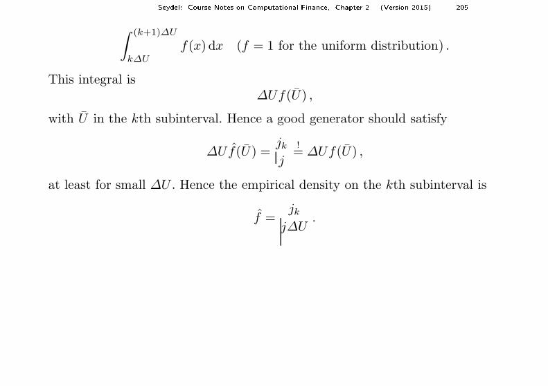
∫ (k+1)∆U

k∆U

f(x) dx (f = 1 for the uniform distribution) .

This integral is∆Uf(U) ,

with U in the kth subinterval. Hence a good generator should satisfy

∆Uf(U) =jk

j

!= ∆Uf(U) ,

at least for small ∆U . Hence the empirical density on the kth subinterval is

f =jk

j∆U.


Third requirement:

The lattice structure should be OK.To check this, arrange vectors out of mconsecutive numbers:

(Ui, Ui+1, . . . , Ui+m−1)

For U ∼ U [0, 1], these points should fill the m-dimensional unit-cube as uniformlyas possible. The sequences of points/vectors lie on (m − 1)-dimensional hyperplanes.Trivial case: M parallel planes through U = i

M , i = 0, . . . ,M − 1 (any one of the mcomponents).

A bad situation occurs when all points fall on only a few planes. Then the gapsbetween the planes without any points would be wide. This leads to analyze the latticestructure of the random points. The focus lies on the smallest number of planes, onwhich all points in [0, 1)m “land.”

Analysis for m = 2: In this planar case, the hyperplanes in (Ui−1, Ui)-space arestraight lines z0Ui−1 + z1Ui = λ, for parameters z0, z1, λ. From

Ni = (aNi−1 + b) mod M

= aNi−1 + b − kM for kM ≤ aNi−1 + b < (k + 1)M


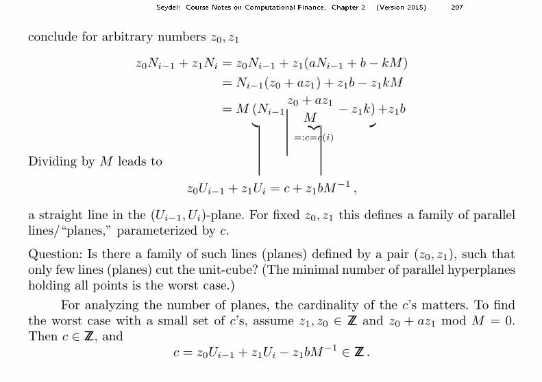
conclude for arbitrary numbers z0, z1

z0Ni−1 + z1Ni = z0Ni−1 + z1(aNi−1 + b − kM)

= Ni−1(z0 + az1) + z1b − z1kM

= M (Ni−1z0 + az1

M− z1k)

︸︷︷︸

=:c=c(i)

+z1b

Dividing by M leads to

z0Ui−1 + z1Ui = c + z1bM−1 ,

a straight line in the (Ui−1, Ui)-plane. For fixed z0, z1 this defines a family of parallellines/“planes,” parameterized by c.

Question: Is there a family of such lines (planes) defined by a pair (z0, z1), such thatonly few lines (planes) cut the unit-cube? (The minimal number of parallel hyperplanesholding all points is the worst case.)

For analyzing the number of planes, the cardinality of the c’s matters. To findthe worst case with a small set of c’s, assume z1, z0 ∈ ZZ and z0 + az1 mod M = 0.Then c ∈ ZZ, and

c = z0Ui−1 + z1Ui − z1bM−1 ∈ ZZ .


(z1bM−1 is a constant parallel shift not affecting the number of planes.) How many

of such c’s exist? For 0 ≤ U < 1 obtain a range for the c’s by a maximal set Ic ⊂ ZZ,such that

c ∈ Ic ⇒ the line touches or cuts the unit-cube .

The cardinality of the set Ic gives a clue on the distance between the parallel lines(planes). It is unfavorable when the set consists of only a few elements.

Academic Example Ni = 2Ni−1 mod 11 (i.e. a = 2, b = 0, M = 11)

The pair (z0, z1) = (−2, 1) solves z0 + az1 = 0 mod M .

Hence −2Ui−1 + Ui = c .

0

0.2

0.4

0.6

0.8

1

0 0.2 0.4 0.6 0.8 1

0 ≤ U < 1 implies −2 < c < 1.In view of c ∈ ZZ, the only parametersare c = −1 and c = 0. For this choice of (z0, z1)all 10 points in [0, 1)2 fall on only twostraight lines.

(0 does not occur for N0 6= 11k, k ∈ ZZ.) (Ui−1, Ui)-plane


Example Ni = (1229Ni−1 + 1) mod 2048

The condition z0 + az1 = 0 mod M

z0 + 1229z1

2048∈ ZZ

is satisfied by z0 = −1, z1 = 5, because

−1 + 1229 · 5 = 6144 = 3 · 2048 .

c = −Ui−1 + 5Ui − 52048 implies −1 − 5

2048 < c < 5 − 52048 . Hence the c’s consist

of only six values, c ∈ {−1, 0, 1, 2, 3, 4}, and all points in [0, 1)2 fall on six straightlines. — The Ui-distance between two neighboring lines is 1

z1

= 15 .

0

0.2

0.4

0.6

0.8

1

0 0.2 0.4 0.6 0.8 1

(Ui−1, Ui)-plane.In this figure,the discrete pointsare not separated.The sixth lineconsists of one point.


The (Ui−1, Ui)-points of these two examples are obviously not equidistributed. Thenext example is fine for m = 2 but shows that the good distribution for m = 2 doesnot carry over to higher m.

Example (RANDU)

Ni = aNi−1 mod M, with a = 216 + 3, M = 231

For m = 2 experiments show that the dots (Ui−1, Ui) are nicely equidistributed inthe unit square. For m = 3 it turns out that the random points in the cube [0, 1)3

fall on only 15 planes.

Analysis for larger m is analogous. (−→ Topic 14)


B. Fibonacci Generators

There are other classes of random-number generators, for example, the Fibonaccigenerators. A prototype of such generators is defined by

Ni+1 := Ni−ν − Ni−µ mod M

for suitable µ, ν (also with “+” or with more terms). Literature: [Knuth]

ExampleUi := Ui−17 − Ui−5,

in case Ui < 0 set Ui := Ui + 1.0

This is a simple example with reasonable features, but there are correlations.

The algorithm has a “leg” with length 17. This requires an initial phase that provides17 U -values to start the algorithm.


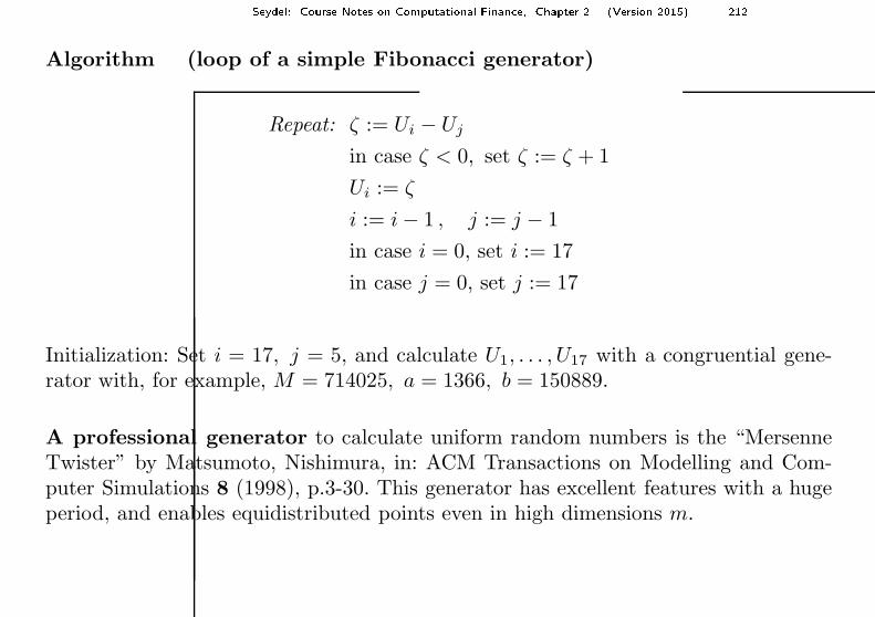
Algorithm (loop of a simple Fibonacci generator)

Repeat: ζ := Ui − Uj

in case ζ < 0, set ζ := ζ + 1

Ui := ζ

i := i − 1 , j := j − 1

in case i = 0, set i := 17

in case j = 0, set j := 17

Initialization: Set i = 17, j = 5, and calculate U1, . . . , U17 with a congruential gene-rator with, for example, M = 714025, a = 1366, b = 150889.

A professional generator to calculate uniform random numbers is the “MersenneTwister” by Matsumoto, Nishimura, in: ACM Transactions on Modelling and Com-puter Simulations 8 (1998), p.3-30. This generator has excellent features with a hugeperiod, and enables equidistributed points even in high dimensions m.


0.2

0.4

0.6

0.8

1

0 0.2 0.4 0.6 0.8 1

10000 random numbers(Ui−1, Ui), calculated witha Fibonacci Generator


2.2 Random Numbers from Other Distributions

The generation of all kind of deviates is based on uniform deviates. For the calculationof random numbers from a given distribution we can apply several methods, namely,inversion, transformations, and rejection methods.

A. Inversion

Let F (x) := P(X ≤ x) be a distribution function, for a random variable X, and P isthe corresponding probability.

Theorem (inversion)

Suppose U ∼ U [0, 1] and let F be a continuous strictly increasing distributionfunction. Then X := F−1(U) is a sample from F .

Proof:

U ∼ U [0, 1] means P(U ≤ ξ) = ξ for 0 ≤ ξ ≤ 1. Hence

P(F−1(U) ≤ x) = P(U ≤ F (x)) = F (x).


Application

Calculate u ∼ U [0, 1] and evaluate F−1(u). These numbers have the desired distri-bution. Mostly inversion is done numerically because F−1 in general is not knownanalytically.

There are two variants:

(a) F (x) = u is a nonlinear equation for x, which can be solved iteratively withstandard methods of numerical analysis (e.g. Newton method). For the normaldistribution (Figure) the iteration requires tricky termination criteria, becausefor u ≈ 0, u ≈ 1 small perturbations in u lead to large perturbations in x.

u=F(x)1/2

x

1

u

(b) Construct an approximating function G such that G(u) ≈ F−1(u). Then onlyx = G(u) needs to be evaluated. The construction of G must observe theasymptotic behavior, which amounts to the poles of G. For the standard normal


distribution the symmetry w.r.t. (x, u) = (0, 12) can be exploited and only the

pole for u = 1 needs to be observed. This can be done with a rational functionG(u), with a denominator having a zero at u = 1.

B. Transformation

We begin with the scalar case: Let X be a random variable. What is the distributionof a transformed h(X)?

Theorem (scalar transformation)

Suppose X is a random variable with density function f and distribution functionF . Further assume

h : S → B

with S,B ⊆ IR, where S is the support of f , and let h be strictly monotonic.

(a) Y := h(X) is random variable with distribution function

F (h−1(y)) for increasing h

1 − F (h−1(y)) for decreasing h


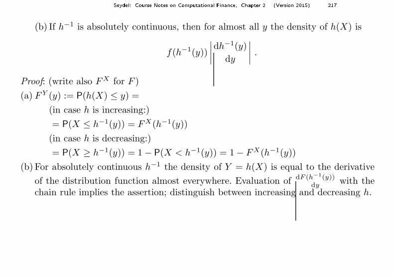
(b) If h−1 is absolutely continuous, then for almost all y the density of h(X) is

f(h−1(y))

∣∣∣∣

dh−1(y)

dy

∣∣∣∣.

Proof: (write also F X for F )

(a) F Y (y) := P(h(X) ≤ y) =

(in case h is increasing:)

= P(X ≤ h−1(y)) = F X(h−1(y))

(in case h is decreasing:)

= P(X ≥ h−1(y)) = 1 − P(X < h−1(y)) = 1 − F X(h−1(y))

(b) For absolutely continuous h−1 the density of Y = h(X) is equal to the derivative

of the distribution function almost everywhere. Evaluation of dF (h−1(y))dy with the

chain rule implies the assertion; distinguish between increasing and decreasing h.


Application

Start with X ∼ U [0, 1] and the density of the uniform distribution,

f(x) =

{

1 for 0 ≤ x ≤ 1

0 elsewhere

i.e. S = [0, 1]. Random numbers Y with prescribed target density g(y) are to becalculated. Hence we require a transformation h such that

f(h−1(y))

∣∣∣∣

dh−1(y)

dy

∣∣∣∣= 1

∣∣∣∣

dh−1(y)

dy

∣∣∣∣

!= g(y) .

Then h(X) is distributed as intended.

Example (exponential distribution)

The exponential distribution with parameter λ > 0 has the density

g(y) =

{

λe−λy for y ≥ 0

0 for y < 0.

B consists of the non-negative real numbers. As transformation [0, 1] → B wechoose the monotonic decreasing function


y = h(x) := − 1

λlog x

with inverse h−1(y) = e−λy for y ≥ 0. Since

f(h−1(y))

∣∣∣∣

dh−1(y)

dy

∣∣∣∣= 1 ·

∣∣(−λ)e−λy

∣∣ = λe−λy = g(y) ,

h(X) is distributed exponentially as long as X ∼ U [0, 1].

Application

Calculate U1, U2, . . . ∼ U [0, 1]. Then

− 1

λlog(U1), − 1

λlog(U2), ... are distributed exponentially.

(Hint: The distances between jump times of Poisson processes are distributed expo-nentially.)

Attempt with the normal distribution: Search for h such that

1 ·∣∣∣∣

dh−1(y)

dy

∣∣∣∣=

1√2π

exp

(

−1

2y2

)

.

This is a differential equation for h−1 without analytic solution. In this situation themultidimensional version of the transformation helps.


Theorem (transformation in IRn)

Suppose X is a random variable in IRn with density f(x) > 0 on the supportS. Let the transformation h : S → B, S,B ⊆ IRn be invertible and the inversecontinuously differentiable on B. Then Y := h(X) has the density

f(h−1(y))

∣∣∣∣

∂(x1, . . . , xn)

∂(y1, . . . , yn)

∣∣∣∣, y ∈ B, (2.7)

where ∂(x1,...,xn)∂(y1,...,yn) denotes the determinant of the Jacobian matrix of h−1(y).

Proof: see Theorem 4.2 in [L.Devroye: Non-Uniform Random Variate Generation(1986)]

In Section 2.3 the two-dimensional version will be applied to calculate normal variates.


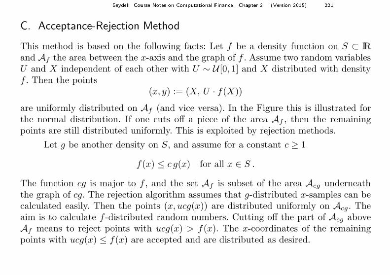
C. Acceptance-Rejection Method

This method is based on the following facts: Let f be a density function on S ⊂ IRand Af the area between the x-axis and the graph of f . Assume two random variablesU and X independent of each other with U ∼ U [0, 1] and X distributed with densityf . Then the points

(x, y) := (X, U · f(X))

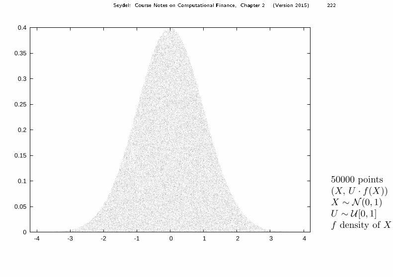
are uniformly distributed on Af (and vice versa). In the Figure this is illustrated forthe normal distribution. If one cuts off a piece of the area Af , then the remainingpoints are still distributed uniformly. This is exploited by rejection methods.

Let g be another density on S, and assume for a constant c ≥ 1

f(x) ≤ c g(x) for all x ∈ S .

The function cg is major to f , and the set Af is subset of the area Acg underneaththe graph of cg. The rejection algorithm assumes that g-distributed x-samples can becalculated easily. Then the points (x, ucg(x)) are distributed uniformly on Acg. Theaim is to calculate f -distributed random numbers. Cutting off the part of Acg aboveAf means to reject points with ucg(x) > f(x). The x-coordinates of the remainingpoints with ucg(x) ≤ f(x) are accepted and are distributed as desired.

Seydel: Course Notes on Computational Finan e, Chapter 2 (Version 2015) 222 0

0.05

0.1

0.15

0.2

0.25

0.3

0.35

0.4

-4 -3 -2 -1 0 1 2 3 4

50000 points(X, U · f(X))X ∼ N (0, 1)U ∼ U [0, 1]f density of X


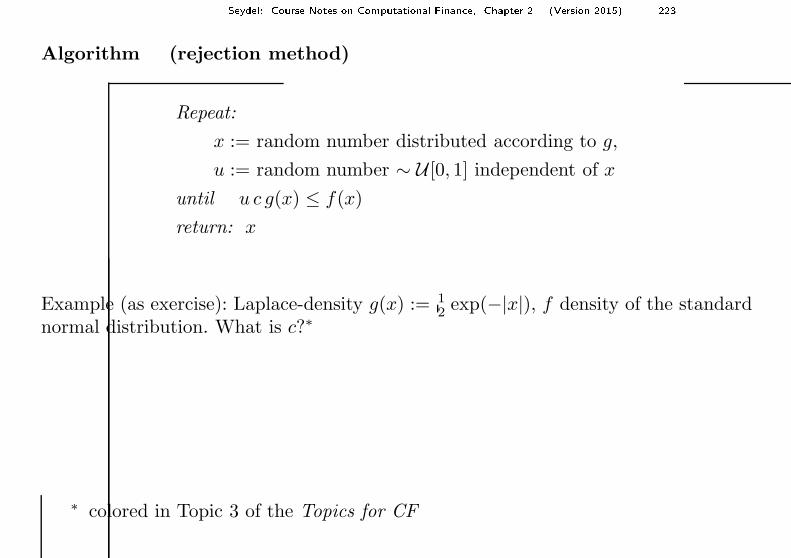
Algorithm (rejection method)

Repeat:

x := random number distributed according to g,

u := random number ∼ U [0, 1] independent of x

until u c g(x) ≤ f(x)

return: x

Example (as exercise): Laplace-density g(x) := 12 exp(−|x|), f density of the standard

normal distribution. What is c?∗

∗ colored in Topic 3 of the Topics for CF


2.3 Normal Deviates

This section applies the transformation theorem in IR2 to the calculation of normallydistributed random numbers, and sketches the ziggurat method.

A. Method of Box and Muller

S := [0, 1]2, X distributed normally on S with density f = 1 on S. Transformation h:{

y1 =√

−2 log x1 cos 2πx2 =: h1(x1, x2)

y2 =√

−2 log x1 sin 2πx2 =: h2(x1, x2)

inverse h−1:

x1 = exp{−1

2 (y21 + y2

2)}

x2 =1

2πarctan

y2

y1

For this transformation the determinant is

∂(x1, x2)

∂(y1, y2)= det

( ∂x1

∂y1

∂x1

∂y2

∂x2

∂y1

∂x2

∂y2

)

=

= − 1

2πexp

{−1

2 (y21 + y2

2)}

.


Its absolute value is the density of the two-dimensional normal distribution. Since∣∣∣∣

∂(x1, x2)

∂(y1, y2)

∣∣∣∣=

[1√2π

exp(−1

2y21

)]

·[

1√2π

exp(−1

2y22

)]

,

the two-dimensional density is the product of the one-dimensional densities of thestandard normal distribution. As a consequence, the two components y1, y2 of thevector Y are independent.

Application

When the two components x1, x2 are distributed ∼ U [0, 1], then the transformationprovides two independent y1, y2 ∼ N (0, 1).

Algorithm (Box-Muller)

(1) generate U1 ∼ U [0, 1] and U2 ∼ U [0, 1].

(2) θ := 2πU2, ρ :=√−2 log U1

(3) Z1 := ρ cos θ is ∼ N (0, 1)

(same as Z2 := ρ sin θ).


B. Variant of Marsaglia

Prepare the input x1, x2 for the Box–Muller transformation such that trigonometricfunctions are avoided. From U ∼ U [0, 1] obtain V := 2U − 1 ∼ U [−1, 1]. Two suchnumbers V1, V2 define a point in IR2. Define the disk

D := {(V1, V2) : V 21 + V 2

2 < 1}.

Accept only those pairs (U1, U2) such that (V1, V2) ∈ D. These accepted points areuniformly distributed on D. Transformation to (radius)2 and normalized angle:

(x1

x2

)

=

(V 2

1 + V 22

12π arg (V1, V2)

)

.

These (x1, x2) are distributed uniformly in S (−→ exercise) and serve as input forBox&Muller. The advantage is:

cos(2πx2) =V1

√

V 21 + V 2

2

, sin(2πx2) =V2

√

V 21 + V 2

2


Algorithm (polar method)

(1) Repeat: generate U1, U2 ∼ U [0, 1];

V1 := 2U1 − 1, V2 := 2U2 − 1;

until w := V 21 + V 2

2 < 1.

(2) Z1 := V1

√

−2 log(w)/w is ∼ N (0, 1)

( as well as Z2 := V2

√

−2 log(w)/w ).

The probability of acceptance (w < 1) is the ratio of the areas π4

≈ 0.785....That is, 21% of all draws (U1, U2) are rejected. But these costs are compensated bythe saving of trigonometric functions, and Marsaglia’s polar method is more efficientthan standard Box&Muller.


C. Ziggurat Algorithm

A most efficient algorithm for the generation of normal deviates is the ziggurat algo-rithm, which is a acceptance-rejection method.

Essentially, g is a step function ≥ the Gaussian density f . Construction withN horizontal layers of N − 1 rectangles with the same area, and one bottom segmentwith the same area, which is no rectangle but infinite because of the tail of f . Thefigure illustrates schematically a situation for x ≥ 0, where the rectangle consists oftwo portions (for each i with 0 < i < N−1), which make an extremely efficient test foracceptance possible (random choice of the layer i; uniformly distributed test point).

xx i+1 ix

f(x)y

yi


2.4 Correlated Normal Random Variates

The aim is the generation of a normal random vector X = (X1, . . . ,Xn) with prescri-bed

µ = EX = (EX1, . . . ,EXn),

covariance matrix with elements

Σij = (CovX)ij := E ((Xi − µi)(Xj − µj)) ; σ2i = Σii

and correlations

ρij :=Σij

σiσj.

For the following assume that Σ is symmetric and positive definite.

Recall: The density function f(x1, . . . , xn) of N (µ,Σ) is

f(x) =1

(2π)n/2

1

(det Σ)1/2exp

{

−1

2(x − µ)trΣ−1(x − µ)

}

.


Assume Z ∼ N (0, I), where I is the unit matrix.

Apply a linear transformation x = Az, A ∈ IRn×n, where z is a realization of Zand A is nonsingular. Then

AZ ∼ N (0, AAtr)

This follows from the transformation theorem in Section 2.2B, with X = h(Z) := AZ.The density of X is

f(A−1x) |det(A−1)| =1

(2π)n/2exp

{

−1

2(A−1x)tr(A−1x)

}1

|det(A)|

=1

(2π)n/2

1

|det(A)| exp

{

−1

2xtr(AAtr)−1x

}

for arbitrary nonsingular matrices A. In case AAtr is a factorization of Σ, Σ = AAtr,and hence |det A| = (det Σ)1/2, we conclude:

AZ ∼ N (0, Σ) .

Translation with vector µ implies

µ + AZ ∼ N (µ,Σ) .

Example: Choose the Cholesky decomposition of Σ.Alternative: decomposition out of a principal component analysis.


Algorithm (correlated normal deviates)

(1) Decompose Σ into AAtr = Σ

(2) Draw Z ∼ N (0, I) componentwise

with Zi ∼ N (0, 1) for i = 1, ..., n, for example,

with Marsaglia’s polar method

(3) µ + AZ is distributed ∼ N (µ,Σ)

Example: If Σ =

(σ2

1 ρσ1σ2

ρσ1σ2 σ22

)

is required, the solution is

(σ1Z1

σ2ρ Z1 + σ2

√

1 − ρ2 Z2

)

.


2.5 Sequences of Numbers with Low Discrepancy

The aim is to construct points distributed similarly as random numbers, but avoid clus-tering or holes. In order to characterize equidistributedness, take any box (hyper-rectangle) in [0, 1]m, m ≥ 1. It would be desirable if for all Q

# of the xi ∈ Q

# all points in [0, 1]m≈ vol(Q)

vol([0, 1]m)

0

0.2

0.4

0.6

0.8

1

0 0.2 0.4 0.6 0.8 1

Q

For m = 2 the figure illustrates this idea in the unit square [0, 1]2.


Definition (discrepancy)

The discrepancy of a set {x1, . . . , xN} of N points xi ∈ [0, 1]m is

DN := supQ

∣∣∣∣

# of the xi ∈ Q

N− vol(Q)

∣∣∣∣.

We wish to find sequences of points, whose discrepancy DN for N → ∞ tends to zero“quickly.” To assess the decay we compare with the sequence

1√N

,

which characterizes the probabilistic error of Monte Carlo methods. For true randompoints the discrepancy has a similar order of magnitude, namely,

√

log log N

N.


Definition (sequence of low discrepancy)

A sequence of points x1, . . . , xN , . . . ∈ [0, 1]m is called low-discrepancy sequence ifthere is a constant Cm such that for all N

DN ≤ Cm(log N)m

N.

Comment

The denominator in 1N stands for relatively rapid decay of DN with the number of

points N , rapid as compared with the 1√N

of Monte Carlo.

But we have to observe the numerator (log N)m. Since log N grows only modestly,for low dimension m the decay of DN is much faster than the decay of the proba-bilistic Monte Carlo error.


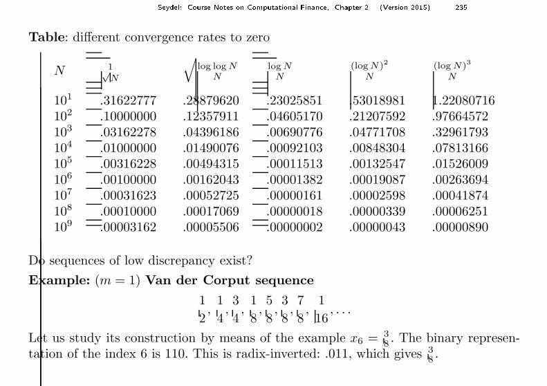
Table: different convergence rates to zero

N 1√N

√log log N

Nlog N

N(log N)2

N(log N)3

N

101 .31622777 .28879620 .23025851 .53018981 1.22080716102 .10000000 .12357911 .04605170 .21207592 .97664572103 .03162278 .04396186 .00690776 .04771708 .32961793104 .01000000 .01490076 .00092103 .00848304 .07813166105 .00316228 .00494315 .00011513 .00132547 .01526009106 .00100000 .00162043 .00001382 .00019087 .00263694107 .00031623 .00052725 .00000161 .00002598 .00041874108 .00010000 .00017069 .00000018 .00000339 .00006251109 .00003162 .00005506 .00000002 .00000043 .00000890

Do sequences of low discrepancy exist?

Example: (m = 1) Van der Corput sequence

1

2,

1

4,3

4,

1

8,5

8,3

8,7

8,

1

16, . . .

Let us study its construction by means of the example x6 = 38 . The binary represen-

tation of the index 6 is 110. This is radix-inverted: .011, which gives 38 .


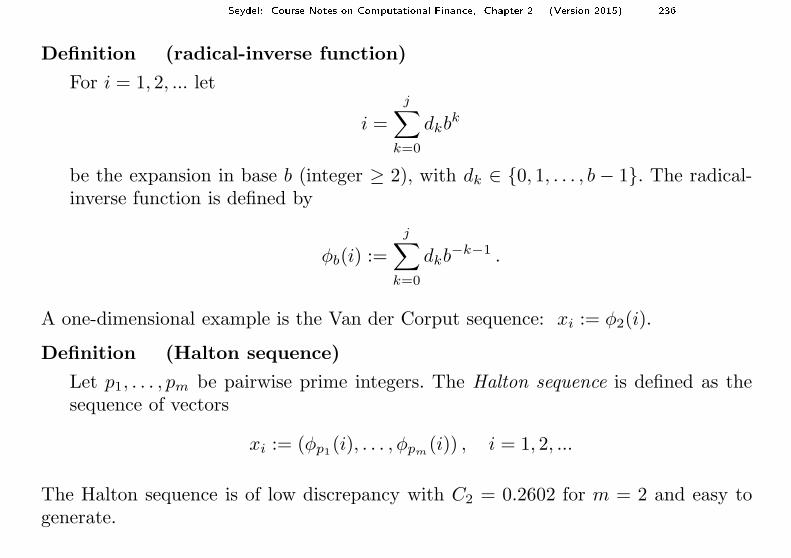
Definition (radical-inverse function)

For i = 1, 2, ... let

i =

j∑

k=0

dkbk

be the expansion in base b (integer ≥ 2), with dk ∈ {0, 1, . . . , b − 1}. The radical-inverse function is defined by

φb(i) :=

j∑

k=0

dkb−k−1 .

A one-dimensional example is the Van der Corput sequence: xi := φ2(i).

Definition (Halton sequence)

Let p1, . . . , pm be pairwise prime integers. The Halton sequence is defined as thesequence of vectors

xi := (φp1(i), . . . , φpm

(i)) , i = 1, 2, ...

The Halton sequence is of low discrepancy with C2 = 0.2602 for m = 2 and easy togenerate.


Other sequences of low discrepancy:

· Faure sequence

· Sobol sequence

· Niederreiter sequence

· Halton “leaped”: For large m the Halton sequence suffers from correlation. Thiscan be cured taking

xi := (φp1(li), . . . , φpm

(li)) , i = 1, 2, ...

for suitable prime l different from the pk, for example, l = 409.

The deterministic sequences of low discrepancy are called quasi-random numbers.(They are not random!)

Literature on quasi-random numbers: [H. Niederreiter: Random Number Generationand Quasi-Monte Carlo Methods (1992)]


0.2

0.4

0.6

0.8

1

0 0.2 0.4 0.6 0.8 1

The figure shows the first10000 Halton pointswith m = 2and p1 = 2, p2 = 3.

course notes on computational financeseydel/cfcoursenotes2beam.pdf · seydel: course notes on...

Documents