University of Nebraska - Lincoln University of Nebraska - Lincoln

DigitalCommons@University of Nebraska - Lincoln DigitalCommons@University of Nebraska - Lincoln

Dissertations and Theses in Agricultural Economics Agricultural Economics Department

Spring 5-2021

Corn Co-product Logistics – an Application of Linear Corn Co-product Logistics – an Application of Linear

Programming Programming

Dmitry Kalashnikov Adams University of Nebraska-Lincoln, dmitry.adams@adm.com

Follow this and additional works at: https://digitalcommons.unl.edu/agecondiss

Part of the Agricultural and Resource Economics Commons

Adams, Dmitry Kalashnikov, "Corn Co-product Logistics – an Application of Linear Programming" (2021). Dissertations and Theses in Agricultural Economics. 66. https://digitalcommons.unl.edu/agecondiss/66

This Article is brought to you for free and open access by the Agricultural Economics Department at DigitalCommons@University of Nebraska - Lincoln. It has been accepted for inclusion in Dissertations and Theses in Agricultural Economics by an authorized administrator of DigitalCommons@University of Nebraska - Lincoln.

CORN CO-PRODUCT LOGISTICS – AN APPLICATION OF LINEAR

PROGRAMMING

by

Dmitry Adams

A THESIS

Presented to the Faculty of

The Graduate College at the University of Nebraska

In Partial Fulfillment of Requirements

For the Degree of Master of Science

Major: Agricultural Economics

Under the Supervision of Professor Jeffrey R. Stokes

Lincoln, Nebraska

May 2021

CORN CO-PRODUCT LOGISTICS – AN APPLICATION OF LINEAR

PROGRAMMING

Dmitry Adams, M.S.

University of Nebraska 2021

Advisor: Jeffrey R. Stokes

This thesis applies the classic case of Linear Programing - the transportation problem - to optimize

corn co-product logistics between six ethanol producing facilities. The main purpose of this article

is the application of economic modeling and interpretation of the solution to aid in managing a real

world transportation network. An empirical application of the transportation problem is included

along with sensitivity analysis interpretation to illustrate the usefulness of the model in business

decision making. The concluding section presents an outlook for future expansion of the model to

include cost of inbound commodity and considerations of processing margins.

1

Table of Contents

Chapter 1: Examining a logistical problem and applying operations research principles to

develop a solution…………………………………………………………………………………1

1.1 Introduction….…………………………………………………………………………….1

1.2 Statement of the problem………………………………………………………………….9

1.3 Objective ………………………………………………………………………………...10

1.4 Methodology……………………………………………………………………………..11

1.4a General transportation problem model…..………………………………………...12

1.4b Case study and application of the model……..…………………………………….13

Chapter 2: Evaluating the results of linear programming model and interpreting the

sensitivity analysis to understand how that information could be used…………………......16

2.1 Results……………………………………………………………………………………16

2.2 Linear programming modeling for logistical disruptions……..…………………………17

2.3 Evaluating benefits of LP modeling relative to conventional logistics management…....19

2.4 Sensitivity analysis…….…………………………………………………………………21

2.5 Concluding remarks and outlook………...………………………………………………28

References………………………………………………………………………………………..30

Tables and Figures………………………………………………………………………………33

Appendix I…………………………………………………………………………………….…42

Appendix II...………………………………………………………………………………….…64

1

CHAPTER 1

1.1 Introduction

Mathematical research has made available a variety of tools which can be applied in

economics. One of those tools is linear programming (LP) which has proven useful in

practical applications and can aid in solving managerial problems. The purpose of this

research is not to explore the full potential or study the general field of linear programming.

Rather the focus is on applying a particular type of linear programming to a specific

problem. The type applied is a transportation problem, leading to the optimization of corn

germ transportation between six different ethanol plants.

The ethanol industry in the United States is complicated and requires large volumes

of inbound and outbound commodities to be synchronized with plant processing capacities

as well as inventory storage restrictions. Storage and processing capacity constraints make

transportation logistics an integral part of the process.

Although similar, the ethanol industry employs two main methods of corn

processing described as wet milling and dry milling. The dry milling process refers to a

method where a whole corn kernel goes through a set of rollers “dry” (typically15 percent

moisture content), and is then sent to fermentation tanks to be made into ethanol and several

other corn co-products, mainly dried distiller grains (DDGs). While the wet milling process

is also mechanical, one of the key differences of the process is the separation of the corn

kernel through a series of steps. The first step is steeping or soaking of the corn, thus the

name wet mill. This step is used to separate the corn into four different components: starch,

gluten, hull, and germ. Starch gets used to make alcohol or ethanol, corn sweeteners, or is

shipped out as a co-product to be processed further into a wide variety of consumer

2

products. Gluten and hulls get blended into animal feed products or sold to end users as

feed ingredients. Corn germ is further processed or spun into corn oil and corn germ meal.

In some instances, it is necessary to transport corn germ to different facilities due to some

wet mills not having the necessary equipment to process corn germ or lack the capacity to

process all of their own supply. Furthermore, majority of processing plants in the industry

will operate around the clock which often results in processing equipment failure due to

missed maintenance. Various other factors could also force a corn processing plant to ship

corn germ which makes optimized outbound logistics an integral step in achieving overall

corn processing efficiency.

Throughout this study six different ethanol plants shown in Figure 1 are considered.

All six facilities utilize a wet milling process which will produce corn germ with varying

daily yields due to grain quality, various equipment differences, the size and speed of

processing, etc. However, for the purpose of this model, using an average yield of 3.2 lbs.

per bushel of corn will be more practical. A key distinction between these ethanol facilities

is their capacity to process and store corn germ on site. The six facilities are: 1) ADM

Columbus, NE 2) ADM Marshall, MN 3) ADM Clinton, IA 4) ADM Cedar Rapids, IA 5)

ADM Decatur, IL and 6) Cargill Blair, NE. Only three out of the six facilities mentioned

above have the necessary equipment to process corn germ: 1) Cargill in Blair, NE 2) ADM

in Clinton, IA 3) ADM in Decatur, IL. The processing capacity is different at each facility

and is a function of storage space for inbound material, the number of product receiving

bays, and the capacity of corn germ processing equipment.

At the moment, from ADM’s perspective, there is no system in place that would

aid in logistics management. Although it is possible to operate a network intuitively and

3

over time for a particular manager to gain efficiencies. However, management of such

complex problem by intuitive or observational analysis of the situation which is dependent

on subjective evaluation could be prone to inefficiencies. The weak point of such a method

is that it does not approach the problem in a systematic manner and does little to improve

or advance the managerial decision process. Longer term, it is beneficial to employ a data

driven decision making approach.

The lack of consistent strategy behind corn germ logistics is the motivation behind

this empirical study where procedures developed by the Management Science/Operations

Research discipline will be employed to develop a linear transportation model. The

developed model will assist transportation network managers in making decisions to ensure

that an optimal solution is being considered.

The idea of viewing a problem from a company-wide perspective is described by

Cook and Russell (1985) as essential. In their view, “the good of the whole may not

necessarily derive from the greatest good for each of the parts. Concentrating only on a

particular component of the organizational system may result in optimization of that

component but less than optimal solution for the organization as a whole”. This statement

may seem counter intuitive, but the results of solving a few transportation network

problems by applying this methodology make it clear why this statement it true.

In many cases, sub-optimization of various components will be necessary to

accomplish the organization's goal of creating system-wide efficiency. The Operations

Research/Management Science (OR/MS) systems approach equips the decision makers

with the ability to determine which alternative will realize the organization’s goal. Besides

finding an optimal and the most cost-effective solution, the advantages of the systems

4

approach is that it allows for the optimization of an organization’s overall goals and not

just those of isolated departments or components of the system.

Applying an OR/MS approach, a manager will be able to determine the optimal

solution and interpret the shadow costs of operating corn germ logistics in a way that may

not be as efficient. Understanding shadow cost will enable logistics managers to determine

the limit of adjusting freight rates to coordinate with other divisions to gain an advantage

over competitors.

At the core of OR/MS is the use of scientific method of decision making. OR/MS

approaches provide a rational, systematic way to handle complex problems. However, it

should be noted that while the linear programming model will always provide a theoretical

optimal solution, that solution may not always be perfectly implemented in practice.

Various subjective obstacles may inevitably arise in real-world application of the model.

Employing a structured approach, the decision maker has a better chance to make a proper

judgment. A systematic approach will provide some key insights about the problem that

would otherwise seem obscure (Cook & Russell). The purpose of this research will be to

provide an example of how linear programming can be applied in the industry and point

out benefits of using a system-wide approach versus conventional methods. The focus of

the research is on the transportation of corn germ between processing facilities.

One specific case of linear programing is the transportation problem (TP) that was

first studied by Leonid Kantorovich who at the time, had an international reputation for his

creative work in pure and applied mathematics. Kantorovich was the first to apply linear

programming to industrial production problems. While he was still a professor of

mathematics at Leningrad University in 1938, he was approached by a plywood

5

manufacturer with an optimization problem. The question seemed simple, maximize the

total output of five varieties of plywood by optimizing a work schedule of eight lathes that

had different output capacities, subject to constraints of a particular product output

combination. However, at the time, empirical application of solving this linear

programming problem seemed impractical (Kantorovich 1962) because of an immense

amount of time it would take to solve all possible combinations by hand.

Faced with what is now known as “The plywood trust problem,” Kantorovich

quickly classified this problem as belonging to a wide class of extremal problems with

linear constraints. The formulation of these problems is simple, but conventional practical

application would have been “utterly inapplicable since it requires the solution of tens of

thousands if not millions of systems of simultaneous equations” (Kantorovich 1940). It is

by encountering this problem, Kantorovich discovered an alternative way for solving linear

problems by “solving multipliers”. This discovery gave rise to a new branch of

mathematical economics and applied mathematics. Kantorovich later expanded the scope

of the theory from micro to macro applications of optimal planning and control of Soviet

planned economy encompassing: price discovery, theory of rent, efficiency of invested

capital (Kantorovich 1949). However, discovery is not an innovation until it is widely

accepted, shared, and applied. The adoption period of linear programing turned out to be

abnormally long. Kantorovich’s work was not recognized until the late 1950’s when his

work was published in a book Best Utilization of Economic Resources (Kantorovich 1960).

At the same time, in 1947, Dantzing, Wood, and Koopmans were working on a

similar method for solving complex problems. They independently discovered, developed,

and coined the discipline as linear programing in the United States. The discipline had the

6

potential for broad applicability to problems involving optimal choice of multiple resources

constrained by a set of constraints, similar to Kantorovich’s discovery. The practical

application of linear programming equally failed to take hold and was not widely adopted

in business applications until computer hardware and software made implementation of

linear programing computationally possible and more user friendly.

The classical transportation problem is a special case of linear programming. It is a

problem in which the single objective is to minimize the cost of transportation. The solution

provides an optimal amount of units to be shipped from a set number of origins, to a set

number of destinations satisfying supply, and demand constraints of the problem. Over

time, researchers have expanded on the classic transportation problem and developed

variations that consider the cost of goods shipped, seller profit, multiple-objective models,

time constraints, etc. (Roy, and Maity 2017).

The solution to bi-criteria transportation problems was developed by Aneya and

Nair (1979). Unlike the classical transportation problem, the bi-criteria formulation can

handle multiple key objectives simultaneously. This approach becomes very relevant in

perishable goods transportation problems when the objective is to minimize the total cost,

reduce the total transportation time, and preserve the quality of transported goods.

Although this problem is solvable by a conventional transportation problem formulation

where each objective can be optimized separately, it is not the most efficient way due to

computational complexity. By handling each objective separately, each solution will find

a set of non-dominant extreme points in the solution space, which then would require

additional manipulation to identify the optimal solution. The bi-criteria method will find

non-dominated extreme points in the criteria space and only uses these points to provide a

7

solution for implementation. Although this method was developed to solve transportation

problems with multiple objective functions, it is also an approach used to solve problems

involving production bottlenecks.

Prakash (1981) developed a method for solving a transportation problem with an

objective that minimizes transportation cost while minimizing the duration of transport

when the demand and supply quantities are unknown. This approach is based on a multi

objective linear programming method with imprecise parameters. An example of where

such an approach would be useful is in the package delivery industry where the number of

packages or goods to be shipped varies, but the duration of the shipment is fixed.

Another interesting take on solving linear programming was proposed by Chang

(2008) who developed a solution to a transportation problem that involved several choices

associated with parameters such as cost, supply, or demand. These options would make the

proper choice of parameters unclear for the decision maker.

A variation on a multi-choice objective transportation problem has also been

studied and includes a stochastic aspect (Roy et al. 2013). Here researchers consider

exponential distribution of all constraining parameters. The multi-choice stochastic

transportation problem is transformed into a deterministic model allowing for manipulation

of coefficients in the multi-choice objective function to become restricted binary variables.

These additional restrictions are dependent on the accuracy level associated with each cost

coefficient model. Some specific probabilities are also transformed into deterministic

constraints using a stochastic approach. This work was later expanded by Mahaptra et al.

(2013) and Roy et. al. (2014) in a study where supply and demand constraint parameters

8

follow a Weibull distribution and cost coefficients of the objective function are multi-

choice.

Although many different variations of the transportation problem model have been

developed and are useful for many types of real-world applications with single or multi-

objectives, unspecified supply or demand, or random location scheduling, for the case of

corn germ transportation, a classic transportation problem approach is most appropriate.

All of the constraining parameters in the model such as transportation costs and supply and

demand of the commodity are linear and set by the capacity of each processing plant. The

quantity of tons shipped from certain origin to a particular destination are the only

variables. Rather than developing a new way to expand on the classic transportation

problem model, which would include all possible variables pertaining to this specific case,

a quick and simple way to determine the optimized solution to minimize the cost of

transportation throughout the whole system would be most useful. The three focus areas of

this research will be on:

• Empirical application of the transportation problem model

• Interpretation of the solution and evaluation of sensitivity analysis

• Understanding and interpretation of shadow prices to aid in negotiation of

transportation rates and cost benefit analysis of processing capacity

expansion

The remainder of the thesis is organized as follows: Section 1.2 describes the germ

transportation problem. Section 1.3 will focus on the objective of the study. In section 1.4

the focus is on mathematical model with two subsections 1.4a and 1.4b. Subsection 1.4a

will describe a general case of a transportation problem model, while subsection 1.4b will

9

apply the model to this particular case of corn germ transportation optimization. Chapter

two will start with discussion of the model results in section 2.1 and will further expand on

the sensitivity analysis of the results in section 2.4. Section 2.2 will discuss the benefits of

using linear programing to optimize the network when logistical disruptions occur. In

section 2.3 actual freight expenditure incurred by ADM in 2019 is used as a benchmark

and compared with the optimized scenario using the Linear Programming model. The

concluding section 2.5 will summarize the application of the linear programming model

and future areas where this model could be expanded.

1.2 Statement of the problem

At the core, the problem of corn germ logistics lies in transporting products from areas of

excess supply to areas with excess demand. The challenge of optimizing corn germ

logistics lies in managing transportation between producing facilities that do not have their

own processing capacity and must ship corn germ to a facility that has excess capacity by

utilizing either rail or truck method of transportation. This must be done in a manner where

none of the processing facilities get overwhelmed by inbound corn germ as well as

producing facilities being able to ship all of their daily corn germ production. This

transportation problem also involves two separate companies, ADM and Cargill, and it

needs to consider an agreement between the two in the form of a constraint.

The constraint is represented as a corn germ processing capacity exchange between

ADM Decatur and Cargill Blair. It is based on a beneficial relationship between processing

facilities that produce corn germ in different geographic locations (see Figure 1) and lack

processing capacity on site. Nearby competitor facilities, however, have surplus capacity

to process corn germ. ADM Columbus processing plant is lacking capacity to process corn

10

germ and Cargill Blair has excess processing capacity. Similarly, a Cargill processing plant

in Dayton, OH lacks capacity to process all its corn germ supply and ADM Decatur has

surplus processing capacity. The quantity shipped from ADM Columbus to Cargill Blair

needs to equal the quantity shipped from Cargill Dayton to ADM Blair.

The primary objective of this research is to determine whether an OR/MS logistics

management approach could better optimize the transportation network. The objective of

the transportation model is to minimize the cost of corn germ transportation between

processing facilities. The process is complex due to multiple variables and constraints

which must be considered. For this model to be useful in helping to make management

decisions, a delicate balance between accuracy and simplicity must be found. The model

must be detailed enough to represent the essential realities of the problem and yet be

manageable in terms of computations, implementation, and solution execution.

The model formulation will be based on Applied Mathematical Programming using

algebraic systems. The most effective method for solving this linear programming problem

is the Simplex Method, which was developed by Dantzig and Wood (1947), Koopmans

(1951). A simplified and user-friendly model will be set up in excel based on the underlying

principles of the Simplex Method to solve linear programming problems.

1.3 Objective

The goal of this project is to develop a decision support system which will include a large-

scale linear programming model at its core. In other words, produce a linear programming

model that will aid in decision making of managing corn germ logistics in a systematic

way. This model will suggest an optimal mix of transportation methods and appropriate

tonnage amounts to be shipped out of each facility resulting in the most economical

11

transportation of corn germ system wide. Based upon set parameters, the decision support

system will output a series of descriptive reports which will illustrate the impact of

adopting a suggested solution. Sensitivity reports will enable users to assess the impact of

certain parameters changes, or shadow prices, without re-running the model. The

Operations Research/Management Science approach to corn germ logistics problem will

incorporate the following characteristics:

• Approaching a problem systematically

• Applying scientific methodology to develop a solution

• Using a system-wide or company-wide approach

• Formulate a mathematical model to represent actual company operations by means

of equations and other mathematical statements

• Analyze the results of the model within a formal framework and interpret the results

• Using computer software to run OR/MS model to accelerate the decision-making

process

With two modes of transportation between the facilities, rail and semi-truck, this linear

programming model will have fifteen decision variables, seven constraints, and will

incorporate logistics between six different corn processing plants located across the

Midwest. Shown in Figure 1 are the geographic locations of the ethanol facilities discussed

in this study.

1.4 Methodology

In a classical transportation problem, a typical objective is to minimize the total cost of

transportation throughout the entire system subject to demand and supply constraints. In

general form the transportation problem can be written as:

12

1.4a General TP Model

minimize:

𝑦 = ∑ ∑ ∁𝑖𝑗𝑥𝑖𝑗

𝑛

𝑗=1

𝑚

𝑖=1

subject to:

∑ 𝑥𝑖𝑗 ≥ 𝐷𝑗 (∀𝑗= 1, 2, … , 𝑛),

𝑚

𝑖=1

∑ 𝑥𝑖𝑗 ≤ 𝑆𝑖 (∀𝑖= 1, 2, … , 𝑚)

𝑛

𝑗=1

𝑥𝑖𝑗 ≥ 0 ∀ 𝑖 𝑎𝑛𝑑 𝑗

Where y is the total cost to be minimized, ∁𝑖𝑗(𝑖 = 1, 2, … , 𝑚; 𝑗 = 1, 2, … , 𝑛) is the unit

transportation cost of transporting a commodity from the 𝑖 th point of origin to 𝑗 th

destination and 𝑥𝑖𝑗 is the number of units shipped from 𝑖 th point of origin to 𝑗 th

destination. There are a total of m points of origin and n destinations. It must be noted that

𝑥𝑖𝑗 takes on a non-negative value because one cannot ship a negative number of units.

Supply, 𝑆𝑖 (𝑖 = 1, 2, … , 𝑚) and Demand, 𝐷𝑗 (𝑗 = 1, 2, … , 𝑛) as shown, are m points of

origin and hence, m supply constraints and n processing facilities and hence n demand

constraints at 𝑖th origin to 𝑗th destination. The constraints must guarantee that the demand

at each destination is satisfied, yet the quantity shipped must not exceed the supply

available. Therefore, ∑ 𝐷𝑥𝑖𝑗𝑚𝑖=1 ≤ ∑ 𝑆𝑥𝑖𝑗

𝑛𝑗=1 signifies that the supply must be at least

equal to or greater than demand, otherwise the problem will have no feasible solutions.

13

To solve the problem by hand, the most effective method will be the simplex

method. The simplex method is one of the most useful business applications of matrices to

solve simultaneous linear equations. The procedure is called Gaussian Elimination and is

a generalization of the simple elimination method for solving the 2 x 2 system see e.g.

(Cook, Russel 1985 pp. 720-726). There are many types of computer software available to

solve the problem and should be used to find the solution, therefore saving time.

1.4b Case study

Throughout this study six different ethanol plants will be considered. A standard industry

yield of 3.2lbs of corn germ per each bushel of corn (56lbs) processed will be used to set

up the problem. All six corn processing facilities utilize a wet milling process which will

produce corn germ with varying daily production shown in Table 2. The key distinction

between these ethanol facilities will be their capacity to process corn germ. Only three out

of six facilities have the necessary equipment to process corn germ: 1) Cargill in Blair,

NE 2) ADM in Clinton, IA 3) ADM in Decatur, NE. The processing capacity for each

facility is shown in Table 2. A flow diagram of corn germ between the six ethanol facilities,

utilizing two types of transportation methods, including rail and truck, with per unit cost

of each transport method is given in Figure 2. The methodology of how transportation

costs were calculated for each shipping lane are described in the Appendix sections.

The ethanol plants lacking corn germ processing capacity are denoted as 𝑖 ∈ 𝐼

from all possible points of origin 𝐼 (Columbus, Marshall, and Cedar Rapids), processing

plants with excess processing capacity are represented as 𝑗 ∈ 𝐽 to all possible

destinations 𝐽 (Blair, Clinton, and Decatur). Each transportation method will be denoted

as 𝑘 ∈ 𝐾 utilizing all possible modes of transportation 𝐾 (rail and truck) shown in Table

1. Further, let 𝑐𝑖𝑗𝑘 be the unit cost to ship from point of origin 𝑖 to destination 𝑗 via mode

14

𝑘 and 𝑥𝑖𝑗𝑘 be the quantity shipped from point of origin 𝑖 to destination 𝑗 via mode 𝑘. Let

𝑦 be the total shipping cost so that the mathematical model is formulated as follows:

minimize:

𝑦 = ∑ ∑ ∑ 𝑐𝑖𝑗𝑘 𝑥𝑖𝑗𝑘

𝑘∈𝐾𝑗∈𝐽𝑖∈𝐼

Naturally, the quantity available to be shipped depends on how much corn germ is

produced at each origin and the amount of corn germ needed at each destination. Let 𝑆𝑖

represent supply available to ship at each point of origin 𝑖 and 𝐷𝑗 represent the demand at

each destination 𝑗. This constraint is represented as follows:

∑ ∑ 𝑥𝑖𝑗𝑘

𝑘∈𝐾𝑗∈𝐽

= 𝑆𝑖∀ 𝑖

which indicates that total quantity shipped to all destinations via all modes of transportation

must equal the quantity available at each point of origin 𝑖 thus ensuring that all produced

corn germ is shipped (i.e., no product is stored at the origin). Similarly,

∑

𝑖∈𝐼

∑ 𝑥𝑖𝑗𝑘 ≤ 𝐷𝑗∀ 𝑗

𝑘∈𝐾

which indicates the total quantity shipped from all available origins 𝑖 via all available

modes of transportation 𝑘 cannot be larger than the processing capacity or demand at each

destination 𝑗. These constraints ensure that the processing capacity is not exceeded (i.e., no

product is stored at the destination). Additionally, the inability to ship corn germ to Cargill

Blair via rail is represented by the constraint

∑ 𝑥𝑖𝑗′𝑘′ = 0

𝑖∈𝐼

15

where 𝑗′ ∈ 𝐽 represents Cargill Blair and 𝑘′ ∈ 𝐾 represents rail transport. In this way, the

total quantity that can be shipped to Cargill Blair via rail is zero since all 𝑥𝑖𝑗𝑘 ≥ 0. Lastly,

due to the exchange arrangement between ADM and Cargill which specifies a certain

quantity that can be shipped to the Blair, NE processing plant, we represent the lower

(𝑥𝑚𝑖𝑛) and upper (𝑥𝑚𝑎𝑥 ) limits on the quantity of corn germ that can be shipped and

processed at Cargill Blair as follows:

𝑥𝑚𝑖𝑛 ≤ ∑ 𝑥𝑖𝑗′𝑘′′

𝑖∈𝐼

≤ 𝑥𝑚𝑎𝑥

where 𝑘′′ ∈ 𝐾 denotes truck transportation.

This model can be set up in this way and solved using “What’s Best” or “Solver” Excel

add-in computer software. This software will compute the most efficient combination of

transportation methods that satisfies all the constraints. The results of this problem will be

compared to transportation costs incurred by ADM in 2019, followed by a sensitivity

analysis discussion to show how the model results can be used in freight rate negotiation,

evaluation of capacity expansion or reduction, and estimation of alternative freight

combinations.

16

CHAPTER 2

2.1 Results

The solution to the case study shown in Table 11 reveals that the optimal transport method

combination heavily favors truck transportations, which is considerably different from the

current logistical plan at ADM that heavily relies on rail transportation. The results of the

linear programming model show that under normal operating conditions, 1,224 tons

(Columbus 280 tons, Marshall 288 tons, Cedar Rapids 656 tons) of corn germ should be

transported using semi-trucks and only 80 tons should be shipped using rail on a daily

basis.

Given the constraints of the receiving facilities seen in Table 3, Table 4 shows the

most cost-effective way to ship corn germ from ADM-Columbus ethanol plant is to

transport most of the product (280 tons) to Cargill in Blair, NE until constrained by the

daily limit set by the corn germ exchange agreement with Cargill. The remainder (80 tons)

of the production should be shipped to ADM in Clinton, IA via semi-truck. In total,

approximately 11 truckloads should be transported to Cargill in Blair, NE and roughly 3

truckloads should be shipped daily to ADM in Clinton, IA given normal operating

capacities. With this logistical combination, optimal transportation cost for ADM-

Columbus will amount to $5,815 daily (280 tons × $11 = $3,080 to ship germ to Blair via

truck plus 80 tons × $34.19 = $2,735 to ship germ to Clinton via truck).

17

As shown in Table 5, the model indicates that all 288 tons from ADM-Marshall

ethanol plant should be transported by semi-truck to ADM-Clinton. Which equates to about

12 daily truckloads and the optimal transportation expense for the ADM-Marshall plant

will amount to $11,534 daily.

As shown in Table 6, at ADM-Cedar Rapids, the most cost-effective method is to

transport all the product via semi-truck to ADM-Clinton which would amount to $7,216 in

daily expense to transport corn germ.

Under normal capacities and operating conditions, the total daily cost to transport

corn germ between all the facilities in the system would amount to $24,566. Under normal

operating circumstances, the results are straight forward and are not impossible to calculate

without the linear programming model. However, the model becomes increasingly

effective in providing the most cost-effective transportation combination when changes

occur anywhere in the transportation network as a result of logistical disruptions due to

adverse weather, processing capacity change due to equipment malfunctions, freight rates

increase due to market conditions, etc.

2.2 Linear program modeling for logistical disruptions

Consider the following scenario. At times during the winter, rail logistics get disrupted due

to adverse weather, which delays placement of rail cars at northern ethanol facilities. The

ethanol plant in Marshall, MN is particularly likely to experience rail logistics disruption,

which in turn, makes rail transportation unavailable for a period of time. Consider that at

the same time ADM-Clinton, IA experiences an equipment malfunction and loses some of

its processing, where the plant processing capacity is reduced to 900 tons of corn germ

daily instead of the normal 1,600 tons.

18

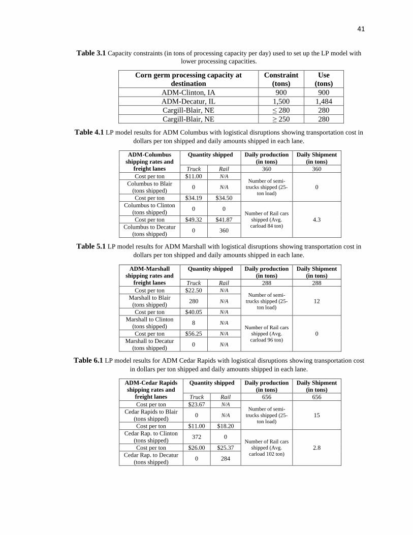
As shown in Table 3.1, processing constraints re-set for the new scenario with

reduced processing capacity at ADM-Clinton (only 900 tons) and no rail service at ADM-

Marshall. The developed LP model can now be used to determine the most cost-effective

way to manage corn germ logistics throughout the entire system. As show in Table 4.1, the

new results of the linear programming model indicate that for the ADM-Columbus ethanol

plant, the most efficient place to transport product now is via rail to Decatur, IL. This

creates a new transportation expense of $15,074 each day the logistical network is

disrupted. That is roughly a 160% increase or $9,260 in daily transportation expense for

that plant.

As shown in Table 5.1, the model indicates that the optimal logistical plan for

ADM-Marshall would be to ship 280 tons to Cargill-Blair via semi-truck. This constraint

is set by the ADM-Cargill agreement where Cargill-Blair would receive up to 280 tons of

corn germ daily from any origin within the ADM network. The remaining 8 tons should be

shipped to ADM-Clinton via truck. It is important to note that the remaining 8 tons of daily

production should not be shipped on a daily basis. Since the processing plant operates

around the clock, there is not a hard cut off on when the last ton of corn germ has to ship.

This is when the LP network management becomes more of an art rather than science and

this is when managerial decision making comes into play. Instead of only loading trucks to

a third of their capacity in the ADM-Marshall to ADM-Clinton truck lane, the operations

team could load that lane roughly every 3.25 days to stay consistent with the model and

avoid dead freight. Considering that nuance in network management, the total cost of this

logistical plan for ADM-Marshall plan would decrease by 43% and amount to $6,620 in

daily freight expense.

19

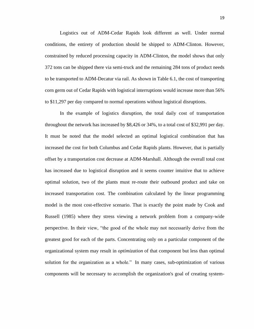
Logistics out of ADM-Cedar Rapids look different as well. Under normal

conditions, the entirety of production should be shipped to ADM-Clinton. However,

constrained by reduced processing capacity in ADM-Clinton, the model shows that only

372 tons can be shipped there via semi-truck and the remaining 284 tons of product needs

to be transported to ADM-Decatur via rail. As shown in Table 6.1, the cost of transporting

corn germ out of Cedar Rapids with logistical interruptions would increase more than 56%

to $11,297 per day compared to normal operations without logistical disruptions.

In the example of logistics disruption, the total daily cost of transportation

throughout the network has increased by $8,426 or 34%, to a total cost of $32,991 per day.

It must be noted that the model selected an optimal logistical combination that has

increased the cost for both Columbus and Cedar Rapids plants. However, that is partially

offset by a transportation cost decrease at ADM-Marshall. Although the overall total cost

has increased due to logistical disruption and it seems counter intuitive that to achieve

optimal solution, two of the plants must re-route their outbound product and take on

increased transportation cost. The combination calculated by the linear programming

model is the most cost-effective scenario. That is exactly the point made by Cook and

Russell (1985) where they stress viewing a network problem from a company-wide

perspective. In their view, “the good of the whole may not necessarily derive from the

greatest good for each of the parts. Concentrating only on a particular component of the

organizational system may result in optimization of that component but less than optimal

solution for the organization as a whole.” In many cases, sub-optimization of various

components will be necessary to accomplish the organization's goal of creating system-

20

wide efficiency. That exact point is illustrated in this scenario with disrupted logistics

where two of the facilities will sacrifice efficiency to achieve overall network efficiency.

Another scenario to consider is when facilities take scheduled downtimes. For

example if Cargill-Blair were to take their annual maintained downtime, that would

eliminate the possibility for ADM to ship corn germ to Cargill and forces ADM to keep

shipping within its own network. Furthermore, consider a scenario where at the same time

Cargill goes down for maintenance, market conditions for trucks cause the freight rates to

increase to a new average of $2.50/mile. With updated model constraints shown in Table

9.2 and increased truck freight costs shown in Table 10.2, the LP model quickly provides

a new logistics network combination.

With ADM-Columbus not being able to ship to Cargill-Blair, the LP model shown

in Table 13 provides the next optimal combination of shipping 136 tons of product to

ADM-Clinton and 224 tons of product to ADM-Decatur via rail. This disruption would

increase daily transportation cost by 142% or roughly $8,256 to a total of $14,070 for

ADM-Columbus.

ADM-Marshall would only be disrupted by higher truck freights and in this

scenario it would be more cost effective to send product by rail. The LP model suggest to

ship the entire daily production of 288 tons via rail to ADM-Clinton. The cost of

transportation increase by 9% or roughly $1,049 each day the truck freight rates were

elevated. The total transportation expense would increase to $12,583 each day.

ADM- Cedar rapids logistics would be unaffected by either of the disruptions and

the LP model suggests to continue shipping entire daily production to ADM-Clinton via

truck. Shown in Table 13, the total daily transportation expense with this shipping

21

combination would add up to $33,871 system wide. Although this daily cost of

transportation would increase by 37% or $9,306 per day higher compared to normal

operations, still this combination would be lower relative to typical alternative combination

determined by conventional network management. A typical conventional management

approach would focus on the cheapest method of transportation at each individual plant. In

the Columbus, NE plant, the entirety of ADM-Columbus production would rail to ADM-

Clinton (360 tons multiplied by $34.50) and leaving only 64 tons of available processing

capacity at ADM-Clinton. This would mean that ADM-Marshall had only ADM-Decatur

as the alternative destination to ship corn germ (288 tons multiplied by $57.35). Leaving

ADM-Cedar Rapids logistics unchanged, the total conventional approach would amount to

$36,150 in daily expenditure on transportation

This disruption in logistics and higher truck freight costs using LP approach would

amount to ADM-Columbus spending $12,419 and ADM-Marshall spending $16,515 per

day in transportation with ADM-Cedar Rapids unchanged. When compared the total cost

of transportation using conventional approach of $36,151 versus the LP model cost of

$33,871 the opportunity for cost reductions becomes clear. Although a 6% savings from

network efficiency is relatively small, over a two week disruption due to downtime, this

6% or $2,280 of daily efficiency could add up to $31,920 total transportation cost savings.

The same information could be extracted from the sensitivity analysis shown in

Table 10.2. Looking at row $C$50 and Reduced Cost column, we can see that forcing into

the model each additional unit shipped from ADM-Marshall to ADM-Decatur via rail

would increase the overall objective function by $6.2783 per unit shipped. Thus, if the

entire 288 tons were forced to be shipped to ADM-Decatur our objective function would

22

increase by $1,808.15 each day. Doing so would free up 288 tons of processing capacity at

ADM-Clinton, thus entire production from ADM-Columbus could be shipped to ADM-

Clinton leaving 64 tons of unused capacity (288 tons freed up capacity minus 224 tons of

product in Columbus plant switched destination from ADM-Decatur to ADM-Clinton).

Shown in row $C$28 and column Shadow Price in Table 9.2, those 64 tons of unused

capacity at ADM-Clinton would have a shadow price of $7.3755 per each unused unit.

Thus the total unused capacity at ADM-Clinton would add up to $472.03 ($7.3755 x 64

tons) and could be viewed as increased opportunity cost. Combined those two values would

add up to $2,280 ($472.03 opportunity cost plus $1,808.15 from forcing rail units to be

shipped to ADM-Decatur) total increase to the objective function.

These are just a few examples of how the linear programming models could be

used. In this industry, there could be a multitude of scenarios with logistical disruptions

and production constraints where the linear programming approach could be used

effectively for solving logistical problems. The benefit of solving logistical problems using

the linear programming method is saving time to find a solution and the confidence that

the new-found solution is the most cost-effective. One could also use the information that

the linear programming model provides to determine what it would cost to operate logistics

differently from the optimal combination by interpreting the sensitivity analysis and

observing shadow prices. This analysis will be discussed further in the Sensitivity Analysis

section. The Sensitivity Analysis section will point out the benefits of understanding the

marginal cost structure throughout the system and applying that knowledge to the logistics

planning purposes as well as going through an example of how that information could also

be used in freight rate negotiations.

23

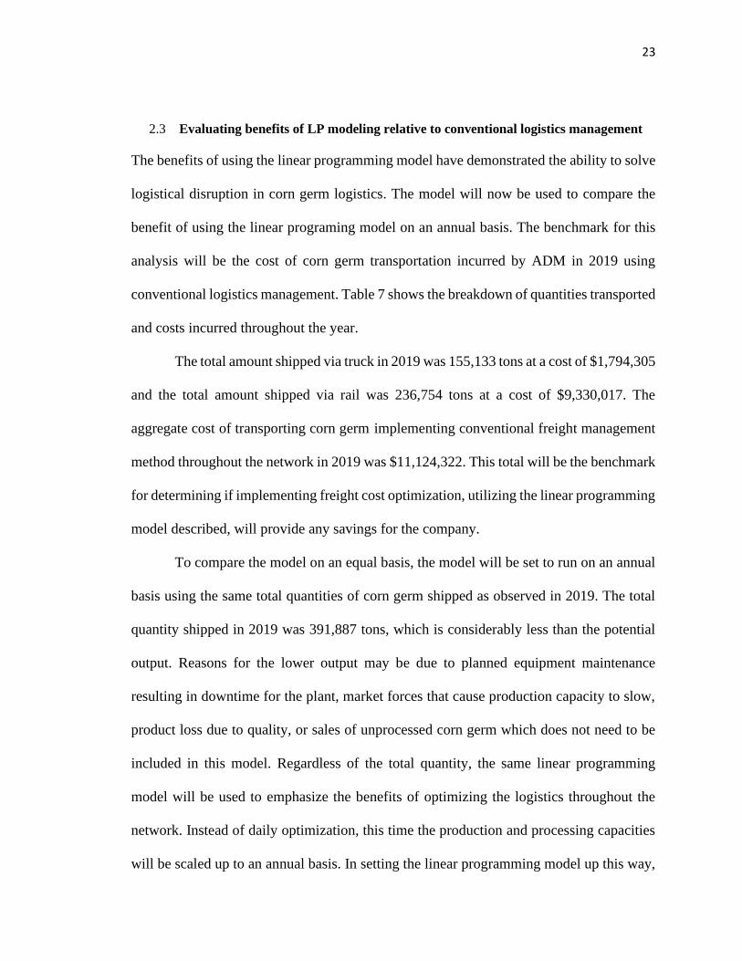
2.3 Evaluating benefits of LP modeling relative to conventional logistics management

The benefits of using the linear programming model have demonstrated the ability to solve

logistical disruption in corn germ logistics. The model will now be used to compare the

benefit of using the linear programing model on an annual basis. The benchmark for this

analysis will be the cost of corn germ transportation incurred by ADM in 2019 using

conventional logistics management. Table 7 shows the breakdown of quantities transported

and costs incurred throughout the year.

The total amount shipped via truck in 2019 was 155,133 tons at a cost of $1,794,305

and the total amount shipped via rail was 236,754 tons at a cost of $9,330,017. The

aggregate cost of transporting corn germ implementing conventional freight management

method throughout the network in 2019 was $11,124,322. This total will be the benchmark

for determining if implementing freight cost optimization, utilizing the linear programming

model described, will provide any savings for the company.

To compare the model on an equal basis, the model will be set to run on an annual

basis using the same total quantities of corn germ shipped as observed in 2019. The total

quantity shipped in 2019 was 391,887 tons, which is considerably less than the potential

output. Reasons for the lower output may be due to planned equipment maintenance

resulting in downtime for the plant, market forces that cause production capacity to slow,

product loss due to quality, or sales of unprocessed corn germ which does not need to be

included in this model. Regardless of the total quantity, the same linear programming

model will be used to emphasize the benefits of optimizing the logistics throughout the

network. Instead of daily optimization, this time the production and processing capacities

will be scaled up to an annual basis. In setting the linear programming model up this way,

24

the same logic applies, and results should illustrate potential benefits of optimizing the

network and reduce the transportation expense.

Table 8 shows the results for running the linear programming model on an annual

basis and transporting equivalent tonnages that were observed in 2019. The results of the

model show that there is clearly some room to capture savings. Although running the model

on an annual basis is oversimplified and does not include any logistical disruptions, it is

still possible to capture some of the difference in costs from using the LP modeling vs.

conventional freight management methods. By distributing truck tons throughout the

system, the total annual cost of corn germ logistics could be reduced to $7,757,681. That

is over $3.3 million in potential annual saving or 30 percent decrease in transportation cost

that does not require any capital investment. The reductions in transportation costs could

be captured simply through implementing linear program modeling throughout the network

in daily logistics management.

2.4 Sensitivity analysis

After observing the benefits of the model, consider the sensitivity analysis, where one can

use the information to understand the limits of cost structure without actually running the

program all over again. In this section a discussion will occur regarding the sensitivity

analysis of the two scenarios discussed in the previous section, one under normal operating

conditions and the second with logistical disruptions.

The sensitivity analysis is comprised of two sections, variable cells and constraints.

Shown in Table 9, under normal operating conditions one can observe the “Final Value”

versus the “R.H. Side Constraint” in the constraint section. The R.H. Side constraints are

values that were entered into the model which are based on actual plant processing capacity

25

and product storage limitations. Here one can see that 1,600 tons represents the daily

processing capacity in ADM-Clinton, 1,500 tons represent the capacity in ADM-Decatur

and so on. The Final Value is what the L.H Side equals after running the model, which

basically means how many variable units were used in each scenario. In this case, when

comparing the final value versus the constraint, one can see that most but not all the

processing capacity is used at ADM-Clinton. The constraint there is 1,600 tons per day and

the model is projecting that 1,544 tons of that capacity will be used. ADM-Decatur has

excess processing capacity as well and the LP model solution is only suggesting using 840

units out of the available 1,500, so those are non-binding constraints in this case. When

looking at the capacity in Cargill-Blair, the constraint is binding as the model uses all the

available 280 units that have been set as the R.H Side constraint.

The Allowable Decrease/Increase column and Shadow Price column must be

looked at together to understand the information presented by the sensitivity analyses. For

the first two rows, ADM-Clinton and ADM-Decatur, one can see that not all of the capacity

is used. The Allowable Decrease column is showing that the processing capacity can

decrease by 56 and 660 units at each plant respectively at a shadow price of zero. This

means that the final costs would not change if both of the R.H Side constraints were to

decrease by the allowable amount or that one can increase the amount of corn germ shipped

by 56 and 660 tons respectively. Therefore, it would not be necessary to re-run the model.

The interpretation is a bit more interesting when looking at the third row where the

constraint is set by Cargill-Blair. The allowable decrease of the R.H. side constrain in this

case is 30 units, which is set by the constraint in row $C$31, putting the minimum daily

shipment amount at 250 tons/day, at a shadow price of $23.19 per each unit. This means

26

that the final cost would increase by $23.19 for every unit capacity in Blair that is decreased

below 280 tons by the allowable decrease of 30 units. Likewise, the final cost would

decrease by $23.19 per each unit if the capacity in Blair were to increase by the allowable

80 units per day and can be interpreted as a cost that ADM should be willing to pay for

additional capacity. The shadow price of $23.19 is derived from the difference of the

cheapest method of transportation at ADM Columbus to Cargill Blair at $11/ton and the

second cheapest at ADM Columbus to ADM Clinton is $34.19. It is the marginal cost of

shipping corn germ to ADM Clinton above the constraining daily amount of 280 tons or it

could also be looked at as the marginal benefit of increasing capacity in Blair. Meaning

that if ADM were to pay Cargill $23.19 for each additional unit of capacity, up to the

allowable increase of 80 tons per day, the final cost of transporting corn germ would not

change.

An understanding of shadow prices becomes very valuable in negotiating because

a user can determine how the objective function changes when the variable units change

without re-running the model. In essence, a shadow price for each of the constraints shows

how much the objective function value will change for every unit change of a R.H. side.

While discussing processing capacity changes, any amount paid for increased capacity at

Cargill-Blair, less than the shadow price of $23.19, would be advantageous. In a scenario

where ADM Columbus were able to negotiate with Cargill to increase their daily capacity

in Blair by 80 units, up to a total 360 tons a day, for an agreement to pay anything less than

$23.19 per unit of that increased capacity. Then any difference below that amount would

be saved by ADM. For instance, if ADM were able to negotiate with Cargill and pay

$10/ton for an additional 80 tons of capacity per day in Blair, which would allow ADM to

27

ship a total of 360 tons daily, then the total cost of transporting corn germ would decrease

by the difference paid to Cargill. In this instance $10/ton, to increase their capacity and the

marginal cost ADM would have to otherwise pay to ship corn germ to Clinton at

$23.19/ton. In that scenario, ADM would be able to save $13.19/ton in marginal cost on

80 units per day, which would add up to savings of about $1,055 per day or roughly

$385,000 annually.

The same approach can be taken in determining whether to sell unprocessed corn

germ free on board (FOB) the plant where the buyer pays the cost to transport, or to keep

the corn germ in the ADM system and process it for a certain margin. To illustrate this,

consider an example where a buyer is willing to pick up all of the corn germ produced at

an ADM ethanol plant in Marshall, MN for $100/ton FOB the plant. At the same time, the

margin of processing the corn germ is only $30/ton. The merchandiser would be faced with

choosing the most valuable option, which could be difficult without knowing the

opportunity cost/shadow price or the exact amount that could be sold FOB or the amount

that could be shipped and proceed in order to optimize the network. Having the sensitivity

analysis provided by the optimal solution, the decision becomes very clear and easy to find.

Table 9 provides the user with the necessary information to make an appropriate decision.

The opportunity cost of processing or selling corn germ FOB the Marshall plant

can be found in Table 10 row $B$48 in reduced cost/shadow price column. The cost of

processing the corn germ would be -$10.05/ton per unit or $30/ton per unit of processing

margin minus $40.05/ton per each unit processed, versus $70/ton of each unit of

unprocessed corn germ sold FOB ADM Marshall ethanol plant or $100/ton paid by the

buyer FOB the plant minus $30/ton that could be gained by processing corn germ. A

28

decision to sell corn germ FOB Marshall plant would result in $10.05/ton up to 288 tons

of allowable decrease shown in row “$B$48”, column “Allowable Decrease” in Table 10.

Next, one can interpret the Final Value column which is the optimal unit value

chosen by the LP model. In this example that value represents the total tons shipped from

specific origin to a specific destination using a truck or rail mode of transportation. The

Reduced Cost column shows the shadow prices for the non-negativity constraint. This

value represents how much the objective function would change if one were to force a unit

into the model. For instance, consider the third row and reduced cost column in Table 10

and forced one additional unit into the model to be shipped from ADM-Columbus to ADM-

Decatur via truck, the objective function would increase by $15.13. That increase is the

difference in cost of freight from the next cheapest alternative method of transportation

which is ADM-Columbus to ADM-Clinton via truck. The Objective Value coefficients in

the model also have allowable increase and decrease, which reveals how much those values

could change without affecting the solution. In this example, the Objective Coefficient

values are the actual freight rates that were observed and used to set up this LP model.

Understanding what this information represents could become a powerful tool

when negotiating freight rates with truck carriers and rail roads as it shows exactly how

much a particular freight rate could be increased or decreased without changing the optimal

solution. Sensitivity analysis also shows how changing freight rates may or may not require

re-running the model. To illustrate this point, consider the values in row $B$38 in Table

10 where there is an option of shipping corn germ out of ADM-Columbus to ADM-Clinton

via truck or rail. Both freight rates are similar in value; however, rail freight rate is about

$.31/ton more expensive compared to the truck rate. If rail transportation is preferred, then

29

in order to keep total transportation cost optimized, one could approach the railroad with

this information and re-negotiate the rail freight rate $.31/ton lower to match the truck

freight rate. If negotiating rail freight is unsuccessful, then another way to lower the cost

of transportation per unit would be to find a way to increase the load amount per each rail

car. Increasing the loaded weight of each car shipped would increase efficiency and lower

the per unit cost of rail transportation.

Another useful way to use the information from the sensitivity analysis report is the

ability to quickly find the optimal destination to divert product when one of the facilities

goes off-line. Consider the previous example when ADM-Clinton lost 700 tons of their

corn germ processing capacity and was now only able to receive 900 tons per day (1,600

tons original capacity minus 700 tons hypothetical reduction). In this case, a logistics

manager would be faced with a choice to divert 644 tons of corn germ (700 tons reduction

minus the unused capacity of 56 tons) from ADM-Clinton to a different destination. The

Final Value column of Table 10 would have to be adjusted in a way that diverts 644 tons

from ADM Clinton in the most cost-effective way. To do that, one needs to identify where

the cheapest cost of switching is. This is a reasonably tedious task, but it could be solved

by comparing shadow prices in the Reduced Cost column in highlighted rows in Table 10.

In total one needs to find 644 tons in the network that could be diverted and the most

obvious place to start would be to look at the ADM-Marshall plant since all of their product

is currently being shipped to ADM-Clinton. By comparing shadow prices in the Reduced

Cost column for ADM-Marshall, the least expensive place to divert product would be to

Cargill-Blair. The 280 tons of germ should be rerouted to Cargill-Blair at an additional

$5.64 per ton in transportation expense.

30

It would be important to discuss where this additional cost of $5.64 comes from.

Simply put, Table 10 highlights Reduced Cost column which represents a cost increase in

the objective function from forcing each additional unit shipped by truck from Marshall to

Blair and would increase overall costs transportation by $5.64 each time a unit is added.

This happens because it also forces one less ton of product to be shipped from ADM-

Columbus to Cargill-Blair which would result in one more ton shipped from Columbus to

Clinton and one less ton shipped from Marshall to Clinton. That is the actual exchange

taking place. In other words, ADM-Columbus shipping costs increase by $34.19-

$11=$23.19 when ADM-Marshall shipping costs go down by $40.05-$22.5=$17.55. The

net change to the system is an increase of $23.19-$17.55=$5.64. All of this is within the

constraints of the originally modeled system and the shipment totals into Clinton and Blair

didn’t change which would satisfy the original capacity constraints. The new model, with

the smaller capacity at Clinton, would not actually allow this exchange to take place.

However, it would be the cost of forcing this diversion onto the original system. Hence, it

explains the increase in costs for the solution to the new system verses the old.

Following this principle, since the capacity at Cargill-Blair is maxed out from re-

routing product from ADM-Marshall, to solve the diversion problem one must look at

rerouting corn germ from ADM-Columbus. The least expensive way to accomplish that is

to divert product out of ADM-Columbus and ship it by rail to ADM-Decatur at an

additional $7.68 per ton shown in Table 10 highlighted Reduced Cost column. With a total

of 360 tons of product diverted, accounting for 56 tons of unused capacity in ADM-Clinton

from the original problem, that means that the total freed up capacity in ADM-Clinton is

now 416 tons. The only place left to divert product would be out of ADM Cedar Rapids,

31

which means that 284 tons of that plants production must be diverted elsewhere. The only

available plant with extra capacity left would be ADM-Decatur and the least expensive

alternative for ADM-Cedar Rapids plant is to use rail at an additional $14.37 per ton. In

total, the cost of diverting product due to reduced capacity in Clinton would increase the

transportation expense at the Columbus plant by $2,764 (360 tons diverted multiplied by

the shadow price $7.68/ton). The cost of diverting product out of the ADM-Marshall plant

would increase the objective function by $1,579 (280 tons diverted multiplied by shadow

price of $5.64 per ton). The transportation cost increase out of the Cedar Rapids plant

would be $4,081 (284 tons multiplied by shadow price of $14.37) and the system-wide

increase would amount to roughly $8,424 each day the logistics are disrupted.

It must be noted that the network diversion leaves an impression that the costs for

the ADM-Marshall plant went up by $1,579 which is incorrect. The objective function

increase by that amount, in other words, that is the total network costs increase and the

shipment costs from ADM-Marshall plant actually went down by $4,914. The real power

of linear programming is that it is able to move to the next cheapest way to handle the

shipments when the current way is no longer possible, even when many complicated swaps

are involved to achieve an optimal solution.

As shown in Table 9.1 and Table 10.1, the same analysis would be much quicker

and more precise by simply changing the fixed values/constraint to 900 tons of capacity at

ADM-Clinton to reflect reduction in processing capacity by 700 tons per day and then re-

run the LP model to come up with the same result. These results could be confirmed when

comparing the final value of our objective functions prior to diversion $24,564 shown in

Table 11 and the final value of $32,991 after the diversion shown in Table 12. The net

32

difference of the two scenarios is $8,427 which is a bit more precise figure then an estimate

made just by looking at the sensitivity report of the original problem. Although re-running

the LP model is more precise and much quicker, understanding and interpreting the

sensitivity analysis of the LP model is the key in getting a full picture of how different

elements of the model fit and work together to get a sense of direction. Rather than

thoughtlessly re-running the LP model to get a different result.

These are just a few examples of how the sensitivity analysis data could be used to

understand the interaction between individual variables and how constraints affect the

objective function of this LP model. There are virtually an unlimited number of

combinations how this model could be manipulated to optimize the logistics network.

OR/MS approach to solving logistical problems provides a rational, systematic way to

handle a complex transportation problem and the OR/MS key feature is the use of the

scientific method of decision making.

2.5 Concluding remarks and outlook

With all the potential uses and benefits of using the LP model to solve logistical problems,

it would be important to note that no model is perfect, and no model can truly embody the

situation it represents. The success of the model developed in this thesis does not solely

depend upon the scientific techniques used, but it also requires the user to understand the

limitations set by the assumptions in the model.

In some instances, linear programing is prone to formulations which are

oversimplified. In cases where data is not always available, costs are not linear, or

additional (unjustified by economic theory) constraints exist, the tendency is to use an

average or a representative value. Formulating a model in this way would mean that the

33

analysis will be attempting to estimate marginal reactions based on average data

observations and the resulting optimal solution will suffer from oversimplification.

However, another approach to set up the model containing nonlinear parameters is offered

by Richard E. Howitt. Howitt proposes to, “the majority of modelers who, for lack of an

empirical justification, data availability or cost, find that the empirical constraint set does

not reproduce the base-year results” a positive mathematical programming (PMP) method

for calibrating LP models with nonlinear elements (Howitt 1995). Howitt’s approach is

applied in three stages and will automatically calibrate the model using minimal data and

without using flexibility constraints. In this way Howitt emphasizes that problems

containing nonlinear elements such as crop yield variability, government policy,

technology, crop rotation, and other nonlinear constraints could be calibrated by applying

PMP methodology and will be more flexible in their response to changes in the model

parameters.

As the linear programming models become more sophisticated, a greater emphasis

should be placed on human factors. The LP model developed in this thesis will still require

a logistics manager to fill in with common sense in a case-by-case basis, always placing

the model at the foundation for any management strategy. Each model needs to achieve a

balance between purely quantitative approach, judgement, experience, and industry

insight. Utilizing the linear programming method to solve the logistical problems greatly

aids in decision making by expressing these problems as constrained linear models where

primary assumptions are: certainty of the parameters, linearity of the objective function

and the constraints in the model.

34

In this thesis the focus was to formulate a linear programming model which showed

some room for improvement in the ADM corn germ transportation network, but the real

power of the model lies in the ability to quickly adjust the recommended shipping logistics

if conditions change. Sensitivity analysis section emphasized usefulness of model solution

interpretation to future management decisions. Even though the LP model building is more

of an art than a science, any manager can gain competence through practice by formulating

models that solve their respective challenges. Model formulation is the one step that still

requires human insight of identifying the problem which is unable to be generated by a

computer.

35

References

Aneya Y.P. and K.P.K. Nair, Bi-criteria transportation Problem, Management Science (1979)

pp. 73-78

Cook, T., and R. Russell. 1985. Introduction to Management Science, 3rd. ed. New Jersey:

Prentice-Hall, Inc.

Chang C. T., Revised multi-choice goal programming, Applied Mathematical Modeling (2008)

pp. 2587-2595

Dantzig, G. B. 1949. Programming of inter-dependent activities II, mathematical model. Project

SCOOP Report Number 6, Headquarters, USAF, Washington, D.C. Also published in T. C.

Koopmans, ed. Activity Analysis of Production and Allocation. John Wiley and Sons, New

York, 1951, 19–32.

Google Maps, 2019. ARU: Saved Places in Google maps, 1:50. Google Maps [online] Available

through: ARU Library < https://www.google.com/maps/@42.1300335,-

94.9368726,7z/data=!4m3!11m2!2sUIQPlXaWppxcaRECeIFOUrkgRdfAnw!3e2>

[Accessed 15 April 2019].

Howitt R.E., Positive Mathematical Programming, American Journal of Agricultural Economics,

May, 1995, Vol. 77, No. 2 (May,1995), pp. 329-342

Kantorovich L.V., Mathematical methods of organizing and planning production, Management

Science (1960) 366-422.

Kantorovich L.V., Ekonomicheskii raschet nailychshego ispol’zovaniia resursov, Moscow: AN

SSSR. 2nd ed. (1960) pp. 338-353

36

Kantorovich L.V., Essays in Optimal Planning Bolshaya Sovetskaya Ensiclopedia. 3rd ed. Uspehi

matematicheskih nauk 1962 XVII Optimizatia

Kantorovich L.V., Selected Economic writings of L. V. Kantanovich, Ob odnom effectivnom

metode resheniia nekotorykh klassov ekstremalnykh problem, DAN SSSR Vol. 26 No. 3

1940 pp. 212-225

Kantorovich L.V., Selected Economic writings of L. V. Kantanovich, Podbor postavov

obespechivaiushchikh maksimal’nui vykhod produktsii pri zadannom assortimente,

Lishnaia Promyshlennost, No. 7 1949 pp.15-17 and No. 8 1949 pp. 17-19

Mahapatra D.R, S.K Roy and M.P. Biswal, Multi-choice stochastic transportation problem

involving extreme value distribution, Applied Mathematical Modeling (2013) pp. 2230-

2240

Pakash S., Transportation problem with objective to minimize total cost and duration of

transportation, Opsearch (1981) pp. 235-238

Roy S.K, D.R Mahapatra and M.P. Biswal, Multi-choice stochastic transportation problem with

exponential distribution, Journal of Uncertain Systems (2013) pp. 200-213

Roy S.K, Multi-choice stochastic transportation problem involving weibul distribution,

International Journal of Operational Research (2014) pp. 38-58

Roy S. K, G. Maity, Minimizing cost and time through single objective function in multi-choice

interval valued transportation problem, Journal of Intelligent & Fuzzy Systems 32 (2017)

1697-1709

37

Tables and Figures

Figure 1. Geographical locations of ethanol plants discussed in this article. (Google maps, 2019)

38

Figure 2. Flow diagram between 6 ethanol facilities and 15 transportation routes.

39

Table 1. Transportation cost (in dollars per ton) for transporting corn germ by truck or by rail

from origin i to destination j.

Blair, NE Clinton, IA Decatur, IL

Truck (𝑗1) Rail (𝑗2) Truck (𝑗3) Rail (𝑗4) Truck (𝑗5) Rail (𝑗6)

Columbus, NE (𝑖1) [11.00] [N/A] [34.19] [34.50] [49.32] [41.87]

Marshall, MN (𝑖2) [22.50] [N/A] [40.05] [43.69] [56.25] [57.35]

Cedar Rapids, IA (𝑖3) [23.67] [N/A] [11.00] [18.20] [26.00] [25.37]

Table 2. Showing daily corn germ production and corn germ processing capacity

Location Daily Corn Grind (in

bushels)

yield in

lbs/bu

Total daily

production

(tons)

Processing

capacity

tons/day

Columbus 225,000 3.2 360 N/A

Marshall 180,000 3.2 288 N/A

Clinton 325,000 3.2 520 1,600

Cedar Rapids 410,000 3.2 656 N/A

Decatur 525,000 3.2 840 1,500

Blair est. production* 190,000 3.2 304 250-280*

* Not a total corn germ processing. This processing capacity represents agreed upon processing

capacity exchange between ADM and Cargill

40

Table 3. Capacity constraints (in tons of processing capacity per day) used to set up the LP model.

Corn germ processing capacity at

destination

Constraint

(tons)

Use

(tons)

ADM-Clinton, IA 1,600 1,544

ADM-Decatur, IL 1,500 840

Cargill-Blair, NE ≤ 280 280

Cargill-Blair, NE ≥ 250 280

Table 4. LP model results for ADM Columbus showing transportation cost in dollars per ton shipped and

daily amounts shipped in each lane.

ADM-Columbus

shipping rates and

freight lanes

Quantity shipped Daily production

(in tons)

Daily Shipment

(in tons)

Truck Rail 360 360

Cost per ton $11.00 N/A Number of semi-

trucks shipped (25-ton load)

14 Columbus to Blair

(tons shipped) 280 N/A

Cost per ton $34.19 $35.59

Columbus to Clinton

(tons shipped) 80 0

Number of Rail cars

shipped (Avg.

carload 84 ton) 0 Cost per ton $49.32 $41.87

Columbus to Decatur

(tons shipped) 0 0

Table 5. LP model results for ADM Marshall showing transportation cost in dollars per ton shipped and

daily amounts shipped in each lane.

ADM-Marshall

shipping rates and

freight lanes

Quantity shipped Daily production

(in tons)

Daily Shipment

(in tons)

Truck Rail 288 288

Cost per ton $22.50 N/A Number of semi-

trucks shipped (25-ton load)

12 Marshall to Blair

(tons shipped) 0 N/A

Cost per ton $40.05 $59.05

Marshall to Clinton

(tons shipped) 288 0

Number of Rail cars shipped (Avg.

carload 96 ton) 0 Cost per ton $56.25 $64.68

Marshall to Decatur

(tons shipped) 0 0

Table 6. LP model results for ADM Cedar Rapids showing transportation cost in dollars per ton shipped

and daily amounts shipped in each lane.

ADM-Cedar Rapids

shipping rates and

freight lanes

Quantity shipped Daily production

(in tons)

Daily Shipment

(in tons)

Truck Rail 656 656

Cost per ton $23.67 N/A Number of semi-

trucks shipped (25-

ton load) 26

Cedar Rapids to Blair

(tons shipped) 0 N/A

Cost per ton $11.00 $19.73

Cedar Rap. to Clinton

(tons shipped) 656 0

Number of Rail cars

shipped (Avg. carload 102 ton)

0 Cost per ton $26 $27.60

Cedar Rap. to Decatur

(tons shipped) 0 0

41

Table 3.1 Capacity constraints (in tons of processing capacity per day) used to set up the LP model with

lower processing capacities.

Corn germ processing capacity at

destination

Constraint

(tons)

Use

(tons)

ADM-Clinton, IA 900 900

ADM-Decatur, IL 1,500 1,484

Cargill-Blair, NE ≤ 280 280

Cargill-Blair, NE ≥ 250 280

Table 4.1 LP model results for ADM Columbus with logistical disruptions showing transportation cost in

dollars per ton shipped and daily amounts shipped in each lane.

ADM-Columbus

shipping rates and

freight lanes

Quantity shipped Daily production

(in tons)

Daily Shipment

(in tons)

Truck Rail 360 360

Cost per ton $11.00 N/A Number of semi-

trucks shipped (25-

ton load) 0

Columbus to Blair

(tons shipped) 0 N/A

Cost per ton $34.19 $34.50

Columbus to Clinton

(tons shipped) 0 0

Number of Rail cars

shipped (Avg.

carload 84 ton) 4.3 Cost per ton $49.32 $41.87

Columbus to Decatur

(tons shipped) 0 360

Table 5.1 LP model results for ADM Marshall with logistical disruptions showing transportation cost in

dollars per ton shipped and daily amounts shipped in each lane.

ADM-Marshall

shipping rates and

freight lanes

Quantity shipped Daily production

(in tons)

Daily Shipment

(in tons)

Truck Rail 288 288

Cost per ton $22.50 N/A Number of semi-

trucks shipped (25-ton load)

12 Marshall to Blair

(tons shipped) 280 N/A

Cost per ton $40.05 N/A

Marshall to Clinton

(tons shipped) 8 N/A

Number of Rail cars shipped (Avg.

carload 96 ton) 0 Cost per ton $56.25 N/A

Marshall to Decatur

(tons shipped) 0 N/A

Table 6.1 LP model results for ADM Cedar Rapids with logistical disruptions showing transportation cost

in dollars per ton shipped and daily amounts shipped in each lane.

ADM-Cedar Rapids

shipping rates and

freight lanes

Quantity shipped Daily production

(in tons)

Daily Shipment

(in tons)

Truck Rail 656 656

Cost per ton $23.67 N/A Number of semi-

trucks shipped (25-

ton load) 15

Cedar Rapids to Blair

(tons shipped) 0 N/A

Cost per ton $11.00 $18.20

Cedar Rap. to Clinton

(tons shipped) 372 0

Number of Rail cars shipped (Avg.

carload 102 ton) 2.8 Cost per ton $26.00 $25.37

Cedar Rap. to Decatur

(tons shipped) 0 284

42

Table 7. The breakdown of all costs in a corn germ logistical network observed by ADM in 2019.

Corn germ

transported in 2019

Rail Quantity

in tons (billed

via RMS - Rail

Management

System)

Rail Freight

cost (using

tariff rate

with car

comp.)

Truck

Quantity in

tons (billed

via Agris)

Truck

Freight cost

(billed via

Agris)

Total tons

shipped

Total

transportatio

n cost (rail

and truck)

Columbus to Clinton 9,158 $315,923 1,239 $33,863 10,397 $349,786

Columbus to Decatur 73,160 $3,063,333 1,130 $38,614 74,290 $3,101,947

Columbus to Blair - - 52,044 $509,811 52,044 $509,811

Total shipped from

Columbus 82,318 3,379,255 54,413 $582,288 136,731 $3,961,543

Marshall to Clinton 53,255 $2,326,782 125 $7,964 53,380 $2,334,746

Marshall to Decatur 34,422 $1,973,958 788 $30,040 35,210 $2,003,998

Marshal to Blair - - 2,508 $74,872 2,508 $74,872

Total shipped from

Marshall 87,677 $4,300,740 3,421 $112,876 91,098 $4,413,616

Cedar Rapids to

Clinton 6,079 $110,638 96,521 $1,080,072 102,600 $1,190,710

Cedar Rapids to

Decatur 60,680 $1,539,384 778 $19,069 61,458 $1,558,453

Cedar Rapids to Blair - - - $0 - $0

Total shipped from

Cedar Rapids 66,759 $1,650,021 97,299 $1,099,141 164,058 $2,749,162

Total quantities

system-wide 236,754 $9,330,017 155,133 $1,794,305 391,887 $11,124,322

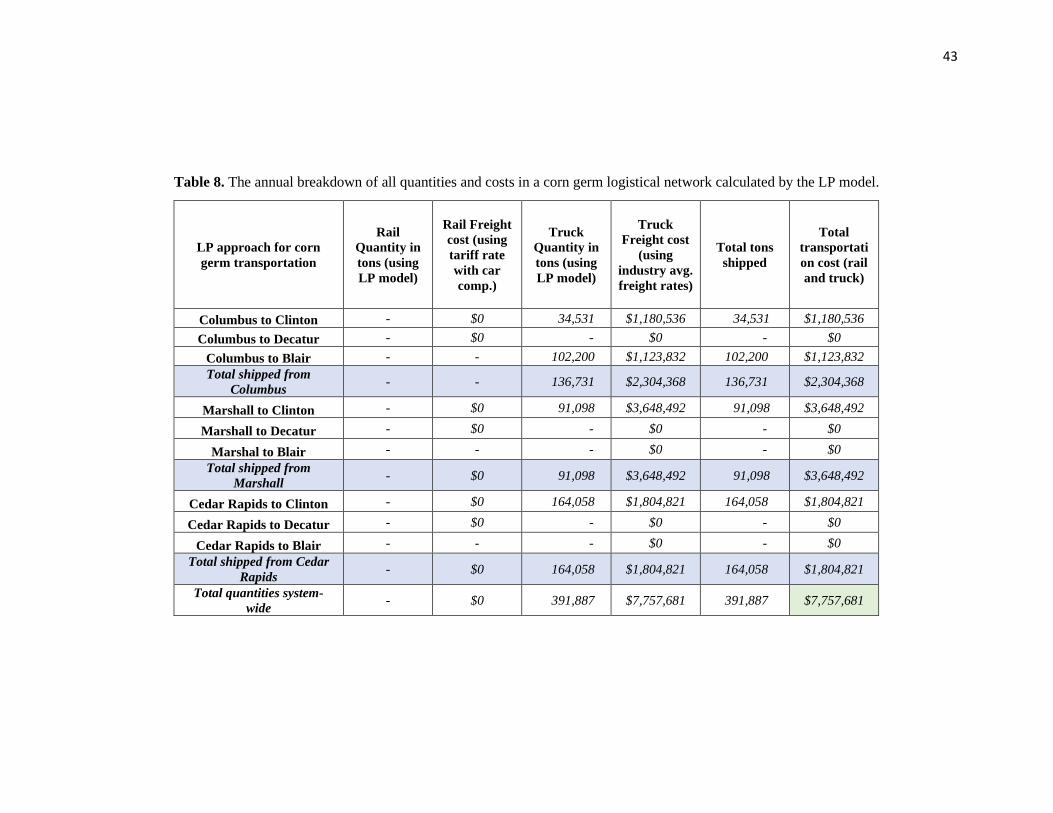
43

Table 8. The annual breakdown of all quantities and costs in a corn germ logistical network calculated by the LP model.

LP approach for corn

germ transportation

Rail

Quantity in

tons (using

LP model)

Rail Freight

cost (using

tariff rate

with car

comp.)

Truck

Quantity in

tons (using

LP model)

Truck

Freight cost

(using

industry avg.

freight rates)

Total tons

shipped

Total

transportati

on cost (rail

and truck)

Columbus to Clinton - $0 34,531 $1,180,536 34,531 $1,180,536

Columbus to Decatur - $0 - $0 - $0

Columbus to Blair - - 102,200 $1,123,832 102,200 $1,123,832

Total shipped from

Columbus - - 136,731 $2,304,368 136,731 $2,304,368

Marshall to Clinton - $0 91,098 $3,648,492 91,098 $3,648,492

Marshall to Decatur - $0 - $0 - $0

Marshal to Blair - - - $0 - $0

Total shipped from

Marshall - $0 91,098 $3,648,492 91,098 $3,648,492

Cedar Rapids to Clinton - $0 164,058 $1,804,821 164,058 $1,804,821

Cedar Rapids to Decatur - $0 - $0 - $0

Cedar Rapids to Blair - - - $0 - $0

Total shipped from Cedar

Rapids - $0 164,058 $1,804,821 164,058 $1,804,821

Total quantities system-

wide - $0 391,887 $7,757,681 391,887 $7,757,681

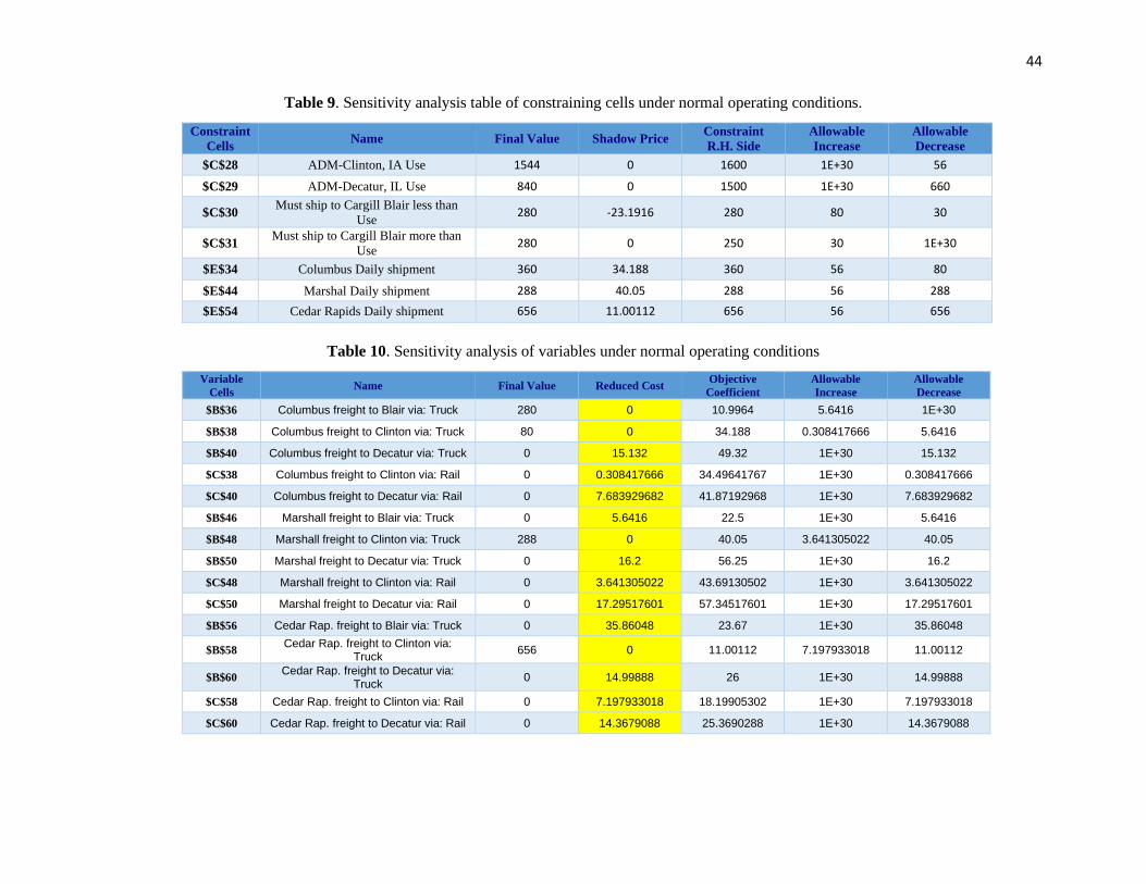
44

Table 9. Sensitivity analysis table of constraining cells under normal operating conditions.

Constraint

Cells Name Final Value Shadow Price

Constraint

R.H. Side

Allowable

Increase

Allowable

Decrease

$C$28 ADM-Clinton, IA Use 1544 0 1600 1E+30 56

$C$29 ADM-Decatur, IL Use 840 0 1500 1E+30 660

$C$30 Must ship to Cargill Blair less than

Use 280 -23.1916 280 80 30

$C$31 Must ship to Cargill Blair more than

Use 280 0 250 30 1E+30

$E$34 Columbus Daily shipment 360 34.188 360 56 80

$E$44 Marshal Daily shipment 288 40.05 288 56 288

$E$54 Cedar Rapids Daily shipment 656 11.00112 656 56 656

Table 10. Sensitivity analysis of variables under normal operating conditions

Variable

Cells Name Final Value Reduced Cost

Objective

Coefficient

Allowable

Increase

Allowable

Decrease

$B$36 Columbus freight to Blair via: Truck 280 0 10.9964 5.6416 1E+30

$B$38 Columbus freight to Clinton via: Truck 80 0 34.188 0.308417666 5.6416

$B$40 Columbus freight to Decatur via: Truck 0 15.132 49.32 1E+30 15.132

$C$38 Columbus freight to Clinton via: Rail 0 0.308417666 34.49641767 1E+30 0.308417666

$C$40 Columbus freight to Decatur via: Rail 0 7.683929682 41.87192968 1E+30 7.683929682

$B$46 Marshall freight to Blair via: Truck 0 5.6416 22.5 1E+30 5.6416

$B$48 Marshall freight to Clinton via: Truck 288 0 40.05 3.641305022 40.05

$B$50 Marshal freight to Decatur via: Truck 0 16.2 56.25 1E+30 16.2

$C$48 Marshall freight to Clinton via: Rail 0 3.641305022 43.69130502 1E+30 3.641305022

$C$50 Marshal freight to Decatur via: Rail 0 17.29517601 57.34517601 1E+30 17.29517601

$B$56 Cedar Rap. freight to Blair via: Truck 0 35.86048 23.67 1E+30 35.86048

$B$58 Cedar Rap. freight to Clinton via:

Truck 656 0 11.00112 7.197933018 11.00112

$B$60 Cedar Rap. freight to Decatur via:

Truck 0 14.99888 26 1E+30 14.99888

$C$58 Cedar Rap. freight to Clinton via: Rail 0 7.197933018 18.19905302 1E+30 7.197933018

$C$60 Cedar Rap. freight to Decatur via: Rail 0 14.3679088 25.3690288 1E+30 14.3679088

45

Table 9.1. Sensitivity analysis table of constraining cells with logistical disruptions.

Constraint

Cells Name Final Value Shadow Price

Constraint

R.H. Side

Allowable

Increase

Allowable

Decrease

$C$28 ADM-Clinton, IA Use 900 -14.3679088 900 284 16

$C$29 ADM-Decatur, IL Use 1484 0 1500 1E+30 16

$C$30 Must ship to Cargill Blair less than Use 280 -31.9179088 280 8 16

$C$31 Must ship to Cargill Blair more than Use 280 0 250 30 1E+30

$E$34 Columbus Daily shipment 360 41.87192968 360 16 360

$E$44 Marshal Daily shipment 288 54.4179088 288 16 8

$E$54 Cedar Rapids Daily shipment 656 25.3690288 656 16 284

Table 10.1. Sensitivity analysis table of variables with logistical disruptions recalculated with new constraints.

Variable

Cells Name Final Value Reduced Cost

Objective

Coefficient

Allowable

Increase

Allowable

Decrease

$B$36 Columbus freight to Blair via: Truck 0 1.042379116 10.9964 1E+30 1.042379116

$B$38 Columbus freight to Clinton via: Truck 0 6.683979116 34.188 1E+30 6.683979116

$C$38 Columbus freight to Clinton via: Rail 0 6.992396782 34.49641767 1E+30 6.992396782

$B$40 Columbus freight to Decatur via: Truck 0 7.448070318 49.32 1E+30 7.448070318

$C$40 Columbus freight to Decatur via: Rail 360 0 41.87192968 1.042379116 41.87192968

$B$46 Marshall freight to Blair via: Truck 280 0 22.5 1.042379116 1E+30

$B$48 Marshall freight to Clinton via: Truck 8 0 40.05 1.832091202 1.042379116

$B$50 Marshal freight to Decatur via: Truck 0 1.832091202 56.25 1E+30 1.832091202

$B$56 Cedar Rap. freight to Blair via: Truck 0 30.21888 23.67 1E+30 30.21888

$B$58 Cedar Rap. freight to Clinton via: Truck 372 0 11.00112 1.042379116 1.832091202

$C$58 Cedar Rap. freight to Clinton via: Rail 0 7.197933018 18.19905302 1E+30 7.197933018

$B$60 Cedar Rap. freight to Decatur via: Truck 0 0.630971202 26 1E+30 0.630971202

$C$60 Cedar Rap. freight to Decatur via: Rail 284 0 25.3690288 0.630971202 1.042379116

46

Table 9.2. Sensitivity analysis table of constraining cells representing Cargill-Blair downtime .

Constraint

Cells Name Final Value Shadow Price

Constraint

R.H. Side

Allowable

Increase

Allowable

Decrease

$C$28 ADM-Clinton, IA Use 1600 -7.375512017 1600 224 136

$C$29 ADM-Decatur, IL Use 1064 0 1500 1E+30 436

$C$30 Must ship to Cargill Blair less than Use 0 -30.87552968 0 224 0

$C$31 Must ship to Cargill Blair more than Use 0 0 0 0 1E+30

$E$34 Columbus Daily shipment 360 41.87192968 360 436 224

$E$44 Marshal Daily shipment 288 51.06681704 288 136 224

$E$54 Cedar Rapids Daily shipment 656 18.37663202 656 136 224

Table 10.2. Sensitivity analysis table of variables recalculated for logistical disruptions with new constraints and increased truck

freight rates.

Variable

Cells Name Final Value Reduced Cost

Objective

Coefficient

Allowable

Increase

Allowable

Decrease

$B$36 Columbus freight to Blair via: Truck 0 0 10.9964 2.308712644 1E+30

$B$38 Columbus freight to Clinton via: Truck 0 6.203582334 40.7 1E+30 6.203582334

$C$38 Columbus freight to Clinton via: Rail 136 0 34.49641767 6.203582334 2.308712644

$B$40 Columbus freight to Decatur via: Truck 0 12.92807032 54.8 1E+30 12.92807032

$C$40 Columbus freight to Decatur via: Rail 224 0 41.87192968 6.278358972 7.375512017

$B$46 Marshall freight to Blair via: Truck 0 2.308712644 22.5 1E+30 2.308712644

$B$48 Marshall freight to Clinton via: Truck 0 0.808694978 44.5 1E+30 0.808694978

$C$48 Marshall freight to Clinton via: Rail 288 0 43.69130502 0.808694978 51.06681704

$B$50 Marshal freight to Decatur via: Truck 0 11.43318296 62.5 1E+30 11.43318296

$C$50 Marshal freight to Decatur via: Rail 0 6.278358972 57.34517601 1E+30 6.278358972

$B$56 Cedar Rap. freight to Blair via: Truck 0 38.79889767 26.3 1E+30 38.79889767

$B$58 Cedar Rap. freight to Clinton via: Truck 656 0 11.00112 6.992396782 18.37663202

$C$58 Cedar Rap. freight to Clinton via: Rail 0 7.197933018 18.19905302 1E+30 7.197933018

$B$60 Cedar Rap. freight to Decatur via: Truck 0 7.623367983 26 1E+30 7.623367983

$C$60 Cedar Rap. freight to Decatur via: Rail 0 6.992396782 25.3690288 1E+30 6.992396782

47

TABLE 11. Linear model case study results showing an optimal daily combination of tons required

to be shipped throughout the network in cells highlighted in yellow.

Total production Daily shipment

Truck Rail 360 360

Cost per ton $11.00

Columbus freight to Blair via: 280 14

Cost per ton $34.19 $34.50

Columbus freight to Clinton via: 80 0

Cost per ton $49.32 $41.87 0

Columbus freight to Decatur via: 0 0

Total Columbus freight cost $5,814.03

Total production Daily shipment

Truck Rail 288 288

Cost per ton $22.50

Marshall freight to Blair via: 0 12

Cost per ton $40.05 $43.69

Marshall freight to Clinton via: 288 0

Cost per ton $56.25 $57.35 0

Marshal freight to Decatur via: 0 0

Total Marshall freight cost $11,534.40

Total production Daily shipment

Truck Rail 656 656

Cost per ton $23.67

Cedar Rap. freight to Blair via: 0 26

Cost per ton $11.00 $18.20

Cedar Rap. freight to Clinton via: 656 0

Cost per ton $26.00 $25.37 0

Cedar Rap. freight to Decatur via: 0 0

Total Cedar Rapids freight cost $7,216.73

Total daily transportation cost $24,565.17

Number of truck

loads shipped (avg.

weight 25 ton load)

Number of ra i l cars

shipped (Avg. car

weight 102 ton)

Cedar Rapids

Columbus

Marshall

Number of truck

loads shipped (avg.

weight 25 ton load)

Number of ra i l cars

shipped (Avg. car

weight 84 ton)

Number of truck

loads shipped (avg.

weight 25 ton load)

Number of ra i l cars

shipped (Avg. car

weight 96 ton)

48

TABLE 12. Linear model case study results showing an optimal daily combination of tons required

to be shipped throughout the network during a winter rail service disruption at ADM-Marshall and

reduced processing capacity at ADM-Clinton.

Total production Daily shipment

Truck Rail 360 360

Cost per ton $11.00

Columbus freight to Blair via: 0 0

Cost per ton $34.19 $34.50

Columbus freight to Clinton via: 0 0

Cost per ton $49.32 $41.87 4

Columbus freight to Decatur via: 0 360

Total Columbus freight cost $15,073.89

Total production Daily shipment

Truck Rail 288 288

Cost per ton $22.50

Marshall freight to Blair via: 280 12

Cost per ton $40.05 $43.69

Marshall freight to Clinton via: 8 NA

Cost per ton $56.25 $57.35 0.0

Marshal freight to Decatur via: 0 NA

Total Marshall freight cost $6,620.40

Total production Daily shipment

Truck Rail 656 656

Cost per ton $23.67

Cedar Rap. freight to Blair via: 0 15

Cost per ton $11.00 $18.20

Cedar Rap. freight to Clinton via: 372 0

Cost per ton $26.00 $25.37 2.8

Cedar Rap. freight to Decatur via: 0 284

Total Cedar Rapids freight cost $11,297.22

Total daily transportation cost $32,991.52

Cedar Rapids

Columbus

Marshall

Number of truck

loads shipped (avg.

weight 25 ton load)

Number of ra i l cars

shipped (Avg. car

weight 84 ton)

Number of truck

loads shipped (avg.

weight 25 ton load)

Number of ra i l cars

shipped (Avg. car

weight 96 ton)

Number of truck

loads shipped (avg.

weight 25 ton load)

Number of ra i l cars

shipped (Avg. car

weight 102 ton)

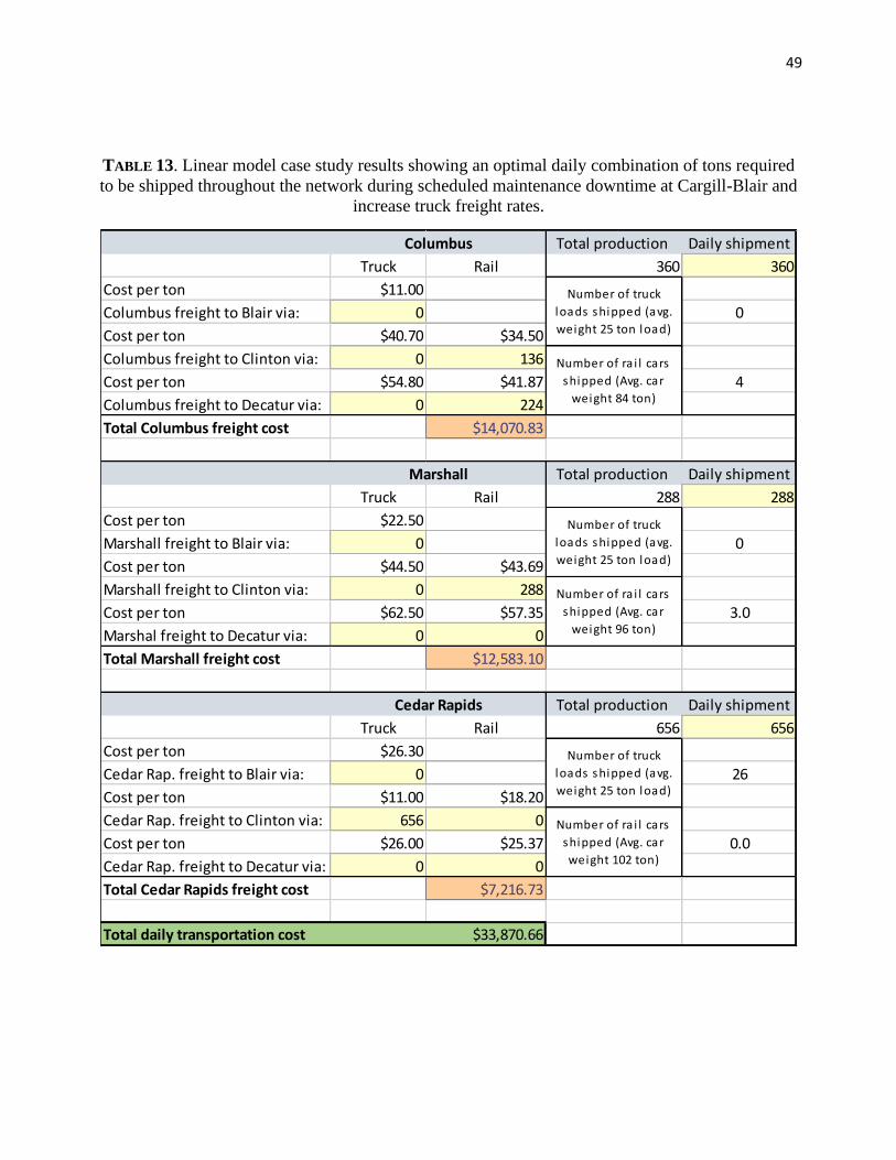
49

TABLE 13. Linear model case study results showing an optimal daily combination of tons required

to be shipped throughout the network during scheduled maintenance downtime at Cargill-Blair and

increase truck freight rates.

Total production Daily shipment

Truck Rail 360 360

Cost per ton $11.00

Columbus freight to Blair via: 0 0

Cost per ton $40.70 $34.50

Columbus freight to Clinton via: 0 136

Cost per ton $54.80 $41.87 4

Columbus freight to Decatur via: 0 224

Total Columbus freight cost $14,070.83

Total production Daily shipment

Truck Rail 288 288

Cost per ton $22.50

Marshall freight to Blair via: 0 0

Cost per ton $44.50 $43.69

Marshall freight to Clinton via: 0 288

Cost per ton $62.50 $57.35 3.0

Marshal freight to Decatur via: 0 0

Total Marshall freight cost $12,583.10

Total production Daily shipment

Truck Rail 656 656

Cost per ton $26.30

Cedar Rap. freight to Blair via: 0 26

Cost per ton $11.00 $18.20

Cedar Rap. freight to Clinton via: 656 0

Cost per ton $26.00 $25.37 0.0

Cedar Rap. freight to Decatur via: 0 0

Total Cedar Rapids freight cost $7,216.73

Total daily transportation cost $33,870.66

Cedar Rapids

Columbus

Marshall

Number of truck

loads shipped (avg.

weight 25 ton load)

Number of ra i l cars

shipped (Avg. car

weight 84 ton)

Number of truck

loads shipped (avg.

weight 25 ton load)

Number of ra i l cars

shipped (Avg. car

weight 96 ton)

Number of truck

loads shipped (avg.

weight 25 ton load)

Number of ra i l cars

shipped (Avg. car

weight 102 ton)

50

Appendix I

Table of all rail shipments between each origin and destination with averages of all the shipments at the top

of each table

Avg. Cubic

Capacity (ft)

Average

pounds per

car

Avg. Cubic

Capacity (ft)

Average

pounds per

car

Avg. Cubic

Capacity (ft)

Average

pounds per

car

6,326 171,180 6,316 167,031 6,340 191,910

Lbs per cu.ft.

of capacity

Average tons

per car

Lbs per cu.ft.

of capacity

Average tons

per car

Lbs per cu.ft.

of capacity

Average tons

per car

27.061 85.59 26.444 83.52 30.270 95.96

Count Ship Date Net Weight Capacity Ship Date Net Weight Capacity Ship Date Net Weight Capacity

1 6/25/2019 171,650 6,240 12/31/2019 172,780 6,350 12/31/2019 192,150 6,350

2 6/25/2019 148,800 6,350 12/31/2019 168,900 6,350 12/31/2019 190,300 6,350

3 6/25/2019 170,900 6,350 12/31/2019 165,700 6,350 12/30/2019 191,900 6,350

4 6/25/2019 169,950 6,350 12/30/2019 177,520 6,350 12/30/2019 191,900 6,350

5 6/24/2019 166,800 6,350 12/30/2019 179,930 6,350 12/30/2019 188,900 6,350

6 6/24/2019 175,000 6,350 12/30/2019 178,660 6,350 12/29/2019 191,100 6,350

7 6/24/2019 159,250 6,350 12/29/2019 177,000 6,240 12/29/2019 190,850 6,350

8 6/24/2019 170,150 6,350 12/29/2019 181,550 6,350 12/29/2019 194,950 6,350

9 6/21/2019 167,800 6,350 12/28/2019 170,750 6,350 12/28/2019 190,450 6,350

10 6/21/2019 171,500 6,350 12/28/2019 179,350 6,350 12/28/2019 192,450 6,350

11 6/19/2019 174,100 6,350 12/28/2019 184,700 6,350 12/26/2019 193,950 6,350

12 6/19/2019 174,100 6,350 12/27/2019 174,700 6,350 12/16/2019 193,800 6,350

13 6/19/2019 170,700 6,350 12/27/2019 180,900 6,350 12/16/2019 188,750 6,350

14 6/18/2019 173,700 6,240 12/27/2019 167,550 6,350 12/15/2019 192,900 6,240

15 6/18/2019 172,550 6,350 12/26/2019 172,720 6,350 12/15/2019 191,500 6,350

16 6/14/2019 156,350 6,240 12/26/2019 167,580 6,350 12/15/2019 190,450 6,350

17 6/14/2019 169,000 6,240 12/26/2019 166,990 6,350 12/14/2019 191,800 6,350

18 6/14/2019 167,550 6,350 12/26/2019 168,450 6,350 12/14/2019 189,600 6,350

19 6/14/2019 170,300 6,350 12/26/2019 162,970 6,350 12/13/2019 190,700 6,350

20 6/13/2019 158,950 6,350 12/26/2019 172,000 6,350 12/13/2019 189,700 6,350

21 6/13/2019 179,500 6,350 12/24/2019 165,980 6,350 12/11/2019 191,350 6,240

22 6/12/2019 172,650 6,350 12/24/2019 168,620 6,350 12/11/2019 190,800 6,350

23 6/12/2019 177,900 6,350 12/24/2019 174,620 6,350 12/11/2019 189,950 6,350

24 6/12/2019 176,650 6,350 12/24/2019 158,400 6,350 12/11/2019 191,000 6,350

25 5/20/2019 174,620 6,240 12/23/2019 175,100 6,240 12/10/2019 191,400 6,350

26 5/20/2019 166,750 6,350 12/23/2019 170,350 6,350 12/9/2019 190,100 6,350

27 5/20/2019 173,900 6,350 12/23/2019 178,350 6,350 12/9/2019 191,450 6,350

28 5/20/2019 165,540 6,350 12/23/2019 170,950 6,350 12/8/2019 192,500 6,350

29 5/19/2019 161,150 6,350 12/22/2019 177,700 6,350 12/8/2019 193,100 6,350

30 5/19/2019 166,600 6,350 12/21/2019 167,200 6,350 12/7/2019 193,800 6,350

31 5/19/2019 173,300 6,350 12/21/2019 172,100 6,350 12/6/2019 188,050 6,350

32 5/18/2019 171,550 6,350 12/21/2019 176,000 6,350 12/6/2019 192,950 6,350

33 5/18/2019 169,950 6,350 12/21/2019 181,700 6,350 12/5/2019 190,150 6,350

34 5/17/2019 173,700 6,240 12/21/2019 171,850 6,350 12/4/2019 189,650 6,350

35 5/17/2019 175,050 6,350 12/21/2019 179,050 6,350 12/2/2019 192,650 6,240

36 5/17/2019 168,020 6,350 12/21/2019 174,450 6,350 12/2/2019 190,950 6,350

37 5/16/2019 177,500 6,350 12/18/2019 155,000 6,350 12/2/2019 191,550 6,350

38 5/16/2019 174,000 6,350 12/18/2019 168,050 6,350 12/1/2019 191,750 6,350

39 5/15/2019 172,300 6,350 12/18/2019 161,420 6,350 12/1/2019 191,800 6,350

40 5/15/2019 165,250 6,350 12/18/2019 166,400 6,350 11/30/2019 193,050 6,350

41 5/15/2019 176,600 6,350 12/18/2019 166,350 6,350 11/30/2019 189,700 6,350

42 5/14/2019 162,450 6,350 12/17/2019 158,450 6,350 11/30/2019 191,200 6,350

43 5/14/2019 167,400 6,350 12/17/2019 160,300 6,350 11/30/2019 191,700 6,350

44 5/13/2019 171,850 6,240 12/17/2019 164,200 6,350 11/30/2019 194,200 6,350

45 5/13/2019 166,650 6,350 12/17/2019 156,720 6,350 11/30/2019 190,450 6,350

46 5/13/2019 169,750 6,350 12/17/2019 162,150 6,350 11/30/2019 190,900 6,350

47 5/13/2019 171,500 6,350 12/17/2019 172,300 6,350 11/27/2019 191,150 6,240

48 5/13/2019 160,600 6,350 12/17/2019 172,550 6,350 11/27/2019 190,850 6,350

49 5/13/2019 167,450 6,350 12/17/2019 175,670 6,350 11/27/2019 190,250 6,350

50 5/13/2019 170,950 6,350 12/15/2019 171,650 6,350 11/27/2019 182,300 6,350

51 5/13/2019 165,550 6,200 12/15/2019 163,300 6,350 11/27/2019 190,850 6,350

52 5/13/2019 168,400 6,350 12/14/2019 160,950 6,240 11/27/2019 188,550 6,350

53 5/13/2019 158,950 6,350 12/14/2019 176,900 6,350 11/24/2019 193,250 6,240

54 5/13/2019 179,680 6,350 12/14/2019 175,500 6,350 11/18/2019 190,950 6,350

55 5/10/2019 173,450 6,350 12/14/2019 161,100 6,350 11/18/2019 192,150 6,350

56 5/10/2019 168,400 6,350 12/13/2019 163,540 6,350 11/18/2019 192,850 6,350

57 5/10/2019 178,650 6,350 12/13/2019 165,450 6,350 11/18/2019 190,700 6,350

58 5/10/2019 172,250 6,350 12/13/2019 144,480 6,350 11/18/2019 192,200 6,350

59 5/9/2019 168,200 6,350 12/13/2019 156,850 6,350 11/18/2019 192,150 6,350

60 5/9/2019 170,600 6,350 12/13/2019 153,900 6,350 11/18/2019 190,150 6,350

Columbus to Clinton Columbus to Decatur Marshall to Clinton

51

61 5/9/2019 177,050 6,350 12/12/2019 162,350 6,350 11/18/2019 193,550 6,350

62 5/9/2019 173,250 6,350 12/12/2019 159,650 6,350 11/18/2019 191,050 6,350

63 5/8/2019 164,250 6,240 12/12/2019 158,250 6,350 11/18/2019 190,950 6,350

64 5/8/2019 161,050 6,350 12/12/2019 158,200 6,350 11/18/2019 192,500 6,350

65 5/8/2019 165,300 6,350 12/11/2019 169,000 6,350 11/18/2019 192,800 6,350

66 5/8/2019 156,400 6,350 12/10/2019 164,350 6,350 11/18/2019 191,350 6,350

67 5/8/2019 161,850 6,350 12/10/2019 166,800 6,350 11/18/2019 191,600 6,350

68 5/6/2019 165,850 6,350 12/10/2019 165,700 6,350 11/18/2019 190,550 6,350

69 5/6/2019 164,350 6,200 12/9/2019 171,330 6,350 11/18/2019 191,750 6,350

70 5/6/2019 159,600 6,350 12/9/2019 167,200 6,350 11/18/2019 191,450 6,350

71 4/10/2019 162,700 6,350 12/9/2019 169,900 6,350 11/18/2019 192,000 6,350

72 4/10/2019 162,690 6,350 12/8/2019 155,500 6,350 11/18/2019 191,450 6,350

73 4/10/2019 174,700 6,350 12/8/2019 156,750 6,350 11/11/2019 191,000 6,350

74 4/9/2019 174,800 6,350 12/8/2019 146,000 6,350 11/11/2019 189,900 6,350

75 4/9/2019 159,300 6,350 12/8/2019 161,570 6,350 11/11/2019 188,500 6,350

76 4/9/2019 160,200 6,350 12/7/2019 169,900 6,240 11/11/2019 193,500 6,350

77 4/9/2019 173,850 6,350 12/7/2019 158,400 6,350 11/11/2019 190,500 6,350

78 4/9/2019 167,750 6,350 12/7/2019 161,600 6,350 11/11/2019 191,200 6,350

79 4/8/2019 166,200 6,350 12/7/2019 138,200 5,460 11/9/2019 192,050 6,350

80 4/8/2019 170,150 6,350 12/7/2019 164,000 6,350 11/9/2019 191,600 6,350

81 4/8/2019 170,060 6,350 12/6/2019 166,050 6,350 11/9/2019 194,800 6,350

82 4/8/2019 173,000 6,350 12/6/2019 165,450 6,350 11/9/2019 191,650 6,350

83 4/8/2019 166,500 6,350 12/6/2019 162,700 6,350 11/9/2019 191,750 6,350

84 4/8/2019 161,000 6,350 12/5/2019 166,000 6,350 11/9/2019 195,400 6,350

85 4/7/2019 139,000 5,160 12/5/2019 181,110 6,350 11/9/2019 189,900 6,350

86 4/7/2019 173,500 6,350 12/5/2019 174,900 6,350 11/9/2019 191,000 6,350

87 4/7/2019 167,950 6,350 12/4/2019 177,300 6,350 11/9/2019 188,950 6,350

88 4/7/2019 165,750 6,350 12/4/2019 162,100 6,350 11/9/2019 189,400 6,350

89 4/7/2019 173,400 6,350 12/2/2019 153,700 6,350 11/9/2019 189,050 6,350

90 4/6/2019 179,900 6,350 12/2/2019 174,500 6,350 11/5/2019 190,600 6,350

91 4/6/2019 188,550 6,350 12/2/2019 164,010 6,350 11/5/2019 191,100 6,350

92 4/5/2019 179,050 6,350 12/2/2019 164,050 6,350 11/5/2019 189,450 6,350

93 4/5/2019 176,150 6,350 12/2/2019 161,050 6,350 11/4/2019 191,500 6,350

94 4/4/2019 194,340 6,240 12/2/2019 158,450 6,350 11/4/2019 191,950 6,350

95 4/4/2019 167,750 6,350 12/2/2019 139,400 5,460 11/4/2019 192,900 6,350

96 4/4/2019 163,700 6,350 12/2/2019 155,350 6,350 11/4/2019 189,900 6,350

97 4/3/2019 193,700 6,350 12/2/2019 160,700 6,350 11/3/2019 191,850 6,350

98 4/3/2019 172,690 6,350 12/2/2019 161,650 6,350 11/3/2019 193,150 6,350

99 4/1/2019 176,430 6,240 12/2/2019 156,650 6,350 11/3/2019 192,500 6,350

100 4/1/2019 179,950 6,350 12/2/2019 166,800 6,350 11/2/2019 195,450 6,240

101 4/1/2019 182,950 6,350 11/27/2019 166,680 6,350 11/2/2019 191,150 6,350

102 4/1/2019 177,750 6,350 11/27/2019 162,100 6,350 11/1/2019 194,950 6,240

103 4/1/2019 174,650 6,350 11/27/2019 163,410 6,350 11/1/2019 192,900 6,350

104 4/1/2019 171,000 6,350 11/27/2019 141,350 5,250 11/1/2019 191,200 6,350

105 3/28/2019 208,900 6,350 11/27/2019 162,750 6,350 11/1/2019 192,000 6,350

106 3/28/2019 217,650 6,350 11/27/2019 137,950 5,150 10/31/2019 190,500 6,350

107 3/28/2019 215,400 6,350 11/27/2019 155,200 6,350 10/31/2019 189,200 6,350

108 11/27/2019 158,350 6,350 10/31/2019 191,350 6,350

109 11/27/2019 161,050 6,350 10/30/2019 192,300 6,240

110 11/27/2019 168,680 6,350 10/30/2019 191,700 6,350

111 11/24/2019 163,700 6,350 10/30/2019 191,650 6,350

112 11/24/2019 162,250 6,350 10/29/2019 192,250 6,350

113 11/24/2019 165,650 6,350 10/29/2019 192,300 6,350

114 11/23/2019 164,850 6,350 10/29/2019 193,250 6,350

115 11/23/2019 161,970 6,350 10/28/2019 193,900 6,350

116 11/22/2019 157,700 6,350 10/28/2019 193,050 6,350

117 11/22/2019 164,550 6,350 10/28/2019 192,200 6,350

118 11/22/2019 170,550 6,350 10/28/2019 192,550 6,350

119 11/21/2019 165,150 6,350 10/27/2019 192,350 6,240

120 11/21/2019 169,810 6,350 10/27/2019 191,250 6,350

121 11/21/2019 163,450 6,350 10/27/2019 193,050 6,350

122 11/21/2019 166,500 6,350 10/26/2019 193,950 6,350

123 11/21/2019 167,500 6,350 10/25/2019 193,900 6,350

124 11/21/2019 153,500 6,350 10/25/2019 191,350 6,350

125 11/21/2019 169,650 6,350 10/25/2019 191,450 6,350

126 11/21/2019 171,850 6,350 10/25/2019 189,650 6,350

127 11/21/2019 166,750 6,350 10/24/2019 190,100 6,350

128 11/18/2019 167,550 6,350 10/24/2019 192,050 6,350

129 11/18/2019 167,550 6,350 10/23/2019 193,100 6,350

130 11/18/2019 176,300 6,350 10/23/2019 193,150 6,350

52

131 11/18/2019 170,860 6,350 10/23/2019 191,850 6,350

132 11/18/2019 170,800 6,350 10/22/2019 193,900 6,240

133 11/18/2019 157,200 6,350 10/22/2019 191,650 6,350

134 11/18/2019 173,020 6,350 10/22/2019 192,050 6,350

135 11/18/2019 171,700 6,350 10/21/2019 192,400 6,350

136 11/18/2019 161,120 6,350 10/21/2019 191,550 6,350

137 11/18/2019 173,150 6,350 10/21/2019 192,300 6,350

138 11/18/2019 166,300 6,350 10/20/2019 191,400 6,350

139 11/18/2019 175,500 6,350 10/20/2019 193,800 6,350

140 11/15/2019 167,200 6,240 10/20/2019 192,500 6,350

141 11/15/2019 164,650 6,240 10/20/2019 191,700 6,350

142 11/15/2019 170,700 6,350 10/18/2019 190,200 6,350

143 11/15/2019 161,550 6,350 10/18/2019 193,250 6,350

144 11/15/2019 152,700 6,350 10/18/2019 190,250 6,350

145 11/15/2019 158,150 6,350 10/17/2019 192,350 6,350

146 11/15/2019 156,010 6,350 10/17/2019 193,850 6,350

147 11/15/2019 166,450 6,350 10/17/2019 193,550 6,350

148 11/15/2019 164,350 6,350 10/16/2019 192,200 6,240

149 11/15/2019 158,550 6,350 10/16/2019 191,250 6,350

150 11/15/2019 173,050 6,350 10/16/2019 191,400 6,350

151 11/15/2019 161,450 6,350 10/16/2019 191,100 6,350

152 11/11/2019 167,650 6,350 10/15/2019 191,850 6,350

153 11/11/2019 150,750 6,350 10/15/2019 191,450 6,350

154 11/11/2019 152,500 6,350 10/15/2019 190,650 6,350

155 11/11/2019 160,650 6,350 10/14/2019 191,050 6,350

156 11/11/2019 163,050 6,350 10/14/2019 195,000 6,350

157 11/11/2019 160,100 6,350 10/14/2019 191,600 6,350

158 11/11/2019 163,290 6,350 10/13/2019 193,200 6,350

159 11/11/2019 160,800 6,350 10/13/2019 191,500 6,350

160 11/11/2019 153,500 6,350 10/13/2019 191,300 6,350

161 11/11/2019 165,500 6,350 10/12/2019 191,100 6,350

162 11/11/2019 158,800 6,350 10/12/2019 191,400 6,350

163 11/11/2019 155,850 6,350 10/11/2019 193,450 6,240

164 11/5/2019 151,200 5,150 10/11/2019 192,400 6,240

165 11/4/2019 167,300 6,350 10/11/2019 193,050 6,350

166 11/4/2019 181,200 6,350 10/10/2019 190,500 6,350

167 11/4/2019 165,300 6,350 10/10/2019 194,700 6,350

168 11/4/2019 171,200 6,350 10/10/2019 191,550 6,350

169 11/3/2019 167,750 6,350 10/9/2019 190,900 6,350

170 11/3/2019 165,100 6,350 10/9/2019 189,750 6,350

171 11/3/2019 160,100 6,350 10/9/2019 192,900 6,350

172 11/3/2019 165,200 6,350 10/8/2019 192,950 6,350

173 11/2/2019 168,900 6,350 10/8/2019 193,350 6,350

174 11/2/2019 167,250 6,350 10/7/2019 192,500 6,350

175 11/2/2019 173,360 6,350 10/7/2019 189,200 6,350

176 11/1/2019 165,550 6,240 10/7/2019 190,300 6,350

177 11/1/2019 147,900 6,240 10/7/2019 191,750 6,350

178 11/1/2019 162,650 6,350 10/6/2019 194,150 6,350

179 11/1/2019 161,250 6,350 10/6/2019 191,450 6,350

180 11/1/2019 169,250 6,350 10/6/2019 191,600 6,350

181 10/31/2019 152,300 6,350 10/5/2019 192,950 6,240

182 10/31/2019 148,000 6,350 10/5/2019 190,950 6,350

183 10/31/2019 176,150 6,350 10/4/2019 193,900 6,350

184 10/30/2019 159,000 6,240 10/4/2019 193,610 6,350

185 10/30/2019 154,750 6,350 10/4/2019 193,600 6,350

186 10/30/2019 131,150 5,400 10/3/2019 192,630 6,350

187 10/30/2019 168,350 6,350 10/3/2019 192,300 6,350

188 10/30/2019 154,900 6,350 10/3/2019 192,100 6,350

189 10/29/2019 166,400 6,240 10/2/2019 194,620 6,240

190 10/29/2019 158,200 6,350 10/2/2019 189,350 6,350

191 10/29/2019 157,200 6,350 10/2/2019 191,600 6,350

192 10/29/2019 158,130 6,350 10/2/2019 192,100 6,350

193 10/29/2019 152,740 6,350 10/1/2019 192,750 6,350

194 10/29/2019 153,250 6,350 10/1/2019 191,550 6,350

195 10/28/2019 148,500 6,350 9/30/2019 191,200 6,350

196 10/28/2019 156,950 6,350 9/30/2019 190,530 6,350

197 10/28/2019 167,950 6,350 9/30/2019 192,230 6,350

198 10/28/2019 154,520 6,350 9/30/2019 191,850 6,350

199 10/28/2019 167,610 6,350 9/30/2019 191,200 6,350

200 10/28/2019 159,600 6,350 9/30/2019 192,900 6,350

53

201 10/28/2019 170,600 6,350 9/30/2019 190,390 6,350

202 10/28/2019 160,650 6,350 9/27/2019 193,090 6,240

203 10/27/2019 157,350 6,350 9/27/2019 194,200 6,350

204 10/27/2019 163,260 6,350 9/26/2019 192,300 6,350

205 10/26/2019 160,300 6,350 9/26/2019 191,300 6,350

206 10/25/2019 163,100 6,350 9/26/2019 193,350 6,350

207 10/25/2019 171,100 6,350 9/26/2019 192,800 6,350

208 10/25/2019 152,800 6,350 9/25/2019 190,250 6,350

209 10/25/2019 161,500 6,350 9/24/2019 191,530 6,240

210 10/24/2019 169,300 6,350 9/24/2019 191,130 6,350

211 10/24/2019 180,850 6,350 9/24/2019 192,050 6,350

212 10/24/2019 164,000 6,350 9/23/2019 192,350 6,350

213 10/24/2019 159,650 6,350 9/23/2019 192,000 6,350

214 10/23/2019 168,950 6,350 9/23/2019 193,800 6,350

215 10/23/2019 168,150 6,350 9/23/2019 193,650 6,350

216 10/22/2019 155,800 6,350 9/22/2019 192,850 6,350

217 10/22/2019 164,800 6,350 9/22/2019 193,850 6,350

218 10/22/2019 159,450 6,350 9/22/2019 193,700 6,350

219 10/21/2019 166,410 6,350 9/21/2019 192,900 6,350

220 10/21/2019 157,200 6,350 9/21/2019 195,700 6,350

221 10/21/2019 160,100 6,350 9/21/2019 192,200 6,350

222 10/21/2019 158,550 6,350 9/20/2019 195,200 6,240

223 10/21/2019 160,600 6,350 9/20/2019 190,930 6,350

224 10/20/2019 166,900 6,350 9/19/2019 192,080 6,350

225 10/20/2019 142,400 5,430 9/19/2019 192,150 6,350

226 10/20/2019 171,150 6,350 9/19/2019 193,600 6,350

227 10/20/2019 164,900 6,350 9/19/2019 192,250 6,350

228 10/19/2019 176,140 6,240 9/18/2019 190,600 6,350

229 10/19/2019 174,300 6,350 9/18/2019 194,050 6,350

230 10/19/2019 179,750 6,350 9/18/2019 190,520 6,350

231 10/18/2019 168,550 6,350 9/17/2019 190,460 6,350

232 10/18/2019 159,650 6,350 9/16/2019 191,600 6,350

233 10/18/2019 169,050 6,350 9/16/2019 189,250 6,350

234 10/17/2019 151,200 6,240 9/16/2019 191,150 6,350

235 10/17/2019 159,700 6,350 9/15/2019 188,440 6,350

236 10/17/2019 173,850 6,350 9/15/2019 192,300 6,350

237 10/16/2019 178,300 6,350 9/15/2019 193,100 6,350

238 10/15/2019 186,200 6,350 9/14/2019 192,800 6,240

239 10/14/2019 174,350 6,350 9/14/2019 192,150 6,350

240 10/14/2019 189,550 6,350 9/13/2019 189,550 6,350

241 10/14/2019 179,200 6,350 9/13/2019 193,480 6,350

242 10/13/2019 178,400 6,350 9/13/2019 191,450 6,200

243 10/12/2019 155,750 6,350 9/13/2019 191,430 6,350

244 10/12/2019 172,800 6,350 9/12/2019 193,500 6,350

245 10/12/2019 159,450 6,350 9/12/2019 194,000 6,350

246 10/11/2019 175,100 6,350 9/11/2019 191,890 6,350

247 10/11/2019 179,150 6,350 9/11/2019 190,950 6,350

248 10/10/2019 169,200 6,350 9/11/2019 193,150 6,350

249 10/10/2019 193,550 6,350 9/10/2019 190,900 6,350

250 9/24/2019 155,750 6,350 9/10/2019 192,810 6,350

251 9/23/2019 155,000 6,350 9/10/2019 191,850 6,350

252 9/23/2019 164,550 6,350 9/10/2019 192,450 6,350

253 9/23/2019 161,200 6,350 9/9/2019 193,190 6,350

254 9/23/2019 167,000 6,350 9/9/2019 192,450 6,350

255 9/22/2019 212,150 6,240 9/9/2019 192,740 6,350

256 9/22/2019 160,900 6,350 9/8/2019 191,020 6,350

257 9/22/2019 162,550 6,350 9/8/2019 191,470 6,350

258 9/21/2019 158,410 6,350 9/7/2019 193,100 6,350

259 9/21/2019 169,770 6,350 9/7/2019 194,300 6,350

260 9/21/2019 169,850 6,350 9/7/2019 191,230 6,350

261 9/20/2019 164,400 6,350 9/6/2019 192,950 6,350

262 9/20/2019 163,300 6,350 9/6/2019 191,280 6,350

263 9/20/2019 165,450 6,350 9/5/2019 192,620 6,350

264 9/19/2019 173,950 6,350 9/5/2019 193,250 6,350

265 9/19/2019 163,450 6,350 9/4/2019 193,120 6,350

266 9/18/2019 156,590 5,800 9/4/2019 191,530 6,350

267 9/18/2019 168,500 6,200 9/4/2019 191,120 6,350

268 9/18/2019 164,700 6,350 9/3/2019 193,420 6,350

269 9/18/2019 168,200 6,350 9/3/2019 193,620 6,350

270 9/17/2019 171,850 6,350 9/2/2019 195,210 6,350

54

271 9/17/2019 168,200 6,350 9/2/2019 192,250 6,350

272 9/16/2019 169,650 6,350 9/2/2019 191,500 6,350

273 9/16/2019 166,050 6,350 9/1/2019 193,200 6,350

274 9/16/2019 181,700 6,350 9/1/2019 195,700 6,350

275 9/16/2019 172,950 6,350 9/1/2019 191,170 6,350

276 9/16/2019 162,750 6,350 8/31/2019 192,900 6,350

277 9/16/2019 167,900 6,350 8/31/2019 191,150 6,350

278 9/15/2019 173,600 6,350 8/31/2019 193,200 6,350

279 9/15/2019 160,700 6,350 8/30/2019 192,100 6,350

280 9/15/2019 168,720 6,350 8/30/2019 192,550 6,350

281 9/14/2019 177,750 6,240 8/30/2019 193,050 6,350

282 9/14/2019 170,150 6,350 8/29/2019 190,130 6,350

283 9/14/2019 169,550 6,350 8/29/2019 190,300 6,350

284 9/14/2019 169,650 6,350 8/19/2019 191,200 6,350

285 9/14/2019 183,200 6,350 8/19/2019 193,250 6,350

286 9/12/2019 187,950 6,350 8/19/2019 191,400 6,350

287 9/12/2019 177,150 6,350 8/19/2019 191,410 6,350

288 9/11/2019 167,400 6,350 8/18/2019 191,590 6,350

289 9/11/2019 166,700 6,350 8/18/2019 194,950 6,350

290 9/11/2019 167,100 6,350 8/18/2019 191,150 6,350

291 9/10/2019 159,250 6,350 8/17/2019 188,710 6,350

292 9/10/2019 157,800 6,350 8/17/2019 187,400 6,350

293 9/9/2019 159,700 6,350 8/16/2019 193,850 6,350

294 9/9/2019 162,300 6,350 8/16/2019 191,150 6,350

295 9/9/2019 165,850 6,350 8/15/2019 192,250 6,350

296 9/9/2019 167,550 6,350 8/15/2019 193,260 6,350

297 9/8/2019 169,750 6,350 8/15/2019 191,600 6,350

298 9/8/2019 167,000 6,350 8/14/2019 193,690 6,240

299 9/7/2019 158,900 6,350 8/14/2019 191,860 6,350

300 9/7/2019 168,250 6,350 8/14/2019 191,950 6,350

301 9/7/2019 164,400 6,350 8/14/2019 189,650 6,350

302 9/7/2019 166,950 6,350 8/13/2019 190,740 6,350

303 9/6/2019 159,050 6,350 8/13/2019 191,080 6,350

304 9/6/2019 158,250 6,350 8/13/2019 191,650 6,350

305 9/6/2019 168,100 6,350 8/12/2019 190,200 6,350

306 9/6/2019 165,400 6,350 8/12/2019 191,050 6,350

307 9/5/2019 175,170 6,350 8/12/2019 189,900 6,350

308 9/5/2019 158,750 6,350 8/11/2019 193,650 6,350

309 9/4/2019 158,250 6,350 8/11/2019 192,650 6,350

310 9/4/2019 144,400 6,350 8/11/2019 192,050 6,350

311 9/4/2019 161,450 6,350 8/10/2019 191,950 6,350

312 9/4/2019 162,030 6,350 8/10/2019 190,450 6,350

313 9/4/2019 162,000 6,350 8/10/2019 191,650 6,350

314 9/3/2019 153,050 6,350 8/9/2019 192,200 6,350

315 9/3/2019 148,450 6,350 8/9/2019 192,150 6,350

316 9/3/2019 158,750 6,350 8/9/2019 191,460 6,350

317 9/2/2019 151,050 6,350 8/8/2019 192,400 6,350

318 9/2/2019 171,800 6,350 8/8/2019 193,700 6,350

319 9/2/2019 157,350 6,350 8/8/2019 190,610 6,350

320 9/2/2019 153,750 6,350 8/7/2019 191,870 6,350

321 9/1/2019 162,800 6,240 8/7/2019 192,800 6,350

322 9/1/2019 159,650 6,350 8/7/2019 191,090 6,350

323 9/1/2019 158,350 6,350 8/6/2019 191,900 6,350

324 9/1/2019 163,150 6,350 8/6/2019 189,400 6,350

325 8/31/2019 150,100 6,350 8/6/2019 191,030 6,350

326 8/31/2019 124,050 5,200 8/5/2019 193,500 6,240

327 8/31/2019 171,800 6,350 8/5/2019 193,000 6,350

328 8/31/2019 169,450 6,350 8/5/2019 191,050 6,350

329 8/30/2019 169,400 6,350 8/5/2019 193,320 6,350

330 8/30/2019 164,100 6,350 8/4/2019 191,110 6,350

331 8/30/2019 156,900 6,350 8/4/2019 191,200 6,350

332 8/29/2019 169,000 6,350 8/3/2019 190,750 6,350

333 8/29/2019 156,850 6,350 8/3/2019 193,970 6,350

334 8/29/2019 159,950 6,350 8/3/2019 191,270 6,350

335 8/29/2019 158,200 6,350 8/2/2019 194,300 6,350

336 8/29/2019 159,300 6,350 8/2/2019 194,100 6,350

337 8/28/2019 158,050 6,350 8/1/2019 193,450 6,350

338 8/28/2019 157,550 6,350 8/1/2019 191,840 6,350

339 8/28/2019 166,050 6,350 8/1/2019 194,810 6,350

340 8/27/2019 162,850 6,350 8/1/2019 191,060 6,350

55

341 8/27/2019 164,500 6,350 7/31/2019 193,850 6,350

342 8/27/2019 160,300 6,350 7/31/2019 192,650 6,350

343 8/26/2019 155,000 6,350 7/30/2019 193,770 6,350

344 8/26/2019 155,200 6,350 7/30/2019 193,900 6,350

345 8/26/2019 155,400 6,350 7/30/2019 192,150 6,350

346 8/26/2019 163,200 6,350 7/30/2019 192,350 6,350

347 8/25/2019 174,250 6,240 7/30/2019 189,200 6,350

348 8/25/2019 160,050 6,350 7/29/2019 192,110 6,240

349 8/25/2019 168,900 6,350 7/29/2019 193,540 6,350

350 8/24/2019 156,150 6,240 7/29/2019 193,350 6,350

351 8/24/2019 161,200 6,350 7/28/2019 192,850 6,240

352 8/24/2019 156,200 6,350 7/28/2019 192,250 6,350

353 8/23/2019 167,050 6,350 7/27/2019 191,000 6,350

354 8/23/2019 157,450 6,200 7/27/2019 192,000 6,350

355 8/22/2019 149,500 6,350 7/27/2019 192,400 6,350

356 8/22/2019 155,700 6,350 7/26/2019 191,400 6,350

357 8/22/2019 170,650 6,350 7/26/2019 191,150 6,350

358 8/22/2019 146,500 6,350 7/26/2019 192,030 6,350

359 8/21/2019 152,600 6,350 7/25/2019 192,860 6,350

360 8/21/2019 166,650 6,350 7/25/2019 191,400 6,350

361 8/21/2019 165,900 6,350 7/24/2019 190,750 6,350

362 8/20/2019 164,100 6,350 7/24/2019 193,600 6,350

363 8/20/2019 145,550 6,350 7/24/2019 191,550 6,350

364 8/19/2019 158,050 6,350 7/23/2019 193,200 6,240

365 8/19/2019 164,500 6,350 7/23/2019 191,800 6,350

366 8/19/2019 152,060 6,350 7/23/2019 190,300 6,350

367 8/18/2019 166,550 6,350 7/22/2019 190,410 6,350

368 8/18/2019 169,050 6,350 7/22/2019 191,000 6,350

369 8/18/2019 166,900 6,350 7/22/2019 193,120 6,350

370 8/18/2019 167,250 6,350 7/21/2019 190,620 6,350

371 8/17/2019 155,250 6,350 7/21/2019 193,650 6,350

372 8/17/2019 163,000 6,350 7/21/2019 193,420 6,350

373 8/17/2019 137,580 5,430 7/20/2019 193,050 6,350

374 8/16/2019 154,550 5,800 7/20/2019 192,520 6,350

375 8/15/2019 172,650 6,350 7/20/2019 191,700 6,350

376 8/15/2019 158,250 6,350 7/19/2019 191,200 6,350

377 8/15/2019 168,400 6,350 7/19/2019 191,280 6,350

378 8/13/2019 161,500 6,350 7/19/2019 193,550 6,350

379 8/13/2019 172,650 6,350 7/19/2019 194,950 6,350

380 8/13/2019 162,450 6,350 7/18/2019 193,350 6,350

381 8/12/2019 154,200 6,350 7/18/2019 195,450 6,350

382 8/12/2019 157,700 6,350 7/17/2019 192,000 6,350

383 8/12/2019 162,900 6,350 7/17/2019 192,650 6,350

384 8/12/2019 172,800 6,350 7/17/2019 191,700 6,350

385 8/12/2019 169,650 6,350 7/16/2019 194,600 6,350

386 8/11/2019 159,750 6,350 7/16/2019 192,630 6,350

387 8/11/2019 163,550 6,350 7/16/2019 189,990 6,350

388 8/11/2019 151,600 6,350 7/15/2019 194,550 6,350

389 8/11/2019 169,000 6,350 7/15/2019 190,970 6,350

390 8/11/2019 169,400 6,350 7/15/2019 192,140 6,350

391 8/10/2019 163,750 6,350 7/14/2019 192,380 6,240

392 8/10/2019 163,950 6,350 7/14/2019 193,290 6,350

393 8/10/2019 166,150 6,350 7/14/2019 191,600 6,350

394 8/10/2019 169,500 6,350 7/14/2019 192,220 6,200

395 8/10/2019 155,700 6,350 7/13/2019 190,950 6,350

396 8/10/2019 163,650 6,350 7/13/2019 192,200 6,350

397 8/9/2019 163,000 6,240 7/13/2019 192,280 6,350

398 8/9/2019 170,390 6,350 7/13/2019 191,400 6,350

399 8/9/2019 174,750 6,350 7/12/2019 191,350 6,350

400 8/8/2019 160,800 6,350 7/12/2019 193,350 6,350

401 8/7/2019 155,000 6,350 7/12/2019 192,100 6,350

402 8/7/2019 163,450 6,350 7/11/2019 190,150 6,350

403 8/7/2019 156,300 6,350 7/11/2019 193,600 6,350

404 8/6/2019 169,750 6,350 7/11/2019 188,950 6,350

405 8/6/2019 173,950 6,350 7/10/2019 192,590 6,350

406 8/5/2019 165,220 6,350 7/10/2019 192,300 6,350

407 8/5/2019 179,750 6,350 7/9/2019 194,350 6,240

408 8/5/2019 168,000 6,350 7/9/2019 192,790 6,350

409 8/5/2019 175,800 6,350 7/9/2019 191,200 6,350

410 8/4/2019 169,850 6,350 7/9/2019 193,300 6,350

56

411 8/4/2019 156,400 6,350 7/8/2019 193,750 6,350

412 8/4/2019 169,800 6,350 7/8/2019 190,830 6,350

413 8/3/2019 163,900 6,350 7/8/2019 193,060 6,350

414 8/3/2019 168,450 6,350 7/7/2019 192,050 6,350

415 8/2/2019 164,250 6,240 7/7/2019 191,180 6,350

416 8/2/2019 154,900 6,350 7/7/2019 193,470 6,350

417 8/2/2019 164,800 6,350 7/6/2019 191,810 6,350

418 8/2/2019 165,850 6,350 7/6/2019 195,150 6,350

419 8/1/2019 164,800 6,350 7/6/2019 193,350 6,350

420 8/1/2019 167,300 6,350 7/6/2019 190,850 6,350

421 8/1/2019 159,000 6,200 7/5/2019 192,610 6,240

422 8/1/2019 166,400 6,350 7/5/2019 192,050 6,350

423 8/1/2019 154,000 6,350 7/5/2019 192,420 6,350

424 8/1/2019 155,400 6,350 7/5/2019 193,210 6,350

425 7/31/2019 178,000 6,350 7/5/2019 192,500 6,350

426 7/30/2019 167,450 6,350 7/5/2019 191,850 6,350

427 7/30/2019 167,750 6,350 7/3/2019 192,150 6,350

428 7/30/2019 161,100 6,350 7/3/2019 193,100 6,350

429 7/30/2019 169,800 6,350 7/3/2019 192,950 6,350

430 7/29/2019 172,700 6,350 7/2/2019 192,400 6,240

431 7/28/2019 172,850 6,350 7/2/2019 191,360 6,350

432 7/26/2019 175,150 6,350 7/1/2019 193,980 6,350

433 7/26/2019 178,800 6,350 7/1/2019 193,110 6,350

434 7/26/2019 170,300 6,350 7/1/2019 191,900 6,350

435 7/24/2019 171,400 6,350 7/1/2019 190,400 6,350

436 7/23/2019 167,750 6,350 6/30/2019 190,900 6,350

437 7/23/2019 156,200 6,350 6/30/2019 191,250 6,350

438 7/23/2019 164,600 6,350 6/30/2019 193,550 6,350

439 7/22/2019 163,550 6,350 6/29/2019 190,750 6,350

440 7/22/2019 163,150 6,350 6/29/2019 194,600 6,350

441 7/22/2019 162,250 6,350 6/29/2019 190,200 6,350

442 7/22/2019 165,500 6,350 6/28/2019 191,230 6,350

443 7/22/2019 161,750 6,350 6/28/2019 191,500 6,350

444 7/22/2019 171,050 6,350 6/28/2019 193,200 6,350

445 7/21/2019 167,950 6,350 6/27/2019 191,330 6,350

446 7/20/2019 172,150 6,350 6/27/2019 194,750 6,350

447 7/19/2019 170,450 6,240 6/27/2019 194,080 6,350

448 7/19/2019 157,400 6,350 6/26/2019 192,450 6,240

449 7/18/2019 160,150 6,350 6/26/2019 192,350 6,350

450 7/18/2019 167,750 6,350 6/26/2019 190,870 6,350

451 7/17/2019 177,250 6,350 6/25/2019 191,400 6,350

452 7/16/2019 176,100 6,350 6/25/2019 189,440 6,350

453 7/16/2019 165,100 6,350 6/24/2019 191,600 6,350

454 7/15/2019 170,700 6,240 6/24/2019 192,490 6,350

455 7/15/2019 160,300 6,350 6/20/2019 191,580 6,350

456 7/15/2019 154,900 6,350 6/20/2019 194,050 6,350

457 7/15/2019 179,700 6,350 6/20/2019 190,110 6,350

458 7/14/2019 170,300 6,350 6/19/2019 192,950 6,350

459 7/14/2019 163,940 6,350 6/19/2019 191,250 6,350

460 7/14/2019 159,500 6,350 6/18/2019 191,600 6,240

461 7/13/2019 155,550 6,350 6/18/2019 192,800 6,350

462 7/13/2019 157,850 6,350 6/18/2019 191,560 6,350

463 7/13/2019 161,300 6,350 6/17/2019 192,400 6,240

464 7/12/2019 163,550 6,240 6/17/2019 192,100 6,350

465 7/12/2019 161,050 6,350 6/17/2019 192,100 6,350

466 7/12/2019 162,050 6,350 6/14/2019 192,960 6,350

467 7/12/2019 162,950 6,350 6/14/2019 191,050 6,350

468 7/11/2019 165,200 6,350 6/14/2019 192,390 6,350

469 7/11/2019 155,350 6,350 6/13/2019 195,000 6,350

470 7/11/2019 135,800 6,350 6/13/2019 192,150 6,350

471 7/10/2019 163,450 6,350 6/13/2019 189,750 6,350

472 7/10/2019 155,050 6,350 6/12/2019 192,400 6,240

473 7/10/2019 143,200 6,350 6/12/2019 190,780 6,350

474 7/10/2019 166,050 6,350 6/12/2019 191,650 6,350

475 7/10/2019 154,900 6,350 5/27/2019 190,750 6,350

476 7/9/2019 150,300 6,350 5/27/2019 190,900 6,350

477 7/9/2019 158,410 6,350 5/26/2019 194,250 6,240

478 7/9/2019 149,800 6,350 5/26/2019 192,300 6,350

479 7/9/2019 149,450 6,350 5/26/2019 191,300 6,350

480 7/8/2019 149,800 6,350 5/25/2019 193,000 6,350

57

481 7/8/2019 157,700 6,350 5/25/2019 192,450 6,350

482 7/8/2019 150,900 6,350 5/25/2019 193,600 6,350

483 7/8/2019 159,050 6,350 5/24/2019 168,700 5,150

484 7/8/2019 159,300 6,350 5/24/2019 192,350 6,350

485 7/7/2019 166,700 6,350 5/24/2019 193,500 6,350

486 7/7/2019 161,600 6,350 5/23/2019 193,900 6,240

487 7/7/2019 162,450 6,350 5/23/2019 193,600 6,350

488 7/7/2019 137,750 5,460 5/23/2019 191,851 6,350

489 7/7/2019 154,850 6,350 5/23/2019 192,250 6,350

490 7/6/2019 171,600 6,350 5/23/2019 191,750 6,350

491 7/5/2019 173,850 6,350 5/21/2019 192,450 6,350

492 7/5/2019 164,100 6,350 5/20/2019 191,900 6,350

493 7/5/2019 174,250 6,350 5/20/2019 191,900 6,350

494 7/5/2019 166,950 6,350 5/20/2019 191,400 6,350

495 7/5/2019 145,150 6,350 5/20/2019 190,150 6,350

496 7/3/2019 169,150 6,350 5/19/2019 193,100 6,240

497 7/3/2019 157,600 6,350 5/19/2019 194,200 6,350

498 7/3/2019 164,350 6,350 5/19/2019 191,700 6,350

499 7/2/2019 179,100 6,350 5/18/2019 192,000 6,350

500 7/2/2019 174,700 6,350 5/18/2019 193,350 6,350

501 7/1/2019 161,950 6,240 5/17/2019 194,100 6,350

502 7/1/2019 171,300 6,200 5/17/2019 192,100 6,350

503 7/1/2019 165,400 6,350 5/17/2019 192,050 6,350

504 7/1/2019 171,750 6,350 5/12/2019 193,550 6,350

505 7/1/2019 169,900 6,350 5/12/2019 191,200 6,350

506 6/30/2019 152,450 6,350 5/12/2019 190,350 6,350

507 6/30/2019 173,650 6,350 5/11/2019 187,900 6,350

508 6/30/2019 170,950 6,350 5/11/2019 190,500 6,350

509 6/30/2019 169,500 6,350 1/28/2019 192,650 6,350

510 6/29/2019 165,800 6,350 1/28/2019 193,650 6,350

511 6/29/2019 171,550 6,350 1/28/2019 191,700 6,350

512 6/29/2019 171,700 6,350 1/28/2019 192,000 6,350

513 6/28/2019 166,700 6,350 1/28/2019 191,050 6,350

514 6/28/2019 160,200 6,350 1/28/2019 191,050 6,350

515 6/28/2019 166,550 6,350 1/28/2019 191,650 6,350

516 6/27/2019 150,050 6,350 1/28/2019 192,300 6,350

517 6/26/2019 163,750 6,350 1/28/2019 190,050 6,350

518 6/26/2019 170,800 6,350 1/25/2019 192,300 6,350

519 6/23/2019 161,550 6,350 1/25/2019 193,050 6,350

520 6/23/2019 170,650 6,350 1/25/2019 192,900 6,350

521 6/23/2019 166,950 6,350 1/25/2019 191,450 6,350

522 6/22/2019 159,600 6,350 1/25/2019 190,750 6,350

523 6/22/2019 168,650 6,350 1/25/2019 190,850 6,350

524 6/22/2019 174,690 6,350 1/23/2019 192,400 6,240

525 6/20/2019 169,500 6,350 1/23/2019 192,500 6,350

526 6/20/2019 167,600 6,350 1/23/2019 189,000 6,350

527 6/17/2019 167,900 6,350 1/23/2019 188,450 6,350

528 6/17/2019 170,700 6,350 1/23/2019 189,250 6,350

529 6/17/2019 168,350 6,350 1/23/2019 190,000 6,350

530 6/17/2019 166,500 6,350 1/23/2019 191,900 6,350

531 6/17/2019 163,400 6,350 1/23/2019 188,750 6,350

532 6/16/2019 179,250 6,240 1/19/2019 192,850 6,350

533 6/16/2019 169,950 6,350 1/19/2019 191,900 6,350

534 6/16/2019 170,400 6,350 1/19/2019 192,550 6,350

535 6/16/2019 175,950 6,350 1/19/2019 189,600 6,350

536 6/15/2019 166,050 6,350 1/19/2019 192,850 6,350

537 6/15/2019 165,450 6,350 1/19/2019 194,350 6,350

538 6/15/2019 170,850 6,350 1/19/2019 190,100 6,350

539 6/15/2019 172,440 6,350 1/19/2019 192,300 6,350

540 6/11/2019 171,050 6,350 1/19/2019 191,250 6,350

541 6/11/2019 169,950 6,350 1/19/2019 191,000 6,350

542 6/11/2019 173,150 6,350 1/6/2019 191,300 6,350

543 6/11/2019 162,600 6,350 1/6/2019 192,700 6,350

544 6/10/2019 177,800 6,240 1/6/2019 192,250 6,350

545 6/10/2019 174,950 6,350 1/5/2019 189,500 6,350

546 6/10/2019 182,950 6,350 1/5/2019 189,950 6,350

547 6/9/2019 176,400 6,240 1/4/2019 193,050 6,350

548 6/9/2019 176,700 6,350 1/4/2019 193,150 6,350

549 6/9/2019 173,700 6,350 1/3/2019 191,650 6,350

550 6/9/2019 167,150 6,350 1/3/2019 191,200 6,350

58

551 6/8/2019 167,950 6,350 1/3/2019 193,250 6,350

552 6/8/2019 179,550 6,350 1/2/2019 192,400 6,240

553 6/8/2019 170,200 6,350 1/2/2019 190,800 6,350

554 6/8/2019 177,300 6,350 1/2/2019 190,750 6,350

555 6/7/2019 161,950 6,350 1/2/2019 187,300 6,350

556 6/7/2019 170,800 6,350

557 6/6/2019 164,850 6,350

558 6/6/2019 161,550 6,350

559 6/6/2019 164,800 6,350

560 6/6/2019 166,400 6,350

561 6/5/2019 172,250 6,350

562 6/5/2019 167,400 6,350

563 6/5/2019 168,500 6,350

564 6/4/2019 169,700 6,350

565 6/4/2019 169,950 6,350

566 6/4/2019 163,500 6,350

567 6/3/2019 179,700 6,350

568 6/3/2019 167,700 6,350

569 6/3/2019 163,550 6,350

570 6/3/2019 178,000 6,350

571 6/3/2019 165,450 6,350

572 6/3/2019 175,550 6,350

573 6/3/2019 176,150 6,350

574 6/3/2019 155,750 6,350

575 6/3/2019 155,700 6,350

576 6/3/2019 170,250 6,350

577 5/30/2019 180,500 6,350

578 5/29/2019 162,650 6,350

579 5/29/2019 161,950 6,350

580 5/29/2019 170,850 6,350

581 5/29/2019 178,100 6,350

582 5/29/2019 172,550 6,350

583 5/29/2019 179,050 6,350

584 5/29/2019 163,250 6,350

585 5/27/2019 162,000 6,350

586 5/27/2019 165,250 6,350

587 5/27/2019 180,280 6,350

588 5/26/2019 173,100 6,350

589 5/26/2019 167,540 6,350

590 5/25/2019 173,360 6,350

591 5/25/2019 171,370 6,350

592 5/24/2019 166,500 6,350

593 5/24/2019 161,150 6,350

594 5/23/2019 162,050 6,350

595 5/23/2019 156,700 6,350

596 5/23/2019 159,900 6,350

597 5/22/2019 165,800 6,350

598 5/22/2019 167,350 6,350

599 5/21/2019 164,150 6,350

600 5/21/2019 168,750 6,350

601 5/5/2019 163,500 6,350

602 5/5/2019 174,200 6,350

603 5/4/2019 168,200 6,350

604 5/4/2019 164,800 6,350

605 5/4/2019 167,850 6,350

606 5/4/2019 167,800 6,350

607 5/3/2019 167,500 6,350

608 5/3/2019 169,650 6,350

609 5/3/2019 166,290 6,350

610 5/3/2019 178,200 6,350

611 5/2/2019 169,750 6,350

612 5/2/2019 166,750 6,350

613 5/2/2019 172,900 6,350

614 5/2/2019 175,400 6,350

615 5/1/2019 175,950 6,350

616 5/1/2019 161,800 6,350

617 4/30/2019 175,040 6,350

618 4/30/2019 171,200 6,350

619 4/30/2019 178,700 6,350

620 4/29/2019 170,850 6,350

59

621 4/29/2019 177,700 6,350

622 4/29/2019 182,850 6,350

623 4/28/2019 175,750 6,350

624 4/27/2019 165,650 6,350

625 4/26/2019 174,550 6,240

626 4/26/2019 174,800 6,350

627 4/26/2019 178,900 6,350

628 4/25/2019 176,640 6,350

629 4/25/2019 180,740 6,350

630 4/25/2019 184,250 6,350

631 4/24/2019 180,750 6,350

632 4/23/2019 161,950 6,350

633 4/23/2019 172,000 6,350

634 4/22/2019 174,200 6,350

635 4/22/2019 172,550 6,350

636 4/22/2019 175,600 6,350

637 4/22/2019 161,400 6,350

638 4/21/2019 172,200 6,350

639 4/21/2019 168,000 6,350

640 4/21/2019 172,400 6,350

641 4/21/2019 172,900 6,350

642 4/21/2019 174,000 6,350

643 4/20/2019 169,250 6,350

644 4/20/2019 173,700 6,350

645 4/20/2019 171,400 6,350

646 4/20/2019 175,210 6,350

647 4/19/2019 163,650 6,350

648 4/19/2019 180,400 6,350

649 4/19/2019 151,550 6,350

650 4/18/2019 169,300 6,350

651 4/18/2019 156,800 6,350

652 4/18/2019 170,350 6,350

653 4/18/2019 163,900 6,350

654 4/17/2019 180,650 6,350

655 4/17/2019 169,300 6,350

656 4/17/2019 160,500 6,350

657 4/16/2019 176,850 6,350

658 4/16/2019 165,800 6,350

659 4/16/2019 171,400 6,350

660 4/15/2019 167,300 6,350

661 4/15/2019 178,330 6,350

662 4/15/2019 171,060 6,350

663 4/15/2019 162,750 6,200

664 4/15/2019 167,350 6,350

665 4/15/2019 176,300 6,350

666 4/14/2019 175,350 6,350

667 4/14/2019 172,900 6,350

668 4/14/2019 165,700 6,350

669 4/13/2019 169,150 6,350

670 4/13/2019 164,500 6,350

671 4/13/2019 162,350 6,350

672 4/13/2019 170,500 6,350

673 4/13/2019 167,350 6,350

674 4/12/2019 170,500 6,240

675 4/12/2019 168,350 6,350

676 4/12/2019 158,550 6,350

677 4/11/2019 136,150 5,160

678 4/11/2019 159,600 6,350

679 4/11/2019 179,600 6,350

680 4/11/2019 180,400 6,350

681 3/17/2019 206,950 6,350

682 3/16/2019 185,250 6,350

683 3/16/2019 180,550 6,350

684 3/13/2019 166,850 6,350

685 3/12/2019 167,500 6,350

686 3/12/2019 169,500 6,350

687 3/12/2019 170,900 6,350

688 3/11/2019 136,600 5,160

689 3/11/2019 175,650 6,350

690 3/11/2019 150,280 5,400

60

691 3/11/2019 176,000 6,350

692 3/11/2019 174,050 6,350

693 3/10/2019 174,500 6,350

694 3/10/2019 179,650 6,350

695 3/10/2019 173,270 6,350

696 3/10/2019 177,000 6,350

697 3/9/2019 167,560 6,350

698 3/9/2019 176,650 6,350

699 3/9/2019 154,550 5,400

700 3/9/2019 171,640 6,350

701 3/9/2019 171,200 6,350

702 3/8/2019 171,600 6,240

703 3/8/2019 169,950 6,350

704 3/8/2019 177,100 6,350

705 3/8/2019 172,430 6,350

706 3/7/2019 166,150 6,350

707 3/7/2019 163,850 6,350

708 3/7/2019 170,650 6,350

709 3/6/2019 173,900 6,350

710 3/6/2019 168,300 6,350

711 3/5/2019 180,400 6,350

712 3/5/2019 180,200 6,350

713 3/4/2019 135,750 5,160

714 3/4/2019 146,800 5,160

715 3/4/2019 180,800 6,350

716 3/4/2019 168,950 6,350

717 3/4/2019 166,120 6,350

718 3/4/2019 166,950 6,350

719 3/3/2019 183,370 6,350

720 3/3/2019 181,350 6,350

721 3/3/2019 181,450 6,350

722 3/2/2019 181,250 6,350

723 3/2/2019 183,490 6,350

724 3/2/2019 186,500 6,350

725 3/1/2019 187,550 6,350

726 3/1/2019 174,100 6,350

727 2/28/2019 181,840 6,350

728 2/28/2019 175,100 6,350

729 2/27/2019 176,400 6,350

730 2/27/2019 169,700 6,350

731 2/26/2019 177,190 6,350

732 2/25/2019 177,500 6,350

733 2/25/2019 178,340 6,350

734 2/25/2019 177,640 6,350

735 2/25/2019 178,150 6,350

736 2/24/2019 172,050 6,350

737 2/24/2019 177,000 6,350

738 2/24/2019 181,360 6,350

739 2/23/2019 181,700 6,350

740 2/23/2019 170,850 6,350

741 2/23/2019 180,760 6,350

742 2/23/2019 174,150 6,350

743 2/22/2019 181,550 6,350

744 2/22/2019 180,350 6,350

745 2/22/2019 175,080 6,350

746 2/21/2019 161,540 6,240

747 2/21/2019 188,550 6,350

748 2/21/2019 174,850 6,350

749 2/20/2019 173,550 6,350

750 2/20/2019 178,200 6,350

751 2/19/2019 178,800 6,350

752 2/19/2019 171,900 6,350

753 2/18/2019 166,800 6,240

754 2/18/2019 185,520 6,240

755 2/18/2019 171,650 6,350

756 2/18/2019 170,500 6,350

757 2/18/2019 172,980 6,350

758 2/18/2019 179,650 6,350

759 2/18/2019 171,250 6,350

760 2/18/2019 149,000 5,460

61

761 2/18/2019 183,650 6,350

762 2/18/2019 179,440 6,350

763 2/18/2019 174,200 6,350

764 2/18/2019 178,500 6,350

765 2/14/2019 170,860 6,350

766 2/14/2019 175,970 6,350

767 2/14/2019 179,260 6,350

768 2/14/2019 175,750 6,350

769 2/13/2019 177,400 6,350

770 2/12/2019 185,900 6,350

771 2/12/2019 182,850 6,350

772 2/12/2019 173,750 6,350

773 2/11/2019 180,000 6,350

774 2/11/2019 179,500 6,350

775 2/10/2019 174,600 6,350

776 2/10/2019 167,700 6,350

777 2/9/2019 153,400 5,460

778 2/8/2019 172,570 6,240

779 2/8/2019 184,000 6,350

780 2/7/2019 174,850 6,350

781 2/7/2019 201,250 6,350

782 2/7/2019 173,450 6,350

783 2/7/2019 142,650 5,400

784 2/7/2019 183,200 6,350

785 2/7/2019 177,300 6,350

786 2/7/2019 176,050 6,350

787 2/7/2019 182,400 6,350

788 2/7/2019 158,150 6,350

789 2/7/2019 170,800 6,350

790 2/6/2019 172,250 6,350

791 2/6/2019 178,950 6,350

792 2/6/2019 174,100 6,350

793 2/6/2019 176,800 6,350

794 2/6/2019 171,630 6,350

795 2/6/2019 161,100 6,350

796 2/6/2019 184,050 6,350

797 2/6/2019 181,150 6,350

798 2/6/2019 185,600 6,350

799 2/6/2019 179,900 6,350

800 2/4/2019 181,200 6,350

801 2/4/2019 177,700 6,350

802 2/4/2019 165,820 6,350

803 2/4/2019 167,350 6,350

804 2/4/2019 173,800 6,350

805 2/4/2019 165,350 6,350

806 2/4/2019 170,250 6,350

807 2/4/2019 169,040 6,350

808 2/4/2019 172,550 6,350

809 2/4/2019 175,200 6,350

810 2/2/2019 172,800 6,240

811 2/2/2019 164,200 6,350

812 2/2/2019 159,050 6,350

813 2/2/2019 174,250 6,350

814 2/2/2019 177,350 6,350

815 2/2/2019 168,100 6,350

816 2/2/2019 159,600 6,350

817 2/2/2019 162,800 6,350

818 2/2/2019 172,750 6,350

819 2/2/2019 171,350 6,350

820 2/2/2019 164,950 6,350

821 2/1/2019 169,700 6,240

822 2/1/2019 164,950 6,350

823 2/1/2019 155,250 5,800

824 2/1/2019 175,100 6,350

825 2/1/2019 169,100 6,350

826 2/1/2019 162,400 6,350

827 2/1/2019 162,550 6,350

828 2/1/2019 164,800 6,350

829 2/1/2019 170,400 6,350

830 2/1/2019 161,750 6,350

62

831 1/31/2019 175,950 6,240

832 1/31/2019 171,230 6,350

833 1/31/2019 174,000 6,350

834 1/31/2019 166,200 6,350

835 1/31/2019 178,100 6,350

836 1/31/2019 173,450 6,350

837 1/31/2019 173,380 6,350

838 1/31/2019 181,100 6,350

839 1/31/2019 173,350 6,350

840 1/31/2019 181,630 6,350

841 1/30/2019 189,620 6,240

842 1/30/2019 165,150 6,350

843 1/30/2019 185,950 6,350

844 1/30/2019 164,500 6,350

845 1/30/2019 178,700 6,350

846 1/30/2019 170,370 6,350

847 1/30/2019 174,600 6,350

848 1/30/2019 158,000 6,350

849 1/30/2019 173,150 6,350

850 1/25/2019 131,400 5,160

851 1/25/2019 175,650 6,350

852 1/25/2019 171,100 6,350

853 1/25/2019 165,400 6,350

854 1/25/2019 178,000 6,350

855 1/25/2019 168,140 6,350

856 1/25/2019 150,750 5,250

857 1/25/2019 171,500 6,350

858 1/25/2019 171,850 6,350

859 1/25/2019 173,050 6,350

860 1/23/2019 154,600 6,240

861 1/6/2019 161,310 6,350

862 1/6/2019 163,020 6,350

863 1/6/2019 166,700 6,350

864 1/6/2019 169,250 6,350

865 1/6/2019 155,150 6,350

866 1/6/2019 158,200 6,350

867 1/6/2019 175,100 6,350

868 1/4/2019 174,100 6,350

869 1/3/2019 158,750 6,350

870 1/3/2019 136,650 5,200

871 1/3/2019 160,400 6,350

872 1/3/2019 169,150 6,350

873 1/2/2019 182,200 6,350

874 1/2/2019 166,150 6,350

875 1/2/2019 154,830 6,350

876 1/2/2019 164,050 6,350

63

Avg. Cubic

Capacity (ft)

Average

pounds per

car

Avg. Cubic

Capacity (ft)

Average

pounds per

car

Avg. Cubic

Capacity (ft)

Average

pounds per

car

6,341 192,304 6,117 206,078 6,223 202,942

Lbs per cu.ft.

of capacity

Average tons

per car

Lbs per cu.ft.

of capacity

Average tons

per car

Lbs per cu.ft.

of capacity

Average tons

per car

30.325 96.15 33.688 103.04 32.610 101.47

Count Ship Date Net Weight Capacity Ship Date Net Weight Capacity Ship Date Net Weight Capacity

1 10/19/2019 192,750 6,240 8/6/2019 208,320 6,350 12/31/2019 164,440 5,160

2 10/19/2019 192,050 6,350 8/5/2019 215,210 6,240 12/30/2019 211,350 6,240

3 9/3/2019 196,900 6,350 8/5/2019 211,650 6,350 12/30/2019 209,570 6,350

4 8/28/2019 190,750 6,350 8/5/2019 208,020 6,350 12/30/2019 204,280 6,350

5 8/28/2019 191,410 6,350 8/2/2019 212,140 6,350 12/29/2019 173,710 5,460

6 8/28/2019 191,800 6,350 8/1/2019 204,210 6,350 12/29/2019 210,340 6,350

7 8/27/2019 192,400 6,350 8/1/2019 206,880 6,350 12/28/2019 209,940 6,350

8 8/27/2019 190,970 6,350 8/1/2019 206,920 6,350 12/26/2019 200,920 6,350

9 8/27/2019 192,380 6,350 7/23/2019 197,120 6,350 12/26/2019 202,740 6,350

10 8/26/2019 193,980 6,240 5/21/2019 211,150 6,350 12/26/2019 204,870 6,350

11 8/26/2019 194,700 6,350 5/21/2019 200,330 6,350 12/26/2019 206,470 6,350

12 8/26/2019 192,590 6,350 5/21/2019 202,320 6,350 12/26/2019 212,330 6,350

13 8/25/2019 192,800 6,240 5/21/2019 205,250 6,350 12/26/2019 204,080 6,350

14 8/25/2019 192,500 6,350 5/21/2019 198,990 6,350 12/22/2019 203,130 6,350

15 8/25/2019 191,950 6,350 5/20/2019 199,280 6,350 12/22/2019 210,130 6,350

16 8/24/2019 192,900 6,350 5/20/2019 209,640 6,350 12/22/2019 170,870 5,250

17 8/24/2019 194,250 6,350 5/20/2019 168,300 5,250 12/22/2019 209,110 6,350

18 8/24/2019 192,720 6,350 5/20/2019 207,850 6,350 12/22/2019 218,360 6,350

19 8/23/2019 192,050 6,350 5/20/2019 213,130 6,350 12/21/2019 206,140 6,350

20 8/23/2019 191,460 6,350 5/20/2019 177,010 5,400 12/20/2019 210,010 6,240

21 8/23/2019 191,350 6,350 5/20/2019 203,250 6,350 12/20/2019 211,230 6,240

22 8/22/2019 192,990 6,350 5/18/2019 214,140 6,350 12/20/2019 208,420 6,240

23 8/22/2019 191,050 6,350 5/17/2019 205,960 6,350 12/20/2019 211,380 6,350

24 8/22/2019 192,850 6,350 5/17/2019 214,810 6,350 12/20/2019 210,310 6,350

25 8/21/2019 193,350 6,240 5/16/2019 214,600 6,350 12/20/2019 209,520 6,350

26 8/21/2019 195,000 6,240 5/16/2019 199,460 6,350 12/20/2019 208,850 6,350

27 8/21/2019 191,990 6,350 5/15/2019 208,720 6,350 12/20/2019 216,120 6,350

28 8/20/2019 191,080 6,240 5/14/2019 203,720 6,350 12/20/2019 209,600 6,350

29 8/20/2019 194,000 6,350 5/13/2019 194,570 6,240 12/20/2019 208,010 6,350

30 8/20/2019 193,080 6,350 5/13/2019 209,850 6,350 12/18/2019 173,960 5,460

31 7/31/2019 192,750 6,350 5/12/2019 200,740 6,350 12/17/2019 200,340 6,350

32 7/31/2019 194,450 6,350 5/11/2019 205,490 6,350 12/17/2019 206,280 6,350

33 7/31/2019 189,300 6,350 5/8/2019 211,970 6,350 12/17/2019 162,070 5,150

34 6/24/2019 194,920 6,350 5/6/2019 210,040 6,350 12/10/2019 204,010 6,350

35 6/23/2019 194,550 6,240 5/6/2019 206,280 6,350 12/10/2019 210,660 6,350

36 6/23/2019 191,830 6,350 4/8/2019 201,510 6,350 12/9/2019 202,740 6,350

37 6/23/2019 191,450 6,350 4/8/2019 204,260 6,350 12/9/2019 207,690 6,350

38 6/22/2019 192,750 6,350 4/7/2019 205,040 6,350 12/8/2019 161,900 5,100

39 6/22/2019 192,900 6,350 4/7/2019 208,940 6,350 12/7/2019 205,380 6,350

40 6/22/2019 192,450 6,350 4/6/2019 220,999 5,160 12/6/2019 208,620 6,350

41 6/22/2019 190,890 6,350 4/6/2019 220,999 5,460 12/4/2019 209,400 6,240

42 6/21/2019 195,250 6,350 4/6/2019 220,999 5,460 12/4/2019 204,190 6,240

43 6/21/2019 193,350 6,350 4/4/2019 217,999 5,800 12/4/2019 192,660 6,350

44 6/19/2019 193,810 6,350 4/4/2019 220,999 5,200 12/4/2019 205,740 6,350

45 6/16/2019 192,750 6,350 4/4/2019 220,999 5,460 12/4/2019 196,330 6,350

46 6/16/2019 194,450 6,350 4/3/2019 203,210 6,350 12/4/2019 197,000 6,350

47 6/16/2019 189,300 6,350 4/3/2019 200,600 6,350 12/4/2019 203,490 6,350

48 6/16/2019 191,900 6,350 4/2/2019 206,330 6,240 12/4/2019 209,890 6,350

49 6/15/2019 192,570 6,350 4/2/2019 220,999 5,180 12/4/2019 191,340 6,350

50 6/15/2019 192,710 6,350 4/2/2019 201,230 6,350 12/4/2019 196,540 6,350

51 6/15/2019 190,580 6,350 4/1/2019 220,999 5,160 12/4/2019 195,850 6,350

52 6/11/2019 188,600 6,350 4/1/2019 208,790 6,350 12/4/2019 199,910 6,350

53 6/10/2019 191,740 6,240 3/31/2019 196,999 5,200 11/27/2019 201,390 6,350

54 6/10/2019 190,890 6,240 3/31/2019 196,999 5,460 11/26/2019 207,010 6,350

55 6/10/2019 192,450 6,350 3/29/2019 206,890 6,240 11/26/2019 207,430 6,350

56 6/10/2019 192,450 6,350 3/29/2019 209,930 6,350 11/26/2019 202,650 6,350

57 6/10/2019 191,950 6,350 3/28/2019 203,610 6,240 11/26/2019 165,250 5,160

58 6/10/2019 193,500 6,350 3/28/2019 177,410 5,180 11/26/2019 201,500 6,350

59 6/8/2019 193,040 6,350 3/26/2019 194,560 6,350 11/26/2019 202,520 6,350

60 6/8/2019 189,080 6,350 11/26/2019 210,860 6,350

Cedar Rapids to Clinton Cedar Rapids to DecaturMarshall to Decatur

64

61 6/7/2019 191,080 6,240 11/26/2019 171,270 5,460

62 6/7/2019 190,700 6,350 11/26/2019 206,840 6,350

63 6/6/2019 191,400 6,350 11/26/2019 194,740 6,350

64 6/6/2019 191,500 6,350 11/24/2019 209,350 6,240

65 6/6/2019 191,950 6,350 11/24/2019 188,740 5,800

66 6/5/2019 191,100 6,350 11/24/2019 200,540 6,350

67 6/5/2019 193,250 6,350 11/24/2019 202,430 6,350

68 6/5/2019 190,250 6,350 11/22/2019 212,270 6,350

69 6/5/2019 192,350 6,350 11/22/2019 206,340 6,350

70 6/4/2019 191,750 6,350 11/22/2019 206,090 6,350

71 6/3/2019 191,050 6,350 11/22/2019 205,490 6,350

72 6/3/2019 193,550 6,350 11/22/2019 214,920 6,350

73 6/3/2019 191,200 6,350 11/22/2019 208,400 6,350

74 6/2/2019 192,600 6,350 11/22/2019 206,090 6,350

75 6/2/2019 193,550 6,350 11/22/2019 201,660 6,350

76 6/2/2019 190,950 6,350 11/22/2019 201,530 6,350

77 6/1/2019 193,500 6,350 11/11/2019 206,350 6,350

78 6/1/2019 194,000 6,350 11/11/2019 206,410 6,350

79 5/31/2019 193,450 6,350 11/11/2019 200,460 6,350

80 5/31/2019 192,750 6,350 11/11/2019 207,890 6,350

81 5/31/2019 192,150 6,350 11/11/2019 200,750 6,350

82 5/31/2019 191,750 6,350 11/11/2019 207,000 6,350

83 5/30/2019 192,350 6,350 11/11/2019 207,970 6,350

84 5/30/2019 192,550 6,350 11/11/2019 215,100 6,350

85 5/29/2019 192,900 6,350 11/11/2019 166,810 5,100

86 5/29/2019 189,950 6,350 11/11/2019 174,990 5,460

87 5/29/2019 190,400 6,350 11/11/2019 199,860 6,350

88 5/29/2019 191,700 6,350 11/11/2019 199,880 6,350

89 5/29/2019 189,850 6,200 11/11/2019 210,680 6,350

90 5/29/2019 194,750 6,350 11/11/2019 205,440 6,350

91 5/16/2019 192,300 6,350 11/5/2019 216,210 6,350

92 5/15/2019 192,350 6,350 11/4/2019 203,480 6,350

93 5/15/2019 194,550 6,350 11/4/2019 198,810 6,350

94 5/15/2019 191,200 6,350 11/4/2019 172,190 5,150

95 5/14/2019 190,450 6,350 11/3/2019 208,180 6,350

96 5/14/2019 191,600 6,350 11/3/2019 209,500 6,350

97 5/14/2019 191,400 6,350 11/3/2019 207,590 6,350

98 5/13/2019 194,150 6,350 11/2/2019 213,080 6,350

99 5/13/2019 195,250 6,350 11/2/2019 208,070 6,350

100 5/13/2019 190,900 6,350 11/2/2019 207,890 6,350

101 5/10/2019 191,000 6,350 11/2/2019 207,040 6,350

102 5/8/2019 190,600 6,350 11/1/2019 211,560 6,350

103 5/8/2019 190,400 6,350 11/1/2019 171,250 5,150

104 5/7/2019 192,550 6,350 11/1/2019 209,040 6,350

105 5/7/2019 191,250 6,350 10/31/2019 210,670 6,350

106 5/7/2019 193,050 6,350 10/31/2019 204,140 6,350

107 5/7/2019 191,900 6,350 10/31/2019 205,240 6,350

108 5/7/2019 192,250 6,350 10/30/2019 205,360 6,350

109 5/5/2019 194,550 6,240 10/30/2019 207,110 6,350

110 5/5/2019 192,450 6,350 10/30/2019 207,270 6,350

111 5/5/2019 190,850 6,350 10/29/2019 212,400 6,240

112 5/4/2019 193,100 6,240 10/29/2019 206,880 6,350

113 5/4/2019 193,950 6,350 10/28/2019 209,440 6,350

114 5/4/2019 191,650 6,350 10/28/2019 216,790 6,350

115 5/3/2019 191,150 6,350 10/28/2019 190,910 6,350

116 5/3/2019 191,200 6,350 10/27/2019 207,330 6,350

117 5/3/2019 191,600 6,350 10/27/2019 216,070 6,350

118 5/2/2019 189,550 6,350 10/27/2019 212,120 6,350

119 5/2/2019 189,750 6,350 10/25/2019 182,810 5,460

120 5/1/2019 190,750 6,350 10/24/2019 207,740 6,350

121 5/1/2019 193,600 6,350 10/23/2019 202,020 6,350

122 5/1/2019 192,250 6,350 10/23/2019 209,400 6,350

123 4/30/2019 189,900 6,350 10/22/2019 198,590 6,350

124 4/29/2019 191,700 6,350 10/21/2019 193,280 5,800

125 4/29/2019 190,100 6,350 10/20/2019 202,240 6,350

126 4/28/2019 193,950 6,240 10/19/2019 207,090 6,350

127 4/28/2019 193,250 6,350 10/19/2019 168,780 5,400

128 4/28/2019 193,550 6,350 10/18/2019 207,630 6,350

129 4/28/2019 194,350 6,350 10/18/2019 203,250 6,350

130 4/27/2019 191,000 6,350 10/18/2019 206,650 6,350

65

131 4/27/2019 192,150 6,350 10/18/2019 200,330 6,350

132 4/27/2019 191,450 6,350 10/17/2019 161,020 5,160

133 4/26/2019 190,100 6,350 10/17/2019 205,920 6,350

134 4/26/2019 191,800 6,350 10/15/2019 204,550 6,350

135 4/26/2019 190,450 6,350 10/15/2019 171,790 5,150

136 4/25/2019 192,400 6,350 10/15/2019 208,020 6,350

137 4/24/2019 192,300 6,350 10/14/2019 208,700 6,350

138 4/23/2019 189,200 6,350 10/14/2019 207,640 6,350

139 4/23/2019 192,500 6,350 10/13/2019 204,220 6,350

140 4/22/2019 192,500 6,240 10/12/2019 173,760 5,160

141 4/22/2019 192,600 6,350 10/9/2019 183,330 6,350

142 4/22/2019 188,550 6,350 9/24/2019 208,570 6,350

143 4/21/2019 192,800 6,350 9/24/2019 203,520 6,350

144 4/21/2019 191,250 6,350 9/16/2019 206,980 6,350

145 4/21/2019 191,150 6,350 9/14/2019 211,500 6,350

146 4/20/2019 192,550 6,350 9/12/2019 206,030 6,350

147 4/20/2019 193,500 6,350 9/10/2019 203,110 6,350

148 4/20/2019 193,250 6,350 9/10/2019 207,570 6,350

149 4/19/2019 194,750 6,350 9/9/2019 170,420 5,150

150 4/19/2019 190,000 6,350 9/7/2019 209,050 6,350

151 4/18/2019 193,650 6,350 9/7/2019 205,500 6,350

152 4/18/2019 193,300 6,350 9/6/2019 212,400 6,350

153 4/17/2019 190,300 6,350 9/6/2019 207,870 6,350

154 4/16/2019 192,300 6,240 9/5/2019 186,880 6,350

155 4/16/2019 192,300 6,350 9/5/2019 177,190 5,250

156 4/16/2019 190,350 6,350 9/5/2019 213,000 6,350

157 4/15/2019 193,550 6,350 9/4/2019 205,330 6,350

158 4/15/2019 192,200 6,350 9/4/2019 208,860 6,350

159 4/14/2019 191,150 6,240 9/4/2019 178,180 5,460

160 4/14/2019 189,700 6,350 9/4/2019 208,000 6,350

161 4/14/2019 193,050 6,350 9/3/2019 208,020 6,350

162 4/13/2019 193,800 6,350 8/31/2019 209,460 6,350

163 4/13/2019 190,700 6,350 8/31/2019 209,210 6,350

164 4/13/2019 191,250 6,350 8/30/2019 203,150 6,350

165 4/12/2019 191,900 6,350 8/29/2019 207,230 6,350

166 4/11/2019 192,900 6,350 8/28/2019 202,070 6,350

167 4/11/2019 191,200 6,350 8/28/2019 208,770 6,350

168 4/10/2019 192,850 6,350 8/28/2019 204,750 6,350

169 4/10/2019 190,050 6,350 8/27/2019 201,580 6,350

170 4/10/2019 190,250 6,350 8/26/2019 205,410 6,350

171 4/10/2019 192,950 6,350 8/26/2019 206,580 6,350

172 4/9/2019 193,700 6,350 8/24/2019 209,400 6,350

173 4/8/2019 190,700 6,350 8/23/2019 202,770 6,350

174 4/8/2019 193,200 6,350 8/23/2019 201,800 6,350

175 4/8/2019 190,900 6,350 8/22/2019 164,390 5,160

176 4/7/2019 193,050 6,350 8/22/2019 189,500 6,350

177 4/7/2019 191,750 6,350 8/20/2019 207,280 6,350

178 4/7/2019 191,350 6,350 8/20/2019 205,570 6,350

179 4/7/2019 190,800 6,350 8/20/2019 176,060 5,460

180 4/6/2019 190,450 6,350 8/19/2019 208,930 6,350

181 4/6/2019 191,550 6,350 8/18/2019 205,560 6,350

182 4/5/2019 194,750 6,350 8/18/2019 206,910 6,350

183 4/5/2019 192,800 6,350 8/18/2019 203,460 6,350

184 4/5/2019 193,400 6,350 8/18/2019 211,640 6,350

185 4/4/2019 190,050 6,350 8/17/2019 176,980 5,460

186 4/4/2019 191,150 6,350 8/16/2019 203,680 6,350

187 4/4/2019 190,700 6,350 8/13/2019 162,760 5,160

188 4/3/2019 193,200 6,240 8/13/2019 206,790 6,350

189 4/3/2019 190,600 6,350 8/13/2019 201,760 6,200

190 4/3/2019 193,750 6,350 8/13/2019 166,340 5,200

191 4/3/2019 191,050 6,350 8/13/2019 203,920 6,350

192 4/2/2019 193,650 6,350 8/13/2019 210,080 6,350

193 4/2/2019 191,850 6,350 8/12/2019 183,120 6,350

194 4/1/2019 193,300 6,350 8/12/2019 204,300 6,350

195 4/1/2019 192,950 6,350 8/12/2019 212,770 6,350

196 3/31/2019 193,000 6,350 8/12/2019 207,000 6,350

197 3/31/2019 191,550 6,350 8/12/2019 209,750 6,350

198 3/31/2019 192,850 6,350 8/11/2019 211,440 6,350

199 3/30/2019 190,500 6,350 8/9/2019 178,700 5,460

200 3/30/2019 192,400 6,350 8/8/2019 161,310 5,100

66

201 3/30/2019 189,950 6,350 8/8/2019 206,160 6,350

202 3/29/2019 191,450 6,240 8/3/2019 209,040 6,350

203 3/29/2019 190,800 6,350 7/31/2019 206,730 6,350

204 3/29/2019 190,250 6,350 7/31/2019 209,760 6,350

205 3/29/2019 190,150 6,350 7/31/2019 205,500 6,200

206 3/28/2019 191,350 6,350 7/31/2019 162,360 5,160

207 3/28/2019 189,900 6,350 7/31/2019 210,650 6,350

208 3/28/2019 191,350 6,350 7/30/2019 202,260 6,240

209 3/28/2019 190,200 6,350 7/30/2019 201,600 6,350

210 3/26/2019 193,350 6,350 7/30/2019 207,870 6,350

211 3/25/2019 193,050 6,350 7/30/2019 205,840 6,350

212 3/25/2019 190,200 6,350 7/30/2019 198,020 6,350

213 3/24/2019 192,150 6,240 7/30/2019 194,220 6,350

214 3/24/2019 191,050 6,350 7/30/2019 213,150 6,350

215 3/24/2019 189,450 6,350 7/30/2019 174,670 5,460

216 3/23/2019 191,500 6,350 7/30/2019 204,560 6,350

217 3/23/2019 191,350 6,350 7/30/2019 209,340 6,350

218 3/23/2019 192,500 6,350 7/30/2019 207,910 6,350

219 3/22/2019 193,750 6,350 7/30/2019 205,450 6,350

220 3/22/2019 190,650 6,350 7/26/2019 200,920 6,350

221 3/21/2019 192,600 6,350 7/26/2019 202,710 6,350

222 3/21/2019 192,550 6,350 7/25/2019 214,810 6,350

223 3/21/2019 190,050 6,350 7/25/2019 208,880 6,350

224 3/20/2019 193,600 6,350 7/24/2019 211,600 6,350

225 3/20/2019 193,400 6,350 7/24/2019 212,610 6,350

226 3/20/2019 191,500 6,350 7/24/2019 207,050 6,350

227 3/20/2019 190,300 6,350 7/23/2019 207,390 6,350

228 3/19/2019 188,300 6,350 7/23/2019 203,750 6,350

229 3/19/2019 192,900 6,350 7/23/2019 207,900 6,350

230 3/19/2019 192,700 6,350 7/23/2019 213,760 6,350

231 3/19/2019 191,550 6,350 7/23/2019 199,600 6,350

232 3/18/2019 192,550 6,350 7/22/2019 203,960 6,350

233 3/18/2019 193,100 6,350 7/22/2019 209,150 6,350

234 3/18/2019 193,100 6,350 7/21/2019 202,880 6,350

235 3/17/2019 194,700 6,240 7/21/2019 199,480 6,350

236 3/17/2019 190,300 6,350 7/20/2019 204,620 6,350

237 3/17/2019 191,550 6,350 7/20/2019 207,500 6,350

238 3/16/2019 189,050 6,350 7/20/2019 175,560 5,460

239 3/16/2019 191,850 6,350 7/19/2019 208,260 6,350

240 3/16/2019 188,450 6,350 7/19/2019 206,320 6,350

241 3/15/2019 193,900 6,350 7/18/2019 202,100 6,350

242 3/15/2019 192,550 6,350 7/18/2019 207,560 6,350

243 3/15/2019 192,000 6,350 7/18/2019 208,650 6,350

244 3/14/2019 191,500 6,240 7/17/2019 201,270 6,350

245 3/14/2019 193,850 6,350 7/17/2019 201,010 6,350

246 3/14/2019 192,700 6,350 7/16/2019 196,970 6,350

247 3/13/2019 192,300 6,350 7/15/2019 202,230 6,350

248 3/13/2019 215,450 6,350 7/15/2019 210,450 6,350

249 3/13/2019 192,250 6,350 7/15/2019 208,370 6,350

250 3/13/2019 193,300 6,350 7/15/2019 207,320 6,350

251 3/13/2019 191,900 6,350 7/14/2019 200,800 6,240

252 3/11/2019 192,100 6,350 7/14/2019 214,490 6,350

253 3/11/2019 193,000 6,350 7/13/2019 198,180 6,350

254 3/11/2019 192,700 6,350 7/12/2019 167,690 5,160

255 3/10/2019 192,550 6,350 7/12/2019 175,910 5,460

256 3/7/2019 193,050 6,350 7/12/2019 198,730 6,350

257 3/5/2019 189,400 6,350 7/11/2019 204,660 6,350

258 3/4/2019 193,250 6,350 7/10/2019 210,670 6,350

259 3/4/2019 191,900 6,350 7/9/2019 178,460 6,200

260 3/4/2019 191,600 6,350 7/9/2019 209,610 6,350

261 3/3/2019 191,050 6,350 7/9/2019 201,420 6,350

262 3/3/2019 191,850 6,350 7/8/2019 204,620 6,350

263 3/3/2019 190,800 6,350 7/8/2019 205,950 6,350

264 3/2/2019 193,450 6,350 7/7/2019 208,630 6,350

265 3/2/2019 191,950 6,350 7/7/2019 201,270 6,350

266 3/2/2019 190,700 6,350 7/5/2019 210,360 6,350

267 3/1/2019 188,750 6,350 7/5/2019 209,260 6,350

268 3/1/2019 193,300 6,350 7/3/2019 210,920 6,350

269 3/1/2019 192,200 6,350 7/2/2019 211,330 6,350

270 3/1/2019 190,750 6,350 7/2/2019 209,360 6,350

67

271 2/28/2019 194,550 6,240 7/1/2019 198,510 6,350

272 2/28/2019 188,950 6,350 7/1/2019 206,580 6,350

273 2/27/2019 192,750 6,350 6/30/2019 163,390 5,160

274 2/27/2019 190,300 6,350 6/30/2019 207,750 6,350

275 2/27/2019 189,200 6,350 6/29/2019 165,020 5,150

276 2/27/2019 189,450 6,350 6/28/2019 170,440 5,160

277 2/27/2019 190,300 6,350 6/28/2019 211,830 6,350

278 2/25/2019 193,000 6,350 6/27/2019 210,520 6,350

279 2/25/2019 190,400 6,350 6/26/2019 168,070 5,160

280 2/25/2019 189,600 6,350 6/25/2019 208,150 6,350

281 2/24/2019 190,000 6,350 6/24/2019 176,710 5,460

282 2/24/2019 190,500 6,350 6/23/2019 213,020 6,350

283 2/24/2019 192,100 6,350 6/22/2019 207,080 6,350

284 2/24/2019 191,800 6,350 6/21/2019 211,540 6,240

285 2/22/2019 192,100 6,350 6/21/2019 211,310 6,350

286 2/21/2019 190,900 6,350 6/20/2019 207,320 6,350

287 2/20/2019 192,800 6,350 6/20/2019 206,980 6,350

288 2/20/2019 193,200 6,350 6/19/2019 196,040 6,350

289 2/20/2019 191,950 6,350 6/19/2019 208,470 6,350

290 2/19/2019 191,650 6,350 6/18/2019 188,350 6,350

291 2/19/2019 191,300 6,350 6/18/2019 210,890 6,350

292 2/19/2019 190,050 6,350 6/17/2019 205,840 6,240

293 2/19/2019 192,300 6,350 6/17/2019 200,410 6,350

294 2/19/2019 191,550 6,350 6/17/2019 205,870 6,350

295 2/19/2019 190,550 6,350 6/17/2019 202,230 6,350

296 2/19/2019 192,250 6,350 6/16/2019 196,470 6,350

297 2/19/2019 188,400 6,350 6/16/2019 201,790 6,350

298 2/19/2019 190,800 6,350 6/15/2019 203,120 6,240

299 2/19/2019 193,250 6,350 6/15/2019 208,920 6,350

300 2/15/2019 192,950 6,350 6/14/2019 204,320 6,350

301 2/15/2019 190,600 6,350 6/13/2019 208,050 6,350

302 2/15/2019 192,600 6,350 6/12/2019 211,220 6,350

303 2/15/2019 190,950 6,350 6/11/2019 199,590 6,240

304 2/15/2019 189,150 6,350 6/11/2019 209,970 6,350

305 2/15/2019 188,850 6,350 6/11/2019 206,250 6,350

306 2/11/2019 190,350 6,240 6/11/2019 206,170 6,350

307 2/11/2019 192,450 6,240 6/10/2019 205,020 6,350

308 2/11/2019 188,200 6,350 6/9/2019 206,610 6,350

309 2/11/2019 194,350 6,350 6/8/2019 198,860 6,350

310 2/11/2019 193,200 6,350 6/8/2019 201,330 6,350

311 2/11/2019 191,950 6,350 6/7/2019 201,920 6,350

312 2/11/2019 190,700 6,350 6/6/2019 213,730 6,350

313 2/11/2019 191,150 6,350 6/6/2019 203,530 6,350

314 2/11/2019 191,700 6,350 6/5/2019 202,610 6,240

315 2/8/2019 191,700 6,350 6/5/2019 169,280 5,150

316 2/8/2019 190,850 6,350 6/4/2019 212,190 6,350

317 2/8/2019 189,900 6,350 6/4/2019 201,520 6,350

318 2/8/2019 194,500 6,350 6/4/2019 206,840 6,350

319 2/8/2019 191,250 6,350 6/4/2019 203,560 6,350

320 2/5/2019 189,950 6,350 6/3/2019 206,030 6,350

321 2/5/2019 191,200 6,350 6/2/2019 206,760 6,350

322 2/5/2019 188,500 6,200 6/2/2019 204,130 6,200

323 2/5/2019 193,600 6,350 5/30/2019 204,030 6,350

324 2/5/2019 190,250 6,350 5/30/2019 205,500 6,350

325 2/5/2019 191,550 6,350 5/30/2019 207,730 6,350

326 2/5/2019 192,550 6,350 5/29/2019 204,400 6,350

327 2/5/2019 192,450 6,350 5/29/2019 197,450 6,350

328 2/5/2019 189,700 6,350 5/29/2019 209,330 6,350

329 2/5/2019 193,050 6,350 5/29/2019 202,130 6,350

330 2/5/2019 191,450 6,350 5/29/2019 208,180 6,350

331 2/4/2019 189,750 6,350 5/26/2019 205,400 6,350

332 2/4/2019 192,500 6,350 5/26/2019 208,790 6,350

333 2/1/2019 193,250 6,240 5/25/2019 196,300 6,350

334 2/1/2019 191,200 6,350 5/23/2019 157,730 5,160

335 2/1/2019 191,900 6,350 5/23/2019 206,120 6,240

336 2/1/2019 191,400 6,350 5/23/2019 203,890 6,350

337 2/1/2019 189,600 6,350 5/23/2019 165,680 5,150

338 2/1/2019 189,300 6,350 5/23/2019 173,280 6,200

339 2/1/2019 193,200 6,350 5/23/2019 199,080 6,350

340 2/1/2019 191,900 6,350 5/23/2019 176,700 5,460

68

341 2/1/2019 191,050 6,350 5/23/2019 180,360 5,460

342 2/1/2019 188,700 6,350 5/23/2019 202,670 6,350

343 2/1/2019 188,100 6,350 5/23/2019 191,870 6,350

344 1/23/2019 200,600 6,350 5/23/2019 201,450 6,350

345 1/23/2019 216,050 6,350 5/23/2019 199,430 6,350

346 1/17/2019 215,450 6,350 5/5/2019 208,140 6,350

347 1/17/2019 192,050 6,350 5/5/2019 206,530 6,350

348 1/17/2019 192,850 6,350 5/3/2019 201,050 6,350

349 1/17/2019 215,950 6,350 5/1/2019 214,770 6,240

350 1/17/2019 206,200 6,350 4/30/2019 204,740 6,350

351 1/15/2019 209,950 6,350 4/28/2019 195,330 6,350

352 1/15/2019 191,050 6,350 4/28/2019 208,900 6,350

353 1/15/2019 203,900 6,350 4/28/2019 215,130 6,350

354 1/15/2019 204,550 6,350 4/22/2019 209,800 6,350

355 1/15/2019 193,650 6,350 4/22/2019 204,140 6,350

356 1/15/2019 189,400 6,350 4/22/2019 190,780 6,350

357 1/15/2019 190,750 6,350 4/21/2019 206,570 6,350

358 1/15/2019 192,250 6,350 4/21/2019 208,990 6,350

359 4/21/2019 206,030 6,350

360 4/20/2019 207,540 6,350

361 4/16/2019 206,610 6,350

362 4/15/2019 207,530 6,350

363 4/15/2019 197,150 6,350

364 4/15/2019 201,620 6,350

365 4/14/2019 205,170 6,350

366 4/14/2019 196,020 6,350

367 4/14/2019 199,930 6,350

368 4/13/2019 206,370 6,350

369 4/13/2019 202,270 6,350

370 4/11/2019 205,130 6,350

371 4/9/2019 171,390 5,400

372 3/25/2019 206,550 6,350

373 3/25/2019 216,160 6,350

374 3/25/2019 208,430 6,350

375 3/24/2019 205,870 6,350

376 3/20/2019 180,920 5,400

377 3/18/2019 205,200 6,350

378 3/17/2019 205,920 6,350

379 3/16/2019 205,280 6,350

380 3/11/2019 209,680 6,350

381 3/11/2019 202,130 6,350

382 3/11/2019 213,790 6,350

383 3/9/2019 202,610 6,200

384 3/9/2019 203,410 6,200

385 3/9/2019 162,850 5,160

386 3/8/2019 206,600 6,240

387 3/8/2019 180,870 5,400

388 3/8/2019 209,950 6,350

389 3/7/2019 199,240 6,350

390 3/6/2019 204,770 6,350

391 3/6/2019 208,940 6,350

392 3/5/2019 198,620 6,350

393 3/3/2019 215,999 6,350

394 3/3/2019 215,999 6,350

395 3/2/2019 173,170 5,400

396 3/2/2019 198,710 6,350

397 2/25/2019 183,190 5,460

398 2/25/2019 197,650 6,350

399 2/25/2019 202,160 6,350

400 2/24/2019 205,290 6,350

401 2/23/2019 207,510 6,350

402 2/23/2019 198,230 6,350

403 2/23/2019 197,880 6,350

404 2/23/2019 210,770 6,350

405 2/22/2019 215,999 6,350

406 2/21/2019 196,340 6,350

407 2/21/2019 204,110 6,350

408 2/20/2019 216,550 6,350

409 2/20/2019 214,150 6,350

410 2/19/2019 207,720 6,240

69

411 2/19/2019 209,960 6,240

412 2/19/2019 214,150 6,240

413 2/19/2019 208,530 6,350

414 2/19/2019 214,100 6,350

415 2/19/2019 203,230 6,350

416 2/19/2019 210,340 6,350

417 2/19/2019 199,070 6,350

418 2/19/2019 199,200 6,350

419 2/19/2019 208,850 6,350

420 2/19/2019 178,440 5,400

421 2/19/2019 178,860 5,400

422 2/19/2019 208,930 6,350

423 2/19/2019 213,280 6,350

424 2/19/2019 214,850 6,350

425 2/17/2019 215,999 6,350

426 2/15/2019 208,830 6,350

427 2/14/2019 213,100 6,350

428 2/14/2019 205,130 6,350

429 2/14/2019 211,270 6,350

430 2/13/2019 210,230 6,350

431 2/13/2019 207,890 6,350

432 2/13/2019 207,830 6,350

433 2/13/2019 202,880 6,350

434 2/13/2019 212,770 6,350

435 2/12/2019 212,970 6,350

436 2/12/2019 209,100 6,350

437 2/12/2019 168,220 5,160

438 2/12/2019 216,220 6,350

439 2/11/2019 206,860 6,350

440 2/11/2019 212,770 6,350

441 2/10/2019 217,999 6,350

442 2/9/2019 214,900 6,350

443 2/9/2019 213,600 6,350

444 2/9/2019 213,450 6,350

445 2/9/2019 215,999 6,350

446 2/9/2019 217,999 6,350

447 2/9/2019 211,000 6,350

448 2/8/2019 216,999 6,350

449 2/8/2019 203,760 6,200

450 2/8/2019 153,590 6,350

451 2/8/2019 159,930 6,350

452 2/8/2019 210,920 6,350

453 2/8/2019 211,450 6,350

454 2/7/2019 215,999 6,350

455 2/7/2019 209,420 6,350

456 2/7/2019 146,270 6,350

457 2/7/2019 215,999 6,350

458 2/6/2019 204,520 6,350

459 2/6/2019 215,999 6,350

460 2/6/2019 209,290 6,350

461 2/5/2019 211,550 6,350

462 2/5/2019 214,190 6,350

463 2/5/2019 202,450 6,350

464 2/5/2019 209,020 6,350

465 2/5/2019 209,750 6,350

466 2/5/2019 208,700 6,350

467 2/4/2019 207,230 6,350

468 2/4/2019 215,999 6,350

469 2/4/2019 211,150 6,350

470 2/4/2019 175,440 5,160

471 2/4/2019 180,320 5,150

472 2/4/2019 210,990 6,350

473 2/4/2019 211,520 6,350

474 2/4/2019 214,050 6,350

475 2/4/2019 215,999 6,350

476 2/3/2019 206,370 6,350

477 2/3/2019 210,000 6,350

478 2/3/2019 209,550 6,350

479 2/3/2019 178,480 5,150

480 2/3/2019 210,230 6,350

70

481 2/3/2019 207,090 6,350

482 2/3/2019 195,999 6,350

483 2/3/2019 212,550 6,350

484 2/3/2019 214,880 6,350

485 1/29/2019 215,590 6,350

486 1/28/2019 201,490 6,350

487 1/28/2019 213,600 6,350

488 1/28/2019 204,720 6,350

489 1/27/2019 206,310 6,350

490 1/27/2019 211,590 6,350

491 1/26/2019 212,890 6,350

492 1/26/2019 208,750 6,350

493 1/26/2019 213,010 6,350

494 1/25/2019 206,520 6,350

495 1/24/2019 207,160 6,350

496 1/24/2019 216,800 6,350

497 1/23/2019 210,530 6,350

498 1/23/2019 209,360 6,350

499 1/23/2019 212,320 6,350

500 1/23/2019 210,810 6,350

501 1/23/2019 210,590 6,350

502 1/22/2019 209,480 6,200

503 1/22/2019 212,520 6,350

504 1/22/2019 215,140 6,350

505 1/22/2019 208,990 6,350

506 1/21/2019 213,350 6,240

507 1/21/2019 212,060 6,350

508 1/21/2019 210,710 6,350

509 1/21/2019 184,340 5,460

510 1/21/2019 210,240 6,350

511 1/21/2019 210,010 6,350

512 1/20/2019 216,060 6,240

513 1/20/2019 208,180 6,350

514 1/20/2019 212,270 6,350

515 1/20/2019 204,990 6,350

516 1/20/2019 211,750 6,350

517 1/20/2019 212,630 6,350

518 1/20/2019 209,220 6,350

519 1/19/2019 214,010 6,240

520 1/19/2019 208,730 6,350

521 1/19/2019 213,150 6,350

522 1/19/2019 207,440 6,350

523 1/19/2019 215,730 6,350

524 1/19/2019 216,960 6,350

525 1/18/2019 212,870 6,350

526 1/18/2019 213,010 6,350

527 1/18/2019 209,890 6,350

528 1/18/2019 171,560 5,160

529 1/18/2019 181,810 5,400

530 1/18/2019 182,470 5,400

531 1/18/2019 179,790 5,150

532 1/18/2019 177,200 5,150

533 1/18/2019 218,010 6,350

534 1/18/2019 183,070 5,460

535 1/16/2019 170,870 5,160

536 1/16/2019 209,290 6,240

537 1/16/2019 215,600 6,350

538 1/16/2019 213,460 6,350

539 1/16/2019 208,860 6,350

540 1/16/2019 207,930 6,350

541 1/16/2019 210,350 6,350

542 1/16/2019 204,710 6,350

543 1/16/2019 214,450 6,350

544 1/16/2019 213,240 6,350

545 1/16/2019 210,940 6,350

546 1/14/2019 171,980 5,160

547 1/14/2019 211,000 6,350

548 1/14/2019 207,330 6,350

549 1/14/2019 206,090 6,350

550 1/14/2019 181,430 5,400

71

551 1/14/2019 179,240 5,460

552 1/14/2019 210,160 6,350

553 1/13/2019 211,210 6,350

554 1/13/2019 210,330 6,350

555 1/13/2019 171,650 5,150

556 1/13/2019 208,150 6,350

557 1/13/2019 206,360 6,350

558 1/13/2019 205,670 6,350

559 1/12/2019 208,550 6,350

560 1/11/2019 199,500 6,350

561 1/11/2019 217,999 6,350

562 1/11/2019 215,999 6,350

563 1/11/2019 205,660 6,350

564 1/11/2019 206,220 6,350

565 1/10/2019 215,999 6,350

566 1/9/2019 211,230 6,350

567 1/9/2019 201,570 6,350

568 1/9/2019 200,660 6,350

569 1/9/2019 215,999 6,350

570 1/9/2019 204,000 6,350

571 1/9/2019 210,480 6,350

572 1/8/2019 199,480 6,350

573 1/8/2019 215,999 6,350

574 1/8/2019 215,999 6,350

575 1/8/2019 208,530 6,350

576 1/8/2019 207,570 6,350

577 1/8/2019 204,800 6,350

578 1/8/2019 207,320 6,350

579 1/8/2019 215,999 6,350

580 1/8/2019 206,400 6,350

581 1/7/2019 209,050 6,350

582 1/7/2019 202,330 6,350

583 1/7/2019 206,910 6,350

584 1/7/2019 203,180 6,350

585 1/7/2019 213,080 6,350

586 1/7/2019 208,540 6,350

587 1/7/2019 207,290 6,350

588 1/7/2019 205,750 6,350

589 1/6/2019 203,950 6,350

590 1/6/2019 204,380 6,350

591 1/6/2019 206,260 6,350

592 1/5/2019 215,999 6,350

593 1/5/2019 215,999 6,350

594 1/4/2019 216,999 6,350

595 1/4/2019 215,999 6,350

596 1/2/2019 216,999 6,350

597 1/2/2019 215,999 6,350

598 1/1/2019 217,999 6,350

72

Appendix II

The cost of transporting corn germ in rail cars – the costs are provided by the railroad company

in flat dollar amount per rail car. To that dollar amount ADM “rental” cost is added. That internal

rental cost is set at $500 per month and a prorated internal charge is applied to each rail car based on

the amount of time that car was used. For example, if the rail car was used only for 15 days only half

($250 per car) rental cost would be applied for each rail car. To calculate a total cost of transporting

corn germ via truck, an industry standard $2.50 rate per mile is used. For example, if the distance

between origin and destination is 100 miles, the total cost of truck transportation would be $250

dollars per trip. To calculate the cost of transporting each unit in terms of dollars per ton data was

collected on average capacity of each transportation type in each transportation lane. Taking the flat

dollar transportation cost and dividing it by the average capacity in terms of tons would equate to cost

of transportation in dollars per ton. For example, if a total cost of transporting corn germ via truck

form origin to destination was $250 and an average truck could haul 25 tons per trip, then the cost per

unit in that lane would be $10 per ton. Similarly, if total cost of transporting corn germ via rail car

was $2,500 and an average capacity of a rail car was 100 tons, then the cost per unit would be $25

per ton.