copyright by harshit jayaswal 2017

i

Copyright

by

Harshit Jayaswal

2017

ii

The Thesis Committee for Harshit Jayaswal

Certifies that this is the approved version of the following thesis:

Macroscale Modeling Linking Energy and Debt: A Missing Linkage

APPROVED BY

SUPERVISING COMMITTEE:

Carey W. King

James K. Galbraith

Safa Motesharrei

Supervisor:

iii


by

Harshit Jayaswal, B. Tech

Thesis

Presented to the Faculty of the Graduate School of

The University of Texas at Austin

in Partial Fulfillment

of the Requirements

for the Degree of

Master of Science in Energy and Earth Resources

The University of Texas at Austin

May 2017

iv

Acknowledgements

I would like to acknowledge Carey W. King, James K. Galbraith, and Safa

Motesharrei for their continuous support and guidance. I would also like to acknowledge

Steve Keen from the Kingston University, London and Eric Kemp-Benedict from the

Stockholm Environment Institute for their highly informative thoughts throughout the

research. Last but not the least I would also like to acknowledge Richard Chuchla, Director

of the Energy and Earth Resources Program for his questions that enabled me to think out

of the box.

v

Abstract


Harshit Jayaswal, M.S.E.E.R.

The University of Texas at Austin, 2017

Supervisor: Carey W. King

What if we realized that the fundamental economic framework of models that are meant to

guide a low-carbon energy transition prevents them from actually answering the question

they are supposed to answer? Instead of assuming a series of energy investments, and then

estimating the economic impacts of those choices, they actually do the exact opposite. They

assume economic growth and then make a series of investments to meet emissions targets

without actually factoring in how the energy systems themselves feedback to economic

growth. The research here would be to try to understand how energy and resource

extraction are linked with long-term economic outcomes, specifically addressing the idea

of accumulation of debt in the economy. Many economic models implicitly assume that

energy resources are not constraints on the economy. These energy-related constraints have

to be introduced if we are to effectively understand long-term debt and natural resource

interactions. Same is also true with various biophysical models which do not consider

economic parameters like debt, employment and wages etc. while modeling population

growth and resources in the system.

The research objective is to develop a consistently merged model combining both

a biophysical and an economic model to describe the industrial transition to the

contemporary macroeconomic state. The research approach would be to integrate macro-

vi

scale system dynamics models of money, debt, and employment (specifically the Goodwin

and Minsky models of (Keen, 1995 & Keen, 2013)) with system dynamics models of

biophysical quantities (specifically population and natural resources such as in (Meadows

et al., 1972, Meadows et al., 1974, Motesharrei et al., 2014)). The proposed research

concept is critical to link biophysical modeling concepts with those economic models that

specifically include the link of debt to employment and economic growth.

This type of modeling is anticipated to help answer important questions for a low-

carbon transition, for example, how does the rate of investment in “energy” feedback to

growth of population, economic output, and debt; and how does the capital structure (e.g.

fixed costs vs. variable costs) of fossil and renewable energy systems relate to, and affect,

economic outcomes.

vii

TABLE OF CONTENTS

TABLE OF CONTENTS ...................................................................................... vii

LIST OF TABLES ................................................................................................ xii

LIST OF FIGURES ............................................................................................. xiii

1. CHAPTER 1: INTRODUCTION 1

1.1. Research Question .................................................................................1

1.2. Problem Statement .................................................................................1

1.3. Research Objective ................................................................................1

2. CHAPTER 2: PREVIOUS RESEARCH 3

2.1. Literature Review...................................................................................3

2.1.1. Origin of Humans, .........................................................................3

2.1.2. Rise and Fall of Civilizations, .......................................................7

2.1.3. Is Earth Finite or Infinite? .............................................................9

2.1.3.1. The Limits to Growth..................................................................11

2.1.4. Economic Models and Different Types of Production Functions15

2.1.4.1. Solow-Swan Model of Economic Growth ..................................16

2.1.4.2. Cobb-Douglas Model of Production ...........................................20

2.1.4.3. Leontief Production Function .....................................................21

2.2. Gaps in Literature ................................................................................22

viii

3. CHAPTER 3: RESEARCH APPROACH 25

3.1. Research Approach ..............................................................................25

Research Approach .......................................................................................30

3.2. Background and Context......................................................................31

3.2.1. Lotka-Volterra-Predator-Prey Model ..........................................31

3.2.2. Multiplier-Accelerator Model .....................................................32

3.2.3. The Goodwin Model, ..................................................................36

3.2.3.1. Mathematics of Goodwin Model ................................................38

3.2.4. Human and Nature Dynamics (“HANDY”): Modeling inequality and

use of resources in the collapse or sustainability of societies ..............43

3.2.4.1. The Model ...................................................................................43

3.2.4.2. Different scenarios in the model .................................................46

3.2.4.3. Summary .....................................................................................49

3.2.5. A Monetary Minsky Model of The Great Moderation and The Great

Recession .............................................................................................50

4. CHAPTER 4: RESEARCH DESIGN 57

4.1. Scope of Research ................................................................................57

4.2. Overview of Methodology ...................................................................61

4.3. Research Goal ......................................................................................62

5. CHAPTER 5: RESULTS AND FINDINGS 63

5.1. Nature extraction as a function of Labor .............................................63

5.1.1. Nature extraction as a function of Labor not including debt and a

linear form for the Phillips curve .........................................................63

ix

5.1.2. Nature extraction as a function of Labor including debt, linear

Phillips curve, and a nonlinear investment curve ................................66

5.1.3. Nature extraction as a function of Labor without debt, nonlinear

Phillips curve, and a nonlinear investment curve ................................68

5.1.4. Nature extraction as a function of Labor including debt nonlinear

Phillips curve, and a nonlinear Investment curve ................................70

5.2. Nature extraction as a function of Capital ...........................................72

5.2.1. Nature extraction as a function of Capital without debt and a linear

form of the Phillips curve ....................................................................72

5.2.2. Nature extraction as a function of Capital including debt and a linear

form of the Phillips curve ....................................................................75

5.2.3. Nature extraction as a function of Capital without debt and a

nonlinear form of the Phillips curve ....................................................77

5.2.4. Nature extraction as a function of Capital including Debt, nonlinear

form of the Phillips curve, and a nonlinear form of the investment curve

.....................................................................................................79

5.3. Nature extraction as a function of Power Input ...................................82

5.3.1. Nature as a function of Power Input with a nonlinear form of the

Phillips curve without debt ..................................................................82

5.3.2. Nature as a function of Power Input in the model with a nonlinear

form of the Phillips curve including debt ............................................85

5.3.3. Varying power factor from 1% of wealth to 20% of wealth being

used as power input towards extracting nature ....................................87

5.4. Including Depreciation of Wealth ........................................................88

5.4.1. Comparing Results with and without depreciation of Wealth when

nature extraction is a function of Labor. ..............................................90

5.4.2. Comparing Results with and without Depreciation of Wealth when

Nature Extraction is a Function of Capital ..........................................91

5.4.3. Comparing Results with and without Depreciation of Wealth when

Nature Extraction is a Function of Power Input ..................................92

x

6. CHAPTER 6: DISCUSSIONS 93

6.1. Overview ..............................................................................................93

6.1.1. Effect of debt at high constant rate of interests when nature

extraction is a function of labor ...........................................................93

6.1.2. Effect of Debt at high constant rate of interests when nature

extraction is a function of Capital ........................................................95

6.1.3. Effect of Debt at high constant rate of interests when nature

extraction is a function of Power Input ................................................97

6.2. Conclusions ..........................................................................................99

6.3. Limitations .........................................................................................101

6.4. Future work ........................................................................................101

7. APPENDIX A-FIGURES & TABLES 103

8. APPENDIX B -R CODES 123

8.1. Codes to Simulate the Human and Nature Dynamics Model: ...........123

8.2. Codes to Simulate the Goodwin Model with Debt and wages being

modeled either according to the linear or the nonlinear form of the Phillips

curve:..................................................................................................126

8.3. Codes to Simulate the Merged Model (“HANDY” + “The Goodwin

Model”) with and without Debt, wages being modeled either according to

the linear or the nonlinear form of the Phillips curve, and a nonlinear

investment curve: ...............................................................................131

8.3.1. Codes to read .CSV output files from the previous code in section

8.3 ...................................................................................................161

8.3.2. Plotting codes for the merged CSV’s from section 8.3.1 .........162

xi

9. REFERENCE 164

xii

LIST OF TABLES

Table 1. Equations for the merged model ......................................................................... 59

Table 2. Different parameters and variables with their values used to simulate the

Goodwin model with or without debt, including either a linear or a nonlinear form for the

Phillips and the investment curve as in Keen, 2013. ...................................................... 119

Table 3. Different parameters and variables with their values used to simulate the

“HANDY” model as in Motesharrei et. al, 2014. ........................................................... 120

Table 4. Different parameters and variables with their initial values used to simulate the

merged model (“HANDY” + “Goodwin + Debt”) as in (Motesharrei et. al, 2014 and

Keen, 2013). .................................................................................................................... 121

Table 5. This table can be used to perform sensitivity analysis in the model................. 160

xiii

LIST OF FIGURES

Figure 1. The northern route was taken by archaic Homo sapiens from East Africa via the

Sinai into Israel 120,000 years ago and it also shows the Southern Route taken by Homo

sapiens from East Africa via the Bab-al-Mandab strait into Yemen 70,000 years ago. ..... 4

Figure 2. The above figure shows the results from using the World3 model in the 1972

Limits to Growth book along with future predictions on the planet showing it matching a

trend. ................................................................................................................................. 13

Figure 3. World population 1750-2015 and projections until 2100.................................. 14

Figure 4. The research approach will focus to make a critical link between biophysical

modeling concepts and those of economic models that specifically include the link of

debt-based finance to employment and economic growth. ............................................... 30

Figure 5. A typical solution of the predator-prey system (Motesharrei, Rivas and Kalnay

2014, 3) obtained by running the system with a certain set of initial conditions for the

number of wolves and rabbits at the start of the simulation. ............................................ 32

Figure 6. Goodwin model with the Linear form for the Phillips curve (-c + d λ) where c =

4.8 and d =5 are constants and λ is the employment rate with an initial value of 0.97. The

initial value for the real wage rate 𝑤 is equal to 0.88 and that for the labor productivity 𝑎

is equal to 1. ...................................................................................................................... 42

Figure 7. The above diagram shows flows and stocks in the “HANDY” model.............. 44

Figure 8. Consumption rates in HANDY. ........................................................................ 46

Figure 9. Death rates in HANDY. .................................................................................... 46

Figure 10. A soft landing to the optimal equilibrium is observed in the figure where the

elite population in red is equal to zero and the final population reaches the maximum

xiv

carrying capacity at a low value of the rate of depletion of nature δ = 6.67×10 − 6

Adapted from Motesharrei et al., 2014. ............................................................................ 48

Figure 11. An irreversible collapse is observed in the figure where again the elite

population in red is equal to zero in an egalitarian society. All the state variables collapse

to zero in this scenario due to over depletion of nature at a higher value of the rate of

depletion of nature δ = 36.685×10 − 6. Adapted from Motesharrei et al., 2014. .......... 48

Figure 12. An equilibrium between both Workers(Commoners) and Non-Workers(Elites)

can be attained with a low value of the rate of depletion of nature δ = 8.33×10 − 6.

Adapted from Motesharrei et al., 2014, 97. ...................................................................... 48

Figure 13. Whereas an Irreversible collapse in the society is observed at a higher value of

the rate of depletion of nature δ = 4.33×10 − 5.due to over depletion of nature. Adapted

from Motesharrei et al., 2014, 97. ..................................................................................... 48

Figure 14. With a moderate inequality c, the states in the model reach an optimal

equilibrium at a relatively lower depletion rate of nature δ = 6.35×10 − 6 and 𝑥𝑒 =3×10 + 3 Adapted from Motesharrei et al., 2014, 98. ..................................................... 49

Figure 15. Population Collapse following an apparent equilibrium due to a small initial

Elite population when κ =100 at a nature depletion value of δ = 6.67×10 − 6 and 𝑥𝑒 =1×10 − 3 Adapted from Motesharrei et al., 2014, 98. ..................................................... 49

Figure 16. The above diagram shows the different interactions of different parameters in

the model. .......................................................................................................................... 52

Figure 17. The level of Investment in GDP as a function of the rate of profit. ................ 54

Figure 18. The rate of change of real wages as a function of the employment rate. ........ 55

Figure 19. Goodwin model exponential Phillips curve with No-debt. ............................. 56

Figure 20. Goodwin model exponential Phillips curve with debt. ................................... 56

xv

Figure 21. The above diagram explains the how the 2 models have been integrated to

understand the dynamics of the merged model. ................................................................ 60

Figure 22. Different parameters from both the models which will be tweaked in the

merged model to understand how sensitive the model is to these parameters.................. 62

Figure 23. Simulation result when extraction rate of nature is only a function of Labor,

and a baseline rate of extraction 𝛿𝐿, 𝑜 = 6.67×10 − 6𝑝𝑒𝑟𝑠𝑜𝑛 − 1𝑡𝑖𝑚𝑒 − 1. Wages

being modeled according to a linear form of the Phillips curve without including debt. . 65

Figure 24. Simulation results for when extraction rate of nature is a function of Labor,

with a baseline extraction rate 𝛿𝐿, 𝑜 = 6.67×10 − 6 with debt being accumulated at a

constat rate of interest 𝑟 = 5% and a Linear form for the Phillips curve. ........................ 67


with a baseline extraction rate 𝛿𝐿, 𝑜 = 6.67×10 − 6 without debt and a nonlinear form

for the Phillips curve. ........................................................................................................ 69


with a baseline extraction rate 𝛿𝐿, 𝑜 = 6.67×10 − 6 .Where debt is being accumulated at

a constat rate of interest of 𝑟 5% and and wages modeled according to a noninear form of

the Phillips curve............................................................................................................... 71

Figure 27. Simulation results for when extraction rate of nature is a function of capital,

with the baseline extraction rate 𝛿𝐾, 𝑜 = 3.335×10 − 7 including no debt and modeling

wages as a linear form of the Phillips curve. .................................................................... 74

Figure 28. Simulation results for when extraction rate of nature is a function of Capital,

with the baseline extraction rate 𝛿𝐾, 𝑜 = 3.335×10 − 7 with debt accumulating at a

constant rate of interest 𝑟 = 5% and wages being modeled according to the linear form of



with the baseline extraction rate 𝛿𝐾, 𝑜 = 3.335×10 − 7 with no debt accumulating and

the nonlinear form of the Phillips curve. .......................................................................... 78

xvi


with a baseline extraction rate 𝛿𝐾, 𝑜 = 3.335×10 − 7 with debt accumulating at a

constant rate of interest 𝑟 = 5% and a nonlinear form of the Phillips curve. .................. 80


with the baseline extraction rate 𝛿𝐾, 𝑜 = 3.335×10 − 7 and debt accumulating at a

constant rate of interest 𝑟 = 7% and Non-Linear form of the Phillips curve. A debt-

induced collapse can occur if the rate of interest is high enough when the Nature

Extraction is a function of Capital. ................................................................................... 81

Figure 32. Simulation results for when extraction rate of nature is a function of Power

Input, with a baseline extraction rate 𝛿𝑃𝑖, 𝑜 = 0.3335 (𝑝𝑜𝑤𝑒𝑟 𝑖𝑛𝑝𝑢𝑡) − 1𝑡𝑖𝑚𝑒 − 1 with

no debt and wages being modeled according to a nonlinear form of the Phillips curve. . 84


Input, with the baseline extraction rate 𝛿𝑃𝑖, 𝑜 = 0.3335 (𝑝𝑜𝑤𝑒𝑟 𝑖𝑛𝑝𝑢𝑡) − 1𝑡𝑖𝑚𝑒 − 1

with debt accumulating at r=5% and wages modeled according to the nonlinear form of


Figure 34. Simulating results by altering the power factor pf from 1% to 20% of wealth

for when nature extraction is a function of Power Input, with the baseline extraction rate

𝛿𝑃𝑖, 𝑜 = 0.3335 (𝑝𝑜𝑤𝑒𝑟 𝑖𝑛𝑝𝑢𝑡) − 1𝑡𝑖𝑚𝑒 − 1 including debt and wages modeled as a

nonlinear form of the Phillips curve. ................................................................................ 88

Figure 35. Simulating results for when nature is a function of labor with and without

depreciation of wealth in the model. Here a nonlinear form of the Phillips curve is

considered to model wages with a nonlinear form for investment including debt. The

baseline extraction rate 𝛿𝐿, 𝑜 = 6.67×10 − 6𝑝𝑒𝑟𝑠𝑜𝑛 − 1𝑡𝑖𝑚𝑒 − 1 is same as in section

5.1...................................................................................................................................... 90

Figure 36. Simulating results for when nature is a function of capital with and without



baseline extraction rate 𝛿𝐾, 𝑜 = 3.335×10 − 7𝑐𝑎𝑝𝑖𝑡𝑎𝑙 − 1𝑡𝑖𝑚𝑒 − 1 is same as in

section 5.2. ........................................................................................................................ 91

xvii

Figure 37. Simulating results for when nature is a function of power input with and

without depreciation of wealth in the model. Here a nonlinear form of the Phillips curve

is considered to model wages with a nonlinear form for investment including debt. The

baseline extraction rate 𝛿𝑃𝑖, 𝑜 = 0.3335 (𝑝𝑜𝑤𝑒𝑟 𝑖𝑛𝑝𝑢𝑡) − 1𝑡𝑖𝑚𝑒 − 1 is same as in

section 5.3. ........................................................................................................................ 92

Figure 38. Simulating nature as a function of labor including debt for interest rates 5% to

15% and no debt at a rate of extraction of nature 𝛿𝐿, 𝑜 = 6.67×10 − 6𝑝𝑒𝑟𝑠𝑜𝑛 −1𝑡𝑖𝑚𝑒 − 1. Higher interest rates lead to an earlier collapse of nature while reaching a

steady state without debt. ................................................................................................ 94

Figure 39.Simulating nature as a function of labor including debt for interest rates 5% to

15% and no debt at a rate of extraction of nature 𝛿𝐿, 𝑜 = 6.67×10 − 6𝑝𝑒𝑟𝑠𝑜𝑛 −1𝑡𝑖𝑚𝑒 − 1. Higher interest rates lead to an earlier collapse of population while reaching a

steady state without debt. .................................................................................................. 95

Figure 40. Simulating nature as a function of capital including debt for interest rates 5%

to 15% and no debt at a rate of extraction of nature 𝛿𝐾, 𝑜 = 3.335×10 − 7𝑐𝑎𝑝𝑖𝑡𝑎𝑙 −1𝑡𝑖𝑚𝑒 − 1. Higher interest rates lead to an earlier collapse of nature whereas the nature is

fully extracted at low interest rates and no debt. .............................................................. 96


to 15% and no debt at a rate of extraction of nature 𝛿𝐾, 𝑜 = 3.335×10 − 7𝑐𝑎𝑝𝑖𝑡𝑎𝑙 −1𝑡𝑖𝑚𝑒 − 1. Higher interest rates lead to an earlier collapse of population. ..................... 97

Figure 42. Simulating nature as a function of Power Input including debt for interest rates

5% to 15% and no debt at a rate of extraction of nature 𝛿𝐾, 𝑜 = 0.3335 𝑝𝑜𝑤𝑒𝑟 𝑖𝑛𝑝𝑢𝑡 −1𝑡𝑖𝑚𝑒 − 1. Debt or No-Debt there is no affect in the model, available nature reaches

steady state eventually. This is mainly because there is no feedback from the economic

model to the parameters in the biophysical model when nature is a function of Power

Input (Eq 68). .................................................................................................................... 98

Figure 43. Simulating nature as a function of Power Input including debt for interest rates

5% to 15% and no debt at a rate of extraction of nature 𝛿𝐾, 𝑜 = 0.3335 𝑝𝑜𝑤𝑒𝑟 𝑖𝑛𝑝𝑢𝑡 −1𝑡𝑖𝑚𝑒 − 1. Debt or No-Debt there is no affect in the model, the population reaches a

steady state eventually. This is mainly because there is no feedback from the economic

xviii

model to the parameters in the biophysical model when nature is a function of Power

Input (Eq 68). .................................................................................................................... 99

Figure 44. Simulation results for when extraction rate of Nature is a function of Labor,

with a baseline extraction rate 𝛿𝐿, 𝑜 = 6.67×10 − 6 being varied from 0.5𝛿𝐿, 𝑜 𝑡𝑜 5𝛿𝐿, 𝑜

without debt and wages being modeled according to a Linear form of the Phillips curve.

......................................................................................................................................... 103

Figure 45. Simulation results for 1000 years when extraction rate of nature is a function

of Labor, with the baseline extraction rate 𝛿𝐿, 𝑜 = 6.67×10 − 6𝑝𝑒𝑟𝑠𝑜𝑛 − 1𝑡𝑖𝑚𝑒 − 1 a

linear Phillips curve, and debt accumulating at a constant interest rate of 1%/yr. ......... 104

Figure 46. Simulation results for when extraction rate of Nature is a function of Labor,


with debt accumulating at a constat rate of interest of 𝑟 = 5% and wages being modeled

according to a linear form of the Phillips curve. ............................................................. 105


with a baseline extraction rate 𝛿𝐿, 𝑜 = 6.67×10 − 6. While a constant rate of interest 𝑟

on Debt is being varied from 1% 𝑡𝑜 5% with wages modeled according to the Linear

form of Phillips curve. .................................................................................................... 106


with the baseline extraction rate 𝛿𝐿, 𝑜 = 6.67×10 − 6 being varied from

0.5𝛿𝐿, 𝑜 𝑡𝑜 5𝛿𝐿, 𝑜 and wages being modeled according to a noninear form of the Phillips

curve. ............................................................................................................................... 107



with debt accumulating at a constat interest rate, 𝑟 = 5% and wages modeled according

to a nonlinear form of the Phillips curve. ....................................................................... 108


with the baseline extraction 𝛿𝐿, 𝑜 = 6.67×10 − 6 including debt and the constat rate of

interest 𝑟 is being varied from 1% 𝑡𝑜 5% and wages being modeled according to a

nonlinear form of the Phillips curve. .............................................................................. 109

xix


with the baseline extraction rate 𝛿𝐾, 𝑜 = 3.335×10 − 7 being varied from

0.5𝛿𝐾, 𝑜 𝑡𝑜 5𝛿𝐾, 𝑜 without debt and using a linear form of the Phillips curve to model

wages............................................................................................................................... 110



0.5𝛿𝐾, 𝑜 𝑡𝑜 5𝛿𝐾, 𝑜 including debt and a linear form of the Phillips curve to model wages.

......................................................................................................................................... 111


with the baseline extraction rate 𝛿𝐾, 𝑜 = 3.335×10 − 7including debt and the constant

rate of interest, 𝑟 is varied from 1% 𝑡𝑜 5% using a linear form of the Phillips curve to

model wages.................................................................................................................... 112



0.5𝛿𝐾, 𝑜 𝑡𝑜 5𝛿𝐾, 𝑜 with no debt and a nonlinear form of the Phillips curve to model

wages............................................................................................................................... 113


with a baseline extraction rate 𝛿𝐾, 𝑜 = 3.335×10 − 7 being varied from

0.5𝛿𝐾, 𝑜 𝑡𝑜 5𝛿𝐾, 𝑜 including debt and a nonlinear form of the Phillips curve to model

wages............................................................................................................................... 114


with the baseline extraction rate 𝛿𝐾, 𝑜 = 3.335×10 − 7 including debt and the constant

rate of interest 𝑟 is being varied from 1% 𝑡𝑜 5% using a nonlinear form of the Phillips

curve to model wages...................................................................................................... 115



being varied from 0.5𝛿𝑃𝑖, 𝑜 𝑡𝑜 5𝛿𝑃𝑖, 𝑜 without debt and a nonlinear form of the Phillips

curve to model wages...................................................................................................... 116

xx


Input, with the baseline extraction rate 𝛿𝑃𝑖, 𝑜 = 0.3335 being varied from

0.5𝛿𝑃𝑖, 𝑜 𝑡𝑜 5𝛿𝑃𝑖, 𝑜 with debt being accumulated at a constant rate of interest, 𝑟 = 5%

and a nonlinear form of the Phillips curve to model wages. ........................................... 117



including debt and the constant rate of interest, 𝑟 is varied from 1% 𝑡𝑜 5% with a

nonlinear form of the Phillips curve to model wages. .................................................... 118

1

1. Chapter 1: Introduction

1.1. RESEARCH QUESTION

To understand how energy and resource extraction are linked with long-term

economic outcomes, including the accumulation of debt in the economy.

1.2. PROBLEM STATEMENT

Many economic models implicitly assume that energy resources are not constraints

on the economy. These energy-related constraints have to be introduced if we are to

effectively understand long-term debt and natural resource interactions. This is also true

with various biophysical models that do not consider economic parameters like Debt,

Employment, and Wages. while modeling population growth and resource extractions.

1.3. RESEARCH OBJECTIVE

This objective seeks a consistent biophysical and economic framework to describe

the industrial transition to our contemporary macroeconomic state. Here the research seeks

to integrate macro-scale system dynamics models of money, debt, and employment

(specifically the Goodwin and Minsky models of (Keen, 1995 and Keen, 2013)) with

system dynamics models of biophysical quantities (specifically population and natural

resources such as in (Meadows et al., 1972, Meadows et al., 1974, Motesharrei et al.,

2014)). In other words, there are models of each separately, but they have not been

combined to fundamentally link the biophysical world to monetary frameworks. The

proposed research concept is critical to link biophysical modeling concepts with those

2

economic models that specifically include the link of debt-based finance to employment

and economic growth.

3

2. Chapter 2: Previous Research

2.1. LITERATURE REVIEW

2.1.1. ORIGIN OF HUMANS1,2

Homininans are assumed to be living on this planet for over 5 million years,

probably when some apelike creatures in Africa began to walk habitually on two legs. They

were flaking crude stone tools by 2.5 million years ago. Then some of them spread from

Africa into Asia and Europe after 2 million years ago. The modern human (Homo sapiens,

the only extent members of the Hominina Tribe, the Homininans) is supposedly had to

evolve from ancestors who had remained in Africa. They, too, moved out of Africa and

eventually replaced non-modern human species, notably the Neanderthals in Europe and

parts of Asia, and Homo erectus, typified by Java Man and Peking Man fossils in the far

East (Figure 1). An increase in population and competition and the ability to shape

sophisticated tools, hunt big game, and build permanent shelter may have spurred the first

wave of migration of Homo sapiens from Africa to the Middle East about 100,000 years

ago3. From there people slowly made their way into Central Asia and onward. A new push

into Southeast Asia occurred about 75,000 years ago, and as ice age cooled the earth and

water were concentrated in massive glaciers, the earth’s oceans receded and exposed land

bridges between continents. Taking a fragment of the islands of Indonesia and New Guinea.

By 60,000 BC some groups also crossed from New Guinea to Siberia and Alaska allowed

humans to cross into Americas around 16,000 BC. By 11,000 BC. The human had reached

the southernmost tip of South America.

1 http://www.nytimes.com/2002/02/26/science/when-humans-became-human.html

2 http://www.lanbob.com/lanbob/H-History/HH-02-Societies250KBC-500.html 3 http://www.lwrw.org/Part2.htm

4

Human Migration Map4

Figure 1. The northern route was taken by archaic Homo sapiens from East Africa via the

Sinai into Israel 120,000 years ago and it also shows the Southern Route taken by Homo

sapiens from East Africa via the Bab-al-Mandab strait into Yemen 70,000 years ago.

Humans owe their phenomenal ability to alter the world for good or ill to a process

of evolution that began in Africa more than four million years ago, with the emergence of

the first hominids: primates with the ability to walk upright. Early hominids stood only

three or four feet tall. On average and had brains roughly one-third the size of the modem

human brain, which limited their capacity to reason or speak. But their upright posture and

opposable thumbs (used to grip objects between fingers and thumb) allowed them to gather

and carry food and process it using simple tools.

4 http://www.lwrw.org/Part2.htm

5

Over time, other species of hominids evolved that possessed larger brains and the

ability to fully articulate their thoughts, craft ingenious tools and weapons, and hunt

collectively. Homo sapiens, or modern humans, emerged in Africa perhaps 250,000 years

ago, and they had a talent for adapting to changing circumstances that allowed them to

occupy much of the planet (Trinkaus 2005) and (Antón and Swisher III 2005). By clothing

themselves in animal hide and living in caves warmed by fires, they survived winters in

northern latitudes during the most recent phase of the Ice Age, which came to an end around

12,000 years ago. That glaciation lowered sea levels and enabled people to walk from

Siberia to North America and reach Australia and other previously inaccessible land

masses.

During the Ice Age, humans gathered wild grains and other plants, but they owed

their survival and success largely to hunting. They became so, skilled were in hunting in

groups and killing larger animals that they probably contributed to the extinction of such

species as the mammoth and mastodon.5 Hunters paid tribute to the animals they stalked

in cave paintings that may have been intended to honor the spirit of those creatures so they

would offer up their bounty. From early times, the destructive power of humans as

predators was linked to their creative power as artists and inventors.

The warming of the planet that began around 10,000 BC forced humans to adapt,

and they did so with great ingenuity. Many of the larger animal’s people had feasted on

during the Ice Age died out as a result of global warming and over-hunting.6 At the same

time, edible plants flourished in places that had once been too cold or dry to support them.

5 http://www.nature.com/nature/journal/v532/n7598/full/nature17176.html

6 http://news.nationalgeographic.com/news/2001/11/1112_overkill_2.html

6

Based on the behavior of hunter-gatherers in recent times, women did much of the

gathering in ancient times and probably used their knowledge of plants to domesticate

wheat barley, rice, corn and other cereals. That allowed groups who had once roamed in

search of sustenance to settle in one place. The most productive societies those that

practiced agriculture by controlling animals and cultivating plants. Agriculture provided

food surpluses that allowed people to specialize in other pursuits and devise new tools and

technologies.

Some of the earliest advances in agriculture occurred in the Middle East, where

sizable towns such as Jericho developed. By 7000 BC Jericho had around 2,000 inhabitants

or more than ten times as many people as in a typical band of hunter‑gatherers. To protect

their community from raiders, the people of Jericho built a wall that became legendary.

Within Jericho and other such towns lived many people who specialized in non-agricultural

trades, including merchants, metalworkers, and potters. The demand for pots to hold grain

and other perishables led to the development of the potter's wheel, which may, in turn, have

inspired the first wheeled vehicles. Farmers here and elsewhere used wooden plows pulled

by cattle or other draft animals to cultivate their fields and exchanged surplus food for clay

pots, copper tools, and other crafted items.

By 5000 BC agriculture was being practiced in large parts of Europe, Asia, and

Africa. Few animals were domesticated in the Americas because they had few domestic -

able species. (Horses had died out and would not be reintroduced until Europeans reached

what they called the New World.) But the domestication of corn and other crops in the

Americas led to the growth of villages and complex societies, marked by a high degree of

specialization.

7

2.1.2. RISE AND FALL OF CIVILIZATIONS7,8

By 3500 BC the stage was set for the emergence of societies so complex and

accomplished they rank as civilizations, a word derived from the Latin civic or citizen. All

early civilizations had impressive cities or ceremonial centers adorned with fine works of

art and architecture. All had strong rulers capable of commanding the services of thousands

of people for public projects or military campaigns. Many but not all used writing to keep

records, codify laws, and preserve wisdom and lore in the form of literature.

Some of the early historical civilizations that existed were the Harrapan Civilization

which lasted from the 3,000 B.C. to 1500 B.C. (Wright 2009), the Egyptian Civilization

which nearly lasted for 3000 years (Dodson 2004), the Olmec Civilization which reigned

from 1,500 B.C. to 400 B.C. (Malmström 2014) to the recent once like the Roman Empire,

in which the western half of its empire lasted from 27 B.C. until 476 A.D. and the eastern

half from 330 A.D. until 1453 A.D. (Morris 2010), the Mongolian Empire which lasted

from 1206 A.D. to 1368 A.D. (D. Morgan 2007), and many others which saw their fall

either due to climate change or invasion from other rulers.9,10 People in these highly

complex societies possessed superior technology, but they were no better or wiser than

those in simpler societies.11 Civilizations embodied the contradictions in human nature.

They were enormously creative and hugely exploitative, enhancing the lives of some

7 http://www.historytoday.com/christopher-chippindale/collapse-complex-societies

8 http://www.historyandheadlines.com/top-ten-greatest-civilizations/

9 http://www.mnn.com/earth-matters/climate-weather/blogs/5-ancient-civilizations-were-

destroyed-climate-change

10 http://www.gold-eagle.com/article/rise-and-fall-civilizations-0

11 http://www.lanbob.com/lanbob/H-History/HH-02-Societies250KBC-500.htm

8

people and enslaving others. Their cities fostered learning, invention, and artistry, but many

were destroyed by other so‑called civilized people. The glory and brutality of civilization

were recognized by philosophers and poets, who knew that anything a ruler raised up could

be brought down. "When the laws are kept, how proudly his city stands!" wrote Sophocles.

"When the laws are broken, what of his city then?".

Joseph A. Tainter in his book “The Collapse of Complex Societies” defines

complex societies in economic and political terms – by the territorial organization,

specialized occupations, differentiation in terms of class rather than kinship, a state

monopoly of force, of legal jurisdiction, and of authority to direct resources and mobilize

people (J. A. Tainter, The Collapse of Complex Societies 1988) . Collapse he defines as a

rapid shift to a lower level of complexity. Then he looks at the varied theories of collapse,

those that look to external forces of hostile climate change, to internal contradictions of

class interest or to the hints of depleted finite resources, or the ones which appeal to

mystical or animist analysis, for if a civilization grows and flowers, must it not die in its

time also? This, at last, runs back to Vico, whose cyclical theory of history runs from First

Barbaric Times to Civil Societies and then to Returned Barbaric Times (Lifshitz 1948).

Tainter, whose viewpoint is from comparative anthropology, has not much patience

with tales of morality and redemption. He expects a rational reason to exist for collapse

and finds it in economics, generally as a law of declining marginal productivity which will

be discussed in the next paragraph. Farming takes the best land first; as farmed area

increases so it is forced on to more intractable and less productive land. Mines, which begin

with thick and shallow seams, are forced down to thinner and deeper seams. The same is

true of social complexity – of civilization – itself. The apparatus of elites, with their

9

ceremonial buildings, luxury goods, warfare and other consumptions are worth their

expense so long as there is, overall, a net benefit. So is the expense of conquering

neighboring lands, and administering their people. The time comes when extra investment

in more complexity and more empire generates no good at all, for the benefits are wholly

swallowed up in the costs of supporting the administration, bureaucracy and other parasites

that social complexity involves.

Tainter works through three examples to show his general pattern, one from

historical sources, two largely from archaeological. The western Roman empire failed

because maintaining a far-flung empire in a hostile environment imposed excessive costs

on its agricultural basis. The Maya failed because the burdens of competitive warfare and

propaganda displays in place of warfare, between the many city-states of the Maya realm

could no longer be borne by a weakened population. The Chaco complex, a highly-

developed pueblo society of the American southwest of about nine hundred years ago,

failed when communities found the costs of contributing to a regional network of

redistribution not worth the benefit and withdrew from it. The question becomes less, why

do civilizations collapse? and more, why do some civilizations push themselves so far into

the regions of greater cost for such small benefit?

2.1.3. IS EARTH FINITE OR INFINITE?

For a very long time researchers have argued the fact of whether we live in a planet

with either finite or infinite resource. You might think that the world is finite as the number

of atoms, however, big is finite they combine to form a finite number of molecules. The

mixture of these molecules might change with time but at the end, it still remains finite.

10

Then you come across economists like John Locke at the end of the 17th century to Adam

Smith in the middle of the 18th century who talked how the planet seemed to be capable

of supporting the expansion of the human estate for untold generations to come.12 They

saw the world where there was yet a vast reach of the globe that had to be mapped by

humans. Humans relatively were scarce by then and their powers not yet global in scale,

not yet amplified by energies of coal and oil. Many other economists still think that our

planet is infinite. One of the recent examples is one of the famous economists Milton

Mountebank who is said to have revolutionized economic thought, and now he has been

recognized for his singular efforts.13 He demonstrates his idea of infinite planet theory

through his book the “Infinity and Beyond: The Magical Triumph of Economics over Physics”.

Although his book has failed to reach the mainstream audiences, his work has been highly

influential among elite political and corporate leaders. Ronald Reagan being a prominent

example where once he famously said, “there are no limits to growth and human progress

when men and women are free to follow their dreams”.14 That’s a close paraphrasing to

Mountebank’s conclusion to his book.15

So, what is the true answer? Is our planet really finite or is it subjective to how we

see and interpret growth on this planet? Growth is central to our way of life. Businesses

are expected to grow. Every day new businesses are formed and new products are

developed. The world population is also growing, so all this adds up to a huge utilization

of resources. So, what if at some point, growth in resource utilization collides with the fact

12 http://www.iep.utm.edu/smith/

13 http://www.steadystate.org/mountebank-nobel/

14 http://www.presidency.ucsb.edu/ws/?pid=38697

15 "Of course, 'Milton Mountebank' is a spoof."

11

that the world is finite. We have grown up thinking that the world is so large that limits

will never be an issue. These are questions that need to be addressed and there exists a

reason to develop a method to do so.

2.1.3.1. THE LIMITS TO GROWTH16

“The Limits to Growth: a report for the Club of Rome's project on the predicament

of mankind” is a 1972 book models economic and population growth with finite resource

supplies (Meadows, et al. 1972). The authors were Donella H. Meadows, Dennis L.

Meadows, Jorgen Randers and Willian W. Behrens III. The book used a computer model

called the World3 model to simulate the consequence of interactions between the earth and

human systems. The World3 model was built specifically to invest 5 major trends of global

concern - accelerating industrialization, rapid population growth, widespread malnutrition,

depletion of nonrenewable resources, and a deteriorating environment. The conclusions

from the model were summarized in “A Report to The Club of Rome (1972)” by the authors

(Limits to Growth: A Report to the Club of Rome, pg. no.1) in 2 points as

(i) “If the present growth trends in world population, industrialization,

pollution, food production, and resource depletion continue unchanged, the limits to

growth on this planet will be reached sometime within the next one hundred years. The

most probable result will be a rather sudden and uncontrollable decline in both

population and industrial capacity”.

(ii) “It is possible to alter these growth trends and to establish a condition of

ecological and economic stability that is sustainable far into the future. The state of

16 https://www.bibliotecapleyades.net/sociopolitica/esp_sociopol_clubrome6.htm

12

global equilibrium could be designed so that the basic material needs of each people on

earth are satisfied and each people has an equal opportunity to realize his individual

human potential”.

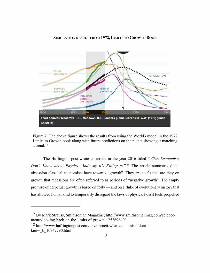
The World3 model described in the book is a system dynamics model of present

trends in a way of looking into the future, especially the very near future, and especially if

the quantity being considered is not much influenced by other trends that are occurring

elsewhere in the system. Of course, none of the five factors they were examining are

independent. Each of the 5 trends constantly interacts with each other like

• Population cannot grow without food

• Food production is increased by growth of capital

• More capital requires more resources

• Discarded resources become pollution

• Pollution interferes with the growth of both population and food

Furthermore, over long periods of time, each of these factors also feedbacks to

influence each other. Some projections from the 1972 book using the World3 model can

be seen below in Figure 2 along with the observed trends up until 2000.

13

SIMULATION RESULT FROM 1972, LIMITS TO GROWTH BOOK

Figure 2. The above figure shows the results from using the World3 model in the 1972

Limits to Growth book along with future predictions on the planet showing it matching

a trend.17

The Huffington post wrote an article in the year 2016 titled “What Economists

Don’t Know about Physics- And why it’s Killing us”.18 The article summarized the

obsession classical economists have towards “growth”. They are so fixated are they on

growth that recessions are often referred to as periods of “negative growth”. The empty

promise of perpetual growth is based on folly — and on a fluke of evolutionary history that

has allowed humankind to temporarily disregard the laws of physics. Fossil fuels propelled

17 By Mark Strauss, Smithsonian Magazine; http://www.smithsonianmag.com/science-

nature/looking-back-on-the-limits-of-growth-125269840/

18 http://www.huffingtonpost.com/dave-pruett/what-economists-dont-

know_b_10742790.html

14

the Industrial Revolution, which in turn gave us mechanization, rapid transportation, the

subjugation of nature, and industrial agriculture, all the ingredients for modern, urbanized,

high-density societies. Powered first only by coal, then oil came into the picture, and now

gas has joined the race, the world’s human population more than tripled between 1950 and

2010 (Figure 3).

Figure 3. World population 1750-2015 and projections until 2100.19

Thermodynamics refer to isolated, closed, and open systems. An isolated system is

hermetically sealed: it can exchange neither matter nor energy with its surroundings. At

the other extreme, an open system can exchange both. With a semi-permeable boundary, a

closed system, can exchange energy but not matter. Mainstream economists tend to think

19 https://ourworldindata.org/world-population-growth/#note-4

15

of the economy as an abstract, mathematical computerization independent of the physical

world. But economic activity necessarily requires natural resources, which are in limited

supply as discussed in the opening paragraph. The notion of perpetual economic growth is

absurd on face value because it demands an unbounded supply of natural resources and

thus an infinitely large earth.20

2.1.4. ECONOMIC MODELS AND DIFFERENT TYPES OF PRODUCTION FUNCTIONS

An Economic model (M. S. Morgan 2008) is a theoretical construct representing

economic processes by a set of variables and a set of logical and/or quantitative

relationships between them. It’s a simplified framework designed to illustrate the complex

process, often but not always using mathematical techniques. An economic model may

have various exogenous variables, and those variables may change to create various

responses by economic variables. Methodological uses of models include investigation,

theorizing, and fitting theories to the world (M. S. Morgan 2008). These models are used

for many purposes like forecasting, economic policy, planning and allocation, logistics,

business management etc.

Economic models can be such powerful tools in understanding some economic

relationships that it is easy to ignore their limitations (Stanford 1993).

The fundamental issue is circularity: embedding one's assumptions as foundational

"input" axioms in a model, then proceeding to "prove" that, indeed, the model's "output"

supports the validity of those assumptions. Such a model is consistent with similar models

20 https://academic.oup.com/nsr/article/3/4/470/2669331/Modeling-sustainability-

population-inequality

16

that have adopted those same assumptions. But is it consistent with reality? As with any

scientific theory, empirical validation is needed, if we are to have any confidence in its

predictive ability. If those assumptions are, in fact, fundamental aspects of empirical

reality, then the model's output will correctly describe reality (if it is properly "tuned", and

if it is not missing any crucial assumptions). But if those assumptions are not valid for the

particular aspect of reality one attempts to simulate, then it becomes a case of "GIGO" –

Garbage In, Garbage Out".

2.1.4.1. SOLOW-SWAN MODEL OF ECONOMIC GROWTH

The Solow–Swan model (Solow 1956) is an exogenous growth model, an economic

model of long-run economic growth set within the framework of neoclassical economics.

It attempts to explain long-run economic growth by looking at capital accumulation, labor

or population growth, and increases in productivity commonly referred to as technological

progress. At its core, it is a neoclassical aggregate production function, usually of a Cobb–

Douglas type, which enables the model "to make contact with microeconomics”

(Acemoglu 2009). The model was developed independently by Robert Solow and Trevor

Swan in 1956 and superseded the post-Keynesian Harrod–Domar model (Harrod 1939)

and (Domar 1946) . In 1987 Solow was awarded the Nobel Prize in Economics for his

work. Today, economists use Solow’s sources-of-growth accounting to estimate the

separate effects on economic growth of technological change, capital, and labor.

17

Assumptions in the model:

The key assumption of the neoclassical growth model is that capital is subject to

diminishing returns in a closed economy.

1. Given a fixed stock of labor, the impact on output of the last unit of capital

accumulated will always be less than the one before.

2. Assuming for simplicity no technological progress or labor force growth,

diminishing returns implies that at some point the amount of new capital produced

is only just enough to make up for the amount of existing capital lost due to

depreciation (Acemoglu, 2009). At this point, because of the assumptions of no

technological progress or labor force growth, we can see the economy ceases to

grow.

3. Assuming non-zero rates of labor growth complicates matters somewhat, but the

basic logic still applies (Solow 1956) in the short-run, the rate of growth slows as

diminishing returns take effect and the economy converges to a constant "steady-

state" rate of growth (that is, no economic growth per-capita).

4. Including non-zero technological progress is very similar to the assumption of non-

zero workforce growth, in terms of "effective labor": a new steady state is reached

with constant output per worker-hour required for a unit of output. However, in this

case, per-capita output grows at the rate of technological progress in the “steady-

state” (Swan 1956) (that is, the rate of productivity growth).

18

The Solow-Swan model (Solow 1956) is set in a continuous-time world with no

government or international trade. There is only one commodity, output as a whole, whose

rate of production is designated 𝑌(𝑡). Thus we can speak unambiguously of the

community’s real income. Part of each instant’s output is consumed and the rest is saved

and invested. The fraction of output saved is a constant 𝑠, so that the rate of saving is

𝑠𝑌(𝑡). The community’s stock of capital 𝐾(𝑡) takes the form of an accumulation of the

composite commodity. Net investment is then just the rate of increase of this capital stock

𝑑𝐾

𝑑𝑡 𝑜𝑟 �̇� , so we have the basic identity at every instant of time:

�̇� = 𝑠𝑌 Eq 1

The output is produced with the help of two factors of production, capital, and labor,

whose rate of input is 𝐿(𝑡). Technological possibilities are represented by a production

function

𝑌 = 𝐹(𝐾, 𝐿) Eq 2

The output is to be understood as net output after making good the depreciation of

capital. About production, all we will say at the moment is that it shows constant returns

to scale. Hence the production function is homogeneous of the first degree. This amount to

assuming that there is no scarce non-augmentable resource like land. Constant returns to

scale seem the natural assumption to make in a theory of growth. The scarce-land case

would lead to decreasing returns to scale in capital and labor.

Inserting (Eq 2) in (Eq 1) we get

�̇� = 𝑠𝐹(𝐾, 𝐿) Eq 3

19

This is one equation in two unknowns. One way to close the system would be to

add a demand-for-labor equation: marginal physical productivity of labor equals real wage

rate; and a supply-of-labor equation. The latter could take the general form of making labor

supply a function of the real wage equal to a conventional subsistence level. In any case,

there would be three equations in the three unknowns 𝐾, 𝐿, 𝑟𝑒𝑎𝑙 𝑤𝑎𝑔𝑒.

Instead, if we proceed more in the spirit of the Harrod’s model (Harrod 1939). As

a result of exogenous population growth, the labor force increases at a constant relative

rate 𝑛. In the absence of technological change 𝑛 is Harrod’s natural rate of growth. Thus

𝐿(𝑡) = 𝐿𝑜𝑒𝑛𝑡 Eq 4

Alternatively, (Eq 4) can also be looked as a supply curve of labor. It says that the

exponentially growing labor force is offered for employment completely in-elastically. The

labor supply curve is a vertical line which shifts to the right in time as the labor force grows

according to (Eq 4). Then the real wage adjusts so that all available labor is employed, and

the marginal productivity equation according to (Eq 5) and (Eq 6) determines the wage rate

which will actually rule.

𝜕𝐹

𝜕𝐿=

𝑤

𝑝 Eq 5

𝜕𝐹

𝜕𝐾=

𝑞

𝑝 Eq 6

In (Eq 3) 𝐿 stands for total employment whereas in (Eq 4) 𝐿 stands for the available

supply of labor. By identifying the two we are assuming that full employment is perpetually

maintained. When we insert (Eq 4) in (Eq 3) to get

20

�̇� = 𝑠𝐹(𝐾, 𝐿𝑜𝑒𝑛𝑡) Eq 7

We have this basic equation that determines the time evolution of capital

accumulation that must be followed if all available labor is to be employed. In summary,

(Eq 5) is a differential equation in the single variable 𝐾(𝑡). Its solution gives the only time

profile of the community’s capital stock that can fully employ the available labor. Once we

know the time evolution of capital stock and that of the labor force, we can compute from

the production function the corresponding time path of real output.

2.1.4.2. COBB-DOUGLAS MODEL OF PRODUCTION

In economics, the Cobb–Douglas (Cobb and Douglas 1928) and (Douglas 1976)

production function is a particular functional form of the production function, widely used

to represent the technological relationship between the amounts of two or more inputs,

particularly physical capital and labor, and the amount of output that can be produced by

those inputs. Sometimes the term has a more restricted meaning, requiring that the function

display constant returns to scale (in which case 𝛽 = 1 − 𝛼 in the formula below). In its

most standard form for production of a single good with 2 factors, the function is

𝑌 = 𝐴𝐿𝛽𝐾𝛼 Eq 8

Where,

𝑌 = 𝑇𝑜𝑡𝑎𝑙 𝑝𝑜𝑑𝑢𝑐𝑡𝑖𝑜𝑛 ( 𝑡ℎ𝑒 𝑟𝑒𝑎𝑙 𝑣𝑎𝑙𝑢𝑒 𝑜𝑓 𝑎𝑙𝑙 𝑔𝑜𝑜𝑑𝑠 𝑝𝑟𝑜𝑑𝑢𝑐𝑒𝑑 𝑖𝑛 𝑎 𝑦𝑒𝑎𝑟)

𝐿 = 𝐿𝑎𝑏𝑜𝑟 𝐼𝑛𝑝𝑢𝑡 ( 𝑡ℎ𝑒 𝑡𝑜𝑡𝑎𝑙 𝑛𝑢𝑚𝑏𝑒𝑟 𝑜𝑓 𝑝𝑒𝑟𝑠𝑜𝑛𝑠 − ℎ𝑜𝑢𝑟𝑠 𝑤𝑜𝑟𝑘𝑒𝑑 𝑖𝑛 𝑎 𝑦𝑒𝑎𝑟)

𝐾 = 𝐶𝑎𝑝𝑖𝑡𝑎𝑙 𝑖𝑛𝑝𝑢𝑡 ( 𝑡ℎ𝑒 𝑟𝑒𝑎𝑙 𝑣𝑎𝑙𝑢𝑒 𝑜𝑓 𝑎𝑙𝑙 𝑚𝑎𝑐ℎ𝑖𝑛𝑒𝑟𝑦,

𝑒𝑞𝑢𝑖𝑝𝑚𝑒𝑛𝑡, 𝑎𝑛𝑑 𝑏𝑢𝑖𝑙𝑑𝑖𝑛𝑔𝑠)

21

𝐴 = 𝑡𝑜𝑡𝑎𝑙 𝑓𝑎𝑐𝑡𝑜𝑟 𝑝𝑟𝑜𝑑𝑢𝑐𝑡𝑖𝑣𝑖𝑡𝑦

𝛼 𝑎𝑛𝑑 𝛽 𝑎𝑟𝑒 𝑡ℎ𝑒 𝑜𝑢𝑡𝑝𝑢𝑡 𝑒𝑙𝑎𝑠𝑡𝑖𝑐𝑖𝑡𝑖𝑒𝑠 𝑜𝑓 𝑐𝑎𝑝𝑖𝑡𝑎𝑙 𝑎𝑛𝑑 𝑙𝑎𝑏𝑜𝑟, 𝑟𝑒𝑠𝑝𝑒𝑐𝑡𝑖𝑣𝑒𝑙𝑦.

If

𝛼 + 𝛽 = 1, Eq 9

The production function has constant returns to scale, meaning that doubling the usage of

capital K and Labor L will also double output Y. If

𝛼 + 𝛽 < 1, Eq 10

Returns to scale are decreasing, and if

𝛼 + 𝛽 > 1, Eq 11

Returns to scale are increasing. Assuming perfect competition21 and 𝛼 + 𝛽 = 1, 𝛼 𝑎𝑛𝑑 𝛽

can be shown to be capital’s and labor’s share of output.

2.1.4.3. LEONTIEF PRODUCTION FUNCTION

The Leontief production function or fixed proportions production function is a

production function that implies the factors of production will be used in fixed

(technologically pre-determined) proportions, as there is no substitutability between

factors. It was named after Wassily Leontief and represents a limiting case of the constant

21 http://economictimes.indiatimes.com/definition/perfect-competition

22

elasticity of substitution production function (Arrow, et al. 1961), (Jorgensen 2000) and

(Klump, William and McAdam 2007)

For the simple case of a good that is produced with two inputs, the function is of

the form

𝑞 = 𝑀𝑖𝑛(𝑧1

𝑎,

𝑧2

𝑏) Eq 12

where q is the quantity of output produced, z1 and z2 are the utilized quantities of

input 1 and input 2 respectively, and a and b are technologically determined constants.

2.2. GAPS IN LITERATURE

All economic models, no matter how complicated, are subjective approximations

of reality designed to explain observed phenomena. It follows that the model’s predictions

must be tempered by the randomness of the underlying data it seeks to explain and by the

validity of the theories used to derive its equations. A good example would be highlighting

the failure of existing models to predict or untangle the reasons for the global financial

crisis that began in 2008. Insufficient attention to the links between overall demand, wealth,

and in particular excessive financial risk taking has been blamed.22 No economic model

can be a perfect description of reality. Economic models can also be classified in terms of

the regularities they are designed to explain or the questions they seek to answer. For

example, some models explain the economy’s ups and down around an evolving long-run

path, focusing on the demand for goods and services without being too exact about the

sources of growth in the long run. Other models are designed to focus on structural issues,

22 http://www.imf.org/external/pubs/ft/fandd/basics/models.htm

23

such as the impact of trade reforms on long-term production levels, ignoring short term

oscillations.

Keynesian economics tells us that how in the short run, and especially during

recessions, economic output is strongly influenced by aggregate demand.23 In the

Keynesian view, aggregate demand does not necessarily equal the productive capacity of

the economy; instead, it is influenced by a host of factors and sometimes behaves

erratically, affecting production, employment, and inflation. The theories forming the basis

of Keynesian economics were first presented by the British economist John Maynard

Keynes during the Great Depression in his 1936 book, “The General Theory of

Employment, Interest, and Money” (Keynes 1936). Keynesian economists often argue

that private sector decisions sometimes lead to inefficient macroeconomic outcomes which

require active policy responses by the public sector, in particular, monetary policy actions

by the central bank and fiscal policy actions by the government, in order to stabilize output

over the business cycle. Keynesian economics advocates a mixed economy –

predominantly private sector, but with a role for government intervention during

recessions. Keynesian economics served as the standard economic model in the developed

nations during the latter part of the Great Depression, World War II, and the post-war

economic expansion (1945–1973), though it lost some influence following the oil shock

and resulting stagflation of the 1970’s. The advent of the financial crisis of 2007–08 caused

a resurgence in Keynesian thought, which continues as new Keynesian economics (Dixon

1999).

23 http://www.imf.org/external/pubs/ft/fandd/2014/09/basics.htm

https://en.wikipedia.org/wiki/Private_sector

https://en.wikipedia.org/wiki/Public_sector

https://en.wikipedia.org/wiki/Monetary_policy

https://en.wikipedia.org/wiki/Central_bank

https://en.wikipedia.org/wiki/Fiscal_policy

https://en.wikipedia.org/wiki/Business_cycle

https://en.wikipedia.org/wiki/Mixed_economy

24

Steve Keen is a professor of Economics at Kingston University London who writes

a blog called Steve Keen’s Debtwatch where he wrote an article titled “Neoclassical

Economics: mad, bad and dangerous to know”, which was published in 2009 (Keen,

Neoclassical Economics: mad, bad, and dangerous to know 2009). In this article, he

highlights how the most important thing that global financial crisis has done for economic

theory is to show that neoclassical economics is not merely wrong, but dangerous. He

justifies this by arguing how neoclassical economics contributed directly to the 2007-08

crisis by promoting a faith in the innate stability of a market economy, in a manner which

in fact increased the tendency to instability of the financial system, with its false belief that

all instability in the system can be traced to interventions in the market, rather than the

market itself, it championed the deregulation of finance and a dramatic increase in income

inequality. Its equilibrium vision of the functioning of finance markets led to the

development of the very financial products that are now threatening the continued

existence of capitalism itself.

Simultaneously it distracted economists from the obvious signs of an impending

crisis—the asset market bubbles, and above all the rising private debt that was financing

them. Paradoxically, as capitalism’s “perfect storm” approached, neoclassical

macroeconomists were absorbed in smug self-congratulation over their apparent success

in taming inflation and the trade cycle, in what they termed “The Great Moderation”.

25

3. Chapter 3: Research Approach

3.1. RESEARCH APPROACH

All models are wrong, and some are useful. The neoclassical economic framework

has proved useful for many purposes. But today’s challenges are those of new constraints

pushing the boundaries of economic thinking. Central banking interest rates are lower (now

negative in some cases) than any time in the history of central banking, and debt levels are

at all-time highs. Also, global food and energy are no longer getting cheaper (King 2015b)

after continuous decreases since the industrial revolution. Narratives and models exist for

describing past agrarian civilizations and their relation to resource access (J. A. Tainter,

The Collapse of Complex Societies 1988), (J. A. Tainter, Energy, Complexity, and

Sustainability: A Historical Perspective 2011) and (Tainter, et al. 2003) as well dynamics

of population and social structure (Turchin, Currie, et al. 2013) and (Turchin and Nefedov,

Secular Cycles 2009) These narratives often describe how the quality and quantity of

natural resources relate to the cyclical growth, structure, inequality, and/or complexity of

society and/or the economy overall.

However, it is unclear how these narratives translate both to today’s modern society

enabled by fossil fuels and to a low-carbon energy economy transition. Past agricultural

societies rose and fell powered essentially by renewable energy flows (e.g., sunlight).

These societies were also very unequal with a small number of elite collecting the vast

majority of the income while the vast majority of commoners worked in the energy and

food (e.g., agricultural) sectors. Fossil-fueled machinery, fertilizers, and irrigation enabled

energy and food costs to continually decrease since the start of industrialization. Thus,

today developed economies, primarily powered by fossil fuel stocks, have a very small

26

proportion of workers in energy and food sectors with an equal income and resource access

as compared to the preindustrial world (Mitchell 2013). If the food and energy costs have

reached their cheapest points then many current macroeconomic modeling approaches,

often calibrated only to relatively recent fossil-fueled history, might be insufficient for

understanding current and future economic growth with regard to constraints within food,

water, and energy sectors; climate change; and debt (Pindyck 2013), (Stern 2013) and

(Keen, A Monetary Minsky Model of the Great Recession 2013a). As we attempt to

transition to a low-carbon energy supply, largely based on renewable energy flows, it is

paramount to have internally consistent macro-scale models that track flows and

interdependencies among money, debt, employment and biophysical quantities (e.g.,

natural resources and population).

What if you realized that the fundamental economic framework of models that are

meant to guide a low-carbon energy transition prevents them from actually answering the

question they are supposed to answer? Instead of assuming a series of energy investments,

and then estimating the economic impacts of those choices, they actually do the exact

opposite. They assume economic growth and then make a series of investments to meet

emissions targets without actually factoring in how the energy systems themselves

feedback to economic growth or other social goals.

Monetary models of finance and debt assume that energy resources and technology

are not constraints on the economy. Energy transition scenario models assume that

economic growth, finance, and debt will not be constraints on the energy transition. These

assumptions must be eliminated, and the modeling concepts must be integrated if we are

27

to properly plan for and understand the dynamics of a low-carbon and/or renewable energy

transition.

Over the past 200 years, human civilization has transformed from one dependent

upon renewable energy flows (e.g., sunlight) to one dependent upon fossil energy stocks

(e.g., oil, gas, and coal). Climate change and resource depletion are driving society to

understand how to again live off of low-carbon renewable flows of primary energy. Except

for this time, we are much smarter, and we have increased technological know-how.

As we attempt to transition to a low-carbon energy supply, largely again based

again on renewable energy flows, it is paramount to have internally consistent macro-scale

models that track flows and interdependencies among money, debt, employment and

biophysical quantities (e.g., natural resources and population). This research objective is to

develop a framework to describe our contemporary and future macroeconomic situation

that is consistent with both biophysical and economic principles. Unfortunately, this

fundamental integration does not underpin our current thinking. This improved framework

can contribute to more robust policy-making ability under both current and future changing

circumstances.

The objective here is to develop a consistent biophysical and economic framework

to describe the industrial transition to our contemporary macroeconomic state. This

research seeks to integrate macro-scale system dynamics models of money, debt, and

employment (specifically the Goodwin and Minsky models of (Keen, Finance and

Economic Breakdown: Modeling Minsky's "Financial Instability Hypothesis" 1995) ) with

system dynamics models of biophysical quantities (specifically population and natural

resources such as in (Meadows, et al. 1972) and (Motesharrei, Rivas and Kalnay 2014). In

28

other words, there are models of each separately, but they have not been combined to

fundamentally link the biophysical world to monetary frameworks. Figure 4 outlines the

approach as a critical extension of existing literature.

This type of modeling can answer important questions for a low-carbon transition

(two examples):

1. How does the rate of transition feedback to the growth of population, economic

output, and debt?

The faster we transition, the more capital, labor, and natural resources will be

mobilized to become part of the “energy” sectors. The larger this mobilization, the higher

the cost of energy will become as there is an increasing number of “energy” sector workers

dependent upon selling energy to a decreasing set of “non-energy” sector consumers.

Increasing labor and capital shares for energy is the exact opposite trend of industrialization

as we know it, and there is a critical need to understand the associated feedbacks. For

example, the most recent oil and gas boom and bust cycle could possibly be explained by

too many resources being allocated to the energy sector over too short of a time for the rest

of the economy to adjust. It is important we understand this growth feedback between the

size (labor, capital, energy) of energy and food sectors and economic growth.

2. How do the capital structure (e.g., fixed costs versus variable costs) of fossil and

renewable energy systems relate to and affect economic outcomes?

Renewable and low-carbon energy systems (e.g., PV, the wind, nuclear,

electrochemical storage) are characterized by a much higher fraction of fixed (capital) costs

as compared to fossil energy systems (e.g., coal, natural gas, and oil). Higher fixed costs

29

systems are more favorable in certain (e.g., predictable) and lower growth (with low

discount rate) environments whereas lower fixed cost systems are more favorable in

uncertain and high growth situations (Chen 2016). The reason is that in high growth

situations you do not want to be “stuck” with old capital in which you are still waiting for

returns to reinvest. Low economic growth, associated with low discount rates, also make

high fixed cost and longer-life assets, like renewable systems, more favorable. Thus, we

should expect low growth (“secular stagnation”) to be associated with low-interest rates

and high renewable energy installations, just as has happened over the last several years.

30

RESEARCH APPROACH

Figure 4. The research approach will focus to make a critical link between biophysical

modeling concepts and those of economic models that specifically include the link of

debt-based finance to employment and economic growth.

31

3.2. BACKGROUND AND CONTEXT

3.2.1. LOTKA-VOLTERRA-PREDATOR-PREY MODEL

The Predator–Prey model, was derived independently by two mathematicians

Alfred Lotka and Vito Volterra, in the early 20th century (Lotka 1925). This model

describes the dynamics of competition between two species, say, wolves and rabbits. The

governing system of equations is

𝑑𝑥

𝑑𝑡= (𝑎𝑦)𝑥 − 𝑏𝑥 Eq 13

𝑑𝑦

𝑑𝑡= 𝑐𝑦 − (𝑑𝑥)𝑦 Eq 14

In the above system, x represents the predator (wolf) population; y represents the

prey (rabbit) population; a determines the predator's birth rate, i.e., the faster growth of

wolf population due to availability of rabbits; b is the predator's death rate; c is the prey's

birth rate; d determines the predation rate, i.e., the rate at which rabbits are hunted by

wolves. Rather than reaching a stable equilibrium, the predator and prey populations show

periodic, out-of-phase variations about the equilibrium values

𝑥𝑒 =𝑐

𝑑 Eq 15

𝑦𝑒 =𝑏

𝑎 Eq 16

Note the consistency of the units on the left and right-hand sides of Eq 13 through

Eq 16. A typical solution of the predator–prey system can be seen in Figure 5.

32

Figure 5. A typical solution of the predator-prey system (Motesharrei, Rivas and Kalnay

2014, 3) obtained by running the system with a certain set of initial conditions for the

number of wolves and rabbits at the start of the simulation.

3.2.2. MULTIPLIER-ACCELERATOR MODEL

The Multiplier-Accelerator (Samuelson 1939) Interaction Theory came into

existence when the theorist of the Keynesian tradition stresses on multiplier process in

economic fluctuations while J.K. Clark emphasized on the role of acceleration in the

business fluctuations.

But however, Paul Samuelson, the post-Keynesian business cycle theorists asserted

that neither the multiplier theory nor the principle of acceleration alone is adequate to

analyze the business cycle fluctuations. And hence, proposed the Multiplier-Accelerator

Model, also called as Hanson-Samuelson Model.

The multiplier-Accelerator model is based on the Keynesian multiplier, a

consequence of the assumption that the level of economic activity decides the consumption

33

intentions and the accelerator theory of investment which is based on the assumption that

the investment intentions depend on the pace with which the economic activities grow.

The Samuelson’s model is the first step towards integrating the theory of multiplier

and principle of acceleration. This theory shows how well these two tools are integrated to

generate income, so as to have an increased consumption and investment demands more

than expected and how these reflect the changes in the business cycle. To understand

Samuelson’s model one needs to know the difference between the Autonomous and

Derived Investments.

Autonomous investment is the investment undertaken due to the external factors

such as new inventions in technology, production process, production methods, etc. While,

the Derived Investment is the investment, particularly in capital equipment, is undertaken

to meet the increase in consumer demand necessitating new investment.

With an increase in the autonomous investment, the income of people rises and the

process of multiplier begins. With increased incomes, the demand for the consumer goods

also increases depending on the marginal propensity to consume. And if the firm has no

excess production capacity, then its existing capital will stand inadequate to meet the

increased demand. Therefore, the firm will undertake new investment to meet the growing

demand. Thus, an increase in consumption creates a demand for investment, and this is

called as Derived Investment. This marks the beginning of the acceleration process.

When the derived investment takes place, the income rises, in the same manner, it

does when the autonomous investment took place. With an increased income, the demand

for the consumer goods also increases. This is how, the multiplier process and principle of

acceleration interact with each other, such that income grows at a faster rate than expected.

34

In short, the exogenous factors (external origin) lead to autonomous investment,

which results in the multiplier effect. This multiplier effect creates the derived investment,

which results in the acceleration of investment. Samuelson made the following

assumptions in the analysis of this interaction process:

1. There is no excess production capacity.

2. At least one-year lag in the consumption.

3. At least one-year lag in the increase in demand for consumption and

investment.

4. No government intervention, and no foreign trade.

Samuelson’s model of business fluctuations is presented below:

Given the assumption (4) as above, the economy is said to be in equilibrium

when,

𝑌𝑡 = 𝐶𝑡 + 𝐼𝑡 Eq 17

Where, 𝑌𝑡= national income, 𝐶𝑡 = total consumption expenditure, 𝐼𝑡 = total investment

expenditure, all in a period ‘t’.

Given the assumption (2) as above, the consumption function can be expressed as

𝐶𝑡 = 𝑎𝑌𝑡−1 Eq 18

Where, 𝑌𝑡−1= income in period t-1, and a = marginal propensity to consume

Investment is a function of consumption with one year lag, and is expressed as:

35

𝐼𝑡 = 𝑏(𝐶𝑡 − 𝐶𝑡−1) Eq 19

Where, b = capital/output ratio. Here parameter ‘b’ determines the accelerator.

By substituting equation (Eq 18) for 𝐶𝑡 and equation (Eq 19) for 𝐼𝑡, the equilibrium

equation can be written as:

𝑌𝑡 = 𝑎𝑌𝑡−1 + 𝑏(𝑎𝑌𝑡−1 − 𝑎𝑌𝑡−2) Eq 20

Further, simplifying the equation:

𝑌𝑡 = 𝑎(1 + 𝑏)𝑌𝑡−1 − 𝑎𝑏𝑌𝑡−2 Eq 21

Samuelson’s model suffers from the following criticisms:

1. The critics feel that it is far too simple a model to explain what all happens during

the economic fluctuations. They are of an opinion that the model has been

developed on highly simplifying assumptions.

2. Samuelson stresses on the role of multiplier and accelerator and the interaction

between them as a fundamental cause of business fluctuations. Thus, like other

theories, it has also ignored the other important factors that play a crucial role in a

cyclical process, such as producer’s expectations, change in the psychology of

businessmen, change in consumer’s tastes and preferences and the exogenous

factors.

3. One of the major criticism of this model is that it is assumed that the capital/output

ratio remains constant while there are chances of change in this ratio during

expansion and depression.

36

4. Finally, the cyclical patterns suggested in this model do not confirm the real-world

experience.

In spite of these bottlenecks, a Samuelson’s model is acclaimed as a sound attempt

to integration between the Keynesian multiplier theory and Clarke’s acceleration principle,

that fairly explains the causes of fluctuations in the business cycles.24

3.2.3. THE GOODWIN MODEL25,26

In 1967, Richard Goodwin developed an elegant model meant to describe the

evolution of distributional conflict in growing, advanced capitalist economies. The

Goodwin model is important because it tells a story about the dynamics of the growth and

distribution process at the heart of the Foley and Michl approach (Foley and Michl 1999).

The key variables in the Goodwin model are the share of labor in national income,

and the employment rate. In the conventional wage share model of Foley and Michl, the

labor share is always constant at its conventional level. While this is a reasonable

approximation over the very long-run, the labor share fluctuates in actual economies

(Goodwin 1967). Similarly, in the conventional wage share model, the amount of labor

hired each period is given by ρK/x where ρ is the output/capital ratio, x is labor

productivity, and K is capital.

24 Luca Fiorito "John Maurice Clark's Contribution to the Genesis of the Multiplier

Analysis," University of Siena Dept. of Econ. Working Paper No. 322

25 http://www.danieletavani.com/wp-content/uploads/2014/05/ECON705_Goodwin.pdf

26 http://orion.math.iastate.edu/driessel/14Models/1967growth.pdf

37

The economic intuition is the following: Suppose the economy is expanding, and

employment increases. Higher labor demand generates wage inflation which, as long as

real wages increase more than labor productivity, increases the wage share in output. If

consistently with the Classical view, workers do not save, the resulting decrease in the

profit share will act in reducing future investment and output. But then the economy is

down, and lower demand for labor will then correspond to lower output, leading the way

to lower wage inflation or even wage deflation. The labor share will decrease. But a higher

profit share will produce a surge in investment, which will generate higher employment,

thus improving workers bargaining power and consequently wages. At this point, the wage

share has increased, and the cycle can repeat itself.

Goodwin realized that this type of dynamics is also found in simple biological

systems, such as the Lotka-Volterra Predator-Prey model described in Section 3.2.1.

Suppose that in a certain territory there is a predator species and a prey species. If predators

are too little in number, Prey’s will proliferate, thus pushing against the resource constraint

in the territory. Prey proliferation, however, makes predators' life easier: they will be better

fed and reproduce at a higher rate. But when the number of predators is too high, finding

preys to eat becomes harder, and mortality among predators will increase. Prey’s will have

more opportunities to reproduce, and the cycle can repeat itself.

38

Assumptions in the model

1. steady technical progress (disembodied);27

2. steady growth in the labor force;

3. only 2 factors of production, labor and “capital” (plant and equipment), both

homogeneous and non-specific;

4. all quantities real and net;

5. all wages consumed;

6. all profits saved and invested;

These assumptions are of a more empirical, and disputable, sort:

7. a constant capita-output ratio;

8. a real wage rate which rises in the neighborhood of full employment

3.2.3.1. MATHEMATICS OF GOODWIN MODEL

Goodwin’s model can be expressed as 2 differential equations in the rate of

employment and the wages share of output. (Keen, A Monetary Minsky Model of the Great

Moderation and the Great Recession 2013) outlines it in terms of absolute values, since

this is the form in which the final monetary Minsky model in this research is also expressed

as also in Keen’s 2013 paper. The economy is populated by workers and capitalists.

Workers supply labor services to firms owned by capitalists, who do not save and consume

27 Disembodied Technical Progress: Improved technology which allows increase in the

output produced from given inputs without investing in new equipment.

39

all of their income. Capitalists own capital assets, consume and save. The aggregate output

is denoted by Y, capital by K and labor by L. Labor is homogeneous, hence a single wage

rate w can be used. Production of output occurs with the following fixed proportions for

technology:

𝑌 = min {𝐾

𝑣, 𝑎𝐿} Eq 22

Implying that the real unit labor cost which is the labor share can be represented as

𝑤

𝑎 . Labor productivity grows at the exogeneous rate α>0, while the capital to output ratio

remains constant over time. The model also assumes a exogenous growth of the labor force,

at a rate β>0. Since full employment might or might not occur, we denote the employment

rate by λ = L/N, where N is the total population/ labor force in the model

Keen outlines Goodwin’s equation in terms of absolute values since this is the form

in which the final monetary Minsky model in his paper (Keen, 2013) is expressed. The

basic deterministic casual cycle of the model is:

1. The level of capital stock K determines the level of output per annum Y via the

accelerator v:

𝑌 =𝐾

𝑣 Eq 23

2. The level of output determines the level of employment L via labor productivity a:

𝐿 =𝑌

𝑎 Eq 24

3. The level of employment determines the employment rate λ (the ratio of L to

population N):

𝜆 =𝐿

𝑁 Eq 25

40

4. The employment rate determines the rate of change of real wages w via a Phillips

curve:

1

𝑤

𝑑𝑤

𝑑𝑡= −𝑐 + 𝑑𝜆 Eq 26

5. Profit determines investment I (in the Goodwin model, all profits are invested):

I = ∏ Eq 27

6. Investment minus depreciation γ determines the rate of change of capital stock K,

closing the model:

𝑑𝐾

𝑑𝑡= 𝐼 − 𝛾. 𝐾 Eq 28

With population growth of 𝛽 percent per annum, labor productivity growth of 𝛼

percent per annum, and a linear Phillips curve relation of the form (−𝑐 + 𝑑𝜆) (where c

and d are constants) (Phillips 1958), the model consists of the following 4 differential

equations in the level of employment, the real wage, labor productivity and population

growth. A typical simulation of the Goodwin model can be seen in Figure 6.

1. 𝑑𝐿

𝑑𝑡= 𝐿(

(1−𝑤

𝑎)

𝑣− 𝛾 − 𝛼) Eq 29

2. 𝑑𝑤

𝑑𝑡= (−𝑐 + 𝑑𝜆)𝑤 Eq 30

3. 𝑑𝑎

𝑑𝑡= 𝛼𝑎 Eq 31

4. 𝑑𝑁

𝑑𝑡= 𝛽𝑁 Eq 32

Eq 29 can also be modeled in other forms where it can be represented as Eq 33 &

Eq 34 below in accord with the condition in Eq 22 when Y =𝐾

𝑣= 𝑎𝑙 under full capital

41

utilization (Keen, Finance and Economic Breakdown: Modeling Minsky's "Financial

Instability Hypothesis" 1995) and therefore,

𝑑𝑌

𝑑𝑡= 𝑌. (

(1−𝑤

𝑎)

𝑣− 𝛾) Eq 33

and,

𝑑𝐾

𝑑𝑡= 𝐾. (

(1−𝑤

𝑎)

𝑣− 𝛾) Eq 34

42

SIMULATION RESULTS FROM THE GOODWIN MODEL

Figure 6. Goodwin model with the Linear form for the Phillips curve (-c + d λ) where c =

4.8 and d =5 are constants and λ is the employment rate with an initial value of 0.97. The

initial value for the real wage rate 𝑤 is equal to 0.88 and that for the labor productivity 𝑎

is equal to 1.

43

3.2.4. HUMAN AND NATURE DYNAMICS (“HANDY”): MODELING INEQUALITY AND

USE OF RESOURCES IN THE COLLAPSE OR SUSTAINABILITY OF SOCIETIES

3.2.4.1. THE MODEL

The HANDY model (Motesharrei, Rivas and Kalnay 2014) is inspired from the

predator – prey model where instead of modeling two different species we have

1. The human population which comprises of the elites and commoners in the

model and

2. The available nature which is the total nature available in the system which is

consumed by the population in the model.

The HANDY paper defines the population to address the effect of inequality

towards the sustenance of a particular society. There are 4 basic equations which describe

the entire idea:

1. State Variables

a. Population of commoners (𝑥𝑐)

b. Population of elites (𝑥𝑒)

c. Nature (y)

d. Wealth (w)

2. State equations

a. Rate of change of commoner’s population

𝑑

𝑑𝑡𝑥𝑐 = 𝛽𝑐𝑥𝑐 − 𝛼𝑐𝑥𝑐 Eq 35

b. Rate of change of elite’s population

𝑑

𝑑𝑡𝑥𝑒 = 𝛽𝑒𝑥𝑒 − 𝛼𝑒𝑥𝑒 Eq 36

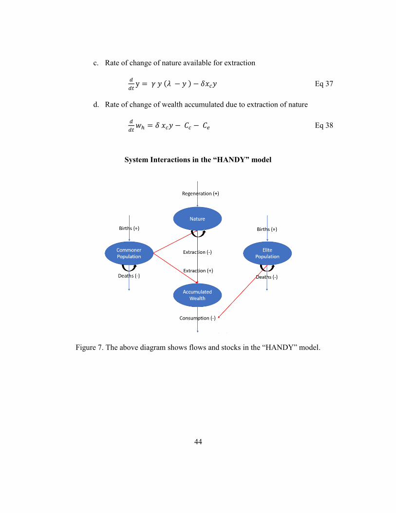
44

c. Rate of change of nature available for extraction

𝑑

𝑑𝑡y = 𝛾 𝑦 (𝜆 − 𝑦 ) − 𝛿𝑥𝑐𝑦 Eq 37

d. Rate of change of wealth accumulated due to extraction of nature

𝑑

𝑑𝑡𝑤ℎ = 𝛿 𝑥𝑐𝑦 − 𝐶𝑐 − 𝐶𝑒 Eq 38

System Interactions in the “HANDY” model

Figure 7. The above diagram shows flows and stocks in the “HANDY” model.

45

Assumptions in the model:

1. The population grows through a birth rate β and decrease through a death rate α.

The birth rate β is considered the same for both the elites and the commoners in the

model.

2. The commoners are the only one’s working in the system towards extraction of

nature which in return gets stored as accumulated wealth which is the final thing

consumed by both the commoners and elites.

3. Both available nature and accumulated wealth have similar units called as eco$

4. Consumption by both commoners and elites are different with elites consuming

higher than the commoners by a factor κ. Their consumption is given by

a. 𝐶𝑐 = min (1,𝑤

𝑤𝑡ℎ) 𝑠𝑥𝑐 Eq 39

b. 𝐶𝑒 = min (1,𝑤

𝑤𝑡ℎ) 𝑠𝜅𝑥𝑒 Eq 40

𝑤𝑡ℎ = ρ(𝑥𝑐 + 𝜅𝑥𝑒) Eq 41

Eq 41 above is the wealth threshold value of wealth below which famine starts and

ρ is the minimum required consumption per capita. The death rates of both elites and

commoners are a function of their consumptions and expressed in terms of 𝑤

𝑤𝑡ℎ (Figure 8)

and the graphical representation of the death rates can be seen below in Figure 9.

c. 𝛼𝐶 = 𝛼𝑚 + max (0,1 −𝐶𝐶

𝑠𝑥𝐶)(𝛼𝑀 − 𝛼𝑚) Eq 42

d. 𝛼𝐸 = 𝛼𝑚 + max (0,1 −𝐶𝐸

𝑠𝜅𝑥𝐶)(𝛼𝑀 − 𝛼𝑚) Eq 43

46

Where,

𝐶𝑐 = 𝐶𝑜𝑛𝑠𝑢𝑚𝑝𝑡𝑖𝑜𝑛 𝑏𝑦 𝐶𝑜𝑚𝑚𝑜𝑛𝑒𝑟𝑠, 𝐶𝑒 = 𝐶𝑜𝑛𝑠𝑢𝑚𝑝𝑡𝑖𝑜𝑛 𝑏𝑦 𝐸𝑙𝑖𝑡𝑒𝑠

𝛼𝐶 = 𝐶𝑜𝑚𝑚𝑜𝑛𝑒𝑟 𝐷𝑒𝑎𝑡ℎ 𝑅𝑎𝑡𝑒, 𝛼𝑒 = 𝐸𝑙𝑖𝑡𝑒 𝐷𝑒𝑎𝑡ℎ 𝑅𝑎𝑡𝑒

𝛼𝑚 = 𝑁𝑜𝑟𝑚𝑎𝑙 (𝑚𝑖𝑛𝑖𝑚𝑢𝑚) 𝐷𝑒𝑎𝑡ℎ 𝑅𝑎𝑡𝑒, 𝛼𝑀 = 𝐹𝑎𝑚𝑖𝑛𝑒 (𝑚𝑎𝑥𝑖𝑚𝑢𝑚) 𝐷𝑒𝑎𝑡ℎ 𝑅𝑎𝑡𝑒

𝑤𝑖𝑡ℎ 𝑡ℎ𝑒 𝑐𝑜𝑛𝑑𝑖𝑡𝑖𝑜𝑛 𝑡ℎ𝑎𝑡

𝛼𝑚 < 𝛽𝑒 < 𝛽𝐶 < 𝛼𝑀 Eq 44

implying that the birth rates cannot be higher than the maximum death rate and less than

the minimum death rate in the model.

Figure 8. Consumption rates in HANDY.

Figure 9. Death rates in HANDY.

3.2.4.2. DIFFERENT SCENARIOS IN THE MODEL

Motesharrei et al. 2014 uses the HANDY model to explore different scenarios by

varying the factors (i) and (ii) below in order to explore different scenarios. They do this

47

in order to explore two different types of possible collapses in the society either due to

excess/rapid extraction of nature or high inequality in the society

(i) Rate of depletion of nature δ

(ii) Inequality Factor κ

One such scenario is of an Egalitarian society: An Egalitarian society in the paper

is defined as a society with no elites in the model and therefore 𝑥𝑒 = 0. Results from

simulating such scenarios can be seen in Figure 10 and Figure 11 with two different rates

for the depletion of nature δ. At lower values of δ the society reaches a steady state over a

long period of time. Whereas, at higher values a, collapse is seen in the society when the

population overshoots the carrying capacity in the model. The carrying capacity in the

model is defined as the maximum population the society can sustain after which it starts

falling due to lack of availability of nature. Another scenario that has been discussed in the

paper is of an Equitable Society Figure 12 and Figure 13 where both the elites and

commoners exist in the society but they both consume equally implying that 𝑥𝑒 ≠ 0 and κ

= 1. Similar results are seen as in an Egalitarian Society at different values of δ, where a

collapse is observed at higher values and a steady state at lower values. But in another case

when κ = 100 (Figure 15) which is the case in an Unequal Society in the paper, a collapse

is observed after an apparent equilibrium due to high inequality in the society. Whereas

even in an Unequal Society with lower value of κ = 10 (Figure 14) a steady state is reached

on a long run.

48

DIFFERENT SCENARIOS FROM “HANDY”

Figure 10. A soft landing to the optimal

equilibrium is observed in the figure where

the elite population in red is equal to zero

and the final population reaches the

maximum carrying capacity at a low value

of the rate of depletion of nature δ =6.67×10−6 Adapted from Motesharrei et

al., 2014.

Figure 11. An irreversible collapse is

observed in the figure where again the elite

population in red is equal to zero in an

egalitarian society. All the state variables

collapse to zero in this scenario due to over

depletion of nature at a higher value of the

rate of depletion of nature δ = 36.685×10−6.

Adapted from Motesharrei et al., 2014.

Figure 12. An equilibrium between both

Workers(Commoners) and Non-

Workers(Elites) can be attained with a low

value of the rate of depletion of nature δ =8.33×10−6. Adapted from Motesharrei et

al., 2014, 97.

Figure 13. Whereas an Irreversible collapse

in the society is observed at a higher value of

the rate of depletion of nature δ = 4.33×10−5.due to over depletion of nature.

Adapted from Motesharrei et al., 2014, 97.

49

Figure 14. With a moderate inequality c, the

states in the model reach an optimal

equilibrium at a relatively lower depletion

rate of nature δ = 6.35×10−6 and 𝑥𝑒 =3×10+3 Adapted from Motesharrei et al.,

2014, 98.

Figure 15. Population Collapse following an

apparent equilibrium due to a small initial

Elite population when κ =100 at a nature

depletion value of δ = 6.67×10−6 and 𝑥𝑒 =1×10−3 Adapted from Motesharrei et al.,

2014, 98.

3.2.4.3. SUMMARY

The model tries to highlight the history where the collapse of even advanced

civilizations has occurred over the past which was followed by centuries of population and

cultural decline and economic regression. The paper tries to explain this by building a

simple mathematical model to explore the essential dynamics of interaction between

population and natural resources. It also highlights the role inequality in a society plays

towards a sustainable future. The Human and Nature Dynamics (“HANDY”) was inspired

by the predator-prey model, with the human population acting as the predator and nature

the prey. To sum up the findings in the paper the 2 critical features that were apparent in

the historical societal collapses – over-exploitation of natural resources and strong

economic stratification can both independently lead to a collapse of the society.

50

3.2.5. A MONETARY MINSKY MODEL OF THE GREAT MODERATION AND THE GREAT

RECESSION

Hyman Minsky was an American economist, a professor of economics who

developed the financial instability hypothesis to address if the great depression could

happen again and if “It” can happen, why didn’t “It” occur in the years since World War

II? He advocated that to answer these questions it is necessary to have an economic theory

which makes great depressions one of the possible states in which our type of capitalist

economy can find itself. (Minsky,1982a, pg.5). Minsky instead combined insights from

Schumpeter, Fisher, and Keynes to develop a theory of financially driven business cycles

which can lead to an eventual debt-deflationary crisis. Steve Keen in his 1995 paper titled

“Finance and economic breakdown: modeling Minsky’s “financial instability

hypothesis”28 highlights that Minsky’s attempts to devise a mathematical model of his

hypothesis were unsuccessful (Minsk, 1957)29 arguably because the foundation he used the

multiplier-accelerator- model was itself flawed (Keen, 2000, pg.84-89). Keen 1995 (Keen,

1995, pg. 614-618) instead used Goodwin’s growth cycle model (Goodwin, 1967), which

generates a trade cycle with growth out of a simple deterministic structural model of the

economy as described earlier in section 3.2.3.

1. State Variables:

a. Output (Y)

b. Rate of change of real wages (w)

c. Debt (D)

d. Labor Productivity (a)

e. Population (N)

28 https://www.jstor.org/stable/4538470?seq=1#page_scan_tab_contents

29 The first of Minsky’s two papers in the AER set out a mathematical model of a

financially driven trade cycle developed during his Ph.D., but he never attempted to

develop the model further (Minsky,1957).

51

2. State equations:

a. The rate of change of Output:

𝑑𝑌

𝑑𝑡= 𝑌(

𝐼(∏

𝑣𝑌)

𝑣− 𝛾) Eq 45

b. The rate of change of real wage rate 𝑤 via Phillips curve:

𝑑𝑤

𝑑𝑡= 𝑝ℎ(𝜆)𝑤 Eq 46

c. The rate of change of Debt:

𝑑𝐷

𝑑𝑡= 𝐼 (

∏

𝑣𝑌) Y- ∏ Eq 47

d. The Rate of change of Labor Productivity 𝑎 at a constant rate of growth 𝛼:

𝑑𝑎

𝑑𝑡= 𝛼𝑎 Eq 48

e. The Rate of change in population N at a constant rate of growth 𝛽:

𝑑𝑁

𝑑𝑡= 𝛽𝑁 Eq 49

52

SYSTEM INTERACTIONS IN KEEN 2013, “GOODWIN WITH DEBT” MODEL

Figure 16. The above diagram shows the different interactions of different parameters in

the model.

One of the modifications made by Keen in modeling Minsky’s insights considering

the role of debt finance was to replace the what he calls the unrealistic linear function for

investment where all profits are invested in a linear relationship of Investments = Profits

with a nonlinear relation as in Eq 51, so that when the desire to invest exceeds retained

earnings, firms will borrow to finance investment. An exponential function for the

propensity to invest captures the most fundamental of Keynes’s insights about the behavior

of agents under uncertainty. Thus, desired investment exceeds profits at high rates of profit,

and is less than profit at low rates, because agents extrapolate current conditions into the

53

future. Similarly, with a nonlinear Phillips curve as in Eq 52, wages rise rapidly at high

levels of employment and fall slowly at lower levels.

Both the non-linear investment function (Figure 17) and the non-linear Phillips

curve (Figure 18) is obtained by substituting values defined in the Eq 51 and Eq 52 below

into the general expression format defined in (Keen, A Monetary Minsky Model of the

Great Moderation and the Great Recession 2013, 225) Eq 50.

𝐺𝑒𝑛𝐸𝑥𝑝(𝑥, 𝑥𝑣𝑎𝑙 , 𝑦𝑣𝑎𝑙 , 𝑠, 𝑚𝑖𝑛) = (𝑦𝑣𝑎𝑙 − min )𝑒(

𝑠

(𝑦𝑣𝑎𝑙−min ))(𝑥−𝑥𝑣𝑎𝑙)

+ 𝑚𝑖𝑛 Eq 50

Investment Function 𝐼(𝜋𝑟) = 𝐺𝑒𝑛𝐸𝑥𝑝(𝜋𝑟 , 0.05,0.05,1.75,0) Eq 51

Non-Linear Phillips curve 𝑃ℎ(𝜆) = 𝐺𝑒𝑛𝐸𝑥𝑝(𝜆, 0.95,0.0,0.5, −0.01) Eq 52

54

NON-LINEAR INVESTMENT FUNCTION AND PHILLIPS CURVE DEFINED BY KEEN IN

KEEN, 2013

INVESTMENT FUNCTION

Figure 17. The level of Investment in GDP as a function of the rate of profit.

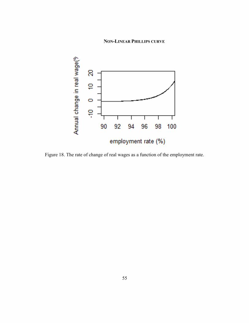
55

NON-LINEAR PHILLIPS CURVE

Figure 18. The rate of change of real wages as a function of the employment rate.

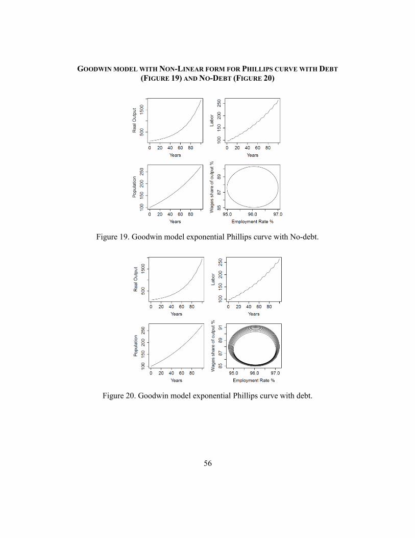
56

GOODWIN MODEL WITH NON-LINEAR FORM FOR PHILLIPS CURVE WITH DEBT

(FIGURE 19) AND NO-DEBT (FIGURE 20)

Figure 19. Goodwin model exponential Phillips curve with No-debt.

Figure 20. Goodwin model exponential Phillips curve with debt.

57

4. CHAPTER 4: RESEARCH DESIGN

4.1. SCOPE OF RESEARCH

The scope of the research will be to merge the models (Table 1) discussed so far

and while doing so maintain consistency in order to answer the research question in the

most effective way. The Biophysical model “HANDY” (Motesharrei, Rivas and Kalnay

2014) will be merged with the Goodwin model with Debt and No-Debt as described in

Keen, 2013. In the “HANDY” model everything eventually comes from nature, the

commoners extract nature which in return gets stored as accumulated wealth. This wealth

is then consumed by both the elites and the commoners. The economic model described by

Keen considers an exponential growth of labor productivity at a constant rate α (Eq 48)

and thus determining the output according to the Eq 22. It also considers an exponential

growth for population (Eq 49) unlike in “HANDY” where the population (Eq 35) is the

difference between the births and deaths and death rate being a function of total

accumulated wealth (Eq 39 & Eq 42).

Assumptions in the merged model:

1. There is only one kind of population as defined in “HANDY” (Eq 35) in our

merged model which will be categorized into 2 kinds:

a. Employed Labor (the part of the population that is employed), and

b. Unemployed Labor (the population that isn’t part of the labor that

contributes to the growth of the economy)

2. When the rate of extraction (depletion) of nature is assumed to need labor as an

input, the merged model explicitly considers only employed peoples as labor,

whereas in HANDY the entire commoner population, with no concept of

58

employment is assumed as working to extract the nature in order to accumulate

wealth.

3. Labor is defined in our model under the assumption of full utilization of capital

in the Leontief production function and can be calculated from the equation 𝑌 =

𝑎𝐿 = 𝐾/𝑣 similar as in Keen (2013).

4. A constant rate of interest is assumed on the debt accumulated towards

investment.

59

Table 1. Equations for the merged model

“HANDY” Equations (Motesharrei et.

al, 2014)

Keen, 2013 Equations

1. 𝑑

𝑑𝑡𝑥𝑐 = 𝛽𝑐𝑥𝑐 − 𝛼𝑐𝑥𝑐 ; Eq 35

2. 𝑑

𝑑𝑡𝑥𝑒 = 𝛽𝑒𝑥𝑒 − 𝛼𝑒𝑥𝑒 ; Eq 36

3. 𝑑

𝑑𝑡𝑦 = 𝛾 𝑦 (𝜆 − 𝑦 ) − 𝛿𝑥𝑐𝑦 ; Eq

37

4. 𝑑

𝑑𝑡𝑤 = 𝛿 𝑥𝑐𝑦 − 𝐶𝑐 − 𝐶𝑒 ; Eq 38

1. 𝑑𝑌

𝑑𝑡= 𝑌(

𝐼(∏

𝑣𝑌)

𝑣−𝛾); Eq 45

2. 𝑑𝑤

𝑑𝑡= 𝑝ℎ(𝜆)𝑤; Eq 46

3. 𝑑𝐷

𝑑𝑡= 𝐼 (

∏

𝑣𝑌) Y- ∏ ; Eq 47

4. 𝑑𝑎

𝑑𝑡= 𝛼𝑎; Eq 48

5. 𝑑𝑁

𝑑𝑡= 𝛽𝑁; Eq 49

MERGED EQUATIONS

1. 𝑑𝑥ℎ𝑐

𝑑𝑡= 𝛽ℎ𝑐𝑥ℎ𝑐 − 𝛼ℎ𝑐𝑥ℎ𝑐; Eq 53

2. 𝑑𝑦ℎ

𝑑𝑡= 𝛾ℎ𝑦ℎ(𝜆ℎ − 𝑦ℎ ) − 𝛿𝐿𝑦ℎ; Eq 54

3. 𝑑𝑤ℎ

𝑑𝑡= 𝛿𝐿𝑦ℎ − 𝐶ℎ𝑐; Eq 55

4. 𝑑𝑌

𝑑𝑡= 𝑌 (

𝐼(∏

𝑣𝑌)

𝑣− 𝛾) ; Eq 56

5. 𝑑𝑤

𝑑𝑡= 𝑝ℎ (𝜆)𝑤; Eq 57

6. 𝑑𝑎

𝑑𝑡= 𝛼𝑎; Eq 58

7. 𝑑𝐷

𝑑𝑡= 𝐼 (

∏

𝑣𝑌) Y- ∏; Eq 59

60

Figure 21. The above diagram explains the how the 2 models have been

integrated to understand the dynamics of the merged model.

The concepts of Output (Y), Labor (L) and Debt (D) and exponential growth in

labor productivity (a) will be used to understand their feedback on biophysical parameters

like population and nature in “HANDY”. Thus, modifying the nature extraction (depletion)

function and the accumulated wealth in the Handy model to that as above (Eq 54 & Eq 55

respectively).

In this chapter, I introduce alternative functions to describe nature extraction

(depletion) function in the merged model to understand the implications of different

assumptions. The different types of nature extraction (depletion) function are:

a. Nature extraction (depletion) as a function of Labor (L)

𝑁𝑎𝑡𝑢𝑟𝑒 𝐸𝑥𝑡𝑟𝑎𝑐𝑡𝑖𝑜𝑛 = 𝛿𝐿𝐿𝑦ℎ Eq 60

61

b. Nature extraction (depletion) as a function of Capital (K)

𝑁𝑎𝑡𝑢𝑟𝑒 𝐸𝑥𝑡𝑟𝑎𝑐𝑡𝑖𝑜𝑛 = 𝛿𝐾𝐾𝑦ℎ Eq 61

c. Nature extraction (depletion) as a function of Power Input (Pi)

We define Power Input (Pi) as a portion of wealth denoted by 𝛿𝑃𝑖𝑤𝑒𝑎𝑙𝑡ℎ−1𝑡𝑖𝑚𝑒−1

towards providing power to extract nature and therefore,

𝑁𝑎𝑡𝑢𝑟𝑒 𝐸𝑥𝑡𝑟𝑎𝑐𝑡𝑖𝑜𝑛 = 𝛿𝑃𝑖𝑃𝑖𝑦ℎ Eq 62

d. Depreciation of Wealth

The concept of depreciation was missing for accumulated wealth in HANDY and

therefore we will have it in our model to understand its impact. Depreciation of wealth in

our model is represented by 𝛿ℎ which has a constant value of 1%/yr. and modifies the

wealth equations as below:

𝑑

𝑑𝑡𝑤ℎ = 𝛿𝐿𝐿𝑦ℎ − 𝐶ℎ𝑐 − 𝛿ℎ𝑤ℎ Eq 63

𝑑

𝑑𝑡𝑤ℎ = 𝛿𝐾𝐾𝑦ℎ − 𝐶ℎ𝑐 − 𝛿ℎ𝑤ℎ Eq 64

𝑑

𝑑𝑡𝑤ℎ = 𝛿𝑃𝑖𝑃𝑖𝑦ℎ − 𝐶ℎ𝑐 − 𝛿ℎ𝑤ℎ Eq 65

4.2. OVERVIEW OF METHODOLOGY

There are a couple of ways to merge the two models while either keeping the

parameters the same or altering them to help us understand the research question. Most of

the parameters in both the models have been kept the same except a few listed below in

Figure 22.The predominant idea is to try out different forms for the Nature Extraction

(depletion) function but there are other parameters that affect the models and it’s important

to understand their feedbacks to use the best approach

62

Figure 22. Different parameters from both the models which will be tweaked in the merged

model to understand how sensitive the model is to these parameters.

4.3. RESEARCH GOAL

The research goal of the study here would be to identify the best scenario after

simulating the different scenarios discussed above in section 4.2. and try to understand it

in detail and confirm if the results are consistent with the other two models.

63

5. CHAPTER 5: RESULTS AND FINDINGS

5.1. NATURE EXTRACTION AS A FUNCTION OF LABOR

In this section, we assume that only labor (L) is used to extract nature which gets

stored as wealth and is consumed by the total population in the system (both the employed

and the unemployed population in the model).

5.1.1. NATURE EXTRACTION AS A FUNCTION OF LABOR NOT INCLUDING DEBT AND A

LINEAR FORM FOR THE PHILLIPS CURVE

I model the merged equations from the 2 models (“HANDY” + “Goodwin + Debt”)

as in Table 1 without debt, and using a linear form for the Phillips curve equation 𝑝ℎ(𝜆) =

−𝐶 + 𝑑𝜆 as seen in Eq 26. Figure 23 shows the results of simulating the equations with a

baseline extraction rate 𝛿𝐿,𝑜 = 6.67×10−6. After simulating the model for 500 years the

accumulated wealth, available nature, and population reaching a steady state between 300

to 400 years. The output grows continuously through the entire period with declining

profits. The profit rate remains positive during the entire simulation. The profit rate (Keen,

1995, 616) in the model fluctuates in the range of 0.03 to 0.08 for ~ 200 years and declines

as wage share increases.

Without Debt,

𝑃𝑟𝑜𝑓𝑖𝑡 𝑅𝑎𝑡𝑒 =1

𝑣(1 −

𝑤

𝑎) Eq 66

With Debt,

𝑃𝑟𝑜𝑓𝑖𝑡 𝑅𝑎𝑡𝑒 =1

𝑣(1 −

𝑤

𝑎−

𝑟𝐷

𝑌) Eq 67

64

Figure 44 shows results when the extraction rate is changed from 0.5 to 5 times the

baseline extraction rate 𝛿𝐿,𝑜. Higher extraction rates 𝛿𝐿 > 2.5 𝛿𝐿,𝑜 causes a more rapid

growth in population and output, but eventually nature is depleted (to very near zero) and

most wealth is consumed such that the population crashes after reaching its peak. Nature

doesn’t accumulate to a significant degree that total consumption is small enough for nature

to grow back. The higher the extraction rate, the further nature is depleted, the longer nature

takes to accumulate, and thus the closer population declines to zero.

65

Figure 23. Simulation result when extraction rate of nature is only a function of Labor,

and a baseline rate of extraction 𝛿𝐿,𝑜 = 6.67×10−6𝑝𝑒𝑟𝑠𝑜𝑛−1𝑡𝑖𝑚𝑒−1. Wages being

modeled according to a linear form of the Phillips curve without including debt.

66

5.1.2. NATURE EXTRACTION AS A FUNCTION OF LABOR INCLUDING DEBT, LINEAR

PHILLIPS CURVE, AND A NONLINEAR INVESTMENT CURVE

When Debt (Eq 47) is introduced in the above model with a constant rate of interest

of 5% its simulation results can be seen in Figure 24. Unlike in the previous case that does

not include debt, the system states do not reach steady state. Thus, resulting in declining

population, output, and profit rate due to rising debt. The system blows up (~400 years) as

the debt keeps on accumulating rapidly and beyond which the simulations for wage share

and employment rate start going erratic. Figure 46 shows the effect of varying the

extraction rates, and similar observations can be made as in the previous case with no debt.

An earlier collapse occurs as the extraction rate increases. Figure 47 highlights the effect

of different values for constant rate of interests. As the constant rate of interest on debt

increases from 2% to 5% the system collapse occurs relatively earlier. However, for interest

rates < 2% the system avoids collapse within the simulated time of 500 years but when the

model is simulated for a longer period of time (Figure 45) a collapse occurs eventually due

to rising debt even at a lower interest rate.

67


with a baseline extraction rate 𝛿𝐿,𝑜 = 6.67×10−6 with debt being accumulated at a

constat rate of interest 𝑟 = 5% and a Linear form for the Phillips curve.

68

5.1.3. NATURE EXTRACTION AS A FUNCTION OF LABOR WITHOUT DEBT, NONLINEAR


The Keen, 2013 paper suggested that a nonlinear form for the Phillips curve (Eq

52) would better the rate of change of real wages, 𝑤. Figure 25 shows the results for

simulating the model with the nonlinear form for the Phillips curve with no debt in the

model. The model shows similar results to as in Figure 23 at an Extraction rate of 𝛿𝐿,𝑜 =

6.67×10−6. Figure 48 shows results when the extraction rate is varied from 0.5 to 5 times

𝛿𝐿,𝑜 where similar results can be interpreted that, increasing extraction rate leads to an

earlier collapse in the model, same as in the case with the linear form for the linear Phillips

curve.

69


with a baseline extraction rate 𝛿𝐿,𝑜 = 6.67×10−6 without debt and a nonlinear form for

the Phillips curve.

70

5.1.4. NATURE EXTRACTION AS A FUNCTION OF LABOR INCLUDING DEBT NONLINEAR


When debt is included in the model with a nonlinear form for the Phillips curve a

debt-induced collapse is observed (Figure 26) similar to that of when a linear Phillips curve

was used in the previous section 5.1.2. Similar results to that of Figure 46 and Figure 47

can be seen in Figure 49 and Figure 50 when the rate of extraction of nature and the constant

rate of interest on the debt is varied. System collapse occur earlier when increasing value

of 𝛿𝐿,𝑜 and 𝑟. Charging higher rates of interest on debt increases debt payments and leads

to earlier collapse.

71


with a baseline extraction rate 𝛿𝐿,𝑜 = 6.67×10−6 .Where debt is being accumulated at

a constat rate of interest of (𝑟) 5% and and wages modeled according to a noninear

form of the Phillips curve.

72

5.2. NATURE EXTRACTION AS A FUNCTION OF CAPITAL

In the previous section 5.1, we had modeled the rate of extraction of nature as a

function of only labor. In this section, we will model the rate of extraction of nature as a

function of only capital (Eq 61). The assumption here is that the machines only (or the

money needed to purchase machines) are needed to extract nature, but neither labor or

wealth are explicitly needed for nature extraction. The purpose of this assumption is to

explore the influence on simulation results from nature extraction being a function of

capital. The baseline rate of extraction of nature is specified as 𝛿𝐾,𝑜 = 3.335×

10−7𝑐𝑎𝑝𝑖𝑡𝑎𝑙−1𝑡𝑖𝑚𝑒−1. One very important thing to consider while going through the

results in this section is that, when either the wage share or the employment rate go beyond

realistic values i.e. wage share > 100% or employment rate > 100% the model behaves

erratically and the results beyond that point become inconceivable and therefore should be

ignored.

5.2.1. NATURE EXTRACTION AS A FUNCTION OF CAPITAL WITHOUT DEBT AND A LINEAR

FORM OF THE PHILLIPS CURVE

Here we model the set of equations in Table 1 with the difference that the nature

extraction is a function of only capital (Eq 61). Figure 27 shows the results of the simulation

at 𝛿𝐾,𝑜 = 3.335×10−7𝑐𝑎𝑝𝑖𝑡𝑎𝑙−1𝑡𝑖𝑚𝑒−1 and no debt. The observations can be

summarized as below:

All nature gets exhausted around 220 years without regenerating for rest of the

simulation. Once nature gets exhausted the population sustains for further longer time

based on the accumulated wealth during the years before nature is exhausted. Once the

accumulated wealth starts declining a fall in the population and output is observed. The

decline in output can be explained by a decline in labor which is itself driven by a decline

73

in population.30Figure 51 shows results when the rate of extraction of nature as a function

of capital is varied from 0.5 to 5 times the baseline value 𝛿𝐾,𝑜 = 3.335×

10−7𝑐𝑎𝑝𝑖𝑡𝑎𝑙−1𝑡𝑖𝑚𝑒−1. The major conclusion from simulating nature extraction as a

function of capital is that this assumption always causes the full depletion of nature,

eventually resulting in a collapse. The higher the value of 𝛿𝐾, the earlier the collapse is

observed in the system. Also, the profit rate here goes negative with increasing wage share

according to Eq 66. As the population decreases the wage share increases, the reasoning

behind this could be that the firms try to employ people by paying them higher wages until

the population totally collapses.

30 𝑂𝑢𝑡𝑝𝑢𝑡 (𝑌) = 𝑎(𝐿𝑎𝑏𝑜𝑟 𝑃𝑟𝑜𝑑𝑢𝑐𝑡𝑖𝑣𝑖𝑡𝑦) ∗ 𝐿(𝐿𝑎𝑏𝑜𝑟)

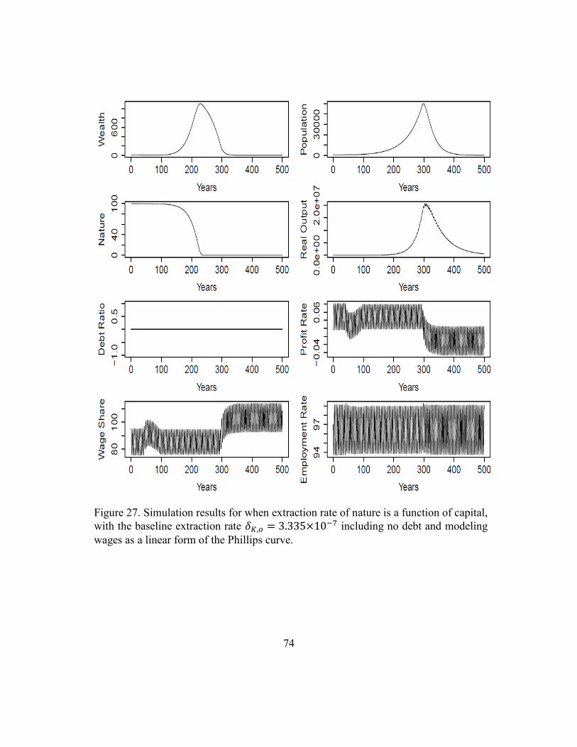
74

Figure 27. Simulation results for when extraction rate of nature is a function of capital,

with the baseline extraction rate 𝛿𝐾,𝑜 = 3.335×10−7 including no debt and modeling

wages as a linear form of the Phillips curve.

75

5.2.2. NATURE EXTRACTION AS A FUNCTION OF CAPITAL INCLUDING DEBT AND A

LINEAR FORM OF THE PHILLIPS CURVE

Figure 28 describes the scenario when debt is included in the model. By including

debt at 5% interest, the simulation no longer indicates the full depletion of nature under the

baseline extraction rate. As the accumulated debt rises, debt payments also increase which

then decreases profits. Decreasing profit results in decreasing output and with decreasing

output the capital going towards nature extraction declines as well (Eq 23).

Figure 52 shows the effect of increasing 𝛿𝐾,𝑜 in the model. Larger values of 𝛿𝐾

cause earlier collapse in the system. Figure 53 shows the effect of changing constant rate

of interest. At lower values of interest rates, full extraction of nature occurs whereas, at a

higher rate of interest the extraction of nature occurs slowly. This gives time for the

population to grow and once the debt levels start to rise, the profit rate (Eq 67) starts to fall

thus resulting in declining output. With declining output, the capital towards extraction of

nature declines as well (Eq 23). Therefore, nature starts to regenerate and the population

starts declining as not enough wealth is being accumulated to be consumed by the

population.

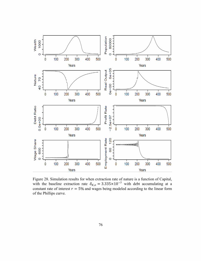
76


with the baseline extraction rate 𝛿𝐾,𝑜 = 3.335×10−7 with debt accumulating at a

constant rate of interest 𝑟 = 5% and wages being modeled according to the linear form

of the Phillips curve.

77

5.2.3. NATURE EXTRACTION AS A FUNCTION OF CAPITAL WITHOUT DEBT AND A

NONLINEAR FORM OF THE PHILLIPS CURVE

In this section, we will look at the simulation results when the wages are modeled

according to the nonlinear form for the Phillips curve (Eq 52) and nature is a function of

capital as in the previous section. Figure 29 shows results of the basic simulation with

𝛿𝐾,𝑜 = 3.335×10−7 and the nonlinear form for the Phillips curve. The results look similar

to the results in the Figure 27, where all the nature is extracted towards accumulating wealth

and not regenerating once gone because the rate of extraction is greater than the rate of

regeneration under the given set of parameters. On increasing the 𝛿𝐾 value (Figure 54)

similar results as observed earlier in Figure 51 can be observed where increasing 𝛿𝐾 causes

an earlier collapse in the system.

78


with the baseline extraction rate 𝛿𝐾,𝑜 = 3.335×10−7 with no debt accumulating and

the nonlinear form of the Phillips curve.

79

5.2.4. NATURE EXTRACTION AS A FUNCTION OF CAPITAL INCLUDING DEBT, NONLINEAR

FORM OF THE PHILLIPS CURVE, AND A NONLINEAR FORM OF THE INVESTMENT CURVE

In this section, we will discuss the results when simulating nature as a function of

capital (Eq 61) including debt and a nonlinear form for the Phillips curve equation (Eq 52).

Total Nature is still extracted in the model (Figure 30) when debt is included. The debt

blows up when the wealth is totally exhausted leading to a collapse in the population after

which the simulation does not provide any conceivable results (~300 years). When the 𝛿𝐾

is increased similar behavior as in earlier simulations is observed where the collapse occurs

earlier (Figure 55). Figure 56 shows the results for the effect the constant rate of interest 𝑟

has on the model where it is a function of only capital. Here a debt induced collapse doesn’t

happen like in Figure 53 where we had the linear form for the Phillips curve but when we

increase the value of 𝑟 to 7% a similar collapse is observed to happen (Figure 31). The

reason is that the accumulated debt when assuming a debt @5% constant rate of interest

(under the given set of parameters) with the nonlinear form for the Phillips curve isn’t

enough to induce collapse due to debt accumulation but however a collapse is induced by

depletion of nature. Even at lower interest rates the, system keeps extracting the nature

until fully exhausted.

In brief, while modeling nature extraction as a function of capital, if interest rates

are high enough, a debt-induced collapse occurs before nature is depleted. At low enough

interest rates, collapse occurs due to depletion of nature before too much debt is

accumulated. However, under no tested conditions (different interest rates or rates of

extraction) can a non-zero steady state population simulated.

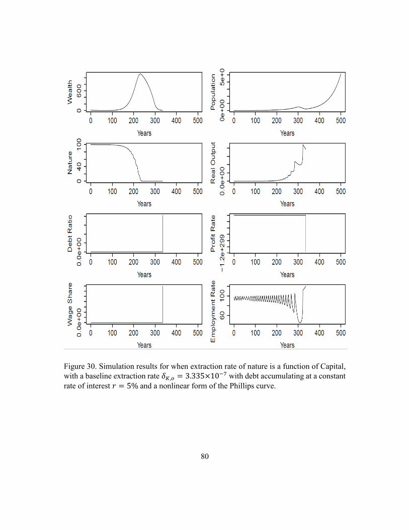
80


with a baseline extraction rate 𝛿𝐾,𝑜 = 3.335×10−7 with debt accumulating at a constant

rate of interest 𝑟 = 5% and a nonlinear form of the Phillips curve.

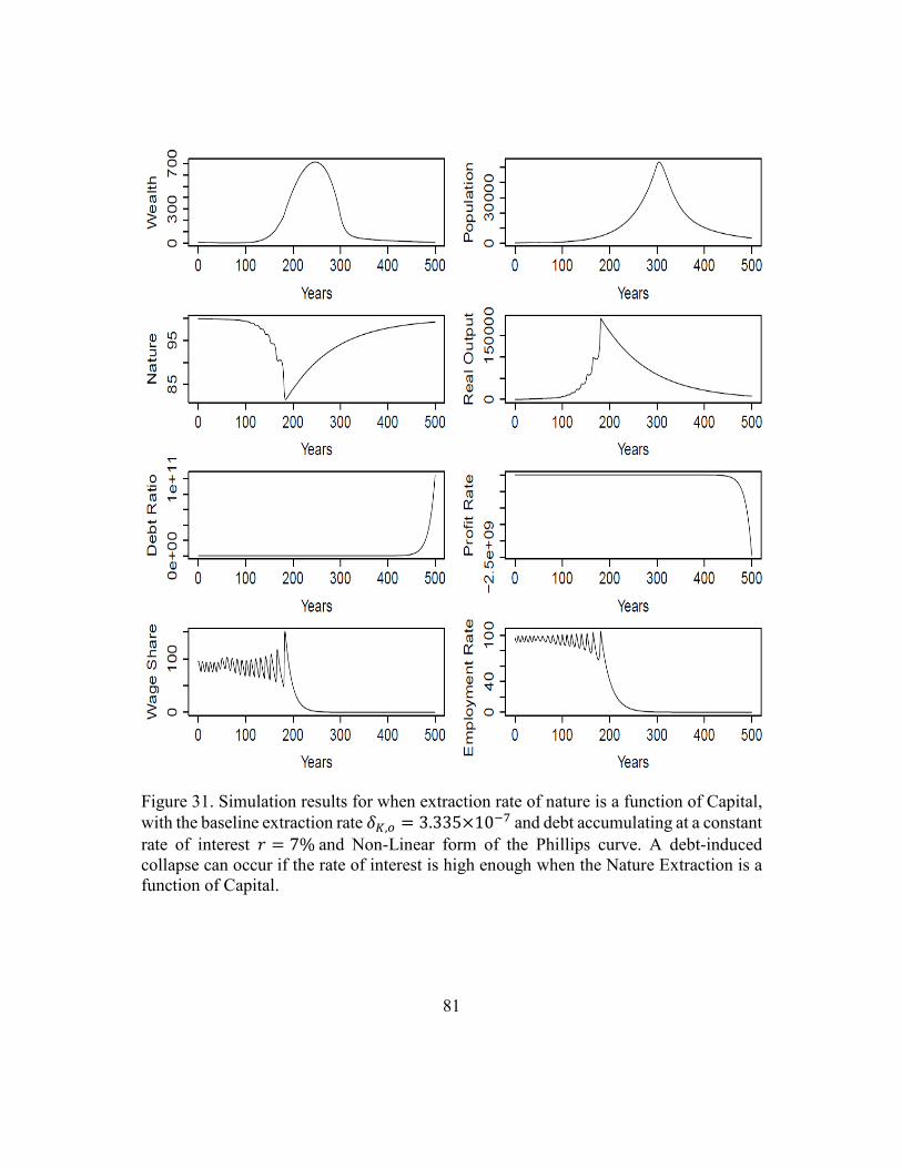
81


with the baseline extraction rate 𝛿𝐾,𝑜 = 3.335×10−7 and debt accumulating at a constant

rate of interest 𝑟 = 7% and Non-Linear form of the Phillips curve. A debt-induced

collapse can occur if the rate of interest is high enough when the Nature Extraction is a

function of Capital.

82

5.3. NATURE EXTRACTION AS A FUNCTION OF POWER INPUT

In section 5.1 and section 5.2 we considered nature extraction as a function of only

labor and capital respectively. In this section, we will take a look at the results when the

nature extraction is a function of power input. We define power input 𝑃𝑖 (Eq 68) as the

power required to extract nature which will be extracted from the stored wealth and will

therefore be a function of the same. Also, in this section we will only consider wages

modeled as a nonlinear function of the Phillips curve as its effect on the model has been

demonstrated in the previous sections.

5.3.1. NATURE AS A FUNCTION OF POWER INPUT WITH A NONLINEAR FORM OF THE

PHILLIPS CURVE WITHOUT DEBT

Here we would experiment with a new parameter defined as power input. The

concept here is that the wealth stored (e.g., nature that is extracted but not yet consumed)

in HANDY which initially was used only for the consumption by the population. In this

section, I create an additional consumption of wealth that is the power input. The power

input is defined as a fraction of accumulated wealth that is used to extract the nature. Thus,

the rate of extraction of nature is now a function of how much wealth has been accumulated

(Eq 62).

𝑃𝑜𝑤𝑒𝑟 𝐼𝑛𝑝𝑢𝑡 = 𝑝𝑓×𝑤ℎ Eq 68

Where, pf is the power factor and equal to 1%/𝑦𝑒𝑎𝑟 × 𝑤ℎ.The baseline depletion

factor, in this case, is defined as 𝛿𝑃𝑖,𝑜 and equal to 0.3335 (𝑝𝑜𝑤𝑒𝑟 𝑖𝑛𝑝𝑢𝑡)−1𝑡𝑖𝑚𝑒−1.

Simulation results with nature extraction a function of power input can be seen in Figure

32 where nature is extracted very rapidly at the beginning but eventually reaches a steady

83

state. The population rises at the beginning with extraction of nature but reaches a steady

state at approximately the same time as nature (~200 years). Whereas, output keeps

continuously growing exhibiting a scenario where exponential growth is possible in a

system while attaining a sustainable population.

When 𝛿𝑃𝑖 is varied from 0.5 to 5 times its baseline extraction rate 𝛿𝑃𝑖,𝑜 (Figure

57) its baseline value, higher population peaks are attained at lower 𝛿𝑃𝑖 values in

comparison to higher values for 𝛿𝑃𝑖. However, reaching steady state in all cases. Whereas,

output grows exponentially for different values of 𝛿𝑃𝑖 similar as in Figure 32 at a slower

rate for higher values of 𝛿𝑃𝑖.

The important result for these simulations that assume nature extraction is a

function of power input (e.g., wealth consumption) is that at a low enough depletion factor,

𝛿𝑃𝑖, the population and available nature can reach a steady state. At a high enough depletion

factor such as 5𝛿𝑃𝑖,𝑜, the population oscillates about a relatively low level.

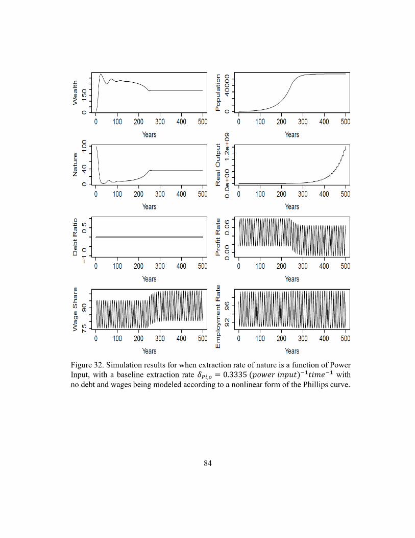
84


Input, with a baseline extraction rate 𝛿𝑃𝑖,𝑜 = 0.3335 (𝑝𝑜𝑤𝑒𝑟 𝑖𝑛𝑝𝑢𝑡)−1𝑡𝑖𝑚𝑒−1 with

no debt and wages being modeled according to a nonlinear form of the Phillips curve.

85

5.3.2. NATURE AS A FUNCTION OF POWER INPUT IN THE MODEL WITH A NONLINEAR

FORM OF THE PHILLIPS CURVE INCLUDING DEBT

When debt is included in the model with nature extraction a function of power

input, similar results can be observed in Figure 33 and Figure 58 to that as in the previous

section with the difference of declining output and profit rate. In Figure 33, near the end of

the simulation period, debt begins to increase rapidly as the population growth slows. By

increasing the depletion factor 𝛿𝑃𝑖, the exponential debt accumulation begins earlier as

nature becomes fully depleted.

Figure 59 highlights that there is no effect in either the population, available nature,

or the output when the constant rate of interest on the debt is varied in the model. This is

because there is no feedback from the economic model (Goodwin with Debt, Keen, 2013)

to the parameters in the biophysical model (“HANDY’). In previous sections (5.1 and 5.2)

nature extraction was a function of Labor and Capital, both these parameters were from the

economic model and therefore affected the parameters in the biophysical model. Whereas

here the nature extraction is a function of power input which is a function of wealth from

the biophysical model. Therefore, no feedbacks are observed in the population, available

nature etc.

86


Input, with the baseline extraction rate 𝛿𝑃𝑖,𝑜 = 0.3335 (𝑝𝑜𝑤𝑒𝑟 𝑖𝑛𝑝𝑢𝑡)−1𝑡𝑖𝑚𝑒−1 with

debt accumulating at r=5% and wages modeled according to the nonlinear form of the

Phillips curve.

87

5.3.3. VARYING POWER FACTOR FROM 1% OF WEALTH TO 20% OF WEALTH BEING

USED AS POWER INPUT TOWARDS EXTRACTING NATURE

In this section, the power factor pf is varied from 1%/yr. of wealth to 20%/yr. of

wealth in order to understand its effect on the system. Figure 34 shows results when the

power factor (pf) is increased from 1% to 20%. Higher values of pf result in lower peaks

of the population and higher oscillations in available nature. The system seems to be

reaching a steady state in all cases with higher output at lower values of pf. An interesting

thing to observe is that the amount of debt accumulated is higher at higher values of pf.

Implying, that the level of debt rises with decreasing population as there is less wealth to

be consumed by the population and thus leading to no debt payments in the system.

88

Figure 34. Simulating results by altering the power factor pf from 1% to 20% of wealth

for when nature extraction is a function of Power Input, with the baseline extraction rate

𝛿𝑃𝑖,𝑜 = 0.3335 (𝑝𝑜𝑤𝑒𝑟 𝑖𝑛𝑝𝑢𝑡)−1𝑡𝑖𝑚𝑒−1 including debt and wages modeled as a

nonlinear form of the Phillips curve.

5.4. INCLUDING DEPRECIATION OF WEALTH

In the earlier sections, we didn’t consider any kind of depreciation in the

biophysical model “HANDY”. The capital depreciates at a constant rate of 𝛾 in

determining the rate of change of capital 𝐾. Therefore, in this section introduce

depreciation of accumulated wealth in all the 3 scenarios discussed above where

1. Accumulated wealth when nature extraction is a function of Labor Eq 63

2. Accumulated wealth when nature extraction is a function of Capital Eq 64

89

and,

3. Accumulated wealth when nature extraction is a function of Power Input Eq 65

Figure 35 through Figure 37 show simulated results while assuming the

depreciation of wealth 𝛿ℎ = 1%/𝑦𝑟. When compared to results with no wealth

depreciation the population and wealth peaks are lower with depreciation, the population

and wealth peaks are lower with depreciation. This difference is intuitive because as wealth

depreciates before it can be consumed by the population, the population consume less

wealth and is not able to grow as high of a peak population.

90

5.4.1. COMPARING RESULTS WITH AND WITHOUT DEPRECIATION OF WEALTH WHEN

NATURE EXTRACTION IS A FUNCTION OF LABOR.

Figure 35. Simulating results for when nature is a function of labor with and without



baseline extraction rate 𝛿𝐿,𝑜 = 6.67×10−6𝑝𝑒𝑟𝑠𝑜𝑛−1𝑡𝑖𝑚𝑒−1 is same as in section 5.1.

91


NATURE EXTRACTION IS A FUNCTION OF CAPITAL

Figure 36. Simulating results for when nature is a function of capital with and without



baseline extraction rate 𝛿𝐾,𝑜 = 3.335×10−7𝑐𝑎𝑝𝑖𝑡𝑎𝑙−1𝑡𝑖𝑚𝑒−1 is same as in section 5.2.

92


NATURE EXTRACTION IS A FUNCTION OF POWER INPUT

Figure 37. Simulating results for when nature is a function of power input with and

without depreciation of wealth in the model. Here a nonlinear form of the Phillips curve

is considered to model wages with a nonlinear form for investment including debt. The

baseline extraction rate 𝛿𝑃𝑖,𝑜 = 0.3335 (𝑝𝑜𝑤𝑒𝑟 𝑖𝑛𝑝𝑢𝑡)−1𝑡𝑖𝑚𝑒−1 is same as in section

5.3.

93

6. CHAPTER 6: DISCUSSIONS

6.1. OVERVIEW

In the previous sections, we have seen different scenarios for when nature

extraction is a function of labor, capital, power input and the impact debt has in each case.

In this section, I perform additional sensitivity in the model by increasing the constant rate

of interest on debt from 5% to 15%. I will also compare the results with when there is no

debt in the model and clearly highlight how critical the role of debt is.

6.1.1. EFFECT OF DEBT AT HIGH CONSTANT RATE OF INTERESTS WHEN NATURE

EXTRACTION IS A FUNCTION OF LABOR

When we increase the rate of interest on debt from 5 to 15% the population begins

to decline sooner at a higher value of interest rates (Figure 39). Declining population also

results in an early regeneration of nature and therefore results in it returning back to its

original value (Figure 38). However, the population and nature both seem to reach a steady

state without debt in the system, clearly highlighting that a debt-induced collapse has

occurred in the model.

94

Figure 38. Simulating nature as a function of labor including debt for interest rates 5%

to 15% and no debt at a rate of extraction of nature 𝛿𝐿,𝑜 = 6.67×10−6𝑝𝑒𝑟𝑠𝑜𝑛−1𝑡𝑖𝑚𝑒−1.

Higher interest rates lead to an earlier collapse of nature while reaching a steady state

without debt.

95

Figure 39.Simulating nature as a function of labor including debt for interest rates 5% to

15% and no debt at a rate of extraction of nature 𝛿𝐿,𝑜 = 6.67×10−6𝑝𝑒𝑟𝑠𝑜𝑛−1𝑡𝑖𝑚𝑒−1.

Higher interest rates lead to an earlier collapse of population while reaching a steady

state without debt.


EXTRACTION IS A FUNCTION OF CAPITAL

In the case of assuming nature extraction is only a function of capital, when we

increase the rate of interest on debt from 5 to 15%, the population declines sooner at high-

interest rates (Figure 41), similar to that in the previous section 6.1.1. The difference here

is that nature doesn’t regenerate at low-interest rates and neither reaches a steady state

when there is no debt in the model (Figure 40). The reasoning behind which has been

discussed earlier in the sections 5.2.3 and 5.2.4.

96


to 15% and no debt at a rate of extraction of nature 𝛿𝐾,𝑜 = 3.335×10−7𝑐𝑎𝑝𝑖𝑡𝑎𝑙−1𝑡𝑖𝑚𝑒−1. Higher interest rates lead to an earlier collapse of nature whereas

the nature is fully extracted at low interest rates and no debt.

97


to 15% and no debt at a rate of extraction of nature 𝛿𝐾,𝑜 = 3.335×10−7𝑐𝑎𝑝𝑖𝑡𝑎𝑙−1𝑡𝑖𝑚𝑒−1. Higher interest rates lead to an earlier collapse of population.


EXTRACTION IS A FUNCTION OF POWER INPUT

In this section, we will discuss the impact of the high constant rate of interests on

debt when nature extraction is a function of power input. When the constant rate of interest

r on debt is increased from 5 to 15%, no effect is observed in the population (Figure 43) and

similarly in the available nature (Figure 42). A very similar behavior was also observed

when the rate of interest on the debt was varied from 1 to 5% (Figure 59). The reasoning

behind which has been discussed in section 5.3.2.

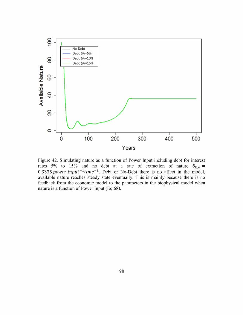
98

Figure 42. Simulating nature as a function of Power Input including debt for interest

rates 5% to 15% and no debt at a rate of extraction of nature 𝛿𝐾,𝑜 =0.3335 𝑝𝑜𝑤𝑒𝑟 𝑖𝑛𝑝𝑢𝑡−1𝑡𝑖𝑚𝑒−1. Debt or No-Debt there is no affect in the model,

available nature reaches steady state eventually. This is mainly because there is no

feedback from the economic model to the parameters in the biophysical model when

nature is a function of Power Input (Eq 68).

99

Figure 43. Simulating nature as a function of Power Input including debt for interest

rates 5% to 15% and no debt at a rate of extraction of nature 𝛿𝐾,𝑜 =0.3335 𝑝𝑜𝑤𝑒𝑟 𝑖𝑛𝑝𝑢𝑡−1𝑡𝑖𝑚𝑒−1. Debt or No-Debt there is no affect in the model, the

population reaches a steady state eventually. This is mainly because there is no feedback

from the economic model to the parameters in the biophysical model when nature is a

function of Power Input (Eq 68).

6.2. CONCLUSIONS

Debt has a direct impact in the merged biophysical and economic model when

nature extraction is either a function of labor (section 5.1) or capital (section 5.2) but no

impact when it’s a function of power input (section 5.3). The model is also sensitive to

other parameters like the constant rate of interest on debt, the linear and the nonlinear form

of the Phillips curve and the rate of extraction of nature. There is a positive correlation

between the constant rate of interest on debt and the speed of collapse occurring in the

100

model. Higher values for interest rates lead to an earlier collapse of the model. There is

also a correlation with the rate of extraction of nature where a collapse happens earlier at

higher values and gets delayed at lower values.

I investigated the effect of assuming either a linear or a nonlinear form for the

Phillips curve to model wages. It is important to notice that both seem to simulate very

similar results (Figure 23 to Figure 26) with one possible exception: when we model nature

as a function of capital including debt with the nonlinear form of the Phillips curve (section

5.2.4). The model no longer simulates realistic outcomes breaks ~330 years (Figure 30)

(i.e. when wealth reaches zero but population explodes beyond which the results don’t

make any conceivable sense).

Another interesting observation (for the case when nature extraction is a function

of capital including debt and the nonlinear form for the Phillips curve) is that for a given

set of model parameters, there is a threshold interest rate above which nature cannot be

fully depleted before a debt-induced collapse. For example, at 5% constant interest rate

(Figure 30), nature is fully depleted before debt prevents profitability, but there is a debt-

induced collapse at a higher constant interest rate of 7% (Figure 31) where employment

and profits go to zero but nature is not fully depleted.

A much deeper analysis is required before I can conclude which form of the Phillips

curve is best tailored for the model described in this thesis. suits the best to understand the

different dynamics happening in the model.

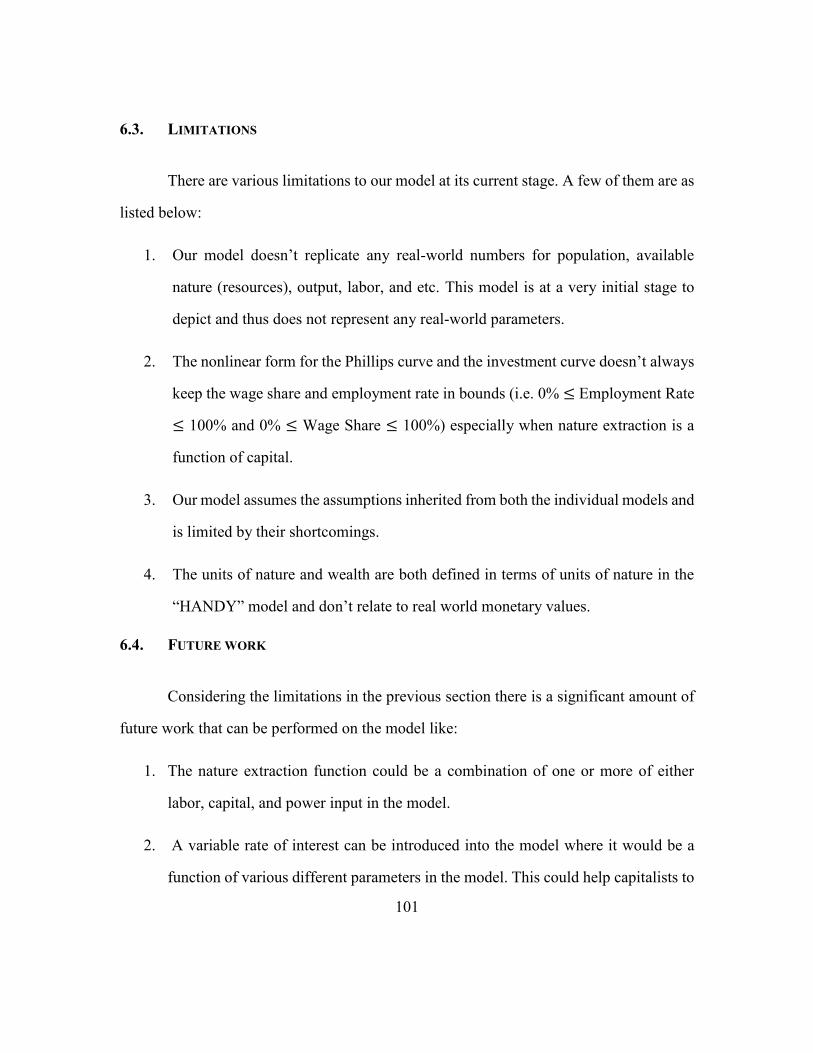
101

6.3. LIMITATIONS

There are various limitations to our model at its current stage. A few of them are as

listed below:

1. Our model doesn’t replicate any real-world numbers for population, available

nature (resources), output, labor, and etc. This model is at a very initial stage to

depict and thus does not represent any real-world parameters.

2. The nonlinear form for the Phillips curve and the investment curve doesn’t always

keep the wage share and employment rate in bounds (i.e. 0% ≤ Employment Rate

≤ 100% and 0% ≤ Wage Share ≤ 100%) especially when nature extraction is a

function of capital.

3. Our model assumes the assumptions inherited from both the individual models and

is limited by their shortcomings.

4. The units of nature and wealth are both defined in terms of units of nature in the

“HANDY” model and don’t relate to real world monetary values.

6.4. FUTURE WORK

Considering the limitations in the previous section there is a significant amount of

future work that can be performed on the model like:

1. The nature extraction function could be a combination of one or more of either

labor, capital, and power input in the model.

2. A variable rate of interest can be introduced into the model where it would be a

function of various different parameters in the model. This could help capitalists to

102

target a certain profit share by adjusting the different parameters that affect the

interest rate in the model.

3. A bank/ financial system like that of a Godley table (Godley and Lavoie 2006) can

be introduced to keep track of monetary flows in the model according to various

accounting rules.

4. Debt can be further classified into different types like household debt, government

debt, etc.

5. Age demographics can be included in the model to further classify the type of

population that exists in the model.

103

7. APPENDIX A-FIGURES & TABLES

Figure 44. Simulation results for when extraction rate of Nature is a function of Labor, with

a baseline extraction rate 𝛿𝐿,𝑜 = 6.67×10−6 being varied from 0.5𝛿𝐿,𝑜 𝑡𝑜 5𝛿𝐿,𝑜 without

debt and wages being modeled according to a Linear form of the Phillips curve.

104

Figure 45. Simulation results for 1000 years when extraction rate of nature is a function of

Labor, with the baseline extraction rate 𝛿𝐿,𝑜 = 6.67×10−6𝑝𝑒𝑟𝑠𝑜𝑛−1𝑡𝑖𝑚𝑒−1 a linear

Phillips curve, and debt accumulating at a constant interest rate of 1%/yr.

105

Figure 46. Simulation results for when extraction rate of Nature is a function of Labor, with

a baseline extraction rate 𝛿𝐿,𝑜 = 6.67×10−6 being varied from 0.5𝛿𝐿,𝑜 𝑡𝑜 5𝛿𝐿,𝑜 with debt

accumulating at a constat rate of interest of 𝑟 = 5% and wages being modeled according

to a linear form of the Phillips curve.

106

Figure 47. Simulation results for when extraction rate of nature is a function of Labor, with

a baseline extraction rate 𝛿𝐿,𝑜 = 6.67×10−6. While a constant rate of interest 𝑟 on Debt is

being varied from 1% 𝑡𝑜 5% with wages modeled according to the Linear form of Phillips

curve.

107


with the baseline extraction rate 𝛿𝐿,𝑜 = 6.67×10−6 being varied from 0.5𝛿𝐿,𝑜 𝑡𝑜 5𝛿𝐿,𝑜

and wages being modeled according to a noninear form of the Phillips curve.

108


a baseline extraction rate 𝛿𝐿,𝑜 = 6.67×10−6 being varied from 0.5𝛿𝐿,𝑜 𝑡𝑜 5𝛿𝐿,𝑜 with debt

accumulating at a constat interest rate, 𝑟 = 5% and wages modeled according to a

nonlinear form of the Phillips curve.

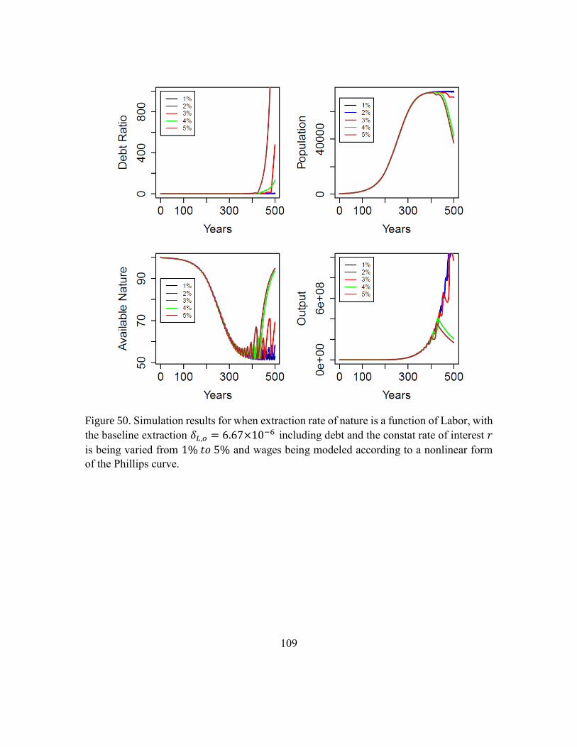
109


the baseline extraction 𝛿𝐿,𝑜 = 6.67×10−6 including debt and the constat rate of interest 𝑟

is being varied from 1% 𝑡𝑜 5% and wages being modeled according to a nonlinear form

of the Phillips curve.

110


with the baseline extraction rate 𝛿𝐾,𝑜 = 3.335×10−7 being varied from 0.5𝛿𝐾,𝑜 𝑡𝑜 5𝛿𝐾,𝑜

without debt and using a linear form of the Phillips curve to model wages.

111



including debt and a linear form of the Phillips curve to model wages.

112


with the baseline extraction rate 𝛿𝐾,𝑜 = 3.335×10−7including debt and the constant rate

of interest, 𝑟 is varied from 1% 𝑡𝑜 5% using a linear form of the Phillips curve to model

wages.

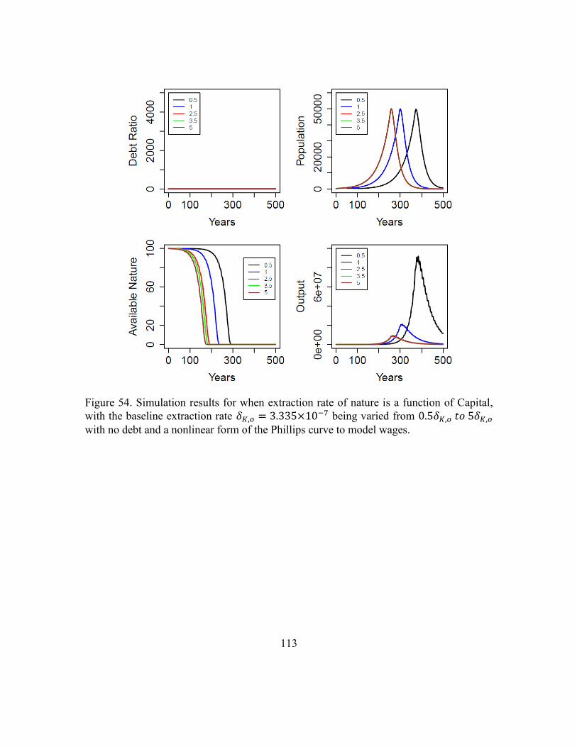
113



with no debt and a nonlinear form of the Phillips curve to model wages.

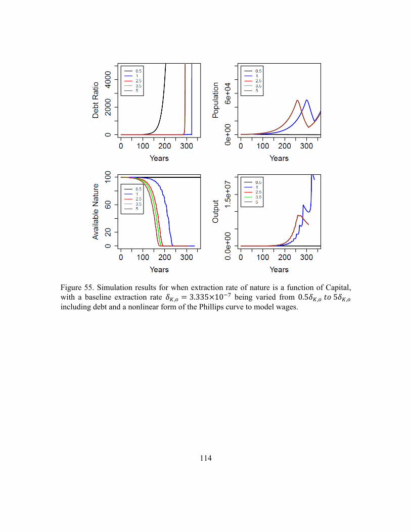
114


with a baseline extraction rate 𝛿𝐾,𝑜 = 3.335×10−7 being varied from 0.5𝛿𝐾,𝑜 𝑡𝑜 5𝛿𝐾,𝑜

including debt and a nonlinear form of the Phillips curve to model wages.

115


with the baseline extraction rate 𝛿𝐾,𝑜 = 3.335×10−7 including debt and the constant rate

of interest 𝑟 is being varied from 1% 𝑡𝑜 5% using a nonlinear form of the Phillips curve

to model wages.

116


Input, with the baseline extraction rate 𝛿𝑃𝑖,𝑜 = 0.3335 (𝑝𝑜𝑤𝑒𝑟 𝑖𝑛𝑝𝑢𝑡)−1𝑡𝑖𝑚𝑒−1 being

varied from 0.5𝛿𝑃𝑖,𝑜 𝑡𝑜 5𝛿𝑃𝑖,𝑜 without debt and a nonlinear form of the Phillips curve to

model wages.

117


Input, with the baseline extraction rate 𝛿𝑃𝑖,𝑜 = 0.3335 being varied from 0.5𝛿𝑃𝑖,𝑜 𝑡𝑜 5𝛿𝑃𝑖,𝑜

with debt being accumulated at a constant rate of interest, 𝑟 = 5% and a nonlinear form

of the Phillips curve to model wages.

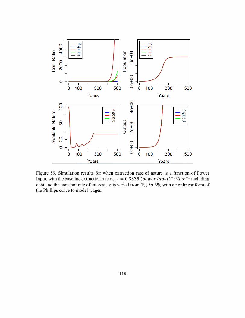
118


Input, with the baseline extraction rate 𝛿𝑃𝑖,𝑜 = 0.3335 (𝑝𝑜𝑤𝑒𝑟 𝑖𝑛𝑝𝑢𝑡)−1𝑡𝑖𝑚𝑒−1 including

debt and the constant rate of interest, 𝑟 is varied from 1% 𝑡𝑜 5% with a nonlinear form of

the Phillips curve to model wages.

119

Table 2. DIFFERENT PARAMETERS AND VARIABLES WITH THEIR VALUES USED TO

SIMULATE THE GOODWIN MODEL WITH OR WITHOUT DEBT, INCLUDING EITHER A LINEAR

OR A NONLINEAR FORM FOR THE PHILLIPS AND THE INVESTMENT CURVE AS IN KEEN,

2013.

Parameter Name Parameter

Symbol

Parameter

units

Initial Values in the

Model

Population 𝑁 people 100

Labor 𝐿 people 97

Labor productivity 𝑎 $/people 1

Output 𝑌 $ 97

Capital 𝐾 $ 291

Debt 𝐷 $ 0

Real Wage 𝑤 $/people 0.88

Rate of Growth of Labor

Productivity

𝛼 $/people/time 0.02

Constant Rate of Interest 𝑟 %/year 5

Depreciation of Capital 𝛾 /year 0.01

Capital to output ratio 𝑣 - 3

Parameters for Linear Phillips curve

Variable Description Value

𝑐 Constant in the Linear

Phillips curve

4.8

𝑑 Constant in the Linear

Phillips curve

5

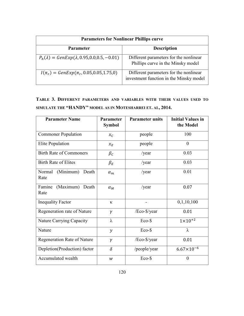
120

Parameters for Nonlinear Phillips curve

Parameter Description

𝑃ℎ(𝜆) = 𝐺𝑒𝑛𝐸𝑥𝑝(𝜆, 0.95,0.0,0.5, −0.01) Different parameters for the nonlinear

Phillips curve in the Minsky model

𝐼(𝜋𝑟) = 𝐺𝑒𝑛𝐸𝑥𝑝(𝜋𝑟 , 0.05,0.05,1.75,0) Different parameters for the nonlinear

investment function in the Minsky model

TABLE 3. DIFFERENT PARAMETERS AND VARIABLES WITH THEIR VALUES USED TO

SIMULATE THE “HANDY” MODEL AS IN MOTESHARREI ET. AL, 2014.


Symbol

Parameter units Initial Values in

the Model

Commoner Population 𝑥𝐶 people 100

Elite Population 𝑥𝐸 people 0

Birth Rate of Commoners 𝛽𝐶 /year 0.03

Birth Rate of Elites 𝛽𝐸 /year 0.03

Normal (Minimum) Death

Rate

𝛼𝑚 /year 0.01

Famine (Maximum) Death

Rate

𝛼𝑀 /year 0.07

Inequality Factor κ - 0,1,10,100

Regeneration rate of Nature 𝛾 /Eco-$/year 0.01

Nature Carrying Capacity λ Eco-$ 1×10+2

Nature 𝑦 Eco-$ λ

Regeneration Rate of Nature 𝛾 /Eco-$/year 0.01

Depletion(Production) factor 𝛿 /people/year 6.67×10−6

Accumulated wealth 𝑤 Eco-$ 0

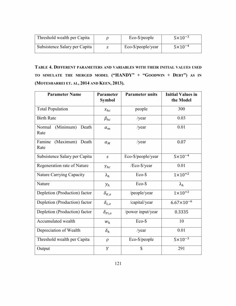
121

Threshold wealth per Capita ρ Eco-$/people 5×10−3

Subsistence Salary per Capita 𝑠 Eco-$/people/year 5×10−4

TABLE 4. DIFFERENT PARAMETERS AND VARIABLES WITH THEIR INITIAL VALUES USED

TO SIMULATE THE MERGED MODEL (“HANDY” + “GOODWIN + DEBT”) AS IN

(MOTESHARREI ET. AL, 2014 AND KEEN, 2013).


Symbol

Parameter units Initial Values in

the Model

Total Population 𝑥ℎ𝑐 people 300

Birth Rate 𝛽ℎ𝑐 /year 0.03

Normal (Minimum) Death

Rate

𝛼𝑚 /year 0.01

Famine (Maximum) Death

Rate

𝛼𝑀 /year 0.07

Subsistence Salary per Capita 𝑠 Eco-$/people/year 5×10−4

Regeneration rate of Nature 𝛾ℎ𝑐 /Eco-$/year 0.01

Nature Carrying Capacity λℎ Eco-$ 1×10+2

Nature 𝑦ℎ Eco-$ λℎ

Depletion (Production) factor 𝛿𝐾,𝑜 /people/year 1×10+2

Depletion (Production) factor 𝛿𝐿,𝑜 /capital/year 6.67×10−6

Depletion (Production) factor 𝛿𝑃𝑖,𝑜 /power input/year 0.3335

Accumulated wealth 𝑤ℎ Eco-$ 10

Depreciation of Wealth 𝛿ℎ /year 0.01

Threshold wealth per Capita ρ Eco-$/people 5×10−3

Output 𝑌 $ 291

122

Labor 𝐿 people 291

Labor productivity 𝑎 $/people 1

Depreciation of Capital 𝛾 /year 0.01

Rate of Growth of Labor

productivity

𝛼 $/people 0.02

Real Wage 𝑤 $/people 0.95

Capital 𝐾 $ 873

Debt 𝐷 $ 0

Constant Rate of Interest 𝑟 %/year 1, to 5, 10, 15, 20

Power Factor pf %/year 1, 5, 10, 15, 20

Capital to output ratio 𝑣 - 3

Parameters for Linear Phillips curve

Variable Description Value

𝑐 Constant in the Linear

Phillips curve

4.8

𝑑 Constant in the Linear

Phillips curve

5

Parameters for Nonlinear Phillips curve

Parameter Description

𝑃ℎ(𝜆) = 𝐺𝑒𝑛𝐸𝑥𝑝(𝜆, 0.95,0.0,1.6, −0.05) Different parameters for the nonlinear

Phillips curve in the Minsky model

𝐼(𝜋𝑟) = 𝐺𝑒𝑛𝐸𝑥𝑝(𝜋𝑟 , 0.03333,0.1,2.25,0) Different parameters for the nonlinear

investment function in the Minsky model

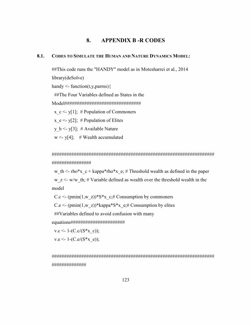
123

8. APPENDIX B -R CODES

8.1. CODES TO SIMULATE THE HUMAN AND NATURE DYNAMICS MODEL:

##This code runs the "HANDY" model as in Motesharrei et al., 2014

library(deSolve)

handy <- function(t,y,parms){

##The Four Variables defined as States in the

Model###############################

x_c <- y[1]; # Population of Commoners

x_e <- y[2]; # Population of Elites

y_h <- y[3]; # Available Nature

w <- y[4]; # Wealth accumulated

##################################################################

################

w_th <- rho*x_c + kappa*rho*x_e; # Threshold wealth as defined in the paper

w_z <- w/w_th; # Variable defined as wealth over the threshold wealth in the

model

C.c <- (pmin(1,w_z))*S*x_c;# Consumption by commoners

C.e <- (pmin(1,w_z))*kappa*S*x_e;# Consumption by elites

##Variables defined to avoid confusion with many

equations######################

v.c <- 1-(C.c/(S*x_c));

v.e <- 1-(C.e/(S*x_e));

##################################################################

##############

124

# Death rate of commoners and elites incluing the concept of

famine#############

alpha_c <- alpha.m + ((pmax(0,v.c,na.rm = TRUE))*

(alpha.M - alpha.m));

alpha_e <- alpha.m + ((pmax(0,v.e,na.rm = TRUE))*


##################################################################

###############

##State equations as in the paper that determine the simulation

xc_dot <- beta.c*x_c - alpha_c*x_c;

xe_dot <- beta.e*x_e - alpha_e*x_e;

yh_dot <- gamma*y_h*(lambda - y_h) - delta*x_c*y_h;

w_dot <- delta*x_c*y_h - C.c - C.e;

list(c(xc_dot,xe_dot,yh_dot,w_dot))

}

##################################################################

######################

assign("alpha.m",0.01); # [1/yr] normal (minimimum) death rate

assign("alpha.M",0.07); # [1/yr] Famine (maximum) death rate

assign("beta.c",0.03); # [1/yr] commoner birth rate

assign("beta.e",0.03); # [1/yr] elite birth rate

assign("S",5e-4); # [nature/(people * yr)] subsitence salary per people

assign("rho",5e-3); # [nature/people] subsitence salary per capita

assign("gamma",0.01); # [1/(nature * yr)] regeneration rate of nature

assign("lambda",100); # [nature] nature carrying capacity

assign("kappa",1); # Inequality factor (multiple of elite consumption per

assign("delta",6.67e-6); # [1/(commoner * yr)] depletion (production) factor

125

##################################################################

######################

xc_o <- 100;

xe_o <- 0;

yh_o <- lambda;

w_o <- 0;

##################################################################

######################

yini = c(xc_dot =xc_o,xe_dot = xe_o,yh_dot = yh_o,w_dot = w_o)

times <- seq(from = 0, to = 1000, by = 0.01)

handy_model <- ode(times = times,y = yini,

func = handy, method = c("ode45"), parms = NULL)

# Outputs from the function to be plotted

time <- handy_model[,1];

commoner_population <- handy_model[,2];

elite_population <- handy_model[,3];

nature <- handy_model[,4];

wealth <- handy_model[,5];

# Plotting equations

par(mfrow = c(2,2))#mar = c(2,2,2,2))

bmar <- 4 # Bottom margin (1)

lmar <- 5 # Left margin (2)

tmar <- 1 # Top margin (3)

rmar <- 1 # Right margin (4)

plot(time,commoner_population, type = "l",col = "blue",

xlab = "Time",ylab = "commoner_population",cex.lab=1.5,cex.axis=1.5 )

plot(time,elite_population, type = "l",col = "red",

xlab = "Time",ylab = "elite_population",cex.lab=1.5,cex.axis=1.5 )

126

plot(time,nature, type = "l",col = "green",

xlab = "Time",ylab = "nature",cex.lab=1.5,cex.axis=1.5 )

plot(time,wealth, type = "l",col = "black",

xlab = "Time",ylab = "wealth",cex.lab=1.5,cex.axis=1.5 )

8.2. CODES TO SIMULATE THE GOODWIN MODEL WITH DEBT AND WAGES BEING

MODELED EITHER ACCORDING TO THE LINEAR OR THE NONLINEAR FORM OF THE

PHILLIPS CURVE:

# This code simulates "The Goodwin Model" as in Keen, 2013 with and Without

Debt

# it also simulates its different forms i.e. the linear and the nonlinear form for the

Philip's Curve

##################################################################

###############################

## 1. type.wages = 1 simulates the Linear form for the Philip's Curve.

## 2. type.wages = 2 simulates the nonlinear form for the Philip's Curve.

## 3. type.debt = 1 simulates debt determined by the nonlinear investment curve

## 4. type.debt = 2 simulates no debt with linear relationship for Investments

#####################Where all profits are invested. Therefore, Invetments =

Profit

##################################################################

################################

library(deSolve)

goodwin <- function(t,y,parms){

#Various states defined in the goodwin model in Keen, 2013

a <- y[1];# Labor Productivity

Y <- y[2];# Output

N <- y[3];# Population

127

w <- y[4];# Real Wages

D <- y[5];# Debt

##################################################################

###############################

L <- Y/a;#labor

employment_rate <- L/N; # Employment Ratio (Lambda)

Wages <- (w)*(L); # Total Wages (Real Wages * Labor)

profit <- Y-Wages-r*D; # Profit

profit_rate <- (profit/(v*Y));# Profit Rate

##################################################################

###############################

if (profit >= 0) {

Invest_func <- (inv_yval - inv_min)*exp((inv_s/(inv_yval - inv_min))*

(profit_rate-inv_xval)) + inv_min;

} else {

Invest_func <- 0

}

##################################################################

######################################

if (type.wages==1) {

ph_func <- (-c+d*employment_rate);#Linear Philip's Curve

} else if (type.wages==2) {

ph_func <- (ph_yval - ph_min)*exp((ph_s/(ph_yval - ph_min)) *

(employment_rate - ph_xval)) + ph_min;# Nonlinear

Philip's Curve

}

##################################################################

######################################

128

#Equations that determine the simulations in the

model##################################################

a_dot <- alpha*a; # Labor Productivity

Y_dot <- ((Invest_func/v)-gamma_deprec)*Y;# Output

N_dot <- beta*N; # Population

w_dot <- ph_func*w; # Real Wages

##################################################################

################################

if (type.debt==1) {

Investment <- Invest_func*Y;# Nonlinear Investment Curve

} else if (type.debt==2) {

Investment <- profit; # Linear Investment, where All profits are

Invested###############

}

D_dot <- Investment - profit; # Debt

list(c(a_dot,Y_dot,N_dot,w_dot,D_dot));

}

##################################################################

############

assign("type.wages",2) # Linear or Nonlinear Philip's Curve

assign("type.debt",1) # Debt or No-Debt

assign("c",4.8); # Phlips Cuve = -c+d*Lambda

assign("d",5);

assign("v",3); # Accelerator

assign("alpha",0.02); # Labor Productivity Growth Rate

assign("beta",0.01); # Population Growt Rate

assign("gamma_deprec",0.01); # Depreciation Rate of Capital

assign("r",0.05); # Constant rate of Interest on Debt

129

##################################################################

#############

##Values for different Constants in the Nonlinear Philip's and Investment Curve

assign("ph_xval",0.95);

assign("ph_yval",0.0);

assign("ph_s",1.6);

assign("ph_min",-0.05);

assign("inv_xval",0.03333);

assign("inv_yval",0.1);

assign("inv_s",1*2.25);

assign("inv_min",0.0);

##################################################################

###############

###Setting initial conditions

a_o <- 1; # Initial Labor Productivity

N_o <- 100; # Intial Population

L_o <- 0.97*N_o;# Initial Labor

Y_o <- a_o*L_o; # Initial Output

D_o <- 0; # Initial Debt

w_o <- 0.88; # Initial Real Wage

##################################################################

#####################

yini <- c(a=a_o,Y=Y_o,N=N_o,w=w_o,D=D_o);

times <- seq(from = 0, to = 500, by = 0.01);

out <- ode(times = times, y = yini, func = goodwin, method = c("ode45"), parms

= NULL);

#output for the different states in the

model##########################################

130

time <- out[,1];

labor_productivity <- out[,2];

real_output <- out[,3];

population <- out[,4];

real_wages <- out[,5];

Debt <- out[,6];

##################################################################

#####################################

capital <- real_output*v;

labor <- real_output/labor_productivity;

profit <- real_output-(real_wages*labor)-r*Debt;

profit_rate <- (profit/(v*real_output));

employment_rate <- (labor/population);

wage_share <- 100*(real_wages/labor_productivity);

Debt_ratio <- Debt/real_output;


(employment_rate - ph_xval)) + ph_min;

Invest_func <- (inv_yval - inv_min)*exp((inv_s/(inv_yval -

inv_min))*(profit_rate-inv_xval)) + inv_min;

##################################################################

#####################################

#Plotting Different States in the

model#############################################################

###

par(mfrow = c(2,2))




131


par(mar=c(bmar,lmar,tmar,rmar))

plot(time,real_output,xlab = "Years",ylab = "Real

Output",type="l",cex.lab=1.5,cex.axis=1.5)

plot(time,labor,xlab = "Years",ylab = "Labor",type="l",cex.lab=1.5,cex.axis=1.5)

plot(time,population,xlab = "Years",ylab =

"Population",type="l",col="black",cex.lab=1.5,cex.axis=1.5)

plot(100*employment_rate,wage_share,xlab = "Employment Rate %",ylab =

"Wages share of output %",type = "l",col="black",cex.lab=1.5,cex.axis=1.5)

8.3. CODES TO SIMULATE THE MERGED MODEL (“HANDY” + “THE GOODWIN

MODEL”) WITH AND WITHOUT DEBT, WAGES BEING MODELED EITHER ACCORDING TO

THE LINEAR OR THE NONLINEAR FORM OF THE PHILLIPS CURVE, AND A NONLINEAR

INVESTMENT CURVE:

#This code is the master code for my thesis which has the ability to run the below

models

##################################################################

#######################

#1. Handy merged with Goodwin model with linear Phillips curve with either

Debt or No Debt

###1.1 Nature extraction as a function of Labor(L)

###1.2 Nature extraction as a function of Capital(K)

#2. Handy merged with Goodwin model with general exp form for Phillips

curve(Keen,2013) with either Debt or No Debt



###2.3 Nature extraction as a function of Power Input(pi)

132

#3. Handy merged with Goodwin model with general exp form for Phillips curve,

Debt/No debt with deprecitation of Wealth



###3.3 Nature extraction as a function of Power Input(pi)

library(deSolve)

goodwinhandy <- function(t,y,parms){

#State Variables

a <- y[1]; # Labor Productivity

w_h <- y[2]; # Wealth

Y <- y[3]; # Output

x_hc <- y[4];# Total Population

w <- y[5]; # Real wages

y_h <- y[6]; # Available Nature

D <- y[7]; # Debt

L <- Y/a; # Output

K <- Y*v; # Capital

##################################################################

#################

w_th <- rho*x_hc; # Threshold wealth as defined in the paper

w_z <- w_h/w_th; # Variable defined as wealth over the threshold wealth in the

model

C_hc <- (pmin(1,w_z))*S*x_hc;# Consumption by commoners

##Variables defined to avoid confusion with many

equations##########################

v.c <- 1-(C_hc/(S*x_hc));

133

##################################################################

##############

# Death rate of commoners and elites incluing the concept of

famine#############

alpha_hc <- alpha.m + ((pmax(0,v.c,na.rm = TRUE))*


##################################################################

###############

##################################################################

###########################

employment_rate <- L/x_hc; # Employment ratio

Wages <- (w)*(L); # Total wages (Real Wages* Labor)

profit <- Y-Wages-r*D; # Profit (Output - Total Wages - Intesrest paid on

Debt)

profit_share <- profit/Y; # Profit/Output

profit_rate <- profit_share/v; # Profit Share/v(Capital/Output)

wage_share <- Wages/Y; # Wages Share (Total Wages/ Output)

##################################################################

####################################

#Simulating different forms for the Phillips Curve either it's Linear or Nonlinear

form###############

if (type.wages==1) {

ph_func <- (-c+d*employment_rate);

} else if (type.wages==2) {

134


(employment_rate - ph_xval)) + ph_min;

}

##################################################################

#####################################

#########################NONLINEAR INVESTMENT

CURVE####################################################

Invest_func <- (inv_yval - inv_min)*exp((inv_s/(inv_yval -

inv_min))*(profit_rate-inv_xval)) + inv_min;

power_input = power_factor*w_h;

##################################################################

#####################################

####Nature Extraction as a function of Labor(L), Capital(K), Power

Input(Pi)###########################

if (type.extraction==1) {

nature_extraction <- delta_l*y_h*L; # Nature extraction as a function of Labor

} else if (type.extraction==2) {

nature_extraction <- delta_k*y_h*K; # Nature extraction as a function of

Capital

}else if(type.extraction==3){

nature_extraction <- delta_pi*y_h*power_input;

}

##################################################################

#####################################

135

########################################STATE

EQUATIONS################################################

##################################################################

#####################################

#With and Without Depreciation of

Wealth############################################################

###

if (type.deprec_h==1) {

w_h_dot <- nature_extraction - C_hc; # Change in Wealth without

Depreciation##########

} else if (type.deprec_h==2) {

w_h_dot <- nature_extraction - C_hc - deprec_h*w_h; # Change in Wealth

with Depreciation#############

}else if (type.deprec_h==3) {

w_h_dot <- nature_extraction - C_hc - power_input; # Change in Wealth when

Nature Extraction is a

##function of Power Input with no

Depreciation###

}else if (type.deprec_h==4) {

w_h_dot <- nature_extraction - C_hc - deprec_h*w_h-power_input;# Change

in Wealth when Nature

##Extraction is a function of

} ##Power Input with Depreciation

##################################################################

#####################################

if (type.debt==1) {

136

Investment <- Invest_func*Y;# Non linear Investment Function defined as in

Keen, 2013

} else if (type.debt==2) {

Investment <- profit; # Linear Investment, where investment = profit

}

a_dot <- alpha*a; # Labor productivity

Y_dot <- ((Investment/Y/v)-gamma_deprec)*Y; # Change in Output

x_hc_dot <- beta_hc*x_hc - alpha_hc*x_hc; # Change in Commoner

Population

w_dot <- ph_func*w; # Change in Real Wage according to the

Phillips Curve

y_h_dot <- gamma_hc*y_h*(lambda_h - y_h) - nature_extraction;# Change in

Available Nature

D_dot <- Investment - profit; # Change in Debt

list(c(a_dot,w_h_dot,Y_dot,x_hc_dot,w_dot,y_h_dot,D_dot));

}

assign("type.wages",2); # Linear or Nonlinear Phillips Curve

assign("type.extraction",3);

assign("type.debt",1); # Debt or No-Debt

assign("type.deprec_h",3) # Depreciation of Wealth at a Constant Rate

assign("rtype",5)

assign("ntype",2)

assign("pftype",5)

##################################################################

###########

#ASSIGN CONSTANT RATE OF INTERSET FROM 1% to 5% and 10%

seperately###########

137

##################################################################

###########

if (rtype==1) {

assign("r",0.01);

} else if (rtype==2) {

assign("r",0.02) ;

}else if(rtype==3){

assign("r",0.03);

}else if(rtype==4){

assign("r",0.04);

}else if(rtype==5){

assign("r",0.05);

}else if(rtype==10){

assign("r",0.1);

}

##################################################################

###########

#ASSIGN CONSTANT RATE OF INTERSET FROM 1% to 5% and 10%

seperately###########

##################################################################

###########

if (ntype==1) {

ef <- 0.5;

} else if (ntype==2) {

ef <-1 ;

}else if(ntype==3){

ef <- 2.5;

}else if(ntype==4){

138

ef <- 3.5

}else if(ntype==5){

ef <- 5

}

assign("delta_l",ef*6.67e-6); # [1/(population * yr)] depletion (production)

factor

assign("delta_k",ef*3.335e-07); # [1/(Capital * yr)] depletion (production) factor

assign("delta_pi",ef*0.3335); # [1/(power_input* yr)] depletion (production)

factor

if (pftype==1) { # % of wealth used as power to extract nature

assign("power_factor",0.01);

} else if (pftype==2) {


}else if(pftype==3){






}

assign("c",4.8); # Phlips Cuve = -c+d*Lambda

assign("d",5);

assign("deprec_h",0.01); # Rate at which accumulated wealth depreciates

assign("beta_hc",0.03); # Birth rate of the population

assign("gamma_hc",1e-2); # Regeneration rate of nature

assign("alpha.m",0.01); # [1/yr] normal (minimum) death rate

assign("alpha.M",0.07); # [1/yr] Famine (maximum) death rate

139

assign("S",5e-4); # [nature/(people * yr)] subsistence salary per people

assign("rho",5e-3); # [nature/people] subsistence salary per capita

assign("lambda_h",1*1e2); # [nature] nature carrying capacity

assign("v",3); # accelerator (= capital/output ratio)

assign("alpha",0.02); # rate of increase in labor productivity

assign("gamma_deprec",0.01);# depreciation rate of capital (%/yr)

##################################################################

#############

##Values for different Constants in the Nonlinear Phillips and Investment Curve

##################################################################

#############

assign("ph_xval",0.95);

assign("ph_yval",0.0);

assign("ph_s",1.6);

assign("ph_min",-0.05);

assign("inv_xval",0.03333);

assign("inv_yval",0.1);

assign("inv_s",1*2.25);

assign("inv_min",0.0);

##################################################################

##############

#SETTING INITIAL

CONDITIONS#####################################################

##################################################################

##############

a_o <- 1; # Labor Productivity

w_h_o <- 10; # Initial Wealth

x_hc_o <- 300; # Initial Population

140

y_h_o <- lambda_h; # Initial Nature

L_o <- 0.97*x_hc_o; # Initial Labor

Y_o <- L_o*a_o; # Initial Output (GDP)

D_o <- 0; # Initial debt

w_o <- 0.95; # Initial Real Wage

r_o <- r; # Initial Constant Rate of Interest

profit_o <- Y_o - w_o*L_o - r_o*D_o; # Initial Profits

yini <- c(a=a_o, w_h=w_h_o,Y=Y_o,x_hc=x_hc_o,w=w_o,y_h=y_h_o,D=D_o);

times <- seq(from = 0, to = 500, by = 0.01);

out <- ode(times = times, y = yini, func = goodwinhandy, method = c("ode45"),

parms = NULL);

##################################################################

##########################

#OUTPUT FOR DIFFERENT

VARIABLES######################################################

######

##################################################################

##########################

time <- out[,1];

labor_productivity <- out[,2];

wealth <- out[,3];

real_output <- out[,4]

population <- out[,5];

real_wages <- out[,6];

nature <- out[,7];

Debt <- out[,8];

labor <- real_output/labor_productivity;

lambda <- labor/population;

141

debt_ratio <- Debt/real_output;

capital <- real_output*v;

wage_share <- (real_wages/labor_productivity)*100;

employment_rate <- (labor/population)

profit_share <- (real_output - real_wages*labor - Debt*r)/real_output;

profit <- real_output - (real_wages*labor) - (r*Debt);

profit_share <- profit/real_output

profit_rate <- profit_share/v;

##################################################################

#############

# (3) Define plot arrangement and margins (in inches)

par(mfrow = c(4,2))





# Define plot margins and axis tick label placement




plot(time,wealth,xlab = "Years",ylab =

"Wealth",type="l",cex.lab=1.5,cex.axis=1.5)


"Population",type="l",cex.lab=1.5,cex.axis=1.5)

plot(time,nature,xlab = "Years",ylab = "Nature",type =

"l",cex.lab=1.5,cex.axis=1.5)

plot(time,debt_ratio,xlab = "Years",ylab="Debt Ratio",type =


142

plot(time,profit_rate,xlab = "Years",ylab = "Profit

Rate",type="l",cex.lab=1.5,cex.axis=1.5)

plot(time,wage_share,xlab="Years",ylab = "Wage

Share",type="l",cex.lab=1.5,cex.axis=1.5)

plot(time,employment_rate*100,xlab = "Years",ylab = "Employment Rate

(%)",type="l",cex.lab=1.5,cex.axis=1.5)

##################################################################

##########################################

#plot(time,capital,xlab = "years",ylab = "Capital",type = "l")

#plot(employment_rate*100,100*ph_func,xlab = "employment rate (%)",ylab =

"Annual change in real wage(%)",type = "l")#,xlim = c(95,100),ylim = c(0,20))

#plot(profit_rate*100,Invest_func*100,xlab = "profit rate(%)",ylab = "Investment

as % of Output",type = "l",xlim = c(0,10),ylim = c(0,20))

#plot(employment_rate*100,wage_share,xlab = "employment rate(%)",ylab =

"Wage share of output(%)",type = "l",cex.lab=1.5,cex.axis=1.5)

#title(main="Merged Model @ Constant r= 4.5%,L^.3K^.3a^.4", outer = TRUE,

cex =0.5, line = -1)

#plot(time,labor_productivity,xlab = "years",ylab = "labor productivity",type="l")

#plot(time,labor,xlab = "years",ylab = "labor",type="l")

#plot(time,Debt,type = "l",xlab = "years",ylab = "Debt")

#plot(time,r,xlab = "years",ylab = "rate of interest",type = "l")

#plot(employment_rate,ph_func_test,xlab = "emplotyment rate

(%)",ylab="Phillps Curve Output (change in wages)",type = "l")

#plot(time,ph_func_test,xlab = "Years",ylab="Phillps Curve Output (change in

wages)",type = "l")

#plot(profit_rate,Invest_func_test,xlab = "Profit Rate",ylab="Investment fraction

of output",type = "l")

if (ntype==1) {

143

par(mfrow = c(3,2))







plot(time,wealth,xlab = "Years",ylab = "Wealth

Accumulated",type="l",cex.lab=1.5,cex.axis=1.5)











n_DR_1 <- data.frame(debt_ratio)

write.csv(n_DR_1,file = "Debt Ratio@n=1.csv")

n_P_1 <- data.frame(population)

write.csv(n_P_1,file = "Population@n=1.csv")

n_N_1 <- data.frame(nature)

write.csv(n_N_1,file = "Nature@n=1.csv")

n_O_1 <- data.frame(real_output)

write.csv(n_O_1,file = "Output@n=1.csv")

144

} else if (ntype==2) {

par(mfrow = c(3,2))


























145


} else if (ntype==3){

par(mfrow = c(3,2))

























146



} else if (ntype==4){

par(mfrow = c(3,2))
























147




} else if(ntype==5){

par(mfrow = c(3,2))























148





}

##################################################################

################

if (rtype==1) {

par(mfrow = c(3,2))



















149

r_DR_1 <- data.frame(debt_ratio)

write.csv(r_DR_1,file = "Debt Ratio@r=1%.csv")

r_P_1 <- data.frame(population)

write.csv(r_P_1,file = "Population@r=1%.csv")

r_N_1 <- data.frame(nature)

write.csv(r_N_1,file = "Nature@r=1%.csv")

r_O_1 <- data.frame(real_output)

write.csv(r_O_1,file = "Output@r=1%.csv")

} else if (rtype==2) {

par(mfrow = c(3,2))

















150











} else if (rtype==3){

par(mfrow = c(3,2))















151













} else if (rtype==4){

par(mfrow = c(3,2))













152















} else if(rtype==5){

par(mfrow = c(3,2))











153

















}else if (rtype==10) {

par(mfrow = c(3,2))









154



















}

if (pftype==1) {

par(mfrow = c(3,2))







155













pf_DR_1 <- data.frame(debt_ratio)

write.csv(pf_DR_1,file = "Debt Ratio@pf=1.csv")

pf_P_1 <- data.frame(population)

write.csv(pf_P_1,file = "Population@pf=1.csv")

pf_N_1 <- data.frame(nature)

write.csv(pf_N_1,file = "Nature@pf=1.csv")

pf_O_1 <- data.frame(real_output)

write.csv(pf_O_1,file = "Output@pf=1.csv")

} else if (pftype==2) {

par(mfrow = c(3,2))






156






















} else if (pftype==3){

par(mfrow = c(3,2))





157























} else if (pftype==4){

par(mfrow = c(3,2))





158























} else if(pftype==5)

par(mfrow = c(3,2))




159
























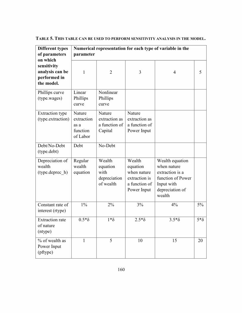
160

TABLE 5. THIS TABLE CAN BE USED TO PERFORM SENSITIVITY ANALYSIS IN THE MODEL.

Different types

of parameters

on which

sensitivity

analysis can be

performed in

the model.

Numerical representation for each type of variable in the

parameter

1

2

3

4

5

Phillips curve

(type.wages)

Linear

Phillips

curve

Nonlinear

Phillips

curve

Extraction type

(type.extraction)

Nature

extraction

as a

function

of Labor

Nature

extraction as

a function of

Capital

Nature

extraction as

a function of

Power Input

Debt/No-Debt

(type.debt)

Debt No-Debt

Depreciation of

wealth

(type.deprec_h)

Regular

wealth

equation

Wealth

equation

with

depreciation

of wealth

Wealth

equation

when nature

extraction is

a function of

Power Input

Wealth equation

when nature

extraction is a

function of Power

Input with

depreciation of

wealth

Constant rate of

interest (rtype)

1% 2% 3% 4% 5%

Extraction rate

of nature

(ntype)

0.5*δ 1*δ 2.5*δ 3.5*δ 5*δ

% of wealth as

Power Input

(pftype)

1 5 10 15 20

161

8.3.1. CODES TO READ .CSV OUTPUT FILES FROM THE PREVIOUS CODE IN SECTION 8.3

#This code reads the .CSV output files and combines them to create plots to run

sensitivity

##analysis on Debt Ratio, Population, Nature, and Output.

DR1 <- read.csv("Debt Ratio@pf=1.csv")





DRCombined <- cbind(DR1,DR2,DR3,DR4,DR5)

DR_C <- data.frame(DRCombined)

write.csv(DR_C,file = "DebtRatioCombined.csv")

####################################################

p1 <- read.csv("Population@pf=1.csv")





pCombined <- cbind(p1,p2,p3,p4,p5)

p_C <- data.frame(pCombined)

write.csv(p_C,file = "populationCombined.csv")

####################################################

n1 <- read.csv("Nature@pf=1.csv")





nCombined <- cbind(n1,n2,n3,n4,n5)

162

n_C <- data.frame(nCombined)

write.csv(n_C,file = "natureCombined.csv")

#####################################################

o1 <- read.csv("Output@pf=1.csv")





oCombined <- cbind(o1,o2,o3,o4,o5)

o_C <- data.frame(oCombined)

write.csv(o_C,file = "outputCombined.csv")

8.3.2. PLOTTING CODES FOR THE MERGED CSV’S FROM SECTION 8.3.1

#This code plots the CSV outputs from the previous code, it's important to make

sure that

##the CSV's do not contain the time column more than once before running the

code.

debtratio <- read.csv("DebtRatioCombined.csv")

population <- read.csv("populationCombined.csv")

Nature <- read.csv("natureCombined.csv")

Output <- read.csv("outputCombined.csv")

par(mfrow = c(2,2))





#

# # # Define plot margins and axis tick label placement

163


matplot(debtratio[,1]/100,debtratio[,-1],type = "l",lty=1,lwd =2,xlab =

"Years",ylab = "Debt Ratio",col = c("black","blue","red","green","brown"),ylim =

c(0,5e4),xlim = c(0,500),cex.lab=1.5,cex.axis=1.5)

legend(150,5e4,legend=c("1%", "5%","10%","15%","20%"),lty=1, cex=0.8,col =

c("black","blue","red","green","brown"))

matplot(population[,1]/100,population[,-1],type = "l",lty=1,lwd =2,xlab =

"Years",ylab = "Population",col =

c("black","blue","red","green","brown"),cex.lab=1.5,cex.axis=1.5)#,ylim =

c(0,8e4))#,xlim = c(0,300))

legend(0,5.5e4,legend=c("1%", "5%","10%","15%","20%"),lty=1, cex=0.8,col =


matplot(Nature[,1]/100,Nature[,-1],type = "l",lty=1,lwd =2,xlab = "Years",ylab =

"Available Nature",col =

c("black","blue","red","green","brown"),cex.lab=1.5,cex.axis=1.5)#,xlim =

c(0,300))

legend(100,90,legend=c("1%", "5%","10%","15%","20%"),lty=1, cex=0.8,col =


matplot(Output[,1]/100,Output[,-1],type = "l",lty=1,lwd =2,xlab = "Years",ylab =

"Output",col = c("black","blue","red","green","brown"),ylim =

c(0,2e8),cex.lab=1.5,cex.axis=1.5)#,xlim = c(0,300))

legend(0,2e8,legend=c("1%", "5%","10%","15%","20%"),lty=1, cex=0.8,col =


title(main = "Effect of Constant Rate of Interest", outer = TRUE, cex =2.5, line =

-1 )

#legend(10,5,lty=c(1,1),lwd=c(2.5,2.5))

#legend(0,1e09,legend=c("Line 1", "Line 2"),lty=1:2, cex=0.8)

164

9. REFERENCE

Acemoglu, Daron. 2009. "The Solow Growth Model." Introduction to Modern Economic

Growth 26-76.

Antón, Susan C., and Carl C. Swisher III. 2005. "Early Dispersals of homo from Africa."

Annual Review of Anthropology 271-296.

Arrow, K. J., H. B. Chenery, B. S. Minhas, and R. M. Solow. 1961. "Capital-labor

substitution and economic efficiency." Review of Economics and Statistics (The

MIT Press) 225-250.

Chen, J. 2016. The Unity of Science and Economics. New York: Springer-Verlag.

Cobb, C. W., and P. H. Douglas. 1928. "A Theory of Production." American Economic

Review 139-165.

Dixon, H. 1999. "New Keynesian Economics, nominal rigidities and involuntary

unemployment." Journal of Economic Methodology 221-238.

Dodson. 2004. 46.

Domar, Evsey. 1946. "Capital Expansion, Rate of Growth, and Employment."

Econometrica.14(2) 137-147.

Douglas, Paul H. 1976. "The Cobb-Douglas Production Function Once Again: Its

History, Its Testing, and Some New Empirical Values." Journal Political

Economy 84.

Foley, K. D., and T. Michl. 1999. Growth and Distribution. Cambridge, MA: Harvard

University Press.

Godley, Wynne, and Marc Lavoie. 2006. Monetary Economics: "An Integrated Approach

to Credit, Money, Income, Production and Wealth. palgrave Macmillan.

Goodwin, R.M. 1967. A Growth Cycle. Edited by C.H. Feinstein. Cambridge: Cambridge

University Press.

Harrod, Roy F. 1939. "An Essay in Dynamic Theory." The Economic Journal. 49 (193)

14-33.

Jorgensen, Dale W. 2000. Econometrics, vol 1: Econometric Modelling of Producer

Behavior. Cambridge: The MIT Press.

Keen, S. 2013. "A Monetary Minsky Model of the Great Moderation and the Great

Recession." Journal of Economic Behavior & Organization 221-235.

165

Keen, S. 2013a. "A Monetary Minsky Model of the Great Recession." Journal of

Economic Behavior & Organization, 86 221-235.

Keen, S. 1995. "Finance and Economic Breakdown: Modeling Minsky's "Financial

Instability Hypothesis" ." Journal of Economic Behavior & Organization, 86 221-

235.

Keen, S. 2009. "Neoclassical Economics: mad, bad, and dangerous to know." Steve

Keen's Debtwatch.

Keynes, John Maynard. 1936. The general theory of employment, interest, and money.

London: Macmillan.

King, C. W. 2015b. "The Rising Cost of Resources and Global Indicators of Change."

American Scientist 103.

Klump, R., A. William, and P. McAdam. 2007. "Factor Substitution and Factor

Augmenting Technical Progress in the US: A Normalized Supply-Side

Approach." Review of Economics and Statistics 183-192.

Lifshitz, Michail. 1948. "Giambattista Vico (1668-1744)." Philosophy and

Phenomenological Research 8.3 391-414.

Lotka, Alfred J. 1925. Elements of Physical Biology. Williams and Wilkins.

Malmström, Vincent H. 2014. "The Maya Inheritance."

Meadows, Donella H., Dennis L. Meadows, Jorgen Randers, and Willian W. Behrens III.

1972. The Limits to Growth. 1972 Universe Books.

Mitchell, T. 2013. Carbon Democracy: Political Power in the Age of Oil. London and

New York: Verso.

Morgan, David. 2007. The Mongols, 2nd Edition. Wiley-Blackwell.

Morgan, Mary S. 2008. "models." The New Palgrave Dictionary of Economics, 2nd

Edition.

Morris, Ian. 2010. Why the West Rules - For Now: The Patterns of History, and What

They Reveal About the Future. New York: Farrar, Straus, and Giroux.

Motesharrei, S., J. Rivas, and E. Kalnay. 2014. "Human and Nature Dynamics

(HANDY): Modeling inequality and use of resources in the collapse or

sustainability of societies." Ecological Economics, 101 90-102.

166

Phillips, A. W. 1958. "The Relationship between Unemployment and the Rate of Change

of Money Wages in the United Kingdon 1861-1957." Economica.25(100) 283-

299.

Pindyck, R.S. 2013. "Climate Change Policy: What Do the Models Tell Us?" Journal of

Economic Literature, 51 860-872.

Samuelson, P.A. 1939. "Interactions Between the Multiplier Analysis and the Principle of

Acceleration." Review of Economic Statistics 75-78.

Solow, Robert M. 1956. "A contribution to the theory of economic growth." Quarterly

Journal of Economics. Oxford Journals. 70(1) 65-94.

Stanford, James. 1993. "Continental Economic Integration: Modeling the Impact on

Labor." Annals of the American Academy of Political and Social Science 92-110.

Stern, N. 2013. "The Structure of Economic Modeling of the Potential Impacts of

Climate Change: Grafting Gross Underestimation of Risk onto Already Narrow

Science Models." Journal of Economic Literature, 51 838-859.

Swan, Trevor W. 1956. "Economic growth and capital accumulation." Economic Record

334-361.

Tainter, J. A., T. F. H. Allen, A. Little, and T. W. Hoekstra. 2003. "Resource Transitions

and Energy Gain: Contexts of Organization." Conservation Ecology,7.

Tainter, Joseph A. 2011. "Energy, Complexity, and Sustainability: A Historical

Perspective." Environmental Innovation and Societal Transitions (Cambridge

University Press) 89-195.

Tainter, Joseph A. 1988. The Collapse of Complex Societies. Cambridge University

Press.

Trinkaus, Erik. 2005. "Early Modern Humans." Annual Review of Anthropology 207-

230.

Turchin, P., and S. A. Nefedov. 2009. Secular Cycles. Princeton University Press.

Turchin, P., T.E. Currie, E.A.L. Turner, and S. Gavrilets. 2013. "War, space, and the

evolution of Old Worlds complex societies." Proceedings of the National

Academy of Sciences 110.

Wright, Rita P. 2009. "The Ancient Indus: Urbanism, Economy, and Society."

copyright by harshit jayaswal 2017

Documents