Cooperative Search and Survey using Autonomous

Underwater Vehicles (AUVs)

Seokhoon Yoon and Chunming Qiao

Department of Computer Science and Engineering

State University of New York at Buffalo

Email: {syoon4,qiao}@cse.buffalo.edu

Abstract—In this work, we study algorithms for cooper-

ative search and survey using a fleet of AUVs (Autonomous

Underwater Vehicles). Due to the limited energy, commu-

nication range/bandwidth, and sensing range of the AUVs,

underwater search and survey with multiple AUVs brings

about several new challenges when a huge amount of data

needs to be collected, and any AUV may fail unexpectedly.

To address the challenges and meet our objectives of

minimizing the total travel time and distance of AUVs,

we first study a simple strategy called Lane Based Search

(LBS). Then, we propose a cooperative rendezvous scheme,

X Synchronization (XS), which enables AUVs to coordinate

their data aggregation, control signal dissemination, and

AUV failure detection/recovery operations via mobility-

assisted data communication. We also devise a way to

calculate appropriate timeout periods used to detect an

AUV failure and describe how surviving AUVs subse-

quently carry out the survey mission. Numerical analysis

and simulations have been performed to compare the

performance of XS and other rendezvous schemes. The

results show that XS can outperform other rendezvous

schemes in terms of the total survey time and the travel

distance of AUVs.

I. INTRODUCTION

Recent development in technology of acoustic and

magnetic sensors, underwater communication devices,

and especially autonomous underwater vehicles has en-

abled comprehensive underwater monitoring for various

applications. In this paper, we propose an architecture

for cooperative search and survey using a fleet of AUVs.

This work targets the time-sensitive search and surveying

applications (e.g. underwater surveillance, search/rescue

operation, or seismic monitoring) in a large area without

using any pre-existing infrastructure such as observa-

tory/cabling, while at the same time, requiring the ability

to deal with possible AUV failures.

A. Design Consideration

Given the targeted applications, our major design

considerations include

• Load Balancing and Energy Efficiency: Since AUVs

have limited energy source, the amount of search

and survey load (in terms of area or distance cov-

ered) should be evenly distributed among AUVs.

Also, the total search and survey distance and time

should be minimized to achieve overall efficiency.

• Directional Search: In a search or rescue operation,

directional search is desirable especially in the

presence of a strong underwater current. The fleet

of AUVs should begin a survey from a position,

where a target (e.g. a wrecked ship/airplane) is

likely located, to the direction in which the target is

likely to move. Further, even for a normal survey,

surveying in the same direction of the underwater

current will be more energy efficient.

• Fault Tolerance: The fleet of AUVs are required to

complete the survey in the presence of AUV failures

due to a mechanical and/or communication prob-

lem. Therefore, AUVs should perform the failure

detection/recovery as soon as possible to minimize

the survey completion time.

• Data Aggregation and Control Signal Disseminia-

tion: For timely reaction to intermediate findings

during search and survey, data collected by AUVs

need to be aggregated and sent to either one or

more specially equipped AUVs or a mothership

(or basestation) for analysis. The need for data

aggregation may also arise due to the fact that

the AUVs may have a limited storage capacity on

board due to size, weight, and power consideration,

especially if high resolution data (e.g. high quality

video or photo image) is to be collected over a large

area. In such a case, data aggregation can alleviate

the problem since data can be consumed (or at least

compressed) by a sink node (e.g. a powerful AUV

or mothership). Conversely, during the search and

survey process, control signals (including requests

and commands) from the mothership or an AUV

may need to be disseminated to other AUVs to

respond to certain events (which may or may not

be triggered by the intermediate findings).

As to be discussed in Section II, existing approaches

relying on a single AUV or infrastructure (e.g. cabling

and fixed observatories) for underwater monitoring are

no longer effective for the targeted applications. In

addition, no existing works using cooperative mobile

nodes take the above design considerations into account.

B. Overview

Based on the design considerations discussed above,

instead of requiring the fleet of AUVs to be connected

to each other and in particular be in a certain formation

as in previous works on cooperative mobile nodes, we

consider a simple survey strategy, Lane Based Search

(LBS). In LBS, the survey area is partitioned into sev-

eral sub-areas, each being assigned to one AUV, which

collects data of interest (e.g. bathymetric mapping data

or photo/video image) in the sub-area in the appropriate

direction. Note that, given a large area and a small

number of AUVs, the width of each sub-area may exceed

the communications (and sensing) range of each AUVs.

Accordingly, this differentiates our work from those

requiring the fleet of AUVs to be connected to each other

and in particular be in a certain formation as in previous

works on cooperative mobile nodes.

Each AUV is assumed to be able to calculate its

location using onboard sensors (e.g. Doppler Velocity

Log, a gyrocompass, and a pressure sensor) based on its

previously known location (e.g., the point of the initial

deployment). To minimize the positioning error, each

AUV periodically updates its location via an acoustic

signal from a mothership [1] or other AUVs that have

recently updated their locations. We also consider the

possibility that one or more AUVs may have more

powerful computing resources for data analysis, or can

communicate with the mothership via a long range

acoustic channel (or an optical cable) to send collected

data and receive control signals. Such a powerful AUV

will become the Lead AUV and the rest become Member

AUVs of the fleet. This is illustrated in Fig. 1. Note

that our scheme, to be described in more detail below,

will still be useful even if all AUVs are equal and there

is no mothership since coordination among AUVs via

control signal dissemination for AUV failure resilience

for example is still needed.

More specifically, for failure detection/recovery of

AUVs, data aggregation, and other coordinated oper-

ations, AUVs need to communicate with each other.

However, the width of each sub-area can be wider than

the data communication range of each AUVs due to

limitations of underwater communication [2]–[4]. Even

the two AUVs assigned to the neighboring sub-areas may

not be able to transfer data with each other at all times,

except when they move close to each other towards

the common border. For instance, to achieve 500 kbps

data rate, the distance between two communicating peers

should be less than or around 60 meters in a deep water

by using PSK modulation technique [3]. Alternative

communication technologies also require short transmis-

sion range for a higher data rate (e.g. 10 Mbps data

rate can be achieved with a transmission range about 20

meters using underwater optical link [5]). Accordingly,

the AUVs form a intermittently connected network (ICN)

or disruption/delay tolerant network (DTN) in which

the AUVs are not always connected to one another.

Therefore, the main challenges are to enable AUVs to

perform mass data communication (or control signal dis-

semination) without significantly increasing energy con-

sumption and survey completion time in the ICN/DTN

environment, and to survive possible AUV failures.

To address the above challenges, we propose a coop-

erative rendezvous schemes, X Synchronization (XS), in

which AUVs periodically meet for synchronization while

surveying an area. During synchronization, data and con-

trol signals including updated positioning information

are relayed among AUVs via mobility-assisted commu-

nication in a multi-hop fashion. XS enables AUVs to

perform synchronization without any extra movement,

as AUVs determine the RP (Rendezvous Point) where

synchronization occurs along the survey path. In addi-

tion, XS allows AUVs to determine the frequency of

synchronization such that the survey completion time is

minimized. XS also provides resilience to AUV failures

by detecting the failure and then covering the sub-area

allocated to the failed AUV with the surviving AUVs.

As shown in Fig. 1, each AUV performs the survey

and, when an AUV moves close to its neighbor, it

forwards sensor data or control signal to the neighbor.

For example, the sensor data that A5 has collected is

forwarded to A4 at T1. Then, at T2, the data is again

forwarded to A3 (Lead AUV) where sensor data is

aggregated. In a similar way, the control signals are

disseminated from the Lead AUV to the member AUVs.

In this work, we also determine appropriate synchro-

nization timeout values to be used in XS to reduce the

number of false alarms while being able to detect actual

failures as soon as possible. A numerical model is also

devised to approximate the survey time and traveling dis-

tance, and verified through simulations. Both numerical

analysis and simulation results show that XS outperforms

two other rendezvous algorithms, Alternating Columns

Synchronization (ACS) and Strict Line Synchronization

(SLS) which we have also considered.

The rest of the paper is organized as follows. Section

II discusses related works. In Section III, a basic survey

architecture including LBS is described. Section IV

introduces other rendezvous schemes and presents the

proposed XS. Section V derives an appropriate timeout

period for failure detection. Sections VI and VII eval-

uate the performance of XS through numerical analysis

and simulations respectively. Section VIII concludes the

paper.

II. RELATED WORKS

A. Oceanographic Monitoring

Recently, many underwater observation projects have

been carried out using new technologies (e.g. sen-

sors, acoustic communication, and AUVs), which have

enabled scientists to pursue new approaches to the

Fig. 1. Underwater survey with cooperative AUVs

oceanography studies.

The projects in [6], [7] established a long term un-

derwater observatory. In particular, the Neptune project

[6] established a plate-scale fiber-optic/power cable con-

nected undersea observatory network on the Juan de

Fuca tectonic plate. The electro/optical cable provides

high power and communication bandwidth to the ob-

servatories for real-time and long-term four dimensional

remote oceanographic studies (e.g. ocean dynamics,

marine organisms, plate tectonics, and biogeochemical

cycles). Thirty Neptune nodes are spaced approximately

100 km apart which leads to thousands of kilometers

of cable length in a mesh topology. The network of

those nodes serves as a fixed infrastructure for the

oceanography studies. In contrast, our work focuses on

the flexible, short-term, and on-demand oceanographic

monitoring problem in areas without infrastructure.

The works in [8], [9] used a single AUV for the

oceanographic study. In [8], an AUV is deployed for

45 hours to survey a 48km2 coral mound field in the

Straits of Florida, while in [9] an AUV, which carries

various sonar magnetic and camera based sensors, had

to make 165 dives to survey a distance of about 2500 km

for the seafloor dynamics study [10], [11]. Accordingly,

they are applicable to a relatively small area or relatively

long-term project. Meanwhile, our work focuses on the

time-sensitive search and survey applications in a large

area using multiple cooperative AUVs.

In [12], authors reported the experimental results from

using three AUVs in Monterey Bay based on adapt-

able formation control of constantly-connected AUVs

(instead of intermittently connected AUVs studied in our

work). It also differs from ours in that their works focus

on the gradient climbing and feature tracking problem

instead of minimization of the survey time and traveling

distance.

B. Underwater Communication and Networking

There have been a lot of works on underwater com-

munication and networking [2]–[5], [13]–[15]. [2]–[4]

studied issues of designing reliable underwater acous-

tic networks. In particular, the work in [2] discussed

the challenges of underwater networking due to power

limitation and the underwater acoustic communication

characteristics such as limited bandwidth, high level of

multi-path effect and fading, high propagation delay and

bit error. The study in [3] summarized the development

of modulation techniques and corresponding achievable

data rates and transmission ranges. [3] also discussed

disadvantages of acoustic channel for a long distance

communication, and proposed to use short-range under-

water acoustics based multi-hop acoustic network. In [4],

it was shown that multi-hop underwater communication

can be more energy efficient than a long single hop

communication.

Alternative underwater communication technologies

have also been studied for short-range high data rate

communication [5], [16], [17]. [5] showed that up to

10 Mbps data rate can be achieved for the range of 20m

using directed light transmitters. [16] studied preliminary

design of optical communication system using omnidi-

rectional optical transceiver to achieve up to 10Mbps

data rate. [17] studied underwater communication based

on electric current for low power and short distance com-

munication, and showed that it can potentially achieve

about 1 Mbps data rate. These and other related studies

show that our assumptions on limited sensing and (high

data rate) communications ranges are reasonable.

C. Cooperative Operation of Mobile Nodes

There also have been studies on applications of mobile

sensor nodes. The works in [18] [19] studied movement

assisted sensor deployment, [20] showed mobile sensor

nodes increases the sensing coverage, and [21] studied

a triangulation-based sensor coverage algorithm using

three mobile sensor nodes. Individual mobile sensor

node technologies such as AUVs [22], UAVs (Unmanned

Aerial Vehicle) [23], and autonomous vehicles [24] also

have been studied.

The works in [25]–[27] studied natural phenomenon

of cooperative flocking or swarming. [28], [29] proposed

algorithms for cooperation of mobile nodes inspired

by those biological behaviors. [30] proposed a team

Surv

ey

1

2

3

4

lane1· · ·

lanen

···

L

lane2

Rr

h ≤ 2r

wlevel

fleet of AUVs

Survey Region

(a)

r

2rn

· · ·

(b)

Fig. 2. Oceanographic Survey Strategy: Lane Based Search

architecture of robotic agents for surveillance in a small

area (office or lab environment) where ranger nodes carry

and deploy a set of scout nodes that have a video camera

and motion detector.

However, these works assume that mobile nodes form

a constantly connected network, while in our work AUVs

form a delay tolerant network. In addition, none of these

works addressed the survey problem in a large area using

a potentially large number of cooperative mobile nodes.

III. UNDERWATER SURVEY: BASIC ARCHITECTURE

In this section, we discuss the basic underwater survey

architecture. We first describe the Lane Based Search

strategy where each AUV is assigned to an equal sized

sub-area. Then, we introduce synchronization among

AUVs which enables AUVs to employ mobility-assisted

communication for coordinated operations including sen-

sor data aggregation, control signal dissemination, and

detection/recovery of AUV failures.

A. Lane Based Search

Fig. 2 shows an example of oceanographic survey

along the mid-ocean ridge [31] to obtain ocean bathymet-

ric data (e.g. volcanic tectonic features, ocean morphol-

ogy, or hydrothermal vents). In our survey architecture,

one or more survey regions are first determined as shown

in Fig. 2. The properties of each survey region (such

as location, size, and shape) depend on many factors

including the purpose of the survey, the number of

AUVs, and battery life of each AUV. Determination of

survey regions are beyond the scope of this work, and

we assume that survey regions are given.

Lane Based Search (or LBS) strategy is used to cover

each survey region as shown in Fig. 2 (a). A survey

region of H x W units is partitioned into n sub areas

of equal size, where n is the number of AUVs. Each

sub area, called a lane hereafter, is H x w units where

w = Wn (the width of a lane). Each AUV is assigned to

one lane, and an AUV is responsible for surveying its

designated lane. Let r be the sensing range of each AUV.

If the width of lane, w, is less than 2r (the survey swath

of each AUV), AUVs move only forward in the survey

direction. In practice, in a large survey area, however, w

can be much larger than 2r. In that case, an AUV has

to move horizontally as well as forward (following a

snake like path) as illustrated in Fig. 2. The survey area

can thus be considered to have multiple levels length-

wise, and the height of each level, h, has to be less

than or equal to 2r to avoid any sensing coverage hole.

In addition, since the width of a lane can also be wider

than the data transmission range, R, an AUV has to move

close to the borders of its lane in order to communicate

with its neighboring AUVs for relaying data.

An alternative survey strategy is that the AUVs move

in a formation (e.g., a simple line) to sweep the area

either vertically or horizontally. In other words, as shown

Fig. 2 (b), the entire formation moves in the same snake-

like fashion (in sync with each other) as each individual

AUV does in LBS except that the width of the “lane” as-

signed to each AUV in this alternative approach is much

narrower than in our approach. Note that, in practice, it

is very difficult to maintain a formation as it requires

each AUV to make constant adjustments to keep in sync

with each other. In addition, this alternative approach

may not be effective for the problem under consideration.

For example, when the (data) communication range of an

AUV is smaller than the swath width as determined by

the sensing range r of the AUV (i.e. R < 2r), keeping

the AUVs close to each other in order to maintain the

formation will result in overlapped sensing areas which

may be unnecessary and thus resulting in an overhead.

In addition, the alternative strategy may require more

energy consumption especially for a large survey area.

To compare the energy consumption of the LBS and the

alternative strategy, we derive a simple energy consump-

tion model based on the traveling distance of the AUVs.

For simplicity, suppose a square survey region of W x

W units and all AUVs are initially deployed at their

starting point by mothership. Also let d = 2r.

In LBS, the region is partitioned into n lanes, each of

which has a width of Wn . For the survey, an AUV first

moves the distance of Wn −d for the horizontal survey at

each level (note that an AUV does not need to move up to

the border line of lanes due to the sensing range r). Then,

it moves vertically to the next level. The total number of

levels is Wd , and the total travel distance for the vertical

movements is W − d for each AUV. Therefore, the total

traveling distance of all AUVs, Slbs, becomes

Slbs = n

(W

d

(W

n− d

)+ W − d

)(1)

=W 2

d− nd (2)

When the alternative approach is used, the fleet of AUVs

have the vertical survey as many as⌈

Wdn

⌉times, which

results in the total distance of (W − d) × ⌈Wdn

⌉for the

vertical survey of each AUV. After a vertical survey,

each AUV moves horizontally by the distance of dn.

During survey, each AUV has the horizontal movements

as many as⌈

Wdn − 1

⌉times. For simplicity, let W

dn be

an integer number. Then, the total traveling distance of

AUVs becomes

Salt = n

[(W − d)× W

dn+ dn

(W

dn− 1

)](3)

=W 2

d+ (n− 1)W − dn2 (4)

Suppose that both LBS and the alternative approach

consume the same amount of energy for traveling a

unit distance. Then, to compare the energy consumption

between two approaches, we show Salt − Slbs > 0.

Note that Wdn ≥ 2 i.e. W ≥ 2dn (if W

dn = 1, the LBS

and the alternative approach will have the same survey

path, which will result in the same traveling distance).

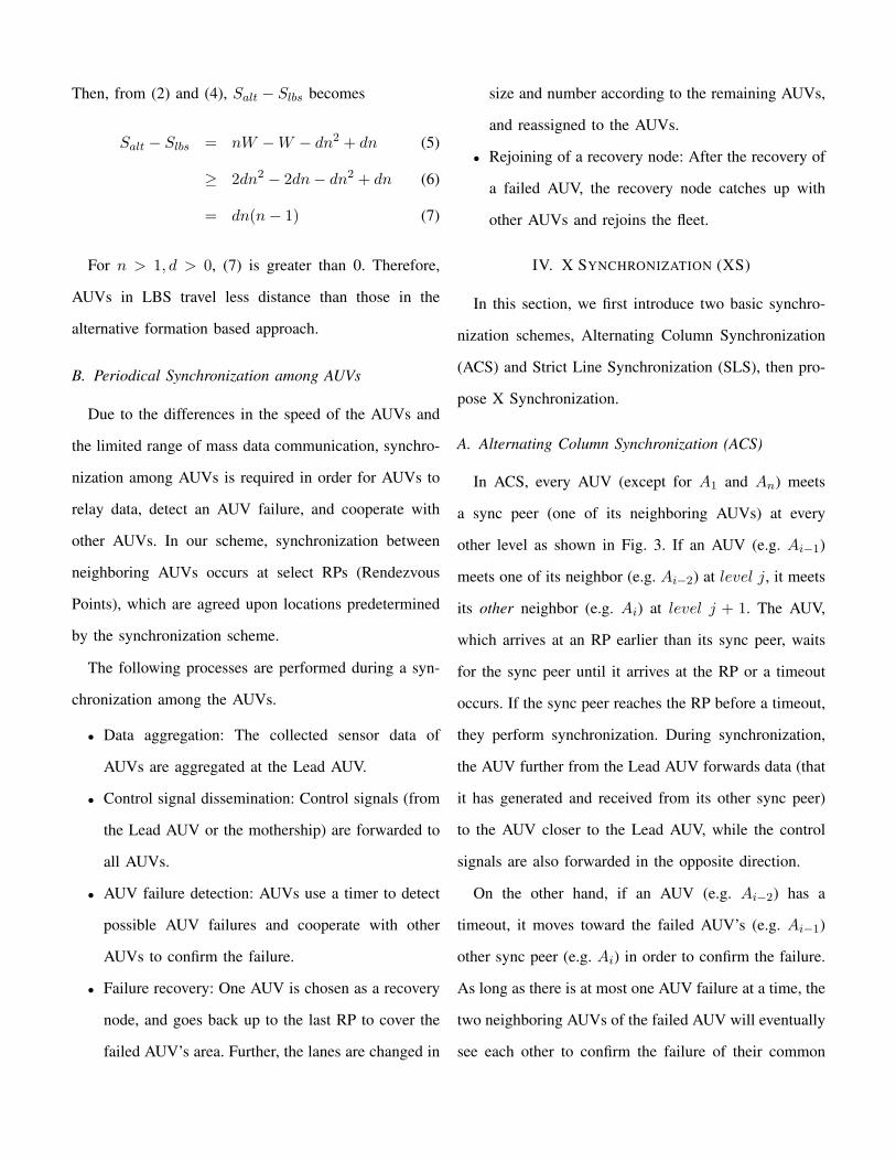
Then, from (2) and (4), Salt − Slbs becomes

Salt − Slbs = nW −W − dn2 + dn (5)

≥ 2dn2 − 2dn− dn2 + dn (6)

= dn(n− 1) (7)

For n > 1, d > 0, (7) is greater than 0. Therefore,

AUVs in LBS travel less distance than those in the

alternative formation based approach.

B. Periodical Synchronization among AUVs

Due to the differences in the speed of the AUVs and

the limited range of mass data communication, synchro-

nization among AUVs is required in order for AUVs to

relay data, detect an AUV failure, and cooperate with

other AUVs. In our scheme, synchronization between

neighboring AUVs occurs at select RPs (Rendezvous

Points), which are agreed upon locations predetermined

by the synchronization scheme.

The following processes are performed during a syn-

chronization among the AUVs.

• Data aggregation: The collected sensor data of

AUVs are aggregated at the Lead AUV.

• Control signal dissemination: Control signals (from

the Lead AUV or the mothership) are forwarded to

all AUVs.

• AUV failure detection: AUVs use a timer to detect

possible AUV failures and cooperate with other

AUVs to confirm the failure.

• Failure recovery: One AUV is chosen as a recovery

node, and goes back up to the last RP to cover the

failed AUV’s area. Further, the lanes are changed in

size and number according to the remaining AUVs,

and reassigned to the AUVs.

• Rejoining of a recovery node: After the recovery of

a failed AUV, the recovery node catches up with

other AUVs and rejoins the fleet.

IV. X SYNCHRONIZATION (XS)

In this section, we first introduce two basic synchro-

nization schemes, Alternating Column Synchronization

(ACS) and Strict Line Synchronization (SLS), then pro-

pose X Synchronization.

A. Alternating Column Synchronization (ACS)

In ACS, every AUV (except for A1 and An) meets

a sync peer (one of its neighboring AUVs) at every

other level as shown in Fig. 3. If an AUV (e.g. Ai−1)

meets one of its neighbor (e.g. Ai−2) at level j, it meets

its other neighbor (e.g. Ai) at level j + 1. The AUV,

which arrives at an RP earlier than its sync peer, waits

for the sync peer until it arrives at the RP or a timeout

occurs. If the sync peer reaches the RP before a timeout,

they perform synchronization. During synchronization,

the AUV further from the Lead AUV forwards data (that

it has generated and received from its other sync peer)

to the AUV closer to the Lead AUV, while the control

signals are also forwarded in the opposite direction.

On the other hand, if an AUV (e.g. Ai−2) has a

timeout, it moves toward the failed AUV’s (e.g. Ai−1)

other sync peer (e.g. Ai) in order to confirm the failure.

As long as there is at most one AUV failure at a time, the

two neighboring AUVs of the failed AUV will eventually

see each other to confirm the failure of their common

j

j + 1

j − 1

level

A1

Ai−2

lane1 · · · lanei−1 lanei lanei+1 lanen· · ·

Ai−1

Ai+1 AnAiAi−1

Ai−1Ai

Ai

Fig. 3. Alternating Column Synchronization

T.O.

T.O.

T.O.

waiting waiting

waiting

waiting waiting

waiting

waiting

waiting

(a)

(b)

(c)

(d)

(e)

(f)

lane1 lane2 lane3 lane4

level

2

1 4

1

1

1

1

1

2

2

2

2

2

4

4

4

4

4

j + 1

j

j + 1

j

j + 1

j

j + 1

j

j + 2

j + 1

j

j + 2

j + 1

j

j + 2

Fig. 4. Failure Detection and Recovery in ACS

neighbor. Note that to use ACS it is assumed that R ≥ h

and there is only one AUV failure at a time (XS and

SLS do not have these constraints). After the failure

confirmation, the AUV at a lower level (e.g. Ai−2) goes

back at most one level to cover the failed AUV’s area.

Afterwards, the AUV rejoins the other surviving AUVs,

and the fleet of AUVs continue the survey.

1) AUV Failure Detection and Recovery in ACS:

When Ak (1 < k < n) fails at an arbitrary level j,

both of its neighbors Ak−1 and Ak+1 (or sync peers) will

have a timeout at different moments at either level j and

level j +1 or level j +1 and level j respectively. As an

example in Fig. 4(a), A3 has failed, and A2 and A4 have

a timeout event in Fig. 4(b) and Fig. 4(c) respectively.

Immediately after having a timeout, neighboring nodes

of the failed AUV move to meet each other along the

cross line over the lane of the failed AUV up to a

distance of 2w. The maximum level difference between

the neighbors of the failed AUV is only 1, and hence the

AUV with an earlier timeout definitely meets the other

sync peer of the failed AUV within a distance of 2w.

If either one of those AUVs sees Ak while moving to

each other, the timeout event is false (they may have

had an inappropriate timeout period or Ak has traveled

with a much lower speed than expected). In that case,

they go back to their RP and wait for Ak for a normal

synchronization. If the two neighbors only see each other

(e.g., A2 and A4 as shown in Fig. 4(d)), they confirm

the failure of Ak (A3), and re-calculate the size of lanes

because there are only n − 1 active nodes. The AUV

which is at a lower level (A2 in Fig. 4(d)) is chosen as

a recovery node, and the recovery node covers the failed

AUV’s area at the current level. In this case, there is no

need for a recovery node to move levels back, because

level j−1 must have already been covered by the failed

AUV. The recovery node only needs to cover level j of

the failed AUV’s lane. The neighbors also forward the

information about the change of lanes and the failure to

other AUVs. In Fig. 4(f), there are only 3 lanes for 3

AUVs, and AUVs have new RPs represented as white

circles.

Note that if A1 (or An) fails, then A2 or (An−1) will

have a timeout event, and can immediately move towards

A3 (or An−2) to inform it and the rest of the AUVs of

the failure. Afterwards, A2 (or An−1) will go one level

below for recovery.

The frequent synchronization of ACS, and hence the

large aggregate synchronization delay over the operation

can degrade the performance in terms of the total search

time. However, ACS has a quick recovery process due

to the fact that a recovery node needs to go back to at

most one level for covering the area of failed AUV.

B. Strict Line Synchronization (SLS)

In SLS, synchronization among AUVs occurs at RPs

on designated sync lines. As shown in Fig. 5, the AUVs

have a sync line after every K levels during survey. The

AUVs first complete the survey in an area between two

consecutive sync lines, and then perform synchronization

before they continuing the survey. Every AUV (except

for A1 and An) has two RPs on a sync line as shown in

Fig. 5. An AUV first visits the RP further from the Lead

AUV in order to meet one of its sync peers. After the

AUV meets one of its sync peer (which is further from

the Lead AUV than the AUV itself) and receives data

from that sync peer, the AUV visits its other RP closer

to the Lead AUV to meet its other sync peer to forward

the data. Eventually, the data is aggregated at the Lead

AUV at the center of the fleet. Then, the control signal

from Lead AUV is disseminated to member AUVs in the

reverse order of sensor data aggregation.

If an AUV fails to reach a sync line, its two neighbors

will have a timeout and meet to confirm the failure. Then,

Section (K)

Sync lines

j + K

j

j + 2K

level

A1

Ai−1

Ai

Ai+1

An

lane1 · · · lanei−1 lanei lanei+1 lanen· · ·

Fig. 5. Strict Line Synchronization

one of them is chosen as a recovery node, and goes back

up to K levels to cover the failed AUV. Meanwhile,

the remaining AUVs adjust their lane assignment to

avoid any sensing coverage hole and continue the survey

operation. After finishing the recovery, the recovery node

will catch up with the other surviving AUV with a

straight line movement and join the fleet.

1) SLS algorithm at a sync line: The fleet is divided

into two groups: the left group and the right group. The

left group comprises AUVs that have IDs less than or

equal to dn+12 − 1e. Other AUVs belong to the right

group. Here n is the number of AUVs. There are two

center nodes in the middle of the fleet of AUVs, each

of which belongs to a different group. As shown in Fig.

6(a), there are only n− 1 RPs at a sync line.

Synchronization consists of two phases: the data ag-

gregation phase, and the control signal dissemination

phase. In the data aggregation phase, A1 moves to RP1,2

upon arrival at a sync line. For AUVs with ID greater

than 1 (i.e. i > 1), Ai moves to RPi−1,i (Here we

assume that Ai belongs to the left group.) If the AUV

belongs to the right group, it first moves to RPi,i+1,

and has the opposite moving direction. For example,

A2 first visits RP1,2 as shown Fig. 6(a). Note that, in

Fig. 6(a), all AUVs except A2 and A6 have already

arrived at the sync line. If RPi−1,i is already occupied

by Ai−1, then Ai receives data from Ai−1 and moves

to RPi,i+1. In other words, Ai−1 forces Ai to move

toward the center of the fleet (e.g., A1 and A2 force A2

and A3 to move toward the center as shown Fig. 6(b)

and Fig. 6(c) respectively). If RPi−1,i is not occupied,

Ai waits for Ai−1 until the timeout period expires or

Ai−1 arrives. In this way the two center nodes meet

at an RP eventually (e.g., A3 and A4 in Fig. 6(g)),

which means all AUVs, except for the nodes at the

edges, have met both of its neighbors and relayed data.

When the two center nodes meet at an RP, the Lead

AUV (which is one of the center nodes) receives data

of all AUVs and completes the data aggregation phase.

In the control signal dissemination phase that follows

the data aggregation phase, Ai receives a control signal

from Ai+1 at RPi,i+1, and moves toward RPi−1,i to

forward the signal. Immediately after forwarding the

control signal (without waiting for the completion of the

dissemination phase), Ai continues the search operation

up to the next sync line.

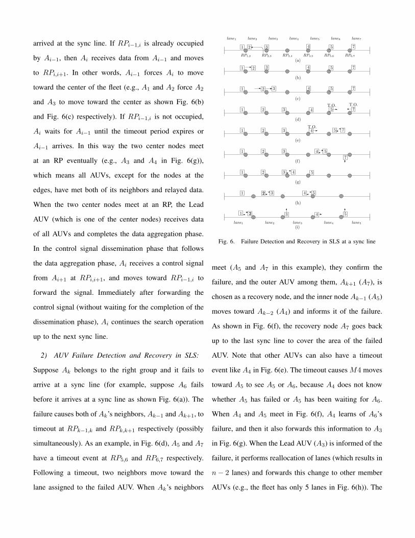
2) AUV Failure Detection and Recovery in SLS:

Suppose Ak belongs to the right group and it fails to

arrive at a sync line (for example, suppose A6 fails

before it arrives at a sync line as shown Fig. 6(a)). The

failure causes both of Ak’s neighbors, Ak−1 and Ak+1, to

timeout at RPk−1,k and RPk,k+1 respectively (possibly

simultaneously). As an example, in Fig. 6(d), A5 and A7

have a timeout event at RP5,6 and RP6,7 respectively.

Following a timeout, two neighbors move toward the

lane assigned to the failed AUV. When Ak’s neighbors

21 3

(h)

5 7

21 3 4 5 7

(b)

21 3 4 5 7

(c)

T.O.

T.O.

T.O.

21 3 4 5

(e)

21 3 4 5

7

(d)

(f)

21 3 4 52

(i)

21 3 4 52

lane1 lane2 lane3 lane4 lane5 lane6 lane7

lane1 lane2 lane3 lane4 lane5

21

(g)

5 7

RP1,2 RP2,3 RP3,4 RP4,5

(a)

5

RP5,6

7

RP6,7

1 2 3 4

3 4

4

Fig. 6. Failure Detection and Recovery in SLS at a sync line

meet (A5 and A7 in this example), they confirm the

failure, and the outer AUV among them, Ak+1 (A7), is

chosen as a recovery node, and the inner node Ak−1 (A5)

moves toward Ak−2 (A4) and informs it of the failure.

As shown in Fig. 6(f), the recovery node A7 goes back

up to the last sync line to cover the area of the failed

AUV. Note that other AUVs can also have a timeout

event like A4 in Fig. 6(e). The timeout causes M4 moves

toward A5 to see A5 or A6, because A4 does not know

whether A5 has failed or A5 has been waiting for A6.

When A4 and A5 meet in Fig. 6(f), A4 learns of A6’s

failure, and then it also forwards this information to A3

in Fig. 6(g). When the Lead AUV (A3) is informed of the

failure, it performs reallocation of lanes (which results in

n− 2 lanes) and forwards this change to other member

AUVs (e.g., the fleet has only 5 lanes in Fig. 6(h)). The

remaining n − 2 AUVs in the fleet do not wait for the

recovery node to return back to the sync line. Instead,

they continue the search operation. After the recovery

node finishes recovery, it catches up with the fleet with

linear movement and rejoins the fleet by sending a rejoin

request message to other AUVs. The rejoining process

occurs at a sync line where the recovery node arrives

earlier than other AUVs. After the recovery node rejoins

the fleet, the fleet of AUVs performs reallocation of lanes

and has n− 1 lanes. Note that the recovery node knows

the position of the Lead AUV, because the Lead AUV

periodically broadcasts control messages containing its

location with a high transmission power.

SLS may have a lower synchronization overhead than

ACS because, in SLS, the fleet of AUVs does not

synchronize at every level. This can reduce the total

search time. However, in SLS, it may take a longer time

to detect and recover from an AUV failure. Also note

that, unlike ACS in which only one AUV failure can be

handled at a time, SLS can handle multiple simultaneous

AUV failures, because, in SLS, all surviving AUVs are

on the same sync line during synchronization. In other

words, after having a timeout, each surviving AUV will

eventually meet its surviving neighbors on a sync line

by moving until it meets another AUV or reaches the

left border of the lane of A1 or the right border of the

lane of An.

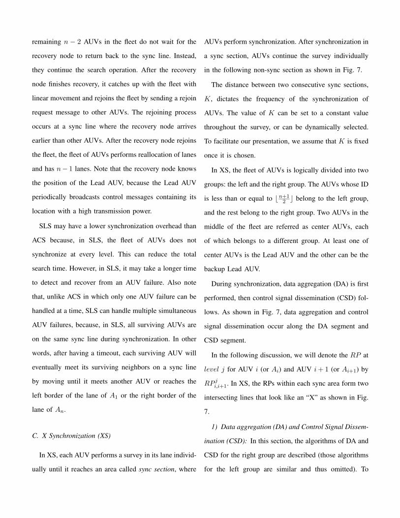
C. X Synchronization (XS)

In XS, each AUV performs a survey in its lane individ-

ually until it reaches an area called sync section, where

AUVs perform synchronization. After synchronization in

a sync section, AUVs continue the survey individually

in the following non-sync section as shown in Fig. 7.

The distance between two consecutive sync sections,

K, dictates the frequency of the synchronization of

AUVs. The value of K can be set to a constant value

throughout the survey, or can be dynamically selected.

To facilitate our presentation, we assume that K is fixed

once it is chosen.

In XS, the fleet of AUVs is logically divided into two

groups: the left and the right group. The AUVs whose ID

is less than or equal to bn+12 c belong to the left group,

and the rest belong to the right group. Two AUVs in the

middle of the fleet are referred as center AUVs, each

of which belongs to a different group. At least one of

center AUVs is the Lead AUV and the other can be the

backup Lead AUV.

During synchronization, data aggregation (DA) is first

performed, then control signal dissemination (CSD) fol-

lows. As shown in Fig. 7, data aggregation and control

signal dissemination occur along the DA segment and

CSD segment.

In the following discussion, we will denote the RP at

level j for AUV i (or Ai) and AUV i + 1 (or Ai+1) by

RP ji,i+1. In XS, the RPs within each sync area form two

intersecting lines that look like an “X” as shown in Fig.

7.

1) Data aggregation (DA) and Control Signal Dissem-

ination (CSD): In this section, the algorithms of DA and

CSD for the right group are described (those algorithms

for the left group are similar and thus omitted). To

Data Aggregation Point

Control Signal Dissemination Segment

Data Aggregation Segment

(Non-sync)

Data Flow

Control Signal Flow

level

j

j + n

j + n

2

j + n + K

j + 2n + K

Sync Section (n)

Section (K)

Surv

eydirectio

n

Sync Section (n)

Sync Section (n)Sync Section (n)

Fig. 7. X Synchronization

facilitate the presentations, we assume that the fleet has

n AUVs where n is an even number larger than 2. Fig.

8 illustrates the synchronization process and also shows

the flow of data and control signals.

Suppose that the sync section begins at level j as

shown in Fig. 8. The AUVs in the group use a slightly

different algorithm depending on their relative position

in the fleet as follows.

• Ai (where n2 + 1 < i < n): The AUV Ai surveys

its lane, lane i, until it reaches the RPn−i+ji,i+1 where

Ai is supposed to synchronize with Ai+1 at level

(n − i + j). At the RP, Ai receives the collected

sensor data from Ai+1 and appends its data to the

data. Then, as shown in Fig. 8, Ai moves to its next

RP at the level (n − i + j + 1), and forwards to

Ai−1 the aggregated data. Then, Ai continues the

survey up to RP i+j−1i−1,i to receive control signals

from Ai−1. Ai also forwards the control signal to

its other neighbor, Ai+1 at the next RP at level i+j,

before it continues the survey up to the next sync

section.

lanen

2+1 · · ·

lanei−1 lanei lanei+1 lanen· · ·

RPn−i+j

i,i+1

Ai−1

level

j

···

n − i + j

n − i + j + 1

···

n

2+ j

···

i + j − 1

i + j

n + j

···

RPn−i+j+1

i−1,i

···

···

RPn

2+j

n

2, n

2+1

RPi+j−1

i−1,i

RPi+j

i,i+1

Ai

Ai Ai+1

An

2+1

An

2

AiAi−1

Ai Ai+1

n − i + 1

2i − n + 1

n − i

···

···

Data

Contro

l Signa

l

An

An

j + 1

n + j − 1

RPj+1

n−1,n

Fig. 8. XS: Synchronization of the right group

• An: The rightmost AUV, An surveys its lane until

it reaches the RP where it synchronizes with An−1

at level j + 1. (denoted as RP j+1n−1,n in Fig. 8). At

the RP, An forwards data it has collected to An−1.

Then, An continues the survey up to its next RP at

level (n + j − 1) to synchronize with An−1 again

and receive control signals. After receiving control

signals, An continues the survey on its lane.

• An

2+1: A center AUV An

2+1 receives the data from

An

2+2 at the RP at level (n

2 +j−1). Then, it moves

to its next RP at the next level to synchronize with

the other center AUV, An

2. If An

2+1 the Lead AUV,

it receives the aggregated data of the left group, and

the DA phase is completed. An

2+1 communicates

with the mothership if necessary and then initiates

the CSD phase to disseminate the control signal or

commands.

2) AUV Failure Detection and Recovery: When Ai−1

has a timeout while waiting for Ai at an RP, it cooperates

with Ai+1 (the other neighbor of Ai) to confirm that

Ai has really failed. The failure confirmation process

is necessary, because the timeout at Ai−1 does not

necessarily indicate the failure of Ai; it is possible that

Ai has been waiting for Ai+1 at another RP. Following

the failure confirmation, an AUV is chosen as a recovery

node, and remaining AUVs adjust their lanes to cover the

survey region without any sensing coverage hole and to

re-balance the load.

Suppose Ai (n2 < i < n) fails before reaching a DA

segment in a sync section which begins at level j. The

failure of Ai leads to the timeouts of Ai−1 and Ai+1 at

RPn−i+ji−1,i and RPn−i+j+1

i,i+1 respectively. After having a

timeout, Ai−1 and Ai+1 move toward the lane of Ai as

shown in Fig. 9(a). If Ai−1 or Ai+1 can detect the signal

of Ai during their movement, the timeout is a false alarm

(which is possible due to a too small timeout value). In

such a case, Ai−1 and Ai+1 return to their RPs, and wait

for Ai for normal synchronization. If Ai−1 and Ai+1 see

each other but not Ai, as also shown in Fig. 9(a), they

confirm the failure of Ai and initiate a recovery process.

Here, for convenience, we assume that R, which is a

communication range of AUVs, is larger than the height

of a level (e.g. 2r). However, this constraint can be

readily removed by allowing AUVs to move along the

DA or CSD segment shown in Fig. 9.

After the failure confirmation, the AUV at a lower

level (Ai+1), becomes a recovery node as shown in Fig.

9(b), and goes back to cover the lane assigned to Ai up

to the previous DA segment. Meanwhile, the AUV at

a higher level, Ai−1, moves toward its other sync peer,

Ai−2, and informs Ai−2, which may or may not have

a timeout event, of the failure as also shown in Fig.

9(b), and continues the survey until it reaches the CSD

segment. The information about the failure is eventually

delivered to the Lead AUV at level (n2 +j). When receiv-

ing the failure information, the Lead AUV recalculates

the width and number of lanes based on remaining AUVs

and forwards a control signal containing this information

of new lanes to its neighbors. Ai−1 receives the control

signal at level i + j − 2 as shown in Fig. 9(c). To

deal with the fact that both Ai and Ai+1 are absent

from the CSD process, Ai−1 moves up and right towards

RP i+j+1i,i+1 to forward the control signal to Ai+2, which

may have a timeout and also been moving downward as

shown in Fig. 9(d). Then, Ai−1 moves toward its newly

assigned lane, and continues the survey up to the next

DA segment. After the recovery node (Ai+1) finishes

the recovery, it will catch up with other AUVs rejoin the

fleet in the first sync section encountered. Reallocation of

the lanes is similar to the failure detection and recovery

process.

If A1 or An fails, its neighbor (A2 or An−1) will

timeout at level j + 1. In this case, A2 (or An−1) does

not need failure confirmation, because it is not possible

that A1 or An is waiting for another AUV. Therefore, A2

(An−1) immediately moves toward its other neighbor,

A3 (An−2) to inform it of the failure. Then, A2 (An−1)

becomes a recovery node.

If a center AUV, An

2(or An

2+1) fails, An

2−1 and

An

2+1 (or An

2and An

2+2) have a timeout and meet to

confirm the failure. After confirmation of the failure,

the remaining center AUV forwards the control signal

i + j − 2

i + j − 1

i + j

i + j + 1

(a)

i i + 1i − 1i − 2

n − i + j

n − i + j + 1

n − i + j + 2

n − i + j − 1

(b)

level

Lane i i + 1i − 1i − 2

n − i + j

n − i + j + 1

n − i + j + 2

n − i + j − 1

(c)

level

Lane

(d)

Timeout

i i + 1i − 1i − 2

i + j − 2

i + j − 1

i + j

i + j + 1

i i + 1i − 1i − 2

Timeout

Ai+1

Ai−1

Ai+1

Ai−1

Ai−2

Ai−1 Ai+2

Lane Lane

level level

data data

control signalcontrol signal

Ai−2

Ai−1

Ai−2

Ai+2

Fig. 9. AUV failure detection and recovery

to An

2−2 and An

2+2 (or An

2−1 and An

2+3).

Note that the failure of one AUV can cause successive

timeouts. For example, during the DA phase, if Ai has

failed, all AUVs between An

2+1 and Ai−1 can have a

timeout event while waiting for their sync peer at right.

However, those cascaded timeouts will not cause any

problem. More specifically, when an AUV, Ak, where

n2 + 1 ≤ k < i− 1 has a timeout, it moves toward Ak+1

until it sees Ak+1 and it realizes that the timeout was a

false alarm and thus goes back to the normal state. Note

that Ak′ , where i + 2 ≤ k′ ≤ n, will not timeout as they

have already finished the synchronization for the current

DA phase.

So far, we have assumed that only one AUV failure

occurs at a time. However, XS can detect and recover

multiple simultaneous AUV failures. For example, in

Fig. 8, if two consecutive AUVs, Ai−1 and Ai, have

failed before they reach the DA segment, Ai−2 and

Ai+1 will have a timeout event, and they will meet

eventually while moving toward the lanes of Ai−1 and

Ai respectively along RPs on the DA segment. Note that

non-consecutive AUV failures can also be detected. For

example, in Fig. 8, if Ai−2 and Ai have failed, Ai−1 and

Ai+1 will first detect and confirm the failure of Ai, and

then, Ai−3 and Ai−1 will also detect and confirm the

failure of Ai−2 when they meet.

V. TIMEOUT CALCULATION

In this section, we derive the timeout values used

for failure detection in XS. A proper timeout period is

required to avoid either an unnecessary wait for a failed

AUV or a needless premature recovery process.

In XS, when Ai−1 and Ai synchronize at an RP, Ai−1

and Ai calculate the timeout value used at the next

RP where they will meet again. In order to determine

an appropriate timeout period for Ai−1 and Ai, the

distributions of the arrival time at the next RP of Ai−1

and Ai are estimated. Then, Ai−1 (Ai) chooses a timeout

period such that within that amount of time, Ai (Ai−1)

will arrive at the next RP with a high probability, say

Po, according to the estimated arrival time distribution.

The arrival time distribution of an AUV at an RP is

obtained using the estimated travel time distribution of

the AUV from the current RP to the next RP and the

delays introduced by synchronization among AUVs.

To facilitate the presentation, we first define a few

variables. Let random variable xi be the estimated arrival

time of Ai at the next RP, and let random variable tyi

be Ai’s travel time for a distance of y units. Also, let

dp,p+1 (1 ≤ p < n) represent the sync delay at an RP

which is the amount of time elapsed from the arrival of

the earlier AUV (between Ap or Ap+1) at the RP to the

completion time of the synchronization between Ap and

Ap+1.

Suppose that AUVs, Ai−1 and Ai, where bn+12 c+1 <

i ≤ n, synchronize with each other at an RP at level u

on a CSD segment as shown in Fig. 10. They calculate

the timeout period for each other for the next RP at level

(u+2(n−i+1)+K) at the next DA segment as follows.

The arrival time of Ai is estimated first. Between the

sync at RP ui−1,i and the next sync at RP

u+2(n−i+1)+Ki−1,i ,

three steps should occur in the same order as shown

in Fig. 10. First, the control signal is forwarded to An

at level (u + n − i) on the CSD segment. Then, An

performs survey up to its next RP at level (u + n− i +

K + 2). Finally, collected data are forwarded to Ai at

level (u+2(n− i)+K +1), and then, Ai moves toward

to RPu+2(n−i+1)+Ki−1,i to forward data to Ai−1. Therefore,

the arrival time of Ai is the sum of the time needed to

complete these steps.

In both the CSD and DA phases, the data or control

signals are forwarded through 2(n − i) RPs, and the

distance between two RPs is w + h. Also suppose

the synchronization at RP ui−1,i occurs at time 0. Let a

random variable xi be the arrival time of Ai at the RP at

level u+2(n− i+1)+K. Then, xi can be represented

as

xi = t(w+h)i + · · ·+ t(w+h)

n−1 + t(w+h)n−1 + · · ·+ t(w+h)

i (8)

+ t(w+h)(K+2)n (9)

+ di,i+1 + · · ·+ dn−1,n + dn,n−1 + · · ·+ di+1,i (10)

where the first line represents the sum of travel time of

Aj (i ≤ j ≤ n−1) during DA and CSD, and the second

line represents the survey time of An for K + 2 levels,

and the third line represents the sum of sync delay among

AUVs during DA and CSD.

Assume that the speeds and corresponding travel times

of all AUVs have the same statistical properties i.e.,

t(w+h)p = t(w+h)

p+1 (where 1 ≤ p < n). In addition, we

observe that, when Aj (i ≤ j ≤ n) arrives at RPj−1,j

on the DA segment, most probably Aj−1 has already

arrived at the RP. This is because, for Aj to arrive at the

RP, as many as 2(n− j) synchronization should precede

at other RPs, while the arrival of Aj−1 does not require

any preceding synchronization (and Aj and Aj−1 have an

equal distance to travel). For the same reason, when Aj′

(i ≤ j′ < n) arrives at RPj′,j′+1 on the CSD segment,

most probably Aj′+1 has already arrived at the RP.

Under these observations, we assume that an AUV (the

left-hand side AUV during CSD and the right-hand side

AUV during DA) can begin synchronization immediately

after it arrives at an RP without waiting for its sync peer.

Also, for simplicity, the time to transmit data and control

signals between two sync peers is assumed to be some

constant value dsync. From the above observations and

assumptions, we have dp,p+1 = dsync where 1 ≤ p < n.

Then, (8) through (10) can be simplified into

xi = t(K+2n−2i+2)(w+h) + 2dsync(n− i) (11)

On the other hand, xi−1, the arrival time of Ai−1, can

be directly obtained from the travel time distribution of

an AUV, because no synchronization is required for Ai−1

to arrive at the next RPu+2(n−i+1)+Ki−1,i . Therefore, xi−1

lanei−1 lanei lanei+1 · · · lanen

levelu + 2(n − i + 1) + K

u

· · ·

· ··

···

··· K

DA Segment

CSD Segment

Sync section l + 1

Sync section lAi−1 Ai

Ai−1 Ai

Ai+1

An

Ai+1

u + n − i + K + 2

u + n − i

Fig. 10. Illustration for timeout period calculation for the right group

becomes

xi−1 = t(w+h)(2(n−i+1)+K) (12)

Let x′ be the random variable representing the arrival

time of an AUV at an RP on the CSD segment. x′ can

also be obtained in a similar way that x is obtained, and

hence, the discussion is omitted.

Now, we discuss the estimation of the travel time

distribution that is used in (11) and (12). Recall that

a random variable ty represents the travel time of an

AUV for a distance y. In order to estimate the travel

time distribution of an AUV for a given distance y (e.g.

between two consecutive RPs of the two AUVs), we

first obtain the travel time distribution of an AUV for

a distance d for some value d (which is much less than

w) through simulations. More specifically, Let random

variable s be the travel time of an AUV for a distance d,

and the probability density function (pdf) of s be given

as fs(s). Let m = yd , then ty can be represented as the

sum of s.

ty = s1 + s2 + · · ·+ sm (13)

Because si is i.i.d., the pdf of ty is the convolution

of fsi(ty) where 1 ≤ i ≤ m. Further, according to the

0

0.02

0.04

0.06

0.08

0.1

1200 1250 1300 1350 1400 1450 1500 1550 1600

Prob

abili

ty

Arrival time

Actual arrivalEstimated arrival

Fig. 11. Distribution of actual and estimated arrival of an AUV

Central Limit Theorem, the distribution of ty approaches

a normal distribution if m is large enough. Specifically,

let µ and σ2 represent the mean and variance of s

respectively, then ty will approximately follow a normal

distribution with the mean, mµ, and the variance, mσ2.

Let D be the total synchronization delay, then, the

estimated arrival time xi also follows a normal distribu-

tion with (mµ+D, mσ2) as its mean and variance. From

the distribution function of xi, an arrival time, t0, that

corresponds to a given probability P0 is chosen as the

candidate of the timeout period (i.e. P [x ≤ t0] = P0).

Fig. 11 shows the probability distribution of the actual

and estimated arrival time of an arbitrary AUV at its RPs

during survey with a sample value of the lane width and

K (w = 550m, K=53). The pdf of the actual arrival

time was obtained through simulations. Fig. 11 shows

that the actual arrival time of the AUV approximately

follows a normal distribution. The timeout value, TO is

chosen as TO = βt0 where β is a design parameter to

add some safety margin to reduce premature timeouts.

VI. NUMERICAL ANALYSIS

In this section, we discuss a mathematical models

to approximate the total survey completion time and

traveling distance of AUVs using XS, which will be

verified through simulations in the next section. Both

AUV failure and non-failure cases will be considered.

Let d-section (or diamond section) be defined to be

the area between two consecutive DA points (e.g. the

area between level k and level k+n+K shown in Fig.

12).

The expected survey time for a d-section is first calcu-

lated and used in order to obtain the total survey time for

the entire area. The effect of R will be also considered

for more accurate approximation of the survey time.

A. The Case with No AUV Failure

1) Total Survey Time: Suppose two center AUVs meet

at a DA point at level k, and complete the current DA

phase as shown in Fig.12. From this moment to the

completion of the next DA phase, three steps should

be completed by both the left and the right groups.

First, the control signal is forwarded to the A1 (or An)

at level (k + n2 − 1). Then, A1 (or An) performs the

survey operation until it reaches its next RP at level

(k + n2 + K + 1). Finally, data is forwarded to the

center AUVs, which meet at the next DA point at level

(k + n + K). Therefore, the survey time for a d-section

will be the arrival time (at the next DA point) of the

slowest center AUV between two center AUVs, after the

completion of the CSD phase, the survey of K levels by

A1 (or An), and the DA phase.

During the CSD phase and the DA phase, the data

or the control signals are forwarded through n− 2 RPs.

The distance between two RPs is w + h, and all AUVs,

except A1 and An, need to move a distance of w +

h − R to communicate with its sync peer. Therefore,

the total travel distance of AUVs for CSD and DA is

(n − 2)(w + h − R). Afterward, A1 (or An) travels a

distance of (K + 2)(w + h) − R. Let P be the sum of

the travel distance for CSD, DA, and the survey of A1

(or An) in a d-section. Then, P is

P = (n− 2)(w + h−R) + (K + 2)(w + h)−R (14)

Let random variable u be an AUV’s travel time for

the distance of P . u can be represented as the sum of s

in a similar way to (13). Also let v be the arrival time

of a center AUV at the next DA point. Then, v is

v = u + dsync × (n− 2) (15)

Also let y be the arrival time of the slowest center

AUV between the two center AUVs. Then, we have,

y = max(v,v) (16)

Note that the pdf of v, fv(v), can be obtained from

the pdf of u and (15). From fv(v), the probability

distribution function, Fv(v) can also be obtained. Let

fy(y) be the pdf of y. Then, from (16), accounting for

the fact that we are taking the maximum of two random

variables v’s, we have

fy(y) = 2Fv(y)fv(y) (17)

Let C = 1√2πmσ2

, then the expected arrival time of

n + K

Level

k

k + n + K

k +n

2+ K

k +n

2

Fig. 12. Calculation of the survey time in a d-section

the slowest center AUV is

E[y] =∫ ∞

−∞yfy(y)dy (18)

= 2∫ ∞

−∞yFv(y)fv(y)dy (19)

= 2C2

∫ ∞

−∞y(

∫ y

−∞e−

(x−mµ)2

2mσ2 dx)e−(y−mµ)2

2mσ2 dy(20)

The two center AUVs also need the time dsync to

exchange data. Therefore, the expected survey time for a

d-section is E[y]+dsync. The expected total survey time,

TXS , is the product of the survey time for a d-section

and the total number of d-sections, that is,

TXS = (E[y] + dsync)× L

n + K(21)

2) Average Travel Distance of AUVs: We first cal-

culate the total travel distance of the AUVs to obtain

the average travel distance of AUVs. At every level, the

distance for all AUVs to travel for the horizontal survey

is w×n. To move to the next level, each AUV moves a

distance of h. Thus, the total travel distance of AUVs is

wnL+h(L−1)n. Therefore, the average travel distance

of AUVs, SXS is

SXS = L(w + h)− h (22)

B. The Case with an AUV failure

1) Total Survey Time: Suppose one AUV fails at an

arbitrary level f . During the recovery, n − 2 AUVs

perform the survey. After the recovery node rejoins the

fleet, n − 1 AUVs perform the survey. Therefore, the

entire area can be logically partitioned into three zones

according to the number of AUVs performing the survey.

Let Zone A, Zone B, Zone C be the sub-areas which

are surveyed by n, n− 2, and n− 1 AUVs respectively.

Then, there are two cases to be considered for calculation

of the total survey time.

• Case 1: After the recovery node rejoins the fleet of

AUVs, the fleet completes the survey;

• Case 2: Before the recovery node rejoins the fleet

of AUVs, other AUVs reach the end of the survey

area;

In this paper, Case 1, the general case, will be dis-

cussed. Case 2 can be readily extended from Case 1,

and thus will be omitted.

Let random variable T i represent the survey time for a

d-section with i AUVs, and Df be the time elapsed from

the arrival of the fleet at a DA segment to the detection

of the failure. Also, let p, q be the number of d-sections

in Zone A and Zone B respectively. Let the total survey

time for the entire area with a failure at level f be Tf .

We assume that the area of interest has exactly g number

of d-sections for simplicity. Then Tf becomes

Tf = pTn + qTn−2 + (g − p− q)Tn−1 + Df (23)

Thus, the expected survey time is

E[Tf ] = pE[Tn]+qE[Tn−2]+(g−p−q)E[Tn−1]+E[Df ]

(24)

Note that p = min(p : p × (n + K) ≥ f) where

p ∈ N. The value of q depends on when the recovery

node rejoins other AUVs. For simplicity, we assume that

both failure detection and reallocation of lanes occur at

the same level of DA point. Then, the recovery node

moves a distance of (K+n)h to go back to the last sync

section. Then, to cover the lane of the failed AUV up to

the current DA point, it moves a distance of (K+n)(w+

h). Finally, it moves in a straight line for a distance of

qh(K +n−2) to catch up with other AUVs. Let random

variable Rt be the time taken for the recovery node to

move a distance of (K + n)h + (K + n)(w + h) and

E[Rt] be the expected value of Rt. Also let Rf be the

time needed for the recovery node to move a distance of

h(K + n− 2). Then, q can be approximated as follows.

q = min(q : q × E[Tn−2] ≥ E[Rt] + qE[Rf ]) (25)

= min

(q : q ≥ E[Rt]

E[Tn−2]− E[Rf ]

)(26)

Note that E[Tn], E[Tn−1], and E[Tn−2] can be

obtained using (25). The pdfs of Rt and Rf are obtained

in a similar way to (13). Then, E[Rt] and E[Rf ] are

calculated based on their pdf. To approximate Df , we

simply subtract the expected survey time of the fleet in

a section from the average timeout period of AUVs, i.e.,

E[Df ] ≈Pn

i=1 TOi

n −E[Tn].

With these obtained values, the expected survey time

of the fleet with a failure at level f can be calculated

from (24).

Finally, the failure can occur at any level between

level 1 and level L with a uniform probability. Then,

the expected survey time with a failure at an arbitrary

level, TXS becomes

TXS =L∑

f=1

E[Tf ]L

(27)

2) Average Travel Distance of AUVs: We first calcu-

late the total distance of AUVs. Let Si be the total travel

distance of the fleet with i AUVs to survey a d-section.

Then, we have

Si = i× (K + i)× (w + h) (28)

Let IA, IB , and IC be the total travel distance of AUVs

to survey Zone A, Zone B, Zone C respectively. An

AUV fails at level f in Zone A. Therefore, IA is

IA = np(K + n)(w + h)− (p(K + n)− f)(w + h) (29)

= (w + h)(p(K + n)(n− 1) + f) (30)

In Zone B, the fleet performs the survey with n − 2

AUVs. Therefore,

IB = q(n− 2)(K + n− 2)(wn

n− 2+ h) (31)

where q can be obtained using (26).

Similarly, the distance for the survey of zone C is

IC = (g − p− q)(n− 1)(K + n− 1)(wn

n− 1+ h) (32)

Let IR be the distance the recovery AUV moves for

the recovery and rejoining the fleet. Then, we have

IR = (w + h)(K + n) + h(K + n) + qh(K + n) (33)

= (K + n)(w + h(2 + q)) (34)

Then, the total travel distance of AUVs with a failure

at level f , Sf is the sum of IA, IB , and IC . That is,

Sf = IA + IB + IC + IR (35)

The expected distance of AUVs with a failure at an

arbitrary level, SXS , becomes

SXS =1

nL

L∑

f=1

Sf (36)

VII. PERFORMANCE STUDY

In this section, we present simulation results to com-

pare the performance of XS with two other synchroniza-

tion schemes, ACS and SLS.

The survey completion time and the travel distance

of AUVs for surveying a rectangular area (e.g. one

survey region shown in Fig. 2) have been chosen as

the performance metrics. The fleet of 12 AUVs perform

survey in an area of 80km2 (10km × 8km). According

to LBS, each AUV is initially responsible for a lane

of 1000012 m × 8000m. The swath width of each AUV

is set to 20m, which results in L = 400 levels. The

data transmission range of AUVs is set to be 20m.

The Discrete Gauss-Markov process model [32] is used

to emulate the practical speed variation of AUVs. The

initial speed and the memory level are set to 3m/s

and 0.5 respectively (memory level of 0.0 represents a

random walk mobility pattern and memory level of 1.0

results in a constant velocity fluid-flow model). Timeout

periods for detection of an AUV failure are calculated

with the parameters Po = 0.999.

Intuitively, XS should outperform the ACS and SLS.

ACS introduces a large overall synchronization overhead

due to its frequent synchronization as each AUV needs

to synchronize with one of its neighbors at every level.

Also, an AUV in SLS has to stay at a sync line until

all AUVs forward data to the Lead AUV and the AUV

receives the control signal from the Lead AUV, which

leads to a large sync delay, especially with a small value

of K. Further, SLS requires dedicated horizontal moves

of AUVs for synchronization on a sync line.

In Fig. 13 and Fig. 14, the Y axis represents the

normalized survey time and the travel distance of AUVs,

when the corresponding simulation results for ACS are

set to 1. The X axis represents the ratio of K to L,

denoted by u. Recall that K determines how often

the AUVs in SLS or XS perform synchronization. For

example, u = 1 (or K = L) means there is no

synchronization during survey. Note that u does not

affect the performance of ACS. Fig. 13 and Fig. 14

also show how closely the numerical estimation of the

performance approximates the simulation results.

Fig. 13 compares the performance of the schemes with

no AUV failure. As shown in Fig. 13(a), the survey time

of XS is always lower than that of ACS or SLS due to

the fact that XS introduces less synchronization. As u

grows, the survey time of both XS and SLS decreases

because a large value of u (or K) represents infrequent

synchronization which results in less synchronization

0.6

0.7

0.8

0.9

1

1.1

1.2

1.3

1.4

0 0.1 0.2 0.3 0.4 0.5 0.6 0.7

Nor

mal

ized

Sea

rch

Tim

e

u = K / L

ACS SimACS Anal

SLS SimSLS Anal

XS SimXS Anal

(a) Survey Time

0.7

0.8

0.9

1

1.1

1.2

1.3

1.4

0 0.1 0.2 0.3 0.4 0.5 0.6 0.7

Nor

mal

ized

Dis

tanc

e

u = K / L

ACS SimACS Anal

SLS SimSLS Anal

XS SimXS Anal

(b) Distance

Fig. 13. Varying size of K without a AUV failure

0.6

0.8

1

1.2

1.4

1.6

0 0.1 0.2 0.3 0.4 0.5 0.6 0.7

Nor

mal

ized

Sea

rch

Tim

e

u = K / L

ACS SimACS Anal

SLS SimSLS Anal

XS SimXS Anal

(a) Survey Time

0.7

0.8

0.9

1

1.1

1.2

1.3

1.4

0 0.1 0.2 0.3 0.4 0.5 0.6 0.7

Nor

mal

ized

Dis

tanc

e

u = K / L

ACS SimACS Anal

SLS SimSLS Anal

XS SimXS Anal

(b) Distance

Fig. 14. Varying size of K with a AUV failure

overhead, which is a positive effect on the survey time.

When there is no AUV failure, the travel distance

of ACS is equal to that of XS as shown in Fig. 13(b)

because the AUVs in ACS or XS follow the exactly same

path determined by the LBS described in Section III. The

distance of SLS is larger than that of ACS or XS due to

extra movements for synchronization on sync lines. Note

that XS does not require dedicated horizontal moves by

AUVs for synchronization as SLS does.

Fig. 14 shows the results with an AUV failure. An

AUV is set to fail at an arbitrary level. As shown in Fig.

14(a), the survey time of XS decreases as u grows until

u reaches about 0.2. As u grows beyond 0.2, however,

the survey time of XS increases, and eventually becomes

larger than that of ACS. This comes from the fact that a

large value of u (or K) has negative effects on the survey

time unlike in the case of no AUV failure. Suppose that

an AUV fails at an arbitrary position. A large value of K

causes a large amount of time for the recovery node to

go back to the last RP and survey. Thus, the fleet has to

survey with only (n− 2) AUVs for a long time until the

recovery node rejoins. Further, it is possible that other

AUVs arrive at the end of the survey area before the

recovery AUV rejoins. In this case, the survey will not

be completed until the recovery AUV arrives at the end

of the survey area. Due to both the negative and positive

effects of K, there is an optimal value of K which results

in the minimum survey time.

As shown in Fig. 14(b), SLS has the largest average

distance. XS and ACS have almost same travel distance

when the value of u is small. Note that the travel distance

of XS increases as u grows. The difference between the

travel distances of XS and ACS, however, is less than

5% of the travel distance of ACS even in the case of a

large value of u.

VIII. CONCLUDING REMARKS

The work represents the first attempt to the design and

qualitative as well as quantitative analysis of search and

survey algorithms using cooperative AUVs with failure

tolerance.

In this paper, we have proposed a rendezvous algo-

rithm, X Synchronization, for cooperative search and

survey using a fleet of AUVs with limited energy and

communication capabilities. XS enables AUVs to survey

a large area for time-sensitive applications tolerating

AUV failures via mobility-assisted data communication.

We have derived appropriate synchronization timeout

periods to reduce the number of false alarms by estimat-

ing the arrival time of AUVs. A numerical model has

also been devised to approximate the survey time and

traveling distance of AUVs. Results from simulations

and numerical analysis show that XS can outperform two

other rendezvous algorithms (ACS and SLS) in terms of

the total survey time and the travel distance of AUVs.

IX. ACKNOWLEDGEMENT

The authors would like to thank Bill Collins of Quester

Tangent Corp. for his useful suggestions.

REFERENCES

[1] B. Jalving, G. K., H. O. K., and V. K., “A toolbox of aiding

techniques for the HUGIN AUV integrated inertial navigation

system,” in Oceans, Piscataway, NJ, 2003.

[2] J. Heidemann, W. Ye, J. Wills, A. Syed, and Y. Li, “Research

challenges and applications for underwater sensor networking,”

in Proceedings of the IEEE Wireless Communications and

Networking Conference. Las Vegas, Nevada, USA: IEEE, April

2006, pp. 228–235.

[3] T. M. Ian F. Akyildiz, D. Pompili, “Underwater acoustic sensor

networks: Research challenges,” Ad Hoc Networks (Elsevier),

vol. 3, pp. 257–279, 2005.

[4] E. Sozer, M. Stojanovic, and J. Proakis, “Underwater acoustic

networks,” IEEE Journal of Oceanic Engineering, vol. 25, no. 1,

pp. 72–83, 2000.

[5] J. W. Bales and C. Chryssostomidis, “High bandwidth, low-

power,short-range optical communication underwater,” in Pro-

ceedings of 9th Internationa Symposium on Unmanned Unteth-

ered Submersible Technology, 1995.

[6] J. Delaney, A. Chave, G. R. Heath, B. Howe, and P. Beauchamp,

“Neptune: real-time, long-term ocean and earth studies at the

scale of a tectonic plate,” in OCEANS, MTS/IEEE Conference

and Exhibition, vol. 3, Honolulu, HI, USA, 2001, pp. 1366–

1373.

[7] R. A. Stephen, “Ocean seismic network seafloor observatories,”

Oceanus, pp. 33–37, March 1998.

[8] M. Grasmueck, G. P. Eberli, D. A. Viggiano, T. Correa,

G. Rathwell, and J. Luo, “Autonomous underwater vehicle

(AUV) mapping reveals coral mound distribution, morphology,

and oceanography in deep water of the straits of florida,”

GEOPHYSICAL RESEARCH LETTERS, vol. 33, 2006.

[9] D. R. Yoerger, M.Jakuba, A. M. Bradley, and B. Bing-

ham, “Techniques for deep sea near bottom survey using

an autonomous underwater vehicle,” International Journal of

Robotics Research archive, vol. 26, pp. 41,54, October 2007.

[10] D. Fornari, M. Tivey, H. Schouten, M. Perfit, K. V. Damm,

D. Yoerger, A. Bradley, M. Edwards, R. Haymon, T. Shank,

D. Scheirer, and P.Johnson, “Submarine lava flow emplace-

ment processes at the east pacific rise 9 50’n: Implications

for hydrothermal fluid circulation in the upper ocean crust,”

The Thermal Structure of the Ocean Crust and Dynamics of

Hydrothermal Circulation, vol. 148, 2004.

[11] M.-H. Cormier, W. B. Ryan, A. M. Bradley, D. R. Yoerger,

A. Shah, J. Sinton, R. Batiza, and K. Rubin, “Variable extrusive

emplacement mechanisms in the axial region of the east pacific

rise,” Geology, vol. 31, no. 7, 2003.

[12] E. Fiorelli, N. Leonard, P. Bhatta, D. Paley, R. Bachmayer, and

D. Fratantoni, “Multi-AUV control and adaptive sampling in

Monterey bay,” in Proceedings of IEEE Autonomous Underwa-

ter Vehicles: Workshop on Multiple AUV Operations (AUV04),

June 2004.

[13] J. Catipovic, D. Brady, and S. Etchemendy, “Development of

underwater acoustic modems and networks,” Oceanography,

vol. 6, pp. 112–119, 1993.

[14] M. Stojanovic, “Recent advances in high-speed underwater

acoustic communications,” IEEE Journal of Oceanic Engineer-

ing, vol. 21, pp. 125–136, 1996.

[15] L. Freitag, M. Stojanovic, M. Grund, and S. Singh, “Acous-

tic communications for regional undersea observatories,” in

Oceanology International, London, U.K, 2002.

[16] N. Farr, A. Chave, L. Freitag, J. Preisig, S. White, D. Yoerger,

and F. Sonnichsen, “Optical modem technology for seafloor

observatories,” in Proceedings of IEEE OCEANS, September

2006, pp. 1–6.

[17] J. Joe and S. H. Toh, “Digital underwater communication using

electric current method,” OCEANS 2007, pp. 1–4, 2007.

[18] G. Wang, G. Cao, and T. L. Porta, “Movement-assisted sensor

deployment,” in IEEE INFOCOM Conference Proceedings,

March 2004.

[19] J. Wu and S. Yang, “Smart: A scan-based movement-assisted

sensor deployment method in wireless sensor networks,” in

IEEE INFOCOM Conference Proceedings, March 2005.

[20] B. Liu, P. B. O. Dousse, P. Nain, and D. Towsley, “Mobility

improves coverage of sensor networks,” in ACM MobiHoc,

2005.

[21] A. Khan, C. Qiao, and S. K. Tripathi, “A failure-tolerant mobile

traversal scheme based on triangulation coverage,” in Proceed-

ings of International Conference on Heterogeneous Networking

for Quality, Reliability, Security and Robustness (Qshine) and

ICC 2007, Vancouver, Canada, August 2007.

[22] (2005, August) Abe: The autonomous benthic explorer.

[Online]. Available: http://www.whoi.edu/sbl/liteSite.do? lite-

siteid=4050&articleId=6343

[23] (2005, October) Unmanned aircraft sys-

tems roadmap 2005-2030. [Online]. Available:

http://www.fas.org/irp/program/collect/ uav roadmap2005.pdf

[24] R. Behringer, W. Travis, R. Daily, D. Bevly, W. Kubinger, and

W. H. V. Fehlberg, “Rascal - an autonomous ground vehicle for

desert driving in the darpa grand challenge 2005,” in Poceedings

of IEEE Intelligent Transportation Systems, September 2005,

pp. 644–649.

[25] C. W. Reynolds, “Flocks, herds, and schools: a distributed

behavioral model,” Computer Graphics, vol. 21, no. 6, pp. 25–

34, July 1987.

[26] T. Vicsek, A. Czirok, E. B. Jacob, I. Cohen, and O. Schochet,

“Novel type of phase transitions in a system of self-driven

particles,” Physical Review Letters, vol. 75, pp. 1226 – 1229,

1995.

[27] A. Jadbabaie, J. Lin, and A. S. Morse, “Coordination of groups

of mobile autonomous agents using nearest neighbor rules,”

IEEE Transactions on Automatic Control, vol. 48, pp. 988 –

1001, June 2003.

[28] X. Cui, T. Hardin, R. K. Ragade, , and A. S. Elmaghraby,

“A swarm-based fuzzy logic control mobile sensor network

for hazardous contaminants localization,” in The IEEE Interna-

tional Conference on Mobile Ad-hoc and Sensor Systems (MASS

2004), FortLauderdale, Florida, U.S.

[29] D. Payton, M. Daily, R. Estowski, M. Howard, and C. Lee,

“Pheromone robotics,” Autonomous Robots, vol. 11, no. 3, pp.

319–324, November 2001.

[30] P. E. Rybski, S. Stoeter, M. D. Erickson, M. L. Gini, D. F.

Hougen, and N. Papanikolopoulos, “A team of robotic agents

for surveillance,” in Fourth International Conference on Au-

tonomous Agents (Agents 2000).

[31] Image of mid-atlantic ridge. [Online]. Available:

http://www.ngdc.noaa.gov/

[32] B. Liang and Z. J. Haas, “Predictive distance-based mobility

management for multidimensional pcs networks,” IEEE/ACM

Transcations on Networking, vol. 11, no. 5, pp. 718 – 732,

October 2003.