model predictive control for autonomous and cooperative
TRANSCRIPT

HAL Id: tel-01635261https://pastel.archives-ouvertes.fr/tel-01635261
Submitted on 14 Nov 2017
HAL is a multi-disciplinary open accessarchive for the deposit and dissemination of sci-entific research documents, whether they are pub-lished or not. The documents may come fromteaching and research institutions in France orabroad, or from public or private research centers.
L’archive ouverte pluridisciplinaire HAL, estdestinée au dépôt et à la diffusion de documentsscientifiques de niveau recherche, publiés ou non,émanant des établissements d’enseignement et derecherche français ou étrangers, des laboratoirespublics ou privés.
Model predictive control for autonomous andcooperative driving
Xiangjun Qian
To cite this version:Xiangjun Qian. Model predictive control for autonomous and cooperative driving. Automatic Con-trol Engineering. Université Paris sciences et lettres, 2016. English. �NNT : 2016PSLEM037�. �tel-01635261�

THÈSE DE DOCTORAT
de l’Université de recherche Paris Sciences et Lettres PSL Research University
Préparée à MINES ParisTech
Commande Prédictive pour Conduite Autonome et Coopérative
Model Predictive Control for Autonomous and Cooperative Driving
COMPOSITION DU JURY :
M. Denis Gillet Ecole Polytechnique Fédérale de Lausanne, Rapporteur
M. Sébastien Glaser IFSTTAR, Rapporteur
M. Philippe Martinet Ecole Centrale de Nantes, Président
M. Christoph Stiller Karlsruhe Institute of Technology, Membre du jury
M. Arnaud de La Fortelle MINES ParisTech, Membre du jury
M. Fabien Moutarde MINES ParisTech, Membre du jury
Soutenue par Xiangjun Qian le 15 Décembre 2016 h
Ecole doctorale n°432
SCIENCES DES METIERS DE L’INGENIEUR
Spécialité Informatique temps-réel, robotique et automatique
Dirigée par Arnaud de La Fortelle Fabien Moutarde
h


Abstract
Autonomous driving has been gaining more and more attention in the last decades,
thanks to its positive social-economic impacts including the enhancement of traf-
�c e�ciency and the reduction of road accidents. A number of research institutes
and companies have tested autonomous vehicles in tra�c, accumulating tens of
millions of kilometers traveled in autonomous driving. With the vision of massive
deployment of autonomous vehicles, researchers have also started to envision coop-
erative strategies among autonomous vehicles. This thesis deals with the control
architecture design of individual autonomous vehicles and cooperative autonomous
vehicles. Model Predictive Control (MPC), thanks to its e�ciency and versatility,
is chosen as the building block for various control architectures proposed in this
thesis. In more detail, this thesis �rst presents a classical hierarchical control archi-
tecture for individual vehicle control that decomposes the controller into a motion
planner and a tracking controller, both using nonlinear MPC. In a second step, we
analyze the inability of the proposed planner in handling logical constraints raised
from tra�c rules and multiple maneuver variants, and propose a hybrid MPC based
motion planner that solves this issue. We then consider the convoy control prob-
lem of autonomous vehicles in which multiple vehicles maintain a formation during
autonomous driving. A hierarchical formation control architecture is proposed com-
posing of a convoy supervisor and local MPC based vehicle controllers. Finally, we
consider the problem of coordinating a group of autonomous vehicles at an intersec-
tion without tra�c lights. A hierarchical architecture composed of an intersection
controller and multiple local vehicle controllers is proposed to allow vehicles to cross
the intersection smoothly and safely.
Keywords: autonomous driving, cooperative autonomous driving, model predic-
tive control, hybrid model predictive control, motion planning, formation control,
autonomous intersection management


Acknowledgment
My profound gratitudes �rst go to my directors of thesis: Arnaud de La Fortelle
- who hired me even though I had just quited an unsuccessful Ph.D. thesis and
supported me to pursuit what I was interested in, and Fabien Moutarde - who un-
conditionally helped me when I was in di�cult situation and was always supportive
when I made decisions on the research directions. Your guidance was indispensable
for the achievement of this thesis.
The thesis could not be �nished without the immense love of my family: my wife
Ning Tan, my parents Lihong Zhu and Qiwei Qian, and my grandparents Juying Liu
and Xuexing Qian. You accompanied and will accompany me for ups and downs
and you are my reasons to keep moving forward.
Paris is a great city for living and research, but it is always bene�cial to expe-
rience elsewhere. I'd like to thank Prof. Christoph Stiller for accepting my visit in
Karlsruhe. I'd also like to thank Sahin and André-Marcel for fruitful collaborations.
Three years were not only about research, but also about friendship. I'd like
to thank my friends who made this journey of great fun. Thanks in particular to
the Babyfoot team Olivier, Houssem, Fernando, Martyna, Ravi, Marie-Anne, Manu
and Florent, and non-Babyfoot team Li, Zhuowei, Yanyan, Florent and Philip.
Since the goal was to advance science (and change the world), some research work
was still necessary during the breaks of Babyfoot. Special thanks go to Jean, Florent
and Philip with whom I had great technical discussions and produced together
cutting-edge results.
I stayed in two o�ces during my thesis and the experience was always great. It
was amazing to have you around: Axel, David, Sébastien, Florent, Manu, Houssem,
Tony, Li, Cyril, Manu, Philip, Marion, Dieu Sang, Eva, Edgar, Philippe and Patrick.
At the end of my thesis, we formed a team and won the Valeo Innovation Chal-
lenge. Great thanks to the mates of DOWS team: Philip, Florent, Eva and So�ane.
I dedicate my great acknowledgment to Christophe, Christine and Arthur, who
were always friendly and helped me to deal with administrative stu�.
Many thanks to the members of my thesis jury, who spent precious time to
evaluate my thesis and granted me the Ph.D. degree. It is as well of my great honor
that my friends came to my defense and participated my cocktail.
Finally, I honor MINES ParisTech and its foundation, who supported my entire
graduate study from my engineer's degree to my Ph.D. degree. The knowledge,
friends, happiness, frustration and everything that you brought me shaped me to
be me.


List of Figures
1.1 Autonomous vehicles of KIT-Mercedes-Benz (left) and Google (right).
Courtesy of Mercedes-Benz and Google. . . . . . . . . . . . . . . . . 1
1.2 Autonomous driving: major components. . . . . . . . . . . . . . . . . 2
1.3 Multiple maneuver variants in an obstacle avoidance scenario. . . . . 3
1.4 A convoy formation in GCDC'16. Courtesy of I-GAME project. . . . 5
1.5 Screen-shot of the autonomous intersection management system pre-
sented in [1]. . . . . . . . . . . . . . . . . . . . . . . . . . . . . . . . 6
1.6 Organization of the thesis. . . . . . . . . . . . . . . . . . . . . . . . . 8
2.1 Illustration of coordinate systems. . . . . . . . . . . . . . . . . . . . . 11
2.2 Illustration of the double integrator model. . . . . . . . . . . . . . . . 12
2.3 Illustration of the 2D linear point mass model. . . . . . . . . . . . . 13
2.4 Illustration of the nonlinear point mass model. . . . . . . . . . . . . 14
2.5 Kinematic bicycle model. . . . . . . . . . . . . . . . . . . . . . . . . 16
2.6 Illustration of an MPC scheme. . . . . . . . . . . . . . . . . . . . . . 17
3.1 Two-level control architecture based on MPC. . . . . . . . . . . . . . 25
3.2 Obstacle classi�cation. . . . . . . . . . . . . . . . . . . . . . . . . . . 26
3.3 Approximation of obstacle region by a parabola. . . . . . . . . . . . 27
3.4 Replanning scheme of the motion planner. . . . . . . . . . . . . . . . 30
3.5 Illustration of the simulation setup for the static obstacle avoidance
scenario. EV stands for Ego Vehicle. . . . . . . . . . . . . . . . . . . 33
3.6 Perfect localization. (a) The trajectory of the ego vehicle as well
as the predicted trajectories of the motion planner. (b) The vehicle
speed and vehicle steering angle during the simulation. . . . . . . . 34
3.7 Imperfect localization with 0.5m error. (a) The localization signal
of the ego vehicle as well as the predicted trajectories of the motion
planner. (b) The vehicle speed and vehicle steering angle during the
simulation. . . . . . . . . . . . . . . . . . . . . . . . . . . . . . . . . 35
3.8 Illustration of the scenario of dynamic obstacle avoidance. . . . . . . 35
3.9 Dynamic obstacle avoidance. (a) The trajectory of the ego vehicle
as well as the predicted trajectories. We mark the positions of the
vehicle and the cyclist at six di�erent time instants using natural
numbers and color codes (lighter color means further time instant).
(b) Speed pro�le and steering pro�le of the ego vehicle. . . . . . . . 36

List of Figures
3.10 Illustration of the scenario of lane change. . . . . . . . . . . . . . . . 36
3.11 Lane change. (a) The trajectory of the ego vehicle as well as the
predicted trajectories. We mark the positions of the vehicle and the
slow vehicle at six di�erent time instants using natural numbers and
color codes (lighter color means further time instant). (b) Speed
pro�le and steering pro�le of the ego vehicle. . . . . . . . . . . . . . 37
3.12 Computation time for the motion planner and the tracking controller.
(a) static obstacle avoidance (perfect localization). (b) dynamic ob-
stacle avoidance. (c) lane change. . . . . . . . . . . . . . . . . . . . . 38
4.1 Illustration of multiple maneuver variants for the white car in an
overtaking scenario. Adapted from Fig. 1 of [2]. . . . . . . . . . . . . 42
4.2 Overview of the control architecture. . . . . . . . . . . . . . . . . . 44
4.3 2D linear point mass model. . . . . . . . . . . . . . . . . . . . . . . . 45
4.4 Illustration of the speed bump scenario with the speed bump region
marked by gray color. . . . . . . . . . . . . . . . . . . . . . . . . . . 47
4.5 Longitudinal speed pro�le with respect to the longitudinal o�set.
Green curves mark the predicted trajectories during the MPC it-
erations and the blue curve marks the actual trajectory of the vehicle. 52
4.6 Illustrative example of the intersection crossing scenario. The ego
vehicle (white) needs to cross the intersection without colliding with
the non-controlled vehicles (red and blue cars). We do not consider
road priority in this example. . . . . . . . . . . . . . . . . . . . . . . 52
4.7 Illustration of the earliest arrival time and the latest departure time. 53
4.8 Intersection simulation 1: (a) Longitudinal positions of three vehicles
as functions of time. (b) Longitudinal speed pro�le of the ego vehicle
as well as the predicted trajectories during MPC iterations. EV - Ego
Vehicle, Veh 1 - Vehicle 1, Veh 2 - Vehicle 2. . . . . . . . . . . . . . . 55
4.9 Intersection simulation 2: (a) Longitudinal positions of three vehicles
as functions of time. (b) Longitudinal speed pro�le of the ego vehicle
as well as the predicted trajectories during MPC iterations. EV - Ego
Vehicle, Veh 1 - Vehicle 1, Veh 2 - Vehicle 2. . . . . . . . . . . . . . . 56
4.10 Illustration of the obstacle avoidance scenario. The obstacle is colored
in red. The light-red area is used to take into account the size of the
ego vehicle. . . . . . . . . . . . . . . . . . . . . . . . . . . . . . . . . 57
4.11 Obstacle avoidance scenario: (a) Vehicle trajectory as well as pre-
dicted trajectories. (b) Speed pro�le and steering angle pro�le. . . . 58
4.12 Illustration of the overtaking scenario. . . . . . . . . . . . . . . . . . 58
vi

List of Figures
4.13 Overtaking simulation 1: (a) the trajectory of overtaking as well as
the predicted trajectories. We mark the positions of vehicles at six
di�erent time instants using natural numbers and color codes (lighter
color means further time instant). (b) Speed and steering pro�les. . . 60
4.14 Overtaking simulation 2: (a) the trajectory of overtaking as well as
the predicted trajectories, (b) speed and steering pro�les. . . . . . . 61
4.15 Illustration of the lane change scenario . . . . . . . . . . . . . . . . . 62
4.16 Lane change scenario: (a) The trajectory of lane change as well as
predicted trajectories. We mark the positions of vehicles at six dif-
ferent time instants using natural numbers and color codes (lighter
color means further time instant). (b) Speed and steering pro�les. . . 64
4.17 Statistics of computation time for di�erent simulations . . . . . . . . 65
4.18 Experiments: (a) The trajectory of overtaking as well as the predicted
trajectories. We mark the positions of vehicles at six di�erent time
instants using natural numbers and color codes (lighter color means
further time instant).(b) The speed pro�le and the steering pro�le. . 67
5.1 A three-vehicle formation with an obstacle on the road. . . . . . . . 70
5.2 Overview of the convoy control architecture. . . . . . . . . . . . . . . 71
5.3 Road space partitioning with respect to vehicle i. . . . . . . . . . . . 73
5.4 A sequence of 1-step reachable isomorphic transformations. . . . . . 76
5.5 First scenario: trajectories of three vehicles. . . . . . . . . . . . . . . 79
5.6 First scenario: (a) vehicle speeds, (b) formation error, (c) computa-
tion time. . . . . . . . . . . . . . . . . . . . . . . . . . . . . . . . . . 80
5.7 Second scenario: trajectories of four vehicles. . . . . . . . . . . . . . 81
6.1 Illustration of an intersection . . . . . . . . . . . . . . . . . . . . . . 84
6.2 (a) - (d) are illustrations of interactions of paths that we considered
in this paper. (e) - (h) are the corresponding obstacle regions. (a)
is the case of two vehicles on the same path and (e) is the obstacle
region corresponding to (a), given as {(s1, s2) : s1 − s2 ≤ d}, whered is the minimum separation of two vehicles on the same path. (b)
is the crossing case and (f) is the corresponding obstacle region given
as [L1, H1] × [L2, H2], where [L1, H1] is the interval on the path γ1
where collision with vehicle 2 may occur. (c) is the merging case and
(g) is the corresponding obstacle region given as [L1, H1]× [L2, H2]∪{(s1, s2) : |s1− s2| ≤ d, s1 > H1, s2 > H2}. (d) is the diverging caseand the corresponding obstacle region is {(s1, s2) : s1− s2 ≤ d, s1 ≤H1}. . . . . . . . . . . . . . . . . . . . . . . . . . . . . . . . . . . . 86
vii

List of Figures
6.3 Completed obstacle region for 2 � 1 of Fig. 6.2f. . . . . . . . . . . . 87
6.4 Overview of the control architecture for autonomous intersection. . . 88
6.5 Intersection layout for simulation . . . . . . . . . . . . . . . . . . . . 93
6.6 Position space of three vehicles in the simulation. Sub�gure (a) shows
the system trajectory as well as the obstacle region in the normal driv-
ing case, sub�gure (b) shows the system trajectory when the vehicle
1 performs an emergency brake. The interval of emergency brake is
colored in red. . . . . . . . . . . . . . . . . . . . . . . . . . . . . . . 95
6.7 Speed and acceleration pro�les for the �rst scenario. Vehicle 2 and
vehicle 3 decelerate to yield passage to vehicle 1. The speed pro�les
of all vehicles are smooth. . . . . . . . . . . . . . . . . . . . . . . . . 96
6.8 Speed and acceleration pro�les for the second scenario. Vehicle 1 is
forced to perform an emergency brake. Vehicle 2 and vehicle 3 adapt
correspondingly their speed to avoid collision. . . . . . . . . . . . . . 96
viii

List of Tables
3.1 Parameters used for the proposed control design . . . . . . . . . . . . 32
4.1 Parameters used for the hMPC-based motion planner in applicative
examples . . . . . . . . . . . . . . . . . . . . . . . . . . . . . . . . . . 50


Contents
Abstract i
1 Introduction 1
1.1 Background and motivations . . . . . . . . . . . . . . . . . . . . . . . 1
1.1.1 Autonomous driving . . . . . . . . . . . . . . . . . . . . . . . 1
1.1.2 Control framework for autonomous driving . . . . . . . . . . 2
1.1.3 Cooperative autonomous driving . . . . . . . . . . . . . . . . 4
1.1.4 Control framework for cooperative autonomous driving . . . . 5
1.2 Contributions . . . . . . . . . . . . . . . . . . . . . . . . . . . . . . . 7
1.2.1 Hybrid MPC based framework for autonomous driving inte-
grating logical constraints . . . . . . . . . . . . . . . . . . . . 7
1.2.2 Control framework for convoy . . . . . . . . . . . . . . . . . . 7
1.2.3 Control framework for autonomous intersection management 8
1.3 Thesis layout . . . . . . . . . . . . . . . . . . . . . . . . . . . . . . . 8
2 Preliminaries 11
2.1 Coordinate systems . . . . . . . . . . . . . . . . . . . . . . . . . . . . 11
2.2 Vehicle models . . . . . . . . . . . . . . . . . . . . . . . . . . . . . . 12
2.2.1 Double integrator . . . . . . . . . . . . . . . . . . . . . . . . . 12
2.2.2 2D linear point mass model . . . . . . . . . . . . . . . . . . . 13
2.2.3 Nonlinear point mass model . . . . . . . . . . . . . . . . . . . 14
2.2.4 Kinematic bicycle model . . . . . . . . . . . . . . . . . . . . . 15
2.2.5 Concluding remarks . . . . . . . . . . . . . . . . . . . . . . . 16
2.3 Model predictive control . . . . . . . . . . . . . . . . . . . . . . . . . 17
2.3.1 Model predictive control for systems with real-valued states . 18
2.3.2 Model predictive control of hybrid systems . . . . . . . . . . . 19
2.3.3 Feasibility, stability and robustness . . . . . . . . . . . . . . . 21
3 Model Predictive Control for Autonomous Driving 23
3.1 Introduction . . . . . . . . . . . . . . . . . . . . . . . . . . . . . . . . 23
3.2 Control architecture overview . . . . . . . . . . . . . . . . . . . . . . 25
3.3 Obstacle Models . . . . . . . . . . . . . . . . . . . . . . . . . . . . . 26
3.4 Motion planner . . . . . . . . . . . . . . . . . . . . . . . . . . . . . . 29
3.5 Tracking controller . . . . . . . . . . . . . . . . . . . . . . . . . . . . 31
3.6 Simulations . . . . . . . . . . . . . . . . . . . . . . . . . . . . . . . . 32

Contents
3.6.1 Static NBO avoidance . . . . . . . . . . . . . . . . . . . . . . 32
3.6.2 Dynamic NBO avoidance . . . . . . . . . . . . . . . . . . . . 33
3.6.3 Lane change at the presence of an LBO . . . . . . . . . . . . 34
3.7 Concluding remarks . . . . . . . . . . . . . . . . . . . . . . . . . . . 39
4 Model Predictive Control for Autonomous Driving Integrating Log-
ical Constraints 41
4.1 Introduction . . . . . . . . . . . . . . . . . . . . . . . . . . . . . . . . 41
4.2 Control architecture overview . . . . . . . . . . . . . . . . . . . . . . 44
4.3 Motion Planner . . . . . . . . . . . . . . . . . . . . . . . . . . . . . . 45
4.3.1 Model . . . . . . . . . . . . . . . . . . . . . . . . . . . . . . . 45
4.3.2 From logic propositions to mixed integer constraints . . . . . 47
4.3.3 MPC formulation . . . . . . . . . . . . . . . . . . . . . . . . . 48
4.4 Applicative examples and simulations . . . . . . . . . . . . . . . . . . 50
4.4.1 Speed bump . . . . . . . . . . . . . . . . . . . . . . . . . . . . 51
4.4.2 Intersection crossing . . . . . . . . . . . . . . . . . . . . . . . 51
4.4.3 Obstacle avoidance . . . . . . . . . . . . . . . . . . . . . . . . 57
4.4.4 Overtaking in a two-lane road . . . . . . . . . . . . . . . . . . 58
4.4.5 Lane change . . . . . . . . . . . . . . . . . . . . . . . . . . . . 62
4.5 Experiment . . . . . . . . . . . . . . . . . . . . . . . . . . . . . . . . 65
4.6 Concluding remarks . . . . . . . . . . . . . . . . . . . . . . . . . . . 66
5 Control Framework for Convoy 69
5.1 Introduction . . . . . . . . . . . . . . . . . . . . . . . . . . . . . . . . 69
5.2 Control architecture overview . . . . . . . . . . . . . . . . . . . . . . 71
5.3 Convoy supervisor . . . . . . . . . . . . . . . . . . . . . . . . . . . . 72
5.3.1 Convoy model . . . . . . . . . . . . . . . . . . . . . . . . . . . 72
5.3.2 Intra-convoy collision avoidance . . . . . . . . . . . . . . . . . 73
5.3.3 Dynamic formation modi�cation . . . . . . . . . . . . . . . . 75
5.4 Local vehicle controller . . . . . . . . . . . . . . . . . . . . . . . . . . 76
5.5 Simulations . . . . . . . . . . . . . . . . . . . . . . . . . . . . . . . . 78
5.5.1 Obstacle avoidance . . . . . . . . . . . . . . . . . . . . . . . . 79
5.5.2 Dynamic convoy recon�guraiton . . . . . . . . . . . . . . . . 79
5.6 Concluding remarks . . . . . . . . . . . . . . . . . . . . . . . . . . . 81
6 Control Framework for Autonomous Intersection Management 83
6.1 Introduction . . . . . . . . . . . . . . . . . . . . . . . . . . . . . . . . 83
6.2 System model . . . . . . . . . . . . . . . . . . . . . . . . . . . . . . . 85
6.3 Control architecture overview . . . . . . . . . . . . . . . . . . . . . . 87
xii

Contents
6.4 Intersection controller . . . . . . . . . . . . . . . . . . . . . . . . . . 88
6.5 Local vehicle controller . . . . . . . . . . . . . . . . . . . . . . . . . . 89
6.5.1 Priority-preserving condition . . . . . . . . . . . . . . . . . . 89
6.5.2 MPC formulation . . . . . . . . . . . . . . . . . . . . . . . . . 91
6.6 Theoretic results for the proposed design . . . . . . . . . . . . . . . . 92
6.7 Simulation . . . . . . . . . . . . . . . . . . . . . . . . . . . . . . . . . 93
6.8 Concluding remarks . . . . . . . . . . . . . . . . . . . . . . . . . . . 97
7 Conclusions and perspectives 99
Bibliography 103
xiii


Chapter 1
Introduction
1.1 Background and motivations
1.1.1 Autonomous driving
(a) (b)
Figure 1.1: Autonomous vehicles of KIT-Mercedes-Benz (left) and Google (right).Courtesy of Mercedes-Benz and Google.
Autonomous driving has been gaining impetus in the last few years, thanks to
its foreseen potential for increasing tra�c e�ciency and reducing the number of
road accidents. Various research institutes (e.g. Carnegie Mellon University [3],
Karlsruhe Institute of Technology [4]) and companies (e.g. BMW [5], Google [6],
PSA [7]) have showcased prototypes of autonomous cars (see Fig. 1.1 for example),
demonstrating the enthusiasm and expectations of people towards this new technol-
ogy. A recent study suggests that up to 50% of road vehicles may be automated by
2030 [8].
Autonomous driving requires three major components (Fig. 1.2): perception and
localization, behavior planning and vehicle control. We brie�y introduce them in
the following paragraphs:
• The perception system uses various sensors (radar, lidar, camera, ultrasound,
etc.) to retrieve environmental information like lane markings, tra�c signals,
static obstacles, dynamic obstacles, etc. The information is then digitized
and represented in a local dynamic map that provide interfaces to other mod-
ules. The positioning of the ego vehicle in the local dynamic map is achieved

Chapter 1. Introduction
Figure 1.2: Autonomous driving: major components.
through the localization system, which can consist of GPS, cameras, lidars or
combinations of them.
• The behavior planning component is responsible for high-level decision making
and behavior generation. It sets up driving modes (scenarios) and con�gures
the controller of the autonomous vehicle accordingly. Typical scenarios in-
clude lane change, intersection crossing, overtaking, speed regulation due to
exceptional events, etc..
• The vehicle control component is responsible for guiding vehicles to proceed
while satisfying vehicle dynamic constraints and avoiding obstacles. Although
there exists single-level designs for the vehicle control [9, 10], due to the com-
plexity of the problem, the vehicle control component is usually decomposed
into two levels: a motion planner for high level generation of trajectories and
a tracking controller to follow these reference trajectories. Note that in some
literature, motion planner and tracking controller may also be considered sep-
arately as two components for the autonomous vehicle.
1.1.2 Control framework for autonomous driving
In this thesis, we mainly consider the vehicle control component. A considerable
amount of literature (see surveys [11, 12]) can be found on this topic. As mentioned
before, most literature proposes to use hierarchical control structures [13, 14, 15, 16,
17], with a high-level motion planner to generate dynamically feasible trajectories
that avoids all obstacles, and a low-level tracking controller to control the vehicle to
track the reference trajectories. Motion planning is computationally intensive due
to obstacles and constraints on vehicle dynamics, and replanning is usually done at
2

1.1. Background and motivations
LL
RR
LR RL
Figure 1.3: Multiple maneuver variants in an obstacle avoidance scenario.
a relatively lower frequency (5Hz to 10Hz). The tracking controller, on the other
hand, runs at a higher frequency (> 20Hz) to handle highly nonlinear dynamics of
the vehicle.
Control designs based on Model Predictive Control (MPC) [18, 19, 20] have
attracted increased attention due to their ability to e�ciently explore the state
space using the gradient information. MPC relies on iteratively formulating and
solving constrained, �nite horizon optimal control problems, generally solved using
nonlinear optimization techniques. Because of the predictive nature of MPC, each
optimization yields an optimal control trajectory for the given prediction horizon as
well as an optimal system trajectory (the expected evolution of the system in the
prediction horizon). This speci�city of MPC makes it suitable for both the motion
planning and the tracking control of autonomous vehicles.
Motion planning for autonomous vehicles consists of two distinct components: a
continuous component raised from the vehicle dynamics and usually represented by
di�erentiable constraints, and a discrete component raised from the driving context
usually formulated as non-di�erentiable constraints involving binary variables (also
referred to as logical constraints). In more detail, there are two main sources of the
discrete component. The �rst source is tra�c rules and expected driving behaviors
with if-else structure such as: �if a vehicle is on a speed bump, then it must drive
slowly�. The second source is related to the existence of multiple maneuver variants
during on-road driving. For example, Fig. 1.3 illustrates an obstacle avoidance
scenario for autonomous vehicles. There are four possible maneuvers in this scenario,
enumerated as LL, LR, RL, and RR if we use "L" to represent the avoidance by the
left of an obstacle and "R" to represent the avoidance on the right-hand.
Nonlinear MPC based motion planners proposed in previous work [18, 19, 20]
handle well the continuous component while are ill-suited to take the discrete com-
ponent into account. The �rst issue is that nonlinear MPC based methods rely on
continuous, gradient-based optimization algorithms that cannot handle logical con-
straints. Moreover, gradient-based optimization algorithms can be trapped in a local
optimum corresponding to one maneuver choice, while various maneuver variants
need to be explored in order to �nd the global optimum. To handle the �rst issue,
several methods [19, 2, 21] have been proposed to approximate non-di�erentiable
3

Chapter 1. Introduction
constraints by di�erentiable non-linear functions. Nevertheless, such approxima-
tions increase the computational burden. To cope with multiple local optima, some
authors [19] propose to heuristically choose a maneuver choice that is likely to be the
best one. However, they provide no guarantee regarding the global optimality and
the mere problem of designing e�cient heuristics is challenging by itself, especially
in complex driving situations.
To sum up, MPC is a promising technique for the control design of autonomous
vehicles. However, previously proposed MPC designs are incapable of handling the
discrete component of the motion planning problem for on-road autonomous driving.
In consequence, one challenge of this thesis is to solve the following problem:
Problem 1. How to design an MPC based control framework for autonomous driv-
ing that can take into account both di�erentiable and logical constraints?
1.1.3 Cooperative autonomous driving
With the vision of mass deployment of autonomous vehicles, cooperative strategies
for groups of autonomous vehicles start to attract attentions from both automotive
industry and research institutions [22, 23, 8] since they may further amplify the
bene�ts of individual autonomous driving.
A major enabler of cooperative autonomous driving is Vehicle-to-Vehicle (V2V)
and Vehicle-to-Infrastructure (V2I) communication technologies [24] that allow ve-
hicles to exchange information with each other and with the infrastructure. Signif-
icant research e�orts [25, 26] have been made in increasing bandwidth, improving
reliability and reducing latency for V2V/V2I communications.
Built upon the communication, two categories of cooperative strategies for au-
tonomous vehicles have been proposed:
Cooperative perception allows the exchange of perception data locally ac-
quired by each autonomous vehicles. The perception data can either be raw sensor
data from radar, camera, and other sensors, or fused data that contains a list of
detected objects as well as their shapes, positions and predicted trajectories [27].
Cooperative perception extends the sensing capability of individual vehicles to the
V2V/V2X communication range and reduces blind spots that contain security risks.
Cooperative control allows autonomous vehicles to coordinate their trajecto-
ries for achieving speci�c goals. A widely studied form (PATH [22], CyberCar-2 [23],
CHAUFFEUR I & II [28] and SARTRE [29]) of cooperative control is platooning,
in which a group of vehicles forms a linear formation to reduce fuel consumption
and enhance road throughput [30]. Cooperative control is usually built on the top
of cooperative perception as vehicles usually exchanges their intended trajectories
4

1.1. Background and motivations
to better maneuver cooperatively.
In this thesis, we mainly consider cooperative control of autonomous vehicles.
More speci�cally, we consider two special forms of cooperation: convoy and au-
tonomous intersection management.
Figure 1.4: A convoy formation in GCDC'16. Courtesy of I-GAME project.
Convoy is conceived as an extension of platoon that allow not only longitudi-
nal but also lateral coordination of vehicles. It is �rstly de�ned in the European
Project AutoNET2030 [8] as multiple cooperative vehicles spreading over multiple
lanes maintaining a pre-designed formation. In the Grand Cooperative Driving
Challenge 20161, the convoy concept has been demonstrated with a group of het-
erogeneous vehicles spreading over two lanes. Vehicles maintained pre-de�ned lon-
gitudinal and lateral o�sets with each other and the formation was modi�ed when
necessary in a coordinated way (Fig. 1.4). We expect that convoys may �nd appli-
cations in lane-change assistances, protection of VIP vehicles, snow plowing, and in
other cooperative tasks.
Autonomous Intersection Management (AIM) system (Fig. 1.5) coordinates a
group of autonomous vehicles at an intersection without tra�c lights [32, 33, 34].
In an AIM system, autonomous vehicles cooperate with an intersection controller
and/or with each other to cross the intersection without collision. It is shown in [33]
that Autonomous Intersection Management (AIM) systems can signi�cantly improve
intersection throughput.
1.1.4 Control framework for cooperative autonomous driving
One focus of this thesis is to propose frameworks for the previously mentioned two
forms of cooperative control: convoy and autonomous intersection management.
In the robotics and control community, generic formation control problems for
multiple robots have been an active research area for decades. However, unique1http://www.gcdc.net/en/
5

Chapter 1. Introduction
Figure 1.5: Screen-shot of the autonomous intersection management system pre-sented in [1].
challenges exist for on-road formation control problem. Firstly, vehicles are con-
strained to move in a highly structured environment (a multi-lane road). Thus the
formation must adapt to the road shape. Secondly, each individual vehicle as well
as the entire convoy must respect tra�c rules and avoid collisions with other traf-
�c participants and other convoy members. Thirdly, convoys must be �exible so
that we can recon�gure them if necessary. Only a few references [31, 30] consider
the coordination of autonomous vehicles on the road. However, none of them fully
answers the above mentioned challenges, especially the challenges on intra-convoy
collision avoidance and convoy recon�guration.
AIM has been an extensive research subject in the last decades. Some AIM
designs [33, 35] adopt a centralized approach and use an intersection controller
to calculate feasible trajectories for all vehicles. Vehicles are controlled along the
planned trajectories to avoid collisions. However, although these designs may have
good properties since trajectories can be optimized in advance, a major weakness
lies in the di�culty to execute the planned trajectories in a changing environment
and under control and sensing uncertainties. To enable a quick response to changes
and unforeseen events, reactive approaches [36, 37] have been proposed. Instead of
programming complete trajectories, vehicles calculate their current control decisions
with respect to other vehicles' states and environmental information. However,
purely reactive approaches may be ine�cient and even lead to deadlocks.
From a more general point of view, the control framework for cooperative au-
tonomous driving also consists of a continuous component and a discrete component.
The continuous component mainly refers to trajectories of individual vehicles, while
the discrete component is linked to the existence of multiple maneuver variants when
two or more vehicles are involved. In the scenario of convoy, a vehicle have multiple
6

1.2. Contributions
maneuver choices when it needs to avoid collision with another vehicle (decelerate,
avoid by left, avoid by right, etc.). The recon�guration of convoy also involves
discrete transitions between di�erent convoy structures. As to AIM, the discrete
component is raised from di�erent crossing orders of vehicles at intersection. Ex-
plicit consideration of the discrete component has not yet been considered in the
development of cooperative control strategies.
Therefore, the second task of this thesis is to answer the following question:
Problem 2. How to develop control frameworks for cooperative autonomous driving
applications�convoy and AIM that answer their speci�c challenges and consider the
discrete component?
1.2 Contributions
The contributions of this thesis can be synthesized as follows.
1.2.1 Hybrid MPC based framework for autonomous driving inte-
grating logical constraints
In Chapter 4, we propose a hybrid MPC based motion planner for autonomous
driving integrating logical constraints. We formulate the motion planning problem
as a Mixed Integer Quadratic Programming problem, which can seamlessly consider
both continuous and logical constraints. We illustrates how the motion planner
can be con�gured to handle challenging motion planning scenarios in which logical
constraints are involved, such as crossing an intersection in the presence of other
vehicles, avoiding multiple obstacles, overtaking in presence of oncoming tra�c and
choosing optimal lane and planning lane change trajectories in a multi-lane road.
1.2.2 Control framework for convoy
Building on the MPC based control architecture for individual vehicles, Chapter 5
proposes a cooperative control framework for convoy. The framework is designed
in a hierarchical way, composed of a global convoy supervisor and multiple local
MPC based controllers for individual vehicles. The convoy supervisor manages the
formation and modi�es the geometric con�guration if necessary, and local MPC
based controllers are used at vehicle level to track the formation keeping reference
trajectories while respecting various constraints on vehicle dynamics and obstacle
avoidance.
7

Chapter 1. Introduction
1.2.3 Control framework for autonomous intersection management
Chapter 6 proposes a novel hierarchical framework for the coordination of multiple
autonomous vehicles at intersection. The framework is composed of two levels: a
high-level intersection controller that determines the relative orders (priorities) of
vehicles to cross the intersection, and local MPC-based controllers con�gured to
respect the assigned orders. This framework ensures good properties such as e�-
ciency (deadlock-free) and safety (collision-free trajectories, robustness to unplanned
decelerations in case of emergency).
1.3 Thesis layout
Chapter 2
Chapter 3
Chapter 4 Chapter 5 Chapter 6
Individual
Cooperative
Figure 1.6: Organization of the thesis.
This thesis is organized in a modular and hierarchical way as illustrated in
Fig. 1.6. Chapter 2 presents preliminary results on coordinate systems, vehicle
dynamic models and model predictive control techniques that will be used in this
thesis. Chapter 3 considers the control of individual autonomous vehicles and intro-
duces a hierarchical control framework with a high-level MPC for motion planning,
and a low-level MPC for trajectory tracking. Chapter 4 immediately follows Chap-
ter 3. It �rst discusses the inability of the MPC framework in Chapter 3 to handle
some logical constraints required by on-road driving, and proposes a novel hybrid
MPC design that is able to incorporate logical constraints. Chapter 5 and Chapter
6 consider the control of a group of cooperative autonomous vehicles. More speci�-
cally, Chapter 5 builds a framework upon the individual vehicle control architecture
of Chapter 3 for the convoy control of multiple autonomous vehicles. Chapter 6
is relatively independent from other chapters. It proposes a control framework for
autonomous intersections by assuming vehicles as second order point masses. Fi-
nally, Chapter 7 concludes the thesis and discusses the perspectives o�ered by the
8

1.3. Thesis layout
�ndings.
9


Chapter 2
Preliminaries
In this chapter, we introduce some preliminary results used in the remainder of the
thesis. In the �rst part of this chapter, we present the coordinate systems that we
will use throughout this thesis. Secondly, we consider the dynamic modeling of the
vehicle. Several simpli�ed vehicle models are presented and discussed. Finally, we
give a generic presentation of Model Predictive Control methods.
2.1 Coordinate systems
x
y sr
Figure 2.1: Illustration of coordinate systems.
Fig. 2.1 shows the driving scenario of a vehicle. We introduce x and y as the
coordinates of the vehicle in the Cartesian frame; the origin of the Cartesian frame
can be set freely.
Since we consider on-road driving, it is sometimes convenient to use a road-
following coordinate system. We assume that the centerline of the current lane can
be described as a curve γ ∈ R2 with C3 continuity, ensuring that the curvature
and its derivative exist with respect to the curvilinear position. We de�ne a Frenet
coordinate system (s, r), where s is the curvilinear abscissa along γ, and r the lateral
deviation. The left and right boundaries of the road are de�ned as continuous
functions r(s) and r(s). To ensure the bijection from the (s, r) frame to a Cartesian
frame, we require that for all (s, r),
r(s) ≤ r ≤ r(s)⇒ 1− rc(s) < 0, (2.1)

Chapter 2. Preliminaries
where c(s) is the curvature pro�le of the road's centerline at point s.
2.2 Vehicle models
We present several vehicle models useful for the planner and controller design of
this thesis. Years of research have resulted in a large number of models [38, 19,
39] ranging from overly-simpli�ed point mass models to realistic four-wheel models
considering friction and suspension. As the thesis mainly considers the planning
and control of vehicles in normal driving scenarios, we focus on presenting some
simpli�ed models that are suitable for the model based designs.
2.2.1 Double integrator
Figure 2.2: Illustration of the double integrator model.
In normal driving scenarios, a vehicle drives inside its lane and its longitudinal
motion dominates the lateral one. Thus for applications in which the lateral motion
is irrelevant (e.g. platooning, intersection crossing, ...), we can simplify the vehicle
dynamics as a uni-dimensional point mass governed by Newton's laws. The vehicle
is thus assumed to be able to perfectly track the centerline of the lane. As shown in
Fig. 2.2, a double integrator model can be formulated in the road-following Frenet
frame as
s = v, (2.2a)
v = a, (2.2b)
where s, v and a are respectively the longitudinal position of the vehicle along the
lane centerline, its speed and its acceleration.
To take into account the maximal tire force, we can limit the lateral acceleration
of the vehicle using the constraint
v2c(s) ∈ [alat, alat], (2.3)
where c(s) is the curvature pro�le of the centerline. An alternative approach is to
12
2.2. Vehicle models
use the notion of tire-road friction circle
(v2c(s)
)2+ a2 ≤ (µg)2, (2.4)
where µ is the friction coe�cient and g is the gravity constant.
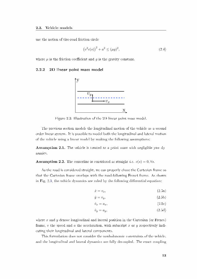
2.2.2 2D linear point mass model
x
y
Figure 2.3: Illustration of the 2D linear point mass model.
The previous section models the longitudinal motion of the vehicle as a second
order linear system. It is possible to model both the longitudinal and lateral motion
of the vehicle using a linear model by making the following assumptions:
Assumption 2.1. The vehicle is treated as a point mass with negligible yaw dy-
namics.
Assumption 2.2. The centerline is considered as straight i.e. c(s) = 0,∀s.
As the road is considered straight, we can properly chose the Cartesian frame so
that the Cartesian frame overlaps with the road-following Frenet frame. As shown
in Fig. 2.3, the vehicle dynamics are ruled by the following di�erential equation:
x = vx, (2.5a)
y = vy, (2.5b)
vx = ax, (2.5c)
vy = ay, (2.5d)
where x and y denote longitudinal and lateral position in the Cartesian (or Frenet)
frame, v the speed and a the acceleration, with subscript x or y respectively indi-
cating their longitudinal and lateral components.
This formulation does not consider the nonholonomic constraints of the vehicle,
and the longitudinal and lateral dynamics are fully decoupled. The exact coupling
13

Chapter 2. Preliminaries
between these dynamics involves nonlinear relations [19]; therefore, we approximate
it by an additional constraint. The vehicle heading θ can be reconstructed as θ =
arctan(vy/vx). We model the coupling of longitudinal and lateral dynamics by
enforcing condition θ ∈ [θ, θ], with
vy ∈ [vx tan(θ), vx tan(θ)]. (2.6)
To take into account the maximal tire force, we can limit the lateral acceleration
of the vehicle using the constraint similar to (2.3)
ay ∈ [ay, ay], (2.7)
An alternative approach is to use the tire-road friction circle as in (2.4).
Note that when the road is not straight, simply applying this model to the road-
following Frenet frame will induce modeling errors. The magnitude of the errors is
related to the road curvature.
2.2.3 Nonlinear point mass model
x
y
Figure 2.4: Illustration of the nonlinear point mass model.
The previous model is adequate for motion planning on highways or urban ar-
terial roads. However, the model mismatch becomes important if the longitudinal
dynamics is no longer dominant or if the road is not straight. In this case, it is
possible to consider a nonlinear point mass model incorporating the yaw dynamics
as shown in Fig. 2.4.
The model can be expressed in a Cartesian frame using the following equations:
14

2.2. Vehicle models
x = v cos θ, (2.8a)
y = v sin θ, (2.8b)
v = a, (2.8c)
θ = ω, (2.8d)
where v, θ are respectively the speed and the heading of the point mass. a and ω
are respectively the acceleration and the yaw rate.
Sometimes it is desirable to consider the vehicle motion in the road-following
Frenet frame. The above mentioned model can be transformed to the Frenet frame
as
s = v cos eθ
(1
1− rc(s)
), (2.9a)
r = v sin eθ, (2.9b)
v = a, (2.9c)
eθ = ω − v cos eθ
(c(s)
1− rc(s)
), (2.9d)
where s and r are coordinates in the Frenet frame, eθ is the alignment error, i.e., the
angle between the vehicle heading and the road centerline. The road information is
encoded in c(s), which is the curvature pro�le of the centerline.
Note that to avoid singularity in the di�erential equations, we must add a con-
straint
1− rc(s) > 0. (2.10)
Finally, the constraint derived from tire-road friction limit must be considered
as in (2.3) or (2.4).
2.2.4 Kinematic bicycle model
Bicycle models lump left and right wheels at the front (rear) axes together in the
modeling process. Comparing to point mass models, they are more realistic as they
consider the side-slip angle. Moreover, they have fewer states than a complete four-
wheel model, and they strike a good balance between complexity and realism. They
are widely used in the literature [19, 40] to plan trajectories or to control the vehicle.
Here we only consider one type of bicycle models: kinematic bicycle model.
As shown in Fig. 2.5, the kinematic bicycle model [39, 40] is governed by the
15

Chapter 2. Preliminaries
Figure 2.5: Kinematic bicycle model.
following nonlinear di�erential equations in the Cartesian frame
x = v cos(θ + β), (2.11a)
y = v sin(θ + β), (2.11b)
v = a, (2.11c)
θ =v
lrsin(β), (2.11d)
φ = ψ, (2.11e)
β = tan−1
(lr
lf + lrtan(φ)
), (2.11f)
where x and y are the coordinates of the center of mass. v, θ and φ are respectively
the speed, heading and the steering angle of the front wheel, β is the side-slip angle, a
and ψ are respectively the acceleration and the steering angular velocity. Eq. (2.11f)
is an algebraic equation connecting β and φ. lr and lf are respectively the distance
of the center of mass to the rear wheel and to the front wheel.
As in previous models, we must consider tire-road friction ( in (2.3) or (2.4))
limits when using kinematic bicycle model.
2.2.5 Concluding remarks
We have presented di�erent vehicle models that will be used in this thesis, ranging
from the double integrator for longitudinal motion to the kinematic bicycle model.
Point mass models are computationally cheap while they overly simplify the vehicle
dynamics. Therefore, it is adequate to use them in the planning stage. The kine-
16

2.3. Model predictive control
matic bicycle model strikes a good balance between complexity and realism. We
are going to show that it can be used for the tracking control in normal driving
conditions.
Note that this section does not aim at presenting a complete survey of vehicle
models: the dynamic bicycle model and four-wheel models are not presented. While
these models are essential if we want to control the vehicle in challenging scenarios
like emergency maneuvers, icy road or drift, they are not in the scope of this thesis.
A complete survey on vehicle models can be found in [39].
2.3 Model predictive control
k k+1 k+2 k+K
PAST FUTURE
...
Measured System Trajectory
Prediction Horizon
Predicted System Trajectory
Past Control Input
Predicted Control Input
Figure 2.6: Illustration of an MPC scheme.
Model Predictive Control (MPC), also known as Receding Horizon Control, has
been shown to be an attractive approach for the motion planning and control of
autonomous vehicles [19, 41, 18], thanks to its capability to systematically han-
dle vehicle dynamics, operating limits and on-road obstacles. MPC is a control
technique with the fundamental idea of using a model of the system to predict its
behavior up to a certain prediction horizon and generating control inputs that sat-
isfy the constraints and minimize a cost function (Fig. 2.6). The optimization is
repeated online at each sample time, in a receding horizon fashion, to take into ac-
count new measurements on the system state and the environment. Because of the
predictive nature of MPC, each optimization yields an optimal control trajectory for
the given prediction horizon as well as an optimal system trajectory. This speci�city
of MPC makes it suitable for both control and motion planning problems.
Traditionally, MPC has been applied to control dynamic systems with slow dy-
namics [42] as it was computationally expensive. However, recent advances in op-
timization algorithms [43, 44] have signi�cantly reduced the computation time of
MPC, thus clearing a major obstacle for automotive applications. In this section, we
introduce MPC formulations that will be applied to the motion planning and control
problems of individual autonomous vehicle or a group of autonomous vehicles in the
17

Chapter 2. Preliminaries
remaining chapters. Section 2.3.1 introduces the MPC formulation for systems in
which all states are real-valued. Section 2.3.2 presents the MPC formulation for
mixed logical dynamic systems in which some states can only have values of either
0 or 1.
2.3.1 Model predictive control for systems with real-valued states
We consider a generic dynamic system ξ(t) = f(ξ(t), u(t)), for example, an arbitrary
system presented in Section 2.2. Let ξ ∈ Rn and u ∈ Rm be the state vector and the
control input. We assume that all system states are continuously-valued. Without
loss of generality, we assume that the control inputs are piecewise constant with a
�xed sampling time τ , so that the dynamic can be discretized as
ξk+1 = fd(ξk, uk) (2.12)
where fd : Rn × Rm → Rn is the state update function with C1 continuity. The
system (2.12) is subject to the following state and input constraints,
ξk ∈ X , uk ∈ U ,∀k ≥ 0 (2.13)
where X and U are compact subsets of Rn and Rm. We shift the time horizon so
that the current time is k = 0. We assume that the full measurement of the state
ξ0 is available at the current time as ξ.
Let T be the prediction horizon of the MPC and let T = Kτ with K being the
number of time steps and τ being the discretization interval. We can then de�ne
the following �nite time optimal control problem to be solved at each time step,
minuJ (ξ,u), (2.14)
subj. to
ξ0 = ξ, (2.15a)
ξk+1 = fd(ξk, uk),∀k ∈ [0, ...,K − 1], (2.15b)
ξk ∈ X , uk ∈ U ,∀k ∈ [0, ...,K], (2.15c)
ξK ∈ Xf , (2.15d)
where ξk is the predicted state at time k. ξ = [ξ0, ..., ξK ] is the state trajectory
obtained by applying the control sequence u = [u0, ..., uK−1] to the system starting
from the initial state ξ. Equation (2.15d) is the terminal constraint with Xf being
18

2.3. Model predictive control
a compact set in Rn.The cost function J (ξ,u) is a C1 function de�ned in its generic form as
J (ξ,u) =
K−1∑k=0
L(ξk, uk) + G(ξK) (2.16)
where L(·, ·) is the running cost and G(·, ·) is the terminal cost.
The solution of the problem (2.14) is the optimal control input de�ned as u∗ =
[u0,∗, ..., uK−1,∗]. Applying u∗ to the system (2.12) results in the (predicted) optimal
state trajectory ξ∗ = [ξ0,∗, ..., ξK,∗].
In traditional MPC schemes, the �rst sample of u∗ (in interval [0, τ) ) is applied
to control the system and the optimization problem is reformulated and solved at
the next sampling time. However, when (2.12) is just a simpli�ed approximation of
the real system dynamics and a low-level tracking controller exists, we may discard
u∗ and pass the state trajectory ξ∗ to the tracking controller. In this case, the MPC
controller actually becomes a motion planner that plans the system trajectory.
The optimization problem is a continuous optimization problem with 2(m +
n)K variables, nK equality constraints (from (2.15b)) and a number of inequality
constraints (from (2.15c) and (2.15d)). The computational complexity of the MPC
is polynomial to the number of variables and constraints. Depending on the (non-
)linearity and (non-)convexity of the cost function and the constraints, di�erent
numeric methods may apply to solve the problem. If the cost function (2.16) is in
quadratic form and all constraints are linear, the optimization problem is reduced
to a Quadratic Program (QP) for which e�cient algorithms exists. On the other
hand, if the cost function is not quadratic and/or some constraints are nonlinear, we
must rely on Interior Point or Sequential Quadratic Programming algorithms [45]
which are in general less e�cient than QP solvers. Remark that since these solvers
rely on gradient descent to minimize the cost function, they can be trapped in local
optima if the cost function or some constraints are non-convex.
2.3.2 Model predictive control of hybrid systems
Dynamic systems are traditionally described using a set of di�erential or di�erence
equations, typically derived from physical laws. However, in many applications,
the considered system also contains discrete-valued signals along with real-valued
signals. We refer to systems with both continuous variables and discrete variables
as hybrid systems.
General hybrid systems with nonlinear di�erential or di�erence equations are
hard to control. Here we consider a special type of hybrid systems called the Mixed
19

Chapter 2. Preliminaries
Logical Dynamic Systems, which can be described by the following relations in
discrete time:
ξk+1 = Aξk +B1uk +B2σ
k +B3zk +B4, (2.17a)
C1ξk + C2u
k + C3σk + C4z
k + C5 ≤ 0, (2.17b)
where ξ ∈ Rnc × {0, 1}nl is a vector of continuous and binary states, u ∈ Rmc ×{0, 1}ml are inputs, σ ∈ {0, 1}rl are auxiliary binary variables and z ∈ Rrc are
continuous auxiliary variables. Capital letters represent matrices of suitable dimen-
sions. Eq. (2.17a) de�nes the state transition rule of the system. Eq. (2.17b) is the
collection of state and control constraints.
Similar to real-valued systems, MPC can be applied to control hybrid systems.
The MPC problem can then be referred as hybrid MPC (hMPC). Wet let the current
time be k = 0 and let the full measurement of the state ξ0 as ξ. Let T be the
prediction horizon of the MPC and T = Kτ with K be the number of time steps
and τ the discretization resolution. We can de�ne the following �nite time optimal
control problem to be solved at each time step:
minuJ (ξ,u,σ, z), (2.18)
subj. to
ξ0 = ξ, (2.19a)
ξk+1 = Aξk +B1uk +B2σ
k +B3zk +B4, k ∈ [0, ...,K − 1], (2.19b)
C1ξk + C2u
k + C3σk + C4z
k + C5 ≤ 0, k ∈ [0, ...,K − 1], (2.19c)
ξK ∈ Xf , (2.19d)
where ξ,u,σ, z are respectively vectors for state, control, auxiliary discrete variable
and auxiliary continuous variables. Similar to real-valued MPC, the solution of the
problem (2.18) is the optimal control input u∗ with the optimal state trajectory ξ∗
as by product; the cost function can also be decomposed to running cost terms and
a terminal cost as in the real-valued case.
The optimization problem is a Mixed-Integer Programming (MIP) problem.
General MIP problems are hard to solve, but e�cient algorithms exist for special
instances of MIP, notably Mixed-Integer Linear Programming (MILP) and Mixed-
Integer Quadratic Programming (MIQP). Problem (2.18) becomes MILP if the cost
function and all constraints are linear. MILP problems can be solved by linear pro-
gramming based branch-and-bound algorithms. On the other hand, problem (2.18)
20

2.3. Model predictive control
is a MIQP if the cost function is quadratic while constraints are linear. Branch-
and-bound methods based on quadratic programming can be employed to e�ectively
solve the problem. Widely available solvers of MILP and MIQP include CPLEX [46]
and Gurobi [44].
2.3.3 Feasibility, stability and robustness
Feasibility of the optimization problem at each sample time must be ensured for
the formulated MPC problem. Infeasibility usually rises from the constraints that
have some extrinsic variables. For example, in automotive applications, obstacle
avoidance constraints contain variables representing the current and future states
of obstacles. The values of these variables at k = 0 are usually measured with
noisy sensors and the future values are predicted using prede�ned motion models.
An optimization problem that is feasible at the current sample time may become
infeasible at the next instant when incorporating new measurements. A possible
way to preserve feasibility is to consider all possible values of these variables in the
constraint formulation, for example, using the notion of maximal invariant set [47],
so that we have a theoretical feasibility guarantee for the next sample time if the
current one is feasible. A simpler alternative is to convert the concerned constraints
to soft constraints. For example, a constraint C1x + C2u + C3 ≤ 0 is softened to
C1x+ C2u+ C3 ≤ ε with ε ≥ 0. An additional term Mε2 is also added to the cost
function with M being a large constant. In this way, small violations of constraints
are tolerated while strongly penalized to preserve feasibility. Both methods are used
in this thesis.
Informally speaking, an MPC formulation is said to be stable if the system
is controlled to asymptotically converge to a desired equilibrium. The theoretical
guarantee of stability is usually achieved by combining a properly designed terminal
cost G(ξK) with a terminal constraint ξK ∈ Xf [48]. However, such design usually
increases the computational complexity of the optimization problem. Moreover, in
automotive applications, the desired equilibrium points change frequently. Thus, a
common practice [19, 21] is to ignore the terminal cost and terminal constraints and
to verify the stability by extensive simulations and experiments. Naturally, in this
way we lose the theoretical guarantee of stability. This thesis adopts the common
practice to only consider experimental stability.
Uncertainties exist in the modeling of vehicle dynamics and in the measurement
of vehicle states, which raise the problem of robustness for MPC. In more details, we
refer to robust stability and robust constraint satisfaction if the respective property
is guaranteed under bounded uncertainties. It has been shown that naive MPC
21

Chapter 2. Preliminaries
formulation without any robustness consideration is intrinsically robust to small
uncertainties thanks to its predictive nature [49]. On the other hand, various robust
MPC formulations are discussed in the literature such as Min-Max [50], constraint-
tightening MPC [51], tube based MPC [52] and multi-stage MPC [53]. Notably,
tube based MPC has been applied to robustly control autonomous vehicles to avoid
obstacles [54]. This thesis does not consider the problem of robustness, while all
MPC formulations in the remaining chapters can be augmented to their robust
counterpart by following the tube-based methodology.
22
Chapter 3
Model Predictive Control for
Autonomous Driving
This chapter presents the design of a nonlinear MPC based control framework for
autonomous driving. We consider a hierarchical design that decomposes the con-
troller into a motion planner and a tracking controller. At the motion planning
level, MPC is used to compute collision-free reference trajectories using the nonlin-
ear point mass model. At the tracking control level, an MPC controller based on the
kinematic bicycle model computes control inputs that track the high-level reference
trajectories. Simulations are performed to validate the approach. Note that ideas
similar to those presented in this chapter can be found in [19, 55]. Nevertheless,
this chapter di�ers signi�cantly from [19, 55] as we use di�erent vehicle models and
consider obstacle avoidance constraints di�erently. The proposed design will serve
as a basis for the rest of the thesis.
3.1 Introduction
An important research area for autonomous vehicles is the design of a robust and
e�cient control framework that guides autonomous vehicles to proceed in an en-
vironment governed by tra�c rules and populated with obstacles and other tra�c
participants. Single-level controller designs that map road situations directly to
vehicle controls exist in the literature [9, 10]. However, for computational reasons,
most literature designs the control framework in a hierarchical way, with a high-level
motion planning (or trajectory planning) module that computes feasible trajectories
using simpli�ed vehicle model and considering the environment information, and a
low-level tracking controller that tracks the trajectories. With such design, the com-
putationally intensive motion planner can run at a relatively low frequency and the
tracking controller can run at a high frequency.
Under this hierarchical philosophy, many motion planning frameworks [13, 14,
15, 56, 16, 17] have been proposed in the literature, which can be roughly divided into
three categories of approaches: path-velocity decomposition approaches, sampling
based approaches and Model Predictive Control (MPC) based approaches.
Chapter 3. Model Predictive Control for Autonomous Driving
The path-velocity decomposition technique [57] breaks down the motion plan-
ning problem into two sub-problems: path planning and velocity planning. The
path planning problem determines a kinematically feasible (curvature-continuous)
path along the road. Various path generation methods are proposed using cubic
curvature polynomials [58], Bézier curves [56, 59], clothoid tentacles [60], Dubin's
paths [61], and nonlinear optimization techniques [17]. The velocity planning prob-
lem generates a speed pro�le that is adapted to the previously generated path.
Some work [62, 17, 63] assumes the velocity pro�le to have certain shape (poly-
nomial, trapezoidal, etc.) and samples some terminal states to generate a set of
pro�les. A best pro�le for the chosen cost function is then selected.
Sampling based approaches [13, 14, 15] sample directly the state space of the
autonomous vehicle to obtain a set of feasible trajectories, and then select the best
one to execute according to a cost function. Deterministic sampling approaches [13]
discretize the state space using a spatiotemporal lattice. Graph search methods
are then adopted to �nd the optimal trajectory. The disadvantage of deterministic
sampling is that it is only resolution complete, meaning that the produced trajectory
is only resolution-optimal. In order to mitigate this problem, stochastic sampling
approaches [14, 15] are proposed using Rapidly Exploring Random Tree Star (RRT*)
and its variants. RRT* is powerful in exploring the state space and is asymptotically
complete (the optimal trajectory can be found eventually with a probability of 1).
However, the convergence speed towards the optimal trajectory is usually slow.
The downside of sampling based approaches is that they spend a large amount
of computation resources to generate and evaluate a large set of trajectories, while
most of them are discarded. Model Predictive Control (MPC) based methods [18, 64]
formulate the trajectory generation problem as an optimization problem over the
state space and use gradient-descending techniques to �nd the optimal trajectory.
The optimization problem is solved in a periodic fashion with a limited horizon to
take into account new environmental information. This category of approaches is
e�cient in �nding the optimal trajectory with the help of the gradient information.
Furthermore, MPC-based approach permits high-precision planning, for example,
keeping a precisely given distance from its preceding vehicle, thanks to its optimiza-
tion nature.
Rich literature also exists for controlling the vehicle to track a reference trajec-
tory. Notably, reference [65] presents a sliding mode controller design; reference [66]
utilizes the notion of �atness to control the lateral dynamics; and reference [67]
presents a model free approach to design the controller. As discussed in � 2.3, MPC
is applicable both in motion planning and vehicle control, thus some work [19, 10]
designs MPC-based tracking controllers using vehicle models of various degrees of
24

3.2. Control architecture overview
complexity.
In this chapter, we will present the applications of MPC to the motion planning
and the control of autonomous vehicles. More speci�cally, in � 3.2, we present
the overview a hierarchical control architecture based on MPC. � 3.3 considers the
modeling of obstacles. In � 3.4 we detail the motion planner design and in � 3.5
presents the tracking controller. � 3.6 presents simulations and � 3.7 concludes this
chapter.
3.2 Control architecture overview
MPC based Motion Planner
MPC based Tracking Controller
Acc/Braking Logic
Vehicle
ObstacleInformation
Scenario Specification
Figure 3.1: Two-level control architecture based on MPC.
The philosophy of hierarchical MPC design is to separate the planning stage and
the control stage and optimize each one in parallel to improve global e�ciency. At
the planning level, an MPC controller uses a simpli�ed vehicle model to compute
dynamically feasible trajectories that avoid obstacles. At the control level, another
MPC controller is used to track the reference trajectory generated by the planner
using a more complete vehicle model without considering obstacles. Using such
design, the planner can run at a relatively low frequency, thus it can use a longer
prediction horizon and consider more on-road objects. On the other hand, the
controller can run at a high frequency since it can use a short prediction horizon
and does not need to consider obstacles.
25

Chapter 3. Model Predictive Control for Autonomous Driving
Fig. 3.1 illustrates the hierarchical control design. The current vehicle state ξ
is measured from the vehicle using sensors and is fed to both the planner and the
controller. The motion planner also takes as input the reference trajectory ξref ,
representing the desired trajectory if no obstacle is present. A simple form of ξrefcan be a constant speed pro�le. The obstacle information contains the positions,
shapes, trajectory predictions and other information of on-road obstacles obtained
from the fusion of di�erent sensors with the digital maps. The scenario speci�ca-
tion interface allows upper level components to re-con�gure and/or re-parameterize
the planner based on the current driving scenario (e.g., highway cruising, highway
merging/exiting, urban intersections, heavy rain/fog with exceptional speed lim-
its). This interface is necessary since di�erent scenarios can lead to di�erent sets
of constraints and di�erent planner parameters. The motion planner generates the
optimal trajectories ξ∗, which is then converted to the reference trajectory ξc,reffor the tracking controller. Subscripts p and c are respectively used to label the
planner and the controller. The tracking controller computes the optimal control
inputs (acceleration and steering) that best follow ξc,ref . The acceleration inputs
are fed to the acceleration/braking logic module to control the torques exerted on
the wheels. The steering inputs are directly applied to the vehicle.
Detailed planner and tracking controller designs are described in � 3.4 and � 3.5.
3.3 Obstacle Models
AB
Figure 3.2: Obstacle classi�cation.
A major task for autonomous driving is to avoid on-road obstacles including
other tra�c participants, objects on the road and road works. Since obstacles
may have di�erent sizes, shapes and dynamics, di�erent avoidance strategies are
required. For example, an autonomous vehicle can avoid bicyclists by swerving
around them without changing its lane, while for a slow vehicle driving in the front,
the autonomous vehicle must decelerate to avoid rear-end collision (unless a lane
change command is issued).
In this section, we study two di�erent models for on-road objects. We �rst
classify objects into two categories:
26

3.3. Obstacle Models
• Lane-Blocking Obstacles (LBOs). Static or dynamic obstacles that block
one or more lanes (e.g. Obstacle A in Fig. 3.2).
• Non-Blocking Obstacles (NBOs). Static or dynamic obstacles that only
block a small part of a lane such that autonomous vehicles can swerve to avoid
them and proceed (e.g. Obstacle B in Fig. 3.2) .
Note that the classi�cation for an object may change overtime considering the
current driving context. For example, a bicyclist at the border of the current lane can
be considered as an NBO unless we detect that he/she decides to cross the road. In
this situation, he/she should be considered as an LBO since the autonomous vehicle
must wait until the bicyclist has passed to proceed. As the focus of this thesis is
on vehicle control, we assume that obstacle classi�cations are provided in a timely
manner through the obstacle information interface by the perception algorithm.
We consider the obstacle modeling in the road-following Frenet frame. Di�erent
models apply for LBOs and NBOs. Let o denote an obstacle and po = [so, ro] be the
(potentially time-varying) Frenet coordinate of the obstacle. A vehicle must keep
a safe distance from LBOs to avoid rear-end crashes unless it changes its lane. A
simple linear constraint can be de�ned as
s+ vTgap ≤ so, (3.1)
where Tgap is the desired time gap.
MarginObstacle Parabola
Figure 3.3: Approximation of obstacle region by a parabola.
A vehicle is able to swerve to avoid NBOs. However, in many cases, NBOs cre-
ate multiple maneuver variants, e.g., a vehicle may swerve in clock-wise or counter
clock-wise manner. This problem is widely known as the combinatorial nature of
autonomous driving [2]. Moreover, the shapes of obstacles are usually irregular
and non-smooth. Therefore, approximations are required to incorporate obstacle
avoidance conditions into the nonlinear MPC scheme. Fig. 3.3 illustrates the ap-
27

Chapter 3. Model Predictive Control for Autonomous Driving
proximation method used in this chapter. For an arbitrary NBO, we �rst adopt
the heuristic to assign it to the nearest border of the road. Proper margins are
then added to the NBO to take into account the size of the vehicle and convert the
(potentially irregular) obstacle region into an enhanced obstacle region of rectangle
shape. Finally the enhanced obstacle region is approximated using a continuous and
di�erentiable parabolic constraint that crosses two vertices of the enhanced obstacle
region. For an obstacle a�ected to the lower lane boundary, the constraint is given
as
− r + (as2 + bs+ c) ≤ 0, (3.2)
and for an obstacle a�ected to the upper lane boundary, the constraint is given as
r − (as2 + bs+ c) ≤ 0. (3.3)
The unknown coe�cients a, b, c can be calculated by solving the following linear
system. s2o,0 so,0 1
s2o,1 so,1 1
s2o,2 so,2 1
abc
=
ro,0ro,1
ro,2
, (3.4)
where [so,0, ro,0] is the vertex of the parabola and [so,i, ro,i], j ∈ {2, 3} are the onlytwo points where the enhanced obstacle region intersects with the parabola.
Note that this approximation method inevitably overestimates the occupancy of
an NBO on the road space. If the on-road environment is cluttered, more precise
estimation will be necessary using higher degree polynomials or other nonlinear
functions.
We compactly written the mentioned obstacle avoidance conditions for LBOs
and NBOs as: ∀o,h(ξ, po) ≤ 0. (3.5)
28

3.4. Motion planner
3.4 Motion planner
We consider the MPC formulation for the motion planner. We recall the nonlinear
point mass model in the Frenet frame (2.9) discussed in Section 2.2.3:
s = v cos eθ
(1
1− rc(s)
), (3.6a)
r = v sin eθ, (3.6b)
v = a, (3.6c)
eθ = ω − v cos eθ
(c(s)
1− rc(s)
). (3.6d)
We de�ne ξ = [s, r, v, eθ] as the state vector. s and r are respectively the longi-
tudinal and lateral coordinates of the vehicle. v is the vehicle speed and eθ is the
heading error. The control inputs are u = [a, ω], with the �rst component being the
acceleration and the second one being the yaw rate. We compactly write the model
as ξ = f(ξ, u).
To take into account the dynamic limitations of the vehicle, we de�ne bounds as
ξ ∈ [ξ, ξ], u ∈ [u, u], (3.7)
and we require
ξ = [−∞, r, 0, eθ], ξ = [+∞, r, v, eθ],u = [a, ω], u = [a, ω].
(3.8)
Let T be the prediction horizon of the planner and K be the number of steps.
Let ξ = [ξ0, ..., ξK ] and u = [u0, ..., uK ] be the vector of states and control inputs.
Consider the following cost function in least-square form:
J (ξ,u) =K∑k=0
(||ξk − ξkp,ref ||2Q + ||uk||2R, (3.9)
where ξp,ref is the state reference. Q and R are two positive diagonal matrices with
proper dimension. The MPC for planning is formulated as
minuJ (ξ,u) +M
∑∀o
(εko
)2,
29
Chapter 3. Model Predictive Control for Autonomous Driving
Previously Planned Trajectory
Currently Planned Trajectory
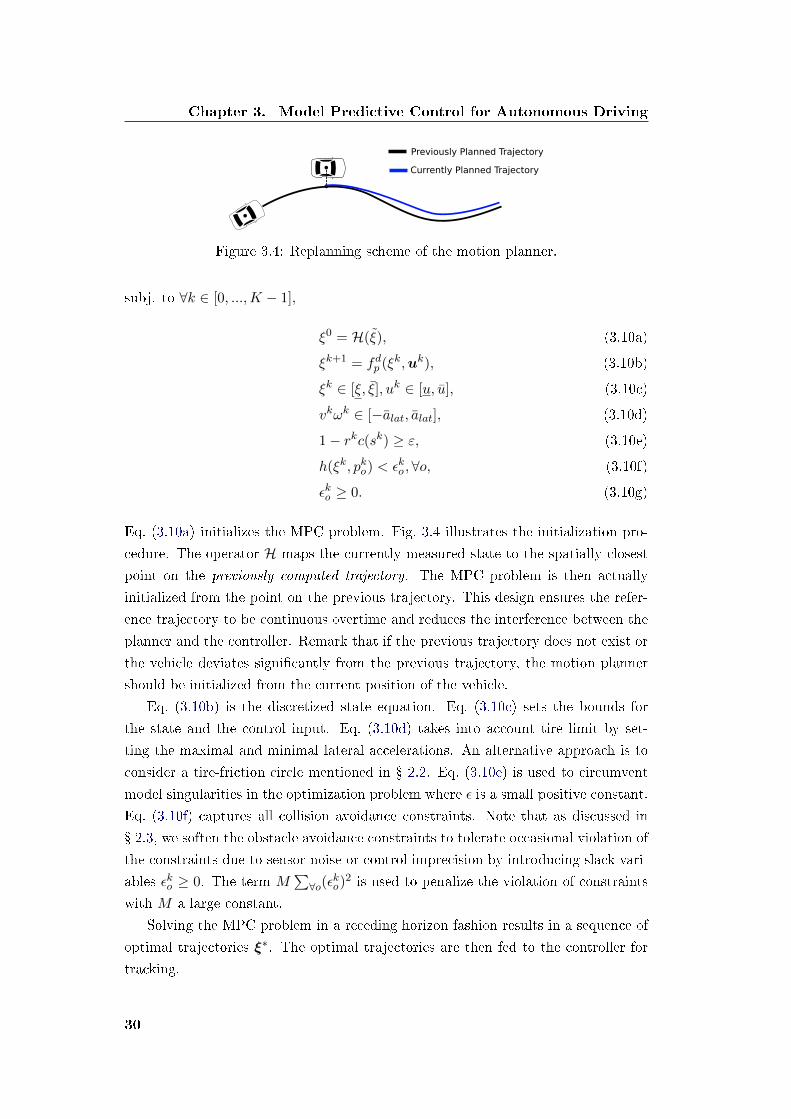
Figure 3.4: Replanning scheme of the motion planner.
subj. to ∀k ∈ [0, ...,K − 1],
ξ0 = H(ξ), (3.10a)
ξk+1 = fdp (ξk,uk), (3.10b)
ξk ∈ [ξ, ξ], uk ∈ [u, u], (3.10c)
vkωk ∈ [−alat, alat], (3.10d)
1− rkc(sk) ≥ ε, (3.10e)
h(ξk, pko) < εko ,∀o, (3.10f)
εko ≥ 0. (3.10g)
Eq. (3.10a) initializes the MPC problem. Fig. 3.4 illustrates the initialization pro-
cedure. The operator H maps the currently measured state to the spatially closest
point on the previously computed trajectory. The MPC problem is then actually
initialized from the point on the previous trajectory. This design ensures the refer-
ence trajectory to be continuous overtime and reduces the interference between the
planner and the controller. Remark that if the previous trajectory does not exist or
the vehicle deviates signi�cantly from the previous trajectory, the motion planner
should be initialized from the current position of the vehicle.
Eq. (3.10b) is the discretized state equation. Eq. (3.10c) sets the bounds for
the state and the control input. Eq. (3.10d) takes into account tire limit by set-
ting the maximal and minimal lateral accelerations. An alternative approach is to
consider a tire-friction circle mentioned in � 2.2. Eq. (3.10e) is used to circumvent
model singularities in the optimization problem where ε is a small positive constant.
Eq. (3.10f) captures all collision avoidance constraints. Note that as discussed in
� 2.3, we soften the obstacle avoidance constraints to tolerate occasional violation of
the constraints due to sensor noise or control imprecision by introducing slack vari-
ables εko ≥ 0. The term M∑∀o(ε
ko)
2 is used to penalize the violation of constraints
with M a large constant.
Solving the MPC problem in a receding horizon fashion results in a sequence of
optimal trajectories ξ∗. The optimal trajectories are then fed to the controller for
tracking.
30
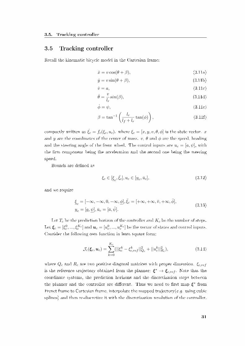
3.5. Tracking controller
3.5 Tracking controller
Recall the kinematic bicycle model in the Cartesian frame:
x = v cos(θ + β), (3.11a)
y = v sin(θ + β), (3.11b)
v = a, (3.11c)
θ =v
lrsin(β), (3.11d)
φ = ψ, (3.11e)
β = tan−1
(lr
lf + lrtan(φ)
), (3.11f)
compactly written as ξc = fc(ξc, uc). where ξc = [x, y, v, θ, φ] is the state vector. x
and y are the coordinates of the center of mass. v, θ and φ are the speed, heading
and the steering angle of the front wheel. The control inputs are uc = [a, ψ], with
the �rst component being the acceleration and the second one being the steering
speed.
Bounds are de�ned as
ξc ∈ [ξc, ξc], uc ∈ [uc, uc], (3.12)
and we require
ξc
= [−∞,−∞, 0,−∞, φ], ξc = [+∞,+∞, v,+∞, φ],
uc = [a, ψ], uc = [a, ψ].(3.13)
Let Tc be the prediction horizon of the controller and Kc be the number of steps.
Let ξc = [ξ0c , ..., ξ
Kcc ] and uc = [u0
c , ..., uKcc ] be the vector of states and control inputs.
Consider the following cost function in least-square form:
Jc(ξc,uc) =
Kc∑k=0
(||ξkc − ξkc,ref ||2Qc+ ||ukc ||2Rc
), (3.14)
where Qc and Rc are two positive diagonal matrices with proper dimension. ξc,refis the reference trajectory obtained from the planner: ξ∗ → ξc,ref . Note that the
coordinate systems, the prediction horizons and the discretization steps between
the planner and the controller are di�erent. Thus we need to �rst map ξ∗ from
Frenet frame to Cartesian frame, interpolate the mapped trajectory(e.g. using cubic
splines) and then re-discretize it with the discretization resolution of the controller.
31

Chapter 3. Model Predictive Control for Autonomous Driving
ξ = [−∞,−3 m, 0 m/s,−0.4 rad], ξ = [+∞, 3 m, 25 m/s, 0.4 rad],u = [−4.5 m/s2,−0.4 rad/s], u = [2.5 m/s2, 0.4 rad/s],
alat = 1.5 m/s2,M = 100000, T = 5.0 s,K = 25, Q = [0, 10, 2, 100], R = [5, 200],ξc
= [−∞,−∞, 0,−∞,−0.5 rad], ξc = [+∞,+∞, 25 m/s,+∞, 0.5 rad],uc = [−6 m/s2,−0.5 rad/s], uc = [4 m/s2, 0.5 rad/s],T = 1.6 s,K = 8, Qc = [3, 2, 5, 2], Rc = [0.8, 10],
Table 3.1: Parameters used for the proposed control design
The MPC controller is then formulated as
minuc
Jc(ξc,uc),
subj. to ∀k ∈ [0, ...,Kc − 1],
ξk+1c = fdc (ξkc ,u
kc ), (3.15a)
ξkc ∈ [ξc, ξc], u
kc ∈ [uc, uc]. (3.15b)
The solution of the MPC problem is the optimal acceleration pro�le and the
optimal steering speed pro�le. Since the vehicle is controlled by steering, we feed
the acceleration and the steering angle (instead of the steering speed) to the vehicle.
3.6 Simulations
In this section, we use extensive simulations to illustrate the performance of the
proposed control architecture. We have implemented our framework in the robotic
simulator Webots [68]. The control algorithms are coded in C++ and we use the
ACADO toolkit [43] to solve the MPC problems. Simulations were performed on a
personal computer running on a 3.4 GHz Intel Core i7 CPU with 32GB of RAM.
Table 3.1 captures the parameters that are common in all test cases. Vehicle
length is set to 4 m and width 3 m. The motion planner replans every 256 ms and
the tracking controller recalculates the control input every 32 ms. Scenario-speci�c
parameters will be introduced respectively in each case study.
3.6.1 Static NBO avoidance
Scenario description
We consider the problem of avoiding static NBOs during high speed autonomous
driving on a straight road segment. The goal is to illustrate the capacity of the
proposed architecture to handle static obstacles. The motion planner is con�gured
to stay in the road centerline if possible and to track a constant speed pro�le of
32

3.6. Simulations
0 50 100 150 200 2503-
EV0
3
x(m)
y(m)
Figure 3.5: Illustration of the simulation setup for the static obstacle avoidancescenario. EV stands for Ego Vehicle.
20 m/s. Four obstacles are distributed along the road segment as illustrated in
Fig. 3.5. Obstacles are assumed to be 4 m wide and 6 m long. The chosen bounding
parabolas for obstacle regions are illustrated using dotted red lines. We assume that
the sensors of the ego vehicle have a detection range of 80 m, thus only obstacles
within the range will be considered by the controller.
Simulation results
We �rst perform the simulation assuming perfect localization. Fig. 3.6a illustrates
the vehicle trajectory and Fig. 3.6b presents the speed and steering pro�les of the
vehicle. We observe that the vehicle decelerates when approaching the obstacles
(to satisfy the constraint on the lateral acceleration) and successfully avoids four
obstacles.
To demonstrate the robustness of the control architecture with respect to lo-
calization errors, we disturb the GPS signal with a uniformly chosen random error
inside [−0.5 m, 0.5 m]. No �ltering technique is used to smooth the GPS signal. The
simulation result is presented in Fig. 3.7. We notice that the ego vehicle is still
able to plan and track collision-free trajectories. The fact that we replan from the
nearest point on the previous trajectory rather than the current position enhances
the stability of the planned trajectories.
3.6.2 Dynamic NBO avoidance
Scenario description
We consider the scenario illustrated in Fig. 3.8 in which a vehicle needs to circumvent
a cyclist at the border of the road. The goal is to illustrate the capacity of the
proposed architecture in handling dynamic obstacles. The vehicle is tracking the
road centerline with a constant speed pro�le of 15 m/s. The cyclist moves at a speed
33

Chapter 3. Model Predictive Control for Autonomous Driving
0 50 100 150 200−3
0
3
x(m)
y(m)
Predict ion EV
(a)
0 5 10 150
5
10
15
20
25
t(s)
v(m/s)
0 5 10 15−0.25
0
0.25
φ(rad)
v φ
(b)
Figure 3.6: Perfect localization. (a) The trajectory of the ego vehicle as well asthe predicted trajectories of the motion planner. (b) The vehicle speed and vehiclesteering angle during the simulation.
of 4 m/s. The obstacle region of the cyclist is chosen conservatively to be 2 m wide
and 3 m long.
We assume that the trajectory predictions of the cyclist are provided by the
perception component. In the simulation, the cyclist is assumed to maintain con-
stant speed during the prediction horizon. The vehicle localization is assumed to be
perfect.
Simulation results
Fig. 3.9a illustrate the trajectory of the ego vehicle. We observe that the ego vehicle
successfully circumvents the cyclist.
3.6.3 Lane change at the presence of an LBO
Scenario description
We consider the scenario illustrated in Fig. 3.10 in which the ego vehicle is approach-
ing a slow vehicle (considered as an LBO) driving at a constant speed of 10 m/s. The
initial speed and the desired speed of the ego vehicle are both set to 15 m/s. Since
34

3.6. Simulations
0 50 100 150 200−3
0
3
x(m)
y(m)
Predict ion EV
(a)
0 5 10 150
5
10
15
20
25
t(s)
v(m/s)
0 5 10 15−0.25
0
0.25
φ(rad)
v φ
(b)
Figure 3.7: Imperfect localization with 0.5m error. (a) The localization signal ofthe ego vehicle as well as the predicted trajectories of the motion planner. (b) Thevehicle speed and vehicle steering angle during the simulation.
0 20 40 60 80−3
0
3
x(m)
y(m) EV Cyclist
Figure 3.8: Illustration of the scenario of dynamic obstacle avoidance.
the slow vehicle is blocking lane 0, the ego vehicle must adapt its speed to avoid
rear-end collision. At simulation time t = 10 s, the controller receives a lane change
command to lane 1 (achieved by modifying the desired o�set rref from 0 to 6 m).
The constant time gap from the slow vehicle Tgap is set to 2 s. In the simulation, the
slow vehicle is assumed to maintain constant speed during the prediction horizon.
The vehicle localization is assumed to be perfect.
Simulation results
Fig. 3.11a illustrates the trajectory of the ego vehicle. We notice that the vehicle �rst
decelerate to synchronize its speed with the slow vehicle in the front. At t = 10 s,
35

Chapter 3. Model Predictive Control for Autonomous Driving
0 20 40 60 80−3
0
3EV position
Cyclist position
x(m)
y(m)
Predict ion EV
0 12
34
5
0 1 2 3 4 5
(a)
0 2 40
5
10
15
20
t(s)
v(m/s)
0 2 4−0.1
0
0.1
φ(rad)
v φ
(b)
Figure 3.9: Dynamic obstacle avoidance. (a) The trajectory of the ego vehicle aswell as the predicted trajectories. We mark the positions of the vehicle and thecyclist at six di�erent time instants using natural numbers and color codes (lightercolor means further time instant). (b) Speed pro�le and steering pro�le of the egovehicle.
0 50 100 150 200 250 300−3
0
3
6
9
x(m)
y(m)
EV Slow Vehicle
Lane 0
Lane 1
Figure 3.10: Illustration of the scenario of lane change.
the controller receives the lane change command and plans a dynamically feasible
trajectory towards lane 1. The ego vehicle then recovers its desired speed in lane 1.
36
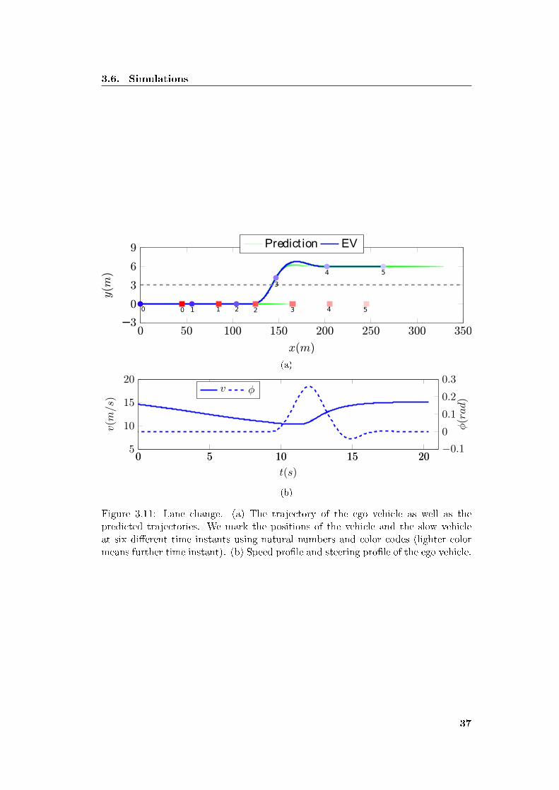
3.6. Simulations
0 50 100 150 200 250 300 350−3
0
3
6
9
x(m)
y(m)
Predict ion EV
0 1 2 3 4 50 1 2
3
4 5
(a)
0 5 10 15 205
10
15
20
t(s)
v(m/s)
0 5 10 15 20−0.1
0
0.1
0.2
0.3
φ(rad)
v φ
(b)
Figure 3.11: Lane change. (a) The trajectory of the ego vehicle as well as thepredicted trajectories. We mark the positions of the vehicle and the slow vehicleat six di�erent time instants using natural numbers and color codes (lighter colormeans further time instant). (b) Speed pro�le and steering pro�le of the ego vehicle.
37
Chapter 3. Model Predictive Control for Autonomous Driving
Computation time
Fig. 3.12 gives the evolutions of computation time for the three presented scenarios.
We observe that the computation time for the motion planner stays in the range
of [40 ms, 150 ms]. Notably, complex scenarios (static/dynamic obstacle avoidance)
cost the planner more time to �nd the optimal solutions. Nevertheless, computation
time in all scenarios is less than the replanning period (256 ms). The computation
time of the tracking controller remains below the replanning period of the controller
(32 ms), demonstrating the e�ciency of the MPC based tracking controller.
0 5 10 150
50
100
150
200
250
t(s)
Comp.Tim
e(m
s)
Planner Controller
(a)
0 3 6 90
50
100
t(s)
Comp.Tim
e(m
s)
Planner Controller
(b)
0 5 10 15 200
50
100
150
t(s)
Comp.Tim
e(m
s)
Planner Controller
(c)
Figure 3.12: Computation time for the motion planner and the tracking controller.(a) static obstacle avoidance (perfect localization). (b) dynamic obstacle avoidance.(c) lane change.
38

3.7. Concluding remarks
3.7 Concluding remarks
We have presented a hierarchical design of the control architecture for autonomous
driving with a nonlinear MPC based motion planner for trajectory generation and
a nonlinear MPC based controller to follow the generated trajectories. Simulations
have demonstrated the e�ectiveness of the proposed approach.
One major requirement for nonlinear MPC is that its constraints must be dif-
ferentiable. However, on-road autonomous driving often leads to non-di�erentiable
or even non-continuous constraints. For example, the surface of a polytope-shaped
obstacle is non-di�erentiable. In this chapter, we used bounding parabolas to ap-
proximate obstacle regions to create di�erentiable constraints, which leads to over-
estimation of the area of the obstacle region. Is there a way to incorporate non-
di�erentiable constraints into the proposed framework? In the next chapter, a novel
hybrid MPC based motion planner will be proposed to consider both di�erentiable
and non-di�erentiable constraints.
39


Chapter 4
Model Predictive Control for
Autonomous Driving Integrating Logical
Constraints
In this chapter we design a hybrid Model Predictive Control (hMPC) motion plan-
ner for autonomous driving. In the previous chapter, we formulated the motion
planning problem as a nonlinear program with di�erentiable cost functions and con-
straints. Gradient-based optimization methods were then used to �nd the optimal
trajectory. However, these methods are ill-suited for logical constraints such as those
raised by tra�c rules, presence of obstacles and, more importantly, to the existence
of multiple maneuver variants. We propose a new hMPC design of the motion plan-
ner to formulate the trajectory generation problem as a Mixed-Integer Quadratic
Program. This formulation can be solved e�ciently using widely available solvers,
and the resulting trajectory is guaranteed to be globally optimal. We apply our
framework to several scenarios that are still widely considered as challenging for
autonomous driving, such as obstacle avoidance with multiple maneuver choices,
intersection crossing, overtaking with oncoming tra�c or optimal lane-change deci-
sion making. Simulation results and �eld experiments demonstrate the e�ectiveness
of our approach and its real-time applicability.
4.1 Introduction
In Chapter 3, we have presented a MPC based motion planner which translates the
planning problem into a nonlinear optimization problem. The simulation results
have shown that the proposed planner works well with di�erentiable cost functions
and constraints. However, the context of on-road autonomous driving also leads to
a di�erent family of constraints, referred to as logical constraints because they can
be naturally formulated as propositional logic rules.
The �rst source of logical constraints is tra�c rules and expected driving behav-
iors, for instance:
• If a vehicle is on a speed bump, then it must drive slowly.

Chapter 4. Model Predictive Control for Autonomous Driving
Integrating Logical Constraints
• If a vehicle wants to exit the highway, it must be on the exit lane.
These rules with �if-else� structures can be easily mapped to logical proposi-
tions. Moreover, driving generally involves discrete decisions among multiple ma-
Figure 4.1: Illustration of multiple maneuver variants for the white car in an over-taking scenario. Adapted from Fig. 1 of [2].
neuver variants, which makes trajectory planning combinatorial in nature [2, 69, 70].
Fig. 4.1 illustrates an overtaking example in a two-lane road with on-coming tra�c.
The ego vehicle (white car) has multiple maneuver choices, for example, it can over-
take the blue car after both the red and the green cars have passed, or it can overtake
using the space between the red car and the green car, or it can overtake before the
arrival of the red and the green cars. It has been rigorously shown in [2, 70] that
each maneuver variant can be mapped to a unique homotopy class of trajectories.
Propositional logic is adequate to implicitly or explicitly encode these homotopy
classes.
By nature, sampling-based methods can accommodate logical constraints. These
methods try to explore the entire state space with a large set of samples. We
only need to verify each sample against all constraints. However, they can only
produce sub-optimal trajectories even with many samples. As mentioned in the
previous chapter, MPC is e�cient in �nding optimal trajectories. However, most
current MPC based approaches are ill-suited to take these logical constraints into
account. The �rst issue is that logical constraints are usually discontinuous or non-
di�erentiable, while MPC-based methods rely on continuous, gradient-based opti-
mization algorithms like interior point or sequential quadratic programming [71].
Moreover, gradient-based optimization algorithms can be trapped in local optima
inside certain homotopy classes, while in order to �nd the global optimum we need
to explore various maneuver variants. To handle the �rst issue, methods [19, 2, 21]
42
4.1. Introduction
have been proposed to approximate logical constraints by continuous and di�er-
entiable non-linear functions. For example, in [2], the rectangle-shaped obstacle
region is approximated using sigmoid functions. To cope with multiple local op-
tima, some [19, 72] propose to roughly evaluate di�erent maneuver choices on the
behavioral planning level and heuristically initialize the optimization problem in a
homotopy class that is likely to be the best one. However, they provide no guarantee
regarding the global optimality and the design of heuristics is also challenging if the
driving context is complex.
A promising way of incorporating logical constraints in an MPC based frame-
work is to transform propositional logic rules into mixed integer constraints, thus
the optimization problem becomes Mixed-Integer Programming (MIP) problem [73].
MPC with integer variables is referred to as hybrid MPC (hMPC) [74]. Gen-
eral MIP problems are hard to solve, while e�cient algorithms exist for special
instances of MIP, notably Mixed-Integer Linear Programming (MILP) and Mixed-
Integer Quadratic Programming (MIQP). Both have successfully been used for some
speci�c instances of robot motion planning problems. In [75, 76], MILP is used for
Unmanned Aerial Vehicle (UAV) trajectory planning. Logical constraints are used
to model the non-convex and non-di�erentiable obstacle regions. In [77], MILP
is applied to multi-vehicle collision avoidance problem, using logical constraints to
model the inter-vehicle collision avoidance conditions. Concerning automotive ap-
plications, references [78, 79] use MILP for the decision making of automatic lane
changes. However, the vehicle dynamics is overly simpli�ed. Reference [70] is one
of the most relevant papers to our work. They tackle the problem of multiple ma-
neuver variants during autonomous driving by explicitly enumerating all homotopy
classes. For each homotopy class, they formulate and solve a MIQP based on a lin-
earized bicycle model to get the local optimum, and they compare all local optima
to �nd the global one. Nevertheless, to the best of our knowledge, a generic MIP
formulation considering realistic vehicle dynamics and capable of handling multiple
on-road driving scenarios is not yet available.
In this chapter, we propose a novel and generic hMPC based framework for the
motion planning problem of on-road autonomous driving using MIQP. Our method
permits to seamlessly consider both continuous and logical constraints. We apply
our framework to several scenarios which are widely recognized as challenging for
autonomous driving: for example, intersection crossing with the presence of other
vehicles, avoidance of multiple obstacles, overtaking in the presence of oncoming
tra�c and optimal lane change planning. We demonstrate that our method can
intuitively handle these situations and produce globally optimal trajectories with-
out explicitly enumerating all maneuver variants. Finally, the proposed planner is
43

Chapter 4. Model Predictive Control for Autonomous Driving
Integrating Logical Constraints
validated both in simulations and experiments.
The rest of the chapter is articulated as follows. � 4.2 provides an overview
of the control architecture. In � 4.3, we present the hMPC based framework for
the motion planning problem of autonomous driving, assuming that the road is
straight. We show how logical propositions can be reformulated as mixed integer
constraints. In � 4.4, we present example applications of our framework to various
on-road driving scenarios using high-�delity simulations. � 4.5 presents the �eld tests
of our framework in an autonomous vehicle. Finally, � 4.6 concludes the chapter.
4.2 Control architecture overview
hMPC based Motion Planner
MPC based Tracking Controller
Acc/Braking Logic
Vehicle
ObstacleInformation
Scenario Specification
Figure 4.2: Overview of the control architecture.
The proposed control architecture is similar to the hierarchical MPC design in
� 3.2. The di�erence is that we replace the nonlinear MPC based motion planner
by an hMPC based planner, which is able to handle both continuous and logical
constraints. The planner can be con�gured and re-con�gured for di�erent driving
scenarios through the scenario speci�cation interface.
The optimal trajectories computed by the motion planner are transformed to ref-
erence trajectories for a low-level tracking controller. Unless speci�ed, here we adopt
the same MPC-based tracking controller as in � 3.5. The computed acceleration and
steering values are used to control the vehicle.
44
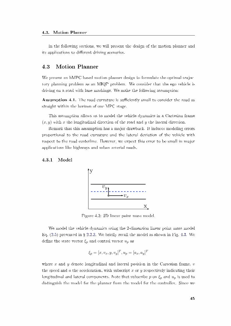
4.3. Motion Planner
In the following sections, we will present the design of the motion planner and
its applications to di�erent driving scenarios.
4.3 Motion Planner
We present an hMPC based motion planner design to formulate the optimal trajec-
tory planning problem as an MIQP problem. We consider that the ego vehicle is
driving on a road with lane markings. We make the following assumption:
Assumption 4.1. The road curvature is su�ciently small to consider the road as
straight within the horizon of one MPC stage.
This assumption allows us to model the vehicle dynamics in a Cartesian frame
(x, y) with x the longitudinal direction of the road and y the lateral direction.
Remark that this assumption has a major drawback. It induces modeling errors
proportional to the road curvature and the lateral deviation of the vehicle with
respect to the road centerline. However, we expect this error to be small in major
applications like highways and urban arterial roads.
4.3.1 Model
x
y
Figure 4.3: 2D linear point mass model.
We model the vehicle dynamics using the 2-dimension linear point mass model
Eq. (2.5) presented in � 2.2.2. We brie�y recall the model as shown in Fig. 4.3. We
de�ne the state vector ξp and control vector up as
ξp = [x, vx, y, vy]T , up = [ax, ay]
T
where x and y denote longitudinal and lateral position in the Cartesian frame, v
the speed and a the acceleration, with subscript x or y respectively indicating their
longitudinal and lateral components. Note that subscribe p on ξp and up is used to
distinguish the model for the planner from the model for the controller. Since we
45

Chapter 4. Model Predictive Control for Autonomous Driving
Integrating Logical Constraints
only consider the planner in this chapter, we omit p in the following paragraph to
simplify the notations. The vehicle dynamics can be compactly written using the
following linear di�erential equation:
ξ =
[A 0
0 A
]ξ +
[B 0
0 B
]u,
A =
[0 0
0 1
], B =
[0
1
].
(4.1)
where 0 is a zero matrix with proper dimensions.
Discretizing the vehicle dynamics with a time step duration of τ leads to the
following equation:
ξk+1 =
[Ad 0
0 Ad
]ξk +
[Bd 0
0 Bd
]uk,
Ad =
[1 τ
0 1
], B =
[12τ
2
τ
].
(4.2)
To take into account the dynamic limitations of the vehicle, bound constraints
are enforced on the state and control signals as
ξ ∈ [ξ, ξ], u ∈ [u, u], (4.3)
with the bounds de�ned as
ξ = [0, 0, y, vy]T , ξ = [+∞, vx, y, vy]T , (4.4a)
u = [ax, ay]T , u = [ax, ay]
T . (4.4b)
We enforce the following condition to couple the longitudinal and the lateral
dynamics
vy ∈ [vx tan(θ), vx tan(θ)]. (4.5)
Remark that this point-mass model is widely used at the planning stage [19, 20]
for normal on-road driving as it is conceptually simple while capturing most of the
vehicle dynamics. In fact, if the constraints (4.3) and (4.5) are properly chosen, we
can reconstruct all vehicle states of a bicycle model using the di�erential �atness
theory [80]. On the other hand, this model is no longer feasible if the vehicle
is operating near its limit, for instance when executing an emergency maneuver.
A common workaround is to design an emergency controller which overrides the
planner in this situation. Here we only consider normal driving situation where the
46

4.3. Motion Planner
point-mass model applies.
4.3.2 From logic propositions to mixed integer constraints
0 20 40 60 80 1005
10
15
20
x(m)
v(m
s)
/
0 20 40 60 80 100−2
0
2
x(m)
y(m)
Speed Limit
Figure 4.4: Illustration of the speed bump scenario with the speed bump regionmarked by gray color.
We �rst recall some basics of propositional logic. We de�ne a literal as an
atomic statement corresponding to a linear mathematical condition on one of the
state variables, for instance: the speed of the vehicle is smaller than 10m/s. Literals
can be combined using connectors, such as ∧ (and), ∨ (or), ¬ (negation); other
connectors like implications (⇒) and equivalences (⇔) can be formed using the
�rst two connectors. To illustrate, we consider a speed bump scenario in which
the vehicle must decelerate to 10m/s on the speed bump situated in the range x ∈[40 m, 60 m] (Fig. 4.4). We de�ne three literals P1 = [xk ≥ 40], P2 = [xk ≤ 60] and
P3 = [vkx ≤ 10]; the rule can then be expressed in the form: ∀k ≥ 0, (P1 ∧P2)⇒ P3,
i.e. if the vehicle's position is within [40 m, 60 m], then the vehicle's longitudinal
speed should be lower than or equal to 10m/s.
Once we have abstracted related logic rules into formal propositions, we can
further reformulate them as a set of linear inequalities with continuous and integer
variables, as shown in [81]. The idea is to force the value of a binary variable to
be equal to 0 (or 1) when a given literal is true, and/or equal to 1 (or 0) when the
literal is false. In the previous example, we can let δki = 1 ⇒ Pi for i ∈ {1, 2, 3} so
47

Chapter 4. Model Predictive Control for Autonomous Driving
Integrating Logical Constraints
that the speed bump rule can be expressed equivalently as, ∀k ≥ 0,
δk1 = 1⇒ xk ≥ 40, (4.6a)
δk2 = 1⇒ xk ≤ 60, (4.6b)
δk3 = 1⇒ vkx ≤ 10, (4.6c)
− δk1 + δk3 ≤ 0, (4.6d)
− δk2 + δk3 ≤ 0, (4.6e)
δk1 + δk2 − δk3 ≤ 1. (4.6f)
The associations (4.6a), (4.6b) and (4.6c) can then be �nally translated to mixed-
integer inequalities using the so-called Big-M method [81]. For instance, (4.6a) is
rewritten as
xk ≥ 40−M(1− δk1 ), (4.7)
where M is a large positive constant. For example, we can conveniently choose M
to be 106.
4.3.3 MPC formulation
We introduce a new vector-valued variable σ such that σk = {0, 1}m is a collection of
all binary variables that are introduced at time k from the reformulation of relevant
literals as mixed-integer linear inequalities. We consider a time horizon T = Kτ with
K being the number of time steps in the prediction horizon. Let ξ = {ξ0, ..., ξK}and u = {u0, ..., uK} respectively be the state and control trajectory for the given
time horizon. Let ξref be the reference trajectory for the vehicle, which can be time-
dependent, state-dependent, or dependent on propositions. Let σ be the trajectory
of the binary variable [σ0, ..., σK ]. We also introduce σref as the reference trajectory
for the binary variables, so that we can also express preferences on some binary states
if needed, for instance to specify a preferred lane in a multi-lane road. At current
time t = 0, we formulate the following optimization problem
minu,σ
J(ξ,u,σ) =
K∑k=0
(||ξk − ξkref ||2Q + ||σk − σkr ||2R + ||uk||2S + ||∆uk||2W ), (4.8)
48

4.3. Motion Planner
subject to
ξ0 = H(ξ), (4.9a)
ξk+1 =
[Ad 0
0 Ad
]ξk +
[Bd 0
0 Bd
]uk, k = 0, ...,K − 1, (4.9b)
ξk ∈ [ξ, ξ], uk ∈ [u, u], k = 0, ...,K, (4.9c)
vky ∈ [vkx tan(θ), vkx tan(θ)], k = 0, ...,K, (4.9d)
∆uk = uk − uk−1, k = 0, ...,K, (4.9e)
C
ξ
ξref
σ
≤ D, (4.9f)
where Q, R, S, and W are non-negative weighting matrices of proper dimensions.
Eq. (4.9a) is the constraint on initial value. We introduce ∆uk as the di�erence
between two consecutive control inputs to penalize jerk (Eq. (4.9e)). Note that
we must know the previous control input u−1. Constraint (4.9f) is the set of all
linear inequalities written in matrix form with two matrices C and D of proper
dimensions, incorporating all mixed-integer constraints derived from the current
context of driving. The cost function (4.8) is quadratic and the constraints (4.9)
are linear and potentially mixed integer. Therefore, the above optimization problem
is an instance of mixed-integer quadratic programming (MIQP) problems. Integer
programming problem are NP-hard and so are MIQP problems since it is a subset
of integer programming problems, however, exact resolution algorithms that deploy
e�cient heuristics are known to solve such problems without exploring the whole
decision tree.
The optimization problem is formulated and solved in a receding horizon fashion.
At each time step, the solution of the problem is a globally optimal trajectory ξ∗pwhich is fed to the tracking controller.
The proposed MPC formulation is su�ciently generic to cover a vast majority
of normal driving scenarios, as will be illustrated in Section 4.4. If we must consider
non-quadratic cost functions, non-linear vehicle dynamics or non-linear constraints,
we can formulate a Mixed Integer Non-linear Program, which, however, is much
harder to solve.
49

Chapter 4. Model Predictive Control for Autonomous Driving
Integrating Logical Constraints
ξ = [0, 0,−2 m,−3 m/s]T , ξ = [free, 25 m/s, 8 m, 3 m/s]T ,u = [−3 m/s2,−1 m/s2]T , u = [3 m/s2, 1 m/s2]T ,
θ = −0.5 rad, θ = 0.5 rad,q1 = 1, q2 = 2, q3 = 4, s1 = 2, s2 = 4, w1 = 4, w2 = 16.
Table 4.1: Parameters used for the hMPC-based motion planner in applicative ex-amples
4.4 Applicative examples and simulations
In this section, we present a variety of applicative examples to concretize the pro-
posed motion planner design. This design can be con�gured to e�ectively handle var-
ious on-road driving scenarios, including speed bump, intersection crossing, obstacle
avoidance, overtaking and lane change. Note that, although the major purpose of
this section is to demonstrate the �exibility of the design, the detailed formulations
for di�erent driving scenarios are by themselves contributions to some challenging
problems for on-road autonomous driving. Simulations are performed with in-depth
quantitative analysis, proving the implementability of our framework.
Throughout this section, we use the following cost function for the planner
J =
K∑k=0
q1(vkx − vref )2 + q2(yk − ykref )2 + q3(vky )2 + s1(akx)2
+ s2(aky)2 + w1(akx − ak−1
x )2 + r2(aky − ak−1y )2,
(4.10)
such that the vehicle tracks a constant desired speed pro�le vref and a potentially
time-varying desired lateral deviation ykref , k ∈ [0, ...,Kp], while trying to minimize
the control e�ort. We do not assume any desired binary state, and therefore the
term ||σk−σkref ||2S in the generic formulation is ignored. In all cases, the ego vehicle
is assumed to start at position (0, 0). Other parameters that are common in all
cases are summarized in Table 4.1. Scenario-speci�c parameters will be presented
respectively in each case study.
In all simulations, we assumed that the perception components estimate the tra-
jectories of surrounding objects using constant velocity hypothesis (objects maintain
constant speeds in the prediction horizon). More realistic estimation methods could
be envisaged but are not considered in this thesis. The vehicle localization is as-
sumed to be perfect.
The motion planner updates at a frequency of 5Hz. The low-level tracking
controller is identical to the one described in � 3.5.
Note that the feasibility issue mentioned in � 2.3.3 also raises in hMPC design, in
which the optimization problem may become infeasible over successive iterations due
50

4.4. Applicative examples and simulations
to small violations of some constraints. The constraint softening technique described
in � 2.3.3 is adopted to transform the concerned constraints to soft constraints. Here
we do not explicitly describe the constraint softening procedure.
We use the commercial solver Gurobi [44] to compute solutions to our MIQP
formulation. Since the MIQP problem is NP-hard and Gurobi uses heavily optimized
heuristics to accelerate calculations, there is no guarantee of computation time (even
though the solver is quite e�cient most of the time). We notice that Gurobi often
�nds the optimal solution in a short time while spending much more time in proving
the optimality of the solution. This inspires us to set an upper-bound of 200ms on
the computation time so that Gurobi returns the currently best solution if hitting
the upperbound. In this way we guarantee the update rate of the motion planner.
However, there is no longer theoretical guarantee of optimality even though we
observe that most of the time the solutions are in fact optimal (while not yet proved
by the solver).
The non-linear optimization problem of the tracking controller is solved by
ACADO Toolkit [43]. Simulation codes are written in C++, and experiments
are performed on a laptop with a mid-range Intel Core i5-5300U CPU clocked at
2.30GHz with 8GB RAM.
4.4.1 Speed bump
Scenario description
The �rst case study considers the speed bump scenario (Fig. 4.4) that is used as an
example in � 4.3.2. The speed bump conditions are given in (4.6). The initial speed
of the vehicle is equal to its desired speed vref = 15 m/s while on the speed bump
(within the interval of [40 m, 60 m]) the maximally allowed speed is 10 m/s.
Simulation results
In the simulation, we use a prediction horizon T = 5 s and time step duration
τ = 0.25 s. Fig. 4.5 illustrates the longitudinal speed pro�le of the planned trajectory
with respect to the traveled distance. We observe that the vehicle e�ectively reduces
its speed to less than 10 m/s.
4.4.2 Intersection crossing
Scenario description
We consider the problem of controlling a vehicle at an intersection, where it is
not allowed to cross the intersection unless no other vehicle (called non-controlled
51

Chapter 4. Model Predictive Control for Autonomous Driving
Integrating Logical Constraints
0 20 40 60 80 1005
10
15
20
x(m)
v(m
s)
/
Predict ion EV
Figure 4.5: Longitudinal speed pro�le with respect to the longitudinal o�set. Greencurves mark the predicted trajectories during the MPC iterations and the blue curvemarks the actual trajectory of the vehicle.
vehicle) is inside the intersecting region. For example, Fig. 4.6 shows a scenario with
two non-controlled vehicles. The ego vehicle has four maneuver choices: crossing
before both cars, after the blue car and before the red car, before the blue car and
after the red car, or after both cars. Some maneuver choices may be impossible or
dynamically infeasible for the ego vehicle. In [82], the authors propose to construct
an MPC problem for each maneuver choice and select the global optimum among
all local optimal solutions. Here, we demonstrate that with our framework explicit
enumeration is no longer necessary.
Ego Vehicle
Veh 1
Veh 2
Figure 4.6: Illustrative example of the intersection crossing scenario. The ego vehicle(white) needs to cross the intersection without colliding with the non-controlledvehicles (red and blue cars). We do not consider road priority in this example.
In our scenario, the initial speeds of three vehicles are set to 10m/s and the
desired speed of the ego vehicle is also set to vref = 10 m/s. We refer the red car as
Vehicle 1 and the blue car as Vehicle 2. The intersection region is set to [52 m, 58 m]
for all vehicles in their local longitudinal coordinate systems. The initial positions
for the ego vehicle, Vehicle 1 and Vehicle 2 are respectively 0, 0 and −30 m.
52

4.4. Applicative examples and simulations
Formulation of constraints
0
25
50
75
100Profile if accelerate
Profile if decelerate
Intersection Region
t(s)
x(m)
Figure 4.7: Illustration of the earliest arrival time and the latest departure time.
Let [L,H] be the path segment of the ego vehicle for the intersection region.
We use o to denote a non-controlled vehicle. The path segment of o inside the
intersecting region is de�ned as [Lo, Ho]. At any given moment, only one vehicle
can be inside the intersection region. Thus if xo ∈ [Lo, Ho], then the ego vehicle
must respect x /∈ [L,H].
At the beginning of a motion planner iteration of the ego vehicle, we monitor
the states of non-controlled vehicles that have not passed their intersection regions.
We �rst compute the earliest arrival time to for o with respect to its intersection
region [Lo, Ho] by assuming that it applies an acceleration of ax,o > 0 (Fig. 4.7):
to = T (Lo − xo, vx,o, ax,o), (4.11)
where T (x, v, a) is a function that computes the time to traverse a distance of x if
the current speed is v and the vehicle applies a constant acceleration of a. If the
vehicle cannot traverse x in �nite time, then the time is set to +∞. The reason of
introducing ax,o instead of assuming constant speed of o is to add a reasonable error
margin on the motion estimation of non-controlled vehicles.
Similarly, we compute the latest departure time to as the latest time instant
when the vehicle leaves the intersection, assuming a constant deceleration ax,o < 0
(Fig. 4.7).
to = T (Ho − xo, vx,o, ax,o). (4.12)
Since the dynamics of the ego vehicle is discretized with a time step duration τ ,
53

Chapter 4. Model Predictive Control for Autonomous Driving
Integrating Logical Constraints
we introduce two integer variables ko and ko as
ko =⌈ toτ
⌉, (4.13a)
ko =⌊ toτ
⌋, (4.13b)
We formulate the safety constraints for the ego vehicle. For each non-controlled
vehicle, we introduce a binary variable δo ∈ {0, 1}. The planner of the ego vehicle
runs with a horizon K, if ko ≤ ko ≤ K, we let
δo = 0⇒ xko ≥ H, (4.14a)
δo = 1⇒ xko ≤ L. (4.14b)
As the variable δo can only take either 0 or 1 for its value, the ego vehicle is
required to either traverse the intersection before o's earliest arrival time or stay out
of the intersection until o leaves the intersection.
If ko ≤ K ≤ ko, we let
δo = 0⇒ xko ≥ H, (4.15a)
δo = 1⇒ xK ≤ L. (4.15b)
The ego vehicle is required to either cross the intersection before o's earliest arrival
time or stay out of the intersection at the end of the prediction horizon.
If K ≤ ko ≤ ko , o is still far from intersection, thus we do not add any constraint
on the ego vehicle.
Eq. (4.14) - Eq. (4.15) are then integrated to the hybrid MPC framework fol-
lowing the procedure of � 4.3.3.
Note that ax,o and ax,o are two design parameters that can be chosen according
to the required level of conservativeness: choosing large absolute values increases
the conservativeness of the motion planner.
Simulation results
In simulations, we use a prediction horizon T = 5 s and τ = 0.25 s. We choose
ax,o = 1 m/s2 and ax,o = −1 m/s2. In the �rst simulation, we assume that non-
controlled vehicles keep constant speed during the intersection crossing. In Fig. 4.8a,
we observe that the ego vehicle choose to traverse the intersection after Vehicle 1
54

4.4. Applicative examples and simulations
0 2 4 6 8 100
25
50
75
100
t(s)
x(m
)
EV Veh 1 Veh 2
(a)
0 2 4 6 8 1005101520
t(s)
v(m
s)
/
Predict ion EV
(b)
Figure 4.8: Intersection simulation 1: (a) Longitudinal positions of three vehiclesas functions of time. (b) Longitudinal speed pro�le of the ego vehicle as well as thepredicted trajectories during MPC iterations. EV - Ego Vehicle, Veh 1 - Vehicle 1,Veh 2 - Vehicle 2.
and before Vehicle 2. Fig. 4.8b illustrates the speed pro�le of the ego vehicle. We
observe that the ego vehicle slightly decelerates at the beginning to yield to Vehicle
1 and then return to its desired speed.
To serve as a comparison, we perform a second simulation in which we force
Vehicle 2 to accelerate with an acceleration of 1 m/s2 between t = 2.5 s and t = 10 s.
Fig. 4.9a illustrates the result. The ego vehicle chooses to yield to both Vehicle 1
and Vehicle 2. In Fig. 4.9b, the predicted trajectories suggest that during the �rst
2.5 s, the ego vehicle decides to pass between Vehicle 1 and Vehicle 2. However,
since Vehicle 2 starts to accelerate from 2.5 s, the motion planner �nds that this
decision is no longer optimal and switches to another decision.
Note that the proposed formulation can also be adapted to select the optimal
55

Chapter 4. Model Predictive Control for Autonomous Driving
Integrating Logical Constraints
0 2 4 6 8 100
25
50
75
100
t(s)
x(m
)
EV Veh 1 Veh 2
(a)
0 2 4 6 8 1005101520
t(s)
v(m
s)
/
Predict ion EV
(b)
Figure 4.9: Intersection simulation 2: (a) Longitudinal positions of three vehiclesas functions of time. (b) Longitudinal speed pro�le of the ego vehicle as well as thepredicted trajectories during MPC iterations. EV - Ego Vehicle, Veh 1 - Vehicle 1,Veh 2 - Vehicle 2.
time to enter a highway in a merging scenario and compute the associated trajectory.
56

4.4. Applicative examples and simulations
4.4.3 Obstacle avoidance
Scenario description
0 50 100 150 200−2
0
2
x(m)
y(m)
Figure 4.10: Illustration of the obstacle avoidance scenario. The obstacle is coloredin red. The light-red area is used to take into account the size of the ego vehicle.
We now consider an obstacle avoidance scenario during on-road driving as shown
in Fig. 4.10. There are two identical obstacles centered at (60, 1) and (120,−1). The
irregular shapes of obstacles are approximated using minimal bounding rectangles
(region with light red color) with the length Lo = 10 m and width Wo = 2.6 m,
taking into account the size of the ego vehicle. A more complex convex polygonal
modeling is also possible, at the cost of increased computational complexity.
Formulation of constraints
For an obstacle o with bounding rectangle [xko − Lo, xko + Lo]× [yko −Wo, yko +W k
o ],
the set of constraints for collision avoidance is then given as ∀k ≥ 0,
δko,1 = 1⇒ x(k) ≤ xko − Lo, (4.16a)
δko,2 = 1⇒ x(k) ≥ xko + Lo, (4.16b)
δko,3 = 1⇒ x(k) ≤ yko −Wo, (4.16c)
δko,4 = 1⇒ x(k) ≥ yko +Wo, (4.16d)
δko,1 + δko,2 + δko,3 + δko,4 = 1. (4.16e)
Note that the formulation allows both moving and still obstacles. The condi-
tions (4.16) state that the vehicle must be separated from the obstacle, either by a
longitudinal distance Lo or laterally by Wo.
Simulation results
We choose the horizon of the motion planner as T = 10 s and τ = 0.5 s. Fig. 4.11a
illustrates the vehicle trajectory. We notice that the vehicle successfully avoids all
obstacles. Fig. 4.11b shows the vehicle speed and the steering angle pro�les.
57

Chapter 4. Model Predictive Control for Autonomous Driving
Integrating Logical Constraints
0 50 100 150 200−2
0
2
x(m)y(m)
Predict ion EV
(a)
0 5 10 15 205
10
15
20
t(s)
v(m/s)
0 5 10 15 20−2
0
2·10−2
φ(rad)
v φ
(b)
Figure 4.11: Obstacle avoidance scenario: (a) Vehicle trajectory as well as predictedtrajectories. (b) Speed pro�le and steering angle pro�le.
4.4.4 Overtaking in a two-lane road
Scenario description
−100 0 100 200 300 400
0
4
x(m)
y(m)
Ego Vehicle
Figure 4.12: Illustration of the overtaking scenario.
We consider an overtaking scenario on a two-lane road with oncoming tra�c
as in Fig. 4.12. The ego vehicle is driven towards the east with a slow vehicle in
the front. Two vehicles are on the adjacent lane driving on the opposite direction.
The ego vehicle has multiple choices for overtaking: overtaking before the arrival of
the two oncoming vehicles, overtaking using the space between the two vehicles or
overtaking after the passing of two vehicles. This scenario is considered as di�cult
for both human drivers and autonomous vehicles [83, 20, 2].
We assume that the initial speed of non-controlled vehicles are 10m/s and the
initial speed of the ego vehicle is equal to its desired speed vref = 15 m/s. Vehicles
are all 3.5 m and 2.5 m wide.
58

4.4. Applicative examples and simulations
Formulation of constraints
It is possible to model surrounding vehicles as rectangles as in the previous case
study, thus requiring four integer variables for each vehicle and each time step k.
However, by introducing the so called ramp barrier [20, 83], the problem can be
further simpli�ed by approximating the rectangular obstacle region by a triangular
one only requiring two integer variables as shown in Fig. 4.12.
Consider a surrounding vehicle o; if o is on the same lane as the ego vehicle, the
constraints are given as
δko = 0⇒ −xk − xkoLo
+yk − ykoWo
≥ 1, (4.17a)
δko = 1⇒ xk − xkoLo
+yk − ykoWo
≥ 1, (4.17b)
where Lo and Wo are minimal longitudinal and lateral separations during lane
change. Similarly, the constraints for an oncoming vehicle o can be modeled as
δko = 0⇒ xk − xkoLo
+yk − ykoWo
≤ −1, (4.18a)
δko = 1⇒ −xk − xkoLo
+yk − ykoWo
≤ −1, (4.18b)
Simulation results
In simulations, we adopt a su�ciently long prediction horizon of T = 15 s so that the
planner can plan a complete overtaking trajectory. We let τ = 0.5 s. The parameters
Lo = 8 and Wo = 3.5.
In the �rst simulation, we assume that all surrounding vehicles drive at constant
speeds. The duration of simulation is 30 s. Fig. 4.13a illustrates the overtaking
trajectory. In Fig. 4.13b, we observe that the ego vehicle �rst decelerates slightly to
wait the �rst on-coming vehicle to pass, then it accelerates to use the space between
the �rst and the second on-coming vehicles to perform the overtaking.
To serve as a comparison, in the second simulation, we assume that the second
on-coming vehicle accelerates with a constant acceleration of 1 m/s2 between t =
7.5 s and t = 15 s and maintains constant speed for the rest of time. Fig. 4.14a
illustrates the trajectory of overtaking. The ego vehicle �rst plans the same strategy
as in scenario 1, by using the space between two oncoming vehicles to overtake.
However, as the second on-coming vehicle starts to accelerate, the ego vehicle �nds
that it's more desirable to wait for both on-coming vehicles to pass and then perform
59

Chapter 4. Model Predictive Control for Autonomous Driving
Integrating Logical Constraints
the overtaking. This scenario demonstrates the reactivity of the motion planner with
respect to the changes of surrounding vehicles.
−100 0 100 200 300 400
0
4
8
x(m)
y(m)
Predict ion EV
012345 012345
0 1 2 3 4 50 1
2
34 5
(a)
0 5 10 15 20 25 305
10
15
20
25
t(s)
v(m/s)
0 5 10 15 20 25 30−2
0
2·10−2
φ(rad)
v φ
(b)
Figure 4.13: Overtaking simulation 1: (a) the trajectory of overtaking as well asthe predicted trajectories. We mark the positions of vehicles at six di�erent timeinstants using natural numbers and color codes (lighter color means further timeinstant). (b) Speed and steering pro�les.
60

4.4. Applicative examples and simulations
−100 0 100 200 300 400
0
4
8
x(m)
y(m)
Predict ion EV
0 1
23 4
50 1 2 3 4 5
012345 012345
(a)
0 5 10 15 20 25 305
10
15
20
25
t(s)
v(m/s)
0 5 10 15 20 25 30−2
0
2·10−2
φ(rad)
v φ
(b)
Figure 4.14: Overtaking simulation 2: (a) the trajectory of overtaking as well as thepredicted trajectories, (b) speed and steering pro�les.
61

Chapter 4. Model Predictive Control for Autonomous Driving
Integrating Logical Constraints
4.4.5 Lane change
Scenario description
−100 0 100 200 300 400 500 600
0
4
8
12
x(m)
y(m)
Ego Vehicle
Figure 4.15: Illustration of the lane change scenario
The �nal scenario considers the problem of decision making and motion planning
for a lane change maneuver: the ego vehicle must decide the objective lane as well
as the optimal trajectory to reach this lane, without colliding with surrounding
vehicles.
Fig. 4.15 shows a highway with three lanes. The ego vehicle starts in the right-
most lane with a speed of 20 m/s, equal to its desired speed. Surrounding vehicles
are distributed over three lanes. The vehicle on the leftmost lane drives at a speed
of 20 m/s while other surrounding vehicles drive at a speed of 15 m/s. Vehicles are
all 3.5 m and 2.5 m width. Since the ego vehicle will soon catch up with the slow
vehicle in the front, it either needs to decelerate to synchronize its speed with the
front vehicle, or changes lane.
Formulation of constraints
The complexity of this problem lies in the multiple discrete choices raised from
multiple lanes and multiple vehicles on each lane. References [79, 78] have considered
this problem using MILP formulations; however, their modeling cannot ensure that
trajectories are dynamically feasible due to important simpli�cations of the vehicle
dynamics.
We consider a road with N lanes, labeled by γ ∈ {1, ..., N}. We introduce a
binary variable δkγ that equals 1 if the ego vehicle is on lane γ at time step k. Let I
be the label set of surrounding vehicles and Iγ be the set of vehicles inside lane γ.
Let yγ be the centerline of the lane γ and ykr be the reference lateral deviation at
time step k. We introduce the following logical constraint: ∀k > 0,
δkγ = 1⇒(ykr = yγ ∧ yk ∈ [y
γ, yγ ]
), (4.19)
62

4.4. Applicative examples and simulations
such that, if the ego vehicle is in lane γ, then the vehicle should be within the
boundary of lane γ and the reference lateral deviation should be set to the centerline
of the lane.
Moreover, we add the following collision avoidance constraints: ∀k ≥ 0,
δkγ = 1⇒ ∀i ∈ Iγ ,δko = 0⇒ xk ≤ xko − Lo,δko = 1⇒ xk ≥ xko + Lo,
(4.20)
such that the ego vehicle must avoid collisions with all the vehicles in lane γ.
The ego vehicle is only allowed to be in one lane at any given time, thus we add
the following constraint:∀k ≥ 0,N∑γ=1
δkγ = 1 (4.21)
Constraints (4.19), (4.20) and (4.21) are enforced along with constraints on ve-
hicle dynamics on the formulated MIQP problem.
Remark that this formulation considers the vehicle as a point mass. It is thus
necessary to have enough safety margin on Lo to take into account the shape of the
vehicle.
Simulation results
The horizon is set to T = 15 s and the time step τ = 0.5 s. The simulation duration
is 30 s. The parameter Lo is chosen to be 10 m. We observe in Fig. 4.16a that the
ego vehicle chooses the left-most lane as the objective lane since only in this lane
the ego vehicle can drive at its desired speed. It plans dynamically feasible and
collision-free trajectories to reach the lane within the prediction horizon.
63

Chapter 4. Model Predictive Control for Autonomous Driving
Integrating Logical Constraints
−100 0 100 200 300 400 500 600
0
4
8
12
x(m)
y(m)
Predict ion EV
01
2
3 4 5
0 1 2 3 4 5
0 1 2 3 4 50 1 2 3 4 5
0 1 2 3 4 5
(a)
0 5 10 15 20 25 305
10
15
20
25
t(s)
v(m/s)
0 5 10 15 20 25 30−1
0
1·10−2
φ(rad)
v φ
(b)
Figure 4.16: Lane change scenario: (a) The trajectory of lane change as well aspredicted trajectories. We mark the positions of vehicles at six di�erent time instantsusing natural numbers and color codes (lighter color means further time instant).(b) Speed and steering pro�les.
64

4.5. Experiment
Computation time
The execution time statistics for the hMPC based motion planner are summarized in
Fig 4.17. We observe that the motion planner is able to compute optimal trajectories
within 100ms for the scenarios of speed bump, intersection crossing and obstacle
avoidance. For the scenarios of overtaking and lane change, the computation times
for the �rst 15 s hit regularly the upper-bound of 200ms. The reason is two-fold:
�rst, the number of time steps for both scenarios is 30, which leads to a large number
of continuous and discrete variables; second, there are many maneuver variants in
both scenarios.
0 5 10 15 20 25 300
50
100
150
200
250
t(s)
Comp.Tim
e(m
s)
SB IC Sim. 1 OBS OT Sim. 1 LC
Figure 4.17: Statistics of computation time for di�erent simulations
4.5 Experiment
Setup
The experiment has been performed with the Mercedes-Benz S-Class S 500 vehi-
cle Bertha of Karlsruhe Institute of Technology at a test ground near the campus.
Bertha weights 1900 kg and is equipped with a 195 kW diesel engine. It is equipped
with a state-of-the-art computer powered by Intel Xeon 16-core 2.6GHz CPU. The
computer runs Robot Operating System (ROS) on the top of a Ubuntu linux. It
uses a high precision OxTS RT3000 INS GPS to perform centimeter-level localiza-
tion. Mercedes-Benz has provided a well-de�ned interface to retrieve information
on vehicle states and to control acceleration and steering. The hMPC-based motion
planner was implemented as a ROS package and was integrated into the existing
architecture of the vehicle. Note that unlike in simulations, we use the low-level
controller shipped with the vehicle for trajectory tracking.
Due to the limit of the test ground and in order to test the applicability of the
planner on curvy roads, we have designed a circular road with a radius of 30m
65

Chapter 4. Model Predictive Control for Autonomous Driving
Integrating Logical Constraints
for the inner lane and a radius of 34m for the outer lane. The tra�c direction
of the inner lane is clock-wise while the outer lane is counter clock-wise. We have
designed a scenario similar to the overtaking example in � 4.4.4, with one simulated
vehicle running (clock-wise) on the inner lane at a constant speed of 2m/s and two
simulated vehicles running (counter clock-wise) on the outer lane at a constant speed
of 3m/s. The desired speed of the ego vehicle as well as its initial speed is set to
5m/s. The goal of this experiment is to observe if the motion planner can work in
real world and plan dynamically feasible trajectories for overtaking.
Results
We have successfully performed multiple �eld tests. Fig. 4.18a demonstrates the
trajectory of the ego vehicle as well as the predicted trajectories in one of the tests.
We observe that the vehicle successfully performed the overtaking using the space
between two on-coming vehicles. Fig. 4.18b shows the speed and the steering pro�les
of the ego vehicle. Note that there is a large steering input at around t = 24 s, which
is caused by the instability of the default tracking controller at low speeds.
4.6 Concluding remarks
We have presented a hybrid MPC design of motion planner for the on-road au-
tonomous driving in normal conditions. Numerous applicative examples are pro-
vided to show the �exibility of the proposed design in handling challenging situa-
tions. Field experiments have also been performed to verify the real-world applica-
bility of the design.
66

4.6. Concluding remarks
−40 −20 0 20 40−40
−20
0
20
40
x(m)
y(m)
Predict ion EV
0
12
3
0
1
2
3
0
1
2
3
0
1 2
3
4
5
4
5
4
5
4
5
(a)
0 10 20 30 400
2
4
6
t(s)
v(m/s)
0−0.4
−0.2
0
φ(rad)
v φ
(b)
Figure 4.18: Experiments: (a) The trajectory of overtaking as well as the predictedtrajectories. We mark the positions of vehicles at six di�erent time instants usingnatural numbers and color codes (lighter color means further time instant).(b) Thespeed pro�le and the steering pro�le.
67


Chapter 5
Control Framework for Convoy
In the previous two chapters, we have considered the control framework for individ-
ual vehicles. We have employed MPC based techniques to plan collision-free and
optimal trajectories for autonomous vehicles and to track reference trajectories.
In this chapter, we will consider the cooperative formation control of multiple
autonomous vehicles in an on-road environment. We will present a hierarchical
framework that employs MPC based approaches as building blocks. The framework
uses a global convoy supervisor to manage the formation and local vehicle controllers
to track the formation-keeping reference trajectories satisfying various constraints
of the vehicles. The reference trajectories of a vehicle are computed from its leader's
trajectories, based on a pre-de�ned formation tree. The proposed framework will
be validated using high-�delity simulations.
5.1 Introduction
Cooperative strategies for groups of autonomous vehicles start to attract atten-
tions from both automotive industry and research institutions, due to their poten-
tial in improving tra�c e�ciency and reducing road accidents. Previous projects
(PATH [22], Cybercars-2 [23], CHAUFFER I & II [28] and SARTRE [29]) have
extensively studied a special form of cooperative driving: platoon, in which a group
of vehicles forms a linear formation. It is shown that platooning vehicles brings a
15% to 30% fuel consumption reduction and a 3 to 5 times increase of road through-
put [30].
In this chapter, we consider an extended version of platoon in which multiple
vehicles can enter a formation (also referred to as convoy) with both longitudinal
and lateral separations (e.g. Fig. 5.1). We expect that this extension can �nd its
applications in cooperative tasks, for instance protecting a VIP vehicle, snowplowing
(see example in [84]), cooperative lane change, etc..
In the robotic and control community, generic formation control problem for mul-
tiple robots has been an active research area for decades. Roughly speaking, there
are three approaches to tackle this problem, namely leader-following, virtual struc-
ture and behavioral approaches. In leader-following approaches [85, 86], a leader is

Chapter 5. Control Framework for Convoy
V0
V1
V2
s
obs
r
Figure 5.1: A three-vehicle formation with an obstacle on the road.
selected to track a reference trajectory, while other robots maintain a relative ori-
entations/position o�sets from the leader. The virtual structure approach [87, 88]
considers the formation as a rigid structure. Robots are regarded as nodes in a
structure: a trajectory of the structure is �rst calculated and then transformed to
the reference trajectories of individual robots. In behavioral approaches [89], robots
are prescribed with several behaviors, notably goal seeking, local formation keeping,
collision avoidance, etc. The control of each individual robot is a weighted aver-
age of the control for each behavior. The global group behavior emerges from the
behaviors of individual vehicles.
The literature in robot formation control lays a solid foundation for the formation
keeping problem of multiple autonomous vehicles. However, unique challenges exist
to apply them to on-road driving. Firstly, vehicles are constrained to move in a
highly structured environment. Thus the formation must adapt to the road shape.
Secondly, each individual vehicle as well as the entire convoy must respect tra�c
rules and avoid collisions with other tra�c participants and other convoy members.
Thirdly, convoys must be �exible so that we can recon�gure them if necessary.
There exists some previous work that tackles the formation keeping problem of
autonomous vehicles on the road. Kato et al. [31] consider a speci�c convoy problem
with 5 vehicles spreading over two lanes using a leader-following approach. In [30],
a distributed graph-based convoy control algorithm is proposed. Each vehicle mem-
orizes and tracks its neighborhood. The local control input is calculated using the
Laplacian graph method. The advantage of this method is that it is fully decen-
tralized. However, the formation is limited to a rectangle shape and the vehicle
controller is in its simplest form (feedback controller based on �rst order modeling
of the vehicle, no obstacle avoidance capability, etc.). None of the above mentioned
work satis�es the requirements on intra-formation collision avoidance and convoy
recon�guration.
We propose and validate a novel on-road convoy control framework based on the
leader-following approach, upon which we propose multiple adaptations to handle
the challenges raised by the on-road driving setting. We adopt a hierarchical design,
composed of a global convoy supervisor and multiple local vehicle controllers. The
70
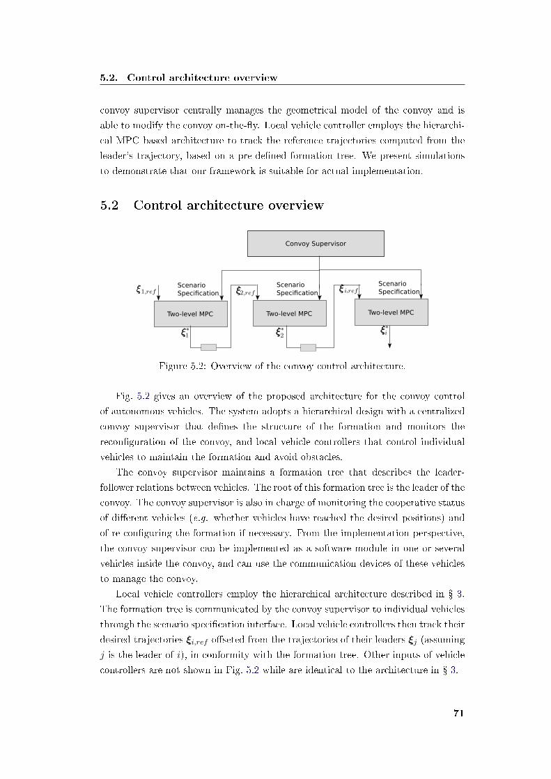
5.2. Control architecture overview
convoy supervisor centrally manages the geometrical model of the convoy and is
able to modify the convoy on-the-�y. Local vehicle controller employs the hierarchi-
cal MPC based architecture to track the reference trajectories computed from the
leader's trajectory, based on a pre-de�ned formation tree. We present simulations
to demonstrate that our framework is suitable for actual implementation.
5.2 Control architecture overview
Two-level MPC
Convoy Supervisor
Scenario Specification
Two-level MPC
Scenario Specification
Two-level MPC
Scenario Specification
Figure 5.2: Overview of the convoy control architecture.
Fig. 5.2 gives an overview of the proposed architecture for the convoy control
of autonomous vehicles. The system adopts a hierarchical design with a centralized
convoy supervisor that de�nes the structure of the formation and monitors the
recon�guration of the convoy, and local vehicle controllers that control individual
vehicles to maintain the formation and avoid obstacles.
The convoy supervisor maintains a formation tree that describes the leader-
follower relations between vehicles. The root of this formation tree is the leader of the
convoy. The convoy supervisor is also in charge of monitoring the cooperative status
of di�erent vehicles (e.g. whether vehicles have reached the desired positions) and
of re-con�guring the formation if necessary. From the implementation perspective,
the convoy supervisor can be implemented as a software module in one or several
vehicles inside the convoy, and can use the communication devices of these vehicles
to manage the convoy.
Local vehicle controllers employ the hierarchical architecture described in � 3.
The formation tree is communicated by the convoy supervisor to individual vehicles
through the scenario speci�cation interface. Local vehicle controllers then track their
desired trajectories ξi,ref o�seted from the trajectories of their leaders ξj (assuming
j is the leader of i), in conformity with the formation tree. Other inputs of vehicle
controllers are not shown in Fig. 5.2 while are identical to the architecture in � 3.
71

Chapter 5. Control Framework for Convoy
In the following, we will detail the design for the convoy control architecture.
5.3 Convoy supervisor
In this section, we will present in detail the design of the convoy supervisor. � 5.3.1
will discuss the mathematical representation of the convoy. � 5.3.2 will consider the
strategy that allow vehicles in a convoy to avoid collisions with each other. � 5.3.3
will investigate the mechanism for safe modi�cations of convoy structures.
5.3.1 Convoy model
We consider the convoy in a road-following coordinate system. We assume that the
centerline of a lane γ ∈ R2 is selected as the reference curve to de�ne the Frenet
coordinate system (s, r), where s is the curvilinear abscissa along γ, and r the lateral
deviation.
We consider a set N = {0, .., N} of N + 1 vehicles, in which we arbitrarily use
0 as leader; the leader is considered to be a physical vehicle for simplicity in this
thesis, while it could also be a virtual reference point.
Formation tree
To describe the interdependence relations between vehicles in the formation, we
de�ne a formation tree as a directed tree G = (N , E), whose nodes are the vehicles
of N and with a set of edges E such that the root node is the leader 0. Such a tree
can be represented as an adjacency matrix (gij) of size (N + 1)× (N + 1), in which
element gij equals 1 if the edge i→ j is in E , and 0 otherwise.
Example 5.1. Consider a triangular formation of the three vehicles as shown in
Fig. 5.1. The formation tree G is given as:
0 1 20 0 0 0
1 1 0 0
2 0 1 0
such that vehicle 1 computes its formation control trajectory relative to vehicle 0,
and vehicle 2 computes its trajectory relative to vehicle 1.
We de�ne the target shape of the formation through a (N + 1)× 2 matrixM in
which each row vector (sdi , rdi ) encodes the target position of vehicle i relatively to
vehicle 0.
72

5.3. Convoy supervisor
Example 5.2. Assuming that the convoy in Fig. 5.1 is coordinated both longitu-
dinally and laterally, the matrixM is given as:
sdi rdi0 0 0
1 −10 3
2 −10 −3
5.3.2 Intra-convoy collision avoidance
sr
Figure 5.3: Road space partitioning with respect to vehicle i.
Our aim is to design an intra-formation collision avoidance strategy such that
vehicles will neither collide in normal on-road driving situations, nor in situations
where the formation is perturbed by obstacles.
Remark that the exact rectangle-shaped safety region of a vehicle is non-di�erentiable,
and multiple maneuver choices exist for collision avoidance. For instance, consider
a 2-vehicle scenario (e.g., vehicles 1 and 2 in Fig. 5.1): if vehicle 1 approaches ve-
hicle 2, vehicle 2 has four strategies to avoid collision: accelerate to the front of
vehicle 1, decelerate behind vehicle 1, move further to the right or circumvent vehi-
cle 1 from its left. The problem becomes exponentially complex as the number of
vehicles increases due to its combinatorial nature. In [90], a similar problem is han-
dled through the formulation of a mixed integer programming problem, in which
the avoidance decisions are modeled as binary variables. However, the real-time
requirement of our algorithm stops us from adopting the same method.
Here, we adopt a hybrid modeling approach. Let us de�ne an ordered priority
list L as a permutation of {0, 1, ..., N}, representing the relative priorities between
vehicles. With a slight abuse of notation, we let L(i) be the rank of i in L, i.e.L(i) = j if, and only if, i is the j-th element of L. We enforce the following
constraint for any pair of vehicles i, j ∈ N :
Design constraint: L(i) < L(j) ⇐⇒ sdi ≥ sdj
73

Chapter 5. Control Framework for Convoy
Under this constraint, the list L encodes a tra�c rule for the formation of vehi-
cles: each vehicle is only responsible for avoiding collisions with the higher-priority
vehicles on the road, i.e with its predecessors in L.We divide the space outside the collision region into six areas: for a vehicle i,
we partition the space using three a�ne functions h1i (s, r) = 0, h2
i (s, r) = 0 and
h3i (s, r) = 0 as shown in Fig. 5.3:
h1i (s, r) = −r − ri
∆r+s− si
∆s+ 1, (5.1a)
h2i (s, r) =
r − ri∆r
+s− si
∆s− 1, (5.1b)
h3i (s, r) =
s− si∆s
+ 1. (5.1c)
where ∆s and ∆r are geometric parameters described in Fig. 5.3. For each vehicle
i, these a�ne functions de�ne a partition of the (s, r) plane in six sub-spaces labeled
as Ami ,m ∈ {0, ..., 5} as shown in Fig. 5.3. By de�nition, vehicle i is always inside
region A0i , and we enforce safety by preventing vehicles with lower priority than i
from entering A0i . In what follows, we call A0
i the protected region for i, and the
union of subsets Ami ,m ∈ {1 . . . 5} forms the safe region with respect to i.
For an arbitrary vehicle j, the following logic rule is introduced for all i ∈ N :
L(i) < L(j)⇒ (sj , rj) ∈⋃
m={1,...,5}Ami . (5.2)
Rule (5.2) e�ectively forces each vehicle to remain in the safe region with respect
to the vehicles having higher priority in L. In a classic hybrid MPC setting, a binary
decision variable would be required to select in which subspaces Ami ,m ∈ {1, . . . , 5}vehicle j should be. In this chapter we adopt a di�erent, simpler approach consisting
of using the shape matrix M to implicitly constrain the choice of the maneuver
choices as follows: ∀i, j ∈ N such that L(i) < L(j),(sdji ≥ −∆s ∧ rdji > 0
)⇒ h1
i (sj , rj) ≤ 0, (5.3a)(sdji ≥ −∆s ∧ rdji < 0
)⇒ h2
i (sj , rj) ≤ 0, (5.3b)
sdji < −∆s⇒ h3i (sj , rj) ≤ 0. (5.3c)
where sdji = sdj − sdi and rdji = rdj − rdi are the target relative position of vehicle j
from vehicle i in the convoy.
The above constraints de�nes a subspace of⋃m={1...5}A
mi . They are linear (and
therefore di�erentiable).
74

5.3. Convoy supervisor
Example 5.3. Let L = {0, 1, 2} be the priority list for the formation illustrated in
Fig. 5.1. The constraint for vehicle 1 can be computed from (5.3) as h30(s1, r1) ≤ 0
such that the safe region (relative to vehicle 0) is A20 ∪A3
0 ∪A40, forcing vehicle 1 to
stay behind vehicle 0. The constraint for vehicle 2 is h30(s2, r2) ≤ 0∧ h2
1(s2, r2) ≤ 0,
such that vehicle 2's safe region is (A20 ∪A3
0 ∪A40) ∩ (A3
1 ∪A41 ∪A5
1): vehicle 2 must
stay behind vehicle 0, and stay on the right-hand or behind vehicle 1.
5.3.3 Dynamic formation modi�cation
We consider the recon�guration of convoy structure during cooperative autonomous
driving. Let G be a formation tree, M a shape matrix and L a priority list, all
compatible with respect to the design constraint: we denote by F = (G,M,L) the
corresponding formation. We give the following de�nition:
De�nition 5.1 (Isormorphic formation). Two formations F1, F2 are said to be
isomorphic if L1 = L2.
In this chapter, we only consider isomorphic formation changes: the recon�gura-
tion ofM and/or G. Non-isomorphic formation changes that involve the modi�ca-
tion of L are not considered in this thesis. The recon�guration of G only a�ects the
behaviors of vehicles when the formation is perturbed. Thus we are free to modify
G as long as the tree structure covers all nodes. On the other hand, we cannot ar-
bitrarily modify the shape matrixM due to the design of intra-formation collision
avoidance constraint (5.3). Consider the case of two vehicles i, j with L(i) < L(j),
where vehicle j is in the partition A5i of vehicle i. Assuming that we recon�gure the
shape matrix, if the new goal con�guration of vehicle j resides in A4i , then vehicle j
can plan a trajectory to its goal con�guration because both A4i and A
5i belong to the
constraint h2i (s, r) ≤ 0. However, if the goal con�guration is in A2
i , vehicle i can-
not plan a feasible trajectory under the current formulation as A2i is not a feasible
region under the current constraint h21. It is necessary to set an intermediate goal
con�guration at A3i . Once vehicle j reaches A3
i , the collision avoidance constraint
must be switched from h2i to h3
i and then vehicle j can continue to move towards
its goal con�guration. This issue is a side e�ect of the space partitioning technique.
We propose the following de�nitions:
De�nition 5.2 (1-step Reachable Element). Consider two elements of the partition
Ami and Ani ; we say Ani is 1-step reachable from Ami if there exists l ∈ {1, 2, 3} such
that hli ≤ 0 over Ani ∪Ami .
This means we need at least one of the rules (5.3) to be kept during recon�gu-
ration. We can see that A1i is reachable from A2
i and A3i ; A
2i is reachable from A1
i ,
75

Chapter 5. Control Framework for Convoy
0
1 2
3
0
1
2
3
0
12
3
0 1
2 3
Figure 5.4: A sequence of 1-step reachable isomorphic transformations.
A3i and A
4i ; A
3i is reachable from all elements except A0
i ; and symmetrically for the
other areas.
De�nition 5.3 (1-step Reachable Formation). Consider two formations M1 and
M2. We say that M2 is 1-step reachable from M1 if ∀i, j ∈ N such that L(i) <
L(j), the con�guration of vehicle j with respect to vehicle i inM2 is 1-step reachable
fromM1.
Theorem 5.1. Consider an arbitrary pair of isomorphic formations F1, F2, we can
transform from F1 to F2 through a �nite sequence of 1-step reachable formations.
The proof is intuitive, since A3i is reachable from all elements except A0
i . There-
fore, any formation can be transformed to a linear formation in a �nite number of
steps. With the above theoretical result, in order to recon�gure the formation to
the desired one, we only need to design an intermediate sequence of 1-step reachable
formations. Then we can set up a discrete supervisor to control the transformation.
Example 5.4. We consider a formation of four vehicles. Fig. 5.4 illustrates a
sequence of 1-step reachable isomorphic transformations. The corresponding shape
matrices are given as follows.
M1 M2 M3 M40 0
−10 3
−10 −3
−20 0
0 0
−10 0
−20 0
−30 0
0 0
−10 −3
−10 3
−20 0
0 3
0 −3
−10 3
−10 −3
5.4 Local vehicle controller
We employ the same vehicle controller as described in � 3, with adaptations at the
motion planner level to take into account cooperative constraints.
76
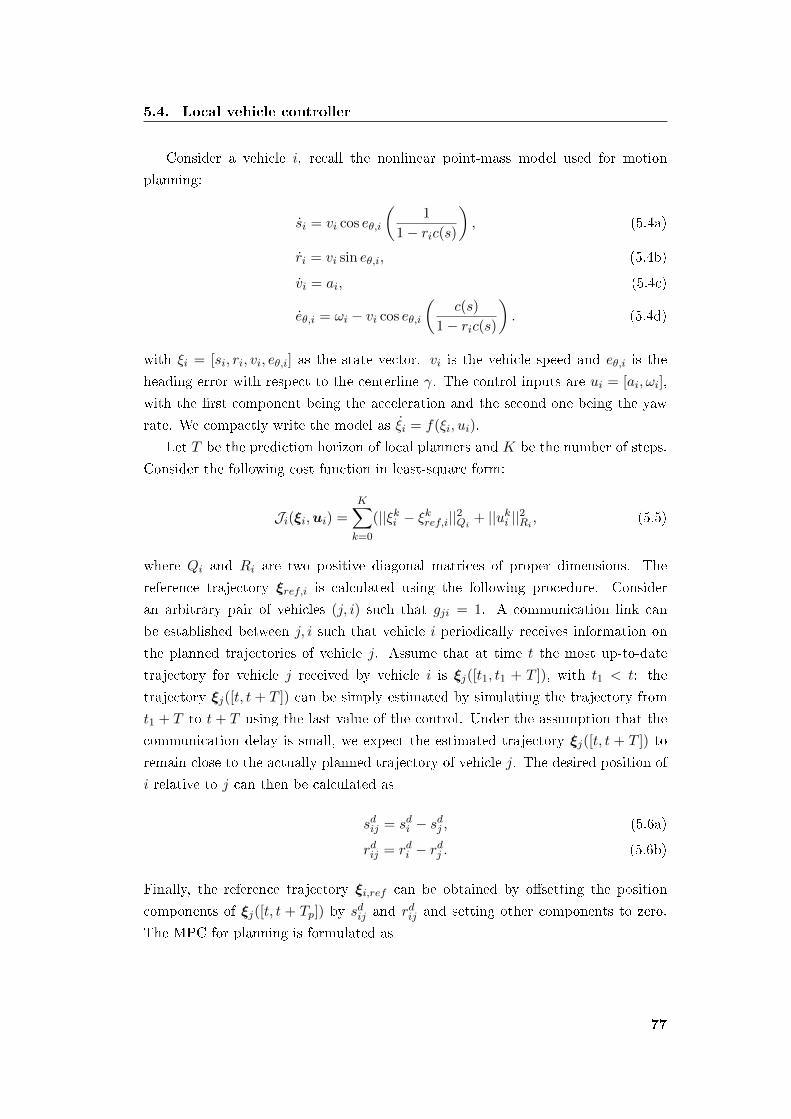
5.4. Local vehicle controller
Consider a vehicle i, recall the nonlinear point-mass model used for motion
planning:
si = vi cos eθ,i
(1
1− ric(s)
), (5.4a)
ri = vi sin eθ,i, (5.4b)
vi = ai, (5.4c)
eθ,i = ωi − vi cos eθ,i
(c(s)
1− ric(s)
). (5.4d)
with ξi = [si, ri, vi, eθ,i] as the state vector. vi is the vehicle speed and eθ,i is the
heading error with respect to the centerline γ. The control inputs are ui = [ai, ωi],
with the �rst component being the acceleration and the second one being the yaw
rate. We compactly write the model as ξi = f(ξi, ui).
Let T be the prediction horizon of local planners and K be the number of steps.
Consider the following cost function in least-square form:
Ji(ξi,ui) =K∑k=0
(||ξki − ξkref,i||2Qi+ ||uki ||2Ri
, (5.5)
where Qi and Ri are two positive diagonal matrices of proper dimensions. The
reference trajectory ξref,i is calculated using the following procedure. Consider
an arbitrary pair of vehicles (j, i) such that gji = 1. A communication link can
be established between j, i such that vehicle i periodically receives information on
the planned trajectories of vehicle j. Assume that at time t the most up-to-date
trajectory for vehicle j received by vehicle i is ξj([t1, t1 + T ]), with t1 < t: the
trajectory ξj([t, t + T ]) can be simply estimated by simulating the trajectory from
t1 + T to t + T using the last value of the control. Under the assumption that the
communication delay is small, we expect the estimated trajectory ξj([t, t + T ]) to
remain close to the actually planned trajectory of vehicle j. The desired position of
i relative to j can then be calculated as
sdij = sdi − sdj , (5.6a)
rdij = rdi − rdj . (5.6b)
Finally, the reference trajectory ξi,ref can be obtained by o�setting the position
components of ξj([t, t + Tp]) by sdij and rdij and setting other components to zero.
The MPC for planning is formulated as
77

Chapter 5. Control Framework for Convoy
minui
Ji(ξi,ui),
subj. to ∀k ∈ [0, ...,K − 1],
ξ0i = H(ξi), (5.7a)
ξk+1i = fd(ξki ,u
ki ), (5.7b)
ξki ∈ [ξi, ξi], u
ki ∈ [ui, ui], (5.7c)
vki ωki ∈ [−alat,i, alat,i], (5.7d)
1− rki c(ski ) ≥ ε. (5.7e)
h(ξki , pkoi) ≤ 0, ∀oi, (5.7f)
gaj (si, ri) ≤ 0,∀L(j) > L(i), (5.7g)
where (5.7a) initializes the MPC problem, (5.7b) is the discretized state transition
equation, (5.7c) sets the bounds for vehicle states and controls, (5.7d) sets the lat-
eral acceleration limits and (5.7e) avoids the singularity. Eq. (5.7f) is the obstacle
avoidance constraints written in compact form. Eq. (5.7g) de�nes the intra-convoy
collision avoidance constraints for all vehicles that are prior than vehicle i, with
a ∈ {1, 2, 3} a properly chosen index following the rule (5.3). Note that in im-
plementation, (5.7f) and (5.7g) are softened following the procedure described in
� 2.3.3.
5.5 Simulations
We have implemented our framework in the high-�delity robotic simulator We-
bots [68]. The proposed algorithm is coded in C++ and we use the ACADO
toolkit [43] to solve the MPC problem. Simulations were performed on a personal
computer running on a 3.4 GHz Intel Core i7 CPU with 32GB of RAM.
In all simulations, vehicles are equipped with noise-free localization systems and
delay-free communication devices. The desired speed of the formation for both
scenarios is given as vF = 6 m/s. Vehicle parameters are given as: 0 ≤ vi ≤ 10 m/s,
|ai| ≤ 2.5 m/s2, |eθ,i| ≤ 0.4 rad and ai,lat = 2.5 m/s2. The parameters used for the
leader are Q0 = diag(0, 4, 2, 100), R0 = diag(1, 200). The parameters used for the
followers are Qi = diag(1, 2, 0, 100), Ri = diag(1, 200). The prediction horizon for
all vehicles is Ti = 5 s. The trajectory re-planning interval is 0.256 s. Thus at time
t0, a follower has access to the planned trajectory of its leader at time t0 − 0.256.
The parameters for space partition are given as ∆s = 10 m and ∆r = 3 m. To
quantify the formation error, we introduce ei as the combination of the longitudinal
78

5.5. Simulations
formation error and the lateral formation error: ei =√
(esi )2 + (eri )
2.
In the following, we consider two scenarios: obstacle avoidance and dynamic
convoy recon�guration.
5.5.1 Obstacle avoidance
Scenario description
We consider a triangle-shaped convoy (Fig. 5.1) composed by three vehicles. This
convoy design can be used, for instance, for a snowplowing application [84]. The
desired formation remains static during the entire simulation, while vehicles must
avoid on-road obstacles, cross narrow corridors, and at the same time avoid collisions
with other member vehicles of the convoy.
Simulation results
Fig. 5.5 shows the computed trajectories of three vehicles using our framework. We
remark that vehicles are able to quickly form the desired formation, and maintain
it in the absence of obstacles. In the vicinity of obstacles (at the 100-meters mark),
vehicles are able to swerve around them and even temporarily deform the formation
to pass. Fig. 5.6a presents the speed of each vehicle during the simulation. We
observe that vehicle 2 decelerates at t = 13 s to avoid vehicle 1 when crossing a
narrow corridor, showing the e�ectiveness of the proposed intra-formation collision
avoidance strategy. Fig. 5.6b shows the formation errors of vehicle 1 and vehicle 2;
we con�rm that error converges quickly to 0 when the road is clear. The computation
time pro�les in Fig. 5.6c demonstrate the real-time ability of the proposed algorithm
because all of them are under 256ms, which is the update interval of the motion
planner.
0 50 100 150 200 25010
5
0
5
10
y(m
)
V0V1V2
t = 0 t = 8.2 t = 16.4 t = 24.6 t = 32.8
01
20
1
201
2 012
01
2
Figure 5.5: First scenario: trajectories of three vehicles.
5.5.2 Dynamic convoy recon�guraiton
Scenario description
The second scenario considers isomorphic formation changes for a four vehicle convoy
on a curvy road. The convoy is coordinated both longitudinally and laterally. The
79
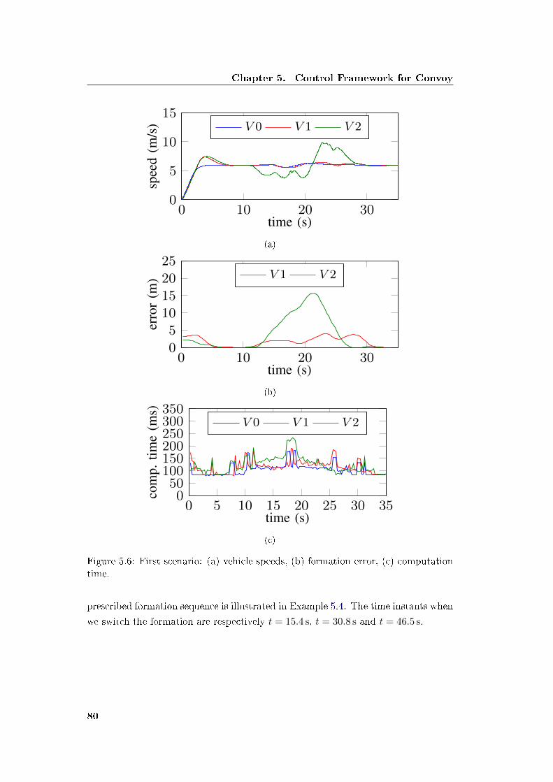
Chapter 5. Control Framework for Convoy
0 10 20 300
5
10
15
time (s)
spee
d(m
/s) V 0 V 1 V 2
(a)
0 10 20 300
5
10
15
20
25
time (s)
erro
r(m
) V 1 V 2
(b)
0 5 10 15 20 25 30 350
50100150200250300350
time (s)
com
p.tim
e(m
s)
V 0 V 1 V 2
(c)
Figure 5.6: First scenario: (a) vehicle speeds, (b) formation error, (c) computationtime.
prescribed formation sequence is illustrated in Example 5.4. The time instants when
we switch the formation are respectively t = 15.4 s, t = 30.8 s and t = 46.5 s.
80

5.6. Concluding remarks
Simulation results
Fig. 5.7 presents the trajectories of the four vehicles during the experiment. This
simulation demonstrates that isomorphic formation changes can be performed smoothly
while avoiding intra-formation collisions. Moreover, the curvy nature of the road is
handled nicely by our framework.
0 50 100 150 200 250 300 35030
20
10
0
10
20
30
x(m)
y(m
)
V0V1V2V3
01
23
01
23 0
1
2
3
01
2
3 0
1
23
0
1
2
3
01
23
0
1
2
3
t = 0
t = 7.7 t = 15.4
t = 23.1 t = 30.8
t = 38.5
t = 46.2
t = 53.9
Figure 5.7: Second scenario: trajectories of four vehicles.
Videos of the two experiments are available on-line1.
5.6 Concluding remarks
We have presented a convoy control framework for multiple vehicles on the road.
The proposed framework is composed of a centralized convoy supervisor and multi-
ple local vehicle controllers. The convoy supervisor centrally manages the geomet-
rical structure of the convoy and while each vehicle locally computes a trajectory
compatible with the formation control, using information exchanged through com-
munication. We have made use of logical rules to handle intra-formation collision
avoidance. Moreover, we have designed a strategy for recon�guration between iso-
morphic formations in a safe and timely manner. High-�delity computer simulations
have demonstrated the e�ectiveness of the approach.
1https://youtu.be/QIGIgCmBr0A
81


Chapter 6
Control Framework for Autonomous
Intersection Management
In previous chapters, we have applied MPC to the motion planning and control of
individual vehicles and convoys of vehicles. In this chapter, we apply MPC to coor-
dinate autonomous vehicles at an intersection without tra�c lights. We propose a
hierarchical control architecture with a centralized intersection controller and mul-
tiple local planners for individual vehicles. The intersection controller decides the
relative crossing orders of vehicles while planners of vehicles compute trajectories
that respect the prescribed orders using MPC based techniques in a receding hori-
zon fashion. The proposed system maintains the system-wide safety property even
if one or more vehicles suddenly brake. Simulations are performed to illustrate the
bene�ts of our approach.
6.1 Introduction
Currently, tra�c lights are installed in many intersections to coordinate con�icting
tra�c �ows. However, there is a rising concern on the e�ciency and safety of these
systems. Taking advantage of current advances in cooperative autonomous driving
technology, studies have been conducted to explore ideas of autonomous intersections
without tra�c lights (Fig. 6.1), as brie�y presented below.
Planning-based approaches [32, 33, 34] �rst compute collision-free trajectories
for all vehicles to cross the intersection without collision; in a second phase, vehicles
are controlled to follow these trajectories. In [32], the optimal speed pro�les for a
two-vehicle intersection are analytically studied assuming simple vehicle behaviors,
while the extension to a multi-vehicle intersection is subject to future work. In [33],
constrained nonlinear optimization techniques are employed to plan trajectories for
all vehicles entering the intersection. The control goal is to minimize the total length
of overlapped trajectories. However, the complexity of the optimization problem
renders the solution hard to obtain.
Though planning-based approaches have good properties since trajectories can
be optimized in advance, a major weakness lies in the di�culty to execute the
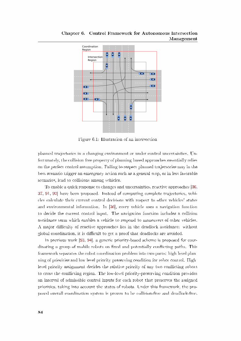
Chapter 6. Control Framework for Autonomous Intersection
Management
CoordinationRegion
IntersectionRegion
Figure 6.1: Illustration of an intersection
planned trajectories in a changing environment or under control uncertainties. Un-
fortunately, the collision-free property of planning-based approaches essentially relies
on the perfect control assumption. Failing to respect planned trajectories may in the
best scenario trigger an emergency action such as a general stop, or in less favorable
scenarios, lead to collisions among vehicles.
To enable a quick response to changes and uncertainties, reactive approaches [36,
37, 91, 92] have been proposed. Instead of computing complete trajectories, vehi-
cles calculate their current control decisions with respect to other vehicles' states
and environmental information. In [36], every vehicle uses a navigation function
to decide the current control input. The navigation function includes a collision
avoidance term which enables a vehicle to respond to maneuvers of other vehicles.
A major di�culty of reactive approaches lies in the deadlock avoidance: without
global coordination, it is di�cult to get a proof that deadlocks are avoided.
In previous work [93, 94], a generic priority-based scheme is proposed for coor-
dinating a group of mobile robots on �xed and potentially con�icting paths. This
framework separates the robot coordination problem into two parts: high-level plan-
ning of priorities and low-level priority-preserving condition for robot control. High-
level priority assignment decides the relative priority of any two con�icting robots
to cross the con�icting region. The low-level priority-preserving condition provides
an interval of admissible control inputs for each robot that preserves the assigned
priorities, taking into account the states of robots. Under this framework, the pro-
posed overall coordination system is proven to be collision-free and deadlock-free.
84

6.2. System model
However, robots in this work are controlled using a simple "bang-bang" control
law, which is fuel ine�cient and maybe uncomfortable, and as such, unsuitable for
autonomous driving.
In this chapter, we combine the priority-based framework with model predictive
control to smoothly coordinate autonomous vehicles at intersection. The proposed
approach inherits the provably-safe and deadlock-free properties of the priority-
based framework, and produces smooth longitudinal trajectories for each individual
vehicle.
The rest of the chapter is articulated as follows. � 6.2 presents the system model
of autonomous intersection. � 6.3 provides an overview of the hierarchical control
architecture. In � 6.4, we present the design of the high-level intersection controller.
In � 6.5, we present the motion planning for individual vehicles; � 6.7 presents the
simulation results. Finally, � 6.8 concludes the chapter.
6.2 System model
Consider a collection of N = {1, ..., N} autonomous vehicles approaching an in-
tersection as shown in Fig. 6.1. The proximity of the intersection is conceptually
divided into two region: the coordination region and the intersection region. We
assume that vehicles are coordinated within the coordination region. The intersec-
tion region is a subset of the coordination region, where only authorized vehicles
can enter. For each vehicle i ∈ N , we make the following assumptions:
1. a predetermined path γi ∈ R is given and is perfectly followed;
2. the velocities of vehicles are always non-negative;
3. perfect communication links can be established with other vehicles and with
a roadside unit called the intersection controller;
4. the current states of vehicles can be acquired (through sensors and/or com-
munication);
Let si ∈ R be the curvilinear coordinate along the path for vehicle i. We ignore
the lateral dynamics of the vehicle and use the double integrator model to describe
the longitudinal dynamics:
si = vi, (6.1a)
vi = ai, (6.1b)
85

Chapter 6. Control Framework for Autonomous Intersection
Management
2 1
(a)
2
1
(b)
2
1
(c)
2 1
(d)
s1
s2
C12
(e)
s1
s2
C12
(f)
s1
s2
C12
(g)
s1
s2
C12
(h)
Figure 6.2: (a) - (d) are illustrations of interactions of paths that we considered inthis paper. (e) - (h) are the corresponding obstacle regions. (a) is the case of twovehicles on the same path and (e) is the obstacle region corresponding to (a), givenas {(s1, s2) : s1 − s2 ≤ d}, where d is the minimum separation of two vehicleson the same path. (b) is the crossing case and (f) is the corresponding obstacleregion given as [L1, H1] × [L2, H2], where [L1, H1] is the interval on the path γ1
where collision with vehicle 2 may occur. (c) is the merging case and (g) is thecorresponding obstacle region given as [L1, H1] × [L2, H2] ∪ {(s1, s2) : |s1 − s2| ≤d, s1 > H1, s2 > H2}. (d) is the diverging case and the corresponding obstacleregion is {(s1, s2) : s1 − s2 ≤ d, s1 ≤ H1}.
with si, vi and ai respectively being the position, speed and acceleration of the
vehicle i. We let the state ξi = [si, vi] and the control input ui = ai. We bound the
speed and the acceleration:
ξi ∈ Ξi := [−∞,+∞]× [0, vi], (6.2a)
ui ∈ Ui := [ui, ui]. (6.2b)
We use ui ∈ Ui to denote an admissible input signal, which is a function of time
ui : t 7→ ui(t) ∈ Ui for t ≥ t0 and we note Ui the space of all admissible control
signals. Let ξi(t,ui, ξi(t0)), si(t,ui, ξi(t0)) and vi(t,ui, ξi(t0)) respectively denote
the state, position and speed of vehicle i at time t, starting from ξi(t0).
For two vehicles i, j ∈ N , we say that i and j are con�icting if γi∩γj 6= ∅ and we
de�ne the obstacle region Cij ⊂ R2 as the set of con�gurations (si, sj) where i and j
collide. We assume that the obstacle region is connected. Note that this de�nition
of the obstacle region is not restricted to the case of crossing paths, but can also be
used for car-following, merging and diverging paths. In the case of non-intersecting
paths, we let Cij = ∅. This formulation can handle general tra�c intersections with
multiple collision points as in Fig. 6.1. Fig. 6.2 illustrates the obstacle regions in
various cases.
86

6.3. Control architecture overview
For every pair of vehicles with non-empty obstacle region, one vehicle necessarily
passes before the other, which naturally leads to the notion of priority. For cases
like Fig. 6.2a or Fig. 6.2d, the initial position of the vehicles implies that vehicle 1
always has priority over vehicle 2. In the other cases (Fig. 6.2b and Fig. 6.2c), a
priority order must be determined. We note i � j if vehicle i has priority over j.
For the sake of simplicity, in the case where Cij = ∅ we accept either i � j or j � i
as valid, but the choice has no in�uence on the behaviors of vehicles.
s2
s1
C12C2�1
Figure 6.3: Completed obstacle region for 2 � 1 of Fig. 6.2f.
Each priority relation corresponds to a homotopy class of trajectories. For ex-
ample, there are two homotopy classes of trajectories in Fig. 6.2f: the class of
trajectories passing above the obstacle region corresponds to 2 � 1 while the class
of trajectories passing under the obstacle region corresponds to 1 � 2. As a result,
choosing an order of priority is equivalent to restricting vehicles to a given homotopy
class of trajectories. We de�ne Ci�j as the completed obstacle region authorizing
all trajectories i � j. Fig. 6.3 illustrates the completed obstacle region C2�1 in the
case of Fig. 6.2b.
6.3 Control architecture overview
Fig. 6.4 gives an overview of the proposed control architecture for autonomous inter-
sections. The system is designed in a hierarchical way with a high-level centralized
intersection controller and low-level, local motion planners for individual vehicles.
The tracking controllers of vehicles are omitted in the �gure for the sake of simplicity.
The intersection controller keeps track of the vehicles that need to coordinate by
incorporating newly arrived vehicles and removing departed vehicles. We assume
that the intersection controller monitors perfectly the states of vehicles through
sensors or V2V communications. The intersection controller assigns priorities to
vehicles in the form of a priority list O. Further details will be provided in � 6.4.
At low-level, each vehicle is controlled locally to cross the intersection and pre-
serve the assigned priorities. We exploit the �exibility of MPC to incorporate
87

Chapter 6. Control Framework for Autonomous Intersection
Management
Intersection Controller
Motion Planner of Vehicle 1
Motion Planner of Vehicle 2
Motion Planner of Vehicle N
Info on Newly Arrived Vehicles
Info on Vehicle Departures
Figure 6.4: Overview of the control architecture for autonomous intersection.
priority-preserving constraints into the formulation of the optimization problem to
ensure the respect of priorities at the planning level. The detailed formulation will
be provided in � 6.5. The states of vehicles are observed by, or communicated to
the intersection controller and other vehicles.
6.4 Intersection controller
The intersection controller coordinates vehicles inside the coordination region using
priorities. Outside the coordination region, vehicles are assumed to drive safely
by other means such as Adaptive Cruising Control (ACC), Cooperative Adaptive
Cruising Control (CACC), etc. A convenient way to encode the priority assignments
is by using a priority graph, de�ned as an oriented graph whose vertices are the
vehicles i ∈ N and where the directed edge i → j exists if and only if i � j. It
is shown in [93] that using a general oriented graph as a priority graph may cause
deadlocks if the graph has cycles. One possible workaround is to �rst design a
priority graph, then use a strongly connected component detection algorithm like
Tarjan's algorithm [95] to detect and remove the potential cycles. In this work, we
use a simpler alternative approach to avoid cycles in the graph: instead of designing
a priority graph from scratch, we choose a permutation of the vehicles of N and use
it as an ordered list of the vehicles, O. Noting σ(i) and σ(j) the respective position
of i and j in O, we then construct a priority graph by adding the edge i→ j to the
graph (and therefore the priority i � j) if and only if σ(i) < σ(j). In other words, Oencodes the order in which the vehicles are allowed to cross the intersection. Note
that for the general case of N vehicles, there are N ! possible graphs that can be
constructed using this algorithm, all of them acyclic.
The intersection controller maintains a simple �nite-state machine for each ve-
88

6.5. Local vehicle controller
hicle in the coordination region. The state machine has two states:
Unassigned: Vehicles are unassigned if they have entered the coordination
region but have not yet been assigned priorities. Unassigned vehicles must remain
outside of the intersection region until they become assigned.
Assigned: Vehicles are assigned if they have been added toO. Assigned vehiclesare allowed to enter the intersection region and must preserve the assigned priorities.
The intersection controller works in discrete time. Vehicles that enter the co-
ordination region notify the intersection controller of their presence. It maintains
the list O (for assigned vehicles) and a waiting list for unassigned vehicles. At each
time step, one or several vehicles can be assigned and added to the list according to
a priority assignment policy. Once vehicles leave the coordination region, they are
removed from the priority list and the corresponding priority relations are revoked.
The priority assignment policy that enables the coordination of vehicles at an
intersection is essentially the �brain� of the intersection controller. The design of an
optimal policy, however, is still an open problem. In [96], the time optimal priority
assignment policy is found using Mixed Integer Linear Programming, assuming that
we have full control of vehicle trajectories. However, the assumption is not valid in
this work as each vehicle computes its own trajectory in a receding horizon fashion
under the priority-preserving constraints.
In practice, we �nd that carefully-designed heuristic policies provide satisfactory
performance. We adopt the Fast First Service (FFS) policy adapted from [93].
For each unassigned vehicle, we simulate its behavior assuming it is added at the
end of the priority list. If, in this case, the vehicle can cross the intersection without
braking while respecting all priorities, then we consider this vehicle as a �fast� vehicle
and e�ectively append it to the priority list. Note that it is possible that there is
no �fast� vehicle at a given time; in this case, the controller simply waits without
adding new vehicles to the priority list. The FFS policy favors the vehicles that
require to stay in the intersection region for a minimum duration, thus increasing
the e�ciency of the system.
6.5 Local vehicle controller
6.5.1 Priority-preserving condition
The priority-preserving condition is deduced in this section. For a pair of vehicles
i, j ∈ N , j being in a state ξ0j at the current time t = 0, we de�ne a set-valued
function:
Bj�i(ξ0j ) :=
{ξi ∈ Ξi
∣∣ ∀t ≥ 0,(si(t,ui, ξi), sj(t,uj , ξ
0j ))/∈ Cj�i
}, (6.3)
89

Chapter 6. Control Framework for Autonomous Intersection
Management
where u is the maximal brake control signal. Therefore, if ξ0i ∈ Bj�i(ξ0
j ) then vehicle
i can come to a stop without entering the completed obstacle region even if vehicle
j brakes at its maximum for all t ≥ 0. We introduce the de�nition of brake-safe
state:
De�nition 6.1 (Brake-safe state). Consider a vehicle i, it is in brake-safe state ξ0i
if and only if, for all j � i, ξ0i ∈ Bj�i(ξ0
j ).
If i is in a brake-safe state (or, more simply, i is brake-safe), it can always stop
before violating any of its assigned priorities even if another vehicle brakes at its
maximum. However, since vehicles are controlled digitally, their reactions to a brake
event will at most have a delay of τ , which is the update interval of the control. We
further introduce the de�nition of brake-safe control as:
De�nition 6.2 (Brake-safe control). Assuming that i starts in an initial brake-safe
state ξ0i , a constant control input ui de�ned over [0, τ) such that ∀t ∈ [0, τ),ui(t) =
ui, is said to be a brake-safe control if
∀j � i, ξi(τ,ui, ξ0i ) ∈ Bj�i
(ξj(τ,uj , ξ
0j )). (6.4)
This condition states that the input ui for [0, τ) is a brake-safe control if the state
of vehicle i at τ under control ui is still brake-safe with regard to any vehicle j � iapplying a maximal brake command during this period. To simplify the notation,
we write (6.4) compactly as
ui ∈⋂j�iUj�i(ξ0
i , ξ0j , τ), (6.5)
where Uj�i is a set-valued function returning the set of all constant control inputs
for [0, τ) that are brake-safe with regard to vehicle j and⋂j�i Uj�i(ξ0
i , ξ0j , τ) is the
intersection of all such sets for all j � i.If vehicle i is brake-safe, the set (6.5) is a non-empty open interval that contains
necessarily ui. The length of this interval corresponds to the leeway vehicle i has in
choosing a control.
For assigned vehicles, the brake-safe condition (6.5) must be respected during
the entire crossing so that they always respect the assigned priorities.
For unassigned vehicles, default priority relation exists. Notably, an unassigned
vehicle should remain brake-safe with regard to the front vehicle if it exists. We
denote this condition as
ui ∈ Uprev�i(ξ0i , ξ
0prev, τ), (6.6)
90

6.5. Local vehicle controller
where ξprev is the state of the preceding vehicle. At the same time, it must maintain
brake-safety with regard to the entry of the intersection region: it cannot enter the
intersection region unless it is assigned. Let Ei be the curvilinear coordinate of the
entry of the intersection zone for vehicle i. Maintaining brake-safety with regard to
Ei can be considered as maintaining brake-safe with regard to a virtual vehicle ν
stationed at Eiui ∈ Uν�i(ξ0
i , ξ0ν , τ), (6.7)
where ξ0ν = [Ei, 0] is the state of the virtual vehicle.
Remark that the de�nition of brake-safe control seems to assume that the other
vehicles brake at their maximum. However, since the dynamics of the system is
monotone [97], condition (6.4) in fact ensures that future states of vehicle i will still
be brake-safe regardless of the actual control applied by the other vehicles.
6.5.2 MPC formulation
Let T denote the length of prediction horizon and τ be the update interval of the
control. We have T = Kτ with K being the total discretized steps.
We let uki , vki , s
ki and ξki respectively represent the control, speed, position and
state of vehicle i at time kτ . The discrete-time state equation can then be given by
ξk+1i = Adξki +Bduki (6.8)
where Ad = ( 1 τ0 1 ) and Bd = (
12τ2
τ).
The longitudinal trajectory of a vehicle i can be generated using the following
MPC formulation:
minuiJi(ξ, ui) = min
ui
K∑k=0
Li(ξki , uki ) (6.9)
subject to ∀k ∈ [0, ...,K],
ξi(0) = ξi, (6.10a)
ξki ∈ Ξi, uki ∈ Ui, (6.10b)
ξk+1i = Adxki +Bduki , (6.10c)
uki ∈⋂j�iUj�i(ξki , ξkj , τ), if the vehicle is assigned, (6.10d)
uki ∈ Uprev�i(ξki , ξkprev, τ)⋂Uν�i(ξki , ξkν , τ), if the vehicle is unassigned, (6.10e)
91

Chapter 6. Control Framework for Autonomous Intersection
Management
where Ji denotes the cost function to be minimized by selecting a proper sequence
of control input uki , k = 0, ...,K. Li denotes is running cost during the interval τ .
We may select a quadratic running cost as
Lki = qi,1(vdi − vki )2 + qi,2(uki )2 (6.11)
where the �rst term is the e�ciency cost (gap between the current speed and the
target speed) and the second term penalizes the control signal. We may consider
other metrics to evaluate the cost rather than the one proposed here. (6.10a)
and (6.10b) respectively de�ne the initial condition and the boundary constraints.
Equation (6.10c) is the state transition constraint that describes the time-dependent
evolution of the system. We enforce the priority-preserving constraint at each time
step k = 0, ...,K in (6.10d) and (6.10e).
Remark that it is not necessary to enforce the priority-preserving constraint at
every time step in the prediction horizon, because only the constraint at the �rst
time step is required to guarantee the output to be priority-preserving. However,
we opt to enforce constraints at the future time steps since it allows the vehicle to
react earlier to possible priority violations in the future. Such enforcement requires
the knowledge of ξkj for k ∈ [0, ...,K]. We have assumed that each vehicle knows the
current states of its prior vehicles. The future states of prior vehicles can be esti-
mated by using prediction models, or simpler, by exchanging intentions (previously
computed trajectories) using V2V communication.
6.6 Theoretic results for the proposed design
The proposed control architecture has the following properties:
Theorem 6.1 (Recursive feasibility). The optimization problem (6.9) is recursively
feasible if the current vehicle state is brake-safe with regard to prior vehicles.
The proof is intuitive. A vehicle in brake-safe state ensures that there exists a
feasible control input at time τ regardless of other vehicles' maneuvers. Thus the
MPC problem will also be feasible at time τ .
Theorem 6.2 (Robust safety). Even if one or more vehicles fail to respect the
computed trajectories and perform emergency brakes, the system is still safe.
The reason is that the maximal brake command ui is a brake-safe control. Thus
the system remains safe. Detailed proof is available in [98].
Theorem 6.3 (Deadlock-freeness). All vehicles eventually quit the intersection.
92

6.7. Simulation
In [98], it is shown that if there is no cyclic priority relations, then the system
is deadlock-free. Since we use a cycle-free priority list O to encode the priority
relations, then no deadlock will occur.
6.7 Simulation
Scenario description
0 25 50 75 1000
25
50
75
100
x(m)
y(m)
Vehicle 1
Vehicle 2
Vehicle 3
Figure 6.5: Intersection layout for simulation
We illustrate the approach through simulation with a simple intersection illus-
trated in Fig. 6.5. We consider a system of three vehicles labeled by numbers 1, 2
and 3. Vehicle 1, 2 and 3 drive respectively with the direction of West-East, South-
North and North-South. We determine the priorities as 1 � 2 and 1 � 3. The
priority relation between vehicle 2 and vehicle 3 are not relevant since their paths
do not intersect. Vehicles start at position s1 = s2 = s3 = 0. Their dynamics are
supposed to be identical such that Vi = [0, 8] m/s and Ui = [−3, 2] m/s2. The initial
velocities of three vehicles are set to 8 m/s. The parameters of the cost function
are set to vdi = 8 m/s, qi,1 = 1 and qi,2 = 3.
Simulation results
In the simulation, the duration of a time step is set to τ = 0.2 s and the prediction
horizon is set to T = 3 s.
We run simulations with two di�erent scenarios: in the �rst scenario vehicle
1 crosses the intersection at its desired speed; in the second scenario, vehicle 1
performs an emergency braking with ui = −3 m/s2 between t = 2.6 s and t = 5.2 s.
93

Chapter 6. Control Framework for Autonomous Intersection
Management
Fig. 6.6 illustrates the system trajectories of two scenarios in the position space.
We observe that in both scenarios the system trajectories do not intersect with the
obstacle region. Fig. 6.7 and Fig. 6.8 are respectively the speed and acceleration
pro�les for the two scenarios. We observe that the proposed MPC scheme generates
smooth longitudinal trajectories for vehicles. Safety is guaranteed in both scenarios.
In the second scenario, vehicle 2 and vehicle 3 adapt their speeds when vehicle 1
performs an emergency brake to avoid collisions.
A video is available1 to illustrate the capacity of the proposed scheme in handling
a continuous �ow of vehicles using the proposed priority assignment method.
1https://youtu.be/3iHGNgW61-s
94

6.7. Simulation
0 40 80 0 40 800
20
40
60
80
s1(m) s2(m)
s 3(m
)
(a)
0 40 80 0 40 800
20
40
60
80
s1(m) s2(m)
s 3(m
)
(b)
Figure 6.6: Position space of three vehicles in the simulation. Sub�gure (a) shows thesystem trajectory as well as the obstacle region in the normal driving case, sub�gure(b) shows the system trajectory when the vehicle 1 performs an emergency brake.The interval of emergency brake is colored in red.
95

Chapter 6. Control Framework for Autonomous Intersection
Management
0 4 8 120
5
10
t(s)
v(m/s) 1 2 3
(a)
0 4 8 12−3
0
3
6
t(s)
a(m/s
2) 1 2 3
(b)
Figure 6.7: Speed and acceleration pro�les for the �rst scenario. Vehicle 2 andvehicle 3 decelerate to yield passage to vehicle 1. The speed pro�les of all vehiclesare smooth.
0 4 8 12 160
5
10
t(s)
v(m/s) 1 2 3
(a)
0 4 8 12 16−3
0
3
6
t(s)
a(m/s
2) 1 2 3
(b)
Figure 6.8: Speed and acceleration pro�les for the second scenario. Vehicle 1 is forcedto perform an emergency brake. Vehicle 2 and vehicle 3 adapt correspondingly theirspeed to avoid collision.
96

6.8. Concluding remarks
6.8 Concluding remarks
We have presented a hierarchical control architecture for autonomous intersections.
The architecture is comprised of a centralized intersection controller for priority as-
signment and local motion planners for individual vehicles that are con�gured to re-
spect the priorities. The integration of priority-based framework with MPC ensures
individual vehicles to have smooth trajectories and the system to be deadlock-free
and robustly safe.
97


Chapter 7
Conclusions and perspectives
In the last decade, autonomous driving has been attracting more and more atten-
tions from both industrial actors and academic institutes thanks to its capability in
enhancing tra�c e�ciency and reducing accidents. In this thesis, we have consid-
ered two major challenges in autonomous driving: how to guide vehicles to proceed
in an on-road environment populated with obstacles and governed by tra�c rules,
and how to make autonomous vehicles maneuver cooperatively ?
We have partially dealt with these challenges in our thesis. We started with
the �rst challenge. We presented a hierarchical control architecture that employs
an MPC based motion planner for trajectory generation and another MPC based
tracking controller for trajectory tracking. We demonstrated the capability of this
design in di�erent on-road driving scenario. However, further analysis demonstrated
that the motion planner in this design cannot handle an important category of con-
straints: logical constraints. To cope with this issue, we presented a hybrid MPC
based motion planner that is able to handle both di�erentiable constraints and log-
ical constraints by formulating the motion planning problem as a Mixed Integer
Quadratic Programming problem. We applied the planner to various scenarios (in-
tersection crossing, obstacle avoidance, overtaking, lane change, etc.) to illustrate
the advantages of this planner.
We responded to the second challenge with two control designs for cooperative
autonomous driving: a control architecture for convoy control of autonomous vehi-
cles and a control architecture for autonomous intersection management. For the
formation control problem, we presented a hierarchical framework with a convoy su-
pervisor to manage and recon�gure the formation and local MPC based controllers
to track the formation-keeping reference trajectories while satisfying various con-
straints. We made use of logical rules to handle intra-formation collision avoidance
and proposed a strategy for recon�guration between isomorphic formations in a
safe and timely manner. For the autonomous intersection management problem, we
adopted the priority-based coordination framework and separated the autonomous
intersection management problem into a priority assignment problem and a vehicle
control problem. A centralized intersection controller is designed to assign priori-
ties to incoming vehicles following a priority assignment policy. Local MPC based

Chapter 7. Conclusions and perspectives
vehicle planners generate optimal trajectories while respect the assigned priorities.
The proposed design ensures the system to be safe to unexpected events (emergency
braking) and allow vehicles to cross the intersection safely.
Perspectives
Hybrid MPC based planner
The hybrid MPC based planner uses a linear point mass model in the formulation of
model predictive control problem. This model is suitable if the longitudinal motion
dominates the lateral one, for example when driving on highways or on urban arterial
roads. However, for some applications, a nonlinear vehicle model might be more
desirable. Future work will investigate the applicability of combining the feedback
linearizion with the MIQP formulation. Another important assumption in this paper
is that the vehicle is driving on road segments with small curvature. For large road
curvatures, the current model can be imprecise. This issue should be investigated
in the future.
We have not considered in detail the problem of estimating the trajectories of
surrounding obstacles. Constant velocity assumption is used in this work. However,
uncertainties in estimation can raise from sensor noises and hard-to-estimate inten-
tions of other tra�c participants. It will be useful to investigate the integration of
probabilistic trajectory predictions of obstacles with the motion planner. Finally,
the design requires more validation in simulations and �eld experiments.
Control framework for convoy
More work can be done to enhance the control design for vehicle convoys. The
collision avoidance rules can be further analyzed and enhanced. It will also be useful
to consider high-level decision-making process for recon�gurations of convoys and
to investigate algorithms that can compute automatically the formation sequences
from an initial formation to a desired one. Finally, we should evaluate this approach
using real vehicles and under realistic perception and communication conditions.
Control framework for autonomous intersection management
We adopted a simple Fast First Service policy for priority assignment, more sophisti-
cated policies that take into account parameters like queue lengths or vehicles idling
time can be developed. Furthermore, the proposed framework can also be extended
to more complex intersection geometries like roundabouts, or multiple intersections.
Finally, �eld experiments of the proposed architecture will also be bene�cial for
100

understanding the impacts from noisy perception, unreliable communication and
nonlinear vehicle dynamics on the autonomous intersection management.
101


Bibliography
[1] Kurt M Dresner and Peter Stone. A Multiagent Approach to Autonomous In-
tersection Management. J. Artif. Intell. Res.(JAIR), 31:591�656, 2008. (Cited
on pages v and 6.)
[2] Philipp Bender, Omer Sahin Tas, Julius Ziegler, and Christoph Stiller. The
combinatorial aspect of motion planning: Maneuver variants in structured en-
vironments. In Intelligent Vehicles Symposium (IV), 2015 IEEE, pages 1386�
1392. IEEE, 2015. (Cited on pages vi, 3, 27, 42, 43 and 58.)
[3] Chris Urmson, Joshua Anhalt, Drew Bagnell, Christopher Baker, Robert Bit-
tner, MN Clark, John Dolan, Dave Duggins, Tugrul Galatali, Chris Geyer,
et al. Autonomous driving in urban environments: Boss and the urban chal-
lenge. Journal of Field Robotics, 25(8):425�466, 2008. (Cited on page 1.)
[4] Julius Ziegler, Philipp Bender, Markus Schreiber, Henning Lategahn, Tobias
Strauss, Christoph Stiller, Thao Dang, Uwe Franke, Nils Appenrodt, and
Christoph G. Keller. Making bertha drive-an autonomous journey on a his-
toric route. IEEE Intelligent Transportation Systems Magazine, 6:8�20, 2014.
(Cited on page 1.)
[5] BMW. Bmw group, intel and mobileye team up to
bring fully autonomous driving to streets by 2021, 2016.
https://www.press.bmwgroup.com/global/article/detail/T0261586EN/bmw-
group-intel-and-mobileye-team-up-to-bring-fully-autonomous-driving-to-
streets-by-2021?language=en, accessed 13/08/2016. (Cited on page 1.)
[6] Google. Google self-driving car project, 2016.
https://www.google.com/selfdrivingcar/, accessed 18/08/2016. (Cited on
page 1.)
[7] PSA. Roadmap to the autonomous car, 2016. http://www.psa-peugeot-
citroen.com/en/featured-content/autonomous-car, accessed 18/08/2016.
(Cited on page 1.)
[8] Arnaud De La Fortelle, Xiangjun Qian, Sébastien Diemer, Jean Grégoire, Fa-
bien Moutarde, Silvere Bonnabel, Ali Marjovi, Alcherio Martinoli, Ignacio
Llatser, Andreas Festag, et al. Network of automated vehicles: the autonet2030
vision. In 21st World Congress on Intelligent Transport Systems, 2014. (Cited
on pages 1, 4 and 5.)

Bibliography
[9] E. Galceran, R. M. Eustice, and E. Olson. Toward integrated motion planning
and control using potential �elds and torque-based steering actuation for au-
tonomous driving. In 2015 IEEE Intelligent Vehicles Symposium (IV), pages
304�309, June 2015. (Cited on pages 2 and 23.)
[10] Boliang Yi, Stefan Gottschling, Jens Ferdinand, and Frank Bonarens. Real
time integrated vehicle dynamics control and trajectory planning with mpc for
critical maneuvers. In IEEE Intelligent Vehicles Symposium, 2016. (Cited on
pages 2, 23 and 24.)
[11] B. Paden, M. Cap, S. Yong, D. Yershov, and E. Frazzoli. A survey of motion
planning and control. IEEE Transactions on Intelligent Vehicles, PP(99):1�1,
2016. (Cited on page 2.)
[12] D. Gonzalez, J. Perez, V. Milanes, and F. Nashashibi. A review of motion
planning techniques for automated vehicles. IEEE Transactions on Intelligent
Transportation Systems, 17(4):1135�1145, April 2016. (Cited on page 2.)
[13] M. McNaughton, C. Urmson, J. M. Dolan, and J. W. Lee. Motion planning
for autonomous driving with a conformal spatiotemporal lattice. In Robotics
and Automation (ICRA), 2011 IEEE International Conference on, pages 4889�
4895, May 2011. (Cited on pages 2, 23 and 24.)
[14] Yoshiaki Kuwata, Justin Teo, Gaston Fiore, Sertac Karaman, Emilio Frazzoli,
and Jonathan P. How. Real-time motion planning with applications to au-
tonomous urban driving. IEEE Transactions on Control Systems Technology,
17(5):1105�1118, 2009. (Cited on pages 2, 23 and 24.)
[15] Liang Ma, Jianru Xue, Kuniaki Kawabata, Jihua Zhu, Chao Ma, and Nanning
Zheng. E�cient Sampling-Based Motion Planning for On-Road Autonomous
Driving. IEEE Transactions on Intelligent Transportation Systems, pages 1�16,
2015. (Cited on pages 2, 23 and 24.)
[16] David González, JM Perez, Ray Lattarulo, Vicente Milanés, and Fawzi
Nashashibi. Continuous curvature planning with obstacle avoidance capabil-
ities in urban scenarios. In Intelligent Transportation Systems (ITSC), 2014
IEEE 17th International Conference on, pages 1430�1435. IEEE, 2014. (Cited
on pages 2 and 23.)
[17] Tianyu Gu and John M. Dolan. Toward human-like motion planning in urban
environments. 2014 IEEE Intelligent Vehicles Symposium Proceedings, pages
350�355, June 2014. (Cited on pages 2, 23 and 24.)
104

Bibliography
[18] Julius Ziegler, Philipp Bender, Thao Dang, and Christoph Stiller. Trajectory
planning for Bertha - A local, continuous method. IEEE Intelligent Vehicles
Symposium, Proceedings, (Iv):450�457, 2014. (Cited on pages 3, 17 and 24.)
[19] Yiqi Gao. Model Predictive Control for Autonomous and Semiautonomous Vehi-
cles. PhD thesis, UNIVERSITY OF CALIFORNIA, BERKELEY, 2014. (Cited
on pages 3, 4, 12, 14, 15, 17, 21, 23, 24, 42, 43 and 46.)
[20] Julia Nilsson, Paolo Falcone, Mohammad Ali, and Jonas Sjöberg. Receding
horizon maneuver generation for automated highway driving. Control Engi-
neering Practice, 41:124�133, 2015. (Cited on pages 3, 46, 58 and 59.)
[21] T. Weiskircher and B. Ayalew. Predictive adas: A predictive trajectory guid-
ance scheme for advanced driver assistance in public tra�c. In Control Confer-
ence (ECC), 2015 European, pages 3402�3407, July 2015. (Cited on pages 3,
21 and 42.)
[22] S E Shladover, C A Desoer, J K Hedrick, M Tomizuka, J Walrand, W.-B. Zhang,
D H McMahon, H Peng, S Sheikholeslam, and N McKeown. Automated vehi-
cle control developments in the PATH program. Vehicular Technology, IEEE
Transactions on, 40(1):114�130, February 1991. (Cited on pages 4 and 69.)
[23] L. Bouraoui, S. Petti, A. Laouiti, T. Fraichard, and M. Parent. Cybercar
cooperation for safe intersections. In 2006 IEEE Intelligent Transportation
Systems Conference, pages 456�461, Sept 2006. (Cited on pages 4 and 69.)
[24] L. Hobert, A. Festag, I. Llatser, L. Altomare, F. Visintainer, and A. Kovacs.
Enhancements of v2x communication in support of cooperative autonomous
driving. IEEE Communications Magazine, 53(12):64�70, Dec 2015. (Cited on
page 4.)
[25] I. Llatser, S. Kuhlmorgen, A. Festag, and G. Fettweis. Greedy algorithms for
information dissemination within groups of autonomous vehicles. In 2015 IEEE
Intelligent Vehicles Symposium (IV), pages 1322�1327, June 2015. (Cited on
page 4.)
[26] I. Llatser, A. Festag, and G. Fettweis. Vehicular communication performance
in convoys of automated vehicles. In 2016 IEEE International Conference on
Communications (ICC), pages 1�6, May 2016. (Cited on page 4.)
[27] Marcus Obst, Laurens Hobert, and Pierre Reisdorf. Multi-sensor data fusion
for checking plausibility of v2v communications by vision-based multiple-object
105

Bibliography
tracking. In 2014 IEEE Vehicular Networking Conference (VNC), pages 143�
150. IEEE, 2014. (Cited on page 4.)
[28] B J Harker. PROMOTE-CHAUFFEUR II & 5.8 GHz vehicle to vehicle com-
munications system. In Advanced Driver Assistance Systems, 2001. ADAS.
International Conference on (IEE Conf. Publ. No. 483), pages 81�85, 2001.
(Cited on pages 4 and 69.)
[29] Eric Chan, Peter Gilhead, Pavel Jelínek, Petr Krej£í, Tom Robinson, Science
Park, Milton Road, Cambridge Cb, and United Kingdom. Cooperative control
of SARTRE automated platoon vehicles. pages 1�9. (Cited on pages 4 and 69.)
[30] A Marjovi, M Vasic, J Lemaitre, and A Martinoli. Distributed graph-based
convoy control for networked intelligent vehicles. In Intelligent Vehicles Sym-
posium (IV), 2015 IEEE, pages 138�143, June 2015. (Cited on pages 4, 6, 69
and 70.)
[31] Shin Kato, Sadayuki Tsugawa, Kiyohito Tokuda, Takeshi Matsui, and Haruki
Fujii. Vehicle Control Algorithms for Cooperative Driving with Automated
Vehicles and Intervehicle Communications. IEEE Transactions on Intelligent
Transportation Systems, 3(3):155�160, 2002. (Cited on pages 6 and 70.)
[32] A.C. Charalampidis and D. Gillet. Speed pro�le optimization for vehicles cross-
ing an intersection under a safety constraint. In European Control Conference
(ECC), 2014, pages 2894�2901, June 2014. (Cited on pages 5 and 83.)
[33] Joyoung Lee and Byungkyu Park. Development and Evaluation of a Coopera-
tive Vehicle Intersection Control Algorithm Under the Connected Vehicles Envi-
ronment. Intelligent Transportation Systems, IEEE Transactions on, 13(1):81�
90, 2012. (Cited on pages 5, 6 and 83.)
[34] A. de La Fortelle. Analysis of reservation algorithms for cooperative planning
at intersections. In Intelligent Transportation Systems (ITSC), 2010 13th In-
ternational IEEE Conference on, pages 445�449, Sept 2010. (Cited on pages 5
and 83.)
[35] I H Zohdy, R K Kamalanathsharma, and H Rakha. Intersection manage-
ment for autonomous vehicles using iCACC. In Intelligent Transportation Sys-
tems (ITSC), 2012 15th International IEEE Conference on, pages 1109�1114,
September 2012. (Cited on page 6.)
[36] Laleh Makarem, Minh Hai Pham, André-Gilles Dumont, and Denis Gillet.
Micro-simulation Modeling of Coordination of Automated Guided Vehicles at
106

Bibliography
Intersection. In Transportation research board 91st annual meeting, 2012. (Cited
on pages 6 and 84.)
[37] L. Makarem and D. Gillet. Model predictive coordination of autonomous vehi-
cles crossing intersections. In Intelligent Transportation Systems - (ITSC), 2013
16th International IEEE Conference on, pages 1799�1804, Oct 2013. (Cited on
pages 6 and 84.)
[38] A Galip Ulsoy, Huei Peng, and Melih Çakmakci. Automotive control systems.
Cambridge University Press, 2012. (Cited on page 12.)
[39] Rajesh Rajamani. Vehicle dynamics and control. Springer Science & Business
Media, 2011. (Cited on pages 12, 15 and 17.)
[40] Jason Kong, Mark Pfei�er, Georg Schildbach, and Francesco Borrelli. Kine-
matic and Dynamic Vehicle Models for Autonomous Driving Control Design.
pages 2�7. (Cited on page 15.)
[41] T. Weiskircher and B. Ayalew. Predictive adas: A predictive trajectory guid-
ance scheme for advanced driver assistance in public tra�c. In Control Confer-
ence (ECC), 2015 European, pages 3402�3407, July 2015. (Cited on page 17.)
[42] Jacques Richalet, A Rault, JL Testud, and J Papon. Model predictive heuristic
control: Applications to industrial processes. Automatica, 14(5):413�428, 1978.
(Cited on page 17.)
[43] B Houska, H J Ferreau, and M Diehl. ACADO Toolkit � An Open Source
Framework for Automatic Control and Dynamic Optimization. Optimal Control
Applications and Methods, 32(3):298�312, 2011. (Cited on pages 17, 32, 51
and 78.)
[44] Inc. Gurobi Optimization. Gurobi optimizer reference manual, 2015. (Cited on
pages 17, 21 and 51.)
[45] Mordecai Avriel. Nonlinear programming: analysis and methods. Courier Cor-
poration, 2003. (Cited on page 19.)
[46] IBM. User's manual for cplex. International Business Machines Corporation,
46(53):157, 2009. (Cited on page 21.)
[47] Sasa V Rakovic and Mirko Fiacchini. Invariant approximations of the maximal
invariant set or "encircling the square". IFAC Proceedings Volumes, 41(2):6377�
6382, 2008. (Cited on page 21.)
107

Bibliography
[48] David Q Mayne, James B Rawlings, Christopher V Rao, and Pierre OM
Scokaert. Constrained model predictive control: Stability and optimality. Au-
tomatica, 36(6):789�814, 2000. (Cited on page 21.)
[49] Lalo Magni and Rodolphe Sepulchre. Stability margins of nonlinear receding-
horizon control via inverse optimality. Systems & Control Letters, 32(4):241�
245, 1997. (Cited on page 22.)
[50] POM Scokaert and DQ Mayne. Min-max feedback model predictive con-
trol for constrained linear systems. IEEE Transactions on Automatic control,
43(8):1136�1142, 1998. (Cited on page 22.)
[51] Arthur Richards and Jonathan How. Robust stable model predictive control
with constraint tightening. In 2006 American Control Conference, pages 6�pp.
IEEE, 2006. (Cited on page 22.)
[52] Wilbur Langson, Ioannis Chryssochoos, SV Rakovi¢, and David Q Mayne. Ro-
bust model predictive control using tubes. Automatica, 40(1):125�133, 2004.
(Cited on page 22.)
[53] Sergio Lucia, Tiago Finkler, and Sebastian Engell. Multi-stage nonlinear model
predictive control applied to a semi-batch polymerization reactor under uncer-
tainty. Journal of Process Control, 23(9):1306�1319, 2013. (Cited on page 22.)
[54] Yiqi Gao, Andrew Gray, H Eric Tseng, and Francesco Borrelli. A tube-based ro-
bust nonlinear predictive control approach to semiautonomous ground vehicles.
Vehicle System Dynamics, 52(6):802�823, 2014. (Cited on page 22.)
[55] Andrew Jacob Gray. An integrated framework for planning and control of
semi-autonomous vehicles. 2013. (Cited on page 23.)
[56] Boris Lau, Christoph Sprunk, and Wolfram Burgard. Kinodynamic motion
planning for mobile robots using splines. 2009 IEEE/RSJ International Con-
ference on Intelligent Robots and Systems, pages 2427�2433, 2009. (Cited on
pages 23 and 24.)
[57] K Kant and S W Zucker. Toward E�cient Trajectory Planning: The Path-
Velocity Decomposition. International Journal of Robotics Research, 5(3):72�
89, 1986. (Cited on page 24.)
[58] Bryan Nagy and Alonzo Kelly. TRAJECTORY GENERATION FOR CAR-
LIKE ROBOTS USING CUBIC CURVATURE POLYNOMIALS Bryan Nagy
and Alonzo Kelly. 2001. (Cited on page 24.)
108

Bibliography
[59] Cheng Chen, Yuqing He, Chunguang Bu, Jianda Han, and Xuebo Zhang. Quar-
tic bezier curve based trajectory generation for autonomous vehicles with curva-
ture and velocity constraints. In Robotics and Automation (ICRA), 2014 IEEE
International Conference on, pages 6108�6113, May 2014. (Cited on page 24.)
[60] Chebly Alia, Tagne Gilles, Talj Reine, and Charara Ali. Local trajectory plan-
ning and tracking of autonomous vehicles, using clothoid tentacles method. In
Intelligent Vehicles Symposium (IV), 2015 IEEE, pages 674�679. IEEE, 2015.
(Cited on page 24.)
[61] Jorge Villagra, Vicente Milanés, Joshué Pérez Rastelli, Jorge Godoy, and En-
rique Onieva. Path and speed planning for smooth autonomous navigation. In
IV 2012-IEEE Intelligent Vehicles Symposium, 2012. (Cited on page 24.)
[62] Wenda Xu, Jia Pan, Junqing Wei, and John M Dolan. Motion planning un-
der uncertainty for on-road autonomous driving. In Robotics and Automa-
tion (ICRA), 2014 IEEE International Conference on, pages 2507�2512. IEEE,
2014. (Cited on page 24.)
[63] Xiaohui Li, Zhenping Sun, Zhen He, Qi Zhu, and Daxue Liu. A practical
trajectory planning framework for autonomous ground vehicles driving in urban
environments. In Intelligent Vehicles Symposium (IV), 2015 IEEE, pages 1160�
1166. IEEE, 2015. (Cited on page 24.)
[64] Julia Nilsson, Yiqi Gao, Ashwin Carvalho, and Francesco Borrelli. Manoeuvre
generation and control for automated highway driving. In The 19th world
congress of the international federation of automatic control (IFAC), 2014.
(Cited on page 24.)
[65] Juergen Ackermann, Jurgen Guldner, Wolfgang Sienel, Reinhold Steinhauser,
and Vadim I Utkin. Linear and nonlinear controller design for robust automatic
steering. IEEE Transactions on Control Systems Technology, 3(1):132�143,
1995. (Cited on page 24.)
[66] S Antonov, A Fehn, and A Kugi. A new �atness-based control of lateral vehicle
dynamics. Vehicle System Dynamics, 46(9):789�801, 2008. (Cited on page 24.)
[67] L. Menhour, B. d'Andrea Novela-Novel, M. Fliess, D. Gruyer, and H. Mounier.
A new model-free design for vehicle control and its validation through an ad-
vanced simulation platform. In Control Conference (ECC), 2015 European,
pages 2114�2119, July 2015. (Cited on page 24.)
109

Bibliography
[68] O Michel. Webots: Professional Mobile Robot Simulation. International
Journal of Advanced Robotic Systems, 1(BIOROB-ARTICLE-2004-001):39�42,
2004. (Cited on pages 32 and 78.)
[69] Ömer �ahin Ta³. Integrating Combinatorial Reasoning and Continuous Meth-
ods for Optimal Motion Planning of Autonomous Vehicles. Master's the-
sis, Karlsruhe Institute of Technology, Germany, September 2014. (Cited on
page 42.)
[70] J. Park, S. Karumanchi, and K. Iagnemma. Homotopy-based divide-and-
conquer strategy for optimal trajectory planning via mixed-integer program-
ming. IEEE Transactions on Robotics, 31(5):1101�1115, Oct 2015. (Cited on
pages 42 and 43.)
[71] Dimitri P Bertsekas. Nonlinear programming. Athena scienti�c Belmont, 1999.
(Cited on page 42.)
[72] Qian Wang, Thomas Weiskircher, and Beshah Ayalew. Hierarchical hybrid pre-
dictive control of an autonomous road vehicle. In ASME 2015 Dynamic Systems
and Control Conference, pages V003T50A006�V003T50A006. American Soci-
ety of Mechanical Engineers, 2015. (Cited on page 43.)
[73] Jon Lee and Sven Ley�er. Mixed integer nonlinear programming, volume 154.
Springer Science & Business Media, 2011. (Cited on page 43.)
[74] Alberto Bemporad and MPC Explicit. Model predictive control of hybrid sys-
tems. University of Siena, Italy, Technical Report, 2005. (Cited on page 43.)
[75] Tom Schouwenaars, Éric Féron, and Jonathan How. Safe receding horizon
path planning for autonomous vehicles. In Proceedings of the Annual Allerton
Conference on Communication, Control and Computing, volume 40, pages 295�
304. The University; 1998, 2002. (Cited on page 43.)
[76] John Bellingham, Arthur Richards, and Jonathan P How. Receding horizon
control of autonomous aerial vehicles. In American Control Conference, 2002.
Proceedings of the 2002, volume 5, pages 3741�3746. IEEE, 2002. (Cited on
page 43.)
[77] Francesco Borrelli, Paolo Falcone, Tamas Keviczky, Jahan Asgari, and Davor
Hrovat. Mpc-based approach to active steering for autonomous vehicle systems.
International Journal of Vehicle Autonomous Systems, 3(2-4):265�291, 2005.
(Cited on page 43.)
110

Bibliography
[78] Johan Nilsson and Jonas Sjoberg. Strategic decision making for automated
driving on two-lane, one way roads using model predictive control. In Intelligent
Vehicles Symposium (IV), 2013 IEEE, pages 1253�1258. IEEE, 2013. (Cited
on pages 43 and 62.)
[79] Yaoqiong Du, Yizhou Wang, and Ching-Yao Chan. Autonomous lane-change
controller via mixed logical dynamical. In Intelligent Transportation Systems
(ITSC), 2014 IEEE 17th International Conference on, pages 1154�1159. IEEE,
2014. (Cited on pages 43 and 62.)
[80] Michel Fliess, Jean Lévine, Philippe Martin, and Pierre Rouchon. Flatness and
defect of non-linear systems: introductory theory and examples. International
journal of control, 61(6):1327�1361, 1995. (Cited on page 46.)
[81] Wayne L Winston, Munirpallam Venkataramanan, and Je�rey B Goldberg.
Introduction to mathematical programming, volume 1. Thomson/Brooks/Cole,
2003. (Cited on pages 47 and 48.)
[82] G. Schildbach, M. Soppert, and F. Borrelli. A collision avoidance system at
intersections using robust model predictive control. In 2016 IEEE Intelligent
Vehicles Symposium (IV), pages 233�238, June 2016. (Cited on page 52.)
[83] Nikolce Murgovski, Jonas Sj, et al. Predictive cruise control with autonomous
overtaking. In 2015 54th IEEE Conference on Decision and Control (CDC),
pages 644�649. IEEE, 2015. (Cited on pages 58 and 59.)
[84] Masahiro Ono, Greg Droge, Havard Grip, Olivier Toupet, Chris Scrapper, and
Amir Rahmani. Road-Following Formation Control of Autonomous Ground
Vehicles. (Cdc):4714�4721, 2015. (Cited on pages 69 and 79.)
[85] J Shao, G Xie, and L Wang. Leader-following formation control of multiple
mobile vehicles. Control Theory Applications, IET, 1(2):545�552, March 2007.
(Cited on page 69.)
[86] Luca Consolini, Fabio Morbidi, Domenico Prattichizzo, and Mario Tosques.
Leader�follower formation control of nonholonomic mobile robots with input
constraints. Automatica, 44(5):1343�1349, 2008. (Cited on page 69.)
[87] Wei Ren and Randal W Beard. Virtual structure based spacecraft formation
control with formation feedback. AIAA Paper, 4963, 2002. (Cited on page 70.)
111

Bibliography
[88] Wei Ren and Randal Beard. Decentralized scheme for spacecraft formation
�ying via the virtual structure approach. Journal of Guidance, Control, and
Dynamics, 27(1):73�82, 2004. (Cited on page 70.)
[89] Tucker Balch and Ronald C Arkin. Behavior-based formation control for multi-
robot teams. Robotics and Automation, IEEE Transactions on, 14(6):926�939,
1998. (Cited on page 70.)
[90] Francesco Borrelli, Tamás Keviczky, Gary J Balas, Greg Stewart, Kingsley Fre-
gene, and Datta Godbole. Hybrid decentralized control of large scale systems.
In Hybrid systems: Computation and control, pages 168�183. Springer, 2005.
(Cited on page 73.)
[91] Kyoung-Dae Kim and P.R. Kumar. An MPC-based approach to provable
system-wide safety and liveness of autonomous ground tra�c. Automatic Con-
trol, IEEE Transactions on, PP(99):1�1, 2014. (Cited on page 84.)
[92] Gabriel R. Campos, Paolo Falcone, Henk Wymeersch, Robert Hult, and Jonas
Sjoberg. Cooperative receding horizon con�ict resolution at tra�c intersections.
In Decision and Control (CDC), 2014 IEEE 53rd Annual Conference on, pages
2932�2937, Dec 2014. (Cited on page 84.)
[93] Jean Gregoire, Silvere Bonnabel, and Arnaud de La Fortelle. Priority-based
coordination of robots. CoRR, abs/1306.0785, 2013. (Cited on pages 84, 88
and 89.)
[94] X. Qian, J. Gregoire, F. Moutarde, and A. de La Fortelle. Priority based
coordination of autonomous and legacy vehicles at intersection. In Intelligent
Transportation Systems (ITSC), 2014 17th International IEEE Conference on,
2014. (Cited on page 84.)
[95] Robert Endre Tarjan. Data structures and network algorithms, volume 44.
Siam, 1983. (Cited on page 88.)
[96] F. Altche and A. de La Fortelle. Analysis of optimal solutions to robot coor-
dination problems to improve autonomous intersection management policies.
In 2016 IEEE Intelligent Vehicles Symposium (IV), pages 86�91, June 2016.
(Cited on page 89.)
[97] David Angeli and Eduardo D Sontag. Monotone control systems. IEEE Trans-
actions on automatic control, 48(10):1684�1698, 2003. (Cited on page 91.)
112

Bibliography
[98] Jean Gregoire, Silvère Bonnabel, and Arnaud de La Fortelle. Priority-based
coordination of robots. June 2013. (Cited on pages 92 and 93.)
113


Résumés en Français
Résumé
La conduite autonome a attiré une attention croissante au cours des dernières décen-
nies en raison de son potentiel impact socio-économique, notamment concernant la
réduction du nombre d'accidents de la route et l'amélioration de l'e�cacité du tra�c.
Grâce à l'e�ort de plusieurs instituts de recherche et d'entreprises, les véhicules au-
tonomes ont déjà accumulé des dizaines de millions de kilomètres parcourus dans
des conditions de circulation réelles. Cette thèse porte sur la conception d'une ar-
chitecture de contrôle pour les véhicules autonomes et coopératifs dans l'optique de
leur déploiement massif. La base commune des di�érentes architectures proposées
dans cette thèse est le Contrôle-Commande Prédictif, reconnu pour son e�cacité
et sa polyvalence. Nous présentons tout d'abord une architecture classique de con-
trôle hiérarchique, qui utilise la commande prédictive pour plani�er un déplacement
(choix de trajectoire), puis déterminer un contrôle permettant de suivre cette tra-
jectoire. Toutefois, comme nous le montrons dans un deuxième temps, cette archi-
tecture simple n'est pas capable de gérer certaines contraintes logiques, notamment
liées aux règles de circulation et à l'existence de choix de trajectoires discrets. Nous
proposons donc approche hybride de la commande prédictive, que nous utilisons
pour développer une architecture de contrôle pour un véhicule autonome individuel.
Nous étudions le problème de contrôler un ensemble de véhicules autonomes circu-
lant en convoi, i.e. maintenir une formation prédéterminée sans intervention hu-
maine. Pour ce faire, nous utilisons à nouveau une architecture hiérarchique basée
sur la commande prédictive, composée d'un superviseur de convoi et de contrôleurs
pour chaque véhicule individuel. En�n, nous proposons encore une architecture pour
le problème de coordonner un groupe de véhicules autonomes dans une intersection
sans feux de circulation, en utilisant un contrôleur d'intersection et en adaptant les
contrôleurs des véhicules individuels pour leur permettre de traverser l'intersection
en toute sécurité.
Introduction
Ce chapitre d'abord explique en détail les notions importantes de cette thèse: la
conduite autonome et la conduite coopérative. Ensuite il introduit les deux questions
qu'on tente de répondre dans cette thèse:

Bibliography
• Comment concevoir un cadre de contrôle basé sur la commande prédictive pour
une conduite autonome qui peut prendre en compte à la fois des contraintes
logiques et des contraintes di�érentes?
• Comment développer des cadres de contrôle pour des applications de conduite
coopérative qui répondent à leurs dé�s spéci�ques?
A la �n d'introduction, on énumere les contributions de cette thèse.
Préliminaire
Dans ce chapitre, on présente quelques résultats préliminaires utilisés dans le reste
de la thèse. On présente les systèmes de coordonnées qu'on va utiliser tout au long
de cette thèse. On étudie la modélisation dynamique du véhicule. Plusieurs modèles
de véhicules simpli�és sont présentés et discutés. En�n, on donne une présentation
générique des méthodes de commande prédictive.
Commande prédictive pour la conduite autonome
Ce chapitre présente la conception d'un cadre de contrôle non linéaire basé sur la
commande prédictive pour la conduite autonome. On considère une conception
hiérarchique qui décompose le contrôleur en un plani�cateur de trajectoire et un
contrôleur de suivi de trajectoire. Au niveau de la plani�cation, la commande pré-
dictive est utilisée pour calculer des trajectoires de référence. Au niveau du suivi de
trajectoire, un contrôleur de commande prédictive basé sur le modèle de la bicyclette
cinématique calcule les entrées de contrôle qui suivent les trajectoires de référence
du plani�cateur. Des simulations sont e�ectuées pour valider l'approche.
Commande prédictive pour la conduite autonome avec
l'integration des contraints logiques
Dans ce chapitre, On conçoit un plani�cateur basé sur la commande prédictive pour
la conduite autonome avec l'intégration des contraintes logiques. On formule le
problème de génération de trajectoires comme un programme quadratique mixte
entier. Cette formulation peut être résolue e�cacement en utilisant des solveurs
largement disponibles, et les trajectoires obtenues sont garanties d'être globalement
optimales. On applique le cadre à plusieurs scénarios de conduite autonome qui sont
encore largement considérés comme des dé�s, comme l'évitement d'obstacles avec
de multiples choix de manoeuvre, le croisement, le dépassement avec le tra�c venant
116
en sens inverse ou la prise de décision optimale. Les résultats de simulation et les
expériences de terrain démontrent l'e�cacité de l'approche et son applicabilité en
temps réel.
Cadre de contrôle pour convoi
Dans ce chapitre, on étudie le contrôle coopératif de la formation de plusieurs
véhicules autonomes dans un environnement routier. On présente un cadre hiérar-
chique qui utilise une approche fondée sur la commande prédictive. Le cadre utilise
un superviseur global de convoi pour gérer la formation et les contrôleurs de véhicules
locaux pour suivre les trajectoires de référence qui maintiennent la formation et sat-
is�e diverses contraintes. Le cadre proposé sera validé à l'aide de simulations de
haute �délité.
Cadre de contrôle pour la gestion d'intersection automa-
tisée
On applique la commande prédictive pour coordonner des véhicules autonomes à
une intersection sans feux de circulation. On propose une architecture de contrôle
hiérarchique avec un contrôleur d'intersection et plusieurs plani�cateurs locaux pour
les véhicules individuels. Le contrôleur d'intersection décide des ordres de traversée
pour des véhicules tandis que les plani�cateurs de véhicules calculent des trajec-
toires qui respectent les ordres prescrits. Le système proposé maintient la propriété
de sécurité à l'échelle du système même si un ou plusieurs véhicules freinent brusque-
ment. Des simulations sont e�ectuées pour illustrer les avantages de notre approche.
Conclusion et perspectives
Ce chapitre conclut la thèse en rappelant les contributions et présentant les perspec-
tives.

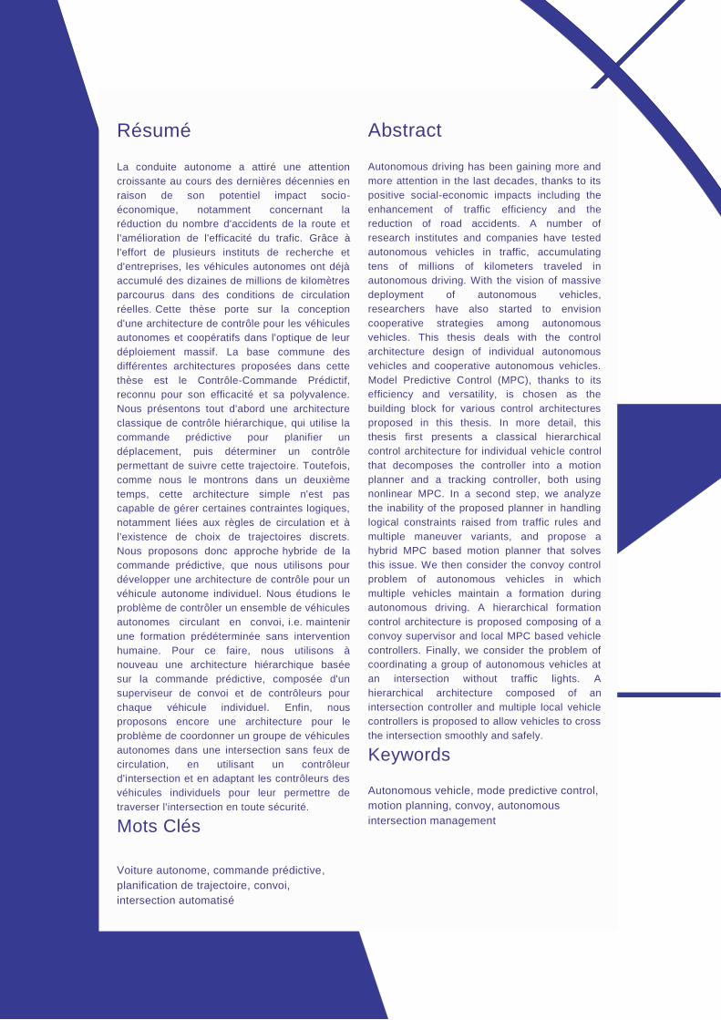
Résumé
La conduite autonome a attiré une attention
croissante au cours des dernières décennies en
raison de son potentiel impact socio-
économique, notamment concernant la
réduction du nombre d'accidents de la route et
l'amélioration de l'efficacité du trafic. Grâce à
l'effort de plusieurs instituts de recherche et
d'entreprises, les véhicules autonomes ont déjà
accumulé des dizaines de millions de kilomètres
parcourus dans des conditions de circulation
réelles. Cette thèse porte sur la conception
d'une architecture de contrôle pour les véhicules
autonomes et coopératifs dans l'optique de leur
déploiement massif. La base commune des
différentes architectures proposées dans cette
thèse est le Contrôle-Commande Prédictif,
reconnu pour son efficacité et sa polyvalence.
Nous présentons tout d'abord une architecture
classique de contrôle hiérarchique, qui utilise la
commande prédictive pour planifier un
déplacement, puis déterminer un contrôle
permettant de suivre cette trajectoire. Toutefois,
comme nous le montrons dans un deuxième
temps, cette architecture simple n'est pas
capable de gérer certaines contraintes logiques,
notamment liées aux règles de circulation et à
l'existence de choix de trajectoires discrets.
Nous proposons donc approche hybride de la
commande prédictive, que nous utilisons pour
développer une architecture de contrôle pour un
véhicule autonome individuel. Nous étudions le
problème de contrôler un ensemble de véhicules
autonomes circulant en convoi, i.e. maintenir
une formation prédéterminée sans intervention
humaine. Pour ce faire, nous utilisons à
nouveau une architecture hiérarchique basée
sur la commande prédictive, composée d'un
superviseur de convoi et de contrôleurs pour
chaque véhicule individuel. Enfin, nous
proposons encore une architecture pour le
problème de coordonner un groupe de véhicules
autonomes dans une intersection sans feux de
circulation, en utilisant un contrôleur
d'intersection et en adaptant les contrôleurs des
véhicules individuels pour leur permettre de
traverser l'intersection en toute sécurité.
Mots Clés
Voiture autonome, commande prédictive,
planification de trajectoire, convoi,
intersection automatisé
Abstract
Autonomous driving has been gaining more and
more attention in the last decades, thanks to its
positive social-economic impacts including the
enhancement of traffic efficiency and the
reduction of road accidents. A number of
research institutes and companies have tested
autonomous vehicles in traffic, accumulating
tens of millions of kilometers traveled in
autonomous driving. With the vision of massive
deployment of autonomous vehicles,
researchers have also started to envision
cooperative strategies among autonomous
vehicles. This thesis deals with the control
architecture design of individual autonomous
vehicles and cooperative autonomous vehicles.
Model Predictive Control (MPC), thanks to its
efficiency and versatility, is chosen as the
building block for various control architectures
proposed in this thesis. In more detail, this
thesis first presents a classical hierarchical
control architecture for individual vehicle control
that decomposes the controller into a motion
planner and a tracking controller, both using
nonlinear MPC. In a second step, we analyze
the inability of the proposed planner in handling
logical constraints raised from traffic rules and
multiple maneuver variants, and propose a
hybrid MPC based motion planner that solves
this issue. We then consider the convoy control
problem of autonomous vehicles in which
multiple vehicles maintain a formation during
autonomous driving. A hierarchical formation
control architecture is proposed composing of a
convoy supervisor and local MPC based vehicle
controllers. Finally, we consider the problem of
coordinating a group of autonomous vehicles at
an intersection without traffic lights. A
hierarchical architecture composed of an
intersection controller and multiple local vehicle
controllers is proposed to allow vehicles to cross
the intersection smoothly and safely.
Keywords
Autonomous vehicle, mode predictive control,
motion planning, convoy, autonomous
intersection management
