convex optimization - chapter 1-2 - university of …jliu/readinggroup/cvx-ch1-ch2.pdfconvex...
TRANSCRIPT

Convex Optimization - Chapter 1-2
Xiangru Lian
August 28, 2015
1

Mathematical optimization
minimize f0(x)
s.t. fj(x)6 0, j=1, ,m, (1)
x∈S
x. (x1, , xn). optimization variable.
f0. Rn→R. objective function.
fj. Rn→R, i=1, ,m. constraint functions.1
x∗. optimal or solution of the problem 1.
1. The constraint can be various and is not limited to 60.
2

S. basic feasible set.
Q. {x∈S |fj(x)6 0, j=1, ,m}. feasible set.
In general optimization problems are unsolvable.
3

Classification of optimization problems
1. Constrained problem.
2. Unconstrained problem.
3. Smooth problem.
4. Nonsmooth problem.
5. Linearly constrained problem.
a. Linear optimization problem.
b. Quadratic optimization problem.
6. Quadratically optimization problem.
7. Feasible. Strictly feasible......
They are just constrains on the type of f0, fj, S and x∗!
4

Classification of solutions
1. Global solution.
2. Local solution.
5

Analyze a method M
M. numerical method
P. a class of problems
Σ. Model . A known “part” of problem P .
O. Oracle. A unit answers the successive question of the method.
To solve the problem means to find an approximate solution toM with an accuracy ε> 0. Thus we need
Tε. a stopping criterion
Thus our problem class is
F ≡ (Σ,O, Tε).
6

Performance: The total amount of computational efforts requiredby M to solve P .
1. analytical complexity
2. arithmetical complexity
Optimal. if upper complexity bounds of the method are propor-tional to the lower complexity bound of the problem class
7

Example: Complexity bounds for globaloptimization
Consider a constrained minimization problem without functionalconstraints,
minx∈Bn
f(x). (2)
The basic feasible set of this problem is Bn, which is an n-dimen-sional box in Rn:
Bn={
x∈Rn|06x(i)6 1, i=1, , n}
. (3)
The distance is measured using l∞-norm.
8

We further assume that the function is L-Lipschitzian.
We can construct an optimal method for this problem and showthat it is not solvable by computers.
9

Main fields
• Goals of the methods
• Classes of functional components
◦ General global optimization: Let’s wait for quantum com-puters!
◦ Nonlinear optimization: We can find a local minimum underrestrictions[1].
◦ Convex optimization: We can find the global minimumunder restrictions.
◦ Interior-point polynomial-time methods: We can find theglobal minimum under restrictions for convex sets and func-tions with explicit structure.
10

• Description of the oracle
Convex optimization also benefits nonconvex optimization.
11

Convex sets
Line. Points of the form y= θ x1+ (1− θ) x2, where θ ∈R, formthe line passing through x1 and x2.
Line segment. y=x2+ θ (x1−x2) where 06 θ6 1.
Affine set. A set C ⊆ Rn is affine if the line through any two
distinct points in C lies in C.
Affine combination. θ1 x1+ + θk xk where θ1+ + θk = 1 isan affine combination of the points x1, , xk.
Theorem 1. If C is an affine set, x1, , xk ∈ C, then the affinecombination of x1, , xk also belongs to C.
12
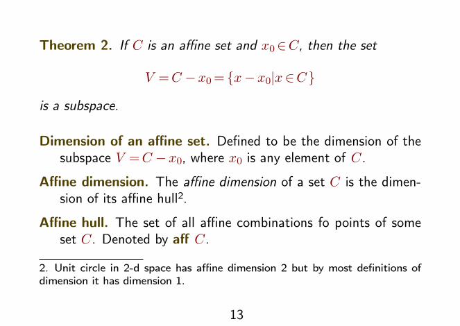
Theorem 2. If C is an affine set and x0∈C, then the set
V =C −x0= {x−x0|x∈C}
is a subspace.
Dimension of an affine set. Defined to be the dimension of thesubspace V =C −x0, where x0 is any element of C.
Affine dimension. The affine dimension of a set C is the dimen-sion of its affine hull2.
Affine hull. The set of all affine combinations fo points of someset C. Denoted by aff C.
2. Unit circle in 2-d space has affine dimension 2 but by most definitions of
dimension it has dimension 1.
13

Relative interior. The relative interior of the set C is the interiorrelative to aff C:
relintC = {x∈C |B(x, r)∩ aff C ⊆C for some r > 0}.
Relative boundary. The relative boundary of a set C isclC\relintC, where clC is the clojure of C.
The affine hull of C is the smallest affine set that contains C.
Convex set. A set C is convex if the line segment between anytwo points in C lies in C.
Convex combination. A convex combination of the points x1, ,
xk is θ1 x1 + � + θk xk, where θ1 + � + θk = 1 and θi > 0,i=1, , k.
14

Theorem 3. A set is convex iff it contains every convex combina-tion of its points.
Convex hull. A convex hull of a set C, denoted conv C, is theset of all convex combinations of points in C. It is the smallestconvex set that contains C.
Theorem 4. Suppose C ⊆Rn is convex and x is a random vectorwith x∈C with probability one. Then Ex∈C.
Cone. A set C is called a cone, or nonnegative homogeneous, iffor every x∈C and θ> 0 we have θ x∈C.
15

Convex cone. A set C is a convex cone if it is convex and a cone,which means for any x1, x2∈C and θ1, θ2> 0, we have
θ1x1+ θ2 x2∈C.
Conic combination. or nonnegative linear combination. A pointof the form θ1 x1+� + θkxk with θ1, , θk> 0.
Theorem 5. A set C is a convex cone iff it contains all coniccombinations of its elements.
Conic hull. A set of all conic combinations of points in C. This isthe smallest convex cone that contains C.
16

Examples
Hyperplane. A set of the form {x|aTx= b}, where a∈Rn, a� 0
and b∈R. (Normal vector is a.)
Halfspaces. A hyperplane divides Rn into two halfspaces. A
(closed) halfspace is a set of the form
{x|aTx6 b},
where a� 0. The open halfspace uses a strict inequality.
Euclidean ball. B(xc, r)= {x|‖x− xc‖26 r}= {xc+ r u|‖u‖261}.
17

Ellipsoid. E = {x|(x−xc)TP−1 (x−xc)6 1}= {xc+Au|‖u‖26
1}, where P =PT ≻ 0 and A is square and nonsingular.
Norm ball. {x|‖x−xc‖6 r}.
Theorem 6. Norm balls are convex.
Norm cone. {(x, t)|‖x‖6 t}⊆Rn+13.
3. For Euclidean norm:
{(x, t)∈Rn+1|‖x‖26 t}=
{(
x
t
)∣
∣
∣
∣
(
x
t
)
T(
I
−I
)(
x
t
)
6 0, t> 0
}
.
18

Figure 1. An example of norm cone.
This is also called Lorentz cone .
19

Polyhedron. The solution set of a finite number of linear equalitiesand inequalities and thus the intersection of a finite number ofhalf spaces and hyperplanes.
P = {x|ajT x 6 bj , j = 1, , m, cj
T x = dj , j = 1, ,
p}= {x|Ax4 b, C x= d}.
Theorem 7. The intersection of convex sets is a convex set.
Theorem 8. Polyhedra are convex sets.
Nonnegative orthant. The set of points with nonnegative com-ponents, i.e.,
R+n = {x∈R
n|xi> 0, i=1, , n}.
20

Affinely independent. k+1 points v0, , vk are affinely indepen-dent if v1− v0, , vk− v0 are linearly independent.
Simplexes. The simplex determined by k+1 affinely independentpoints v0, , vk∈Rn is
C = conv {v0, , vk}= {θ0 v0+� + θk vk|θ< 0, 1T θ=1}.
The affine dimension of this simplex is k.
Probability simplex. x< 0, 1Tx=1.
Unit simplex. x< 0,1Tx6 1.
The above simplex can be discribed using polyhedron.
21
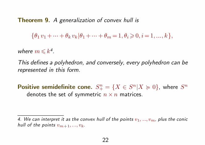
Theorem 9. A generalization of convex hull is
{θ1 v1+� + θk vk|θ1+� + θm=1, θi> 0, i=1, , k},
where m6 k4.
This defines a polyhedron, and conversely, every polyhedron can berepresented in this form.
Positive semidefinite cone. S+n = {X ∈ Sn|X < 0}, where Sn
denotes the set of symmetric n×n matrices.
4. We can interpret it as the convex hull of the points v1, , vm, plus the conichull of the points vm+1, , vk.
22

Operations that preserve convexity
Theorem 10. Convexity is preserved under intersection.
Theorem 11. Every closed convex set S is a (usually infinite)intersection of halfspaces. In fact, a closed convex set S is theintersection of all halfspaces that contain it:
S=⋂
{H|H halfspace, S ⊆H}.
Affine function. A function f :Rn→Rm is affine if it is a sum of
a linear function and a constant, i.e., f(x)=Ax+ b.
Theorem 12. Convexity is preserved under affine function, i.e., ifS is convex and f is an affine function, then f(S) is convex.
23

Note that the inverse function of an affine function is an affine func-tion. Examples of affine function include translation and projection.
Corollary 13. The partial sum of two convex sets S1,S2∈Rn×R
m
defined as
S= {(x, y1+ y2)|(x, y1)∈S1, (x, y2)∈S2},
where x∈Rn and yi∈R
m is convex.
Perspective function. P : Rn+1 → Rn, with domain dom P =
Rn ×R++, as P (z, t) = z/t. The perspective function scales
or normalizes vectors so the last component is one, and thendrops the last component.
24

Theorem 14. If C ⊆domP is convex, then its image
P (C)= {P (x)|x∈C}
is convex, where P is perspective function.
Proof. For any two points (x, z1), (y, z2) in C we have
θ x+(1− θ) y
θ z1+(1− θ) z2∈P (C).
From this we know the perspective function maps line segments toline segments and thus it preserves the convexity of sets. �
25

Theorem 15. The inverse image of a convex set under the per-spective function is also convex. If C ⊆R
n is convex, then
P−1(C)= {(x, t)∈Rn+1|x/t∈C, t> 0}
is convex.
Linear-fractional function. Compose the perspective functionwith an affine function. Suppose g: R
n → Rm+1 is affine:
g(x)=(
A
cT
)
x+(
b
d
)
, then
f =P ◦ g=(Ax+ b)/(cTx+ d), dom f = {x|cTx+ d> 0}
is a linear-fractional function. Affine function is a special caseof linear-fractional function.
26
Corollary 16. Linear-fractional functions preserve convexity.
Example 17. (Conditional probabilities) Let pij denoteprob(u = 1, v = j). Then the conditional probability f∗,j =
prob(u = ∗|v = j) =p∗,j
∑
k=1
n pkjis obtained by a linear-fractional
mapping from p∗,j. It follows that if C is a convex set of jointprobabilities for (u, v), then the associated set of conditional prob-abilities of u given v is also convex.
27

Generalized inequalities
Proper cone. A cone ⊆Rn that
1. convex
2. closed
3. solid, which means it has nonempty interior
4. pointed, which means that it is oriented, x∈K,−x∈K�
x=0.
proper cone can be used to define a partial ordering on Rn.
Generalized inequality. x 4K y� y − x ∈ K, x ≺K y�
y−x∈ intK.
28

Linear ordering. Any two points are comparable. 6 on R is linearordering but generalized inequality generally does not have thisproperty5.
Example 18. When K =R+, 4K is the usual ordering 6 on R.
Properties of generalized inequalities
1. Preserved under addition.
2. Transitive.
3. Preserved under nonnegative scaling.
4. Reflexive.
5. Antisymmetric.
5. This makes concepts like minimun and maximum more complicated.
29

6. Preserved under limits.
Minimum and minimal elements
Minimum. x∈S is the minimum element of S with respect to thegeneralized inequality 4K if for every y ∈S we have x4K y.
Minimal. x ∈ S is a minimal element of S with respect to thegeneralized inequality 4K if y ∈S, y4Kx only if y=x.
Maximum/Maximal. Defined in a similar way.
Theorem 19. If a set has a minimum element, then it is unique.A set can have many different minimal elements.
Theorem 20. A point x ∈ S is the minimum element of S iffS ⊆x+K.
30

Theorem 21. A point x∈S is a minimal element iff (x−K)∩S={x}.
Figure 2. Left: minimum. Right: minimal.
31

Example 22. (Minimum and minimal elements of a set ofsymmetric matrices) We associate with each A∈S++
n an ellipsoid
centered at the origin, given by EA= {x|xTA−1 x6 1}. We haveA4B iff EA⊆EB.
Let v1, , vk∈Rn be given and define
S= {P ∈S++n |vi
TP−1 vi6 1, i=1, , k},
which corresponds to the set of ellipsoids that contain the pointsv1, , vk. The set does not have a minimum element but haveminimal elements.
32

Figure 3. E2 is a minimal element.
33

Separating and supporting hyperplanes
Theorem 23. (Separating hyperplane theorem) Suppose C andD are two convex sets that do not intersect, i.e., C ∩D= ∅. Thenthere exists a� 0 and b such that aT x6 b for all x∈C and aT x> b
for all x ∈D. The hyperplane {x|aT x= b} is called a separatinghyperplane for the sets C and D.
Proof. Construct a plane orthogonal to the line formed by twopoints achieving the dist(C,D). �
Strict separation. If the inequalities in separation become strict,it is called a strict separation. Strict separation is not always
34

possible even for closed convex sets.
Theorem 24. Any two convex sets C and D, at least one of whichopen, are disjoint iff there exists a separating hyperplane.
Supporting hyperplane. Suppose C ⊆ Rn, and x0 is a point in
its boundary bdC = clC\intC. If a� 0 satisfies aT x6 aTx0
for all x ∈C, then the hyperplane {x|aT x= aT x0} is called asupporting hyperplane to C at the point x0
6.
6. This is equivalent to saying that the point x0 and the set C are separated
by the hyperplane.
35
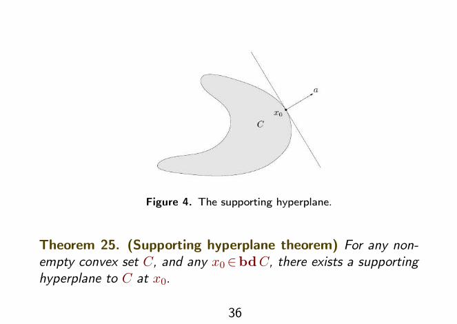
Figure 4. The supporting hyperplane.
Theorem 25. (Supporting hyperplane theorem) For any non-empty convex set C, and any x0∈bdC, there exists a supportinghyperplane to C at x0.
36

Theorem 26. If a set is closed, has nonempty interior, and hasa supporting hyperplane at every point in its boundary, then it isconvex.
37

Dual cones and generalized inequalities
Dual cone. Let K be a cone. The set K∗= {y |xT y> 0 for allx∈K} is called the dual cone of K.
Figure 5. y is in K∗ and z is not. Geometrically, y ∈K∗ iff y is
the normal of a hyperplane that supports K at the origin.
38

Theorem 27. K∗ is a cone, and is always convex, even when theoriginal cone is not.
Example 28. (Positive semidefinite cone) The positive semi-definite cone S+
n is self-dual under the standard inner product
tr(XY )=∑
i,j=1n
XijYji=∑
i,j=1n
Xij Yij.
Dual norm. ‖u‖∗= sup {uTx|‖x‖6 1}.
Example 29. (Dual of a norm cone) The dual of the norm cone
K= {(x, t)∈Rn+1|‖x‖6 t} is the cone defined by the dual norm,
39
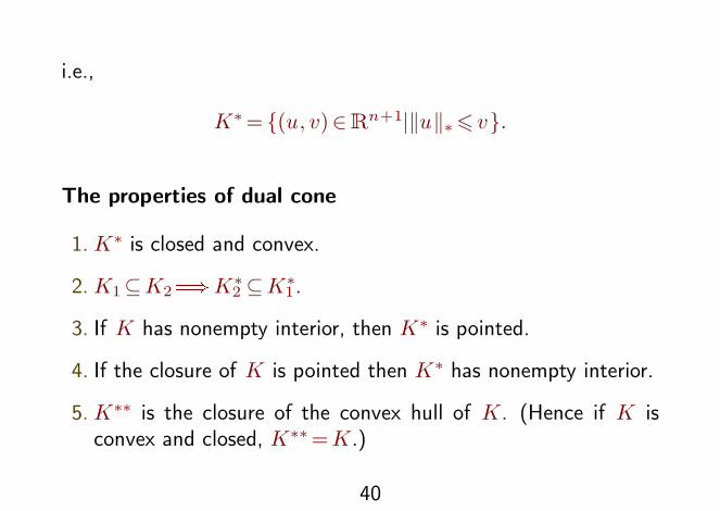
i.e.,
K∗= {(u, v)∈Rn+1|‖u‖∗6 v}.
The properties of dual cone
1. K∗ is closed and convex.
2. K1⊆K2� K2∗⊆K1
∗.
3. If K has nonempty interior, then K∗ is pointed.
4. If the closure of K is pointed then K∗ has nonempty interior.
5. K∗∗ is the closure of the convex hull of K. (Hence if K isconvex and closed, K∗∗=K.)
40
Theorem 30. If K is a proper cone, then so is its dual K∗.
Dual generalized inequalities
Dual generalized inequality. 4K∗. Note that if the convex coneK is proper, then K∗ is proper. Since for a proper cone K =K∗∗, the dual generalized inequality associated with 4K∗ is 4K.
Theorem 31.
1. x4K y iff λTx6λT y for all λ<K∗ 0.
2. x≺K y iff λTx<λT y for all λ<K∗ 0, λ� 0.
The geometric interpretation is easy to get.
41

Example 32. (Theorem of alternatives for linear strict gener-alized inequalities) Suppose K ⊆R
m is a proper cone. Considerthe strict generalized inequality
Ax≺K b,
where x∈Rn.
An alternative is there exists a λ such that
λTA=0, λT b6 0, λ<K∗ 0, λ� 0.
Theorem 33. x is the minimum element of S, with respect tothe generalized inequality 4K, iff for all λ ≻K∗ 0, x is the uniqueminimizer of λT z over z ∈S.
42

Figure 6. Dual characterization of minimum element. The point x
is the minimum element of the set S with respect to R+2 . This is
equivalent to: for every λ ≻ 0, the hyperplane {z |λT (z − x) = 0}
strictly supports S at x, i.e., contains S on one side, and touches it
only at x.
43

Theorem 34. If λ≻K∗ 0 and x minimizes λT z over z ∈S, then x
is minimal. Note that the converse is generally false.
Theorem 35. Provided that the set S is convex, we can say thatfor any minimal element x there exists a nonzero λ<K∗0 such thatx minimizes λT z over z ∈S.
44

45

Figure 8. Why the converse is not true and why < instead of ≻.
K =R+2 for example. Left. The point x1∈S1 is minimal, but is not a
minimizer of λT z over S1 for any λ≻ 0. Right. The point x2∈ S2 is
not minimal, but it does minimize λT z over z ∈S2 for λ=(0, 1)< 0.
46

Bibliography
[1] Xiangru Lian, Yijun Huang, Yuncheng Li and Ji Liu. Asynchronous
parallel stochastic gradient for nonconvex optimization. ArXiv preprint
arXiv:1506.08272 , , 2015.
47